Unsupervised Learning of Cell Activitiesin the Associative Cortex of BehavingMonkeys, Using Hidden Markov ModelsA thesis submitted in partial ful�llmentof the requirements for the degree ofMaster of SciencebyItay Gatsupervised byNaftali Tishby and Moshe AbelesInstitute of Computer Science andCenter for Neural ComputationThe Hebrew University of JerusalemJerusalem, Israel.January 1994

This thesis is dedicated to the memory of my beloved grandmother,Tova Kahana, who did not live to see its completion.

ii

AcknowledgmentsSpecial thanks are due to:� Dr. Naftali Tishby, my supervisor, who is in large measure re-sponsible for the completion of this study, for his ideas, continuinginterest and enthusiasm.� Prof. Moshe Abeles, who shared his knowledge unstintingly withme, for his important comments on the work in progress.� Dr. Hagai Bergman and Dr. Eilon Vaadia for sharing their datawith me, and for the numerous stimulating and encouraging dis-cussions of this work.� Yifat Prut, who gave of her time and helped me through thebiological background.� Iris Haalman and Hamutal Slovin for their valuable assistance inthe laboratory.� Yoram Singer, for his generous advice on mathematical and com-putational issues.� My wife, Tamar, who now knows more about behaving monkeysthan she ever thought possible, for her encouragement, support,and invaluable editing.This research was supported in part by a grant from the Unites StatesIsraeli Binational Science Foundation (BSF).iii

ContentsI Theoretical Background 11 Introduction 21.1 The Cell-Assembly hypothesis : : : : : : : : : : : : : : : : : : 21.2 Current analysis techniques of the cell assembly hypothesis : 31.2.1 Gravitational clustering : : : : : : : : : : : : : : : : : 41.2.2 JPST Histograms : : : : : : : : : : : : : : : : : : : : : 41.3 Models for simultaneous activity of several cells : : : : : : : : 51.3.1 Syn-Fire Chains : : : : : : : : : : : : : : : : : : : : : 51.3.2 Attractor Neural Network models : : : : : : : : : : : : 51.4 Statistical modeling : : : : : : : : : : : : : : : : : : : : : : : 61.5 Proposed model : : : : : : : : : : : : : : : : : : : : : : : : : : 71.5.1 Goals of the model : : : : : : : : : : : : : : : : : : : : 71.5.2 Elements of the model : : : : : : : : : : : : : : : : : : 71.5.3 Our working hypotheses : : : : : : : : : : : : : : : : : 82 Hidden Markov Models 92.1 Introduction : : : : : : : : : : : : : : : : : : : : : : : : : : : : 92.2 De�nitions : : : : : : : : : : : : : : : : : : : : : : : : : : : : : 92.3 Basic problems of the HMM : : : : : : : : : : : : : : : : : : : 122.4 Solution to the evaluation problem : : : : : : : : : : : : : : : 122.5 Solution to the decoding problem : : : : : : : : : : : : : : : : 132.6 Analysis of the learning problem : : : : : : : : : : : : : : : : 142.6.1 The Baum-Welch algorithm solution : : : : : : : : : : 152.6.2 The segmental K-means algorithm : : : : : : : : : : : 172.7 Clustering techniques used in HMM : : : : : : : : : : : : : : 172.7.1 KL-divergence : : : : : : : : : : : : : : : : : : : : : : 182.7.2 Characteristics of the KL divergence : : : : : : : : : : 212.8 Hidden Markov Model of multivariate Poisson probability ob-servation : : : : : : : : : : : : : : : : : : : : : : : : : : : : : : 222.8.1 Clustering data of multivariate Poisson probability : : 222.8.2 Maximum likelihood of multivariate Poisson process : 23II Model Implementation 25iv

3 Physiological Data and Preliminary Analysis 263.1 Frontal cortex as a source of data : : : : : : : : : : : : : : : : 263.2 Description of physiological experiment : : : : : : : : : : : : 273.2.1 Behavioral modes of the monkey : : : : : : : : : : : : 273.2.2 Data from recording session : : : : : : : : : : : : : : : 273.3 Basic tools of analysis : : : : : : : : : : : : : : : : : : : : : : 283.3.1 Dot display tool : : : : : : : : : : : : : : : : : : : : : 283.3.2 Temporal cross correlation tool : : : : : : : : : : : : : 293.4 Quality of cells recorded : : : : : : : : : : : : : : : : : : : : : 313.4.1 Isolation score given to cells during recording session : 313.4.2 Stationarity of a cell : : : : : : : : : : : : : : : : : : : 323.4.3 Firing rate of cells as a quality measure : : : : : : : : 333.4.4 Responsiveness of cells to events : : : : : : : : : : : : 344 Application of the Model 364.1 Data selection stage : : : : : : : : : : : : : : : : : : : : : : : 364.2 Computation of parameters used in the model : : : : : : : : : 374.3 Clustering of data vectors : : : : : : : : : : : : : : : : : : : : 384.4 Implementation of a full HMM : : : : : : : : : : : : : : : : : 394.5 Insertion of �ring rate cross-correlations into the model : : : 404.6 Search for correlation between state sequences and events : : 424.7 Display tools : : : : : : : : : : : : : : : : : : : : : : : : : : : 424.8 Temporal cross-correlation in di�erent states : : : : : : : : : 43III Results 445 Temporal Segmentation 455.1 Multi-cell activity in di�erent states : : : : : : : : : : : : : : 455.2 Consistency of clustering results : : : : : : : : : : : : : : : : 455.3 Coherency of the clustering results : : : : : : : : : : : : : : : 475.4 States' length distribution : : : : : : : : : : : : : : : : : : : : 495.5 E�ect of full HMM implementation : : : : : : : : : : : : : : : 515.5.1 Di�erences between the Baum-Welch algorithm andthe segmental K-means : : : : : : : : : : : : : : : : : 515.5.2 Changes in temporal segmentation due to a full HMM 525.6 E�ect of insertion of �ring rate cross-correlations into the model 535.7 Prediction of events based on state sequences : : : : : : : : : 546 Temporal Cross Correlations in di�erent states 596.1 Working hypotheses : : : : : : : : : : : : : : : : : : : : : : : 596.2 Cells with su�cient data : : : : : : : : : : : : : : : : : : : : : 596.3 Flat correlograms vs. functional connectivity : : : : : : : : : 636.4 Types of functional connectivity : : : : : : : : : : : : : : : : 66v

6.5 Modi�cation of pair-wise cross-correlation functions betweenstates : : : : : : : : : : : : : : : : : : : : : : : : : : : : : : : 676.6 Contamination of spike train as a cause of MPCS : : : : : : : 696.6.1 Insu�cient isolation between cells : : : : : : : : : : : 706.6.2 Cells recorded from the same electrode : : : : : : : : : 706.7 Types of MPCS : : : : : : : : : : : : : : : : : : : : : : : : : : 716.8 Changes in �ring rates of MPCS : : : : : : : : : : : : : : : : 74IV Discussion 777 Discussion 787.1 Hypotheses of the research : : : : : : : : : : : : : : : : : : : : 787.2 Interpretation of results : : : : : : : : : : : : : : : : : : : : : 787.2.1 Consistency of the model : : : : : : : : : : : : : : : : 787.2.2 Multi-dimensionality of the model : : : : : : : : : : : 797.2.3 Di�erences between behavioral modes : : : : : : : : : 797.2.4 Di�erent models used in the research : : : : : : : : : : 807.2.5 Prediction of events by the model : : : : : : : : : : : : 817.2.6 Changes in functional connectivity between states : : 817.3 Limitations of the model : : : : : : : : : : : : : : : : : : : : : 827.4 Conclusions and suggested further work : : : : : : : : : : : : 83

vi

List of Figures2.1 A simple Hidden Markov Model with 3 states. : : : : : : : : 103.1 A block diagram of the behavioral modes of the monkey. : : 283.2 An example of a dot-display. : : : : : : : : : : : : : : : : : : 303.3 An example of a cross-correlation function (correlogram) oftwo cells. : : : : : : : : : : : : : : : : : : : : : : : : : : : : : 313.4 An example of nonstationarity in the �ring rate of a cell, inwhich three distinct sections (marked in the left side of thedot-display) can be seen. : : : : : : : : : : : : : : : : : : : : 333.5 An example of di�erent �ring rates of two cells from the samerecording session. : : : : : : : : : : : : : : : : : : : : : : : : 343.6 An example of two cells that show di�erent responses to thesame stimulus. : : : : : : : : : : : : : : : : : : : : : : : : : : 354.1 An example of 8 spike trains of simultaneously recorded cells,with a short time �ring rate. : : : : : : : : : : : : : : : : : : 384.2 An example of execution of a K-means algorithm for di�erentnumber of states, using the same data. : : : : : : : : : : : : : 404.3 An example of execution of a K-means algorithm for two setsof data vectors. : : : : : : : : : : : : : : : : : : : : : : : : : : 415.1 The centroids of all the states. Each line represents the cen-troid of one state, and each bar on the line represents the�ring rate of one cell in that centroid. : : : : : : : : : : : : : 465.2 An example of three sets of clustering results. The upper setsare from the same behavioral mode, the lower set is from adi�erent behavioral mode. : : : : : : : : : : : : : : : : : : : : 475.3 An example of the coherency measure di�erence between twobehavioral modes, in di�erent starting conditions. : : : : : : : 495.4 An example of length distribution among segmentation of dif-ferent behavioral mode. : : : : : : : : : : : : : : : : : : : : : 505.5 An example of a typical segmentation of spike trains of 8 cells. 515.6 An example of two temporal segmentations of the same data(a.) and all their clusters' respective probabilities (b.) . : : : 565.7 An example of covariance matrices of 7 cells in 3 di�erent states. 57vii

5.8 An example of two segmentations and two labelings of spiketrains at di�erent time points of the same recording session. : 586.1 Two cross correlograms that show the e�ects of insu�cientdata. : : : : : : : : : : : : : : : : : : : : : : : : : : : : : : : : 606.2 An example of a cross-correlogram without su�cient data butwith clear functional connectivity : : : : : : : : : : : : : : : 626.3 An example of three correlograms. a: at correlation func-tion, b: nonzero correlation, c: questionable nonzero correlation 636.4 An example of a correlogram which is basically at althoughthe cross-correlation function crosses the signi�cance lines. : : 646.5 An example of di�erent types of functional connectivity : : : 676.6 All the correlograms of a pair of cells in di�erent states. : : : 686.7 An example of 6 correlograms showing di�erent functionalconnectivities. : : : : : : : : : : : : : : : : : : : : : : : : : : : 726.8 An example of wide to narrow functional connectivities. : : : 736.9 An example of inhibitory to at functional connectivities. : : 736.10 An example of narrow to at functional connectivity. : : : : : 746.11 An example of one sided to double sided functional connec-tivities. : : : : : : : : : : : : : : : : : : : : : : : : : : : : : : 766.12 An example of a dramatic change in �ring rate without anychange in the functional connectivity. : : : : : : : : : : : : : : 767.1 An example of HMM combined from simple task speci�c mod-els, and the embedding left-to-right model. : : : : : : : : : : 85

viii

List of Tables2.1 Simulated execution of the HMM shown in �gure 2.1 : : : : 114.1 Presentation of the recording sessions used throughout theexperiments. For each recording session, the number of well-isolated cells used is indicated, as is the total length of thesession (in seconds) and the cortical area from which the datawere recorded. These time tables are presented separately forthe \Go" mode and the \No-Go" mode. : : : : : : : : : : : : 375.1 The coherency of the best model for the \Go" mode and the\No-Go" mode at each of the recording sessions. : : : : : : : 485.2 The percentage of segments with lengths up to 1500 ms, forboth behavioral modes in all the recording sessions. : : : : : : 525.3 The likelihood values achieved in the di�erent training algo-rithms. : : : : : : : : : : : : : : : : : : : : : : : : : : : : : : : 525.4 Typical examples of prediction of events using states' sequences. 546.1 The percentage of data used for the temporal cross-correlation,from the total length of recorded data. : : : : : : : : : : : : : 606.2 The number of su�cient data cross-correlograms, among thecross-correlograms of the chosen cells. : : : : : : : : : : : : : 626.3 The number of non- at correlograms among the su�cientdata correlogram : : : : : : : : : : : : : : : : : : : : : : : : : 656.4 The classi�cation of non- at correlograms into four types offunctional connectivity : : : : : : : : : : : : : : : : : : : : : : 666.5 The number of MPCS occurrences - classi�ed into \Go" trialsand \No-Go" trials, and compared with the total number ofsu�cient data cell-pairs. : : : : : : : : : : : : : : : : : : : : : 696.6 Classi�cation of MPCS occurrences for each recording sessioninto three groups: A or B types, B or C types, and all theother types. : : : : : : : : : : : : : : : : : : : : : : : : : : : : 706.7 The number of MPCS occurrences from the same electrodeand from di�erent electrodes, in the 2 behavioral modes. : : : 716.8 Comparison between changes in �ring rate vs. changes inMPCS. : : : : : : : : : : : : : : : : : : : : : : : : : : : : : : : 75ix

AbstractHebb hypothesized in 1949 that the basic information processing unit in the cortex is a cell-assembly which can act, brie y, as a closed system after stimulation has ceased, and constitutesthe simplest instance of a representative process. This hypothesized cell-assembly may includethousands of cells in a highly interconnected network. The cell-assembly hypothesis shifts the focusfrom the single cell to the complete network activity. So far, there has been no general methodfor relating extracellular electrophysiological measured activity of neurons in the associative cortexto the underlying network or the cell-assembly states. It is proposed here to model such data asa pair-wise correlated multivariate Poisson process. Based on these parameters, a Hidden MarkovModel was computed. This modeling yielded a temporal segmentation and labeling of the datainto a sequence of states.The �rst hypothesis of this work was that a connection exists between the states of the model andthe behavioral events of the animal. i.e. based on the sequence of states of the model, the observedactions of the animal could be predicted. The second hypothesis was that a connection existsbetween the states de�ned above and the functional interaction between cells, i.e. the functionalinteraction between pairs of cells changes in di�erent cognitive states.The application of this approach was demonstrated for temporal segmentation of the �ringpatterns, and for characterization of the cortical responses to external stimuli. This modeling wasapplied to 6 recording sessions of several single-unit recordings from behaving monkeys. At eachsession, 6-8 single-unit spike trains were recorded simultaneously. Using the Hidden Markov Model,two behavioral modes of the monkey were signi�cantly discriminated. The two behavioral modeswere characterized by di�erent �ring patterns, as well as by the level of coherency of their multi-unit �ring activity. The result of the modeling showed a high degree of consistency, which impliesthat the model succeeds in capturing a basic structure underlying the data. Signi�cant changeswere found in the temporal cross-correlation of the same pair of cells in di�erent states, indicatingdi�erent functional connectivities of the small network being recorded. These changes suggest thatthe modeling captures the activity of the network and that the states of the model can be relatedto the cognitive states of the cortex.

Part ITheoretical Background

1

Chapter 1Introduction1.1 The Cell-Assembly hypothesisThe cortex is considered the part of the human brain that is essential to the processing of informa-tion. The human cortex consists of a vast number of neurons (around 1010), which are connectedvia synapses, each neuron typically receiving 104 - 105 synapses [1]. It is assumed that this structureenables the brain to perform the complicated actions it is capable of. The basic question emergingfrom this structure concerns its relationship to the complex action for which it is responsible.One of the common hypotheses related to this question is the Cell-Assembly Hypothesis sug-gested by Hebb in 1949. \It is proposed �rst that a repeated stimulation of speci�c receptors will leadslowly to the formation of an \assembly" of association-area cells, which can act brie y as a closedsystem after stimulation has ceased; this prolongs the time during which the structural changes oflearning can occur and constitutes the simplest instance of a representative process (image or idea)"[36] This hypothesized cell-assembly may include thousands of cells in a highly interconnected net-work. The cell-assembly is further characterized by stronger than average connections between thecells which comprise it. The organization of the cell-assembly is achieved via these strong con-nections, i.e. there is a mechanism that creates these assemblies by strengthening the connectionbetween cells. Hebb further hypothesized that this mechanism is related to the ordered activa-tion of cells, that is, whenever two cells are activated one after the other, the connection betweenthem is reinforced. The cell-assembly is a group of interconnected cells, whose participation in thecell-assembly is not determined by proximity. One cell may participate in several cell-assemblies,and it is possible for cells which are next to each other not to be part of the same cell-assembly.The de�nition of a cell-assembly is, therefore, more of a functional than an anatomical one, asthe cell-assembly is not de�ned by speci�c physiological locations. The information processing inthe cortex is dynamic in time, and tends to alternate between di�erent activation states of onecell-assembly, and between activations of several cell-assemblies. The same cell-assembly may beutilized in di�erent computational tasks. Thus, a typical computation process consists of a se-quence of these functional units (cell-assemblies), and will henceforth be referred to as a sequenceof cognitive states.De�ning the cell-assembly as the basic unit of processing suggests the notion of the statisticalbehavior of a single cell in that network: \in a larger system a statistical constancy might be quitepredictable" [36]. This statistical behavior is also expected due to the fact that a single cell may2

CHAPTER 1. INTRODUCTION 3participate in a number of assemblies. The notion of the cell-assembly has been formalized sinceHebb �rst suggested it [72, 54]. Furthermore, the cell-assembly hypothesis matches the up-to-dateknowledge about the anatomical structure of the cortex, especially the structure of high corticalareas - the associative cortex [31].1.2 Current analysis techniques of the cell assembly hypothesisOne of the traditional views of the neuronal activity stressed the importance of the activity ofsingle cells [13]. Methods based on this view show quite remarkable results in many cortical andsub-cortical areas. These results include relationships between highly speci�c changes of �ringrates and sensory or motor processing, or even cognitive and other higher brain function such asperceptual analysis of sensory input, selective attention, short time memory, etc. [23, 53, 35]. Theusual way of computing the activity of a single cell is by the peri-stimulus-time (PST) histogram,which is an average measure of the �ring rate probability relative to the stimulus presented. In highcortical areas it was found that in order to attain a reasonably smoothed PST it was necessary toaverage the activity over many repeated activations (typically at least 30 to 50). This fact by itselfshows that the requisite information cannot be coded in the activity of a single cell alone [65]. Still,the PST histogram is a valuable tool for measuring the �ring rate of cells, and can give a exibleestimation in the time domain.The cell-assembly hypothesis shifts the focus from the single neuron to the complete networkactivity. This view has led several laboratories to develop technology for simultaneous multi-cellularrecording from a small region in the associative cortex [1, 43, 44]. Extracellular electrophysiologicalmeasurements have so far obtained simultaneous recordings from just a few randomly selectedneurons (about 10) in the cortex, a negligible number compared to the size of the hypothesizedcell-assembly. These are recordings of the simultaneous �ring activities of the randomly selectedneurons of a behaving animal. Behaving animal is the term used to describe a conscious animalengaged in a speci�c, pre-de�ned activity. The discrete action potentials shall be called henceforththe spike trains of cells.In order to process this multi-cellular recording information, and to relate the data to thehypothesized cell-assembly, several techniques have been developed. The best known of theminvolves computing the pair-wise cross-correlation function between cells [57, 34, 55]. This techniqueanalyzes the spike trains of a pair of cells for possible temporal relations, by computing the cross-correlation function of the two spike trains. Departures from background in the correlogram aretaken as an indication of functional connectivity between the two cells [8, 69]. The term functionalconnectivity (also referred to as e�ective connectivity) [50, 57] is used in this context because ofthe cell-assembly hypothesis which implies that this correlation is due to the activity of the wholecell-assembly.This analysis method su�ers from some serious limitations:1. The number of cross-correlation functions grows quadratically with the number of recordedcells: for N cells one has N(N�1)=2 di�erent pairs. This number is further multiplied by thenumber of di�erent conditions under which these cells are checked (di�erent stimuli, di�erentbehavioral modes of the animal, etc.). This growth makes the method inapplicable even fora small number of cells.

CHAPTER 1. INTRODUCTION 42. The di�culty of monitoring the dynamics of cross-correlation over time.3. The di�culty of processing information from more than two or three cells simultaneously.4. The need for long stationary recordings that, presumably, originate from the same activationof the cell-assembly.The last point raises the issue of time in this analysis method. Not only does the cross-correlationanalysis require long time intervals of spike trains, it also necessitates the repetitive measurementsof these same intervals in order to reach signi�cant results. The use of repetitive measurementsrests on the assumption that under similar external circumstances, the recorded cells behave in asimilar way. This assumption ignores the following facts:� The recorded cells are randomly selected from a much larger network. As a result of this,and of the statistical nature of their behavior, single cells may function in di�erent ways atdi�erent points of time, while the whole network acts in a consistent manner.� The ability to produce exactly the same external circumstances in each repetition is verylimited.There are several methods that attempt to overcome some of these limitations. Most notableamong them are the Gravitational Clustering [32, 31], and the Joint Peri Stimulus Time Histogram(JPST)[7, 8].1.2.1 Gravitational clusteringGravitational clustering attempts to overcome the enormous proliferation of cross-correlation func-tions to be examined, and transform them into a single computation. This transformation is carriedout by modeling each of the N neurons as particles in an N space. All particles are initially equidis-tant. Each particle carries a charge which is incremented with every �ring of the correspondingcell, and then decays with an appropriate time constant. These particles attract each other with aforce proportional to the product of their charges. Thus they move towards each other with a ve-locity proportional to the degree of �ring correlation. This system converges into clusters of highlycorrelated cells (if such exist). The clustering process over time, and the clusters formed, tell usabout the nature of these correlations. This computation is particularly e�ective in screening largeamounts of data, and identifying the spike trains that should undergo a more detailed inspection.Considerably more detailed description of the gravity transformation can be found in [30, 7].The main problem of this method is the cross talk between cells. That is, a highly correlatedactivity of two cells alters the distance of these cells from the other cells. This change of distanceis not the result of correlated activity between these two cells and other cells. Another problem isthat this method is not sensitive to high order correlations between cells.1.2.2 JPST HistogramsThe Joint Peri Stimulus Time Histogram attempts to overcome the problem of dynamics foundin the cross-correlation between cells. This is done by drawing a scatter diagram of the co-�ringof two cells, time-locked to the occurrence of a certain event, and counting the number of joint

CHAPTER 1. INTRODUCTION 5occurrences in a cartesian grid of bins. The output of this process is a matrix of counts M , inwhich each element Mij is the average co-�ring of the two cells within a speci�c time interval (theith bin for the �rst cell and jth bin for the second cell), time-locked to the event used as a trigger.Further normalization is applied to this matrix on the basis of the expected amount of co-�ring(computed from each neuron PST). The normalized matrix provides evidence for the dynamics ofthe functional connectivity between the neurons, relative to the event used.This method is appropriate for studying the connection between two cells, but su�ers from thesame problems as the cross-correlation technique, regarding the large number of graphs and thetime needed to scan and process them.1.3 Models for simultaneous activity of several cellsSeveral models and hypotheses followed Hebb's ideas. Two of them are described here: the Syn-FireChain [3, 2, 6], and the Attractor Neural Network [37, 11]. These models assume that \learning" isbased on selective modi�cation of the connectivity among neurons, and \computations" are carriedout by selective activation of interconnected neurons. These models do not contradict each other,and can be viewed as di�erent aspects of the same physical system.1.3.1 Syn-Fire ChainsThe Syn-Fire Chain model is based on synchronous temporal structures of spike trains. Accordingto this model, the activity in the cortex is propagated in a network made of a chain of diverging-converging links, where each of these links is made of several neurons. The information in thismodel is propagated in the chain by secure transmission of a synchronous volley from link to link.This model, like the cell-assembly, takes not only an anatomical form, but also a functional one, i.e.the neurons participating in the Syn-Fire Chain may be scattered and intermingled with each otherand with many other neurons. Furthermore,the same neuron may participate in several syn-�rechains. This model predicts the existence of temporal structures in the spike trains of cells, andanalyzes them [3, 5].1.3.2 Attractor Neural Network modelsIn the last decade there has been impressive development in the �eld of physical models of neuron-like networks, many of which can be analyzed by statistical mechanics, via the analog with spin-glasssystems. One of the notable models is the Attractor Neural Network (ANN). This model presentsa network consisting of a large number of simple look-alike units, that imitate some of the basicfunctions of real neural networks. Each of these units is connected via weighted links to some, orall, of the other units, and alters its state according to these links and to its current state. Theseunits are, therefore, referred to as neurons, and the whole system is referred to as a neural network.This description de�nes a dynamical system, which for any given initial set of neuron states,goes on wandering among the 2N possible con�gurations of the network, where N is the numberof neurons. The basic concept in this framework is the attractor. An attractor is de�ned as astate (or a cycle of states) of the network that is reached through the dynamics of the system,from di�erent initial con�gurations. Reaching an attractor in the network can be interpreted asrecalling a pattern that is stored in memory. The attractors reached can be static ones (an example

CHAPTER 1. INTRODUCTION 6of this type can be seen in the Hope�eld model [37]). In a more general setup, cyclic attractorsmay appear.This description suggests that an ANN is capable of performing memory recall by using theattractors of the network [41]. This ability may be seen as the �rst step towards a computingnetwork that dynamically goes through a sequence of alternating attractors. This sequence ofattractors may be related to the ideas concerning the cell-assembly hypothesis mentioned above[42].1.4 Statistical modelingOne of the basic tools used in this work in order to combine the information about cell-assembliesand the recording from behaving animals, is the statistical modeling [22]. The basic task to becarried out on the data is to \model" it, i.e. to be able to capture the inherent structure ofinformation it contains. This "capturing" would allow the model to analyze the information in thedata, and to make predictions on the basis of what has been modeled.In the �eld of learning theory, a separation exists between algorithmic procedures that use la-beled samples for discrimination and are said to be supervised, and procedures that use unlabeledsamples and are called unsupervised. All the methods of analyzing the data collected from the cor-tex, described above, were processed in a supervised manner. The labeling used in these processeswas the timing of external events in the experiment.Unsupervised modeling has both bene�ts and disadvantages in the modeling of cortex activity,when compared to supervised modeling. The basic advantage of this method is that it enables thedirect modeling of the data without making assumptions as to the nature of the data. For example,the modeling techniques shown above assume a direct connection between events of the experiment(stimuli to the animal, or behavioral actions) and the sequence of cognitive states the cortex goesthrough. This assumption may not always hold, as explained before. An attempt to model thatdata in an unsupervised manner, on the other hand, may reveal a direct connection betweenthe spike trains of several cells and the cognitive states of the cortex. The clear disadvantage ofunsupervised learning is that only a collection of unclassi�ed examples exists - so the basic conceptsare not known in advance.In this work we will focus on one type of unsupervised learning procedure. This type assumesthat the data is unlabeled, but that the class of functions of the underlying probabilities producingthese samples is known. An example of this type is the classi�cation of samples received from amixture of two Gaussians with di�erent means and variances. The statistical modeling in this caseis required to �nd a way to estimate the parameters of the probability function. In the Gaussianmixture case, these are the means and variances of the processes.While this research was in progress, another work in the same �eld was begun in our laboratory[64]. In this work the same data was modeled using a HMM, but with two important di�erences:1. The model was built in a supervised manner, using only the spike trains of the �rst 4 secondsafter a pre-de�ned external stimulus.2. The observations of the model were computed every ms, and included the information asto which cell emitted a spike. The possibility that two or more cells emitted spikes wasdisregarded.

CHAPTER 1. INTRODUCTION 7This data used by the model was divided into four di�erent groups (according to the type ofstimulus presented to the animal), and after appropriate training the model was able to predictthe stimulus from the spike trains. While writing this report, another relevant work was broughtto our attention [63]. The recording in this work were taken from the visual cortex of anesthetizedmonkeys. In this work another supervised HMM analysis of spike trains was carried out. Theresults of this work show the possibility of predicting the di�erent visual stimuli presented to theanesthetized animal from the recorded spike trains.1.5 Proposed model1.5.1 Goals of the modelThe aim of the work presented here is to �nd a connection between the hypothesized cell-assembliesand the attractors introduced in ANN, and the spike trains of several cells recorded simultaneously.It is related to a core physiological question: whether the computations in the brain are carriedout by cell-assembly-like circuits, i.e. by transitions between distinct states. The time constants ofthese processes are assumed to be in the order of tens to hundreds of ms, and these are the timeconstants that will be used in the model.The model presented tries to overcome some of the problems of the current analysis techniquesdescribed above, in the following ways:� The relation between the states and the parameters of the model based on the spike trains isa direct one, i.e. those spike trains are the stochastic output of the computed states.� The estimation of the states is based on stochastic point-wise processes, i.e. repetitions ofintervals of the data are not averaged.� The computations do not make use of the events marked on the spike trains (such as thestimulus to the animal or the behavioral reactions).� The computation is based on a truly vectorial model which uses all the parameters computedfrom the spike trains simultaneously, i.e. computation is carried out in an N dimensionalspace, where N is the number of cells used.1.5.2 Elements of the modelThe analysis method presented in this work is based on a model with the following assumptions:� The spike trains are produced as a stochastic output from a Markov process.� The states of the Markov process change according to speci�c transition probabilities.� The states cannot be observed directly. Only the stochastic output of the state at each timeis observable.One type of such a process is the �rst order Hidden Markov Model (HMM) presented in Chapter2 in detail.

CHAPTER 1. INTRODUCTION 8In order to model the spike trains of cells with a HMM, the architecture of that model must bechosen, and its parameters estimated [29]. In this realization of the model, the simultaneous �ringrates of the cells, and the pair-wise cross-correlation between them, were used as the statisticalmeasure of the states. The �ring rates were modeled as a multivariate Poisson process. Based onthese estimated parameters, a Hidden Markov Model was computed. This modeling also yielded atemporal segmentation of the data into sequences of states.1.5.3 Our working hypothesesThe �rst hypothesis of the model is that a connection exists between the states of the model andthe behavioral events of the animal. This connection may be found in a correspondence of themodel to some speci�c neural activity. It may also be found in the ability to predict observedactions based on the sequence of states of the model. The states of the model estimated from thedata are assumed to be connected to a sequence of cognitive states related to the action taken bythe animal. The purpose of this work is to substantiate this relationship in a scienti�c qualitativemanner. In order to check this hypothesis, di�erent aspects of the temporal segmentation of thedata will be checked. These aspects include:� The examination of state representatives on the basis of their mutual activity.� The search for di�erences between behavioral modes.� The coherency of the model, i.e. how accurately does the model describe the data.� The ability of the model to predict events from the states (or sequences of states).The second hypothesis is that a connection exists between the states de�ned above and thefunctional connectivity between cells, i.e. the functional connectivity between pairs of cells changesin di�erent cognitive states. In order to check this hypothesis, the temporal cross-correlationfunctions between the same pair of cells will be computed for di�erent states of the model. Thesefunctions will be compared, and changes between states will be sought. If the model does indeedcaptures some notion of states' activity in the cortex, the cross-correlations are expected to showdi�erent types of functional connectivity in di�erent states.

Chapter 2Hidden Markov Models2.1 IntroductionHidden Markov Modeling (HMM) is a probabilistic technique for the study of time series [58, 19, 60].Hidden Markov theory permits modeling with many of the classical probability distributions. Thecosts of implementation are linear in the length of the data. These and other desirable features havemade Hidden Markov methods increasingly attractive for tackling problems in language, speech andsignal processing.Although initially introduced and studied in the late 1960s and early 1970s, Hidden MarkovModeling has become increasingly popular in the last several years. There are two strong reasonswhy this has occurred. First, the models are very rich in mathematical structure and hence canform the theoretical basis for use in a wide range of applications. Second, the models, when appliedproperly, work very well in practice for several important applications [46, 61].2.2 De�nitionsThe basic concepts of the Hidden Markov Models are as follows:Given a system which may be described at any time as being in one of a set of N distinctstates, S1,S2, � � � ,SN , as illustrated in �gure 2.1 (where N = 3 for simplicity). At regularly spaceddiscrete times, the system undergoes a change of state (possibly back to the same state) accordingto a set of probabilities associated with the state. These probabilities are denoted in the �gure bya(i; j) variables. The actual sequence of states would be denoted as qt 1 � t � T , where T isthe number of discrete steps the systems undergoes. A full probabilistic description of the abovesystem would, in general, require speci�cation of the current state (at time t) as well as all thepreceding states. For a special case of a �rst order Markov chain, this probabilistic description istruncated to just the current and predecessor state. Furthermore, the only considered processes arethe ones in which the probability is stationary, i.e. the probabilities ai;j are independent of time.In the example shown in �gure 2.1 all the transitions between states are allowed, i.e. are with anon-zero probability. This is a special case of Markov models in which ergodicity is kept. Thereexist also non-ergodic models in which some of the transition probabilities are not allowed (set tozero), thus producing a speci�c structure of states.The above stochastic process could be called an observable Markov chain since the output of9

CHAPTER 2. HIDDEN MARKOV MODELS 101 2S S

S3

a(3,2)

a(2,3)

a(3,3)

a(2,2)a(1,1)

a(3,1)

a(1,3)

a(1,2)

a(2,1)

b1 b3 b2

Figure 2.1: A simple Hidden Markov Model with 3 states.the process is a set of states at each instant of time, where each state corresponds to a physicalevent.In the Hidden Markov Models, the model described above is extended to include the case wherethe observation is a probabilistic function of the state. The resulting model is a double embeddedstochastic process with an underlying stochastic process that is not observable, but can only beobserved through another set of stochastic processes that produce the sequence of observations.These observations may be discrete symbols from a �nite alphabet, or continuous variables from aknown distribution.This double-embedded stochastic process is shown in �gure 2.1 in the following manner: thestates are shown to be hidden by the dotted horizontal line presented in the upper part of the�gure, where the observation of each state is shown as a dotted arrow emerging from the state andcrossing that horizontal line.The formal constituents of the discrete HMM are as follows:1. N , The number of states in the model.

CHAPTER 2. HIDDEN MARKOV MODELS 112. M , The number of distinct observation symbols per state, i.e., the discrete alphabet size.This description will be altered later to include the continuous distributions.3. A, The state transition probability distribution matrix.4. B, The observation symbol probability distribution matrix.5. �, The initial state distribution vector.Given appropriate values of N ,M ,A,B and �, the HMM can be used as a generator to give anobservation sequence O = O1O2O3 � � �OT ; (2:1)where each observation Ot is one of the symbols, and T is the number of observations in thesequence. The symbols are denoted as V = v1; v2 � � �vM in the discrete case. The execution of theHMM generator is as follows:1. Choose an initial state q1 = Si according to the initial state distribution �.2. Set t = 1.3. Choose Ot = vk according to the symbol probability distribution in state Si, i.e. bj(k).4. Transit to a new state qt+1 = Sj according to the state transition probability distribution forstate Si, i.e. aij .5. if t = T stop.6. t ! t + 17. Go to step 3.An example of this process may be seen in table 2.1. This example is related to the HiddenMarkov Model presented in �gure 2.1. In this example, the size of the alphabet is 4, thus 4 di�erentsymbols may be emitted from the states. The hidden states are presented in the top line and theobservations produced by them are presented in the bottom line.States q1 q1 q2 q2 q2 q2 q1 q3 q3 q1 q2 q2 q2 q3 q3Symbols v3 v3 v1 v2 v1 v1 v3 v4 v2 v1 v1 v1 v2 v2 v4Table 2.1: Simulated execution of the HMM shown in �gure 2.1The above procedure can be seen as both a generator of observations, and a model for how agiven observation sequence was generated by an appropriate HMM. A complete description of themodel could be given as � = (A;B; �) : (2:2)

CHAPTER 2. HIDDEN MARKOV MODELS 12The observations Ot of the Hidden Markov Model as shown till now were discrete symbols froma �nite alphabet v1; v2 � � � ; vM . For many problems, this assumption is not a straightforward one,and requires the quantization of continuous signals into discrete symbols. There exists, however,a very elegant modi�cation to the basic HMM that enables the insertion of continuous signalsdirectly into the model [61]. From this point on the symbols used in the model are continuous,from a known distribution. This distribution should obey some restrictions.The most general representation of such a probability density function is:bi(O) = MXm=1 cimP [O; �im;Ujm] ; (2:3)where bi is the probability of emitting an output vector (observation) O at state i, cim is themixture coe�cient for the mth mixture in state i and P is any log-concave or elliptically symmetricdensity, with mean vector �im and covariance matrix Uim for the mth mixture component in statei [39].2.3 Basic problems of the HMMUse of the HMM usually raises a few questions about the model [60].1. Given the observation sequence O = O1 O2 � � � OT , and a model � = (A,B,�), how do wee�ciently compute P (Oj�), i.e. the probability of the observation sequence, given the model? This problem is referred to as the evaluation problem.2. Given the observation sequence O = O1 O2 � � � OT , and a model � = (A,B,�), how do wechoose a corresponding state sequence Q = q1 q2 � � � qT which is optimal in some meaningfulsense (i.e., best \explains" the observations) ? This problem is referred to as the decodingproblem.3. How do we adjust the model parameters � = (A,B,�) to maximize P (Oj�) ? This problemis referred to as the learning problem, or the estimation problem.The solution of these problems is important for the realization of the model. When severalHidden Markovmodels exist and an observation sequence is presented, the solution to the evaluationproblem is used to determine the most probable model for describing the data. After �nding the bestmodel to �t the data, the solution to the decoding problem helps reveal the underlying structureof the problem, i.e. the hidden states of the model. The solution to the learning problem is usedto build the models used in the previous problems.2.4 Solution to the evaluation problemThe straightforward solution to that problem is:P (Oj�) = XallQP (OjQ;�)P (Qj�) = Xq1;q2;���;qT �q1bq1(O1)aq1q2bq2(O2) � � �aqT�1qT bqT (OT ) ; (2:4)

CHAPTER 2. HIDDEN MARKOV MODELS 13where q1; q2; � � � ; qT is the permutation of all state sequences of length T . The problem withthis approach is the number of calculations needed, which is in the order of TNT . This may beinfeasible even for small values of N and T .The Forward-Backward Procedure can be used to compute this problem much more e�ciently.In this algorithm a forward variable �t(i) de�ned as:�t(i) def= P (O1O2 � � �Ot; qt = Sij�) ; (2:5)is computed. This variable can be used throughout the following procedure:1. Initialization: �1(i) = �ibi(O1) 1 � i � N : (2:6)2. Induction: �t+1(j) = [ NXi=1 �t(i)aij]bj(Ot+1) 1 � t � T � 1; 1 < j < N : (2:7)3. Termination: P (Oj�) = NXi=1 �T (i) : (2:8)This procedure computes the required probability in its termination step and the calculation ofthis variable involves only an order of N2T operations. This number is quite feasible for implemen-tation. This procedure is a special case of dynamic programming [16, 66], which is a a mathematicalconcept used for the analysis of sequential decision problems, based on the principle of optimal-ity. \An optimal policy has the property that whatever the initial state and initial decision are,the remaining decisions must constitute an optimal policy with regard to the state resulting fromthe �rst decision \ [17]. The use of this technique assure the correctness and optimality of theforward-backward procedure.The computation of a backward variable can be carried out in a similar manner [60]. Thisvariable is de�ned as: �t(i) def= P (Ot+1Ot+2 � � �OT jqt = Si;�) : (2:9)Both forward and backward variables can be used to solve the �rst problem of the HMM.2.5 Solution to the decoding problemIn order to solve the decoding problem, the notion of optimality has to be de�ned more speci�cally.Optimality may be de�ned in several ways, among them:� The state sequence in which every state qt is individually most likely.� The state sequence that maximizes the expected number of correct pairs of states.� The state sequence that maximizes the expected number of correct triplets of states.

CHAPTER 2. HIDDEN MARKOV MODELS 14The most widely used criterion for optimality is to �nd the single best state sequence (path),i.e. to maximize P (QjO;�). The algorithm that solves this problem is called a Viterbi algorithmand it is a form of the previously described dynamic programming, for a stochastic system [71, 24].The Viterbi algorithm �nds the single best state sequence, Q = q1; q2 � � � ; qT , for the givenobservation sequence O = O1; O2; � � � ; OT , and uses the following quantity:�t(i) def= maxq1;q2;���;qt�1 P [q1q2 � � �qt = i; O1O2 � � �Otj�] ; (2:10)i.e., �t(i) is the best score (highest probability) along a single path, at time t, which accountsfor the �rst t observations and ends in state Si. By induction we have:�t+1(j) = [maxi �t(i)aij]bj(Ot+1) : (2:11)To actually retrieve the state sequence, the track of the argument which maximizes 2.11 mustbe kept. This is done via the auxiliary array t(j).The complete procedure is stated as follows:1. Initialization: �1(i) = �ibi(O1); 1 � i � N (2.12) 1(i) = 0 : (2.13)Recursion: �t(j) = max1�i�N [�t�1(i)aij]bj(Ot); 2 � t � T 1 � j � N : (2.14) t(j) = argmax1�i�N [�t�1(i)aij]; 2 � t � T 1 � j � N : (2.15)2. Termination: P � = max1�i�N [�T (i)] : (2:16)q�T = arg max1�i�N [�T (i)] : (2:17)3. Path (state sequence) backtracking:q�t = t+1(q�t+1); t = T � 1; T � 2; � � � ; 1 : (2:18)2.6 Analysis of the learning problemThis problem is involved in �nding the model � that maximizes P (Oj�) given a �xed O, i.e. thelikelihood function given the observation. This problem can be described, therefore, as �nding theglobal maximum of the likelihood function (ML). There is no known way to analytically computethe global maximum of the likelihood function. It is possible, however, to �nd local maxima of thisfunction, and two of these algorithms will be shown here. These algorithm are:1. The Baum-Welch method, also known as the EM (expectation modi�cation) method [21, 15,73, 14].

CHAPTER 2. HIDDEN MARKOV MODELS 152. The Segmental K-means technique [46, 40, 62].The Baum-Welch algorithm provides an estimate which locally maximizes the likelihood func-tion of the given observation sequence, and the segmental K-means algorithm provides an estimatewhich locally maximizes the joint likelihood of the observation sequence and the most likely statesequence.2.6.1 The Baum-Welch algorithm solutionIn order to build the Baum-Welch reestimation algorithm we �rst de�ne �t(i; j), the probabilityof being in state Si at time t, and state Sj at time t + 1, given the model and the observationsequence, i.e. �t(i; j) def= P (qt = Si; qt+1 = Sj jO;�) : (2:19)This de�nition can be rewritten using the de�nitions of the forward and backward variables 2.5and 2.9. �t(i; j) = �t(i)aijbj(Ot+1)�t+1(j)P (Oj�)= �t(i)aijbj(Ot+1)�t+1(j)PNi=1PNj=1 �t(i)aijbj(Ot+1)�t+1(j) : (2.20)The probability of being in state Si at time t, given the observation sequence and the model - t(i)is de�ned as t(i) def= P (qt = SijO;�) = �t(i)�t(i)P (Oj�= �t(i)�t(i)PNi=1 �t(i)�t(i) ; (2.21)and can be related to �t(i; j) as: t(i) = NXj=1 �t(i; j) : (2:22)The summation of t(i) over the time index t, gives the expected (over time) number of timesthat state Si is visited, or equivalently, the expected number of transitions made from state Si.Similarly, summation of �t(i; j) over t can be interpreted as the expected number of transitionsfrom state Si to state Sj , that is:T�1Xt=1 t(i) = expected number of transitions from Si ; (2:23)and

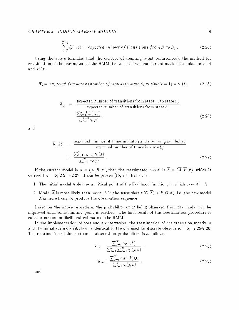
CHAPTER 2. HIDDEN MARKOV MODELS 16T�1Xt=1 �t(i; j) = expected number of transitions from Si to Sj : (2:24)Using the above formulas (and the concept of counting event occurrences), the method forreestimation of the parameters of the HMM, i.e. a set of reasonable reestimation formulas for �, Aand B is:�i = expected frequency (number of times) in state Si at time(t = 1) = 1(i) ; (2:25)aij = expected number of transitions from state Si to state Sjexpected number of transitions from state Si= PT�1t=1 �t(i; j)PT�1t=1 t(i) ; (2.26)and bj(k) = expected number of times in state j and observing symbol vkexpected number of times in state Sj= PTt=1;Ot=vk t(j)PTt=1 t(j) : (2.27)If the current model is � = (A;B; �), then the reestimated model is � = (A;B; �), which isderived from Eq 2.25 - 2.27. It can be proven [15, 73] that either:1. The initial model � de�nes a critical point of the likelihood function, in which case � = �.2. Model � is more likely than model � in the sense that P (Oj�) > P (Oj�), i.e. the new model� is more likely to produce the observation sequence.Based on the above procedure, the probability of O being observed from the model can beimproved until some limiting point is reached. The �nal result of this reestimation procedure iscalled a maximum likelihood estimate of the HMM.In the implementation of continuous observation, the reestimation of the transition matrix Aand the initial state distribution is identical to the one used for discrete observation Eq. 2.25-2.26.The reestimation of the continuous observation probabilities is as follows:cjk = PTt=1 t(j; k)PTt=1PMk=1 t(j; k) ; (2:28)�jk = PTt=1 t(j; k)OtPTt=1 t(j; k) ; (2:29)and

CHAPTER 2. HIDDEN MARKOV MODELS 17Ujk = PTt=1 t(j; k)(Ot � �jk)0(Ot � �jk)PTt=1 t(j; k) : (2:30)Where t(j; k) is the probability of being in state j at time t with the kth mixture componentaccounting for Ot, i.e., t(j; k) def= " �t(j)�t(j)PNi=1 �t(i)�t(i#" cjkP (Ot; �jk;Ujk)PMm=1 cjmP (Ot; �jm;Ujm)# : (2:31)This term can be generalized to t(j) in the case of a simple mixture, i.e. M = 1, and rewrittenexactly as in Eq. 2.21. The second term in the de�nition of Eq. 2.31 is identically 1.2.6.2 The segmental K-means algorithmThe segmental K-means [62] starts with a training set of observations (the same as is required forparameter estimation), and an initial estimate of all model parameters. Following model initializa-tion, the set of training observation sequences is segmented into states, based on the current model�. This segmentation is achieved by �nding the optimum state sequence, via the Viterbi algorithm,and then backtracking along the optimal path. The observation vectors within each state Sj areclustered into a set ofM clusters, where each cluster represents one of theM mixtures of the bj(Ot)density. From the clustering, an updated set of model parameters is derived as follows:� cjm - The number of vectors classi�ed in cluster m of state j divided by the number of vectorsin state j.� �jm - The sample mean of the vectors classi�ed in cluster m of state j.� Ujm - The sample covariance matrix of the vectors classi�ed in cluster m of state j.Based on this state segmentation, updated estimates of the aij coe�cients may be obtained bycounting the number of transitions from state i to j and dividing it by the number of transitions fromstate i to any state (including itself). If the number of mixtures (M) is one, then the computationof these values is simpli�ed.An updated model � is obtained from the new model parameters and the formal reestimationprocedure is used to reestimate all model parameters. The resulting model is then comparedto the previous model (by computing a distance score that re ects the statistical similarity ofthe HMMs, based on the probability functions of the parameters). If the model distance scoreexceeds a threshold, then the old model � is replaced by the new (reestimated) model �, andthe overall training loop is repeated. If the model distance score falls bellow the threshold, thenmodel convergence is assumed and the �nal model parameters are saved. The convergence of thisalgorithm is also assured [48] as is in the Baum-Welch algorithm.2.7 Clustering techniques used in HMMBoth the Baum and the segmental K-means algorithms are initialized with an initial model �start.This initialization is crucial to the results of the algorithms due to the locality problems of the above

CHAPTER 2. HIDDEN MARKOV MODELS 18mentioned algorithm. The computation of the initial model is usually carried out by a clusteringalgorithm. Clustering of data is the process of partitioning a given set of data samples into severalgroups [22, 38, 12, 47]. Each group usually indicates the presence of a distinct category in the data.One of the common clustering algorithms is de�ned as follows:1. set n = 12. Choose some initial values for the model parameters - �(n)1 ;�(n)2 � � � ;�(n)K , where K is thenumber of clusters computed. Each of these �j represents one class of the algorithm, andincludes the parameters characterizing that class.3. Loop: classify all the samples, by assigning them to the class of the closest divergence. Thisclassi�cation de�nes an error measure, which is the total divergence of all the samples fromtheir matched classes.4. Recompute the model parameters as the average of all the samples in their class. The newset of parameters is �(n+1)1 ;�(n+1)2 � � � ;�(n+1)K5. If the distance between the error measures of sets �(n+1)j and �(n)j is below some threshold,stop, and the result is �(n)j .6. n ! n + 17. go to beginning of Loop (step 3).This algorithm is sometimes referred to as the K-means algorithm [22, 49], where K stands forthe number of clusters sought. Other names for this algorithm are the LBG [47], the ISODATAalgorithm [22] or VQ (Vector Quantization) algorithm. The algorithm described above is referredto as hard clustering, due to the fact that each data point is related to one cluster. There exists,however, a di�erent clustering method referred to as soft clustering, in which each data point isrelated to all of the centroids, each with a certain probability. In this work the soft clusteringtechnique was used.2.7.1 KL-divergenceThe process of clustering data samples necessitates a divergence measure, which is used whenclassifying each data sample to the matching cluster (step No. 3 in the K-means algorithm). Anoptimal measure for the case of known observation probabilities is shown below.For a given multidimensional process the probabilities are q1; q2 � � � ; qK, where qi may form anydistribution function. The observation of this process is n1; n2; � � � ; nK from any symbol space. Inorder to classify the observation vector, its probabilityP (n1; n2; � � � ; nK jq1; q2; � � � ; qK) ; (2:32)is computed. Regarding this observation as the output of N Bernoulli trials, whereN = KXi=1 ni ; (2:33)

CHAPTER 2. HIDDEN MARKOV MODELS 19the probability measure of Eq. 2.32 is:P (n1; n2; � � � ; nKjq1; q2; � � � ; qK) = N !QKi=1 ni! KYi=1 qnii : (2:34)Taking the natural logarithm of both sides, and using Stirling's approximation, i.e.N ! � p2�N�Ne �N ; (2:35)we get:logP (njq) = N log(N)�N �Xi ni log(ni) +Xi ni +Xi ni log(qi) + o(N) = (2:36)(due to Eq. 2.33) = N log(N)�Xi ni log(ni) +Xi ni log(qi) + o(N) : (2:37)De�ning a new set of observations pi as:pi def= niN ; (2:38)Eq. 2.37 can be rewritten as:�Xi ni log�niN�+Xi ni log(qi) + o(N) = �N "Xi pi log�piqi�# + o(N) : (2:39)The probability measure of Eq. 2.32 can be written as:P (njq) � e�ND[pjjq] ; (2:40)where D[pjjq] is de�ned as: D[pjjq] def= XAllx p(x)log�p(x)q(x)� : (2:41)This expression is called the Kullbak-Liebler divergence measure (KL) [45]. It is also sometimesreferred to as the cross-entropy of the distributions [48].A di�erent way of reaching the same divergence measure is by using Bayes rule. Suppose thattwo hypotheses exist concerning the distribution of data:1. H1: The data are distributed according to P (x(n)jH1).2. H2: The data are distributed according to P (x(n)jH2).

CHAPTER 2. HIDDEN MARKOV MODELS 20In the context of clustering problems these hypotheses are the di�erent centroids of the clusters,and the problem is to classify a given observation x to one of the centroids.Given n independent samples from one of the distributions, the task is to evaluate the termP (H1jx(n)) which is, according to Bayes' rule:P (x(n)jH1)P (H1)P2i=1 P (Hi)P (x(n)jHi) ; (2:42)because the samples are independent, the probability can be turned into a multiplication:P (x(n)jHi) = nYj=1P (xj jHi) : (2:43)Thus the term in 2.42 can be rewritten as:P (H1jx(n)) = P (H1)Qnj=1 P (xj jH1)P2i=1 P (Hi)Qnj=1 P (xj jHi) : (2:44)By dividing the nominator and denominator by the same expression we get:P (H1jx(n)) = 11 + P (H2)P (H1 Qnj=1 P (xjjH2)P (xjjH1) = (2:45)= 11 + elog�P (H2)P (H1 Qnj=1 P (xj jH2)P (xj jH1)� = (2:46)= 11 + elog�P (H2)P (H1)�+Pnj=1 log�P (xj jH2)P (xj jH1)� : (2:47)Due to the fact that P (H1) and P (H2) do not depend upon the data samples, the logarithm oftheir portion could be written as a constant �. Thus, 2.47 can be rewritten as:11 + e�Pnj=1 log�P (xj jH1)P (xj jH2)��� = 11 + e�X ; (2:48)where X = nXj=1 log P (xj jH1)P (xj jH2)!+ � : (2:49)According to the strong law of large numbers, the sample average converges to the expectedvalue with respect to the distribution which the data were taken from (assuming that the data weretaken from H1), thus indicating that as the summation factor grows this expression becomes:X = n XAll x p(xjH1)log�P (xjH1)P (xjH2)�� � : (2:50)

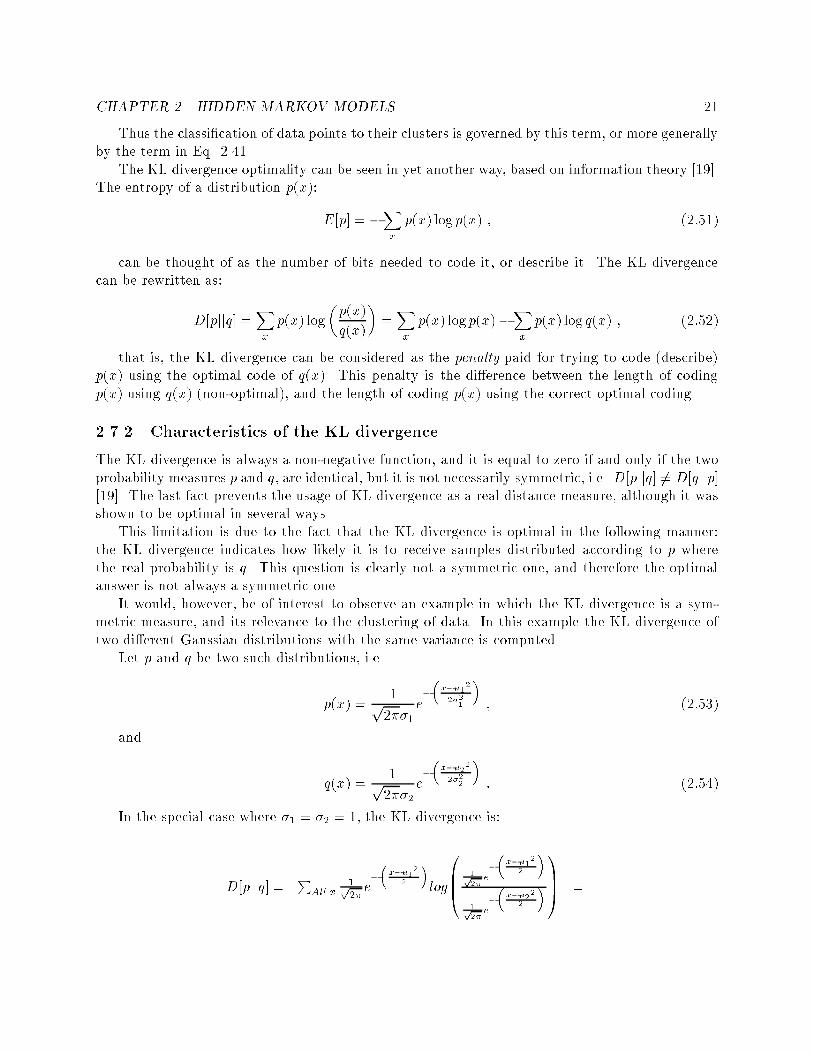
CHAPTER 2. HIDDEN MARKOV MODELS 21Thus the classi�cation of data points to their clusters is governed by this term, or more generallyby the term in Eq. 2.41.The KL divergence optimality can be seen in yet another way, based on information theory [19].The entropy of a distribution p(x): E[p] = �Xx p(x) log p(x) ; (2:51)can be thought of as the number of bits needed to code it, or describe it. The KL divergencecan be rewritten as:D[pjjq] =Xx p(x) log�p(x)q(x)� =Xx p(x) log p(x)�Xx p(x) log q(x) ; (2:52)that is, the KL divergence can be considered as the penalty paid for trying to code (describe)p(x) using the optimal code of q(x). This penalty is the di�erence between the length of codingp(x) using q(x) (non-optimal), and the length of coding p(x) using the correct optimal coding.2.7.2 Characteristics of the KL divergenceThe KL divergence is always a non-negative function, and it is equal to zero if and only if the twoprobability measures p and q, are identical, but it is not necessarily symmetric, i.e. D[pjjq] 6= D[qjjp][19]. The last fact prevents the usage of KL divergence as a real distance measure, although it wasshown to be optimal in several ways.This limitation is due to the fact that the KL divergence is optimal in the following manner:the KL divergence indicates how likely it is to receive samples distributed according to p wherethe real probability is q. This question is clearly not a symmetric one, and therefore the optimalanswer is not always a symmetric one.It would, however, be of interest to observe an example in which the KL divergence is a sym-metric measure, and its relevance to the clustering of data. In this example the KL divergence oftwo di�erent Gaussian distributions with the same variance is computed.Let p and q be two such distributions, i.e.p(x) = 1p2��1 e��x��122�21 � ; (2:53)and q(x) = 1p2��2 e��x��222�22 � : (2:54)In the special case where �1 = �2 = 1, the KL divergence is:D[pjjq] = PAll x 1p2� e��x��122 �log0BB@ 1p2� e��x��122 �1p2� e��x��222 �1CCA =

CHAPTER 2. HIDDEN MARKOV MODELS 22= PAll x 1p2�e��x��122 � �22��21�2x�2+2x�12 == �22�2�1�2��21+2�212 == (�1��2)22 : (2.55)The KL divergence in this example is the Euclidean distance measure. That is, in the case of twonormal distributions, the optimal divergence between them is the commonly used distance measure.2.8 Hidden Markov Model of multivariate Poisson probabilityobservationThe notion of Poisson probability is introduced here by means of completeness of description ofdata modeling. One of the common assumptions regarding the probability distribution of spiketrains is the Poisson distribution: P�(n) = e���nn! : (2:56)That is, the probability of �nding a certain number of spikes (n) in some interval is governedby this probability function with a mean of �. Throughout this section, � will be referred to as the�ring rate of cells.Under the Poissonian distribution the clustering divergence measure will be shown, and a simpleML estimation of parameters will be reached.2.8.1 Clustering data of multivariate Poisson probabilityThe divergence was computed on the basis of the assumption that the �ring rate followed anuncorrelated multivariate Poisson process:P (n1; n2; � � � ; ndj�) = dYi=1 e��i�niini! ; (2:57)where � = (�1; �2; � � ��d) and d is the number of uncorrelated Poisson processes. For 1-dimensional Poisson distribution (d = 1), the divergence is given by:D[pjjq] =Xx p(x) log p(x)q(x) =Xx e��1�x1x! log e��1�x1x!e��2�x2x! = �2 � �1 + �1 log �2�1 ; (2:58)where p(x) = e��1�x1x! ; (2:59)and q(x) = e��2�x2x! : (2:60)The uncorrelated multivariate divergence is simply the sum of divergences for all the 1-dimensionalprobabilities.

CHAPTER 2. HIDDEN MARKOV MODELS 23This multivariate Poisson divergence is not a symmetric measure, i.e. D[pjjq] 6= D[qjjp]. Thusin Eq. 2.58, �1 is the �ring rate of the sample vector and �2 is the �ring rate of the centroid ofthe cluster checked. The KL divergence measures the probability of assigning a �ring rate vector(from the data) to a speci�c centroid.2.8.2 Maximum likelihood of multivariate Poisson processA derivation of ML estimate of multivariate Poisson process with a pair-wise cross-correlation willbe shown here. The probability of an observation vector n is de�ned as:P (nj�; ~�) def= NYi=1 e��i�niini! exp[� NXi=1 NXj=1�ijninj ] 1Z ; (2:61)where �i is the vector of �ring rates of the multivariate Poisson distribution (as described inthe previous subsection), �ij is the cross-correlation matrix indicating the correlation between theprocess i and the process j, and Z is de�ned as:Z(�; ~�) def= M1Xn1=1 M2Xn2=1 � � � MNXnN=1P (nj�; ~�) : (2:62)Mi is de�ned as the minimal value which satis�esMiXj=1 e��i�jij! < � 8�i 2 � : (2:63)The log likelihood function of this process islog$(n(T )) = TXt=1 log P (ntj�; ~�) = TXt=1(( NXi=1 logP�i(ni))� ( NXi=1 NXj=1;i>j �ijninj)� Tlog(Z)) : (2:64)The ML is computed by satisfying the terms@ log$@�i = 0; @ log$@�ij = 0 : (2:65)This ML computation results in@ log$@�i = (PTt=1 nti�i )� T � TZ PM1n1=1;PM2n2=1; � � � ;PMNnN=1[(QNj=1;j 6=i e��j�njjnj ! )(exp[PNj=1PNk=1;j>k ��jknjnk ])( 1ni!e��i�ni�1i )]= 0 ; (2.66)and

CHAPTER 2. HIDDEN MARKOV MODELS 24@ log$@�ij = (PTt=1�ntintj)� TZ PM1n1=1;PM2n2=1; � � � ;PMNnN=1[(QNk=1 e��k�nkknk! )(exp[PNk=1PNl=1��klnknl])(�ninjexp[��ijninj ])]= 0 : (2.67)Eq. 2.66 2.67 can be solved using any gradient descent, such as conjugate gradient methods, see[59, pages 254{259].

Part IIModel Implementation

25

Chapter 3Physiological Data and PreliminaryAnalysis3.1 Frontal cortex as a source of dataThe aim of the research presented here, was to apply HMM models to physiological data in orderto be able to predict cognitive states of the organism. One of the valuable sources of informationabout the activities of the brain is the frontal cortex (FC), which is located in the anterior thirdof the brain. The FC is known to contain high association areas, i.e. areas which are not directlyconnected to sensory or motor systems, but receive connections from, and send connections to, manyother cortical areas. The FC has been divided into three broad regions: the motor cortex (MC),the premotor cortex (PMC) and the prefrontal cortex (PFC). Two of these areas were investigatedin this work, the PMC and PFC [33, 56]. Fuster claims that "the PFC is critical for temporalorganization of behavior. It mediates cross-temporal sensorimotor contingencies, integrating motoraction (including speech in humans) with recent sensory information" [26, 27, 28]. This area is alsoinvolved in the composition and execution of plans [18]. The PMC is essential for the preparationof movement and the ability to develop an appropriate strategy for movement [33]. These areas arecharacterized by multiple connections with many other cortical areas, most of which are associativeareas.Information about neural activity in the FC is gained through electrophysiological recording ofcells in a behaving animal (a conscious animal engaged in a speci�c pre-de�ned task) [26, 70]. Thisenables us to compare the recordings of cells to the actual activity of the animal. A pre-de�nedtask that is sometimes used when recording from the PMC and the PFC is the spatial delayedresponse task [52, 53, 51, 25]. This task consists of the following stages:1. Initialization of task.2. A sensory cue.3. Delay period.4. An action cue.5. Motor response contingent on the cue. 26

CHAPTER 3. PHYSIOLOGICAL DATA AND PRELIMINARY ANALYSIS 276. Reward in the case where the response was correct.It is known that both areas under investigation (PMC and PFC), play an important role in theperformance of this task.3.2 Description of physiological experimentThe data used in the present analysis were collected in the Higher brain function laboratory atthe Hadassah Medical School. The present chapter describes the experiments carried out there,and the following chapter will discuss the application of the model to these data. Recordings weretaken from two Rhesus monkeys (Macaca Mulatta), trained to perform a spatial delayed-responsetask. The experiments were conducted by Y. Prut, I. Halman and H. Slovin as part of their Ph.Dwork under the supervision of M. Abeles, H. Bergman and E. Vaadia.3.2.1 Behavioral modes of the monkeyThe monkeys were trained to perform a spatial task, in which they had to alternate between twobehavioral modes. The monkey initiated the trial by pressing a central key, and a �xation light wasturned on in front of it. Then, after 3-6 seconds, a visual stimulus appeared, in the form of a cuelight, either on the left or on the right. The stimulus was presented for 100 ms. The stimulus wasfollowed by a delay period of 1-32 seconds, in factors of 2 (i.e. 1,2,4,8,16,32 seconds). Following thedelay period, the �xation light was dimmed, and the monkey was required to touch the visual cuelight (\Go" mode), or keep its hand on the central key regardless of the external stimulus (\No-Go"mode). The monkey was rewarded for the correct behavior with a drop of juice. After 4 correcttrials, all the lights in front of the monkey blinked, signaling to the monkey to change its behavioralmode - so that if it had started in the \Go" mode it now had to switch to \No-Go" mode, and viceversa. A diagram of the behavioral modes is presented in �gure 3.1.The training period for each monkey lasted 2-4 months. At the end of the training, the monkeyswere able to perform this complicated task with low error rates (around 10%).3.2.2 Data from recording sessionAt the end of the training period, the monkeys were prepared for electrophysiological recording.Surgical anesthesia was induced. A recording chamber was �xed above a hole drilled in the skull toallow for a vertical approach to the frontal cortex. After recovery from surgery, recording sessionsbegan, and the activity of the cortex was recorded while the monkey was performing the previously-learned routine. Each recording session was held on a separate day, and typically lasted 2-4 hours.During each of the recording sessions, six microelectrodes were used simultaneously. The electrodeswere placed in a circle with a radius of 0.5 mm. With the aid of two pattern detectors and fourwindow-inscriminates, the activity of up to 11 single cells (neurons) was concomitantly recorded[68, 4]. This activity consists of the discrete times of action potentials of the cells, referred to asthe spike train of the cell. The recorded data includes the following information:1. The spike trains of all the cells.2. The recording session events. These events are either the stimuli presented to the monkey orthe responses of the monkey.

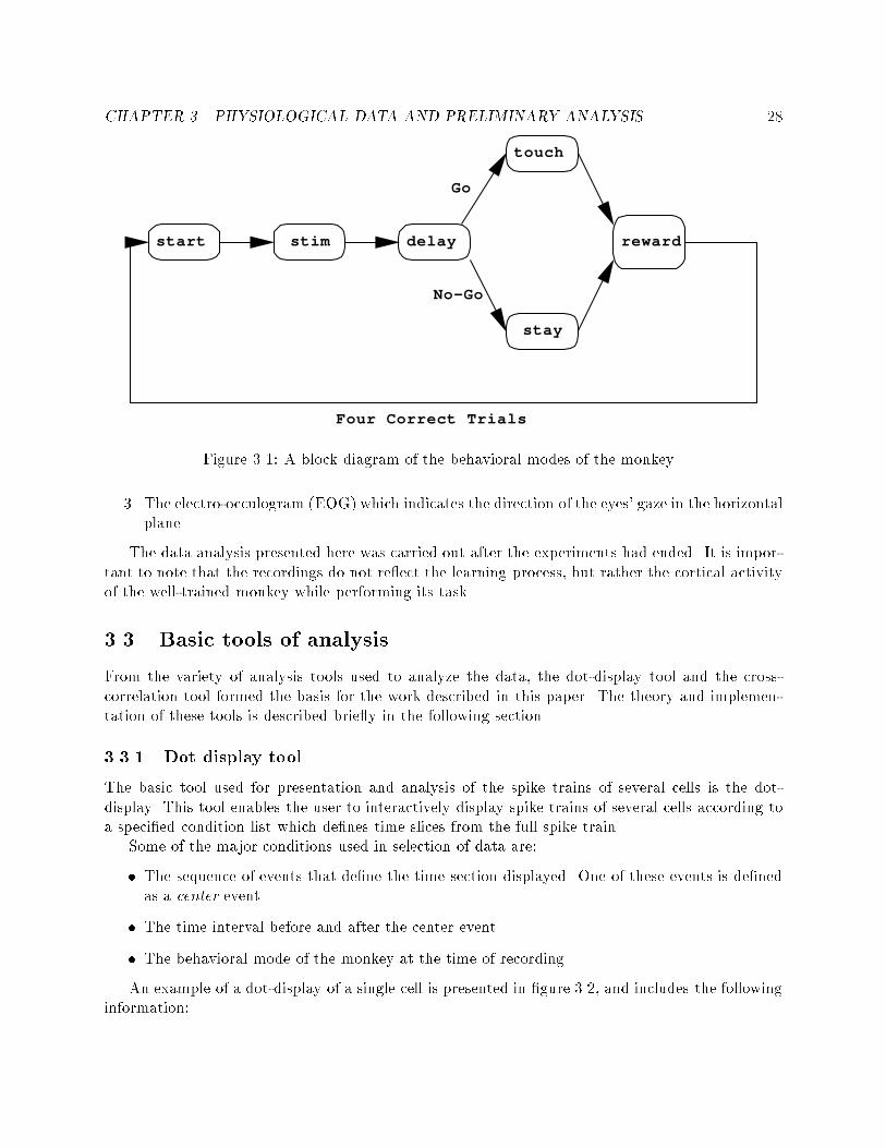
CHAPTER 3. PHYSIOLOGICAL DATA AND PRELIMINARY ANALYSIS 28start stim delay

Go

No−Go

stay

touch

reward

Four Correct TrialsFigure 3.1: A block diagram of the behavioral modes of the monkey.3. The electro-occulogram (EOG) which indicates the direction of the eyes' gaze in the horizontalplane.The data analysis presented here was carried out after the experiments had ended. It is impor-tant to note that the recordings do not re ect the learning process, but rather the cortical activityof the well-trained monkey while performing its task.3.3 Basic tools of analysisFrom the variety of analysis tools used to analyze the data, the dot-display tool and the cross-correlation tool formed the basis for the work described in this paper. The theory and implemen-tation of these tools is described brie y in the following section.3.3.1 Dot display toolThe basic tool used for presentation and analysis of the spike trains of several cells is the dot-display. This tool enables the user to interactively display spike trains of several cells according toa speci�ed condition list which de�nes time slices from the full spike train.Some of the major conditions used in selection of data are:� The sequence of events that de�ne the time section displayed. One of these events is de�nedas a center event.� The time interval before and after the center event.� The behavioral mode of the monkey at the time of recording.An example of a dot-display of a single cell is presented in �gure 3.2, and includes the followinginformation:

CHAPTER 3. PHYSIOLOGICAL DATA AND PRELIMINARY ANALYSIS 29� Cell index.� Spike trains of the speci�ed cell, drawn one on top of the other. Each one of the spikes in thespike train is presented as a small vertical line.� The number of spike trains drawn - in this example there are 233 spike trains.� The sequence of events de�ning the selection criteria for the spike trains.� The recording session data are divided into separate �les, and the list of �les used for thisdisplay is shown.� The time scale is shown on the abscissa. This example presents spike trains from 4000 msbefore the center event, until 5000 ms after that event.The peri-stimulus-time (PST) histogram is drawn above the spike trains. In this example, abin width of 50 ms was used, i.e. in the 9000 ms presented in this �gure, 180 such bins exist. Thecomputation process involves counting the spikes in each such bin and dividing the result by thenumber of repetitions for each bin. The result is transformed into units of spikes-per-second bydividing it by the time duration of the bins. The histogram is automatically scaled according tothe maximum �ring rate value, which is given on the upper left side of the histogram, in units ofspikes-per-second. In this example, the maximum �ring rate is 4 spikes-per-second.3.3.2 Temporal cross correlation toolThe temporal cross-correlation function between cells measures the correlation between spike trainsof cells (discrete events), and can be computed in bins of variable length. The �gures representingthe cross-correlation function with a speci�c bin width will henceforth be called a cross-correlograms[69].The temporal cross-correlogram between two cells i and j at time bin l is de�ned as follows:Rij(l) = 1Nt�t NtXt=1S 0i(t)S 00j (t + l) : (3:1)Where S 0i(t) is the event that cell i emitted a spike in the time bin (t; t+ 0:001), and S 00j (t+ l)is the event that cell j emitted a spike in the time bin (t + l�t; t+ (l+ 1)�t). The absolute timementioned above is in seconds, i.e. 0.001 is 1 ms. Nt is the number of spikes of cell i (that areused as \triggers" for the averaging) and �t is the time bin width. Where l�t extends from -T to+T , the cross-correlation functions for positive l�t values (0 < l�t < T ) express the average �ringrate of cell j at time l�t, given that cell i �red a spike at time 0. Similarly, the cross-correlationfunction at (�T < l�t < 0) gives the �ring rate of cell i, given that cell j �red a spike at time 0.The shape of the cross-correlogram provides indications for the functional connectivity betweenneurons. Typical shapes of cross-correlograms feature peaks or troughs near the origin. When thepeaks or troughs extend to both sides of the origin, they are usually interpreted as re ecting a sharedinput to the two neurons. Narrow peaks or troughs, restricted to one side of the cross-correlogram,are usually interpreted as re ecting a direct synaptic interaction.An example of a cross-correlogram is presented in �gure 3.3, and includes the following infor-mation:

CHAPTER 3. PHYSIOLOGICAL DATA AND PRELIMINARY ANALYSIS 30 6

0 5000-4000

4cl85b.011-129 (qual:3) SEQ: [1]*[23,25]*[33,35]

TRIGS = 233

Cell Index

Time before Time After

Firing Rate Histogram

Select SequenceFile ListFiring Rate Scale

Spike trainsRepetition NumberMillisec Millisec

(Hz)

Figure 3.2: An example of a dot-display.� The indexes of the cells used to compute the correlogram.� The average �ring rate of each cell.� The time scale of the cross-correlogram is shown on the abscissa. In this example, from -500ms to +500 ms� The �ring rate is shown on the ordinate in units of spikes-per-second.� The total duration of spike trains used to compute this correlogram.� Bin size of Gaussian smoothing applied to the counting of the correlation function.� An average line which is the average of the second cell.

CHAPTER 3. PHYSIOLOGICAL DATA AND PRELIMINARY ANALYSIS 31I:BL16A.006 I:BL16A.100 EXTERNAL FILE TYPE = 2 REGULAR T= 412. S BIN= 10.0

3 TO 5 RT = 0.95/S RC = 0.39/S L= 230

AVRG1= 0.05/BN AVRG2= 0.11/BN HISPK= 3.08/S TIMPK= 10.00mS

-5 -4 -3 -2 -1 0 1 2 3 4 5 TIME MSEC X10 2

0

62

124

186

248

310

SP

IKE

S/S

EC

X

10

-2

CROSS INTENSITY HISTOG.043 / 67

ZNAV

Bin Size

Measurement

duration

Average Line Significance Line

first cell firing rate

second cell firing rate

Cells Indexes

Figure 3.3: An example of a cross-correlation function (correlogram) of two cells.� Signi�cance lines with a con�dence level of 0.005 for each side of the average, computed onthe tails of the correlation function, i.e. from -500 to -400 ms, and from +400 to +500 ms.3.4 Quality of cells recordedThe quality of the recording is parameterized in several di�erent non-overlapping ways. Theseparameters are:1. The isolation score given to a cell during a recording session.2. The stationarity of the cell as measured afterwards on the dot-display of the cell.3. The �ring rate of the cell.4. The tendency of the cell to change its �ring rate in response to events.These parameters were integrated into a total score.3.4.1 Isolation score given to cells during recording sessionThe �rst parameter is the isolation score that each cell is given during the recording session. Thisscore is evaluated by the experimenter based on the percentage of spikes falling within a threshold

CHAPTER 3. PHYSIOLOGICAL DATA AND PRELIMINARY ANALYSIS 32of probability, inside the window discriminator. The scores are:A : Very well isolated single neuron with a large, unmistakable spike.B : Most of the time a well isolated single neuron can be identi�ed, but occasionally a spike fromanother cell may intrude.B- : The same as B, but some of the spikes are lost due to thresholds in the spike sorters.C+ : Two neurons, but most of the spikes originate from one neuron.C : Two neurons which cannot be observed separately.C- : Most of the time two neurons are counted, but occasionally other neurons are counted as well.D : More than two neurons together.E : Many small neurons - with much background noise.Cells of types A and B are sure to be single, well isolated neurons, varying only in the shape oftheir spikes. The other types should be used, therefore, with caution.Cells are given isolation scores several times during each recording session, due to the fact thatthese scores may vary over time. For a cell to be of use, it is usually required to remain withina small variance of score values. While recording the activity of the cells there are other types ofquality indications:� The reliability of the discrimination between cells.� Which cells tend to contaminate one another.� The pattern of the spike activity.This information is also taken into account when the cells are chosen, but in a more qualita-tive way. For example two cells of type C were not used, if they were recorded from the sameelectrode, and the experimenter noted that they tended to contaminate one another, because thiscontamination may cause a severe artifact in their cross-correlation function.3.4.2 Stationarity of a cellAnother measure of the acceptability of cells for analysis, is their stationarity during the recordingsession. This measure is extracted from the data after the recording session is over. Nonstationaritymay be due to a non-stable recording - a recording of a cell that was injured, for example. Aninjury to a cell may have occurred while the electrodes were penetrating the tissue, and so the spiketrain of this cell would not be reliable. Instability may also result from a small movement in thetissue recorded. Another possible reason for nonstationarity may be an actual nonstationarity inthe cell activity.An example of nonstationarity may be seen in �gure 3.4. In this �gure, a cell that was givenan isolation score of B is shown. Although this is a high isolation score, it can be seen clearly thatthe cell changes its �ring rate dramatically during the recording session. This dramatic changeprecludes the use of all the cell spike trains as a basis for further analysis. It is possible to use

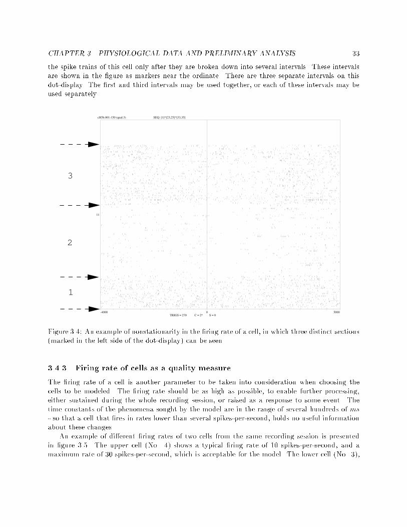
CHAPTER 3. PHYSIOLOGICAL DATA AND PRELIMINARY ANALYSIS 33the spike trains of this cell only after they are broken down into several intervals. These intervalsare shown in the �gure as markers near the ordinate. There are three separate intervals on thisdot-display. The �rst and third intervals may be used together, or each of these intervals may beused separately.11

0 5000-4000

cl85b.001-150 (qual:3) SEQ: [1]*[23,25]*[33,35]

TRIGS = 270 C = 2* S = 0

1

2

3

Figure 3.4: An example of nonstationarity in the �ring rate of a cell, in which three distinct sections(marked in the left side of the dot-display) can be seen.3.4.3 Firing rate of cells as a quality measureThe �ring rate of a cell is another parameter to be taken into consideration when choosing thecells to be modeled. The �ring rate should be as high as possible, to enable further processing,either sustained during the whole recording session, or raised as a response to some event. Thetime constants of the phenomena sought by the model are in the range of several hundreds of ms- so that a cell that �res in rates lower than several spikes-per-second, holds no useful informationabout these changes.An example of di�erent �ring rates of two cells from the same recording session is presentedin �gure 3.5. The upper cell (No. 4) shows a typical �ring rate of 10 spikes-per-second, and amaximum rate of 30 spikes-per-second, which is acceptable for the model. The lower cell (No. 3),

CHAPTER 3. PHYSIOLOGICAL DATA AND PRELIMINARY ANALYSIS 34however, is �ring at a much lower rate - its maximum rate is 0.5 spikes-per-second. This low �ringrate, combined with a lack of speci�c responses, precludes the use of this cell in the model. 3

4

0 5000-4000

30bl16a.001-100 (qual:3) SEQ: [1]*[20]*[33,35]

TRIGS = 195 C = 2* S = 0Figure 3.5: An example of di�erent �ring rates of two cells from the same recording session.3.4.4 Responsiveness of cells to eventsModulation of �ring rates around objectively measurable events is one of the important factorstaken into consideration when scoring a cell. The signi�cance of responsiveness depends on themodel of information-processing in the cortex. If the model puts the emphasis on the �ring rates ofthe cells, then the change in the �ring rate would be considered evidence for response to events. Ifthe model emphasizes exact temporal structures of a series of spikes, than this temporal structurewould be considered a key to the responsiveness of cells. The present research uses the �rst modelas a basis for measuring responsiveness.Figure 3.6 shows the activity of two cells whose spike trains were gathered from the samerecording session, near the same external cue. The lower cell (No. 5) shows a prominent responseto the external stimulus. The external stimulus in this example was the cue given to the animal(either from the right or from the left), as part of the behavioral mode described in �gure 3.1.

CHAPTER 3. PHYSIOLOGICAL DATA AND PRELIMINARY ANALYSIS 35The cue of every trial is used here as time 0. The changes in the �ring rate of this cell matchthe di�erent delay times (1,2,4,8 seconds) after the cue, at which the "Go" signal was presented.Furthermore, it can be seen in the dot-display that the response is characterized by a steep riseand a slow decay. The upper cell (No. 15) on the other hand, shows only a very weak response tothe stimulus. 5

15

0 9000-1000

23bl39a.001-80 (qual:3) SEQ: [1]*[20]*[33,35]

TRIGS = 161 C = 2* S = 3*Figure 3.6: An example of two cells that show di�erent responses to the same stimulus.

Chapter 4Application of the Model4.1 Data selection stageThe data used for modeling came from the recording sessions of 2 monkeys. The behavioralparadigm performed by the monkey in all the recording sessions was the Delayed Release Paradigmpresented in �gure 3.1 (Chapter 3 Section 2). The data used in the modeling included only thespike trains of all the cells recorded throughout each recording session. A quality check was carriedout for each recording session separately, according to the following stages:1. Only cells that were given isolation scores equal to or higher than C in the recording session(see Chapter 3 Section 4) were used.2. The isolation score of the cell had to be stable over time. If that score was not stable duringthe whole session, stable intervals of the session were chosen.3. Only stationary cells were used (see Chapter 3 Section 4). The stationarity check was per-formed using the dot-display tool. If the cells were not stationary during the whole session,only stable intervals of the session were chosen.4. Cells recorded from the same electrode were checked for contamination evidence (see Chapter3 Section 4), if any existed, at least one of these cells was not used.5. The �ring rate of the cell had to be higher than several spikes-per-second. The threshold usedwas 1 spike-per-second. It was not necessary that the average �ring rate exceed the threshold,and is was considered su�cient if the �ring rate of the cell exceeded the threshold only in afew sections of the spike trains, e.g. near some external stimulus, averaged throughout thewhole recording session.This quality check was applied to 8 recording sessions, out of which 6 were found to includesu�cient data for further processing. Su�cient data in this context was de�ned as follows:1. More than 5 well isolated cells.2. The intervals chosen held more than 5000 seconds of stable isolation scores and stationaryrecording. 36

CHAPTER 4. APPLICATION OF THE MODEL 37Following the quality check, the data were divided into trials made in the \Go" mode and the \No-Go" mode. From this point onwards, the spike trains of these behavioral modes were processedseparately. The result of this selection can be seen in table 4.1.Session Cells States \Go" Length \No-Go" Length Total Record Length Areabl16 8 6 3907 4097 8004 PMCbl25 8 7 6202 5131 11333 PMCbl29 8 8 2557 2508 5065 PMC-MCbl39 6 7 5987 5864 11854 PMCcl77 6 6 9946 6566 16512 PFCcl85 8 6 3908 4654 8562 PFCTotal 44 40 32507 28820 61327Table 4.1: Presentation of the recording sessions used throughout the experiments. For eachrecording session, the number of well-isolated cells used is indicated, as is the total length of thesession (in seconds) and the cortical area from which the data were recorded. These time tablesare presented separately for the \Go" mode and the \No-Go" mode.It is important to note that the cells were not chosen according to any criterion of responsiveness- some of the cells chosen were responsive to an external stimulus and some showed only weakresponses to the stimulus.4.2 Computation of parameters used in the modelThe model assumes that the spike trains are distributed according to a Poisson distribution [1].The distances between spikes are distributed exponentially and their number in each frame, n,depends only on the mean �ring rate �, through the distributionP�(n) = e���nn! : (4:1)The short-time �ring rate of the cell, which is the basic parameter of the multivariate Poissonprocess, was computed. The computation was done with a sliding window of 500 ms width, andwith transition of 100 ms. This computation transformed the day's �ring activity into a seriesof vectors, each N dimensional - where N is the number of cells in the experiment. An exampleof parameter computation is presented in �gure 4.1. This �gure presents a dot-display of 8 cells,recorded simultaneously. For each of these spike trains, the short-time �ring rate of the spike trainis plotted as a dashed line.In this example, a time scale of 4 seconds was used. This computation therefore produces 40vectors, each of them 8 dimensional. These vectors were the point-wise measurements for the nextstages of computation.

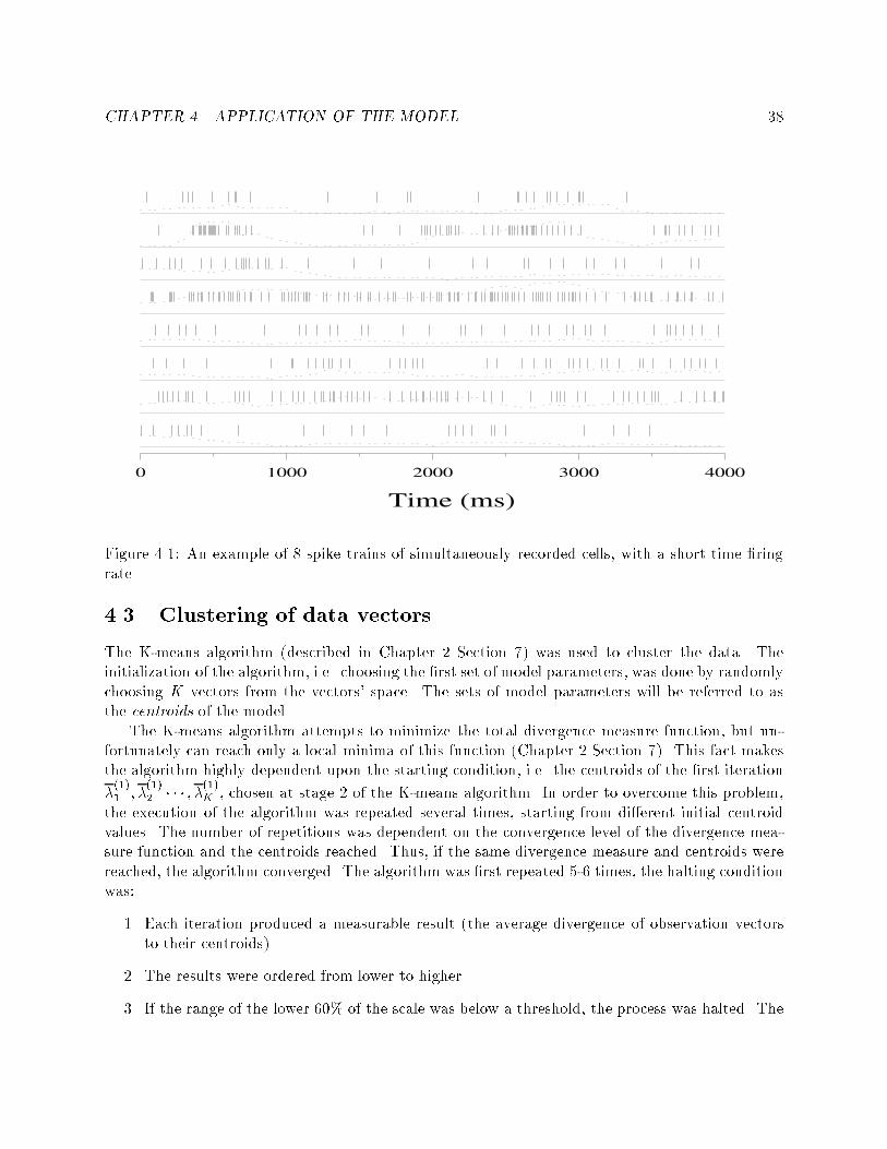
CHAPTER 4. APPLICATION OF THE MODEL 380 1000 2000 3000 4000

Time (ms)Figure 4.1: An example of 8 spike trains of simultaneously recorded cells, with a short time �ringrate.4.3 Clustering of data vectorsThe K-means algorithm (described in Chapter 2 Section 7) was used to cluster the data. Theinitialization of the algorithm, i.e. choosing the �rst set of model parameters, was done by randomlychoosing K vectors from the vectors' space. The sets of model parameters will be referred to asthe centroids of the model.The K-means algorithm attempts to minimize the total divergence measure function, but un-fortunately can reach only a local minima of this function (Chapter 2 Section 7). This fact makesthe algorithm highly dependent upon the starting condition, i.e. the centroids of the �rst iteration�(1)1 ; �(1)2 � � � ; �(1)K , chosen at stage 2 of the K-means algorithm. In order to overcome this problem,the execution of the algorithm was repeated several times, starting from di�erent initial centroidvalues. The number of repetitions was dependent on the convergence level of the divergence mea-sure function and the centroids reached. Thus, if the same divergence measure and centroids werereached, the algorithm converged. The algorithm was �rst repeated 5-6 times, the halting conditionwas:1. Each iteration produced a measurable result (the average divergence of observation vectorsto their centroids).2. The results were ordered from lower to higher.3. If the range of the lower 60% of the scale was below a threshold, the process was halted. The

CHAPTER 4. APPLICATION OF THE MODEL 39threshold used was 0.5.4. The algorithm was repeated 5 more times and all the results were checked beginning withstep No. 1.The number of clusters (K) used in the algorithm is �xed throughout one repetition. In orderto �nd the optimal number, several values were tested. For each of these values the algorithm wasrepeated several times, in order to reach convergence (as described above). The optimal number ofclusters was calculated based on the error measure functions for the di�erent values tested, takinginto consideration the number of clusters. As the number of clusters increases, the divergencemeasure is reduced, but it is necessary to �nd some balance between the two. This balance wascomputed based on the reduction rate: when the number of states is small this reduction is usuallylogarithmic, and when this number increases, this reduction rate becomes linear or less. The balancewas taken as the point where the change between logarithmic reduction rate and linear reductionrate occurs. An example of that process is shown in �gure 4.2. In this �gure two sections can beobserved:1. Number of states from 1 to 8, where the reduction is almost logarithmic.2. Number of states from 9 to 15, where the reduction is almost linear.The number of states used in this example was therefore 8. In order to classify each sample to aspeci�c centroid, a speci�c divergence measure is needed. This divergence was computed in Chapter2 Section 8, Eq. 2.58.An example of the execution of the clustering algorithm is shown in �gure 4.3. In this �gure,two executions of the K-means algorithm are shown. For each of them the error measure is shownas a function of the iteration of the algorithm. The data used for the two executions came fromdi�erent behavioral modes of the same recording session. The behavior shown in the graph istypical of this kind of algorithm: the �rst few iterations reduce the divergence measure functiondramatically and the last iterations are the \�ne tuning".This is a special case of a method called distributional clustering, recently developed in a moregeneral setup [67].4.4 Implementation of a full HMMThe next step in this framework was to compute a full Hidden Markov Model, consisting of thehidden states themselves and of the transition probabilities between them. In order to computethis model, the results of the clustering phase were used as initial conditions. These initial condi-tions included the number of states and their probability functions. Several values of a transitionmatrix were used for initialization of the algorithm. One of these values derived from the temporalsegmentation of the previous phase, and the others was chosen at random. All the elements inthe transition probabilities were non-zero, resulting in an ergodic model. The observations of themodeling were the �ring rate vectors, thus the model was computed for continuous observationswith one mixture each (Chapter 2 Section 2).The computation of the full Hidden Markov Model was carried out in two ways:

CHAPTER 4. APPLICATION OF THE MODEL 405

10

15

20

25

30

0 2 4 6 8 10 12 14 16

KL D

iverg

ence

Number of States

’likeli1’

Figure 4.2: An example of execution of a K-means algorithm for di�erent number of states, usingthe same data.1. Using the continuous observation Baum-Welch algorithm de�ned in Eq. 2.25 - 2.26 and 2.28- 2.30 (Chapter 2 Section 6).2. Using segmental K-means algorithm (described in Chapter 2 Section 6) using Eq. 2.12 - Eq2.18.The second method is less optimal than the �rst, but has been shown to produce similar resultsin other areas in which the HMM was used - automatic speech recognition, for instance [61].4.5 Insertion of �ring rate cross-correlations into the modelThe multivariate Poisson process is taken as a maximum entropy distribution with i.i.d. Poissonprior, subject to pair-wise channel correlations as additional constraints, yielding Eq. 2.61.The computation of the cross-correlation of the �ring rate was carried out using an iterativealgorithm based on Eq 2.66 - 2.67. This algorithm was based on the �rst stage of the model, i.e.without transition probabilities. The algorithm consisted of the following steps:1. Set n = 12. Choose initial values for the algorithm. These values are the �(n)i and �(n)ij .

CHAPTER 4. APPLICATION OF THE MODEL 418

9

10

11

12

13

14

15

16

17

0 10 20 30 40 50 60

KL

Div

erg

en

ce

Iterations

No-Go Mode dataGo Mode data

Figure 4.3: An example of execution of a K-means algorithm for two sets of data vectors.3. Beginning of loop.4. Compute the set �(n+1)ij from Eq 2.67 using the values of �(n)ij and �(n)i .5. Compute the set �(n+1)i from eq 2.66 using the values of �(n)ij and �(n)i .6. If the di�erence between the �(n)ij , �(n)i and �(n+1)ij , �(n+1)i is below a chosen threshold, stophere, and use the values �(n)ij , �(n)i as �nal values.7. n ! n + 1;8. Go to step No. 2.It was found that the full computation of Eq 2.66 - 2.67 was not feasible because of the numberof operations involved. The number of addition and multiplication operations at each iterationwas of the order of 1010. Furthermore, no analytical shortcut was found, due to the Poissonprobabilities (in contrast to the usual Gaussian distribution, in which the summation could bereplaced by integration). Another problem was that most of the elements outside the diagonal ofthe clusters' covariance matrix were very small. These two problems, when considered together,

CHAPTER 4. APPLICATION OF THE MODEL 42suggested that only the strongest cross-correlation element could be computed. That element waschosen according to the values in the covariance matrix of each cluster.The addition of the cross-correlation function, therefore, is limited to only one cross-correlationvalue per state.4.6 Search for correlation between state sequences and eventsOne of the main hypotheses was that it is possible to predict the actual events (stimulus to themonkey or behavioral action of the monkey) from the states computed by the model. Therefore,after the data had been labeled by the HMM, a check for sequences in the temporal segmentationwas carried out. This search, similarly to the process of constructing the whole model, was carriedout in an unsupervised manner, i.e. the information regarding the events was not inserted into thesearch algorithm.This search algorithm consisted of the following steps:1. A speci�c event E was chosen.2. The sequence of 3 states which followed this event closely in one of the trials was chosen andmarked as SQ.3. All the occurrences of sequence SQ were computed and marked on the data.4. The previously found sequence locations were compared to location of event E in the recordingsession, taking into consideration a possible delay of up to 100 ms between the event and thesequence. This comparison yielded the prediction of all other events of type E.Several di�erent events E were used and for each of them several sequences of states SQ wereutilized. The sequence of states examined in this algorithm, was made of three states (as indicatedin step No. 2). This is due to a preliminary examination, in which shorter sequences were used,but without any notable results.4.7 Display toolsAll the work described above was based on interactive tools, which enabled the research to checkand display graphically the following information:1. Spike trains of chosen cells.2. Firing rate vectors of the data.3. The clustering process (size of clusters, average divergence measure, etc.)4. The centroids of the di�erent models computed.5. The temporal segmentation of the data according to di�erent models.6. The segments' length distribution.In the research, a large amount of data was evaluated and these tools were used extensively inorder to assess the results reached and to direct the research in the most promising direction.

CHAPTER 4. APPLICATION OF THE MODEL 434.8 Temporal cross-correlation in di�erent statesThe temporal cross-correlation function was computed for all of the pairs of cells in all their di�erentstates. This computation was performed as follows:1. All the data from a recording session was segmented and labeled according to the full model(including transition probabilities).2. All the spike trains found in the segments of a given state were collected together.3. From the spike trains so selected, only segments with a length of more than 1000 ms wereused to compute the cross-correlation functions.4. The computation of the cross-correlation functions was done using an existing program withsome slight modi�cation. This program is based on renewal processes concepts [20]. Accordingto these concepts, the inter-spike-intervals are positive uncorrelated random variables.5. The results of this computation were gathered according to the model state, i.e. every �gureincluded the correlograms of a speci�c pair of cells in all di�erent states of the model. These�gures were printed and scanned manually. A detailed description of the manual scan of the�gures is presented in Chapter 6.The cross-correlation function computed here is the correlation of the inter-spike time inter-vals (described in Chapter 3 Section 3), in contrast to the �ring rate cross-correlation computedpreviously (described in Chapter 4 section 4). Another major di�erence between the two types ofcross-correlation functions may be found in the time domain. The temporal cross-correlation cancapture short-time cross-correlations (even in the range of few ms), whereas the time constants inthe �ring rate cross-correlations are much longer (in the order of hundreds of ms).

Part IIIResults

44

Chapter 5Temporal Segmentation5.1 Multi-cell activity in di�erent statesThe basic results of the �rst stage of analysis (clustering of the data, as presented in Chapter 4Section 3) were two sets of centroids for each recording session, one set for each behavioral modeof the session (\Go" mode vs. \No-Go" mode). These sets of centroids are the outcome of theK-means algorithm. A typical example of such centroids is presented in �gure 5.1: 7 cells are shown(the cells are marked as 1 to 7 on the abscissa), and 6 centroids (marked as 1 to 6 on the ordinate).The di�erent �ring rates are represented as small bars, with the height of each proportional to the�ring rate. Each �ring rate vector computed from the data was associated with one of the centroidsand thus these centroids induce a temporal segmentation of the data into states.From this example it can be seen that the centroids di�er from each other not merely due toa single cell activity, but due to the activity of several cells. For instance: the di�erence betweencentroid No. 1 and centroid No. 2 is in cells No. 1,5,6. In centroid No. 1 the �ring rates of cells1,5,6 are much lower than in centroid No. 2, whereas the �ring rate of cell No. 2 stays the same inboth.This �nding was consistent over all the recording sessions, i.e. in all the sets of centroids therewere pairs of centroids which di�ered in changes of �ring rates of more than one cell's �ring rate.5.2 Consistency of clustering resultsThe clustering algorithm was repeated several times for each of the recording sessions (as presentedin Chapter 4 Section 3). Each repetition di�ered in its initial conditions. Thus multiple sets ofcentroids were computed for each recording session.It was found that all these multiple sets converged to a nearly identical centroid set with thesame error measure. This fact was seen clearly when di�erent recording sessions were taken, andalso when clustering of data from the same recording day, but from di�erent behavioral modes, wasexamined.Two examples of centroids are presented in �gure 5.2. This �gure shows the result of theclustering phase with 6 centroids, with the �ring rate of 7 cells each. All centroids are the resultsof measurements from the same recording session. Two sets of centroids (a and b) are the output45

CHAPTER 5. TEMPORAL SEGMENTATION 461

2

3

4

5

6

1 2 3 4 5 6 7C e l l s

C e

n t r

o i

d s

Figure 5.1: The centroids of all the states. Each line represents the centroid of one state, and eachbar on the line represents the �ring rate of one cell in that centroid.of data from the "Go" mode in this recording session. The other set of centroids (c) is the outputof data from the "No-Go" mode.The upper two centroid sets show a high similarity, whereas the lower set of centroids di�ersfrom them. An example of this di�erence can be seen in cell No. 5 in centroid No. 3. In sets a andb its �ring rate is very low, whereas in set c its �ring rate is very high. The di�erences betweenthe sets from di�erent behavioral modes exhibit some interesting phenomena:1. Some of the centroids display almost identical �ring rates (for example, centroids No. 5 andNo. 2 are almost identical in all sets).2. For the centroids that show di�erences between the behavioral modes, the di�erence is usuallyseen in the �ring rate of one or two cells. In centroid No. 3, for instance, only the �ring rateof cell No. 5 changes between di�erent behavioral modes.3. The average �ring rate of cells does not change dramatically, but rather, the change is seen inthe combination of �ring rates in di�erent centroids. Cell No. 6, for example, does not changeits average �ring rate between di�erent behavioral modes, but the combination of high �ringrate of cell No. 6 and low �ring rate of cell No. 1 exists only in set c and not in sets a or b.

CHAPTER 5. TEMPORAL SEGMENTATION 47a. b.

c.

1 2 3 4 5 6 7

1

2

3

4

5

6

C e l l s

C e

n t

r o

i d

s

1 2 3 4 5 6 7

1

2

3

4

5

6

C e l l s

C e

n t

r o

i d

s

1 2 3 4 5 6 7

1

2

3

4

5

6

C e l l s

C e

n t

r o

i d

s"Go" Mode

"No−Go" ModeFigure 5.2: An example of three sets of clustering results. The upper sets are from the samebehavioral mode, the lower set is from a di�erent behavioral mode.The data presented above point to an interesting �nding: the di�erent models which characterizecells' behavior in one behavioral mode were very similar, whereas models of di�erent behavioralmodes were very di�erent from each other. This phenomenon holds for all the recording sessionsexamined. It enables us to reverse the process, i.e. to identify the behavioral mode of the monkeythrough analysis of the electrophysiological data from cells in the cortex.5.3 Coherency of the clustering resultsThe next question to be examined was the accuracy of the restricted model (without transitionprobabilities and �ring rate cross-correlations) in describing the data. The quantitative measure ofaccuracy, used in this model, was the average divergence measure of all �ring rate vectors from theircentroids. The degree of accuracy will henceforth be called the coherency of the model. The better

CHAPTER 5. TEMPORAL SEGMENTATION 48the model explains the data, the more coherent it is, and the smaller the measure of coherency.A coherency measure is shown for one of the recording sessions, in �gure 5.3. In this experimenttwo initial conditions were used, one consisting of 8 clusters, and the other of 15 clusters. For eachof these conditions, 3 di�erent overlapping segments of the �ring rate vectors were used. Thesesegments are sorted according to their length, i.e. the �rst segment is the shortest and the lastsegment is the longest. The �rst segment consisted of 20% of the data, the second segment consistedof 50% of the data, and the third segment consisted of 80% of the data. For each segment of thedata, the clustering algorithm was initiated 6 times, each time from di�erent starting conditions,i.e. di�erent initialization of centroids. In �gure 5.3, the number of the clusters is shown abovethe coherency measure. The three segments of the data used are marked on the abscissa by thenumbers 1 to 3, and for each of these segments 6 measurements of coherency level are shown.From this �gure it can be seen that:1. The di�erent initialization of the centroids did not cause a large change in the results. Almostthe same coherency level was reached from all 6 centroids. This result again demonstratesthe consistency of the modeling process.2. In all 3 segments of the data, and in the di�erent number of clusters, there is a signi�cantdi�erence between the coherency in the "Go" mode compared with the "No-Go" mode.3. The phenomenon described in the previous item is more prominent in the 8 clusters case thanit is in the 15 clusters case.In table 5.1 the behavior of this coherency is depicted for all of the 6 days that were checked.This table shows that the coherency measure di�erentiates between the di�erent behavioral modesin all of the recording sessions. In 4 recording sessions the di�erence between the behavioral modes issigni�cant (the signi�cance level that was chosen here was a di�erence of more than 0.5 coherence).In three of them (bl16 and cl77 and bl39) signi�cance is not reached, but the directionality ismaintained.Recording Day Minimum \Go" mode Coherency Minimum \No-Go" mode Coherencybl16 6.88 7.01bl25 15.01 17.46bl29 8.33 9.12bl39 7.88 8.34cl77 8.08 8.34cl85 9.97 11.76Table 5.1: The coherency of the best model for the \Go" mode and the \No-Go" mode at each ofthe recording sessions.The �ndings presented above show that a di�erence exists between the coherence of spike trains

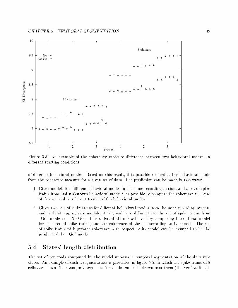
CHAPTER 5. TEMPORAL SEGMENTATION 496.5

7

7.5

8

8.5

9

9.5

10

1 2 3 1 2 3

KL

Div

ergen

ce

Trial #

15 clusters

8 clusters

GoNo Go

Figure 5.3: An example of the coherency measure di�erence between two behavioral modes, indi�erent starting conditions.of di�erent behavioral modes. Based on this result, it is possible to predict the behavioral modefrom the coherence measure for a given set of data. The prediction can be made in two ways:1. Given models for di�erent behavioral modes in the same recording session, and a set of spiketrains from and unknown behavioral mode, it is possible to compute the coherence measureof this set and to relate it to one of the behavioral modes.2. Given two sets of spike trains for di�erent behavioral modes from the same recording session,and without appropriate models, it is possible to di�erentiate the set of spike trains from\Go" mode vs. \No-Go". This di�erentiation is achieved by computing the optimal modelfor each set of spike trains, and the coherence of the set according to its model. The setof spike trains with greater coherence with respect to its model can be assumed to be theproduct of the \Go" mode.5.4 States' length distributionThe set of centroids computed by the model imposes a temporal segmentation of the data intostates. An example of such a segmentation is presented in �gure 5.5, in which the spike trains of 8cells are shown. The temporal segmentation of the model is drawn over them (the vertical lines).

CHAPTER 5. TEMPORAL SEGMENTATION 50

0

0.2

0.4

0.6

0.8

1

2 4 6 8 10 12 14 16 18 20

Accu

mo

late

tim

e s

eg

me

nt

Le

ng

ths

Time (ms*100)

’length_go’’length_nogo’

Figure 5.4: An example of length distribution among segmentation of di�erent behavioral mode.Consecutive basic time units (each consisting of 100 ms) belonging to the same state constitute atime segment. The indexes of these segments are shown above the spike trains, at the top of the�gure. These indexes will henceforth be called the labels of the segments.Figure 5.4 presents the accumulated distribution of segment lengths for both behavioral modesfrom one recording session. At each time point t, the percentage of segments whose length is smallerthan t is presented. For example, segments with a length of up to 1500ms account for 79.4% of allthe data in the \No-Go" mode, and for 70.8% of the data in the \Go" mode. It can be seen thatthe probability of �nding longer segments in the "Go" mode is higher than in the "No-Go" mode,which means that the segments of the \Go" mode are longer than those of the \No-Go" mode.This phenomenon is consistent over all the segments of length 1000 ms and above.This phenomenon was observed in 3 out of the 5 recording sessions, as seen in table 5.2. Thistable presents the percentage of segments with lengths up to 1500 ms, for both behavioral modesin all the recording sessions.

CHAPTER 5. TEMPORAL SEGMENTATION 510 2 1 0 2 1 0 1 0

T i m e

C e

l l

s

Figure 5.5: An example of a typical segmentation of spike trains of 8 cells.5.5 E�ect of full HMM implementationA full Hidden MarkovModel is the term used here to describe the insertion of transition probabilitiesbetween states into the previously computed models. The computation of the full Hidden MarkovModels of the data was done in two di�erent ways (Baum-Welch algorithm and segmental K-meansalgorithm) as described in Chapter 4 Section 4. The results of these algorithms included thetemporal segmentation of the spike train, and the likelihood of the data given the computed model.5.5.1 Di�erences between the Baum-Welch algorithm and the segmental K-meansThe results of the Baum-Welch algorithm and the segmental K-means were almost identical. Theywere identical in both result types, i.e. in the likelihood and the temporal segmentation. Table 5.3presents typical likelihood values of one recording session as computed according to the followingmethods:1. Clustering algorithm (K-means).

CHAPTER 5. TEMPORAL SEGMENTATION 52Session \Go" mode percentage \No-Go" mode percentagebl16 70.8 79.4bl25 82.4 87.4bl39 49.2 58.7cl77 76.3 84.1cl85 82.5 82.7Table 5.2: The percentage of segments with lengths up to 1500 ms, for both behavioral modes inall the recording sessions.2. The segmental K-means.3. The Baum-Welch algorithm.The likelihood values shown are the log likelihood per vector, i.e. N�1log(p�(x)), where N is thenumber of �ring rate vectors, � is the estimated model for the data, and x are the �ring ratevectors.Session K-means segmental K-means Baum-Welchbl16 -0.88 -0.85 -0.85bl25 -1.95 -1.90 -1.89bl29 -1.03 -1.01 -0.99bl39 -0.98 -0.97 -0.97cl77 -1.01 -1.00 -0.99cl85 -1.34 -1.33 -1.33Table 5.3: The likelihood values achieved in the di�erent training algorithms.These likelihood values show a sustained behavior, i.e. the changes between the di�erent com-putations is only minor compared with the likelihood values themselves. This behavior was seen inall the recording sessions. The computation of algorithms No. 2 and 3 was done on the same initialvalues reached in algorithm No. 1. Thus, it is possible to use the segmental K-means algorithminstead of the time consuming Baum-Welch algorithm, for this type of analysis.5.5.2 Changes in temporal segmentation due to a full HMMThe main e�ect of the HMM on the temporal segmentation was the smoothing of the segmentsequence, i.e. elimination of short segments and their absorption into longer segments. Smoothingis de�ned as the process of eliminating short, low-probability, state segments (usually 100-200 mslong) from the state sequence. This resulted from the insertion of transition probabilities into themodel. The probability of short segments is therefore very small, and most of them are removed.

CHAPTER 5. TEMPORAL SEGMENTATION 53Thus, the main determinant of the segment label is the multivariate Poisson probability. Thetransition probabilities govern only the elimination of short segments, and not the labeling ofsegments.An example of the di�erences between the clustering result and the full Hidden Markov Modelcan be seen in �gure 5.6. Figure 5.6a shows the spike trains of 8 cells. On each of the spike trains,the �ring rate is drawn. The temporal segmentation according to the Hidden Markov Model isdepicted above the arrow (but should be extrapolated to the entire dot-display). The labels ofstates according to this segmentation appear above the graph. The segmentation according toclustering is depicted below the arrow (and should also be extrapolated to the entire dot-display).The labels of states according to this segmentation appear below the graph. Figure 5.6b is parallelto �gure 5.6a, and presents the probabilities for being in each of the states depicted in �gure 5.6a ateach time point. The probability calculation was carried out based on the vector of �ring rates ateach time point. It can be seen that the temporal segmentation of the clustering is derived directlyfrom the probability graph (see �gure 5.6a below the arrow), whereas the segmentation of the fullHMM results only in the smoothing of this graph (see same �gure above the arrow).The e�ect of a smoothing process can be seen in the two temporal segmentations of data in�gure 5.6a. The state sequence in the clustering segmentation (see below the dot-display) is "1 5 14 1 5 2 4", whereas in the full HMM, the state sequence is just \1 5 4"(see above the dot-display).It can be seen that the �rst appearance of state No. 5, and the �rst appearance of state No. 4 areeliminated from the clustering segmentation, and both are replaced by state No. 1. This exchangeof states is the result of the fact that states No. 5 and No. 4 are short segments (100 ms longeach), with a low probability (as seen in the probability graph of �gure 5.6b). State No. 1, onthe other hand, has a higher probability, on average, in the whole region under discussion (statesegment No. 1 according to the HMM segmentation).It was found that this smoothing process is responsible for 96% of the di�erences betweenthe HMM segmentation and the clustering segmentation. Smoothing, therefore, constitutes thestrongest e�ect of the full HMM model. These �ndings were consistent over all the recordingsessions.5.6 E�ect of insertion of �ring rate cross-correlations into themodelThe insertion of the cross-correlation coe�cients into the HMM did not alter the temporal seg-mentation of the data. The vast majority of cross-correlation coe�cients computed were zero,indicating that no pair-wise cross-correlation exists between the �ring rate of di�erent cells in asingle cluster. Furthermore, in the rare instances when these coe�cients were not-zero, their valueswere very small, and did not e�ect the temporal segmentation of the data in any way.An example of a result of this calculation can be seen in �gure 5.7. Three covariance matricesof 7 cells are shown, indicating the correlation between the vectors in each of three di�erent states.The �ndings from these matrices are:1. Almost all of the non-diagonal elements in each matrix are zero.2. The largest absolute values that the elements in the covariance matrix reached are -0.20 and0.12.

CHAPTER 5. TEMPORAL SEGMENTATION 543. The covariance elements that hold non-zero values change their values in di�erent states, i.e.no signi�cant cross-correlation is indicated by these matrices.In each matrix, the highest covariance value was chosen (marked in the �gure), and the cross-correlation was computed between the �ring rates of these cells (using the iterative algorithmdescribed in Chapter 4 Section 5). In the example shown, the cross-correlation coe�cients for all3 matrices were identically zero. These values were reached after 3-4 iterations of the algorithm.These coe�cients did not change the temporal segmentation at all.5.7 Prediction of events based on state sequencesOur original hypothesis was that the sequences of states would be able to predict the events ofthe animal at the time of measurement. The results of the prediction test (described in Chapter4 Section 6) are presented in table 5.4. This table includes the following information for eachprediction trial:1. The recording session code.2. The number of sequence appearances in the data, for a speci�c sequence computed for thistrial.3. The number of times that the sequence successfully predicted the event under examination.4. The total number of appearance for that event in the recorded data.Session Sequence num Correct predictions Total Eventsbl16 243 21 281bl29 170 12 157bl29 123 10 78cl77 327 32 403cl77 411 28 403Table 5.4: Typical examples of prediction of events using states' sequences.This table shows that this hypothesis was not con�rmed unequivocally from the data presentedup to this point. That is, the simple sequences of states by themselves cannot give reasonableprediction of the events of the animal. However, some observations do seem to lend some supportto the hypothesis. Figure 5.8 illustrates this point. Figure 5.8a and 5.8b represent dot-displays ofthe same 8 cells, at two di�erent points of time during one recording session. In the two �gures,the line marked Start refers to the same external cue (in this case, beginning of trial of a "Go"mode). It can be seen that the state sequence following this Start is identical at the two points oftime. The sequence is "1 5 2".

CHAPTER 5. TEMPORAL SEGMENTATION 55This example and many other similar �ndings, suggest that a connection does exist betweensequences of states and external cues - but this connection had not yet been successfully captured.

CHAPTER 5. TEMPORAL SEGMENTATION 560

1

2

3

4

5

C l u s t e r P r o b a b i l t y

0

1

2

3

4

5

T i m e

P r o

b a

b i

l i t

y

1 5 1 4 1 5 2 4

1 5 4

T i m e

C e

l l

s

a.

b.

Figure 5.6: An example of two temporal segmentations of the same data (a.) and all their clusters'respective probabilities (b.) .

CHAPTER 5. TEMPORAL SEGMENTATION 571.0000 −0.0503 −0.0160 0.0302 0.0080 −0.0171 0.0095

−0.0503 1.0000 −0.0021 0.0088 −0.0978 −0.0085 0.0193

−0.0160 −0.0021 1.0000 0.0168 0.0051 0.0380 0.0066

0.0302 0.0088 0.0168 1.0000 −0.0377 0.0001 0.0353

0.0080 −0.0978 0.0051 −0.0377 1.0000 0.0019 −0.0092

−0.0171 −0.0085 0.0380 0.0001 0.0019 1.0000 −0.0009

0.0095 0.0193 0.0066 0.0353 −0.0092 −0.0009 1.0000

1.0000 0.1234 −0.1046 0.0277 0.0908 −0.0504 −0.0253

0.1234 1.0000 −0.0169 0.0128 0.1727 −0.0217 0.0546

−0.1046 −0.0169 1.0000 0.0244 0.0276 0.0335 0.0802

0.0277 0.0128 0.0244 1.0000 0.0309 −0.0254 0.0246

0.0908 0.1727 0.0276 0.0309 1.0000 −0.2059 0.0180

−0.0504 −0.0217 0.0335 −0.0254 −0.2059 1.0000 0.1494

−0.0253 0.0546 0.0802 0.0246 0.0180 0.1494 1.0000

1.0000 −0.0821 −0.0095 0.0025 −0.0252 −0.0081 −0.0046

−0.0821 1.0000 −0.0031 0.0052 −0.0370 −0.0048 0.0032

−0.0095 −0.0031 1.0000 −0.0205 0.0184 0.1118 0.0080

0.0025 0.0052 −0.0205 1.0000 −0.0097 −0.0385 0.0058

−0.0252 −0.0370 0.0184 −0.0097 1.0000 0.0062 −0.0153

−0.0081 −0.0048 0.1118 −0.0385 0.0062 1.0000 0.0153

−0.0046 0.0032 0.0080 0.0058 −0.0153 0.0153 1.0000

Cells

state 3

state 2

state 1

1 2 3 4 5 6 7Figure 5.7: An example of covariance matrices of 7 cells in 3 di�erent states.

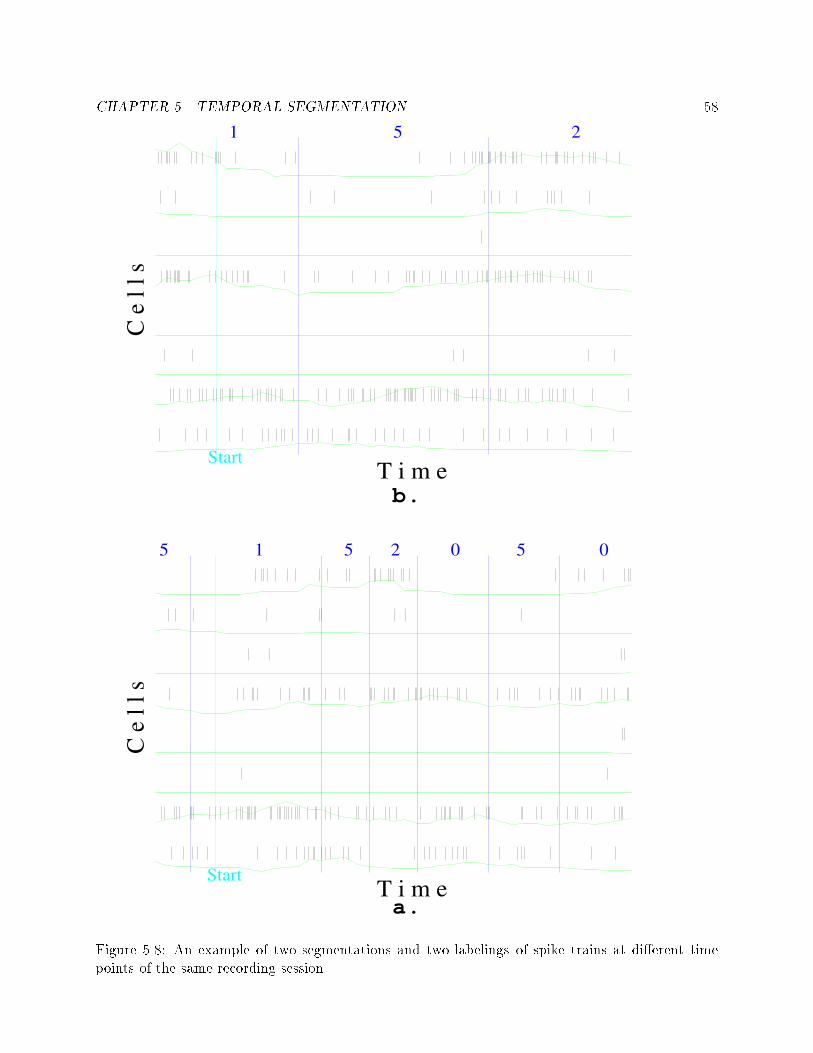
CHAPTER 5. TEMPORAL SEGMENTATION 581 5 2

StartT i m e

C e

l l

s

5 1 5 2 0 5 0

StartT i m e

C e

l l

s

a.

b.

Figure 5.8: An example of two segmentations and two labelings of spike trains at di�erent timepoints of the same recording session.

Chapter 6Temporal Cross Correlations indi�erent states6.1 Working hypothesesThe previous chapter dealt with cross-correlations between �ring rates of cells. In the presentchapter, the temporal cross-correlation of spike trains of cells will be discussed. The �ring ratecross-correlation was computed over a computation window of 500ms width, whereas the temporalcross-correlation is computed in lags of single ms. The goal of the test presented in this chapterwas to check the existence of di�erences between cross-correlation functions of this type in di�erentstates of the HMM, and thus, to try to connect the ideas underlying the cell-assembly hypothesiswith the HMM based model.A non- at temporal cross-correlation function of two cells may be the result of one of thefollowing possible situations:1. Direct interaction between the two cells, as a result of a strong synapse.2. Both cells are derived from a common input, which may be the hypothesized cell-assembly.In the second case the cross-correlation function is expected to change in di�erent states of orga-nization of the network - di�erent activations of cell-assemblies. These changes may occur in timeconstants of tens to hundreds of ms.6.2 Cells with su�cient dataThe computation of the temporal cross-correlation was done as described in Chapter 4 Section 8.This �rst stage of computation consisted of choosing the states whose length was above a certainthreshold. In this test the threshold used was 1000 ms. As a result of this �ltering, only part ofthe data could be used for further analysis. The percentage of data used is shown in table 6.1. Theinformation included in the table is as follows:1. The recording session code.2. The total length of data in the recording session (in ms).59

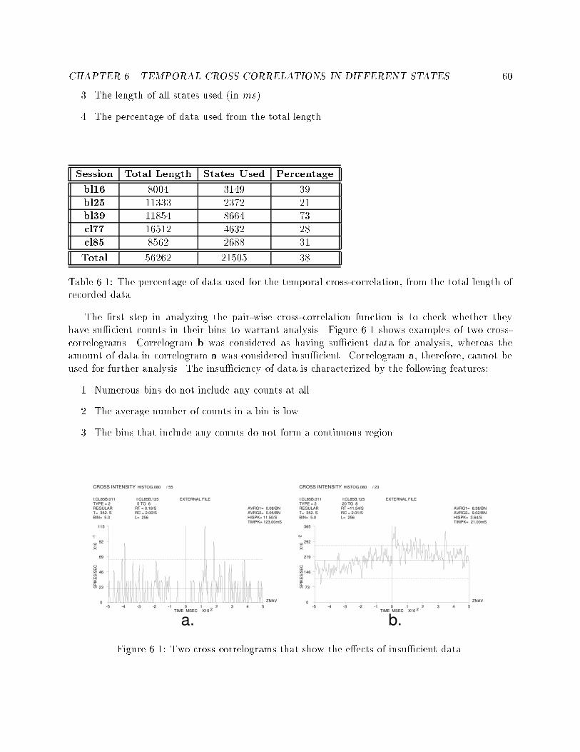
CHAPTER 6. TEMPORAL CROSS CORRELATIONS IN DIFFERENT STATES 603. The length of all states used (in ms).4. The percentage of data used from the total length.Session Total Length States Used Percentagebl16 8004 3149 39bl25 11333 2372 21bl39 11854 8664 73cl77 16512 4632 28cl85 8562 2688 31Total 56262 21505 38Table 6.1: The percentage of data used for the temporal cross-correlation, from the total length ofrecorded data.The �rst step in analyzing the pair-wise cross-correlation function is to check whether theyhave su�cient counts in their bins to warrant analysis. Figure 6.1 shows examples of two cross-correlograms. Correlogram b was considered as having su�cient data for analysis, whereas theamount of data in correlogram a was considered insu�cient. Correlogram a, therefore, cannot beused for further analysis. The insu�ciency of data is characterized by the following features:1. Numerous bins do not include any counts at all.2. The average number of counts in a bin is low.3. The bins that include any counts do not form a continuous region.I:CL85B.011 I:CL85B.125 EXTERNAL FILE TYPE = 2 REGULAR T= 352. S BIN= 5.0

5 TO 6 RT = 0.18/S RC = 2.00/S L= 256

AVRG1= 0.08/BN AVRG2= 0.05/BN HISPK= 11.50/S TIMPK= 123.00mS

-5 -4 -3 -2 -1 0 1 2 3 4 5 TIME MSEC X10 2

0

23

46

69

92

115

SP

IKE

S/S

EC

X

10

-1

CROSS INTENSITY HISTOG.080 / 55

ZNAV

I:CL85B.011 I:CL85B.125 EXTERNAL FILE TYPE = 2 REGULAR T= 352. S BIN= 5.0

20 TO 8 RT =11.54/S RC = 2.01/S L= 256

AVRG1= 6.38/BN AVRG2= 9.02/BN HISPK= 3.64/S TIMPK= 21.00mS

-5 -4 -3 -2 -1 0 1 2 3 4 5 TIME MSEC X10 2

0

73

146

219

292

365

SP

IKE

S/S

EC

X

10

-2

CROSS INTENSITY HISTOG.080 / 23

ZNAV

a. b.Figure 6.1: Two cross correlograms that show the e�ects of insu�cient data.

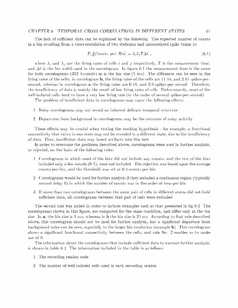
CHAPTER 6. TEMPORAL CROSS CORRELATIONS IN DIFFERENT STATES 61The lack of su�cient data can be explained by the following. The expected number of countsin a bin resulting from a cross-correlation of two stationar and uncorrelated spike trains is:Eij[Counts per Bin] = �i�jT�t ; (6:1)where �i and �j are the �ring rates of cells i and j respectively, T is the measurement time,and �t is the bin width used in the correlogram. In �gure 6.1 the measurement time is the samefor both correlograms (352 Seconds) as is the bin size (5 ms). The di�erence can be seen in the�ring rates of the cells: in correlogram b, the �ring rates of the cells are 11.54, and 2.01 spikes-per-second, whereas in correlogram a the �ring rates are 0.18, and 2.0 spikes-per-second. Therefore,the insu�ciency of data is mainly the result of low �ring rates of cells. Unfortunately, most of thewell-isolated cells tend to have a very low �ring rate (in the order of several spikes-per-second).The problem of insu�cient data in correlograms may cause the following e�ects:1. Noisy correlograms may not reveal an inherent delicate temporal structure.2. Departures from background in correlograms may be the outcome of noisy activity.These e�ects may be crucial when testing the working hypothesis - for example, a functionalconnectivity that exists in one state may not be revealed in a di�erent state, due to the insu�ciencyof data. Thus, insu�cient data may insert artifacts into this test.In order to overcome the problems described above, correlograms were used in further analysis,or rejected, on the basis of the following rules:1. Correlograms in which most of the bins did not include any counts, and the rest of the binsincluded only a few counts (0-5), were not included. The rejection was based upon the averagecounts-per-bin, and the threshold was set at 0.2 counts-per-bin.2. Correlograms would be used for further analysis if they included a continuous region (typicallyaround delay 0) in which the number of counts was in the order of tens-per-bin.3. If more than two correlograms between the same pair of cells in di�erent states did not holdsu�cient data, all correlograms between that pair of cells were excluded.The second rule was added in order to include examples such as that presented in �g 6.2. Thecorrelograms shown in this �gure, are computed for the same condition, and di�er only in the binsize. In a, the bin size is 5 ms, whereas in b the bin size is 25 ms. According to �rst rule describedabove, this correlogram should not be used for further analysis, but a signi�cant departure frombackground noise can be seen, especially in the larger bin resolution (example b). This correlogramshows a signi�cant functional connectivity between the cells, and rule No. 2 enables us to makeuse of it.The information about the correlograms that include su�cient data to warrant further analysis,is shown in table 6.2. The information included in the table is as follows:1. The recording session code.2. The number of well-isolated cells used in each recording session.

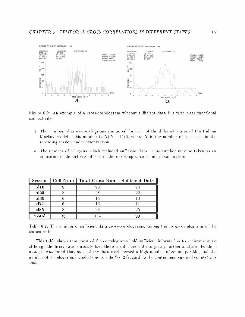
CHAPTER 6. TEMPORAL CROSS CORRELATIONS IN DIFFERENT STATES 62I:CL85B.009 I:CL85B.125 EXTERNAL FILE TYPE = 2 REGULAR T= 363. S BIN= 25.0

8 TO 10 RT = 1.06/S RC = 0.27/S L= 247

AVRG1= 0.15/BN AVRG2= 0.06/BN HISPK= 1.56/S TIMPK= 1.00mS

-5 -4 -3 -2 -1 0 1 2 3 4 5 TIME MSEC X10 2

0

32

64

96

128

160

SP

IKE

S/S

EC

X

10

-2

CROSS INTENSITY HISTOG.081 / 83

ZNAV

I:CL85B.009 I:CL85B.125 EXTERNAL FILE TYPE = 2 REGULAR T= 363. S BIN= 5.0

8 TO 10 RT = 1.06/S RC = 0.27/S L= 247

AVRG1= 0.15/BN AVRG2= 0.06/BN HISPK= 2.53/S TIMPK= -66.00mS

-5 -4 -3 -2 -1 0 1 2 3 4 5 TIME MSEC X10 2

0

51

102

153

204

255

SP

IKE

S/S

EC

X

10

-2

CROSS INTENSITY HISTOG.081 / 83

ZNAV

a. b.Figure 6.2: An example of a cross-correlogram without su�cient data but with clear functionalconnectivity3. The number of cross-correlograms computed for each of the di�erent states of the HiddenMarkov Model. This number is N(N � 1)=2, where N is the number of cells used in therecording session under examination.4. The number of cell-pairs which included su�cient data. This number may be taken as anindication of the activity of cells in the recording session under examination.Session Cell Num Total Cross Num Su�cient Databl16 8 28 28bl25 8 28 22bl39 6 15 13cl77 6 15 11cl85 8 28 25Total 36 114 99Table 6.2: The number of su�cient data cross-correlograms, among the cross-correlograms of thechosen cells.This table shows that most of the correlograms hold su�cient information to achieve results:although the �ring rate is usually low, there is su�cient data to justify further analysis. Further-more, it was found that most of the data used showed a high number of counts-per-bin, and thenumber of correlograms included due to rule No. 2 (regarding the continuous region of counts) wassmall.

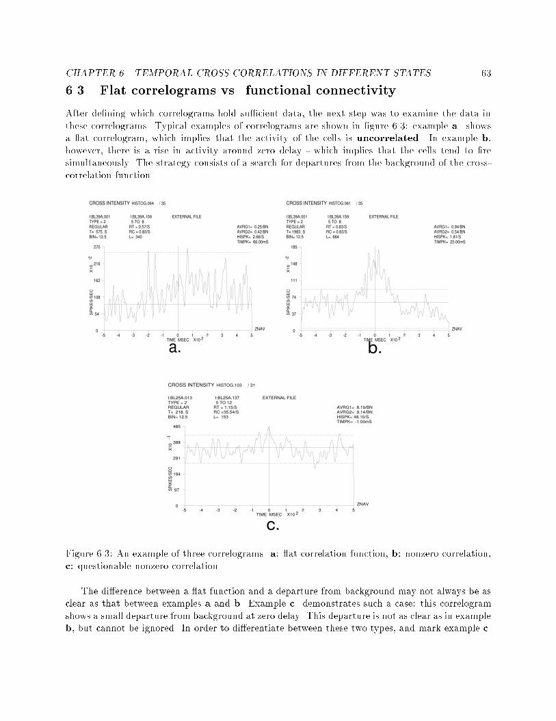
CHAPTER 6. TEMPORAL CROSS CORRELATIONS IN DIFFERENT STATES 636.3 Flat correlograms vs. functional connectivityAfter de�ning which correlograms hold su�cient data, the next step was to examine the data inthese correlograms. Typical examples of correlograms are shown in �gure 6.3: example a. showsa at correlogram, which implies that the activity of the cells is uncorrelated. In example b,however, there is a rise in activity around zero delay - which implies that the cells tend to �resimultaneously. The strategy consists of a search for departures from the background of the cross-correlation function.I:BL39A.001 I:BL39A.159 EXTERNAL FILE TYPE = 2 REGULAR T= 575. S BIN= 12.5

5 TO 8 RT = 0.57/S RC = 0.83/S L= 340

AVRG1= 0.25/BN AVRG2= 0.42/BN HISPK= 2.66/S TIMPK= 66.00mS

-5 -4 -3 -2 -1 0 1 2 3 4 5 TIME MSEC X10 2

0

54

108

162

216

270

SP

IKE

S/S

EC

X

10

-2

CROSS INTENSITY HISTOG.064 / 35

ZNAV

I:BL39A.001 I:BL39A.159 EXTERNAL FILE TYPE = 2 REGULAR T= 1983. S BIN= 12.5

5 TO 8 RT = 0.83/S RC = 0.63/S L= 684

AVRG1= 0.94/BN AVRG2= 0.54/BN HISPK= 1.81/S TIMPK= 25.00mS

-5 -4 -3 -2 -1 0 1 2 3 4 5 TIME MSEC X10 2

0

37

74

111

148

185

SP

IKE

S/S

EC

X

10

-2

CROSS INTENSITY HISTOG.061 / 35

ZNAV

a. b.

I:BL25A.013 I:BL25A.137 EXTERNAL FILE TYPE = 2 REGULAR T= 218. S BIN= 12.5

5 TO 12 RT = 1.15/S RC =35.54/S L= 153

AVRG1= 8.19/BN AVRG2= 9.14/BN HISPK= 48.10/S TIMPK= -1.00mS

-5 -4 -3 -2 -1 0 1 2 3 4 5 TIME MSEC X10 2

0

97

194

291

388

485

SP

IKE

S/S

EC

X

10

-1

CROSS INTENSITY HISTOG.103 / 31

ZNAV

c.Figure 6.3: An example of three correlograms. a: at correlation function, b: nonzero correlation,c: questionable nonzero correlationThe di�erence between a at function and a departure from background may not always be asclear as that between examples a and b. Example c. demonstrates such a case: this correlogramshows a small departure from background at zero delay. This departure is not as clear as in exampleb, but cannot be ignored. In order to di�erentiate between these two types, and mark example c.

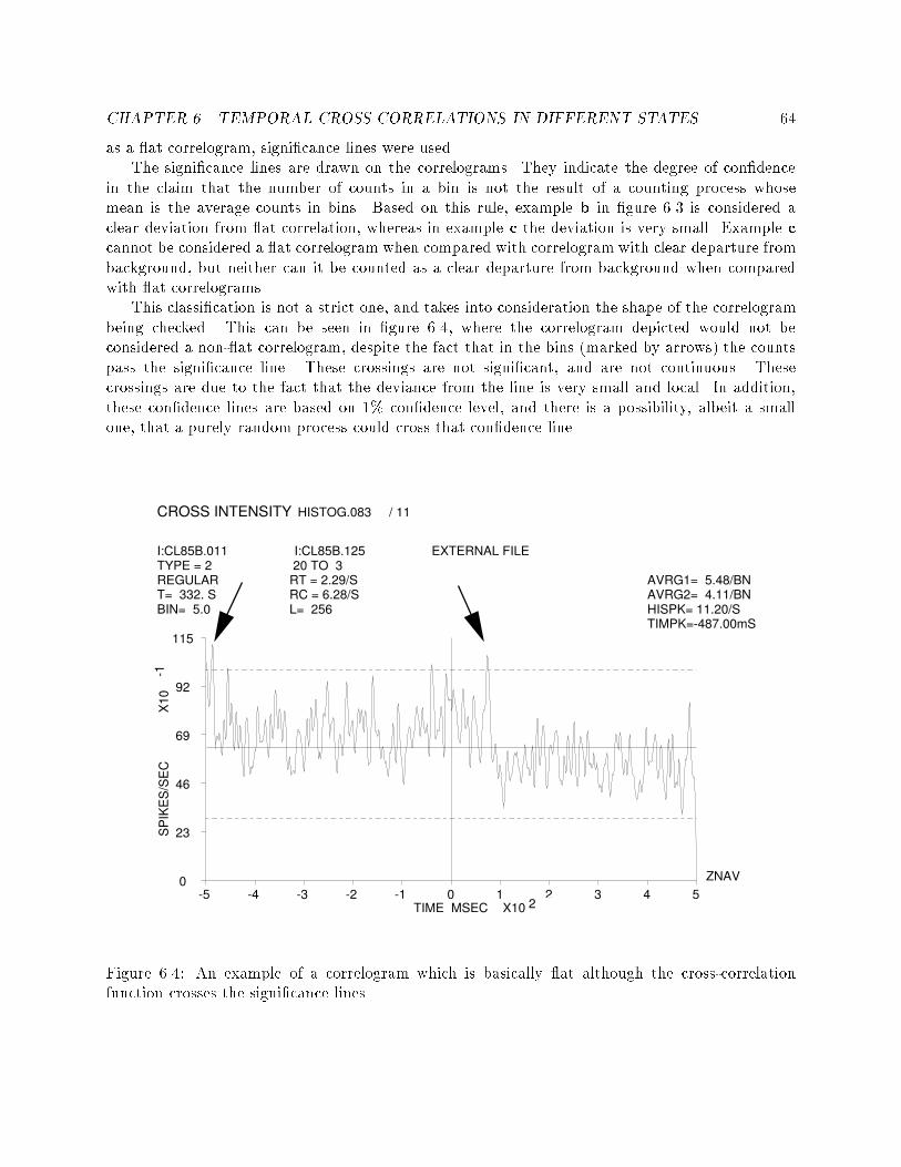
CHAPTER 6. TEMPORAL CROSS CORRELATIONS IN DIFFERENT STATES 64as a at correlogram, signi�cance lines were used.The signi�cance lines are drawn on the correlograms. They indicate the degree of con�dencein the claim that the number of counts in a bin is not the result of a counting process whosemean is the average counts in bins. Based on this rule, example b in �gure 6.3 is considered aclear deviation from at correlation, whereas in example c the deviation is very small. Example ccannot be considered a at correlogram when compared with correlogram with clear departure frombackground, but neither can it be counted as a clear departure from background when comparedwith at correlograms.This classi�cation is not a strict one, and takes into consideration the shape of the correlogrambeing checked. This can be seen in �gure 6.4, where the correlogram depicted would not beconsidered a non- at correlogram, despite the fact that in the bins (marked by arrows) the countspass the signi�cance line. These crossings are not signi�cant, and are not continuous. Thesecrossings are due to the fact that the deviance from the line is very small and local. In addition,these con�dence lines are based on 1% con�dence level, and there is a possibility, albeit a smallone, that a purely random process could cross that con�dence line.I:CL85B.011 I:CL85B.125 EXTERNAL FILE TYPE = 2 REGULAR T= 332. S BIN= 5.0

20 TO 3 RT = 2.29/S RC = 6.28/S L= 256

AVRG1= 5.48/BN AVRG2= 4.11/BN HISPK= 11.20/S TIMPK=-487.00mS

-5 -4 -3 -2 -1 0 1 2 3 4 5 TIME MSEC X10 2

0

23

46

69

92

115

SP

IKE

S/S

EC

X

10

-1

CROSS INTENSITY HISTOG.083 / 11

ZNAV Figure 6.4: An example of a correlogram which is basically at although the cross-correlationfunction crosses the signi�cance lines.

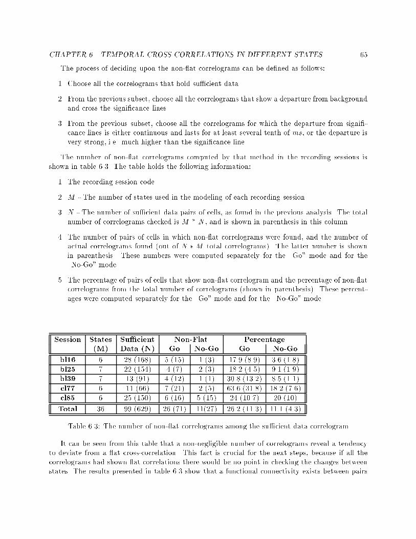
CHAPTER 6. TEMPORAL CROSS CORRELATIONS IN DIFFERENT STATES 65The process of deciding upon the non- at correlograms can be de�ned as follows:1. Choose all the correlograms that hold su�cient data.2. From the previous subset, choose all the correlograms that show a departure from backgroundand cross the signi�cance lines.3. From the previous subset, choose all the correlograms for which the departure from signi�-cance lines is either continuous and lasts for at least several tenth of ms, or the departure isvery strong, i.e. much higher than the signi�cance line.The number of non- at correlograms computed by that method in the recording sessions isshown in table 6.3. The table holds the following information:1. The recording session code.2. M - The number of states used in the modeling of each recording session3. N - The number of su�cient data pairs of cells, as found in the previous analysis. The totalnumber of correlograms checked is M * N , and is shown in parenthesis in this column.4. The number of pairs of cells in which non- at correlograms were found, and the number ofactual correlograms found (out of N �M total correlograms). The latter number is shownin parenthesis. These numbers were computed separately for the \Go" mode and for the\No-Go" mode.5. The percentage of pairs of cells that show non- at correlogram and the percentage of non- atcorrelograms from the total number of correlograms (shown in parenthesis). These percent-ages were computed separately for the \Go" mode and for the \No-Go" mode.Session States Su�cient Non-Flat Percentage(M) Data (N) Go No-Go Go No-Gobl16 6 28 (168) 5 (15) 1 (3) 17.9 (8.9) 3.6 (1.8)bl25 7 22 (154) 4 (7) 2 (3) 18.2 (4.5) 9.1 (1.9)bl39 7 13 (91) 4 (12) 1 (1) 30.8 (13.2) 8.5 (1.1)cl77 6 11 (66) 7 (21) 2 (5) 63.6 (31.8) 18.2 (7.6)cl85 6 25 (150) 6 (16) 5 (15) 24 (10.7) 20 (10)Total 36 99 (629) 26 (71) 11(27) 26.2 (11.3) 11.1 (4.3)Table 6.3: The number of non- at correlograms among the su�cient data correlogramIt can be seen from this table that a non-negligible number of correlograms reveal a tendencyto deviate from a at cross-correlation. This fact is crucial for the next steps, because if all thecorrelograms had shown at correlations there would be no point in checking the changes betweenstates. The results presented in table 6.3 show that a functional connectivity exists between pairs

CHAPTER 6. TEMPORAL CROSS CORRELATIONS IN DIFFERENT STATES 66of cells in speci�c states of the model. This result may be due to the modeling of the data, or itmay be the result of a prominent functional connectivity that exists throughout the whole recordingsession.This table also shows that the percentage of non- at correlograms is much higher in the \Go"mode than in the \No-Go" mode. In the \Go" mode 11.3% of the correlograms were non- at,whereas in the \No-Go" mode only 4.5% were non- at. This phenomenon is also seen in thepercentage of pairs of cells that show any correlation. In the \Go" mode they constitute 26.2%,whereas in the \No-Go" mode they constitute only 11.1%.6.4 Types of functional connectivityThe types of departures from background of the cross-correlation function that were found in thisanalysis, can be seen in �gure 6.5. There were 4 types:A. Narrow peak con�ned to one side of the origin, in this example to the positive side.B. Narrow peak in the correlogram - straddling the zero delay.C. Narrow trough con�ned to one side of the origin, in this example to the negative side.D. Wide peak straddling the zero delay in the correlogram.The terms wide and narrow refer to the departure time. By wide we mean a peak or a troughthat lasts more than 200 ms and by narrow - that the time constants involved are 10-100 ms.Types B and D are usually referred to as shared or common input.After computing all the non- at correlograms, they were classi�ed according to these four types.Table 6.4 shows this classi�cation:Session Type A Type B Type C Type D Totalbl16 4 7 7 18bl25 2 8 10bl39 2 1 10 13cl77 2 16 3 5 26cl85 3 13 15 31Total 11 39 3 45 98Table 6.4: The classi�cation of non- at correlograms into four types of functional connectivityThis table shows that 46% of the non- at correlograms showed wide peaks, and 40% showednarrow peaks. Thus these two types constitute 86% of the total number of non- at correlograms.It should be noted that no troughs straddling zero delays were found in this experiment.

CHAPTER 6. TEMPORAL CROSS CORRELATIONS IN DIFFERENT STATES 67I:BL16A.005 I:BL16A.099 EXTERNAL FILE TYPE = 2 REGULAR T= 343. S BIN= 10.0

1 TO 4 RT = 2.97/S RC = 8.89/S L= 227

AVRG1= 8.91/BN AVRG2= 7.98/BN HISPK= 12.55/S TIMPK= 29.00mS

-5 -4 -3 -2 -1 0 1 2 3 4 5 TIME MSEC X10 2

0

26

52

78

104

130

SP

IKE

S/S

EC

X

10

-1

CROSS INTENSITY HISTOG.052 / 19

ZNAV

I:CL77B.002 I:CL77B.253 EXTERNAL FILE TYPE = 2 REGULAR T= 862. S BIN= 10.0

13 TO 14 RT = 2.33/S RC = 0.60/S L= 569

AVRG1= 1.23/BN AVRG2= 0.58/BN HISPK= 3.36/S TIMPK= 0.00mS

-5 -4 -3 -2 -1 0 1 2 3 4 5 TIME MSEC X10 2

0

68

136

204

272

340

SP

IKE

S/S

EC

X

10

-2

CROSS INTENSITY HISTOG.121 / 67

ZNAV

I:CL77B.036 I:CL77B.251 EXTERNAL FILE TYPE = 2 REGULAR T= 66. S BIN= 10.0

8 TO 14 RT = 7.58/S RC =12.29/S L= 48

AVRG1= 6.80/BN AVRG2= 6.16/BN HISPK= 17.23/S TIMPK=-499.00mS

-5 -4 -3 -2 -1 0 1 2 3 4 5 TIME MSEC X10 2

0

35

70

105

140

175

SP

IKE

S/S

EC

X

10

-1

CROSS INTENSITY HISTOG.123 / 55

ZNAV

I:BL39A.003 I:BL39A.159 EXTERNAL FILE TYPE = 2 REGULAR T= 713. S BIN= 10.0

5 TO 8 RT = 1.05/S RC = 0.70/S L= 374

AVRG1= 0.44/BN AVRG2= 0.32/BN HISPK= 3.01/S TIMPK= -67.00mS

-5 -4 -3 -2 -1 0 1 2 3 4 5 TIME MSEC X10 2

0

61

122

183

244

305

SP

IKE

S/S

EC

X

10

-2

CROSS INTENSITY HISTOG.062 / 35

ZNAV

a. b.

c. d.

Figure 6.5: An example of di�erent types of functional connectivity6.5 Modi�cation of pair-wise cross-correlation functions betweenstatesThe Modi�cation of Pair-wise Cross-correlation function between States (MPCS) is de�ned as allpairs of cells that have di�erent types of functional connectivity in di�erent states of the model,i.e. in one of the states one type of functional connectivity is observed, whereas in other states adi�erent functional connectivity is seen. When computing all the MPCS, it was possible to use the at type, i.e. an MPCS event would be counted if in one of the states a type C cross-correlationwas observed, and in the other a at correlation was seen. In any case of doubt regarding theexistence of a functional connectivity, the criterion was as strict as possible. The MPCS would notbe counted if either:� It was not clear that a functional connectivity existed.

CHAPTER 6. TEMPORAL CROSS CORRELATIONS IN DIFFERENT STATES 68� It was not absolutely clear that the correlogram was at.A typical example of such a situation is shown in �gure 6.6. In this example, the number ofstates of the HMM is 7, so correlograms numbered from 0 to 6 of the same pair of cells (No. 5and No. 8), are depicted. Each of these correlograms was computed for the spike trains of thematching state. In the correlogram of state No. 1, a clear, non- at, cross-correlation function existsbetween the pair of cells, whereas in the correlogram of state No. 6 the correlogram is of the attype. The cross-correlation function in state No. 1 is of a common input type, i.e. the rise of thecross-correlation function above the signi�cance line occurs on both sides of zero time. The sizeof this rise is in the order of several hundreds of ms. In the correlograms of states 0, 2 and 3, asimilar, common input phenomenon is shown. In state 3, however, the departure from backgroundand crossing of the signi�cance line are much weaker compared with states 0-2. On the other hand,in the correlograms of states 4, 5 and 6 no such departure is seen.I:BL39A.003 I:BL39A.159 EXTERNAL FILE TYPE = 2 REGULAR T= 219. S BIN= 10.0

5 TO 8 RT = 7.02/S RC = 1.15/S L= 121

AVRG1= 1.32/BN AVRG2= 2.26/BN HISPK= 2.66/S TIMPK= 31.00mS

-5 -4 -3 -2 -1 0 1 2 3 4 5 TIME MSEC X10 2

0

54

108

162

216

270

SP

IK

ES

/S

EC

X

10

-2

CROSS INTENSITY HISTOG.060 / 35

ZNAV

I:BL39A.001 I:BL39A.159 EXTERNAL FILE TYPE = 2 REGULAR T= 1983. S BIN= 10.0

5 TO 8 RT = 0.83/S RC = 0.63/S L= 684

AVRG1= 0.94/BN AVRG2= 0.54/BN HISPK= 1.95/S TIMPK= 25.00mS

-5 -4 -3 -2 -1 0 1 2 3 4 5 TIME MSEC X10 2

0

39

78

117

156

195

SP

IK

ES

/S

EC

X

10

-2

CROSS INTENSITY HISTOG.061 / 35

ZNAV

I:BL39A.003 I:BL39A.159 EXTERNAL FILE TYPE = 2 REGULAR T= 713. S BIN= 10.0

5 TO 8 RT = 1.05/S RC = 0.70/S L= 374

AVRG1= 0.44/BN AVRG2= 0.32/BN HISPK= 3.01/S TIMPK= -67.00mS

-5 -4 -3 -2 -1 0 1 2 3 4 5 TIME MSEC X10 2

0

61

122

183

244

305

SP

IK

ES

/S

EC

X

10

-2

CROSS INTENSITY HISTOG.062 / 35

ZNAV

I:BL39A.001 I:BL39A.159 EXTERNAL FILE TYPE = 2 REGULAR T= 635. S BIN= 10.0

5 TO 8 RT = 4.44/S RC = 0.64/S L= 358

AVRG1= 1.51/BN AVRG2= 1.75/BN HISPK= 1.24/S TIMPK= -13.00mS

-5 -4 -3 -2 -1 0 1 2 3 4 5 TIME MSEC X10 2

0

25

50

75

100

125

SP

IK

ES

/S

EC

X

10

-2

CROSS INTENSITY HISTOG.063 / 35

ZNAV

I:BL39A.001 I:BL39A.159 EXTERNAL FILE TYPE = 2 REGULAR T= 575. S BIN= 10.0

5 TO 8 RT = 0.57/S RC = 0.83/S L= 340

AVRG1= 0.25/BN AVRG2= 0.42/BN HISPK= 2.91/S TIMPK=-200.00mS

-5 -4 -3 -2 -1 0 1 2 3 4 5 TIME MSEC X10 2

0

59

118

177

236

295

SP

IK

ES

/S

EC

X

10

-2

CROSS INTENSITY HISTOG.064 / 35

ZNAV

I:BL39A.001 I:BL39A.151 EXTERNAL FILE TYPE = 2 REGULAR T= 309. S BIN= 10.0

5 TO 8 RT =14.28/S RC = 1.83/S L= 180

AVRG1= 8.33/BN AVRG2= 13.02/BN HISPK= 3.37/S TIMPK= 478.00mS

-5 -4 -3 -2 -1 0 1 2 3 4 5 TIME MSEC X10 2

0

68

136

204

272

340

SP

IK

ES

/S

EC

X

10

-2

CROSS INTENSITY HISTOG.065 / 35

ZNAV

I:BL39A.001 I:BL39A.151 EXTERNAL FILE TYPE = 2 REGULAR T= 209. S BIN= 10.0

5 TO 8 RT = 2.84/S RC = 3.75/S L= 117

AVRG1= 2.70/BN AVRG2= 2.79/BN HISPK= 6.49/S TIMPK= 300.00mS

-5 -4 -3 -2 -1 0 1 2 3 4 5 TIME MSEC X10 2

0

13

26

39

52

65

SP

IK

ES

/S

EC

X

10

-1

CROSS INTENSITY HISTOG.066 / 35

ZNAV

0 1 2 3

4 5 6

Figure 6.6: All the correlograms of a pair of cells in di�erent states.Some other phenomena should be noted in this example:1. The �ring rate of the cells is very low (less than a spike-per-second for most of the states),but still, a very persuasive correlation function can be seen. For example the �ring rates ofcell No. 8 in states No. 0-4 are 1.15, 0.63, 0.7, 0.64, 0.83 respectively. The �ring rates of cellNo. 5 in states No. 1,2,4 are 0.83, 1.05, 0.57 respectively.

CHAPTER 6. TEMPORAL CROSS CORRELATIONS IN DIFFERENT STATES 692. Correlation shapes may change between two states even when almost no changes exists inthe �ring rate of the pair of cells. For example, in state No. 1, cell No. 5 �res at a rate of0.83 spikes per second, whereas in state No. 4 the average �ring rate is 0.57. For cell No.8, the �ring rates are 0.63 spikes per second and 0.83 spikes per second respectively. Therelationship between MPCS and the �ring rate in di�erent states will be discussed later.3. A rise is seen on the positive end of the correlogram of state No. 5. A possible explanationof this rise is the tendency of cells to intensify their �ring rate towards the end of the state.Such an explanation, however, goes beyond the scope of the current research.In table 6.5 the results of this stage of analysis are shown. The table presents the followinginformation:1. The recording session.2. The total number of pairs of cells with su�cient data.3. The number of MPCS occurrences in the \Go" mode.4. The number of MPCS occurrences in the \No-Go" mode.It can be seen that a non-negligible number of cell pairs show occurrences of MPCS, and that thispercentage is much higher in the \Go" mode compared to the \No-Go" mode.Session name Su�cient Data \Go" mode \No-Go" modebl16 28 5 1bl25 22 4 2bl39 13 4 1cl77 11 6 2cl85 25 6 4Total 99 25 10Table 6.5: The number of MPCS occurrences - classi�ed into \Go" trials and \No-Go" trials, andcompared with the total number of su�cient data cell-pairs.6.6 Contamination of spike train as a cause of MPCSA possible artifact regarding the occurrences of MPCS may be due to contamination of spike trainsfrom di�erent recorded cells. This contamination may result in a cross-correlation functions whichis a mixture of several correlation functions, whose relative weight change over time. These errorsmay result an inaccurate MPCS. This contamination may be the result of two factors:1. Insu�cient isolation between cells: the recorded spike trains of the cells consisted of theaction potentials of two or more neurons. This insu�cient isolation was discussed in detailin Chapter 3 Section 4.

CHAPTER 6. TEMPORAL CROSS CORRELATIONS IN DIFFERENT STATES 702. Cells recorded from the same electrode: the two cells were recorded from the same electrode,thus the probability of the cells contaminating each other is higher then usual.Each of these factors was checked, by going over all the MPCS occurrences found and checkingthe supposed in uence of the factors compared with the MPCS occurrences found without theirpresence.6.6.1 Insu�cient isolation between cellsTable 6.6 shows the isolation quality of cells participating in all of the MPCS occurrences (both\Go" mode and \No-Go" mode). This isolation quality is the score the cells were given during therecording session (Chapter 3 Section 4), and is divided into 3 classes:1. Both cells were well-isolated neurons, i.e. both of them are of type A or B.2. One of the cells is a well-isolated neuron, whereas the other may be a mixture of two neurons.In score terms, this means that one of the cells is of type B and above, and the other is oftype C and above.3. Both of the cells are mixtures of two neurons, i.e. both of them are of type C and below.Session B - B pairs B - C pairs C - C pairsbl16 1 4 1bl25 0 4 2bl39 4 1 0cl77 4 4 0cl85 7 3 0Total 16 16 3Table 6.6: Classi�cation of MPCS occurrences for each recording session into three groups: A or Btypes, B or C types, and all the other types.Table 6.6 shows that 45% of the MPCS occurrences (16 out of 35) are from well-isolated neurons,91% of them (32 out of 35) are from at least one isolated neuron, and only 9% (3 out of 35) arefrom cells that are both mixtures of two neurons. Thus the vast majority of MPCS occurrenceswere from pairs of cells which are well-isolated cells, and the probability of contamination is verysmall.6.6.2 Cells recorded from the same electrodeAs explained previously (Chapter 3 Section 4), cells recorded from the same electrode have a higherrisk of cross-contamination, thus creating artifacts in their cross-correlation function. Therefore,

CHAPTER 6. TEMPORAL CROSS CORRELATIONS IN DIFFERENT STATES 71the following test was conducted: the number of MPCS occurrences from the same electrode wascompared with the number of MPCS occurrences from di�erent electrodes. This check is presentedin table 6.7 and includes the following information:1. The recording session code.2. The number of MPCS occurrences that were computed for cells from:(a) The same electrode in the \Go" mode.(b) Di�erent electrodes in the \Go" mode.(c) The same electrode in the \No-Go" mode.(d) Di�erent electrodes in the \No-Go" mode.3. The total number of pairs that were recorded from the same electrode. This number is thesame for \Go" and \No-Go" modes.4. The total number of pairs that were recorded from di�erent electrodes.Session Go:same Go:di� No-Go:same No-Go:di� All:same All:di�bl16 1 4 0 1 2 26bl25 1 3 0 2 3 25bl39 1 3 0 1 2 13cl77 1 5 0 2 1 14cl85 1 5 0 4 2 26Total 5 20 0 10 10 104Table 6.7: The number of MPCS occurrences from the same electrode and from di�erent electrodes,in the 2 behavioral modes.This table shows clearly that most of the MPCS were the result of cells recorded from di�erentelectrodes - 80% in the \Go"mode (20 out of 25) and 100% in the \No-Go" mode (10 out of 10). Thetotal percentage of MPCS recorded from di�erent electrodes is 86% (30 out of 35). Furthermore,the total number of pairs of cells recorded from di�erent electrodes used in this experiment was 91%.(104 out of 114). Thus, the percentage of MPCS occurrences recorded from di�erent electrodes isvery similar to that of the percentage of total number of cell pairs recorded from di�erent electrodes.This result enables us to disregard the possibility that the MPCS occurrences were an artifact ofcells recorded from the same electrode.6.7 Types of MPCSFigure 6.3 shows one type of MPCS: the transition from a at correlogram a to a common inputcorrelogram b. There are many types of such MPCS, each with its biological explanation. The

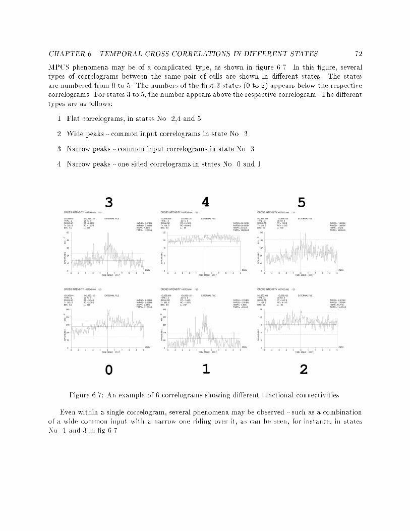
CHAPTER 6. TEMPORAL CROSS CORRELATIONS IN DIFFERENT STATES 72MPCS phenomena may be of a complicated type, as shown in �gure 6.7. In this �gure, severaltypes of correlograms between the same pair of cells are shown in di�erent states. The statesare numbered from 0 to 5. The numbers of the �rst 3 states (0 to 2) appears below the respectivecorrelograms. For states 3 to 5, the number appears above the respective correlogram. The di�erenttypes are as follows:1. Flat correlograms, in states No. 2,4 and 52. Wide peaks - common input correlograms in state No. 33. Narrow peaks - common input correlograms in state No. 3.4. Narrow peaks - one sided correlograms in states No. 0 and 1.I:CL85B.011 I:CL85B.125 EXTERNAL FILE TYPE = 2 REGULAR T= 352. S BIN= 5.0

20 TO 8 RT =11.54/S RC = 2.01/S L= 256

AVRG1= 6.38/BN AVRG2= 9.02/BN HISPK= 3.64/S TIMPK= 21.00mS

-5 -4 -3 -2 -1 0 1 2 3 4 5 TIME MSEC X10 2

0

73

146

219

292

365

SP

IKE

S/S

EC

X

10

-2

CROSS INTENSITY HISTOG.080 / 23

ZNAV

I:CL85B.009 I:CL85B.125 EXTERNAL FILE TYPE = 2 REGULAR T= 363. S BIN= 5.0

20 TO 8 RT = 1.64/S RC = 1.06/S L= 247

AVRG1= 0.20/BN AVRG2= 0.35/BN HISPK= 4.40/S TIMPK= -4.00mS

-5 -4 -3 -2 -1 0 1 2 3 4 5 TIME MSEC X10 2

0

88

176

264

352

440

SP

IKE

S/S

EC

X

10

-2

CROSS INTENSITY HISTOG.081 / 23

ZNAV

I:CL85B.009 I:CL85B.123 EXTERNAL FILE TYPE = 2 REGULAR T= 124. S BIN= 5.0

20 TO 8 RT = 5.91/S RC = 9.11/S L= 95

AVRG1= 6.51/BN AVRG2= 7.02/BN HISPK= 14.71/S TIMPK=-114.00mS

-5 -4 -3 -2 -1 0 1 2 3 4 5 TIME MSEC X10 2

0

3

6

9

12

15

SP

IKE

S/S

EC

CROSS INTENSITY HISTOG.082 / 23

ZNAV

I:CL85B.011 I:CL85B.125 EXTERNAL FILE TYPE = 2 REGULAR T= 332. S BIN= 5.0

20 TO 8 RT = 2.29/S RC = 1.60/S L= 256

AVRG1= 0.87/BN AVRG2= 0.88/BN HISPK= 5.93/S TIMPK= 12.00mS

-5 -4 -3 -2 -1 0 1 2 3 4 5 TIME MSEC X10 2

0

12

24

36

48

60

SP

IKE

S/S

EC

X

10

-1

CROSS INTENSITY HISTOG.083 / 23

ZNAV

I:CL85B.009 I:CL85B.125 EXTERNAL FILE TYPE = 2 REGULAR T= 128. S BIN= 5.0

20 TO 8 RT =15.10/S RC =18.96/S L= 85

AVRG1= 36.75/BN AVRG2= 38.68/BN HISPK= 24.72/S TIMPK= 182.00mS

-5 -4 -3 -2 -1 0 1 2 3 4 5 TIME MSEC X10 2

0

5

10

15

20

25

SP

IKE

S/S

EC

CROSS INTENSITY HISTOG.084 / 23

ZNAV

I:CL85B.009 I:CL85B.125 EXTERNAL FILE TYPE = 2 REGULAR T= 218. S BIN= 5.0

20 TO 8 RT = 7.60/S RC = 1.13/S L= 149

AVRG1= 1.40/BN AVRG2= 1.69/BN HISPK= 2.42/S TIMPK= 64.00mS

-5 -4 -3 -2 -1 0 1 2 3 4 5 TIME MSEC X10 2

0

49

98

147

196

245

SP

IKE

S/S

EC

X

10

-2

CROSS INTENSITY HISTOG.085 / 23

ZNAV

1 2

3 4 5

0Figure 6.7: An example of 6 correlograms showing di�erent functional connectivities.Even within a single correlogram, several phenomena may be observed - such as a combinationof a wide common input with a narrow one riding over it, as can be seen, for instance, in statesNo. 1 and 3 in �g 6.7.

CHAPTER 6. TEMPORAL CROSS CORRELATIONS IN DIFFERENT STATES 73I:CL85B.009 I:CL85B.125 EXTERNAL FILE TYPE = 2 REGULAR T= 363. S BIN= 12.5

3 TO 8 RT = 1.90/S RC = 1.06/S L= 247

AVRG1= 0.37/BN AVRG2= 0.40/BN HISPK= 5.84/S TIMPK= 1.00mS

-5 -4 -3 -2 -1 0 1 2 3 4 5 TIME MSEC X10 2

0

12

24

36

48

60

SP

IKE

S/S

EC

X

10

-1

CROSS INTENSITY HISTOG.081 / 43

ZNAV

I:CL85B.009 I:CL85B.123 EXTERNAL FILE TYPE = 2 REGULAR T= 124. S BIN= 12.5

3 TO 8 RT = 6.85/S RC = 9.11/S L= 95

AVRG1= 8.61/BN AVRG2= 7.45/BN HISPK= 20.04/S TIMPK= 1.00mS

-5 -4 -3 -2 -1 0 1 2 3 4 5 TIME MSEC X10 2

0

41

82

123

164

205

SP

IKE

S/S

EC

X

10

-1

CROSS INTENSITY HISTOG.082 / 43

ZNAV

a. b.Figure 6.8: An example of wide to narrow functional connectivities.I:CL77B.002 I:CL77B.253 EXTERNAL FILE TYPE = 2 REGULAR T= 862. S BIN= 5.0

8 TO 14 RT = 9.23/S RC = 0.60/S L= 569

AVRG1= 5.35/BN AVRG2= 5.01/BN HISPK= 0.97/S TIMPK= 493.00mS

-5 -4 -3 -2 -1 0 1 2 3 4 5 TIME MSEC X10 2

0

2

4

6

8

10

SP

IKE

S/S

EC

X

10

-1

CROSS INTENSITY HISTOG.121 / 55

ZNAV

I:CL77B.036 I:CL77B.251 EXTERNAL FILE TYPE = 2 REGULAR T= 66. S BIN= 5.0

8 TO 14 RT = 7.58/S RC =12.29/S L= 48

AVRG1= 6.80/BN AVRG2= 6.16/BN HISPK= 18.94/S TIMPK=-341.00mS

-5 -4 -3 -2 -1 0 1 2 3 4 5 TIME MSEC X10 2

0

38

76

114

152

190

SP

IKE

S/S

EC

X

10

-1

CROSS INTENSITY HISTOG.123 / 55

ZNAV

a. b.Figure 6.9: An example of inhibitory to at functional connectivities.The following section lists the types of MPCS phenomena found in the data:1. Wide to at: An example of that type can be seen in �gure 6.3, where a. shows a atcorrelation, and b. shows a wide common input. This type was one of the two most commontypes.2. Wide to narrow: An example of that type can be seen in �gure 6.8, where a. manifests awide common input, and b. - a narrow common input.3. Narrow trough to at: An example of that type can be seen in �gure 6.9, where a troughis seen in b., and a at correlation in a.. This type was very rare - there was only oneoccurrence of a convincing inhibitory type of cross-correlation function, and therefore onlyone occurrence of inhibitory to at type.4. Narrow to at: An example of that type can be seen in �gure 6.10, where b. shows a narrowcorrelation, and a. shows a at one. This type was also one of the two most common types.5. One sided to double sided: An example of that type can be seen in �gure 6.11, where a.shows a one sided peak, and b. shows a double sided peak. This type was also rare.

CHAPTER 6. TEMPORAL CROSS CORRELATIONS IN DIFFERENT STATES 74I:CL77B.005 I:CL77B.254 EXTERNAL FILE TYPE = 2 REGULAR T= 333. S BIN= 5.0

1 TO 13 RT = 0.52/S RC =19.26/S L= 249

AVRG1= 3.53/BN AVRG2= 3.53/BN HISPK= 33.85/S TIMPK= 8.00mS

-5 -4 -3 -2 -1 0 1 2 3 4 5 TIME MSEC X10 2

0

68

136

204

272

340

SP

IKE

S/S

EC

X

10

-1

CROSS INTENSITY HISTOG.135 / 23

ZNAV

I:CL77B.005 I:CL77B.248 EXTERNAL FILE TYPE = 2 REGULAR T= 146. S BIN= 5.0

1 TO 13 RT = 0.51/S RC =13.19/S L= 112

AVRG1= 0.97/BN AVRG2= 0.79/BN HISPK= 50.39/S TIMPK= 0.00mS

-5 -4 -3 -2 -1 0 1 2 3 4 5 TIME MSEC X10 2

0

11

22

33

44

55

SP

IKE

S/S

EC

CROSS INTENSITY HISTOG.134 / 23

ZNAV

a. b.Figure 6.10: An example of narrow to at functional connectivity.6.8 Changes in �ring rates of MPCSThe basic parameters for the model presented here are the �ring rates of all the cells. Di�erentstates of the model are deduced from di�erential �ring rates. Therefore, we can expect that mostof the pairs of cells will have di�erent �ring rates in di�erent states. The possibility of pairs ofcells with almost the same �ring rate in di�erent states does, however, exist. The reason for thisis that the modeling is carried out using all the cells and the di�erence between states does notrequire that all of the cells should have di�erent �ring rates.From the above, we would expect most of the MPCS occurrences to be between cells withdi�erent �ring rates. We are faced with the following question: for a given pair of cells, are theirdi�erent �ring rates the only dominant factor, or can MPCS phenomena occurrences also befound between cells with the same �ring rate?In the example presented in Figure 6.3, although the �ring rates of both cells do not changedramatically between states, the correlograms di�er from each other. Another example of thistype of situation can be seen in the example in �gure 6.12, in which the correlograms of one pairof cells are shown in two di�erent states. It can be seen that both correlograms do not show anydeparture from background - just a at behavior, whereas the �ring rate of the cells tends to changedramatically between the di�erent states. The �ring rate of cell No. 8 is 2.34 spike-per-second in6.12a., compared with 5.96 spikes-per-second in 6.12b., and cell No. 13 changes its �ring rate from9.56 spikes-per-second in a. to 39.44 spikes-per-second in b..Both examples show that the dependence of the MPCS phenomena upon changes in the �ringrates is not an absolute one. Results of this check are summed up in table 6.8. This table showsthe partitioning of all the MPCS events into two groups:1. All the MPCS in which the �ring rate of the cells did not change dramatically. The thresholdused in this computation was that the �ring rate would stay within boundaries of � 50%.2. All the MPCS in which the �ring rate did change dramatically.These �gures were compared with the percentage of changes in �ring rate in the total numberof cross-correlograms (referred to as non-MPCS).

CHAPTER 6. TEMPORAL CROSS CORRELATIONS IN DIFFERENT STATES 75Same �ring rate di�erent �ring rateMPCS 22.8 77.2non-MPCS 19.1 71.9Table 6.8: Comparison between changes in �ring rate vs. changes in MPCS.It can be seen from the table that the relative size of the 2 groups (no change in �ring rate vs.dramatic change in �ring rate) remains the same both for the MPCS data and for the non-MPCSdata. From these results we can conclude that changes in �ring rate alone cannot explain thephenomenon of the MPCS occurrences: the same percentage of changes in the �ring rate existsbetween cells for which no MPCS was found.

CHAPTER 6. TEMPORAL CROSS CORRELATIONS IN DIFFERENT STATES 76REGULAR 5 TO 8

RT = 0.29/S RC =10.31/S L= 479 T= 605. S

-15 -8 -1 6 13 TIME MSEC X10 1

0

59

118

177

236

295

354

SP

IKE

S/S

EC

X

10

-1

CROSS HISTOG.124 / 31

REGULAR 5 TO 8 RT = 0.24/S RC = 9.23/S L= 569 T= 862. S

-15 -8 -1 6 13 TIME MSEC X10 1

0

63

126

189

252

315

378

SP

IKE

S/S

EC

X

10

-1

CROSS HISTOG.121 / 31

a. b.Figure 6.11: An example of one sided to double sided functional connectivities.I:CL77B.002 I:CL77B.253 EXTERNAL FILE TYPE = 2 REGULAR T= 420. S BIN= 10.0

8 TO 13 RT = 2.34/S RC = 9.56/S L= 284

AVRG1= 9.26/BN AVRG2= 7.01/BN HISPK= 10.96/S TIMPK=-436.00mS

-5 -4 -3 -2 -1 0 1 2 3 4 5 TIME MSEC X10 2

0

22

44

66

88

110

SP

IKE

S/S

EC

X

10

-1

CROSS INTENSITY HISTOG.120 / 51

ZNAV

I:CL77B.002 I:CL77B.251 EXTERNAL FILE TYPE = 2 REGULAR T= 316. S BIN= 10.0

8 TO 13 RT = 5.96/S RC =39.44/S L= 204

AVRG1= 81.40/BN AVRG2= 72.03/BN HISPK= 45.52/S TIMPK=-294.00mS

-5 -4 -3 -2 -1 0 1 2 3 4 5 TIME MSEC X10 2

0

92

184

276

368

460

SP

IKE

S/S

EC

X

10

-1

CROSS INTENSITY HISTOG.125 / 51

ZNAV

a. b.Figure 6.12: An example of a dramatic change in �ring rate without any change in the functionalconnectivity.

Part IVDiscussion

77

Chapter 7Discussion7.1 Hypotheses of the researchThe aim of the work presented here was to construct a model relating the hypothesized cell-assemblies and the attractors introduced in ANN, with the spike trains of several cells recordedsimultaneously. The model used was a Hidden Markov Model, whose parameters were the �ringrate vectors of several cells recorded simultaneously. Computing such a model yields a temporalsegmentation and labeling of the spike trains of the cells.There were two working hypotheses. It was hypothesized that a connection exists betweenthe states of the model and the behavioral events of the animal. This hypothesis received partialcon�rmation: the model was able to predict the behavioral task performed by the animal at thetime of recording ("Go" vs. "No-Go" paradigm), but was unable to reveal a strong connectionbetween the states of the model and the events of the experiment.It was further hypothesized that a connection exists between the states de�ned above and thefunctional connectivity between cells, i.e. the functional connectivity between pairs of cells changesin di�erent cognitive states. This hypothesis was con�rmed. It was found that the functionalconnectivity, as re ected in the pair-wise cross-correlation, tended to change in di�erent states ofthe model. The computation of cross-correlations yielded an impressive number of such changes.Furthermore, in almost all the occurrences of functional connectivity between cells, such a changewas found.7.2 Interpretation of resultsIt is important to note that, in contrast to previous research quoted in the literature, all the resultsshown here were reached by modeling the data without averaging over spike trains. The data wastreated as a point-wise process, and no assumptions were made about the location of events in themodel.7.2.1 Consistency of the modelThe results of the computations of the Hidden Markov Model consisted of the parameters of thedi�erent states, their transition probabilities etc. These results were consistent: no matter what the78

CHAPTER 7. DISCUSSION 79initial conditions of the model, the parameters of the model always converged to a nearly identicalresult. This consistency was observed in all the stages of computation: the clustering of the data,the formation of a full HMM, and the di�erent training algorithms used. It seems to us impressivethat the stochastic output of a complicated network, when sampled randomly by only 6-8 of itsunits, gives such consistent results.This consistency implies that the model succeeds in capturing a basic structure underlying thedata. Finding such an inherent structure is the �rst step towards building a model which correctlydescribes the process of generation of the data, and which enables us to make predictions based onthe data. The assumed underlying structure is a set of cognitive states, with the cells altering their�ring rates according to the di�erent cognitive states.7.2.2 Multi-dimensionality of the modelThe �ring rates in the di�erent states of the model were found to di�er from each other due tothe activation not of one cell, but of several cells. This result implies that the formation of statesis truly a vector process. Furthermore, this result shows that the multi-dimensionality is anotherinherent feature of the data. A relation would seem to exist between the �ring rates of the cells, andthis relation should be sought in a higher dimension of correlation, i.e. in a dimension higher thanjust 2 or 3. The consistency and multi-dimensionality of the process con�rm our basic assumptions,and encourage the use of models based on simultaneous activity of cells. They also emphasize theimportance of simultaneous recordings of several cells.7.2.3 Di�erences between behavioral modesThe computed model was used to di�erentiate between the behavioral modes of the monkey ("Go"vs. "No-Go" paradigms). There are three non-overlapping aspects to this di�erentiation:1. The di�erences between the �ring rates of the centroids in the two behavioral modes.2. The di�erence in coherency of data from the two behavioral modes.3. The di�erences in states' length distribution between the two behavioral modes.The di�erences between the �ring rates in the di�erent behavioral modes had two importantcharacteristics: �rst - the two di�ered only in some of the centroids' �ring rates, and second - thatdi�erence was multi-dimensional, i.e. the di�erences between those centroids appeared in morethan one cell's �ring rate. The �rst di�erence may be explained by the assumption that in thetwo behavioral modes, some cognitive states of the cortex are similar, and some di�er. The seconddi�erence justi�es once again the use of multi-dimensional models for the analysis of the data.The coherency of the data varied across the models of each behavioral mode, and in the majorityof the recording sessions, this di�erence was a signi�cant one. This would seem to indicate thatthe coherency measure also captures some basic principle inherent in the data. The di�erence incoherency may have a biological explanation: in the "Go" mode, the animal may need to pay moreattention during the delay time, whereas the other mode ("No-Go" mode), the animal need notpay as much attention to the task. In other words, the "No-Go" mode requires less concentrationthan the "Go" mode. In the former mode, therefore, the accumulative response of the cells in the

CHAPTER 7. DISCUSSION 80area responsible for this task is less coherent than in the latter. As a result, the model is betterable to describe the activity in the cortex for the "Go" mode than for the "No-Go" mode.The di�erence found in the states' length distribution suggests that the di�erent behavioralmodes are modeled quite di�erently. As in the case of the coherency measure, this fact may beexplained in a similar way by di�erences in required concentration.7.2.4 Di�erent models used in the researchThere were several stages and modeling techniques aimed at achieving temporal segmentation ofthe data:1. The clustering of �ring rate vectors using the K-means algorithm.2. The computation of HMM of �ring rate vectors carried out by segmental K-means.3. The same computation as in stage 2 but with the Baum-Welch algorithm.4. The computation of HMM of �ring rate vectors and pair-wise cross-correlation of the �ringrates.These techniques were presented in the order of their use in the analysis. The output of each ofthem served as the initial condition for the next stage. An exception was stage 3, which used theoutput of stage 1.The results achieved by these di�erent models were very similar both for the temporal seg-mentation of the data and for the likelihood of the data according to each of these models. Thissimilarity exhibits the following phenomena:1. The segmentation of the data is mostly governed by the probability of a �ring rate vectorbeing produced by a speci�c state. Thus, the in uence of the transition probability betweenstates (i.e. smoothing the state sequence) was of only secondary importance.2. The modeling of the data may be classi�ed together with other classical HMM problems, inwhich the di�erence between the Baum-Welch algorithm, the segmental K-means and theclustering of data is only a minor one. The di�erences between those methods have beendiscussed theoretically, in depth, elsewhere [48]. Those authors claim that under certainconditions "the increase in likelihood achieved by the Baum and the segmental K-means algo-rithms, is minor".3. The insertion of pair-wise cross-correlations into the model did not alter the temporal seg-mentation at all, due to the fact that the cross-correlation coe�cients computed were eitherzero or as close to zero as to make no di�erence in the modeling.The lack of in uence of the �ring rate cross-correlation coe�cients on the temporal segmentationmay be explained by the fact that these coe�cients are only the second order correlations betweenthe cells. The �rst order cross-correlation was captured by the multi-cell �ring activity in di�erentstates. The vectorial process of clustering the data captures the correlation between the cells, i.e.two highly correlated cells �re in a correlated way in di�erent states of the model.

CHAPTER 7. DISCUSSION 817.2.5 Prediction of events by the modelWhile the model successfully predicted the behavioral mode of the monkey, it was less successfulin predicting the events from the sequences of states. Some connection was found between the two:the data showed that near the same event, the same sequence of states repeated itself several times.However, this connection was not strong enough to form the basis of a prediction procedure.A possible explanation of this result is that we attempted to predict the activity of a networkconsisting of tens of thousands of cells, from only six to eight cells randomly chosen from that net-work. While this proved su�cient for predicting the behavioral mode, it may have been insu�cientfor the present task. A supervised algorithm may have enabled us to successfully predict theevents, but the ability to model all of the data (as was done in this work) would then have beenlost. In the works on supervised HMM [64, 63], it was found that such prediction is attainableunder the following conditions:1. The spike trains used are taken only from the vicinity of the stimulus predicted.2. The training algorithm is done in a supervised manner.3. The cells used in the modeling show a prominent response to the external stimulus underinvestigation.The reported success in prediction of events, together with the limited connection revealedin this work, raise the possibility of predicting the events of the experiment in an unsupervisedmanner. In order to produce such results, one should keep in mind that the sequence of statescomputed from the model may be the outcome of a stochastic process de�ning the events. Thus, amore sophisticated model may be required to capture the underlying structure of such a process.This model might be able to take into consideration the probability functions of each state, itslength, etc.7.2.6 Changes in functional connectivity between statesThe temporal segmentation of the data inspired by the model revealed di�erent functional con-nectivities in di�erent states. These �ndings con�rm the second hypothesis and imply that therecorded cells may participate in di�erent assemblies and may be activated under di�erent con-ditions at di�erent times, i.e. in di�erent cognitive states of the small neural network recorded.Changes in functional connectivities between di�erent behavioral events have been found in previousresearch [10, 9]. The novelty in the present work is that these changes in functional connectivitieswere discovered by the model directly from the data, without making use of the events of theexperiment.The check carried out showed clearly that in almost all cases in which functional connectivityexisted, it changed in di�erent states of the model, i.e. almost any pair of cells that showed anon- at correlation function, also showed a change in functional connectivity between states of themodel. It should be noted that the number of pairs of cells showing correlative behavior was farfrom negligible: 25% of the pairs of cells showed a state dependent non- at correlation function.This last result gains additional importance from the fact that one of the common types ofchanges in functional connectivities (MPCS), was a change from a narrow correlation to a at one(type No. 4 in Chapter 6 Section 7). The importance of this �nding derives from the fact that the

CHAPTER 7. DISCUSSION 82modeling of the data was based on �ring rate vectors computed in windows of hundreds of ms, andthe narrow correlation may be in the order of only a few ms.Certain properties of this work strengthen the results:1. The selection of pairs of cells was as strict as possible (see Chapter 6 Section 2).2. The decision on changes in the functional connectivity (MPCS) was as strict as possible (seeChapter 6 Sections 3 and 5).3. The possibility that the MPCS was an artifact of the recording method (detection of severalcells recorded from the same electrode) was eliminated as described in Chapter 6 Section 6.4. There was no direct relationship between the MPCS and the �ring rates of cells (see Chapter6 Section 8).The last point was observed in two ways:1. The connection between dramatic changes in the �ring rate and the existence of MPCS wasquantitively examined, and no such connection was found. The MPCS cannot, therefore, beexplained solely by changes in �ring rates.2. Examples of MPCS occurrences, where the �ring rates of cells are similar, were found.The examples found in the second type of observation may be caused by changes in the activity ofother cells in the network, which serve as input to the measured cells. This explanation suggeststhat the functional connectivity also expresses the correlation between the inspected cells' activityand the activity of other cells in the neural network.The fact that a model trained with long duration �ring rate, was able to reveal changes in theshort-time pair-wise cross-correlation, implies that both of these parameters are a re ection of anunderlying computation process existing in the cortex.7.3 Limitations of the modelThe basic parameters of the model were the �ring rates of the cells. As a consequence, the exacttemporal patterns of the spike trains of several cells simultaneously recorded, were not taken intoaccount. The use of �ring rates as parameters necessitated choosing one computation method. Inthis work, the method chosen was the averaging of the number of spikes in a sliding window of 500ms width, and with a a transition of 100 ms. This method has several drawbacks:1. The overlapping estimation windows result in the insertion of dependencies between adjacent�ring rate samples.2. The width of the window (500 ms) may be too long for the measurement of instances ofshort-time dynamics.3. The window is of a constant width, and does not adapt itself to the data being modeled.

CHAPTER 7. DISCUSSION 83However, the method was chosen for it's simplicity, as this work was a novel one, the aim being toform a more advanced model based on the knowledge gathered in this experiment.The Markovian assumption underlying the model, is that the transitions between states dependonly on the last state visited. This assumption may not always hold, even according to the cell-assembly hypothesis. The insertion of this assumption into the model is done in order to simplifythe computation of the di�erent questions regarding the parameters of the model. This assumptionhas been extensively used in the past in other models for which it was known not to hold completely,with good results.No e�ort was made to choose cells especially suited to the model. The cells used were chosenonly according to criteria which were independent of the model, such as their isolation scores inthe recoding session and their stationarity during the recording session. Other parameters, such asthe responsiveness or the �ring rates of cells, were not used. Information concerning the temporalcross-correlation between the cells chosen in the research existed. However, no use was made of itbefore the computation of the temporal cross-correlations of di�erent states was completed. It isinteresting to note that although no use was made of this information, the results reported here werereached in all the recording sessions and under all conditions. The strict adherence to independenceof the process of choosing cells for analysis, and the process of modeling, strengthens the validityof the �ndings of the experiment.7.4 Conclusions and suggested further workThe main question addressed by this work concerns the way that information processing is carriedout in the cortex. This work was based on the assumption that this processing may best be describedby a Markovian state machine, whose output is the spike trains of cells. It seems to us that themain contribution of this work is that this modeling succeeded in di�erentiating meaningful statesin the brain, thus giving support to the assumption stated above. Furthermore, analysis of theresults of this work suggest that a connection exists between the computed states of the model andthe cognitive states of the brain. These states are characterized by internal consistency, and carrysigni�cance beyond their place in the model. This signi�cance manifested itself in two ways:� The model was able, within certain limitations, to predict the behavior of the animal fromits computed states.� The model originally dealt with the estimated parameters of processes which were presumedto take place in the cortex. The �ndings, however, seem to reveal underlying, primary,processing units in the cortex.This suggests the possibility that the neural computation is inherently a complicated process,which can only be glimpsed through di�erent measurable parameters. These parameters may bethe averaged �ring rate of cells, the short-time cross-correlation, the �ring patterns emerging fromsynchronous activity and so on. A better understanding of the neural computation can only beachieved by combining all these parameters in a united framework, and modeling them together.The Markovian state machine o�ers such a possibility.We see the modeling used in this work as the �rst step towards more sophisticated modeling ofspike trains. Such modeling, used in future research, would open up new possibilities:

CHAPTER 7. DISCUSSION 841. Building the models in a hierarchal ways, i.e. hierarchal clustering of data and hierarchicalhidden Markov modeling. An example of such modeling can be the combination of severalsimple and speci�c supervised models, into a complete model.2. Di�erent con�guration of the models, removing the ergodicity implemented in this modeling,and introducing structures that would be more suitable for describing the behavioral activityof the animal. An example of such models are the so-called left-to-right models, in which theunderlying state sequence has the property that as time increases the state index increases(or at least stays the same), i.e. the states proceed from left to right. The combination ofhierarchical modeling and di�erent con�guration may result in the model shown in �gure 7.1.This �gure shows a model combined of simple 2-4 state models embedded in a left-to-rightmodel. The small models represent di�erent activities in the experiment trial (see �gure 3.1),and the left-to-right model represents the ow of activity in the experiment.3. Introducing di�erent parameters of the models. A short list of these parameters may includethe following:(a) The temporal activity of the cells, i.e. the exact timing of action potentials, and not justthe �ring rates of cells.(b) The temporal cross-correlation functions between cells - in contrast with the �ring ratecross-correlation functions used in this modeling.(c) Synchronous patterns of activity.(d) Di�erent evaluation methods of �ring rates of cells.4. The isolation scores of cells may be utilized in a productive way in future work, in orderto validate the results, and to allow information from highly contaminated cells to be used.These type of cells may still hold some valuable information for the modeling.5. The dynamics of functional connectivities may be further investigated using the JPST tool,for the pairs of cells that show modi�cation in the their functional connectivity.6. Comparing the model's results with those achieved by the simulation of neural activity, i.e. anappropriate arti�cial neural network has to be constructed and its output should be modeledusing HMM.

CHAPTER 7. DISCUSSION 85Pre Cue Modeling

Post Cue (Left)

Post Cue (Right)

Movement to the Left

Movement to the Right

Inter Trail Modeling

Figure 7.1: An example of HMM combined from simple task speci�c models, and the embeddingleft-to-right model.

Bibliography[1] M. Abeles. Corticonics. Cambridge University Press, 1991.[2] M. Abeles, H. Bergman, E. Margalit, and E. Vaadia. Spatio temporal �ring patterns in thefrontal cortex of behaving monkeys. J. Neurophysiology, 1993.[3] M. Abeles and G.L. Gerstein. Detecting spatiotemporal �ring patterns among simultaneouslyrecrded single neurons. J. Neurophysiology, 6:909{924, 1988.[4] M. Abeles and M.H. Goldstein. Multispike train analysis. In Proceedings of the IEEE, vol-ume 65, pages 762{773, 1977.[5] M. Abeles, Y. Prut, H. Bergman, E. Vaadia, and A. Aertsen. Integration, synchronicity andperiodicity. In A. Aertsen, editor, Brain Theory, pages 149{181. Elsevier Publishers, 1993.[6] M. Abeles, E. Vaadia, and H. Bergman. Firing patterns of single units in the prefrontal cortexand neural-network models. Network, 1:13{25, 1990.[7] A. Aertsen, T. Bonheo�er, and J. Kruger. Coherent activity in neuronal populations: Analysisand interpretation. In E.R. Caianiello, editor, Physics of cognitive processes, pages 1{34. WorldScienti�c Publishing, 1987.[8] A. Aertsen, G.L. Gerstein, M.K. Habib, and G. Palm. Dynamics of neuronal �ring correlation:Modulation of "e�ective connectivity". J. Neurophysiology, 61:900{917, 1989.[9] E. Ahissar, E. Vaadia, M. Ahissar, H. Bergman, A. Arieli, and M. Abeles. Dependence ofcortical plasticity on correlated activity of single neurons and on behavioral context. Science,257:1412{1415, 1992.[10] M. Ahissar, E. Ahissar, H. Bergman, and E. Vaadia. Encoding of sound-source locationand movement : Activity of single neurons and interactions between adjacent neurons in themonkey auditory cortex. J.Neurophysiology, 67:934{952, 1992.[11] D.J. Amit. Modeling Brain Function, The world of attractor neural networks. CambridgeUniversity Press, 1989.[12] G. Ball and D. Hall. A clustering technique for summarizing multivariate data. BehavioralScience, 12:153{155, 1967.[13] H.B. Barlow. Single units and sensation: a neuron doctrine for perceptual psychology. Per-ception, 1:371{394, 1972. 86

BIBLIOGRAPHY 87[14] L.E. Baum. An inequality and associated maxmization technique in statistical estimation ofprobabilistic functions of markov processes. Inequalities, 3(1):1{8, 1972.[15] L.E. Baum and T. Petrie. Statistical inference for probabilistic functions of �nite state markovchains. Ann. Math. Stat., 37:1554{1563, 1966.[16] R.E. Bellman. Dynamic Programming. Princeton University Press, 1957.[17] R.E. Bellman and S.E. Dreyfus. Applied Dynamic Programming. Princeton University Press,1962.[18] C.J. Bruce. Single neuron activity in the monkey's prefrontal cortex. In P. Rakic and W. Singer,editors, Neurobiology of Neocortex, pages 297{329. Wiley, 1988.[19] T.M. Cover and J.A. Thomas. Elements of Information Theory. Wiley, 1991.[20] D.R. Cox. Renewal Theory. Methuen London, 1962.[21] A.P. Dempster, N.M. Laird, and D.B. Rubin. Maximum likelihood from incomplete data viathe em algorithm. J. Roy. Stat. Soc, 39(1):1{38, 1977.[22] R.O. Duda and P.E. Hart. Pattern Classi�cation and Scene Analysis. Wiley, New York, 1973.[23] E.V. Evarts, Y. Shinoda, and S.P. Wise. Neurophysiological approach to higher brain functions.Wiley Intersciences Press, 1984.[24] G.D. Forney. The viterbi algorithm. In Proceedings of the IEEE, volume 61, pages 268{278,1973.[25] J.M. Fuster. Unit activity in prefrontal cortex during delayed response performance: Neuralcorrelates of transient memory. J. Neurophysiology, 36:61{78, 1976.[26] J.M. Fuster. Behavioral electrophysiology of the prefrontal cortex. TINS, pages 408{414, 1984.[27] J.M. Fuster. Prefrontal cortex and temporal integration. In A. Peters and E.G. Jones, editors,Cerebral Cortex, pages 151{177. Plenum Press, 1985.[28] J.M. Fuster. Behavioral electrophysiology of the prefrontal cortex of the primate. BrainResearch, 85, 1990.[29] I. Gat and N. Tishby. Statistical modeling of cell-assemblies activities in associative cortex ofbehaving monkeys. Neural Information Processing Systems, 5:945{953, 1993.[30] G.L. Gerstein and A. Aertsen. Representation of cooperative �ring activity among simultane-ously recorded neurons. J. Neurophysiology, 61:900{917, 1989.[31] G.L. Gerstein, P. Bedenbaugh, and A. Aertsen. Neuronal assemblies. IEEE Trans. on Biomed.Eng., 36(1):4{14, 1989.[32] G.L. Gerstein, D. Perkel, and J. Dayho�. Cooperative �ring activity in simultaneously recordedpopulation of neurons : Detection and measurements. J. Neuroscience, 5(4):881{88, 1985.

BIBLIOGRAPHY 88[33] C. Ghez. Voluntary movement. In J.H. Schwartz E.P. Kandel and T.M. Jessell, editors,Principles of Neural Science, pages 609{625. Wiley, 1988.[34] E.M. Glaser and D.S. Ruchkin. Principles of Neurobiological signal analysis. New York:Academic, 1976.[35] Y. Gottlieb, E. Vaadia, and M. Abeles. Single unit activity in the auditory cortex of a monekyperforming a short term memory to tones task. Exp Brain Res, 74:139{148, 1989.[36] D.O. Hebb. The Organization of Behavior : a neurophysiological theory. Wiley, 1949.[37] J.J. Hope�eld. Neural network and physics systems with emergent selective computationalproperties. Proc. Natl. Acad. Sci., 79:2554{2558, 1982.[38] A.K. Jain and R.C. Dubes. Algorithms for Clustering Data. Prentice Hall, 1988.[39] B.H. Juang, S.E. Levinson, and M.M. Sondhi. Maximum likelihood estimation for multivariatemixture observations of markov chains. IEEE Trans. Information Theory, IT-32(2):307{309,1986.[40] B.H. Juang and L.R. Rabiner. The segmental k-means algorithm for estimating parameters ofhidden markov models. IEEE trans. on signal processing, ASSP-38(9):1639{1641, 1990.[41] I. Kanter and H. Sompolinsky. Associative recall of memory without errors. Phys. Rev.,A35:380, 1986.[42] D. Kleinfeld. Sequential state generation by model neural netowrks. Proc. Natl. Acad. Sci.,83:9469, 1986.[43] J. Kruger. Simultaneous individual recordings from many cerebral neurons: Techniques andresults. Rev. Phys. Biochem. Pharmacol, 98:177{233, 1983.[44] J. Kruger and M. Bach. Simultaneous recording with 30 microelectrodes in monkey visualcortex. Brain Research, 41:191{194, 1981.[45] S. Kullback. Information theory and statistics. Wiley & sons New York, 1959.[46] S.E. Levinson, L.R. Rabiner, and M.M. Sondhi. An introduction to the application of thetheory of probabilistic functions of a markov process to automatic speech recognition. BellSyst. Tech, 62(4):1983, 1035-1074.[47] Y. Linde, A. Buzo, and R.M. Gray. An algorithm for vector quantizer design. IEEE Trans.Comm., COM-28:84{95, 1980.[48] N. Merhav and Y. Ephraim. Hidden markov modeling using the most likely state sequence.In Proc. ICASSP-91, volume 1, pages 469{472, 1991.[49] N. Merhav and Y. Ephraim. Maximum likelihood hidden markov modeling using a dominantsequence of states. IEEE trans. on signal processing, ASSP-39(9):2111{2115, 1991.

BIBLIOGRAPHY 89[50] G.P. Moore, D.H. Perkel, and J.P. Segundo. Statistical analysis and functional interpretationof neuronal spike data. Ann. Rev. Phsiol, 18:493{522, 1966.[51] H. Niki. Prefrontal unit activity during delayed alternation in the monkey i: Relation todirection of response. Brain Research, 68:185{196, 1974.[52] H. Niki. Prefrontal unit activity during delayed alternation in the monkey ii: Relation toabsolute versus relative direction of response. Brain Research, 68:197{204, 1974.[53] H. Niki and M. Watanabe. Prefrontal unit activity during delayed alternation in the monkeyi: Relation to cue location versus direction of response. Brain Research, 105:79{88, 1976.[54] G. Palm. Neural Assemblies - Studies of Brain Functions. New York: Springer, 1982.[55] G. Palm, A. Aertsen, and G.L. Gerstein. On the signi�cance of correlations among neuronalspike trains. Biol. Cybern, 59:1{11, 1988.[56] D.N. Pandya and E.H. Yeterian. Architecture and connections of cortical association areas.In A. Peters and E.G. Jones, editors, Cerebral Cortex, pages 609{624. Plenum Press, 1985.[57] D.H. Perkel, G.L. Gerstein, and G.P. Moore. Neuronal spike trains and stochastic pointprocesses. ii. simultaneous spike trains. Biophys. J., 7:419{440, 1967.[58] A.B. Poritz. Hidden markov models: A guided tour. In Proc. ICASSP-88, pages 7{13, 1988.[59] W.H. Press, B.P. Flannery, S.A. Teukolsky, and W.T. Vetterling. Numerical Recipes, The Artof Scienti�c Computing. Cambridge University Press, 1986.[60] L.R. Rabiner. Tutorial on hidden markov models and selected applications in speech recogni-tion. In Proceedings of the IEEE, volume 77, pages 257{286, 1989.[61] L.R. Rabiner, B.H. Juang, S.E. Levinson, and M.M. Sondhi. Recognition of isolated digitsusing hidden markov models with continuous mixture densities. AT&T Tech, 64(6):1211{1222,1986.[62] L.R. Rabiner, J.P. Wilson, and B.H. Juang. A segmental k-means training procedure forconnected word recognition. AT&T Tech, pages 21{40, 1986.[63] G. Radons, J.D. Becker, B. Dulfer, and J. Kruger. Analysis, classi�cation, and coding ofmultielectrode spike trains with hidden markov modles. Submitted to Biol. Cybernetics, 1994.[64] E. Seidman. Prediction on monkey's behavior from simultaneously recorded single unit spiketrains. Master's thesis, Tel-Aviv University, September 1993.[65] G.L. Shaw, E. Harth, and A.B. Scheibel. Cooperativity in brain function assemblies of ap-proximately 30 neurons. Exp. Neurol., 77:324{358, 1982.[66] H.F. Silverman and D.P. Morgan. The application of dynamic programming to connectedspeech recognition. IEEE ASSP Magazine, 7:6{25, 1990.[67] N. Tishby and F. Pereira. Distributional clustering. Hebrew University Preprint, 1993.

BIBLIOGRAPHY 90[68] E. Vaadia, M. Abeles, H. Bergman, Y. Lavner, E. Margalit, and B. Karmon. Simultaneousrecording of single units activity in the frontal and posterior parietal cortices of rhesus monkeyduring performance of a localizing behavioral task. i: properties of single neurons. HebrewUniversity Preprint, 1993.[69] E. Vaadia, E. Ahissar, H. Bergman, and Y. Lavner. Correlated activity of neurons: a neuralcode for higher brain functions. In J.Kruger, editor, Neural Cooperativity, pages 249{279.Springer-Verlag, 1991.[70] E. Vaadia, D.A. Benson, R.D. Hienz, and M.H. Goldstein. Unit study of monkey frontal cortex:Active localization of auditory and of visual stimuli. J. Neurophysiology, 56:934{952, 1986.[71] A.J. Viterbi. Error bounds for convolutional codes asymptotically optimal decoding algorithm.IEEE trans. Information Theory, IT-13:260{269, 1967.[72] C. von der Malsburg. Nervous structures with dynamical links. Ber Bunsenges. Phys. Chem.,89:703{710, 1985.[73] C.F.J. Wu. On the convergence properties of the em algorithm. Ann. Stat., 11(1):95{103,1983.