Colloquium FLUID DYNAMICS 2009Institute of Thermomechanics AS CR, v.v.i., Prague, October 21 ­ 23, 2009

p.1 

UNSTEADY SOLUTION OF A 2D STATOR­ROTOR INTERACTION

Petr StrakaAeronautical Research and Test Institute, Plc, Prague

AbstractThis  contribution  describes  a  2D unsteady solution  of  a  stator­rotor   interaction   for a subsonic   steam   turbine   cascade  Škoda  ST6  and  a   transonic   gas   turbine   cascade PBS TJ100. The method used for solution is based on the RANS equations coupled with a TNT k­ turbulence model. The problem is solved by an implicit finite volume method  for compressible flow on a structured quadrilateral multiblock chimera grid. Influence  of a time discretization (backward Euler's second order scheme vs. Crank's­Nicolson's  scheme), a space discretization (2D linear reconstruction: Van Albada's vs. Van Leer's  limiter) and a physical model (viscous turbulent vs. inviscid model) on a time behaviour and a spectrum of a forces action is described.

Nomenclaturestator blades pitch specific   dissipation   of   the 

kinetic turbulent energyphysical time viscous stress tensorpich diameter heat fluxinlet total pressure molecular viscosityoutlet pressure turbulent viscosityinlet total temperature turbulent model constantcircumferential speed  Cartesian coordinatesangle of attack production termsstate vector destructions termsinviscid fluxes cross­diffusion termviscous fluxes adiabatic exponentsource terms vector thermal conductivity coefficientdensity turbulent   thermal   conductivity 

coefficientvelocity vector components physical time steptonal energy per unit dual time steppressure residuumtemperature index of physical time layerturbulent kinetic energy index of dual time layer

 p.2 

IntroductionThis paper deals with the solution of the 2D unsteady flow through a turbine stage. Main   object   of   this   work   is   a   study   of   an   influence   of   various   conditions   of   the simulation (physical model, numerical method) on an unsteady aerodynamics forces.

The solution is done for two different types of geometry. The first is   a cylindrical section of the steam turbine stage “ST6” designed by Škoda Power a.s. which works in a subsonic  regime.  The second  type of  geometry  is  a  cylindrical   section of   the gas turbine stage “TJ100” designed by PBS Velká Bíteš  a. s. which works in a transonic regime.  The other  difference between  this   two  types of  geometry  is  a   thickness   (or radius) of a trailing edge. The cascade TJ100 has much thicker trailing edge of both stator and rotor blades compared with the cascade ST6 which leads (in according with a simulation results) to stalling of flow and generating of a vortex series in a wake of TJ100 cascade blades contrary of the cascade ST6.

A scheme of both types of geometry and parameters of flow is shown in following table:

geometry

ST6 TJ100

rpm 4346 min­1 13 054 min­1

stator blades pitch  28.798 mm 24,7737 mm

stator : rotor blades 70 : 90 40 : 30

pich diameter  552 mm 275 mm

inlet total pressure  131 100 Pa 130 000 Pa

inlet total temperature  328.96 K 318.00 K

angle of attack  0° 0°

outlet pressure  95 380 Pa 46 400 Pa

circumferential speed  125.61 ms­1 187.96 ms­1

fluid ideal gas ideal gas

Tab. 1 – Parameters of the cascades ST6 and TJ100

Physical and mathematical modelUsed model of an unsteady compressible viscous or inviscid flow of an ideal gas is described by the RANS equations coupled with a two­equations TNT   turbulence model (1) resp. by the Euler equations (from (1) with removing of a viscous terms and a part of the turbulence model).

Colloquium FLUID DYNAMICS 2009Institute of Thermomechanics AS CR, v.v.i., Prague, October 21 ­ 23, 2009

p.3 

, (1)

where

(2)

is a state vector,

(3)

and

(4)

are an inviscid fluxes,

(5)

and

(6)

are a viscous fluxes and

(7)

is a vector of a source terms. Relation between total energy per unit and pressure is given by state equation as:

, (8)

where   is an adiabatic exponent. The viscous stress tensor is given by formula (in an indexical notation with using of the Stokes's relation for both types of the viscosity):

. (9)

The molecular viscosity is given by the Sutherland's law:

, (10)

where   and  . The turbulent viscosity is given by formula:

. (11)

The heat flux in (5) and (6) is given by the Fourier's law:

, (12)

where   is a thermal conductivity coefficient and   is a turbulent thermal conductivity coefficient. The terms   resp.     in (7) are the production and    resp.    are the destruction of   the turbulent kinetic energy and the specific dissipation of the kinetic turbulent energy respectively,   is a cross­diffusion term [1].

Numerical method

 p.4 

The governing equations (1) are discretized on a structured quadrilateral multiblock grid (with an  implementation of a block overlapping) using a  cell­centered finite­volume technique and solved through full implicit time­marching scheme. The part of the two­equations  turbulence model is solved separately from the RANS equations. The inviscid fluxes of  the RANS equations  are solved by the Osher's­Solomon's  scheme [2],   the viscous fluxes are solved by a central scheme using a dual grid. The convective terms of the turbulence model equations are solved by the Steger's­Warming's upwind scheme [2], the diffusive terms are solved by the central scheme using the dual grid.

The 2D linear reconstruction technique with the Van Albada's or Van Leer's limiter [2] is used to to obtain of higher precision order in a space whereas the influence of the type of limiter on the results is discussed in following paragraphs.

The backward Euler's second order scheme (13) and the Crank's­Nicolson's scheme (14) are used for a time discretization.

, (13)

, (14)

where   is a residuum,   is a physical time step and   is an index of a physical time layer. Both schemes are realized through a time fixing method in a dual time:

(15)

for the backward Euler's second order scheme or

(16)

for the Crank's­Nicolson's scheme. In (15) and (16) there   is a dual time step and   is an index of a dual time layer. The dual time step   is set with respect to stability and convergence of the iterative proces in the dual time whereas the physycal time step   is restricted   only   by   a   physycal   phenomenon   (e.g.   the   circumferential   speed   in   this contribution). The time fixing method in the dual time for both (15) and (16) schemes proceeds in folowing steps:

1. set  ,2. solve   from   up to obtain a stady state   (or to 

achiving of a maximum number of the dual iterations),3. set  .

The other possibility is to use of a method with a priori determined number of the dual iterations [3]. For choice of   we can rewrite equation (15) to form:

. (17)In (17) the physical time step   must be set with respect to both physycal restriction and   stability   and   convergence   restriction.   By   using   (17)   with   performance   of   the stability and convergence condition to obtain the second order of accuracy in a time two dual iterations are enough [3]. 

Alike it is possible to use the Crank's­Nicolson's scheme with a priori determined number of the dual iterations. For choice of    we can rewrite equation (16) to form:

Colloquium FLUID DYNAMICS 2009Institute of Thermomechanics AS CR, v.v.i., Prague, October 21 ­ 23, 2009

p.5 

. (18)It is possible to use the physical time step   in (18) the same as in (17).

The influence of used scheme (backward Euler's  or Crank's­Nicolson's)  and used iterative method in the dual time – the time fixing method in the dual time (15) and (16) or the method with a priori determined number of the dual iterations (17) and (18) – much like the influence of the choice of the physical time step   on the results is tested and discussed in following paragraphs.

Boundary conditionsThe   relationship  of  number  of   stator   and   rotor  blades  was  modified   for   simulation demand from real number to 70:90 for ST6 cascade resp. 30:40 for TJ100 cascade. It makes possible to use a periodically repeating domain containing seven stator and nine rotor blades for the ST6 cascade resp. three stator and four rotor blades for the TJ100 cascade.

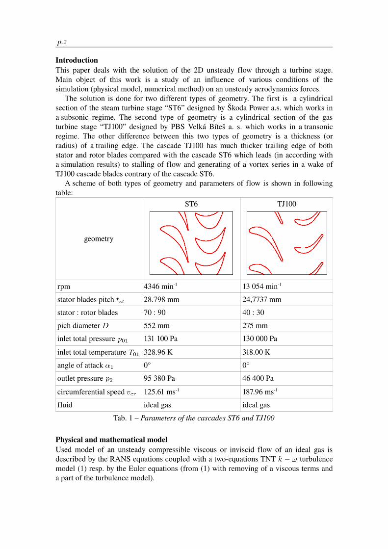
The   scheme   of   the   computational   domain   with   marked   types   of   a boundary conditions   is   shone   in  Fig. 1.  Values  of   the  prescribed  quantities   are  mentioned   in Tab. 1. The total pressure  , the total temperature   and the angle of attack   are prescribed at the inlet boundary. The integral of the static pressure    is prescribed at the outlet boundary. Continuity of the static pressure and desity  is prescribed at  the interface between stator and rotor part (with respect to the time dependent mutual shift of the rotor blades to the stator blades). The velocity vector at the interface respects the circumferential speed  .

Fig. 1 – Scheme of a computational domain

Computational gridThe   structured   quadrilateral   multiblock   grid   with   an   implementation   of   a   block overlapping   (so­called  chimera  grid)   is  used   for  discretization  of   the  computational domain. The grid is combined from the “O”­type blocks around the blades and “H”­type basic blocks (see fig. 2 and fig. 3).

 p.6 

 

Fig. 2 – Computational grid for the ST6 cascade, red – stator part, blue – rotor part

 

Fig. 3 – Computational grid for the TJ100 cascade, red – stator part, blue – rotor part

Colloquium FLUID DYNAMICS 2009Institute of Thermomechanics AS CR, v.v.i., Prague, October 21 ­ 23, 2009

p.7 

Results and discussionA character of a flowfields in a static temperature isolines form in the blades ST6 and TJ100 we can compar in Fig. 4. We can see, that contrary to the cascade ST6 where the trailing edges are relatively sharp in the cascade TJ100 in consequence of thick trailing edges   the  vortex   series  behind   the   stator  blades   is  generated.  Of  course   a  physical correctness   of   this   effect   is   controversial   in   relation   to   used   physical   model   and numerical method (namely the TNT   turbulence model and computational grid). However a presence of a higher frequence effect  in  the flow field make possible  to check an ability of different variants of used physical model and numerical method to represent the higher frequence effect.

ST6 TJ100Fig. 4 – Flow field – static temperatute isolines, left: ST6cascade, right: TJ100 cascade

The properties of used models are presented on a time behaviour of an action of force  and   at stator and rotor blades and their frequency spectrum. The influence 

of the physycal model – viscous tyrbulent and inviscid model is presented in Fig. 5 for the cascade ST6 and Fig. 6 for the cascade TJ100. In both cases the scheme (17) with 2016 physical steps per period for ST6 and 1008 steps per period fos TJ100 was used. We can see a slightly shift of the time behaviour of the forces obtained by the inviscid model against the turbulent model in the cascade ST6 however the spectrums of both models are almost identical (Fig. 5). In the cascade TJ100 we can see slightly increasing of amplitude of higher frequency effect and shift  this  frequency (from 38.000 Hz to 45.000 Hz) for inviscid model against to turbulent model, lower frequency effect are by both models checked almost identycaly.

 p.8 

Fig. 5 – Comparison of viscous turbulent and inviscid model in the cascade ST6,red: inviscid, blue: viscous turbulent

Fig. 6 – Comparison of viscous turbulent and inviscid model in the cascade TJ100, red: inviscid, blue: viscous turbulent

Colloquium FLUID DYNAMICS 2009Institute of Thermomechanics AS CR, v.v.i., Prague, October 21 ­ 23, 2009

p.9 

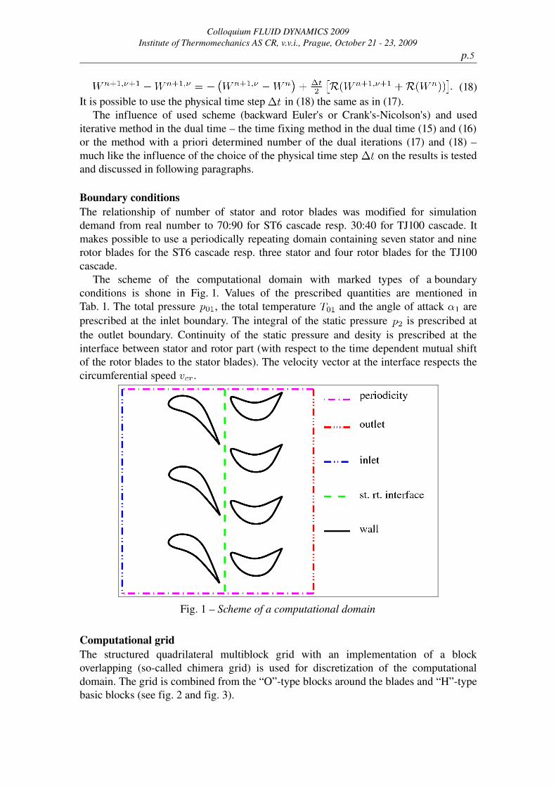
The  influence of used type of   limiter  (Van Albada's  or  Van Leer's)   in  2D linear reconstruction technique is presented in Fig. 7 in the cascade TJ100. The scheme (17) with 1008 physycal steps per period and the inviscid model are used in this case. We can see, that the spectrum in both cases is practically the same, but we can recognize some dissimilarities   in   the   time   behaviours   although   the   difference   between   both   used methods   is  very  small.  This  example   illustrates  a  dependence  of   time behaviour  of quantities in unsteady cases on the space discretization.

Fig. 7 – Influence of type of limiter, red: Van Albada's limiter, blue: Van Leer's limiter

The differece between the second order backward Euler's scheme and the Crank's­Nicolson's scheme is presented in Fig. 8 in the cascade TJ100. The schemes (17) and (18) with 1008 physycal steps per period and the inviscid model are used in this case. We can see that differences between this two schemes are minimal in both time and frequence domain. The Euler's scheme is a bit more robust  in start of solution than Crank's – Nicolson's scheme.

 p.10 

Fig. 8 – Influence of type of time discretization, red: second order backward Euler's  scheme, blue: Crank's­Nicolson's scheme

The   influence   of   choise   of   the   physical   time   step     which   is   joint   with   the circumferential speed   and the number of the physycal steps per period is presented in Fig. 9 for the cascade ST6 with using of the viscous turbulence model and the Euler's schemes (15) or (17) and in Fig. 10 for the cascade TJ100 with using of the inviscid model and the Crank's – Nicolson's schemes (16) or (18). In the cascade ST6 was used 2016 physical steps per period with the Euler's scheme in form (17) or 63 physical steps per period with the Euler's scheme in form (15) with restriction to maximum 30 dual iterations.   In   the  cascade  TJ100  was  used  1008  physycal   steps  per  period  with   the Crank's – Nicolson's  scheme in form (18) or 108 physical steps per period with the Crank's   –   Nicolson's   scheme   in   form   (16)   with   restriction   to   maximum   30   dual iterations.   Using   of   lower   number   of   the   physical   steps   per   period   don't   leads   to acceleration of solution (high number of the dual iterations) but it leads to losse of the accuracy in time. In Fig. 9 we can see that by using of lower number of the physical steps  per  period   is   checked  only   first  major   frequence   (and  partially   second  major frequence for the rotor blades). In Fig. 10 we can see that by using of lower number of the  physical   steps  per  period  are  high   frequence  effect   shifted   from 45.000 Hz  (for invoscid model) to 24.000 Hz.

Colloquium FLUID DYNAMICS 2009Institute of Thermomechanics AS CR, v.v.i., Prague, October 21 ­ 23, 2009

p.11 

Fig. 9 – Influence of physical time step   in cascade ST6, red: 2016 steps per period,  blue: 63 steps per period

Fig. 10 – Influence of physical time step   in cascade TJ100, red: 1008 steps per period, blue: 108 steps per period

 p.12 

ConclusionBy virtue of the simulations of the unsteady stator – rotor interaction in the cascades ST6 and TJ100 by using of various physical models and modifications of numerical methods we can say that using of the iviscid model leads to slightly shift of the mean values of the forces against results obtained by the turbulent model in the cascade ST6. Another result of using of the inviscid model if slightly increase of the frequence of the high­frequence effect in the cascade TJ100.

The results obtained by using of the Van Albada's limiter and the Van Leer's limiter are similar, but this example illustrates a dependence of time behaviour of quantities in unsteady cases on the space discretization.

The second order backward Euler's scheme and the Crank's­Nicolson's scheme give almost the same results, but the Euler's scheme is a bit more robust in start of solution than Crank's – Nicolson's scheme.

Using of lower number of the physical steps per period don't leads to acceleration of solution (high number of the dual iterations) but it leads to losse of the accuracy in time.

AcknowledgementThe work was supported by the project FT­TA5/067 of the Ministry of   Industry and Trade of the Czech Republic. 

References[1] Kok, J. C.: Resolving the Dependence on Freestream Values for    Turbulence Model, AIAA Journal, Vol. 38, No. 7, 2000.

[2] Feistauer M., Felcman J., Straškraba I.: Mathematical and Computational Methods for Compressible Flow. Oxford University Press, 2003.

[3]  Fořt   J.,   Fürst   J.,   Halama   J.,  Kozel  K.,   Louda   P.,   Sváček  P.:   Numerické   řešení nestacionárního   proudění   v   turbínovém   stupni   ST6.   Report   FS   ČVUT   201­08­155, Prague 2008.

[4]   Straka   P.:   Výpočet   nestacionárního   proudění   v   turbínovém   stupni   ST6.   Report VZLÚ R­4476, Prague 2008.