Unsteady Fluid Flow Analysis as Applied to the Internal ... · Unsteady Fluid Flow Analysis as...

Unsteady Fluid Flow Analysis as Applied to the Internal Flow in a Pump using ANSYS CFX

Yasushi Funaba Toshiyuki Sato Satomi Suzuki

Akimitsu Terunuma Takahide Nagahara

Hitachi Plant Technologies, Ltd. (from April this year)

Abstract

Recent years have shown a growth in the utilization of virtual analysis models in the early part of the product development cycle. This approach had been considered a more efficient method of developing a product, since it reduces the number of prototypes required, hence, reducing actual development cost and it expediates market release. Since the introduction of a PC cluster in our company, we had been able to execute larger scale analysis with an increase in calculation speed. It also became possible to analyze the internal flow in a pump using unsteady state with sufficient accuracy. There were some incidents wherein steady state fluid flow prediction in not applicable. This report introduces some examples comparing analysis results with experimental data as applied to some of our company’s products.

Introduction Our company’s main focus is the development, design, production, sale, and aftercare of pumps and blowers used in turbomachinery. Therefore, it was necessary to introduce an accurate analytical code for turbomachinery.

After testing several analytical codes, we concluded that CFX-TASCflow (TASCflow) to be the best and easy to use. Through development and evolution, ANSYS CFX is the present benchmark for turbomachinery. However, some functions of TASCflow have been carried over and is still used in ANSYS CFX. As for the analysis of the turbomachinery in our company, ANSYS CFX is becoming the standard now.

On the other hand, three dimension CAD development is also remarkable, as a result, the mesher tool can automatically make the mesh by using the obtained three dimension shape to a practical level, and it has been able to greatly reduce time and costs that are needed to make the mesh.

A generable mesh in the automatic operation is only the tetra or a mixture of the tetra and the prism in the current state, and ANSYS CFX can use these meshes. Therefore, the operation of this code is comparatively easy, even for an analytical beginner.

Recent years have shown the growth in the utilization of virtual analysis models in the early part of the product development cycle. This approach had been considered a more efficient method of developing a product since it reduces the number of prototypes required, hence, reducing actual development cost and it expediates market release. Since the introduction of a PC cluster in our company, we had been able to execute larger scale analysis with an increase in calculation speed. It also became possible to analyze the internal flow in a pump using unsteady state with sufficient accuracy. There were some incidents, wherein, steady state fluid flow prediction in not applicable.

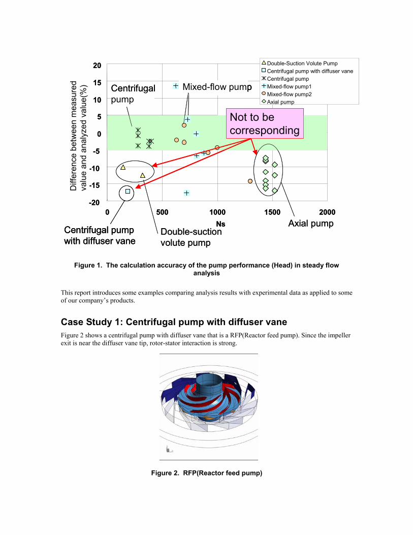
Figure 1 shows the calculation accuracy of the pump performance (Head) in steady flow analysis. It is understood not to be corresponding to the centrifugal pump with diffuser vane, the double-suction volute pump, and the axial pump.

-20

-15

-10

-5

0

5

10

15

20

0 500 1000 1500 2000Ns

実験

値－

計算

値　（

％）

Double-Suction Volute PumpCentrifugal pump with diffuser vaneCentrifugal pumpMixed-flow pump1Mixed-flow pump2Axial pump

Axial pumpDouble-suction volute pump

Centrifugal pump with diffuser vane

Mixed-flow pumpCentrifugal pump

Diff

eren

ce b

etw

een

mea

sure

d va

lue

and

anal

yzed

val

ue(%

)

Not to be corresponding

-20

-15

-10

-5

0

5

10

15

20

0 500 1000 1500 2000Ns

実験

値－

計算

値　（

％）

Double-Suction Volute PumpCentrifugal pump with diffuser vaneCentrifugal pumpMixed-flow pump1Mixed-flow pump2Axial pump


Centrifugal pump with diffuser vaneCentrifugal pump with diffuser vane

Mixed-flow pumpMixed-flow pumpCentrifugal pump

Diff

eren

ce b

etw

een

mea

sure

d va

lue

and

anal

yzed

val

ue(%

)

Not to be corresponding

Figure 1. The calculation accuracy of the pump performance (Head) in steady flow analysis

This report introduces some examples comparing analysis results with experimental data as applied to some of our company’s products.

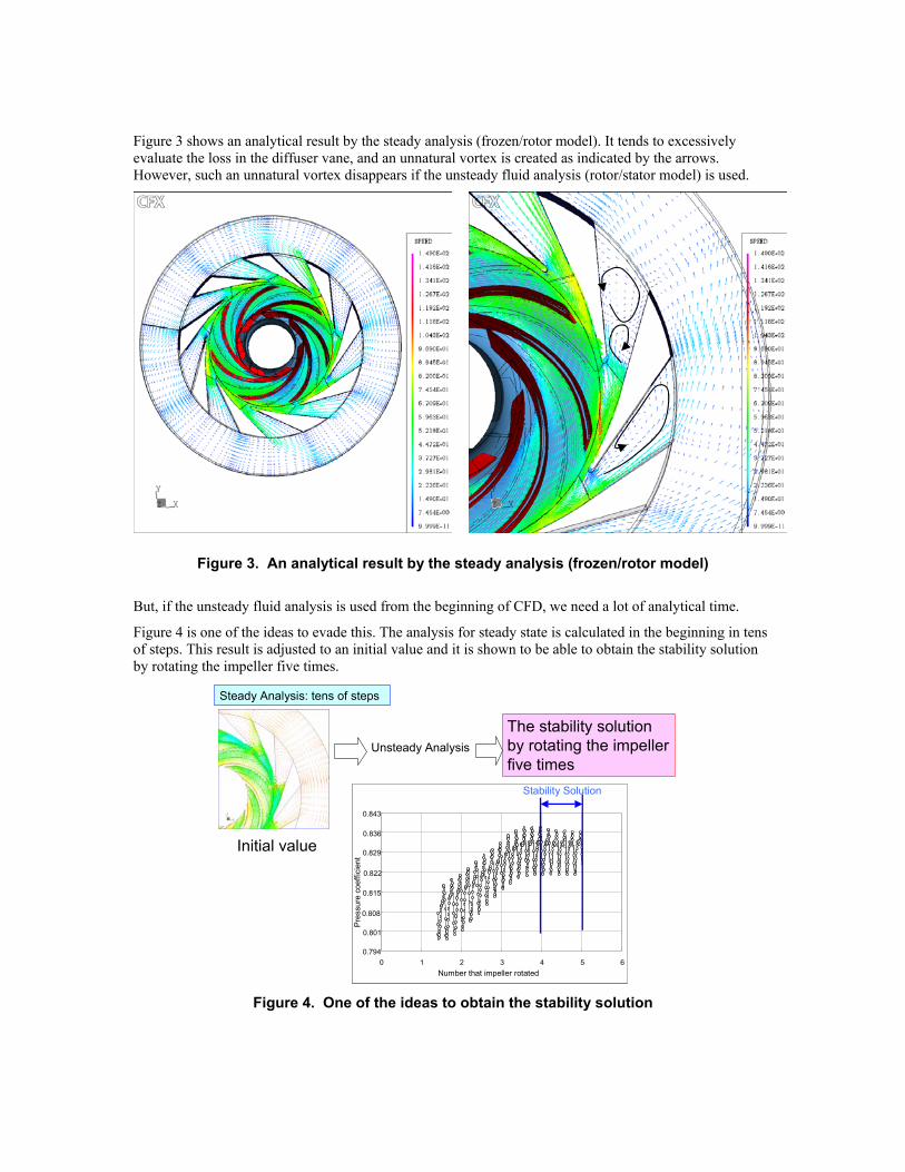
Case Study 1: Centrifugal pump with diffuser vane Figure 2 shows a centrifugal pump with diffuser vane that is a RFP(Reactor feed pump). Since the impeller exit is near the diffuser vane tip, rotor-stator interaction is strong.

Figure 2. RFP(Reactor feed pump)

0.794

0.801

0.808

0.815

0.822

0.829

0.836

0.843

0 1 2 3 4 5 6Number that impeller rotated

Pre

ssur

e co

effic

ient

Stability Solution

0.794

0.801

0.808

0.815

0.822

0.829

0.836

0.843

0 1 2 3 4 5 6Number that impeller rotated

Pre

ssur

e co

effic

ient

Stability Solution

Initial value

Unsteady AnalysisThe stability solution by rotating the impeller five times

Steady Analysis: tens of steps

Figure 3 shows an analytical result by the steady analysis (frozen/rotor model). It tends to excessively evaluate the loss in the diffuser vane, and an unnatural vortex is created as indicated by the arrows. However, such an unnatural vortex disappears if the unsteady fluid analysis (rotor/stator model) is used.

Figure 3. An analytical result by the steady analysis (frozen/rotor model)

But, if the unsteady fluid analysis is used from the beginning of CFD, we need a lot of analytical time.

Figure 4 is one of the ideas to evade this. The analysis for steady state is calculated in the beginning in tens of steps. This result is adjusted to an initial value and it is shown to be able to obtain the stability solution by rotating the impeller five times.

Figure 4. One of the ideas to obtain the stability solution

180deg rotation position 360deg rotation position

Frozen/rotor(100%Q)0.8

0.9

1

1.1

1.2

1.3

1.4

1.5

0 100 200 300 400 500 600 700Rotation angle (deg)

Nor

mar

ized

hea

d

Steady Analysis

Unsteady Analysis

Measurement Value

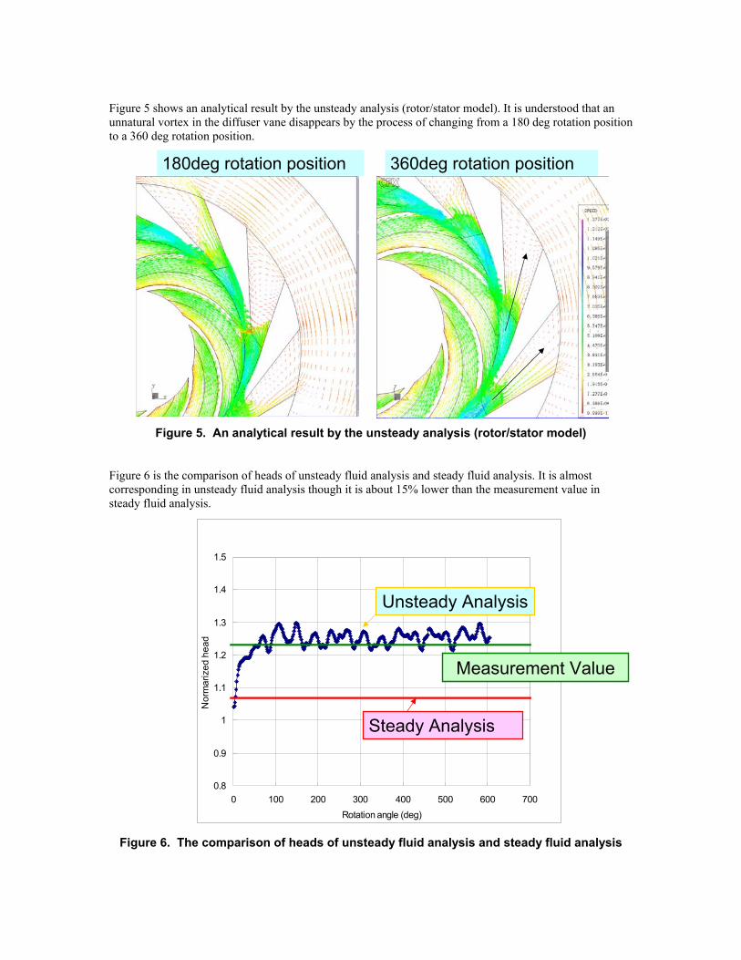
Figure 5 shows an analytical result by the unsteady analysis (rotor/stator model). It is understood that an unnatural vortex in the diffuser vane disappears by the process of changing from a 180 deg rotation position to a 360 deg rotation position.

Figure 5. An analytical result by the unsteady analysis (rotor/stator model)

Figure 6 is the comparison of heads of unsteady fluid analysis and steady fluid analysis. It is almost corresponding in unsteady fluid analysis though it is about 15% lower than the measurement value in steady fluid analysis.

Figure 6. The comparison of heads of unsteady fluid analysis and steady fluid analysis

Impeller

Suction

Discharge

Volute

Case Study 2: Double-Suction Volute Pump Figure 7 shows the structure of double-suction volute pump.

Figure 7. The structure of double-suction volute pump

Example 1: Ns=135 Figure 8 shows a relative position of the blade and a leading edge of the division wall. The flow might be different for steady fluid analysis according to the relative position of the blade and leading edge of the division wall (or Tongue). Figure 9 shows three kinds of blade position. Fluid analyses have been done in 3 positions.

Figure 10 shows an Entire grid and impeller grid. In this example, a non-structural grid was adopted. Figure 11 shows streamlines of analytical result.

Blade position 1 Blade position 2 Blade position 3

Figure 10. Entire grid and impeller grid Figure 11. Streamlines of analytical result

Figure 8. Relative position of blade and leading edge of division wall

Figure 9. Three kinds of blade position

0.8

0.85

0.9

0.95

1

1.05

1.1

1.2

0 10 20 30 40 50 60 70Rotation angle(deg)

Pre

ssur

e C

oeffi

cien

t

1.15

Unsteady analysisSteady analysisMeasurement

1.15

0.8

0.85

0.9

0.95

1

1.05

1.1

1.2


Pre

ssur

e C

oeffi

cien

t

1.15

Unsteady analysisSteady analysisMeasurement1.15


1.15

Pressure Coefficient Normalized Efficiency

0.8

0.85

0.9

0.95

1

1.05

1.1


Nor

mal

ized

Effi

cien

cy


0.8

0.85

0.9

0.95

1

1.05

1.1


Nor

mal

ized

Effi

cien

cy



Steady analysis Unsteady analysisBlade position 1

Figure 12 shows a velocity vector of steady analysis and unsteady analysis. In the steady fluid analysis, an unnatural flow is formed by generating the low flow velocity region, and causing the recirculation in the impeller. Such a flow doesn't exist in unsteady fluid analysis.

Figure 12. Velocity vector of Steady analysis and Unsteady analysis

Figure 13 shows the comparison between a measurement value, steady fluid analysis, and unsteady fluid analysis. It is understood that the accuracy of unsteady fluid analysis is better.

Figure 13. The comparison between a measurement value, steady fluid analysis, and unsteady fluid analysis

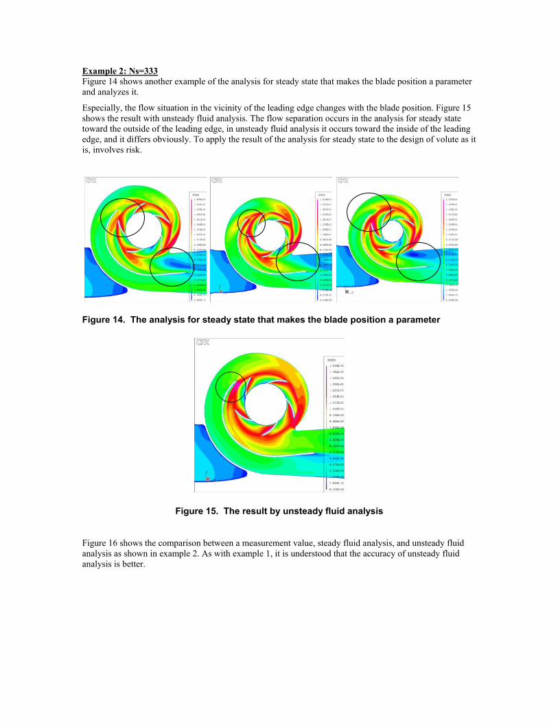
Example 2: Ns=333 Figure 14 shows another example of the analysis for steady state that makes the blade position a parameter and analyzes it.

Especially, the flow situation in the vicinity of the leading edge changes with the blade position. Figure 15 shows the result with unsteady fluid analysis. The flow separation occurs in the analysis for steady state toward the outside of the leading edge, in unsteady fluid analysis it occurs toward the inside of the leading edge, and it differs obviously. To apply the result of the analysis for steady state to the design of volute as it is, involves risk.

Figure 14. The analysis for steady state that makes the blade position a parameter

Figure 15. The result by unsteady fluid analysis

Figure 16 shows the comparison between a measurement value, steady fluid analysis, and unsteady fluid analysis as shown in example 2. As with example 1, it is understood that the accuracy of unsteady fluid analysis is better.

同相羽根車異相羽根車

The in-phase impeller The varying phase impellerOffset arrangement

1.0

1.025

1.05

1.1

1.15

1.2

1.225

1.25

0 10 20 30 40 50 60 70羽根車位置(deg)

全揚

程[m

]

0.89

0.92

0.94

0.97

1.0

1.03

1.06

効率

[%]

Measured pressure coefficient

Measured efficiency

Pre

ssur

e C

oeffi

cien

t

Rotation angle(deg)

Steady analysis, Efficiency

Steady analysis, Pressure coefficient

Unsteady analysis, Efficiency

Unsteady analysis, Pressure coefficient

Nor

mal

ized

Effi

cien

cy1.175

1.125

1.075

1.0

1.025

1.05

1.1

1.15

1.2

1.225

1.25

0 10 20 30 40 50 60 70羽根車位置(deg)

全揚

程[m

]

0.89

0.92

0.94

0.97

1.0

1.03

1.06

効率

[%]


Measured efficiency

Pre

ssur

e C

oeffi

cien

t

Rotation angle(deg)

Steady analysis, Efficiency


Unsteady analysis, Efficiency

Unsteady analysis, Pressure coefficient

Nor

mal

ized

Effi

cien

cy1.175

1.125

1.075


Figure 17 shows the difference of double-suction volute pump which is the in-phase impeller and the varying phase impeller. Figure 18 is a result of these unsteady fluid analyses.

The varying phase impeller shows double the frequency in the number of blades with the in-phase impeller, and it is understood that the amplitude of the pressure change is about a half. The varying phase impeller has the possibility to decrease noise and vibration more than the in-phase impeller.

Figure 17. The difference between double-suction volute pump which is the in-phase impeller and the varying phase impeller

Guide vane(10)

Impeller(3)

A A

The in-phase impeller

The amplitude of the pressure change is large

The varying phase impeller

The amplitude of the pressure change is small

Analysis step

全揚

程[m

]

23

23.5

24

24.5

1 21 41 61 81 101 121

1.175

1.25

1.2

1.15

Pre

ssur

e C

oeffi

cien

t

Analysis step

全揚

程[m

]

23

23.5

24

24.5

1 21 41 61 81 101 121

1.175

1.25

1.2

1.15

Pre

ssur

e C

oeffi

cien

tMeasured, in-phase impeller

Measured, varying phase impeller

Analysis, in-phase impeller

Analysis, varying phase impeller

Figure 18. The comparison of head fluctuations between the in-phase impeller and the varying phase impeller

Case Study 3: Axial Pump Figure 19 shows the structural chart of the axial pump. Figure 20 is the comparison of the steady fluid analysis and the unsteady fluid analysis for the secondary flow in an A-A section. When using unsteady fluid analysis the flow was almost identical, however when using steady fluid analysis the flow became irregular and was unnatural as a whole.

Figure 19. Structure of the axial pump

0.8

0.85

0.9

0.95

1

1.05

1.1

1.15

1.2

0 50 100 150 200

Analysis step

Pre

ssur

e C

oeffi

cien

t



Unsteady analysis,

Pressure coefficient

Secondary flow in guide vane

Almost identical Section A-A

Irregular Section A-A

Steady Analysis Unsteady Analysis

Vortices are generated

Figure 20. The comparison of the steady fluid analysis and the unsteady fluid analysis

Figure 21 shows the comparison between a measurement value, steady fluid analysis, and unsteady fluid analysis. It is understood that the accuracy of unsteady fluid analysis is better.


-20

-15

-10

-5

0

5

10

15

20

0 500 1000 1500 2000Ns

実験

値－

計算

値　（

％）


Centrifugal pump with diffuser vane

Mixed-flow pump

Centrifugal pump

Diff

eren

ce b

etw

een

mea

sure

d va

lue

and

anal

yzed

val

ue(%

)

Double-Suction Volute PumpDouble-Suction Volute Pump (Unsteady)Centrifugal pump with diffuser vaneCentrifugal pump with diffuser vane (Unsteady)Centrifugal pumpMixed-flow pump1Mixed-flow pump2Axial pumpAxial pump (Unsteady)

-20

-15

-10

-5

0

5

10

15

20

0 500 1000 1500 2000Ns

実験

値－

計算

値　（

％）


Centrifugal pump with diffuser vaneCentrifugal pump with diffuser vane

Mixed-flow pumpMixed-flow pump

Centrifugal pump

Diff

eren

ce b

etw

een

mea

sure

d va

lue

and

anal

yzed

val

ue(%

)



Conclusion The analysis for steady state on the centrifugal pump with a diffuser vane, double-suction volute pump, and axial pump might not be corresponding to the measurement value. Therefore, the unsteady fluid analysis was applied in these cases. Figure 22 shows the results. By using the unsteady fluid analysis from this figure, we can obtain data which is sufficiently accurate to use as a guidepost for design.

Figure 22. Improvement of accuracy by the unsteady fluid analysis

Unsteady Fluid Flow Analysis as Applied to the Internal ... · Unsteady Fluid Flow Analysis as...

Documents

Transcript of Unsteady Fluid Flow Analysis as Applied to the Internal ... · Unsteady Fluid Flow Analysis as...