Unsteady Flow in Pipe Networks

lecure notes

Csaba Hos Laszlo Kullmann Botond Erdos Viktor Szabo

March 27, 2014

1

Contents

1 A few numerical techniques in a nutshell 4

1.1 Solving systems of algebraic equtions . . . . . . . . . . . . . . . . . . . . . . . . . . . . 4

1.2 Estimating derivatives with finite differences . . . . . . . . . . . . . . . . . . . . . . . . 6

1.3 Solving ordinary differential equations . . . . . . . . . . . . . . . . . . . . . . . . . . . 8

2 Calculation of the wave speed under different circumstances 15

3 Model of a ventilation channel with rectangular cross-section 17

3.1 Boundary conditions . . . . . . . . . . . . . . . . . . . . . . . . . . . . . . . . . . . . . 18

4 Unsteady 1D slightly incompressible fluid flow 22

4.1 Governing equations . . . . . . . . . . . . . . . . . . . . . . . . . . . . . . . . . . . . . 22

4.2 Application on pressurized liquid pipeline systems . . . . . . . . . . . . . . . . . . . . 22

5 Impedance method 27

5.1 Basic theory . . . . . . . . . . . . . . . . . . . . . . . . . . . . . . . . . . . . . . . . . . 27

5.2 Boundary conditions . . . . . . . . . . . . . . . . . . . . . . . . . . . . . . . . . . . . . 30

6 Unsteady 1D open-surface flow in prismatic channel 32

6.1 Introduction . . . . . . . . . . . . . . . . . . . . . . . . . . . . . . . . . . . . . . . . . . 32

6.2 Continuity equation and equation motion for open-surface flow . . . . . . . . . . . . . 32

6.3 The Saint-Venant equations . . . . . . . . . . . . . . . . . . . . . . . . . . . . . . . . . 34

6.4 Open-surface channel flow and gas dynamics . . . . . . . . . . . . . . . . . . . . . . . 34

6.5 Method of characteristics for open-surface flow . . . . . . . . . . . . . . . . . . . . . . 35

7 Unsteady 1D compressible gas flow 39

7.1 Governing equations . . . . . . . . . . . . . . . . . . . . . . . . . . . . . . . . . . . . . 39

7.2 Isentropic MOC . . . . . . . . . . . . . . . . . . . . . . . . . . . . . . . . . . . . . . . . 40

7.3 Boundary conditions . . . . . . . . . . . . . . . . . . . . . . . . . . . . . . . . . . . . . 41

7.4 The Lax-Wendroff scheme . . . . . . . . . . . . . . . . . . . . . . . . . . . . . . . . . . 43

2

8 General framework on characteristic lines of PDEs 45

8.1 Solution of general partial differential equations describing fluid flow . . . . . . . . . . 45

8.2 Classification of second order linear PDEs with constant coefficients. Canonical form

and characteristic differential equation of 2nd order PDE-s. . . . . . . . . . . . . . . . 46

8.3 Coordinate transformation resulting in a simpler form of operator L . . . . . . . . . . 48

9 Steady 2D supersonic gas flow (in the diffuser part of a Laval nozzle) 51

3

1 A few numerical techniques in a nutshell

1.1 Solving systems of algebraic equtions

Consider the problem of finding the solution of

f(x) = 0, (1)

where f is some (complicated) nonlinear function.

In the 1D case, Newton’s technique (or sometime called Netwon-Raphson technique) improves

the previous solution xn by finding the intersection of the x axes and the tangent line of the function

evaluated at xn:

f ′(xn) ≈ ∆y

∆x=

f(xn)

xn − xn+1→ xn+1 = xn −

f(xn)

f ′(xn). (2)

In the multidimensional case, we have

xn+1 = xn −(f ′(xn)

)−1f(xn). (3)

Newton’s method is an extremely powerful technique, in general the convergence is quadratic: as

the method converges on the root, the difference between the root and the approximation is squared

(the number of accurate digits roughly doubles) at each step. However, there are some difficulties with

the method.

Difficulty in calculating derivative of a function Newton’s method requires that the derivative

is calculated directly. An analytical expression for the derivative may not be easily obtainable

and could be expensive to evaluate. In these situations, it may be appropriate to approximate

the derivative by using the slope of a line through two nearby points on the function, e.g.

f ′(xn) ≈ f(xn + ∆x)− f(xn)

∆x, with e.g. ∆xn = 0.01xn. (4)

Failure of the method to converge to the root Sometimes the technique runs into an infinte

loop. In such cases relaxation may help, i.e. we require the method to improve the solution

only partially:

xn+1 = xn − ωf(xn)

f ′(xn), with 0 ≤ ω ≤ 1. (5)

Overshoot If the first derivative is not well behaved in the neighborhood of a particular root, the

method may overshoot, and diverge from that root. Furthermore, if a stationary point of the

function is encountered, the derivative is zero and the method will terminate due to division by

zero. Use relaxation in such cases.

4

Poor initial estimate A large error in the initial estimate can contribute to non-convergence of the

algorithm.

Mitigation of non-convergence In a robust implementation of Newton’s method, it is common to

place limits on the number of iterations, bound the solution to an interval known to contain the

root, and combine the method with a more robust root finding method.

Slow convergence for roots of multiplicity > 1 If the root being sought has multiplicity greater

than one, the convergence rate is merely linear (errors reduced by a constant factor at each step)

unless special steps are taken. When there are two or more roots that are close together then it

may take many iterations before the iterates get close enough to one of them for the quadratic

convergence to be apparent. However, if the multiplicity m of the root is known, one can use the

following modified algorithm that preserves the quadratic convergence rate:

xn+1 = xn −mf(xn)

f ′(xn). (6)

•

Note that Newton’s technique is directly applicable to complex-valued functions. An interesting

and beautiful experiment is to color the complex plane based on the basin of attraction of the roots

of a complex polinomial function, say, x5 − 1 = 0, giving rise to fractals.

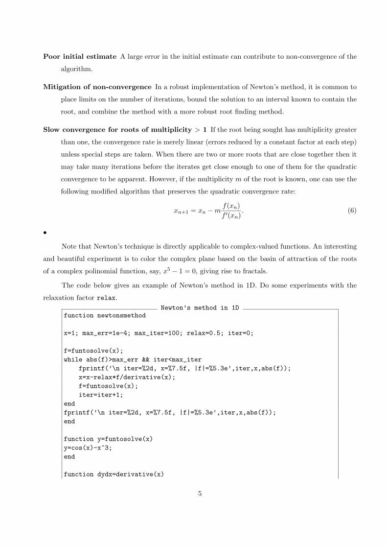
The code below gives an example of Newton’s method in 1D. Do some experiments with the

relaxation factor relax.

Newton’s method in 1Dfunction newtonsmethod

x=1; max_err=1e-4; max_iter=100; relax=0.5; iter=0;

f=funtosolve(x);

while abs(f)>max_err && iter<max_iter

fprintf(’\n iter=%2d, x=%7.5f, |f|=%5.3e’,iter,x,abs(f));

x=x-relax*f/derivative(x);

f=funtosolve(x);

iter=iter+1;

end

fprintf(’\n iter=%2d, x=%7.5f, |f|=%5.3e’,iter,x,abs(f));

end

function y=funtosolve(x)

y=cos(x)-x^3;

end

function dydx=derivative(x)

5

dydx=-sin(x)-3*x^2;

end

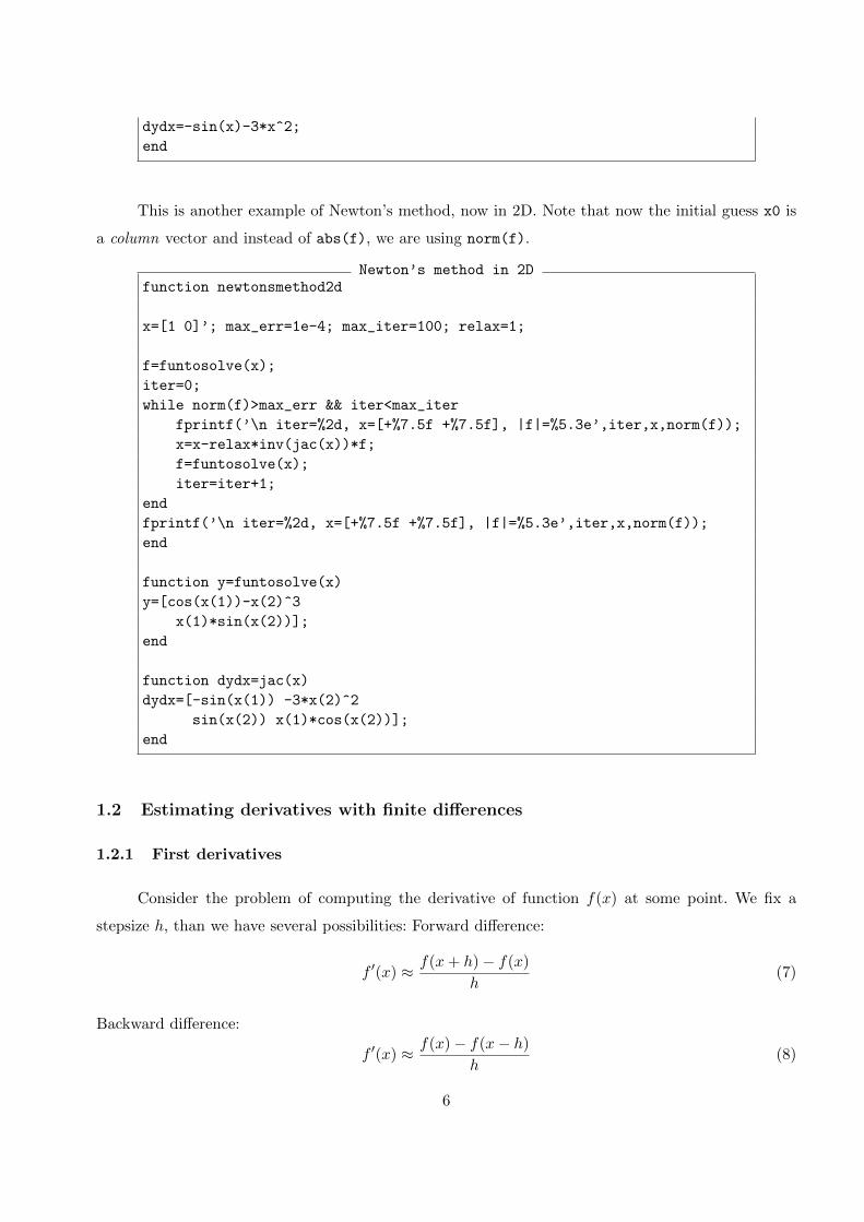
This is another example of Newton’s method, now in 2D. Note that now the initial guess x0 is

a column vector and instead of abs(f), we are using norm(f).

Newton’s method in 2Dfunction newtonsmethod2d

x=[1 0]’; max_err=1e-4; max_iter=100; relax=1;

f=funtosolve(x);

iter=0;

while norm(f)>max_err && iter<max_iter

fprintf(’\n iter=%2d, x=[+%7.5f +%7.5f], |f|=%5.3e’,iter,x,norm(f));

x=x-relax*inv(jac(x))*f;

f=funtosolve(x);

iter=iter+1;

end

fprintf(’\n iter=%2d, x=[+%7.5f +%7.5f], |f|=%5.3e’,iter,x,norm(f));

end

function y=funtosolve(x)

y=[cos(x(1))-x(2)^3

x(1)*sin(x(2))];

end

function dydx=jac(x)

dydx=[-sin(x(1)) -3*x(2)^2

sin(x(2)) x(1)*cos(x(2))];

end

1.2 Estimating derivatives with finite differences

1.2.1 First derivatives

Consider the problem of computing the derivative of function f(x) at some point. We fix a

stepsize h, than we have several possibilities: Forward difference:

f ′(x) ≈ f(x+ h)− f(x)

h(7)

Backward difference:

f ′(x) ≈ f(x)− f(x− h)

h(8)

6

10−6

10−4

10−2

100

10−15

10−10

10−5

100

Step size h

Re

lative

err

or

FD

BD

3pt CD

5pt CD ~h

~h2

~h4

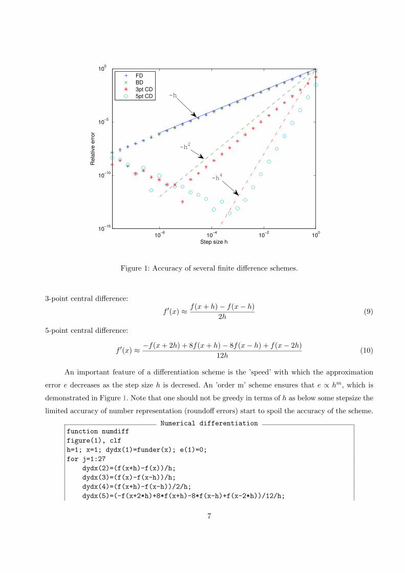
Figure 1: Accuracy of several finite difference schemes.

3-point central difference:

f ′(x) ≈ f(x+ h)− f(x− h)

2h(9)

5-point central difference:

f ′(x) ≈ −f(x+ 2h) + 8f(x+ h)− 8f(x− h) + f(x− 2h)

12h(10)

An important feature of a differentiation scheme is the ’speed’ with which the approximation

error e decreases as the step size h is decresed. An ’order m’ scheme ensures that e ∝ hm, which is

demonstrated in Figure 1. Note that one should not be greedy in terms of h as below some stepsize the

limited accuracy of number representation (roundoff errors) start to spoil the accuracy of the scheme.

Numerical differentiationfunction numdiff

figure(1), clf

h=1; x=1; dydx(1)=funder(x); e(1)=0;

for j=1:27

dydx(2)=(f(x+h)-f(x))/h;

dydx(3)=(f(x)-f(x-h))/h;

dydx(4)=(f(x+h)-f(x-h))/2/h;

dydx(5)=(-f(x+2*h)+8*f(x+h)-8*f(x-h)+f(x-2*h))/12/h;

7

for i=2:length(dydx)

e(i)=abs((dydx(1)-dydx(i))/dydx(1));

end

loglog(h,e(2),’+’,h,e(3),’x’,h,e(4),’*’,h,e(5),’o’), hold on

h=h/2;

end

hh=[1 1e-6];

loglog(hh,hh,’-’,hh,hh.^2,’--’,hh,hh.^4,’-.’), hold off

xlabel(’Step size h’), ylabel(’Relative error’)

legend(’FD’,’BD’,’3pt CD’,’5pt CD’,2), axis([0 1 1e-15 1])

end

function y=f(x)

y=sin(x);

end

function dydx=funder(x)

dydx=cos(x);

end

1.2.2 Second derivatives

The simplest possibility is to use the central difference scheme at the half grid points (second-

order accuracy):

f ′′(x) ≈f ′(x+ h

2

)− f ′

(x− h

2

)∆h

=1

h

(f(x+ h)− f(x)

h− f(x)− f(x− h)

h

)=f(x+ h)− 2f(x) + f(x− h)

h2(11)

Another scheme using five points providing fourth-order accuracy is

f ′′(x) ≈ −f(x+ 2h) + 16f(x+ h)− 30f(x) + 16f(x− h)− f(x− 2h)

12h2. (12)

1.3 Solving ordinary differential equations

In general a system of ordinary differential equations (ODEs) have the form of

x′ = f (x, t) , (13)

where the function x(t) is to be determined. In the case when the function f is only dependent upon

t implicitly, that is f = f(x), the ODE is called autonomous, otherwise it is called non-autonomous.

There are two main groups of problems that can be described by ODEs:

8

• Boundary value problems (BVPs), where the function values at the boundaries (x(a) and x(b))

are prescribed. These are usually describing a problem where the independent variables are space

coordinates.

• Initial value problems (IVPs), where the function values are given at an initial time (x(t0)).

These are usually describing problems where the independent variable is time. (In this subject

we mainly deal with IVPs.)

In most of the cases there is no known analytical solution for an IVP. In these cases one tries to

find a numerical approximation for the solution function (x(t)). All these numerical methods are

common in the sense that they give an approximate formula for the time derivative (x) and calculate

the approximate solution at distinct time steps (xn(tn)). Here three basic methods will be presented

briefly.

1.3.1 Explicit Euler method

The basic equation reads:

x ≈ x(t+ ∆t)− x(t)

∆t=xn+1 − xn

∆t= f(xn, tn), (14)

thus in every new time step the new function value can be computed by the formula:

xn+1 = xn + ∆tf(xn, tn). (15)

This method is explicit since the new function value (xn+1) can be explicitly expressed with the help

of the previous values (xn), hence it is fast. On the other hand it is very unstable and inaccurate (first

order method), so in general it is not used. One way to improve the method is to use implicit Euler

method.

1.3.2 Implicit or backward Euler method

The basic equation reads:

x ≈xn+1 − xn

∆t= f(xn+1, tn+1). (16)

This method is implicit, since for every new time step one has to solve a system of algebraic equations

to get xn+1. This can be performed for example by the previously presented Newton’s method. One

advantage of the method is its stability (see Section 1.3.4), however its accuracy is not improved (first

order method). One way to develop the accuracy is to use a higher order scheme such as Runge-Kutta

4.

9

1.3.3 Runge-Kutta 4 method

The basic equation reads:

xn+1 = xn + ∆t

[k1

6+k2

3+k3

3+k4

6

], (17)

with

k1 = f (xn, tn) ,

k2 = f

(xn +

∆t

2k1, tn +

∆t

2

),

k3 = f

(xn +

∆t

2k2, tn +

∆t

2

),

k4 = f (xn + ∆tk3, tn + ∆t) .

This method is fourth order as it is denoted in its name. This means a great improvement in its

accuracy over the Euler method. Since it is an explicit scheme it is fast as well.

1.3.4 Stability

Stability is a very important property of the different kinds of ODE solvers. The common way

of investigating a method’s stability is to consider the following scalar ODE:

x = λx, where λ ∈ C and <(λ) < 0. (18)

The condition <(λ) < 0 is required since we want to deal with a ’normal physical phenomenon’ that

is stable and only the numerical method can introduce instability in the solution. If we apply the

different schemes to (18) we get the following geometric series:

• Explicit Euler method: xn+1 = (1 + ∆tλ)xn

• Implicit Euler method: xn+1 = 11−∆tλxn

• Runge-Kutta 4 method: xn+1 =(

∆tλ+ (∆tλ)2

2! + (∆tλ)3

3! + (∆tλ)4

4!

)xn

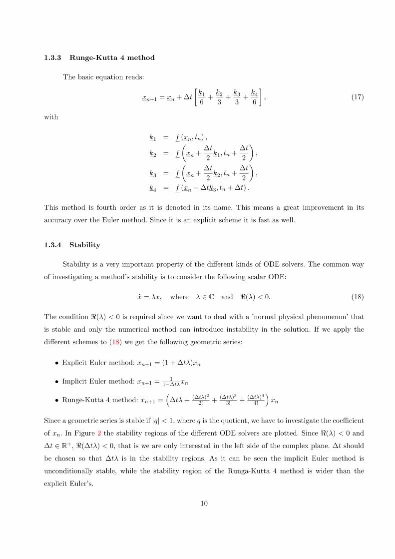
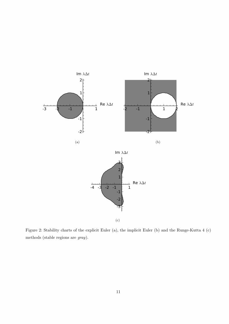
Since a geometric series is stable if |q| < 1, where q is the quotient, we have to investigate the coefficient

of xn. In Figure 2 the stability regions of the different ODE solvers are plotted. Since <(λ) < 0 and

∆t ∈ R+, <(∆tλ) < 0, that is we are only interested in the left side of the complex plane. ∆t should

be chosen so that ∆tλ is in the stability regions. As it can be seen the implicit Euler method is

unconditionally stable, while the stability region of the Runga-Kutta 4 method is wider than the

explicit Euler’s.

10

-3 -2 -1 1Re λ∆t

-2

-1

1

2

Im λ∆t

(a)

-2 -1 1 2Re λ∆t

-2

-1

1

2

Im λ∆t

(b)

-4 -3 -2 -1 1Re λ∆t

-3

-2

-1

1

2

3

Im λ∆t

(c)

Figure 2: Stability charts of the explicit Euler (a), the implicit Euler (b) and the Runge-Kutta 4 (c)

methods (stable regions are gray).

11

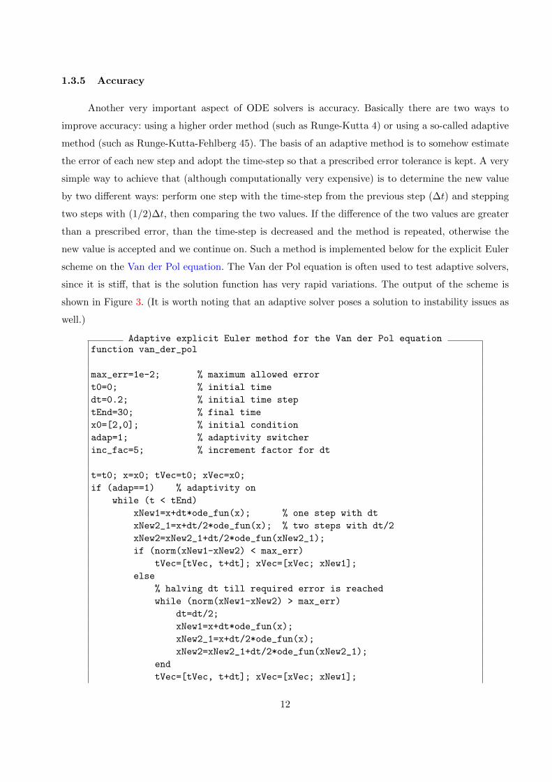
1.3.5 Accuracy

Another very important aspect of ODE solvers is accuracy. Basically there are two ways to

improve accuracy: using a higher order method (such as Runge-Kutta 4) or using a so-called adaptive

method (such as Runge-Kutta-Fehlberg 45). The basis of an adaptive method is to somehow estimate

the error of each new step and adopt the time-step so that a prescribed error tolerance is kept. A very

simple way to achieve that (although computationally very expensive) is to determine the new value

by two different ways: perform one step with the time-step from the previous step (∆t) and stepping

two steps with (1/2)∆t, then comparing the two values. If the difference of the two values are greater

than a prescribed error, than the time-step is decreased and the method is repeated, otherwise the

new value is accepted and we continue on. Such a method is implemented below for the explicit Euler

scheme on the Van der Pol equation. The Van der Pol equation is often used to test adaptive solvers,

since it is stiff, that is the solution function has very rapid variations. The output of the scheme is

shown in Figure 3. (It is worth noting that an adaptive solver poses a solution to instability issues as

well.)

Adaptive explicit Euler method for the Van der Pol equationfunction van_der_pol

max_err=1e-2; % maximum allowed error

t0=0; % initial time

dt=0.2; % initial time step

tEnd=30; % final time

x0=[2,0]; % initial condition

adap=1; % adaptivity switcher

inc_fac=5; % increment factor for dt

t=t0; x=x0; tVec=t0; xVec=x0;

if (adap==1) % adaptivity on

while (t < tEnd)

xNew1=x+dt*ode_fun(x); % one step with dt

xNew2_1=x+dt/2*ode_fun(x); % two steps with dt/2

xNew2=xNew2_1+dt/2*ode_fun(xNew2_1);

if (norm(xNew1-xNew2) < max_err)

tVec=[tVec, t+dt]; xVec=[xVec; xNew1];

else

% halving dt till required error is reached

while (norm(xNew1-xNew2) > max_err)

dt=dt/2;

xNew1=x+dt*ode_fun(x);

xNew2_1=x+dt/2*ode_fun(x);

xNew2=xNew2_1+dt/2*ode_fun(xNew2_1);

end

tVec=[tVec, t+dt]; xVec=[xVec; xNew1];

12

end

t=t+dt; x=xNew1; dt=dt*inc_fac;

end

elseif (adap==0) % adaptivity off

while (t < tEnd)

xNew=x+dt*ode_fun(x);

tVec=[tVec, t+dt]; xVec=[xVec; xNew];

t=t+dt; x=xNew;

end

end

plot(tVec,xVec(:,1),’.-’); xlabel(’t [s]’); ylabel(’displacement [m]’)

function dxdt=ode_fun(x) % Van der Pol equation with mu=5

dxdt(1)=5*(x(1)-1/3*x(1)^3-x(2));

dxdt(2)=1/5*x(1);

13

0 5 10 15 20 25 30 35−3

−2

−1

0

1

2

3

t [s]

dis

pla

cem

en

t [m

]

(a)

0 5 10 15 20 25 30 35−2.5

−2

−1.5

−1

−0.5

0

0.5

1

1.5

2

2.5

t [s]

dis

pla

ce

me

nt [m

]

(b)

Figure 3: Computed displacement of the Van der Pol equation with regular (a) and with adaptive (b)

solvers

14

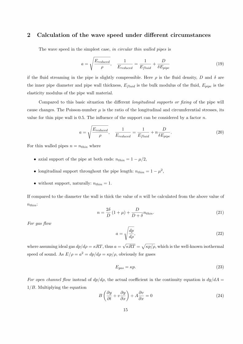
2 Calculation of the wave speed under different circumstances

The wave speed in the simplest case, in circular thin walled pipes is

a =

√Ereduced

ρ,

1

Ereduced=

1

Efluid+

D

δEpipe(19)

if the fluid streaming in the pipe is slightly compressible. Here ρ is the fluid density, D and δ are

the inner pipe diameter and pipe wall thickness, Efluid is the bulk modulus of the fluid, Epipe is the

elasticity modulus of the pipe wall material.

Compared to this basic situation the different longitudinal supports or fixing of the pipe will

cause changes. The Poisson-number µ is the ratio of the longitudinal and circumferential stresses, its

value for thin pipe wall is 0.5. The influence of the support can be considered by a factor n.

a =

√Ereduced

ρ,

1

Ereduced=

1

Efluid+ n

D

δEpipe. (20)

For thin walled pipes n = nthin where

• axial support of the pipe at both ends: nthin = 1− µ/2,

• longitudinal support throughout the pipe length: nthin = 1− µ2,

• without support, naturally: nthin = 1.

If compared to the diameter the wall is thick the value of n will be calculated from the above value of

nthin:

n =2δ

D(1 + µ) +

D

D + δnthin. (21)

For gas flow

a =

√dp

dρ, (22)

where assuming ideal gas dp/dρ = κRT , thus a =√κRT =

√κp/ρ, which is the well-known isothermal

speed of sound. As E/ρ = a2 = dp/dρ = κp/ρ, obviously for gases

Egas = κp. (23)

For open channel flow instead of dp/dρ, the actual coefficient in the continuity equation is dy/dA =

1/B. Multiplying the equation

B

(∂y

∂t+ v

∂y

∂x

)+A

∂v

∂x= 0 (24)

15

with ρ/A and introducing the gravitational acceleration g:

B

Ag

(∂ρgy

∂t+ v

∂ρgy

∂x

)+ ρ

∂v

∂x= 0. (25)

This equation has the same dimension as the earlier continuity equations from which B/(Ag) = 1/a2,

thus the free surface wave speed is

a =

√Ag

B. (26)

In air conditioning the ventilation channels often have rectangular cross section bended from thin

metal plates. These, 1-2 m long channel segments are fixed to each other. Experiments with standing

waves have proved that in this case the wave speed a strongly depends on the angular frequency ω of

the pressure wave. This leads to its dispersion. The a(ω) function has the form:

a(ω) =c√

1 + ρc2f(ω), (27)

where c is the isentropic sound velocity in free air, the function f(ω) depends on the geometry and

material properties of the channel. L is the dimension of the channel side, δ is the thickness of channel

wall:

f(ω) =2L3

Ewallδ3Ω5

(2

cot Ω + coth Ω− Ω

), and Ω = 4

√3ρL4ω2

4Ewallδ2. (28)

The wave speed in liquids strongly depends on free gas content. The wave speed in gaseous fluids

can drop up to a few 10m/s-s although the wave speed in pure normal air is 340m/s. The mixture

characterized by void fraction α = Vg/V is composed of free gas of density ρg and fluid of density ρf

(naturally 1 − α = Vf/V ). The mass of the mixture is ρgVg + ρfVf = ρV . Dividing this by the total

volume V of the mixture and introducing the above abbreviation for the void fraction α the mean

density is: ρ = αρg + (1 − α)ρf . Now the wave speed must be calculated from the mean density and

reduced elasticity modulus. The elasticity will also depend on the compressibility of the gas. By the

definition of the elasticity modulus (Hooks law) dVg = −Vg/Egdp, and dVf = −Vf/Efdp. The total

change of volume V is

dV = dVg + dVf = −(αV

Eg+

(1− α)V

Ef

)dp = −

(α

Eg+

(1− α)

Ef

)V dp (29)

and thus the reduced elasticity modulus Ee is

Ee = −V dp

dV=

1(αEg

+ (1−α)Ef

) . (30)

Finally the square of the wave speed (considering that the extension of the pipe wall compared to the

compressibility of gas content is negligible):

a2 =Eeρ

=1(

αEg

+ (1−α)Ef

)(αρg + (1− α)ρf )

=1(

ακp + (1−α)

Ef

)(αρg + (1− α)ρf )

, (31)

16

as Eg = κRTρ = κp (see above). This rather complicated formula can be simplified realizing that in

the denominator in the first bracket the first, in the second bracket the second term is dominant

a =

√Eeρ≈√

κp

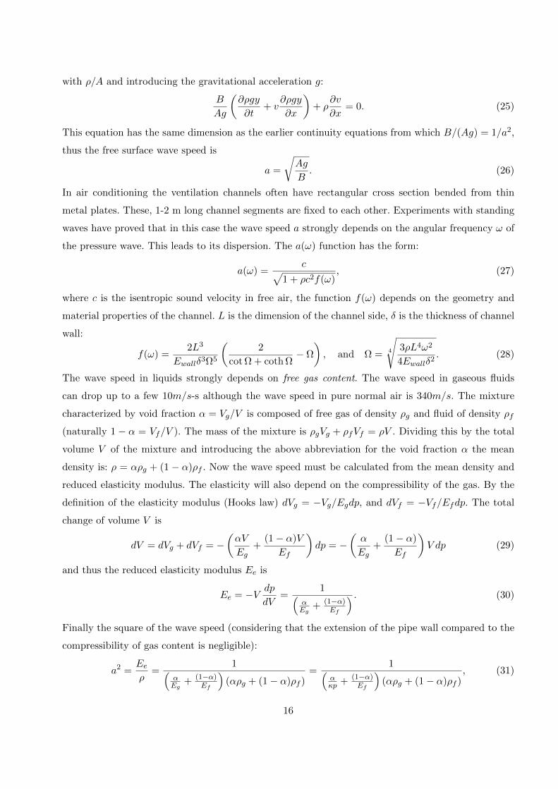
α(1− α)ρf. (32)

Differentiating Eq. (32) with respect to α gives the minimum of the wave speed at α = 0.5.

Figure 4: Wave speed in water containing air at 3 bar pressure

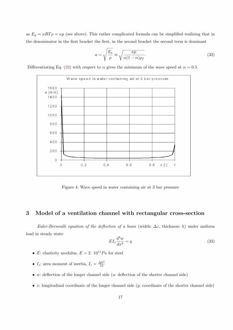
3 Model of a ventilation channel with rectangular cross-section

Euler-Bernoulli equation of the deflection of a beam (width: ∆z, thickness: h) under uniform

load in steady state:

EIzd4w

dx4= q (33)

• E: elasticity modulus, E = 2 · 1011Pa for steel

• Iz: area moment of inertia, Iz = ∆h3

12

• w: deflection of the longer channel side (u: deflection of the shorter channel side)

• x: longitudinal coordinate of the longer channel side (y: coordinate of the shorter channel side)

17

Figure 5: Wave speed in water containing air at 3 bar pressure

The above differential equation for constant load q (force per unit length, q = dp∆z where dp is the

change of overpressure in the channel) is:

EIzd4w

dx4= dp∆z or

d4w

dx4=dp∆z

EIz

denoted= P. (34)

The general solution of this differential equation is

w(x) = Px4

24+ C3

x3

6+ C2

x2

2+ C1x+ C0 (35)

As we suppose symmetry with respect to the centreline of the beam (at x = 0) the terms of uneven

order will drop:

w(x) = Px4

24+ C2

x2

2+ C0 (36)

and similarly

u(x) = Py4

24+D2

y2

2+D0 (37)

for the shorter side of the channel.

3.1 Boundary conditions

The corners are fixed: w(L/2) = 0 and u(−B/2) = 0. The tangents of the channel sides at

the corner are perpendicular as the angle of the corner keeps its value 90: w′′(L/2) = u′′(−B/2).

Denoting the side ratio of the rectangular cross section by s = B/L the solutions satisfying the

boundary conditions are

w(x) = Px4

24+PL2

24

(2s2 − 2s− 1

) x2

2+PL4

8 · 24

(1

2+ 2s− 2s2

), (38)

u(y) = Py4

24+PL2

24

(−s2 − 2s+ 2

) y2

2+PL4

8 · 24s2

(−2 + 2s+

s2

2

). (39)

18

The area change dA of the cross section A = BH is the sum of the integrals of the deflections of the

for side walls:

dA = 2

∫ x=L2

x=−L2

w(x)dx+ 2

∫ y= sL2

y=− yL2

w(y)dy =PL5

24

s5 + 5(s4 − s3 − s2 + s

)+ 1

15. (40)

If both the gas is compressible and the channel area is changing under the pressure change the equation

of continuity is

∂(ρA)

∂t+∂(ρAv)

∂x=∂(ρA)

∂t+ v

∂(ρA)

∂x+ ρA

∂v

∂x=d(ρA)

dp

(∂p

∂t+ v

∂p

∂x

)+ ρA

∂v

∂x= 0. (41)

After some calculations and introducing the isentropic wave velocity c in the gas we have

1

ρA

(Adρ

dp+ ρ

dA

dp

)(∂p

∂t+ v

∂p

∂x

)+∂v

∂x=

(1

ρc2+

1

A

dA

dp

)(∂p

∂t+ v

∂p

∂x

)+∂v

∂x

denoted=

(1

ρc2+ Φ

)(∂p

∂t+ v

∂p

∂x

)+∂v

∂x=

(1

ρa2

)(∂p

∂t+ v

∂p

∂x

)+∂v

∂x= 0. (42)

The wave velocity in the channel denoted above by a is

a =c√

1 + ρc2Φwith Φ =

1

A

dA

dp=

L3

15Eh3

s5 + 5(s4 − s3 − s2 + s

)+ 1

2s, (43)

where ρ is the density of air at the given air temperature. Here a = 173, 4m/s if the air density is

ρ = 1, 2kg/m3 and c = 340m/s with other parameters given at the end of this section.

Experiments have not proved these formulae. Why? Because the channel side walls have a mass

and one has to consider the inertia of this mass. The equation of dynamic bending of a slender isotropic

homogeneous beam of constant cross section under a constant transverse uniform load is

EIz∂4w

∂x4+m

∂2w

∂t2= q(t)

!= ∆z · p · eıωt. (44)

Here m is the mass per unit length, m = ρch∆z, ρc is the density of the channel wall and dp · eıωt is a

harmonic excitation in the form of a complex function. We look for the general solution of this partial

differential equation, PDE – fourth order in space, second order in time – as the product of a function

depending only on space and another function depending only on time (this method is called Fourier

decomposition):

w = w(x)eıωt. (45)

After differentiation with respect to x and t, respectively and substituting into the PDE

E∆zh3

12

d4w

dx4eıωt + ρch∆z(ıω)2eıωt = ∆zdpeıωt (46)

by dropping the exponential function and ∆z both occurring in all terms and noticing that the square

of the imaginary unit ı is ı2 = −1 and finally multiplying by 12/(Eh3) one gets:

d4w

dx4− 12ρcEh2

wω2 =12dp

Eh3. (47)

19

The differential equation of the shorter side wall is similar:

d4u

dy4− 12ρcEh2

uω2 =12dp

Eh3. (48)

With the notation K = 4√

12ρc/(Eh3) the general solutions of these ODE-s are

w(x) = Q cosh(K√ωx)

+ S cos(K√ωx)− 12dp

Eh3K4ω2(49)

and

u(y) = R cosh(K√ωy)

+ T cos(K√ωy)− 12dp

Eh3K4ω2. (50)

The boundary conditions are identical with the previous ones. The solutions satisfying the boundary

conditions using the side length ratio s again and denoting the constant term in the above differential

equations by C result for the coefficients Q, S, R, T :

Q = − C

cosh Ω

tan Ω + tan(sΩ)

tanh Ω + tan Ω + tanh(sΩ) + tan(sΩ)= − C

cosh Ωµ, (51)

R = − C

cosh(sΩ)µ, (52)

S = − C

cos Ω(1− µ), (53)

T = − C

cosh(sΩ)(1− µ), (54)

(55)

with the notation Ω = K√ωL/2. Again the deflections of the four side walls can be integrated giving

the change of area of channel cross section now depending on the excitation frequency ω. The final

result for the function Φ is now

Φ(ω) =L3

15Eh3s

45

Ω5

(1

1tan Ω+tan(sΩ) + 1

tanh Ω+tanh(sΩ)

− Ω1 + s

2

)(56)

and the wave velocity is

a =c√

1 + ρc2Φ(ω). (57)

20

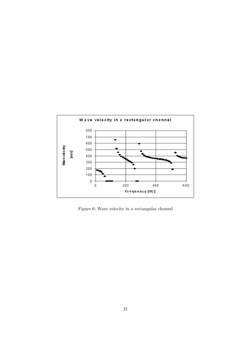
Figure 6: Wave velocity in a rectangular channel

21

4 Unsteady 1D slightly incompressible fluid flow

4.1 Governing equations

Let us start with the 1D incompressible equation of motion and continuity equation:

∂v

∂t+ v

∂v

∂x+

1

ρ

∂p

∂x= S(x, t) where S(x, t) = −g dz

dx− λ

2D|v|v + ax, (58)

∂ρ

∂t+∂ρv

∂x= 0 (59)

Here S(x, t) is the source term, including acceleration due to the inclination of the pipe (g dz/dx),

friction and possible acceleration in the horizontal direction ax.

Let us assume that the fluid is barotropic, i.e. ρ = ρ(p). The continuity equation turns into

∂ρ

∂t+∂ρv

∂x=

dρ

dp︸︷︷︸a−2

∂p

∂t+ ρ

∂v

∂x+ v

dρ

dp

∂p

∂x=

1

a2

(∂p

∂t+ ρa2 ∂v

∂x+ v

∂p

∂x

)= 0, (60)

where a is the sonic velocity. Now we calculate a2(60)+ρa (58):

∂ (p+ ρav)

∂t+ (v + a)

∂ (p+ ρav)

∂x= ρaS(x, t). (61)

Computing a2(60)-ρa(58) gives

∂ (p− ρav)

∂t+ (v − a)

∂ (p− ρav)

∂x= −ρaS(x, t). (62)

Note that the above derivatives are directional derivates:

D+♣Dt

:=∂♣∂t

+ (v + a)∂♣∂x

is a derivative along the linedx

dt= v + a

D−♣Dt

:=∂♣∂t

+ (v − a)∂♣∂x

is a derivative along the linedx

dt= v − a

Hence, by defining α = p+ρav and β = p−ρav, the ordinary differential equations to be solved

are

D+α

Dt= ρaS(x, t) and

D−βDt

= −ρaS(x, t). (63)

4.2 Application on pressurized liquid pipeline systems

In the case of pressurized liquid pipelines (e.g. water distribution systems or oil pipeline systems)

the flow velocity in the pipeline v is typically in the range of a few m/s while the wave velocity a

is in the range of 1000m/s. The bulk modulus of water is B = 2.1GPa, which gives a =√B/ρ =

√2.1× 103 ≈ 1400m/s. Hence the slope of te characetristic lines v ± a is hardly effected by the fluid

velocity. The assumption v a allows the usage of a fix grid as the characteristic slopes are constant:

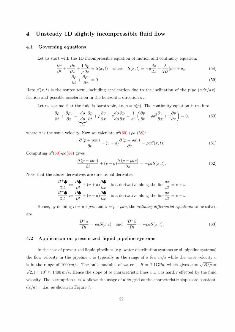
dx/dt = ±a, as shown in Figure 7.

22

4.2.1 Update of the internal points

A simple numerical scheme can be built onto (63), see Figure 7. We use a special grid that

strictly satisfies∆x

∆t= a, (64)

meaning that if e.g. the spatial grid is set, the time step cannot be chosen arbitrarily but must be

computed based on (64). The first step updates the α and β values in the internal points

αi+1j − αij−1

∆t= ρaSij−1 → αi+1

j = αij−1 + ∆tρaSij−1 j = 2 . . . N − 1 (65)

βi+1j − βij+1

∆t= −ρaSij+1 → βi+1

j = βij+1 −∆tρaSij+1 j = 2 . . . N − 1. (66)

Then, we compute pressure and velocity simply by

p =α+ β

2and v =

α− β2ρa

. (67)

Figure 7: Incompressible MOC, numerical scheme.

4.2.2 Boundary conditions

At the boundary points we have only one characteristic equation. For example, on the left

boundary j = 1 based on (66) we have

pi+11 − ρavi+1

1 = pi2ρavi2 −∆tρaSi2 := Kl (68)

Another equation comes from the boundary condition:

Prescribed velocity: vi+11 is known, thus pi+1

1 can be computed based on (68).

23

Prescribed pressure: pi+11 is known, thus vi+1

1 can be computed based on (68).

Prescribed total pressure: pi+11 + ρ

2

(vi+1

1

)2is known and must be solved together with (68).

Pump: the pump performance curve H(Q) is known. We have pi+11 = ps + ρgH(Q), where ps is the

pressure at the suction side of the pump. Furthermore, we have Q = Apvi+11 (Ap is the cross

section area of the pipe), thus the equations to be solved for pi+11 and Q are

pi+11 = ps + ρgH(Q) and pi+1

1 − ρa QAp

= Kl, (69)

which can be rewritten as a single equation for Q:

ps + ρgH(Q)− ρa QAp

= Kl. (70)

TODO Add pump revolution number update here.

The performance curve of a pump H(Q) depends on the revolution number. That is:

pi+11 = ps + ρgH(Q,n). (71)

If n is given, (68) and (71) can be solved for pj+11 and vj+1

1 using e.g. Newton’s technique.

For varying pump revolution number, we need two more pieces of information:

1. H(Q,n)=?

2. How to update nj → nj+1?

1. Affinity lawsQ1

Q2=n1

n2,

H1

H2=

(n1

n2

)2

⇒ p1

p2=

(n1

n2

)3

(72)

Suppose we have

H1(Q) = a0 + a1Q1 + a2Q21 + a3Q

31 + . . . (73)

at revolution number n1. Then by substitution we get

H2

(n1

n2

)2

︸ ︷︷ ︸H1

= a0 + a1

(n

n2

)Q2 + a2

(n1

n2

)2

Q22 + . . . (74)

Thus H(Q,n) can be computed in the following way:

H(Q,n) = a0

(n

n1

)2

+ a1

(n

n1

)Q+ a2Q

2 + a3

(n1

n

)Q3 + . . . (75)

where ai are the fit coefficients of the performance curve at n1.

24

2. Pump revolution number update

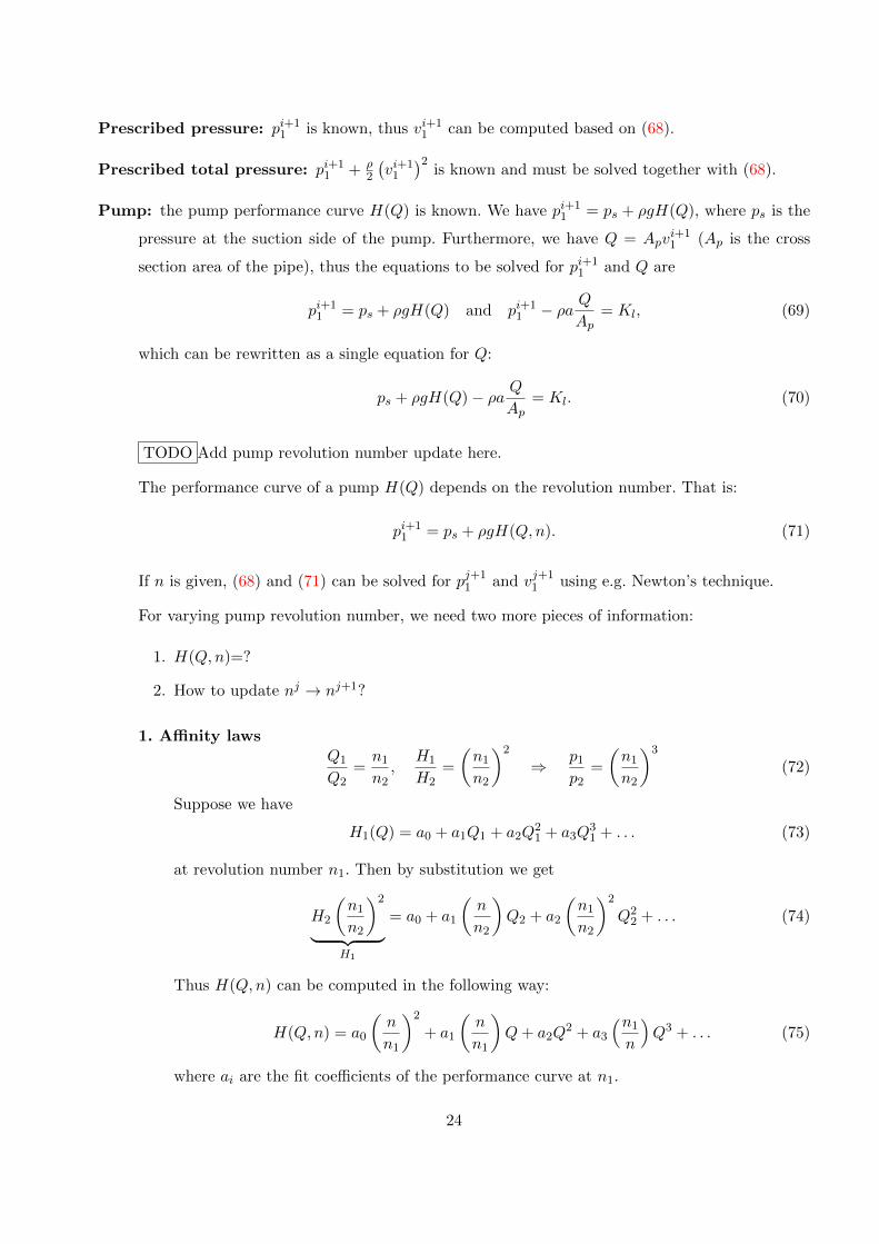
Θ · ε = Melectr. −Mhydraulic (76)

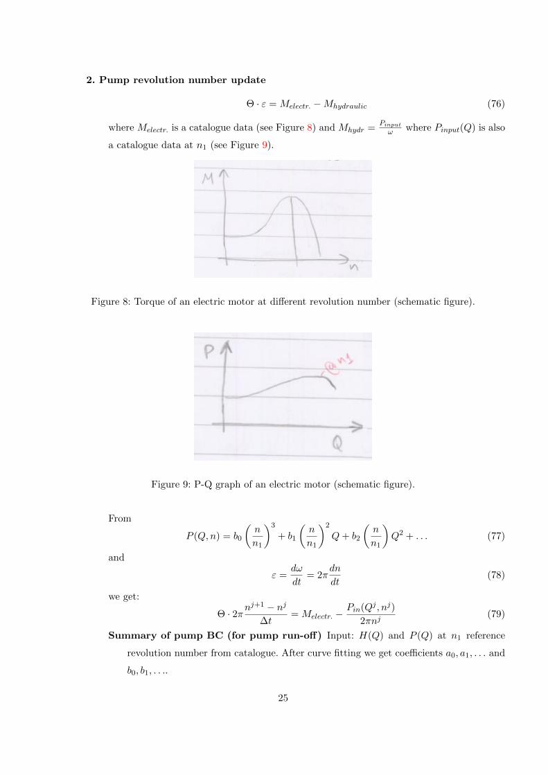
where Melectr. is a catalogue data (see Figure 8) and Mhydr =Pinputω where Pinput(Q) is also

a catalogue data at n1 (see Figure 9).

Figure 8: Torque of an electric motor at different revolution number (schematic figure).

Figure 9: P-Q graph of an electric motor (schematic figure).

From

P (Q,n) = b0

(n

n1

)3

+ b1

(n

n1

)2

Q+ b2

(n

n1

)Q2 + . . . (77)

and

ε =dω

dt= 2π

dn

dt(78)

we get:

Θ · 2πnj+1 − nj

∆t= Melectr. −

Pin(Qj , nj)

2πnj(79)

Summary of pump BC (for pump run-off) Input: H(Q) and P (Q) at n1 reference

revolution number from catalogue. After curve fitting we get coefficients a0, a1, . . . and

b0, b1, . . ..

25

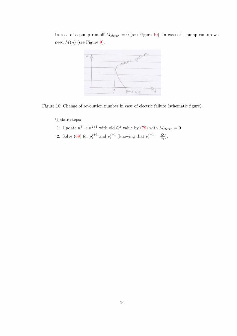
In case of a pump run-off Melectr. = 0 (see Figure 10). In case of a pump run-up we

need M(n) (see Figure 9).

Figure 10: Change of revolution number in case of electric failure (schematic figure).

Update steps:

1. Update nj → nj+1 with old Qj value by (79) with Melectr. = 0

2. Solve (69) for pj+11 and vj+1

1 (knowing that vj+11 = Q

Ap).

26

5 Impedance method

The impedance technique presented in this chapter allows the calculation of hydraulic eigen-

frequencies of pipeline systems. The basic frequency of a pipeline of length L and sonic velocity a is

f = a/(2L), where 2L/a is the time scale of the pipe; i.e. the time needed for a pressure wave to

travel to the other end of the time and come back. However, for more complicated pipelines, it is not

straightforward to cope with the interaction between different pipe segments.

The impedance technique assumes periodic flow in the pipeline and connects the amplitude

of the excitation at one end with the response amplitude on the other end of the pipe, for arbitrary

excitation frequency. Thus with the help of this technique, it is possible to construct resonance diagrams

of complex (tree-like or looped) pipeline systems.

5.1 Basic theory

We start from the one dimensional continuity and momentum equation. The convective terms

are neglected in both equations. We denote the sum of the static pressure pst and hydrostatic pressure

ρgh by p

p = pst + ρgh,

thus the basic equations are:

∂p

∂x+ ρ

∂v

∂t+ρλ

2dv |v| = 0, (80)

1

a2

∂p

∂t+ ρ

∂v

∂x= 0. (81)

We consider only periodic flows. Let the mean values of pressure and velocity be p and v respectively,

and the periodic parts be denoted by p and v:

p = p+ p′; v = v + v′. (82)

The mean values are defined by the time integrals:

p (x) =1

T

∫ T

0p(t, x)dt and v(x) =

1

T

∫ T

0v(t, x)dt. (83)

In order to substitute (82) into (80) and (81) one has to differentiate the pressure and velocity:

∂p

∂x=∂p

∂x+∂p′

∂xand

∂v

∂x=∂v

∂x+∂v′

∂x. (84)

The derivatives with respect to time are similar. By Eq. (83)

∂p

∂t= 0 and

∂v

∂t= 0. (85)

27

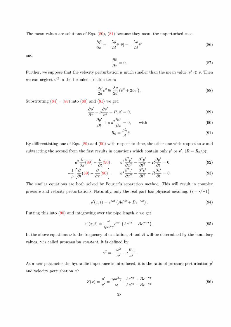
The mean values are solutions of Eqs. (80), (81) because they mean the unperturbed case:

∂p

∂x= −λρ

2dv |v| = −λρ

2dv2 (86)

and∂v

∂x= 0. (87)

Further, we suppose that the velocity perturbation is much smaller than the mean value: v′ v. Then

we can neglect v′2 in the turbulent friction term:

λρ

2dv2 ∼=

λρ

2d

(v2 + 2vv′

). (88)

Substituting (84) – (88) into (80) and (81) we get:

∂p′

∂x+ ρ

∂v′

∂t+R0v

′ = 0, (89)

∂p′

∂t+ ρ a2∂v

′

∂x= 0, with (90)

R0 =ρλ

dv. (91)

By differentiating one of Eqs. (89) and (90) with respect to time, the other one with respect to x and

subtracting the second from the first results in equations which contain only p′ or v′. (R = R0/ρ):

a2 ∂

∂x(89)− ∂

∂t(90) : a2∂

2p′

∂x2− ∂2p′

∂t2−R∂p

′

∂t= 0, (92)

−1

ρ

[∂

∂t(89)− ∂

∂x(90)

]: a2∂

2v′

∂x2− ∂2v′

∂t2−R∂v

′

∂t= 0. (93)

The similar equations are both solved by Fourier’s separation method. This will result in complex

pressure and velocity perturbations: Naturally, only the real part has physical meaning.(ı =√−1)

p′(x, t) = eıωt(Aeγx +Be−γx

). (94)

Putting this into (90) and integrating over the pipe length x we get

v′(x, t) =ω

ıρa2γeıωt

(Aeγx −Be−γx

). (95)

In the above equations ω is the frequency of excitation, A and B will be determined by the boundary

values, γ is called propagation constant. It is defined by

γ2 = −ω2

a2+ ı

Rω

a2.

As a new parameter the hydraulic impedance is introduced, it is the ratio of pressure perturbation p′

and velocity perturbation v′:

Z(x) =p′

v′=ıρa2γ

ω· Ae

γx +Be−γx

Aeγx −Be−γx(96)

28

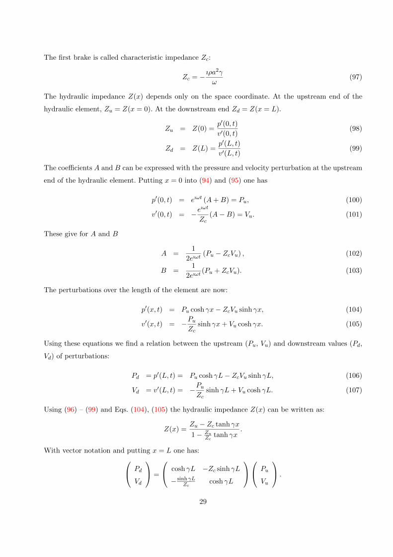
The first brake is called characteristic impedance Zc:

Zc = − ıρa2γ

ω(97)

The hydraulic impedance Z(x) depends only on the space coordinate. At the upstream end of the

hydraulic element, Zu = Z(x = 0). At the downstream end Zd = Z(x = L).

Zu = Z(0) =p′(0, t)

v′(0, t)(98)

Zd = Z(L) =p′(L, t)

v′(L, t)(99)

The coefficients A and B can be expressed with the pressure and velocity perturbation at the upstream

end of the hydraulic element. Putting x = 0 into (94) and (95) one has

p′(0, t) = eıωt (A+B) = Pu, (100)

v′(0, t) = −eıωt

Zc(A−B) = Vu. (101)

These give for A and B

A =1

2eıωt(Pu − ZcVu) , (102)

B =1

2eıωt(Pu + ZcVu). (103)

The perturbations over the length of the element are now:

p′(x, t) = Pu cosh γx− ZcVu sinh γx, (104)

v′(x, t) = −PuZc

sinh γx+ Vu cosh γx. (105)

Using these equations we find a relation between the upstream (Pu, Vu) and downstream values (Pd,

Vd) of perturbations:

Pd = p′(L, t) = Pu cosh γL− ZcVu sinh γL, (106)

Vd = v′(L, t) = −PuZc

sinh γL+ Vu cosh γL. (107)

Using (96) – (99) and Eqs. (104), (105) the hydraulic impedance Z(x) can be written as:

Z(x) =Zu − Zc tanh γx

1− ZuZc

tanh γx.

With vector notation and putting x = L one has: Pd

Vd

=

cosh γL −Zc sinh γL

− sinh γLZc

cosh γL

Pu

Vu

.

29

The matrix is called impedance matrix. The resulting impedance matrix of hydraulic elements con-

nected in series is the product of the impedance matrices of the individual elements. The following

expression connects the impedances at the upstream and downstream ends of the element:

Zd =Zu − Zc tanh γL

1− ZuZc

tanh γL.

5.2 Boundary conditions

Some simple cases are studied where either the upstream or the downstream impedance (Zu

or Zd) can be found easily. The pressure perturbation is zero if the downstream pressure has a fixed

constant value (open end to the atmosphere or a liquid tank with constant surface)

Zd =p′(L, t)

v′(L, t)= 0

Closed end of a pipe, the velocity perturbation is zero, thus

Zd =∞

Dividing or combining pipes (or other hydraulic elements) results in a boundary condition where the

pressure perturbation is common for all connected elements and continuity is fulfilled. For elements k

being connected (k = 1, 2, . . . ,K):

p′1(Li, t) = p′2(L2, t) = . . . = p′k(LK , t) (108)

Supposing constant liquid density in elements having cross sections Ak gives:

K∑k=1

Ak(vk + v′k

)= 0.

Continuity must be fulfilled for the mean velocities v too,

K∑k=1

Akv′k = 0. (109)

From (108) and (109)K∑k=1

AkZk

= 0.

The fact that the velocity is proportional to the square root of pressure difference in turbulent flow is

used to formulate the impedance of a throttle valve at the downstream end of a pipe:

v + v′ = µ

√2

ρ(∆p+ ∆p′).

30

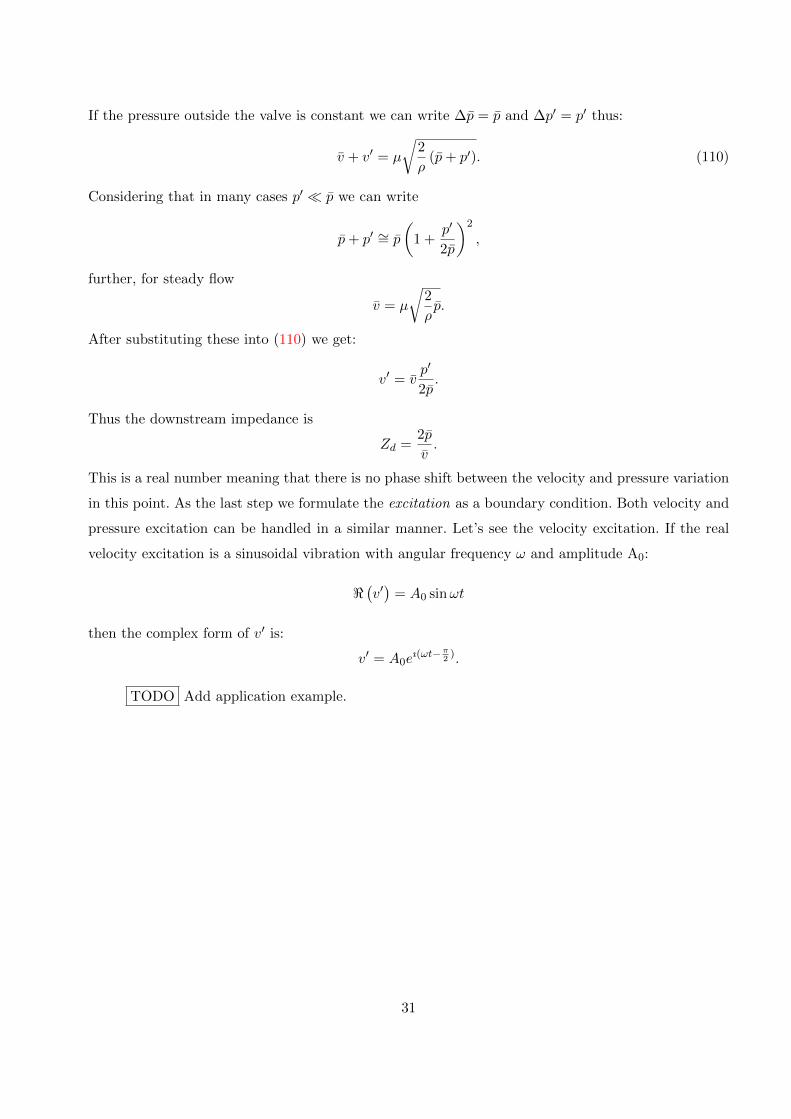
If the pressure outside the valve is constant we can write ∆p = p and ∆p′ = p′ thus:

v + v′ = µ

√2

ρ(p+ p′). (110)

Considering that in many cases p′ p we can write

p+ p′ ∼= p

(1 +

p′

2p

)2

,

further, for steady flow

v = µ

√2

ρp.

After substituting these into (110) we get:

v′ = vp′

2p.

Thus the downstream impedance is

Zd =2p

v.

This is a real number meaning that there is no phase shift between the velocity and pressure variation

in this point. As the last step we formulate the excitation as a boundary condition. Both velocity and

pressure excitation can be handled in a similar manner. Let’s see the velocity excitation. If the real

velocity excitation is a sinusoidal vibration with angular frequency ω and amplitude A0:

<(v′)

= A0 sinωt

then the complex form of v′ is:

v′ = A0eı(ωt−π

2).

TODO Add application example.

31

6 Unsteady 1D open-surface flow in prismatic channel

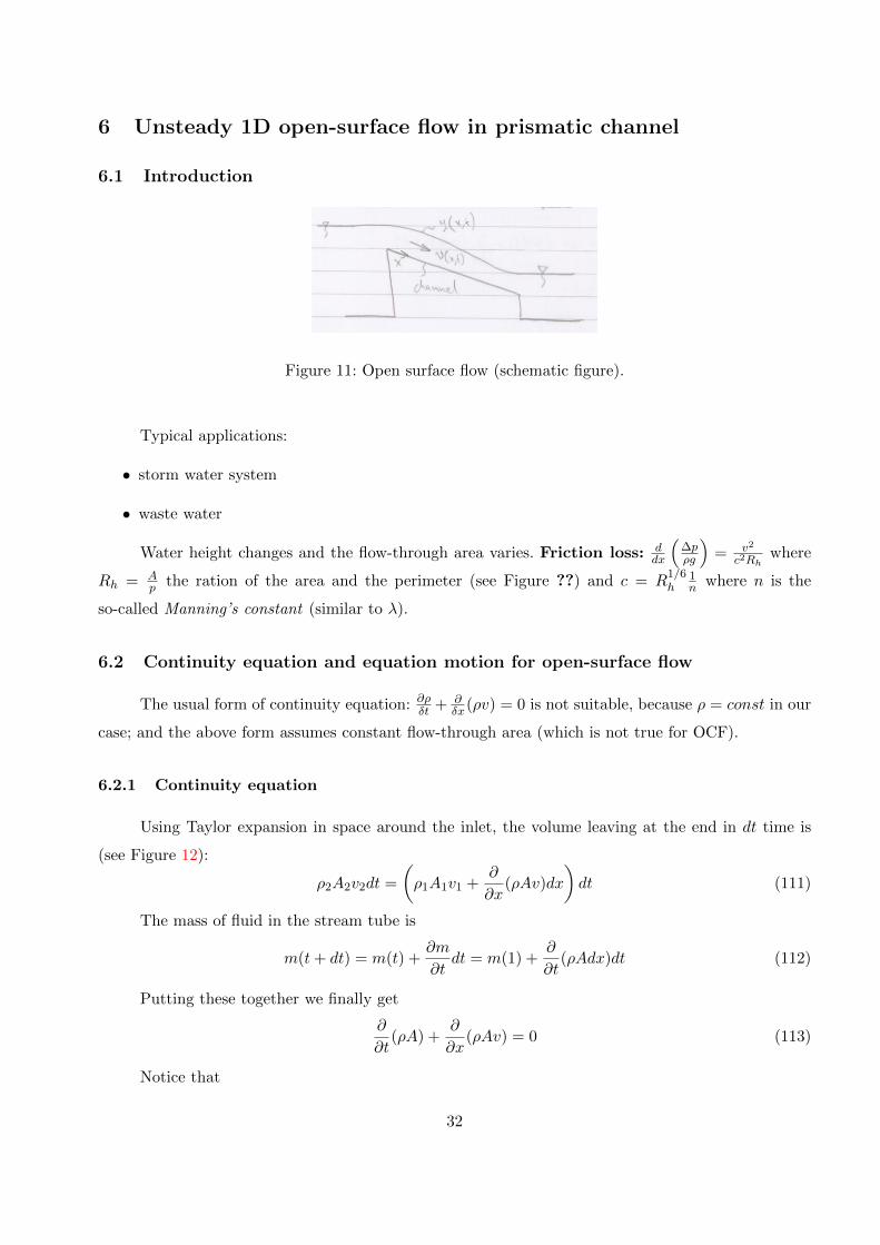
6.1 Introduction

Figure 11: Open surface flow (schematic figure).

Typical applications:

• storm water system

• waste water

Water height changes and the flow-through area varies. Friction loss: ddx

(∆pρg

)= v2

c2Rhwhere

Rh = Ap the ration of the area and the perimeter (see Figure ??) and c = R

1/6h

1n where n is the

so-called Manning’s constant (similar to λ).

6.2 Continuity equation and equation motion for open-surface flow

The usual form of continuity equation: ∂ρδt + ∂δx(ρv) = 0 is not suitable, because ρ = const in our

case; and the above form assumes constant flow-through area (which is not true for OCF).

6.2.1 Continuity equation

Using Taylor expansion in space around the inlet, the volume leaving at the end in dt time is

(see Figure 12):

ρ2A2v2dt =

(ρ1A1v1 +

∂

∂x(ρAv)dx

)dt (111)

The mass of fluid in the stream tube is

m(t+ dt) = m(t) +∂m

∂tdt = m(1) +

∂

∂t(ρAdx)dt (112)

Putting these together we finally get

∂

∂t(ρA) +

∂

∂x(ρAv) = 0 (113)

Notice that

32

• if A = const then get back the usual form: ∂ρ∂t + ∂(ρv)

∂x = 0 and

• if ρ = const then ∂A∂t + ∂Q

∂x = 0 (the volumetric flow rate is Q = Av).

6.2.2 Equation of motion

From Newton’s II. law we know that

dF

dt= Fpressure + Fgravity + Ffriction (114)

Using first order expansion

Figure 12: Open surface flow (schematic figure).

TODO

The general form is

∂ρvA

∂t+∂(vρvA)

∂x= −A

(∂p

∂x− ρgS0 + ρgSf

)(115)

where S0 = −dz/dx is the bed slope and Sf = f2Dgv

2 is the friction loss.

6.2.3 General vector form for open-surface flow

For ρ = 0, the momentum equation can be written as

∂Q

∂t+∂ Qv

∂x= −A

(1

ρ

∂p

∂x− gS0 + gSf

). (116)

Taking into account that p = ρgy and −A1ρ∂p∂x = −

(∂Agy∂x − yg

∂A∂x

), we have

∂Q

∂t+

∂

∂x

(Q2

A+Agy

)= yg

∂A

∂x+ gA (S0 − Sf ) . (117)

33

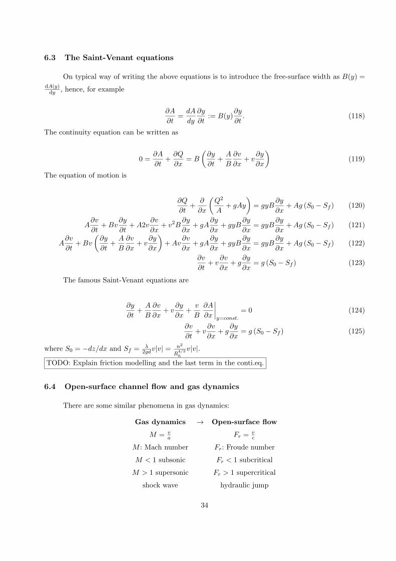
6.3 The Saint-Venant equations

On typical way of writing the above equations is to introduce the free-surface width as B(y) =dA(y)

dy , hence, for example

∂A

∂t=dA

dy

∂y

∂t:= B(y)

∂y

∂t. (118)

The continuity equation can be written as

0 =∂A

∂t+∂Q

∂x= B

(∂y

∂t+A

B

∂v

∂x+ v

∂y

∂x

)(119)

The equation of motion is

∂Q

∂t+

∂

∂x

(Q2

A+ gAy

)= gyB

∂y

∂x+Ag (S0 − Sf ) (120)

A∂v

∂t+Bv

∂y

∂t+A2v

∂v

∂x+ v2B

∂y

∂x+ gA

∂y

∂x+ gyB

∂y

∂x= gyB

∂y

∂x+Ag (S0 − Sf ) (121)

A∂v

∂t+Bv

(∂y

∂t+A

B

∂v

∂x+ v

∂y

∂x

)+Av

∂v

∂x+ gA

∂y

∂x+ gyB

∂y

∂x= gyB

∂y

∂x+Ag (S0 − Sf ) (122)

∂v

∂t+ v

∂v

∂x+ g

∂y

∂x= g (S0 − Sf ) (123)

The famous Saint-Venant equations are

∂y

∂t+A

B

∂v

∂x+ v

∂y

∂x+v

B

∂A

∂x

∣∣∣∣y=const.

= 0 (124)

∂v

∂t+ v

∂v

∂x+ g

∂y

∂x= g (S0 − Sf ) (125)

where S0 = −dz/dx and Sf = λ2gdv|v| =

n2

R4/3h

v|v|.

TODO: Explain friction modelling and the last term in the conti.eq.

6.4 Open-surface channel flow and gas dynamics

There are some similar phenomena in gas dynamics:

Gas dynamics → Open-surface flow

M = va Fr = v

c

M : Mach number Fr: Froude number

M < 1 subsonic Fr < 1 subcritical

M > 1 supersonic Fr > 1 supercritical

shock wave hydraulic jump

34

6.5 Method of characteristics for open-surface flow

6.5.1 MOC formulation for rectangular channel

The Saint-Venant equation can be re-written in terms of wave celerity c =√gy instead of water

depth. First, we compute

∂y

∂t=

1

g

∂c2

∂t=

2c

g

∂c

∂tand

∂y

∂x=

1

g

∂c2

∂x=

2c

g

∂c

∂x. (126)

we have now

2c

g

∂c

∂t+A

B

∂v

∂x+ v

2c

g

∂c

∂x= 0 (127)

∂v

∂t+ v

∂v

∂x+ 2c

∂c

∂x= g (S0 − Sf ) (128)

Upon adding the two equations, i.e. EoM +K × Continuity:

(∂v

∂t+K

2c

g

∂c

∂t

)+ v

(∂v

∂x+K

2c

g

∂c

∂x

)+

(2c∂c

∂x+Ky

∂v

∂x

)= 0. (129)

Upon choosing K = ±gc , we have TODO: Explain the choice of K.

(∂v

∂t± 2

∂c

∂t

)+ v

(∂v

∂x± 2

∂c

∂x

)+ c

(2∂c

∂x± ∂v

∂x

)= g (S0 − Sf ) or, upon rearranging, (130)

∂

∂t(v ± 2c) + (v ± c) ∂

∂x(v ± 2c) = g (S0 − Sf ) . (131)

6.5.2 Numerical technique for the internal points

In the case of open-surface flows, there are several differences between the slightly compressible

case (pressurized pipeline systems):

• c =√gy not constant

• v << c can happen (e.g:y = 1ms → c ≈ 3ms )

• even v > c can happen!

Timestep selection

35

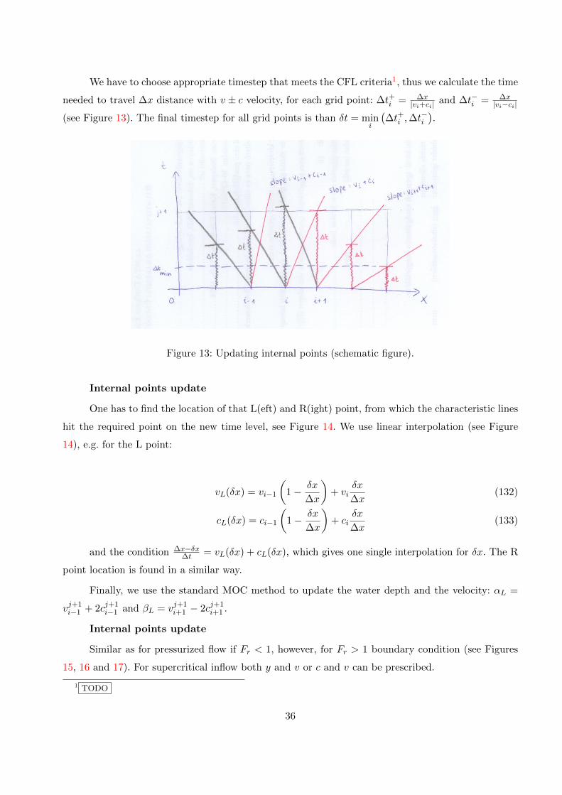
We have to choose appropriate timestep that meets the CFL criteria1, thus we calculate the time

needed to travel ∆x distance with v ± c velocity, for each grid point: ∆t+i = ∆x|vi+ci| and ∆t−i = ∆x

|vi−ci|

(see Figure 13). The final timestep for all grid points is than δt = mini

(∆t+i ,∆t

−i

).

Figure 13: Updating internal points (schematic figure).

Internal points update

One has to find the location of that L(eft) and R(ight) point, from which the characteristic lines

hit the required point on the new time level, see Figure 14. We use linear interpolation (see Figure

14), e.g. for the L point:

vL(δx) = vi−1

(1− δx

∆x

)+ vi

δx

∆x(132)

cL(δx) = ci−1

(1− δx

∆x

)+ ci

δx

∆x(133)

and the condition ∆x−δx∆t = vL(δx) + cL(δx), which gives one single interpolation for δx. The R

point location is found in a similar way.

Finally, we use the standard MOC method to update the water depth and the velocity: αL =

vj+1i−1 + 2cj+1

i−1 and βL = vj+1i+1 − 2cj+1

i+1 .

Internal points update

Similar as for pressurized flow if Fr < 1, however, for Fr > 1 boundary condition (see Figures

15, 16 and 17). For supercritical inflow both y and v or c and v can be prescribed.

1 TODO

36

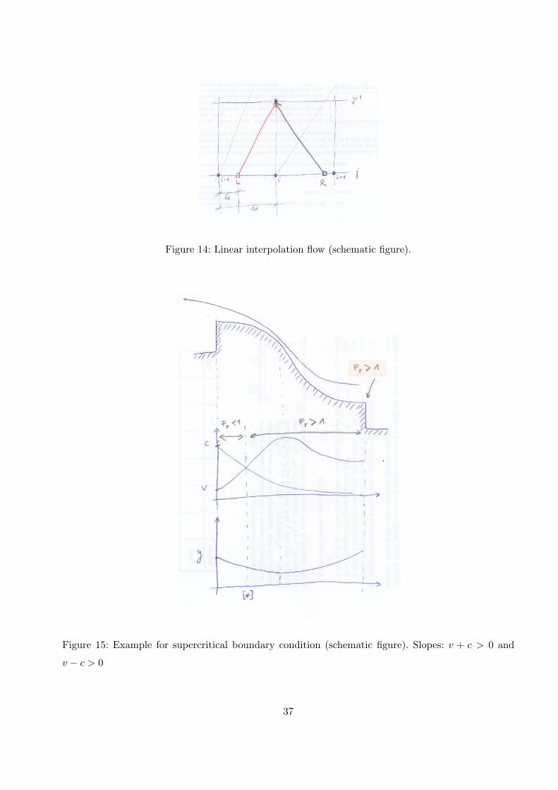
Figure 14: Linear interpolation flow (schematic figure).

Figure 15: Example for supercritical boundary condition (schematic figure). Slopes: v + c > 0 and

v − c > 0

37

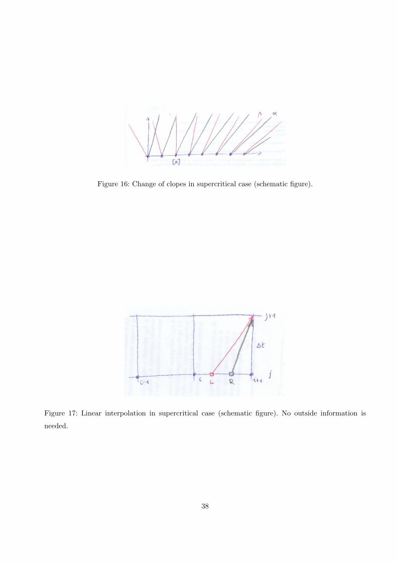
Figure 16: Change of clopes in supercritical case (schematic figure).

Figure 17: Linear interpolation in supercritical case (schematic figure). No outside information is

needed.

38

7 Unsteady 1D compressible gas flow

7.1 Governing equations

Let us start off with the 1D integral form of the continuity equation

∂

∂t

∫VρdV +

∮Aρv dA = 0, (134)

equation of motion∂

∂t

∫VρvdV +

∮Avρv dA = −

∮Ap dA+

∮Aτ dA, (135)

and energy equation∂

∂t

∫VρedV +

∮Aeρv dA = −

∮Apv dA+

∮Aq dA (136)

where τ is the stress tensor, e = u+ v2/2 (for an ideal gas, we have du = cV dT ) is the sum of internal

energy and kinetic energy and q is the heat flux vector. We also need an equation of state of the form

p = f(ρ, u).

In what follows, we assume 1D flow, hence v = v(x, t).

Applying the divergence theorem on the continuity equation and expoiting that V = A(x)x, we

have

∂

∂t

∫VρdV +

∫V

∂

∂x(ρv) dV =

∫ (∂ ρA

∂t+∂ ρvA

∂x

)dx = 0. (137)

∂ ρA

∂t+∂ ρvA

∂x= 0. (138)

The equation of motion takes the form

∂

∂t

∫VρvdV +

∫V

∂

∂xρv2 dV = −

∫∂p

∂xAdx+

∮Aτ dA (139)∫ (

∂

∂tρvA+

∂

∂xAρv2

)dx = −

∫ (∂(pA)

∂x− pdA

dx

)dx+

∫Fs dx (140)

∂

∂tρvA+

∂

∂x

(Aρv2 + pA

)= p

dA

dx+ Fs = Fp + Fs. (141)

The energy equation can be rewritten in a similar way. Finally, the system of equation to be solved

are

∂

∂t(ρA) +

∂

∂x(ρvA) = 0 (142)

∂

∂t(ρvA) +

∂

∂x

(Aρv2 + pA

)= Fp + Fs (143)

∂

∂t(ρeA) +

∂

∂x(Aρve+ pvA) = Q (144)

39

7.2 Isentropic MOC

Let us start off with some basic equations from thermodynamics. From the ideal gas law and

the isentropic process, we have

ρ

ρ0=

(T

T0

) 1κ−1

=

(a

a0

) 2κ−1

, (145)

∂ρ

∂x= ρ0

2

κ− 1

(a

a0

) 2κ−1−1 ∂a

∂x

1

a0= ρ0

2

κ− 1

ρ

ρ0

(a

a0

)−1 ∂a

∂x

1

a0=

2

κ− 1

ρ

a

∂a

∂x, (146)

∂ρ

∂t=

2

κ− 1

ρ

a

∂a

∂tand (147)

a2 =∂p

∂ρ

∣∣∣∣isentropic

→ ∂p

∂x= a2∂ρ

∂t. (148)

Now, the continuity equation is

∂ρ

∂t+∂(ρv)

∂x=

2

κ− 1

ρ

a

∂a

∂t+ v

2

κ− 1

ρ

a

∂a

∂x︸ ︷︷ ︸v ∂ρ∂x

+ρ∂v

∂x(149)

=2

κ− 1

ρ

a

(∂a

∂t+ v

∂a

∂x

)+ ρ

∂v

∂x=

2

κ− 1

ρ

a

da

dt+ ρ

∂v

∂x= 0 (150)

and the equation of motion becomes

∂v

∂t+ v

∂v

∂x+

1

ρ

∂p

∂x=

dv

dt+ a

2

κ− 1

∂a

∂t= 0 (151)

Computing aρκ−1

2 (150) +κ−12 (151) gives

0 =da

dt+κ− 1

2a∂v

∂x+κ− 1

2

dv

dt+ a

∂a

∂t=

(da

dt+ a

∂a

∂x

)+κ− 1

2

(dv

dt+ a

∂v

∂x

)(152)

=

(∂a

∂t+ (a+ v)

∂a

∂x

)+κ− 1

2

(∂v

∂t+ (a+ v)

∂v

∂x

)(153)

:=D+a

D+t+κ− 1

2

D+v

D+t=D+

D+t

(a+

κ− 1

2v

):=D+α

D+t(154)

A similar computation with aρκ−1

2 (150) −κ−12 (151) gives

0 =D−βD−t

withD−

D−t=

∂

∂t+ (v − a)

∂

∂xand β = a− κ− 1

2v (155)

40

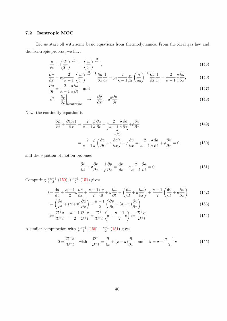
7.3 Boundary conditions

In what follows we give all the equations for the beginning of the domain, i.e. the first node with

subscript 1.

Figure 18: Boundary conditions in the case of subsonic flow.

7.3.1 Subsonic, isentropic inflow

The ambient gas properties (far away from the inlet) are p0, T0 and ρ0. We are searching for T1,

a1, v1 and ρ1. We have

• Characteristics from the inside of the pipe: βR = a1 − κ−12 v1 with βR being known.

• Constant total temperature from the surroundings: T0 = T1 +v212cp

= a2

κR +v212cp

.

These two equations can be solved for a1 and v1.

7.3.2 Supersonic, isentropic inflow

The ambient gas properties (far away from the inlet) are p0, T0 and ρ0. We are searching for T1,

a1, v1 and ρ1. We have

• Characteristics from the inside of the pipe cannot be used as it is vertical.

• The velocity is v1 = a1.

• The inflow is still isentropic: T0 = T1 +v212cp

=a21κR +

a212cp

.

41

7.3.3 Subsonic, isentropic outflow

The ambient gas properties (far away from the inlet) are p0, T0 and ρ0. We are searching for T1,

a1, v1 and ρ1. We have

• Characteristics from the inside of the pipe: βR = a1 − κ−12 v1 with βR being known.

• The pressure change is isentropic: a1aR

=(p1pR

)κ−12κ

.

• The pressure at the outlet is p0 = p1.

7.3.4 Supersonic, isentropic outflow

• We have v1 = −a1

• Characteristics from the inside of the pipe: βR = a1 − κ−12 v1 with βR being known.

• We also have: αL = a1 + κ−12 v1 with αL being known.

• The inflow is still isentropic: T0 = T1 +v212cp

=a21κR +

a212cp

.

7.3.5 How do we decide if we have inflow or outflow?

At x = 0, for inflow, we have

2a0 > 2a1 = α1 + β1 and (156)

α1 − β1 = (κ− 1) v1 > 0 (157)

After adding these two equations, we obtain β1 > a0 as a condition for inflow .

42

7.4 The Lax-Wendroff scheme

The governing equations can be written in a compact form

∂U∂t

+∂F∂x

= Q, (158)

with

U =

ρA

ρvA

ρeA

, F =

ρvA(

ρv2 + p)A

(ρev + pv)A

, and U =

0

Fp + Fs

Q

. (159)

Here the internal energy e = cV T , Fp = pdA(x)dx and Fs = Aρ

2λDv|v|.

Note that if U is known, the primitive valiables can also be computed: ρ = U1/A, v = U2/U1

and e = U3/U1.

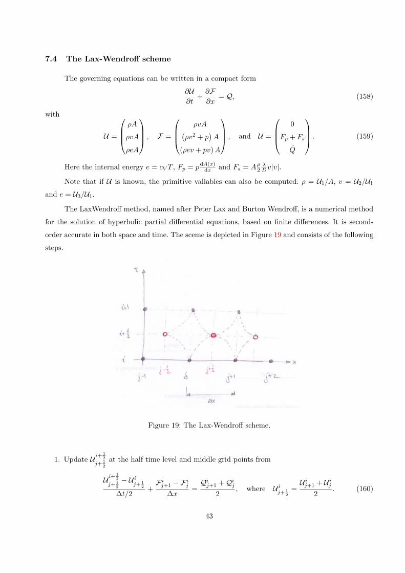
The LaxWendroff method, named after Peter Lax and Burton Wendroff, is a numerical method

for the solution of hyperbolic partial differential equations, based on finite differences. It is second-

order accurate in both space and time. The sceme is depicted in Figure 19 and consists of the following

steps.

Figure 19: The Lax-Wendroff scheme.

1. Update U i+12

j+ 12

at the half time level and middle grid points from

U i+12

j+ 12

− U ij+ 1

2

∆t/2+F ij+1 −F ij

∆x=Qij+1 +Qij

2, where U i

j+ 12

=U ij+1 + U ij

2. (160)

43

2. ’Unpack’ the primitive valiables and compute F i+12

j+ 12

.

3. Take a full time step to compute U i+1j with the help of F i+

12

j+ 12

:

U i+1j − U ij

∆t+F i+

12

j+ 12

−F i+12

j− 12

∆x=Qi+

12

j+ 12

+Qi+12

j− 12

2. (161)

The time step ∆t cannot be chosen arbitrarily, the timestep should be small enough to ensure

that the scheme does not ’steps over’ a cell with information propagation velocity a+ |v|:

∆tj < C∆x

aj + |vj |, ∆t = min ∆tj , (162)

where C < 1 is the ’safety’ factor and aj =√κRTj .

44

8 General framework on characteristic lines of PDEs

The equation of continuity – considering barotropic fluid

∂p

∂t+ v

∂p

∂x+ ρa2 ∂v

∂x= 0, (163)

and the equation of motion∂v

∂t+ v

∂v

∂x+

1

ρ

∂p

∂x= S(x, t) (164)

describe the 1D unsteady flow of a slightly compressible fluid c1where p is the pressure, v is the veloc- c1Viktor: Textadded.

ity, S is the friction and a is the wave velocity. We neglect the source term S. Let’s find the solution

of the above system of first order partial differential equations in the form of

p = peı(kx−ωt), v = veı(kx−ωt). (165)

Substituting the derivatives into the above equations and dropping the non-zero term ıeı(kx−ωt) we

get

− ωp+ kvp+ ρa2kv = 0, and − ωv +1

ρkp+ kvv = 0 respectively (166)

which is a linear homogeneous system of algebraic equations for the amplitudes p, v. Only the trivial

solution (p = 0, v = 0) exists if the determinant of the coefficient matrix is non-zero. Thus the

determinant must be zero: ∣∣∣∣∣∣ −ω + kv ρa2k

kρ −ω + kv

∣∣∣∣∣∣ = 0, (167)

that is (−ω + kv)2 − a2k2 = 0, or −ω + kv = ±ak, which after rearranging reads ω = k(v ± a).

Substituting this into p(x, t) and v(x, t), we get:

p(x, t) = peık[x−(v±a)t], v(x, t) = veık[x−(v±a)t]. (168)

Thus if the source term S is zero the value of p and v does not change along the lines:

x− (v ± a)t = const., (169)

these are the so-called characteristics. Physically this means that the shape of the pressure or velocity

distribution along the pipe at some time t is kept but it is shifted to some other location determined

by (169). This is typical for the propagation of wave forms.

8.1 Solution of general partial differential equations describing fluid flow

After having seen that the system of flow equations

∂p

∂t+ v

∂p

∂x+ ρa2 ∂v

∂x= 0 and (170)

∂v

∂t+ v

∂v

∂x+

1

ρ

∂p

∂x= S(x, t) (171)

45

describe the propagation of pressure (and fluid speed) waves we try to formulate the PDE of a pressure

wave. Differentiating (170) with respect to t:

∂2p

∂t2+∂v

∂t

∂p

∂x+ v

∂2p

∂x∂t+ ρa2 ∂

2v

∂x∂t= 0. (172)

Differentiating (171) with respect to x:

∂2v

∂t∂x+

(∂v

∂x

)2

+ v∂2v

∂x2+

1

ρ

∂2p

∂x2=∂S

∂x. (173)

After substitution

∂2p

∂t2+∂v

∂t

∂p

∂x+ v

∂2p

∂x∂t+ ρa2

(−v ∂

2v

∂x2− 1

ρ

∂2p

∂x2

)= ρa2

(∂v

∂x

)2

− ρa2∂S

∂x. (174)

Besides the derivatives of p the second derivative of the term (v2/2) occurs too. This can be eliminated

by differentiating (170) with respect to x:

ρa2 ∂2v

∂x2= − ∂2p

∂t∂x− ∂v

∂x

∂p

∂x− v ∂

2p

∂x2. (175)

Finally substituting this gives

∂2p

∂t2+ v

∂2p

∂x∂t− a2 ∂

2p

∂x2+ v

∂2p

∂x∂t+ v2 ∂

2p

∂x2= −ρa2∂S

∂x− ∂v

∂t

∂p

∂x+ ρa2

(∂v

∂x

)2

− v ∂v∂x

∂p

∂x. (176)

There are second derivatives of the pressure on the left hand side while all terms on the r.h.s. are of

minor order. Thus the structure of our equation is:

(v2 − a2)∂2p

∂x2+ 2v

∂2p

∂x∂t+∂2p

∂t2= F

(t, x, v,

∂v

∂t,∂v

∂x,∂p

∂x

). (177)

Supposing that the velocity function v(x, t) is known, one has a PDE of 2nd order which is linear in

its higher order terms for the function p(x, t).

8.2 Classification of second order linear PDEs with constant coefficients. Canon-ical form and characteristic differential equation of 2nd order PDE-s.

Following notations are introduced:

x =

x1

x2

; u = u(x); u′ =

∂u∂x1∂u∂x2

. (178)

The second order differential operator L has the form:

Lu =

2∑i=1

2∑k=1

aik (x)∂2u

∂xi∂xk+ f

(x, u,u′

)=

a11 (x)∂2u

∂x21

+ a12 (x)∂2u

∂x1∂x2+ a21 (x)

∂2u

∂x2∂x1+ a22 (x)

∂2u

∂x22

+ f(x, u,u′

). (179)

46

The coefficients are continuous and symmetric that is aik (x) = aki (x) thus

Lu = a11 (x)∂2u

∂x21

+ 2a12 (x)∂2u

∂x1∂x2+ a22 (x)

∂2u

∂x22

+ f(x, u,u′

). (180)

The first part of this operator containing second order derivatives is called the main part. L is a linear

operator since it is linear in the unknown function u.

Definition. The differential operator L in point x is elliptic, hyperbolic or parabolic if the matrixA(x) composed by the coefficients aik(x) in point x is definite, indefinite or semi-definite.

The 2x2 matrix A in any point x has two eigenvalues: λ1 and λ2. We distinguish three different

cases:

• λ1,2 > 0 or λ1,2 < 0 =⇒ L is elliptic

• λ1 > 0 and λ2 < 0 (A is indefinite) =⇒ L is hyperbolic

• λ1 > 0 or λ1 < 0 and λ2 = 0 =⇒ L is parabolic

The PDE itself is called elliptic, hyperbolic or parabolic if L is elliptic, hyperbolic or parabolic. After

this introduction we consider the second order linear PDE (180). Its second order main part is – with

some different notation:

Lu = a (x, y)∂2u

∂x2+ 2b (x, y)

∂2u

∂x∂y+ c (x, y)

∂2u

∂y2. . . (181)

In order to determine the type of the PDE we must find the eigenvalues of

A =

a (x, y) b (x, y)

b (x, y) c (x, y)

. (182)

From

det (A− λE) =

∣∣∣∣∣∣ a (x, y)− λ b (x, y)

b (x, y) c (x, y)− λ

∣∣∣∣∣∣ =

= λ2 − [a (x, y) + c (x, y)]λ+ a (x, y) c (x, y)− b2 (x, y) = λ2 − λ tr (A) + det (A) = 0. (183)

We can now find the eigenvalues by solving this quadratic algebraic equation. We omit the arguments

of the coefficients:

λ1,2 =tr (A)±

√tr2 (A)− 4 det (A)

2=

tr (A)±√

(a+ c)2 − 4 (ac− b2)

2=

=tr (A)±

√(a− c)2 + 4b2

2. (184)

47

We see that the eigenvalues are always real as under the square root the argument is always positive;

this is the corollary of A being symmetric. We denote the determinant by d (x, y) = a (x, y) c (x, y)−

b2 (x, y). The equation (183) has two roots, λ1 and λ2, thus the equation can be written in the form

(λ− λ1) (λ− λ2) = λ2 − λ (λ1 + λ2) + λ1λ2 = 0.

By comparing this with (183) we have

λ1 + λ2 = tr (A) ; λ1λ2 = det (A) = d (x, y) .

The 3 different cases are:

• d(x, y) = 0 =⇒ λ1 = 0 and λ2 = tr(A), thus the PDE is parabolic

• d(x, y) > 0 =⇒ both eigenvalues are either positive or negative, thus the PDE is elliptic

• d(x, y) < 0 =⇒ λ1 > 0 and λ2 < 0, thus the PDE is hyperbolic

From now on we shall only consider the hyperbolic case. In a one dimensional pipe flow the 2nd

order PDE for the pressure is

(v2 − a2)∂2p

∂x2+ 2v

∂2p

∂x∂t+∂2p

∂t2= F

(t, x, v,

∂v

∂t,∂v

∂x,∂p

∂x

). (185)

Here the former space coordinate y is denoted with t, that stands for time. Comparing this equation

with the differential operator L we have

a (x, t) = v2 − a2; b (x, t) = v; c (x, t) = 1,

thus det (A) = d (x, t) = v2 − a2 − v2 = −a2 < 0; L is hyperbolic.

tr (A) = v2 − a2 + 1, λ1,2 =v2 − a2 + 1±

√(v2 − a2 − 1)2 + 4v2

2.

8.3 Coordinate transformation resulting in a simpler form of operator L

Next we transform the independent variables x, t trough the functions ξ = ξ(x, t), η = η(x, t)

resulting in a more simple structure of the left hand side of (185). Let the transformation functions

be continuously differentiable. By the chain rule:

∂

∂x=

∂

∂ξξx +

∂

∂ηηx;

∂

∂t=

∂

∂ξξt +

∂

∂ηηt,

further∂2

∂x2=

(∂2

∂ξ2ξx +

∂2

∂ξ∂ηηx

)ξx +

∂

∂ξξxx +

(∂2

∂η∂ξξx +

∂2

∂η2ηx

)ηx +

∂

∂ηηxx =

48

=∂2

∂ξ2ξ2x + 2

∂2

∂ξ∂ηξxηx +

∂2

∂η2η2x + ξxx

∂

∂ξ+ ηxx

∂

∂η.

Similarly∂2

∂x∂t=

∂2

∂ξ2ξxξt +

∂2

∂ξ∂η(ξxηt + ηxξt) +

∂2

∂η2ηxηt + . . . ,

and∂2

∂t2=

∂2

∂ξ2ξ2t + 2

∂2

∂ξ∂ηξtηt +

∂2

∂η2η2t + . . .

Substituting all these derivatives into the l.h.s. of (185) c1(without p) we have c1Viktor: Textadded.(

(v2 − a2)ξ2x + 2vξxξt + ξ2

t

) ∂2

∂ξ2+ 2

((v2 − a2)ξxηx + v (ξxηt + ηxξt) + ξtηt

) ∂2

∂ξ∂η+

+((v2 − a2)η2

x + 2vηxηt + η2t

) ∂2

∂η2= . . . . (186)

The first and third term have the same structure with the only difference that the first term contains

the derivatives of ξ, while the third term is related to η. The above expression will be simpler if the

1st and 3rd term is set to zero:

(v2 − a2)ξ2x + 2vξxξt + ξ2

t = 0, (v2 − a2)η2x + 2vηxηt + η2

t = 0.

From the first equation

ξt =−2vξx ±

√4v2ξ2

x − 4(v2 − a2)ξ2x

2= (−v ± a)ξx = −(v ± a)ξx.

This is the equation of a ξ(x, t) = const. line as the total difference of ξ is zero along such a line:

dξ = ξxdx+ ξtdt = 0, that is ξt = −dxdtξx.

By comparing the two formulae for ξt one has

dx

dt= v ± a (187)

and ξ(x, t) is constant on the pair of lines defined by (187). Because of the formal similarity the

function η(x, t) is constant too. Equation (187) is called the characteristic differential equation of a

PDE of 2nd order which is linear in its higher order terms. In the present case the solutions of the two

characteristic differential equations are two real characteristics:

x = (v − a)t+ constant,

x = (v + a)t+ constant,

that is

ξ = x− (v − a)t

49

and

η = x− (v + a)t.

The members of the two families of characteristics are ξ = const. and η = const. lines. The ξ = const.

and η = const. lines span a net on the total x,t plane. An appropriate pair of values ξ,η can be attached

to each point of this plane. This attachment is only unique if the different ξ lines do not intersect each

other and the same holds for the different η lines. As the wave velocity a e.g. for acoustic waves is

a =√κRT =

√κp/ρ, thus if the pressure is changing during thee c2the propagation of the pressurec2Viktor: Text

added.wave then the wave velocity may change too. For open surface flows the wave may get steeper as the

wave velocity is higher at the top of a wave than at its bottom. This leads finally to vertical wave

fronts or to water jumps. In gas dynamics the analogous phenomenon is called shock wave. These

discontinuities are excluded from our further investigations. After having found the transformation

resulting in a simpler form of the main part of the differential equation we shall calculate this new

form of the main part. The coefficient of the derivative ∂2p∂ξ∂η in Eq. (186) is −4a2, thus the main part

is

−4a2 ∂2p

∂ξ∂η= . . . .

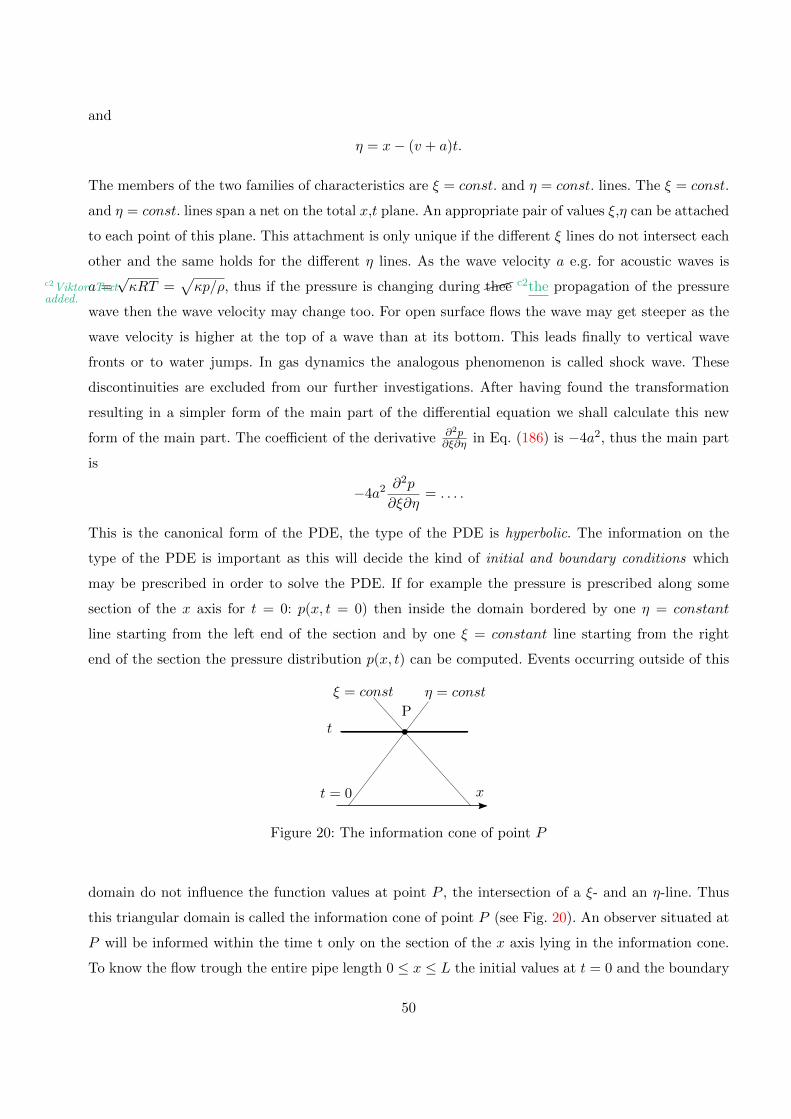
This is the canonical form of the PDE, the type of the PDE is hyperbolic. The information on the

type of the PDE is important as this will decide the kind of initial and boundary conditions which

may be prescribed in order to solve the PDE. If for example the pressure is prescribed along some

section of the x axis for t = 0: p(x, t = 0) then inside the domain bordered by one η = constant

line starting from the left end of the section and by one ξ = constant line starting from the right

end of the section the pressure distribution p(x, t) can be computed. Events occurring outside of this

t

ξ = const η = const

t = 0 x

P

Figure 20: The information cone of point P

domain do not influence the function values at point P , the intersection of a ξ- and an η-line. Thus

this triangular domain is called the information cone of point P (see Fig. 20). An observer situated at

P will be informed within the time t only on the section of the x axis lying in the information cone.

To know the flow trough the entire pipe length 0 ≤ x ≤ L the initial values at t = 0 and the boundary

50

values at x = 0 and at x = L must be known:

p(x = 0, t) and p(x = L, t).

Naturally the boundary values of v(x, t) or some relation between pressure and velocity p(v) is appro-

priate too.

9 Steady 2D supersonic gas flow (in the diffuser part of a Lavalnozzle)

The flow is completely described by the Euler equation and the continuity equation.

1st Euler: u∂u

∂x+ v

∂u

∂y= −1

ρ

∂p

∂x= −1

ρ

dp

dρ

∂ρ

∂x= −a

2

ρ

∂ρ

∂x

∣∣· (− ua2

)(188)

2nd Euler: u∂v

∂x+ v

∂v

∂y= −1

ρ

∂p

∂y= −1

ρ

dp

dρ

∂ρ

∂y= −a

2

ρ

∂ρ

∂y

∣∣· (− va2

)(189)

By multiplying with the given terms and adding these equations we get

− u2

a2

∂u

∂x− uv

a2

∂u

∂y− uv

a2

∂v

∂x− v2

a2

∂v

∂y=u

ρ

∂ρ

∂x+v

ρ

∂ρ

∂y. (190)

Continuity:∂ (ρu)

∂x+∂ (ρv)

∂y= 0 = ρ

(∂u

∂x+∂v

∂y

)+ u

∂ρ

∂x+ v

∂ρ

∂y|: ρ (191)

If we divide by ρ we get the right hand side sum of Eq. (190): uρ∂ρ∂x + v

ρ∂ρ∂y = −

(∂u∂x + ∂v

∂y

). Substituting

this into Eq. (190) the equation of motion has been derived for the supersonic flow:

− u2

a2∂u∂x− uv

a2

(∂u

∂y+∂v

∂x

)− v2

a2

∂v

∂y+∂u

∂x+∂v

∂y=(

1− u2

a2

)∂u

∂x+

(1− v2

a2

)∂v

∂y− uv

a2

(∂u

∂y+∂v

∂x

)= 0. (192)

Assuming isentropic flow the flow is rotation free too. There exists a velocity potential Φ(x, y). The

velocity components u and v can be derived as derivatives of the potential: u = ∂Φ∂x = Φx, v = ∂Φ

∂y = Φy.

We put these and the second order derivatives into Eq. (192):(1− Φ2

x

a2

)Φxx +

(1−

Φ2y

a2

)Φyy − 2

ΦxΦy

a2Φyx = 0. (193)

One can prove that this is a 2nd order PDE of hyperbolic type. We introduce new independent variables

ξ, η instead of x and y. Before we do it we must find an equation for the sonic velocity a too. In steady

isentropic flow the energy equation is htotal = constant. The total enthalpy is:

htotal = h+w2

2= cpT +

w2

2=κRT

κ− 1+w2

2=

a2

κ− 1+w2

2=

1

κ− 1

(a2 + w2κ− 1

2

)= constant (194)

51

The Laval nozzle takes the air from the free atmosphere where the fluid velocity w is zero and the

sonic speed a0 is known. Thus a2 + w2 κ−12 = a2

0 or by rearranging

a2 = a20 − w2κ− 1

2. (195)

Now the transformation of Eq. (193) must be done. In the same way as in Chapter ?? we differentiate

Φ with respect to x(ξ, η) and y(ξ, η) as many times as needed.((1− u2

a2

)ξ2x +

(1− v2

a2

)ξ2y −

2uv

a2ξxξy

)∂2Φ

∂ξ2+ (. . .)

∂2Φ

∂ξ∂η+ (. . .)

∂2Φ

∂η2+ . . . = 0. (196)

In order to simplify this equation the first and third bracketed term must be zero, they have identical

structure. The first term to be made zero us a quadratic equation for ξx. Solving for this we have:

ξx =

2uva2±√

4u2v2

a4ξ2y − 4

(1− u2

a2

)(1− u2

a2

)ξ2y

2(

1− u2

a2

) =

uva2±√

u2+v2

a2− 1

1− u2

a2

ξy. (197)

On the other hand if we consider the ξ = constant line of the new coordinate system, then its total

differential is zero: dξ = ξxdx+ ξydy = 0 which means that dydx = − ξx

ξy. From Eq. (197) the tangent of

the ξ = constant characteristic line is:

dy

dx= −

uva2±√

u2+v2

a2− 1

1− u2

a2

. (198)

One sign is for ξ = constant, the other one for η = constant. Instead of the velocity components u

and v we can introduce the components of the velocity vector w (u = w cosϑ, v = w sinϑ), further

the Mach number: M2 = w2

a2= u2+v2

a2. Then the tangents read

dy

dx= −M

2 sinϑ cosϑ±√M2 − 1

1−M2 cos2 ϑ.

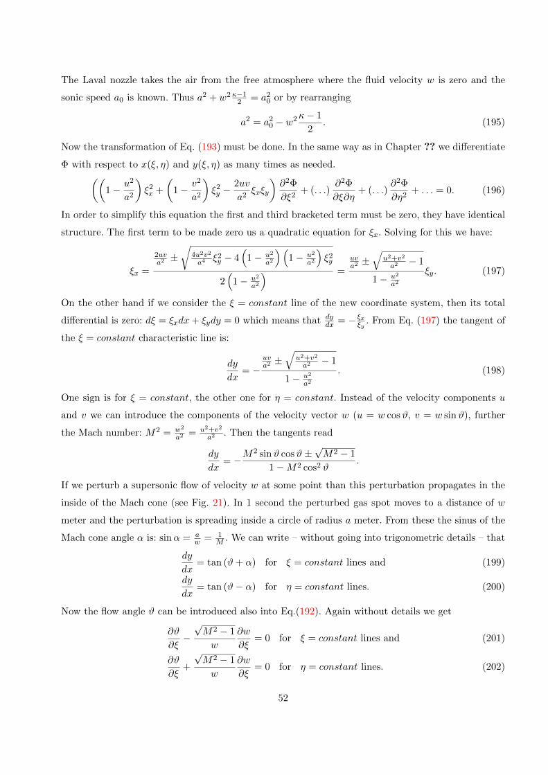
If we perturb a supersonic flow of velocity w at some point than this perturbation propagates in the

inside of the Mach cone (see Fig. 21). In 1 second the perturbed gas spot moves to a distance of w

meter and the perturbation is spreading inside a circle of radius a meter. From these the sinus of the

Mach cone angle α is: sinα = aw = 1

M . We can write – without going into trigonometric details – that

dy

dx= tan (ϑ+ α) for ξ = constant lines and (199)

dy

dx= tan (ϑ− α) for η = constant lines. (200)

Now the flow angle ϑ can be introduced also into Eq.(192). Again without details we get

∂ϑ

∂ξ−√M2 − 1

w

∂w

∂ξ= 0 for ξ = constant lines and (201)

∂ϑ

∂ξ+

√M2 − 1

w

∂w

∂ξ= 0 for η = constant lines. (202)

52

wα

a

Figure 21: Mach cone

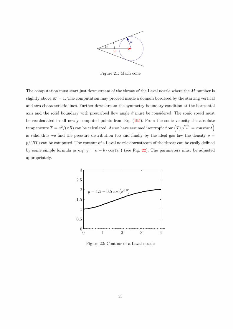
The computation must start just downstream of the throat of the Laval nozzle where the M number is

slightly above M = 1. The computation may proceed inside a domain bordered by the starting vertical

and two characteristic lines. Further downstream the symmetry boundary condition at the horizontal

axis and the solid boundary with prescribed flow angle ϑ must be considered. The sonic speed must

be recalculated in all newly computed points from Eq. (195). From the sonic velocity the absolute

temperature T = a2/(κR) can be calculated. As we have assumed isentropic flow(T/p

κ−1κ = constant

)is valid thus we find the pressure distribution too and finally by the ideal gas law the density ρ =

p/(RT ) can be computed. The contour of a Laval nozzle downstream of the throat can be easily defined

by some simple formula as e.g. y = a − b · cos (xc) (see Fig. 22). The parameters must be adjusted

appropriately.

0 1 2 3 40

0.5

1

1.5

2

2.5

3

y = 1.5− 0.5 cos(x0.8

)

Figure 22: Contour of a Laval nozzle

53