Unravelling the Turing bifurcation using spatially varying ... · Unravelling the Turing...

J. Math. Biol. (1998) 37: 381—417

Unravelling the Turing bifurcation using spatiallyvarying diffusion coefficients

Debbie L. Benson1,2, Philip K. Maini1,w, Jonathan A. Sherratt3

1Centre for Mathematical Biology, Mathematical Institute, 24-29 St Giles’, OxfordOX1 3LB, UK. e-mail: [email protected] College, Oxford, OX1 4AU, UK3Department of Mathematics, Heriot-Watt University, Edinburgh EH14 4AS, UK.e-mail: J.A. [email protected]

Received: 10 January 1996/Revised version: 3 July 1996

Abstract. The Turing bifurcation is the basic bifurcation generatingspatial pattern, and lies at the heart of almost all mathematical modelsfor patterning in biology and chemistry. In this paper the authorsdetermine the structure of this bifurcation for two coupled reactiondiffusion equations on a two-dimensional square spatial domain whenthe diffusion coefficients have a small explicit variation in space acrossthe domain. In the case of homogeneous diffusivities, the Turingbifurcation is highly degenerate. Using a two variable perturbationmethod, the authors show that the small explicit spatial inhomogeneitysplits the bifurcation into two separate primary and two separatesecondary bifurcations, with all solution branches distinct. This split-ting of the bifurcation is more effective than that given by making thedomain slightly rectangular, and shows clearly the structure of theTuring bifurcation and the way in which the various solution branchescollapse together as the spatial variation is reduced. The authorsdetermine the stability of the solution branches, which indicates thatseveral new phenomena are introduced by the spatial variation, includ-ing stable subcritical striped patterns, and the possibility that stablestripes lose stability supercritically to give stable spotted patterns.

Key words: Turing bifurcation — Reaction diffusion — Weakly non-linear — Pattern formation

w Author for correspondence

1 Introduction

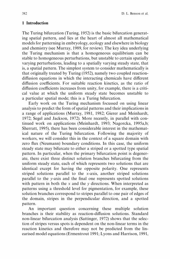
The Turing bifurcation (Turing, 1952) is the basic bifurcation generat-ing spatial pattern, and lies at the heart of almost all mathematicalmodels for patterning in embryology, ecology and elsewhere in biologyand chemistry (see Murray, 1989, for review). The key idea underlyingthe Turing mechanism is that a homogeneous equilibrium can bestable to homogeneous perturbations, but unstable to certain spatiallyvarying perturbations, leading to a spatially varying steady state, thatis, a spatial pattern. The simplest system to consider mathematically isthat originally treated by Turing (1952), namely two coupled reaction-diffusion equations in which the interacting chemicals have differentdiffusion coefficients. For suitable reaction kinetics, as the ratio ofdiffusion coefficients increases from unity, for example, there is a criti-cal value at which the uniform steady state becomes unstable toa particular spatial mode; this is a Turing bifurcation.

Early work on the Turing mechanism focussed on using linearanalysis to predict the form of spatial patterns and their implications ina range of applications (Murray, 1981, 1982; Gierer and Meinhardt,1972; Segel and Jackson, 1972). More recently, in parallel with con-tinued work on applications (Meinhardt, 1993; Nagorcka, 1995a,b;Sherratt, 1995), there has been considerable interest in the mathemat-ical nature of the Turing bifurcation. Following the majority ofworkers, we will consider this in the context of a square domain withzero flux (Neumann) boundary conditions. In this case, the uniformsteady state may bifurcate to either a striped or a spotted type spatialpattern. In particular, when the primary bifurcation point is degener-ate, there exist three distinct solution branches bifurcating from theuniform steady state, each of which represents two solutions that areidentical except for having the opposite polarity. One representsstriped solutions parallel to the x-axis, another striped solutionsparallel to the y-axis and the final one represents spotted solutionswith pattern in both the x and the y directions. When interpreted aspatterns using a threshold level for pigmentation, for example, thesesolution branches correspond to stripes parallel to one pair of edges ofthe domain, stripes in the perpendicular direction, and a spottedpattern.

An important question concerning these multiple solutionbranches is their stability as reaction-diffusion solutions. Standardnon-linear bifurcation analysis (Sattinger, 1972) shows that the selec-tion of stripes versus spots is dependent on the non-linear terms in thereaction kinetics and therefore may not be predicted from the lin-earised model equations (Ermentrout 1991; Lyons and Harrison, 1991,

382 D. L. Benson et al.

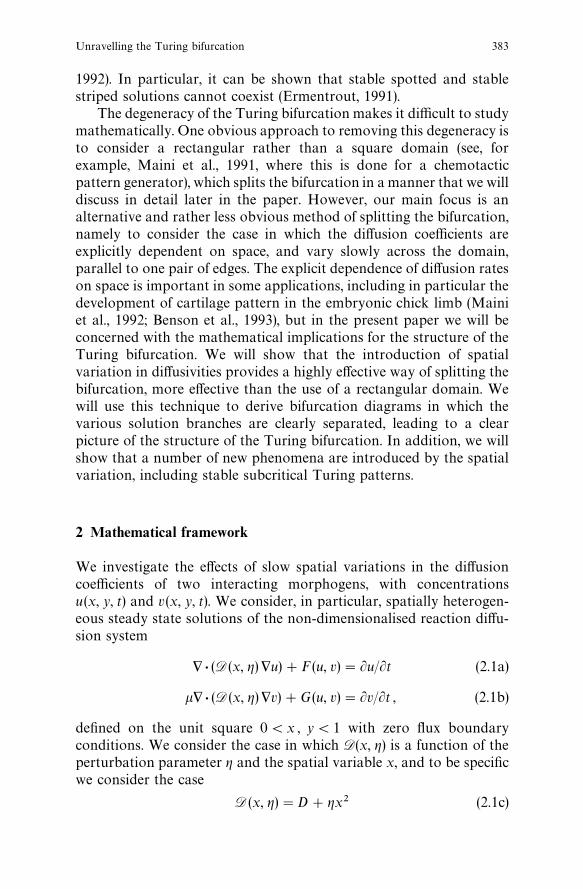
1992). In particular, it can be shown that stable spotted and stablestriped solutions cannot coexist (Ermentrout, 1991).

The degeneracy of the Turing bifurcation makes it difficult to studymathematically. One obvious approach to removing this degeneracy isto consider a rectangular rather than a square domain (see, forexample, Maini et al., 1991, where this is done for a chemotacticpattern generator), which splits the bifurcation in a manner that we willdiscuss in detail later in the paper. However, our main focus is analternative and rather less obvious method of splitting the bifurcation,namely to consider the case in which the diffusion coefficients areexplicitly dependent on space, and vary slowly across the domain,parallel to one pair of edges. The explicit dependence of diffusion rateson space is important in some applications, including in particular thedevelopment of cartilage pattern in the embryonic chick limb (Mainiet al., 1992; Benson et al., 1993), but in the present paper we will beconcerned with the mathematical implications for the structure of theTuring bifurcation. We will show that the introduction of spatialvariation in diffusivities provides a highly effective way of splitting thebifurcation, more effective than the use of a rectangular domain. Wewill use this technique to derive bifurcation diagrams in which thevarious solution branches are clearly separated, leading to a clearpicture of the structure of the Turing bifurcation. In addition, we willshow that a number of new phenomena are introduced by the spatialvariation, including stable subcritical Turing patterns.

2 Mathematical framework

We investigate the effects of slow spatial variations in the diffusioncoefficients of two interacting morphogens, with concentrationsu(x, y, t) and v(x, y, t). We consider, in particular, spatially heterogen-eous steady state solutions of the non-dimensionalised reaction diffu-sion system

+ · (D(x, g) +u)#F(u, v)"Lu/Lt (2.1a)

k+ · (D(x, g)+v)#G (u, v)"Lv/Lt , (2.1b)

defined on the unit square 0(x , y(1 with zero flux boundaryconditions. We consider the case in which D(x, g) is a function of theperturbation parameter g and the spatial variable x, and to be specificwe consider the case

D (x, g)"D#gx2 (2.1c)

Unravelling the Turing bifurcation 383

where D is a positive constant. Crucially, LD/LxP0 as gP0; other-wise there is no special significance in the form (2.1c), and we focus ona particular spatial dependence to enable explicit calculation of thevarious terms in the expansions near bifurcation points. In (2.1),+"(L/Lx

L/Ly ). We take k, the ratio of diffusion coefficients, to be thebifurcation parameter. Standard linear analysis shows that, for par-ticular kinetics F and G and with g"0, there is a critical value k

cof

k at which the uniform steady state loses linear stability. When theuniform steady state is linearly unstable to a single mode, with uniquewavenumber, standard bifurcation theory (Sattinger, 1972) shows thatclose to the bifurcation point there exists a family of analytic solutionsof the form

Au (x)v (x)B"A

u0

v0B#eA

u1(x)

v1(x)B#e2A

u2(x)

v2(x)B#O(e3) (2.2a)

k"kc#eq

1#e2q

2#O(e3) , (2.2b)

where x"(x, y) , (u0, v

0) is the uniform steady state, and DeD@1. Substi-

tuting (2.2) into the full nonlinear system (2.1) and equating powers ofe determines the functions u

i, v

iand the values of q

i. This leads to an

approximate solution of the weakly nonlinear problem (Iooss andJoseph, 1980).

Our work in this paper deals entirely with the particular spatialdependence (2.1c) for the diffusion coefficients. An important relatedproblem is to consider the effects of small, irregular variations indiffusivity or domain geometry, such as would occur in any realbiological system to which one might apply the Turing theory. Al-though the results we will describe have no formal implications for thiscase, they do suggest the intuitive possibility that such variations mighthave a significant effect on the bifurcation structure.

For small non-zero g, we will show that the bifurcation structure ofthe non-linear system may be found using a two parameter perturba-tion technique (Bauer et al., 1975), wherein primary (and certainsecondary) solution branches are expressed as asymptotic expansionsin the two small parameters, g and e.

In this case,

Au(x)v(x)B"A

u0

v0B#e A

u1(x, g)

v1(x, g)B#e2A

u2(x, g)

v2(x, g)B#O(e3) (2.3a)

k"kB(g)#eq

1(g)#e2q

2(g)#O(e3) (2.3b)


where for each i"1, 2, 2

Aui(x, g)

vi(x, g)B"A

u0i(x)

v0i(x)B#gA

u1i(x)

v1i(x)B#g2A

u2i(x)

v2i(x)B#O (g3)

qi(g)"q0

i#gq1

i#g2q2

i#O (g3)

and kB(g) is the primary bifurcation point. For small non-zero g, we

assume that kB(g) lies close to k

cand may be expressed as a power

series in g,

kB(g)"k

c#gw

1#g2w

2#O (g3) . (2.4)

Following standard techniques (Iooss and Joseph, 1980) we scalee such that

DD (u1, v

1) DD"1, S(u

1, v

1), (u

2, v

2)T"0 , (2.5a)

DD (u11, v1

1) DD"1, S(u0

1, v0

1), (u1

1, v1

1)T"0 , (2.5b)

to obtain a unique expression for each solution branch; here the innerproduct is taken as the integral over the unit square domain of thescalar product of the two vectors.

We will show that substituting these expansions into (2.1) andsolving the resulting equations to leading order indicates a splitting ofthe degenerate bifurcation point k

cwhen g90, giving two simple

primary bifurcation points and a secondary bifurcation point, whichlies on one of the primary solution branches. When g is small thesecondary bifurcation point, k

S(g), lies close to the primary bifurcation

point and steady state solutions of the model equations (2.1) may bewritten in terms of their displacement from the primary solutionbranch. In particular, following Mahar and Matkowsky (1977), wewrite the solutions on the secondary branch (denoted uN , vN ) as

AuN (x, d, g)vN (x, d, g)B"AuP(x, g)

vP(x, g)B#d AuN 1(x, g)

vN1(x, g)B#d2AuN 2 (x, g)

vN2(x, g)B#O(d3) (2.6a)

k"kS(g)#dl

1(g)#d2l

2(g)#O(d3) (2.6b)

where for each i"1, 2, 2

AuN i(x, g)vNi(x, g)B"g1@2AuN 1i (x)

vN 1i(x)B#gAuN 2i (x)

vN 2i(x)B#O(g3@2) ,

li(g)"l0

i#g1@2l1

i#gl2

i#O(g3@2) .

Here uP(x, g) denotes the solution vector on the primary bifurcation

branch at the point k"kS(g) at which the secondary bifurcation


occurs. We assume that this secondary bifurcation point correspondsto a value e

B(g) of the parameter e, which depends on g according to the

relationeB"g1@2e

1#g1e

2#O(g3@2) , (2.7)

Fig. 1. A schematic representation of the bifurcation diagram for pattern formation inthe system (2.1) when there is a small spatial variation in the diffusion coefficient,parameterised by g;1. The form of this bifurcation diagram is derived in Sects. 3 and4; stability, which is not shown in this figure, is discussed in Sect. 5. In the spatiallyhomogeneous case (g"0) the Turing bifurcation is highly degenerate; this figureillustrates how the various solution branches separate when spatial inhomogeneity isintroduced. The bifurcation point splits into two separate primary bifurcation points,k"kx

Band k"ky

B, and a secondary bifurcation point k

S. Moreover, the pairs of

solution branches, which are coincident when g"0, separate for non-zero g. Asillustrated schematically, the primary solution branches correspond to striped pat-terns, and the secondary solution branches correspond to spotted patterns. In theseschematic illustrations of pattern type, the x-axis of the square domain runs across thepage, and the y-axis runs up the page. On the figure, the dependence of the variousbranch separations on g are indicated. These are all calculated in the text, although itshould be noted that the separation of the two primary solution branches emergingfrom ky

Bhas not be determined beyond showing that there is no term that is <g2 . All

the other separations have been determined so that the indicated separations are strictorder of magnitude dependencies on g


where e1, e

2, 2 are real and e

190. Here, without loss of generality,

g is assumed positive. In this case, the solutions (2.6) become powerseries expansions in the perturbation parameter g and the small para-meter d, which is a measure of the distance from the secondarybifurcation point. The unknowns, uN j

i, l j

iand e

imay therefore be

determined by substituting the power series expansions into the modelequations and collecting terms of equal power in g and d. The methodof analysis is completely analogous to the determination of the primarysolution branches.

Figure 1 shows a schematic representation of the bifurcation struc-ture when g90. The stability of the various solutions in this structurecan be determined in a standard way, and we will discuss the results ofthis study in Sect. 5.

To be specific, in the numerical simulations illustrated in this paperwe will use the standard non-dimensionalised Schnakenberg kinetics(Schnakenberg, 1979)

F(u, v)"! (A!u#vu2) and G (u, v)"!(B!vu2) , (2.8)

where !, A and B are positive parameters. However, the analyticalresults are quite general.

3 Primary solution branches

Substituting the power series expansions (2.3) into the model equations(2.1) we first collect terms of O(e) and equate them to zero. For g"0,this leads to the linearised system for spatially homogeneous diffusioncoefficients. We assume that this system admits a single unstablewavenumber, denoted by k

c. The general solution for (u1

1, v1

1) (recalling

the zero flux boundary conditions) may therefore be written in the form+

iÈ`jÈ/k#È(Cu

i, j, Cv

i, j) cos(inx) cos ( jny) for some suitably defined con-

stants Cui, j

and Cvi, j

. However, since the domain may be rescaled suchthat k2

c"1 (Ermentrout, 1991) we assume that the first unstable

wavenumbers are (i"1, j"0) and (i"0, j"1). Together with thenormalisation condition, D (u0

1, v0

1) D2"1, this implies that

Au01

v01B"A1mBC

xcos(nx)#C

ycos(ny) , (3.1)

where

m"

Dn2!Fu

Fv

, (3.2)

and

C2x#C2

y"C2,

21#m2

. (3.3)


Here Fudenotes LF/LuD

(uÒ,vÒ)and we extend this notation in the obvious

way, so that for example Guv

denotes L2G/LuLvD(uÒ,vÒ)

.Equating terms to O(g) and using the Fredholm Alternative yields

the solvability conditions

w1Dmpn2

2C

x#(1#k

cmp)A

n2

6!

14BC

x"0 ,

andw1Dmpn2

2C

y#(1#k

cmp)

n2

6C

y"0 ,

where p"(Dn2!Fu)/G

u. Recall that the constant w

1appears in the

expansion of kB(g), defined in equation (2.4). Thus, for a solution to

exist, the unknowns Cx, C

yand w

1must satisfy either

C2x"C2, C

y"0, w

1"wx

1,!

2(1#kcmp)

Dmpn2 An2

6!

14B (3.4a)

or

Cx"0, C2

y"C2, w

1"wy

1,!

2(1#kcmp)

Dmpn2 An2

6 B . (3.4b)

This implies that the degenerate bifurcation point for g"0, at k"kc,

has split into two simple primary bifurcation points given by

kxB"k

c#gwx

1#O (g2) (3.5a)

kyB"k

c#gwy

1#O (g2) . (3.5b)

Note that the splitting of multiple primary bifurcation points in thepresence of small non-zero parameters has been observed for a numberof other systems (see, for example, Bauer et al. (1975) and Reiss (1983)).Hunding and Br+ns (1990) also reported this phenomenon in theirstudy of the effects of spatial variation in a three-dimensional reactiondiffusion model of cell division during early embryonic development.

3.1 The branch bifurcating at kxB

We now proceed to determine leading order power series approxima-tions to the primary solution branches bifurcating from each of kx

Band ky

B. First we consider the family of solutions M(u(x, e, g), v (x, e, g)),

k(e, g)N bifurcating from the primary bifurcation point kxB, defined in

(3.5a). From equations (3.1) and (3.4a) it follows that

Au01(x)

v01(x)B"A

1mBC cos(nx)


where m and C are defined by equations (3.2) and (3.3) respectively. Wecan then determine (u1

1, v1

1) (see Appendix 1) and hence approximate the

primary solution branch by

AuvB"A

u0

v0B#eCAA

1mBcos(nx)#g+

iAaui

aviB cos(inx)D#

higherorderterms

(3.6a)

k"kxB(g)#egq1

1#e2q0

2#higher order terms , (3.6b)

where aui

and avi

(i"1, 2, 2) are constants. Here our notation is asdescribed in Sect. 2, with qj

idenoting the coefficient of eigj in the

expansion of k. In fact the parameter q02

plays a key role in thebifurcation structure, and we will denote it henceforth as qx

2, to

distinguish it from the coefficient of e2 in another expansion, to beintroduced later.

To leading order, the above approximation depends only on thespatial variable x. It may be shown by induction that the whole powerseries expansion is independent of the spatial variable y, and thus thatthe primary solution branch is quasi-one-dimensional. In particular,this implies that (3.6) are power series expansions for steady statesolutions of the one-dimensional reaction diffusion system

LLxD (x, g)

LuLx

#f (u, v)"LuLt

(3.7a)

kLLxD(x, g)

LvLx

#g(u, v)"LvLt

. (3.7b)

The solutions of (3.7) have spatially varying wavelengths of oscillation,and the asymmetry in wavelength increases with the spatial variationinD (Benson et al., 1993). Figure 2 compares the analytical approxima-tions (3.6) for u with numerical solutions of (3.7) for Schnakenbergkinetics (2.8).

There is good qualitative agreement between the solutions for allD g D, D e D(1, but good quantitative agreement holds only when thesystem is close to the bifurcation point and D g D;1. As expected, forvalues of D g D;1, the variations in pattern wavelength and amplitudeare small and are thus hard to detect in numerical simulation, but thespatial asymmetry becomes clearly visible as g is increased.

Figure 2c compares the approximation for u in two spatial dimen-sions. Since the primary solutions depend only on the spatial variablex, they predict spatial patterns which represent stripes perpendicular to


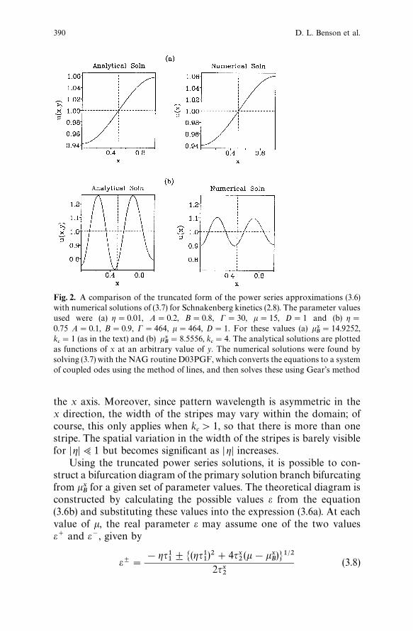
Fig. 2. A comparison of the truncated form of the power series approximations (3.6)with numerical solutions of (3.7) for Schnakenberg kinetics (2.8). The parameter valuesused were (a) g"0.01, A"0.2, B"0.8, C"30, k"15, D"1 and (b) g"0.75 A"0.1, B"0.9, C"464, k"464, D"1. For these values (a) kx

B"14.9252,

kc"1 (as in the text) and (b) kx

B"8.5556, k

c"4. The analytical solutions are plotted

as functions of x at an arbitrary value of y. The numerical solutions were found bysolving (3.7) with the NAG routine D03PGF, which converts the equations to a systemof coupled odes using the method of lines, and then solves these using Gear’s method

the x axis. Moreover, since pattern wavelength is asymmetric in thex direction, the width of the stripes may vary within the domain; ofcourse, this only applies when k

c'1, so that there is more than one

stripe. The spatial variation in the width of the stripes is barely visiblefor D gD;1 but becomes significant as D gD increases.

Using the truncated power series solutions, it is possible to con-struct a bifurcation diagram of the primary solution branch bifurcatingfrom kx

Bfor a given set of parameter values. The theoretical diagram is

constructed by calculating the possible values e from the equation(3.6b) and substituting these values into the expression (3.6a). At eachvalue of k, the real parameter e may assume one of the two valuese` and e~, given by

eB"

!gq11$M(gq1

1)2#4qx

2(k!kx

B)N1@2

2qx2

(3.8)


Fig. 3. A comparison of bifurcation diagrams constructed from the truncated powerseries approximations (left) from (3.6) with those produced by AUTO (right). Theparameter values used are as in Fig. 2(a) with the exception that in (a) g"0.05 and(b) g"0.5. In this case, our analysis predicts that (a) k

B+k

Lwith value 15.0028, and

in (b) kB"15.878, k

L"15.875. In turn AUTO predicts that in (a) k

B+k

Lwith value

15.006 and in (b) kB"16.194, k

L"16.1649

Thus the power series expansion (3.6) represents two solutionsu(x, e`, g) and u (x, e~, g) of different magnitude, and on the bifurcationdiagram (Fig. 3), where we plot k against the maximum value ofDDu(x, e, g) DD, there will appear two distinct arms of the primary solutionbranch. This separation of the branches when g90 represents anadditional splitting of the Turing bifurcation in comparison to the caseg"0, when the two branches are coincident, representing identicalpatterns but with opposite polarity. In practice, the difference betweenDDu(x, e~, g) DD and DDu(x, e`, g) DD is barely visible at very small values of g,but as the magnitude of g increases, the two arms of the primarysolution branch may be distinguished in numerical simulations.


When qx2'0, one arm is supercritical but the other has a small

subcritical region. On this second arm, the point k"kL, e"e

L, where

kL"k

B!(gq1

1)2/(4qx

2) and e

L"!gq1

1/(2qx

2), represents a simple limit

point at which the branch changes direction. This implies that for eachk 3 [k

L, kx

B] there exist two subcritical solutions lying on the same arm

of the primary solution branch, whilst for each k'kxB

there exist twosupercritical solutions lying on different arms. A similar result holdswhen qx

2(0. Thus, for g90, the uniform steady state undergoes

a transcritical bifurcation at the point kxB. This contrasts to the case

g"0, where the uniform steady state undergoes a pitchfork bifurca-tion, and primary solution branches represent stripes perpendicular tothe x axis which are supercritical when qx

2'0 and subcritical when

qx2(0 (see later).Since the primary solution branch bifurcating from kx

Bis quasi-one-

dimensional we may compare our theoretical bifurcation diagram withone produced by the numerical package AUTO (Doedel, 1986), whichlocates the bifurcation and limit points of a partial differential equationsystem defined in one spatial dimension and constructs the associatedsolution branches by a pseudo arc length continuation method. A com-parison of the bifurcation diagrams is illustrated in Fig. 3, where thebifurcation parameter k is plotted against the maximum amplitude ofDDu(x, y) DD. Again, there is good qualitative agreement for all 0(DgD(1and 06DeD(1, but only good quantitative agreement when the systemis close to the bifurcation point (i.e. e;1 and DgD;1). In particular,these numerical results confirm that in contrast to the case g"0, thereare stable subcritical striped solutions (Fig. 4). This is discussed inmore detail in Sect. 5, when we consider the stability of the solutionbranches.

3.2 The branch bifurcating at kyB

Similar analysis can to used to calculate the power series expansionsfor the primary solution branch bifurcating from ky

B(see Appendix 1 for

details) and we find that

AuvB"A

u0

v0B#eCAA

1mBcos(ny)

#g +iAbu

ibviB cos (inx)cos(ny)D#

higherorderterms

(3.9a)

k"kyB(g)#e2qx

2#higher order terms , (3.9b)


Fig. 4. An example of a subcritical stable steady solution of (2.1) represented in oneand two spatial dimensions. The solution on the right was obtained by numericalsolution of (3.7), on the interval [0, 1], with the NAG routine D03PGF. The solutionon the left was found by solving the full non-linear reaction diffusion system (2.1) on theunit square using a finite difference scheme to obtain a system of algebraic equationswhich were solved by an alternating direction implicit (ADI) method. The analysispresented in Appendix 2 predicts that this pattern is stable. In this example,Schnakenberg kinetics were used with parameter values as in Fig. 1(a) except thatg"1.2 and k"19.06. AUTO predicts k

B"19.2443 and k

L"18.9987. Since the

uniform steady state is also stable in this parameter range, initial conditions close tothe theoretically predicted pattern were used to generate the solution

where bui, bv

i(i"1, 2, 2) are constants. Again we replace the coeffic-

ient q02

of e2 by qx2, since detailed calculation (see Appendix 1) shows

that the coefficient of e2 here is the same as that in the expansion (3.6b)at kx

B, namely qx

2, whose value is given in (A.5) in Appendix 1. For g90

it is seen that the power series expansion is dependent on both spatialvariables and, in general, has no planes of symmetry. However, thex-dependence lies in a O(eg) term, that is of a lower order of magnitudethan the x-independent O (e) term as gP0. Therefore, the truncatedform of the power series approximation predicts stripes perpendicularto the y axis whose spatial variation is O(g) as gP0. Typical examplesare illustrated in Fig. 5.

As before, there is good qualitative agreement between the solu-tions for all 0(D g D(1 and 06D e D(1, but the quantitative agree-ment is best close to the bifurcation point (e;1), when D g D;1. In thiscase, the asymmetries introduced into the wavelength and amplitudeare small and barely visible in simulations. As the magnitude ofg increases, however, significant spatial asymmetry may be observed inthe spatial patterns. Again, the pattern variation is captured by thetruncated solutions in this case, since the terms egu1

1and eu0

1are

comparable.Using (3.9), the bifurcation diagram for the primary solution

branch bifurcating from kyB

may also be constructed. For each value of


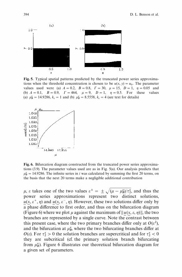
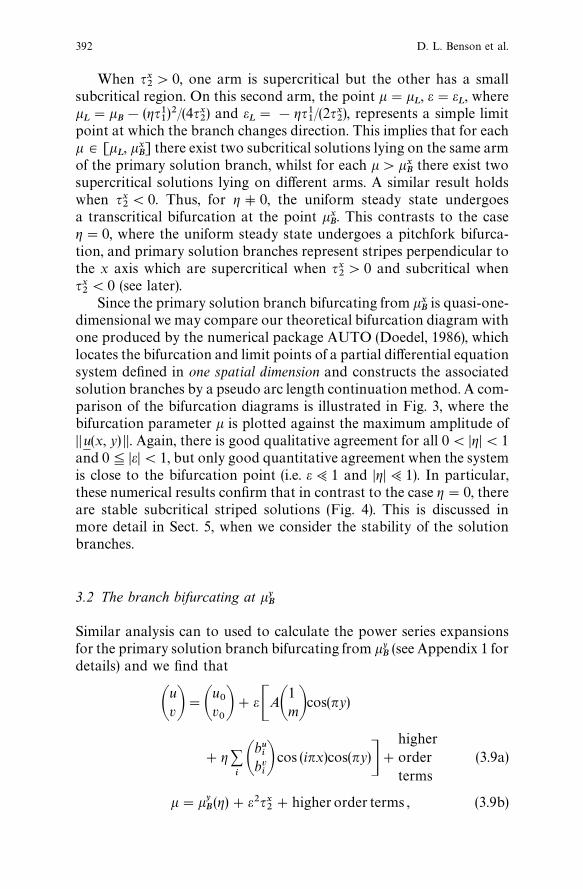
Fig. 5. Typical spatial patterns predicted by the truncated power series approxima-tions when the threshold concentration is chosen to be u(x, y)"u

0. The parameter

values used were (a) A"0.2, B"0.8, C"30, k"15, D"1, g"0.05 and(b) A"0.1, B"0.9, C"464, k"9, D"1, g"0.5. For these values(a) ky

B"14.9286, k

c"1 and (b) ky

B"8.5558, k

c"4 (see text for details)

Fig. 6. Bifurcation diagram constructed from the truncated power series approxima-tions (3.9). The parameter values used are as in Fig. 5(a). Our analysis predicts thatkyB"14.9286. The infinite series in i was calculated by summing the first 20 terms, on

the basis that the next 20 terms make a negligible additional contribution

k, e takes one of the two values eB"$J(k!kyB)/qx

2, and thus the

power series approximations represent two distinct solutions,u(x, e`, g) and u(x, e~, g). However, these two solutions differ only bya phase difference to first order, and thus on the bifurcation diagram(Figure 6) where we plot k against the maximum of DDu (x, e, g) DD, the twobranches are represented by a single curve. Note the contrast betweenthis present case, where the two primary branches differ only at O(e2),and the bifurcation at kx

B, where the two bifurcating branches differ at

O(e). For qx2'0 the solution branches are supercritical and for qx

2(0

they are subcritical (cf. the primary solution branch bifurcatingfrom kx

B). Figure 6 illustrates our theoretical bifurcation diagram for

a given set of parameters.


3.3 Primary bifurcations when g"0

To compare the primary bifurcation structure when g90 withthat when g"0, that is, the case of spatially homogeneous coefficients,we have used the above technique to show that when g"0 there arethree distinct primary solution branches bifurcating from k

cof the

form:

AuvB"A

u0

v0B#eA

1mBC cos(nx)

#e2GAauavB

iC2cos(2nx)2

#AbubvBiC2

2 H#O (e3)

k"kc#e2qx

2#O(e3) , (3.10)

which represents stripes perpendicular to the x axis,

AuvB"Au0v0B#eA1mBC cos(ny)

#e2GAau

avBiC2cos(2ny)

2#A

bu

bvBiC2

2 H#O (e3)

k"kc#e2qx

2#O(e3) , (3.10b)

which represents stripes perpendicular to the y axis, and

AuvB"A

u0

v0B#eA

1mBCx

cos(nx)#Cycos(ny))

#e2GAauavBi(C2

xcos(2nx)#C2

ycos(2ny))

2

#Abu

bvBi (C2

x#C2

y)

2#A

cu

cvBCx

Cycos(nx)cos(ny)H#O(e3)

k"kc#e2qxy

2#O(e3) (3.10c)

(C2y#C2

x"C2) which represents spotted solutions. Here i"

12Fuu#F

uv, and the constants a

u, a

v, b

u, b

v, c

uand c

vare defined in

Appendix 1. Recall that, without loss of generality, we assume thatkc"1. Strictly speaking the last power series expansion represents two


distinct solution branches, one for which Cx"C

yand the other for

which Cx"!C

y. The parameter qxy

2, which is in general non-zero, is

defined by the equation

Dmpn2qxy2

2#(!1#p) i

C2

2(F

uu#mF

uv)A

au8#

bu

2#

cu2B

#(!1#p)iC2

2Fuv A

av

8#

bv

2#

cv2B#(!1#p)F

uuv

9C2

16"0 (3.11)

The power series expansions above are in agreement with the wellknown fact that, in the case of constant diffusion coefficients andzero flux boundary conditions, the uniform steady state undergoesa pitchfork bifurcation. In particular, striped solution branches aresupercritical when qx

2'0 and subcritical when qx

2(0, whilst the spot-

ted solution branches are supercritical when qxy2'0 and subcritical

when qxy2(0. Thus, in contrast to the case g90, there are no tran-

scritical bifurcations.Comparing equations (3.6) and (3.10a), it is clear that the solution

branch bifurcating from kxB

when g90 represents a perturbation fromthe striped solution branch perpendicular to the x axis when g"0.Similarly, the solution branch (3.9) bifurcating from ky

Bwhen g90

represents a perturbation from the striped solution branch (3.10b)perpendicular to the y axis when g"0. Moreover, our analysis showsin detail how the different bifurcation points and branches collapse asgP0 to give the degenerate structure described above (see Fig. 1).However, when g90, there is no primary solution branch analogousto the spotted solution branch (3.10c) when g"0. In the followingsection we show that this is due to a further splitting of the primarybifurcation point so that spots arise as secondary bifurcations fromprimary striped solution branches.

4 Secondary bifurcations

In this section we determine secondary bifurcations of the modelsystem (2.1) which occur close to the primary bifurcation points kx

Band

kyB

using the method outlined in Sect. 2. We recall from (2.6) ournotation that u

P(x, g) represents the solution on the primary solution

branch at the point at which a secondary bifurcation occurs, namelyk"k

S(g) or equivalently e"e

B(g). When the secondary bifurcation

point lies on the primary solution branch bifurcating from kxB, the


solution is

AuxP(g)

vxP(g)B"A

u0

v0B#g1@2A

1mBC e

1cos(nx)

#gAauavB

iC2e21cos(2nx)2

#gAcucvB

iC2e21

2

#g A1mBCe2cos(nx)#O (g3@2) (4.1a)

withkxS(g)"k

c#g (wx

1#qx

2e21)#O(g3@2) , (4.1b)

and when it lies on the solution branch bifurcating from kyB, it is

AuyP(g)

vyP(g)B"Au0v

0B#g1@2A1mBCe

1cos(ny)#gAaua

vBiC2e2

1cos(2ny)2

#gAcucvB

iC2e21

2#g A1mBCe

2cos(ny)#O (g3@2) (4.2a)

withkS(g)"k

c#g (wy

1#qx

2e21)#O (g3@2) . (4.2b)

Here the constants e1

and e2

are coefficients of powers of g1@2 in theexpansion (2.7) of e

B(g); these constants remain to be determined. The

various other constants were defined during the determination of theprimary solution branch (Sect. 3 and Appendix 1).

In the power series expansion (2.6) of the secondary solutionbranch, the variable d is analogous to the parameter e along theprimary solution branches. In particular, d provides a measure of thedistance from k

Sand is scaled such that

DD (uN 11, vN 1

1) DD"1, S(uN 1

1, vN 1

1), (uN 1

2, vN 1

1)T"0 . (4.3)

With this choice of scaling, however, d is singular at g"0. Thus, incontrast to the power series expansions for the primary solutionbranches, analytical approximations of the form (2.6) only exist fornon-zero g. This reflects the fact that for g"0, secondary bifurcationsdo not generally occur close to the primary bifurcation point, so thatsecondary solution branches may not be written in terms of theirdisplacement from a small amplitude primary solution, as in the powerseries expansions (2.6). There may be other choices for the para-meterisation of the secondary solution branches which are non-singu-lar as gP0, but for g90, the d and g expansion (2.6) is the mostnatural parameterisation of the secondary solution branch, and is thusthe one we use.


First we consider the secondary bifurcation points which lie alongone of the primary solution branches bifurcating from kx

B. At O(dg1@2),

we have

AuN 11vN 11B"A1mB (C

xcos(nx)#C

ycos(ny)) ,

where (C2x#C2

y)"C2"2/(1#m2).

To O (g), the Fredholm Alternative forces l11"0. In this case

AuN 21

vN 21B"A

au

avB2iCe

1C

xcos(2nx)

2#A

bu

bvB2iCe

1C

x2

#Acu

cvB2iCe

1C

ycos(nx)cos(ny) . (34)

The value of e1

may now be determined by collecting the terms atO(g3@2). The solvability conditions become (after much tedious algebra)

Cx

Dmpn2(wx1#qx

2e21)

2#C

x(1#k

cmp)A

n2

6!

14B

#Cx(!1#p)iC2e2

1FuvA

3av

8#

3bv

4 B#C

x(!1#p)iAC2e2

1(F

uu#F

uvm)A

3au

8#

3bu

4 BB#C

x(!1#p)

9Fuuv

mC2e21

16#C

xDmpn2l2

1Ce

1"0 ,

and

Cy

Dmpn2(wx1#qx

2e21)

2#C

y

(1#kcmp)n2

6

#Cy(!1#p) iC2e2

1F

uvAbv

4#

cv2B

#Cy(!1#p)iC2e2

1(F

uu#F

uvm)A

bu

4#

cu2B

#Cy(!1#p)

3Fuuv

mC2e21

8"0 .

From these equations we deduce that either

C2x"C2, C

y"0, l2

1"2e

1qx2, (4.5)


or

Cx"0, C2

y"C2, l2

1"0 (4.6a)

and

e21G(!1#p) [C2(F

uu#F

uvm) A

bu

4#

cu2B#C2F

uvAbv

4#

cv2BD

#

3C2Fuuv

8#

Dmpn2 qx2

2 H#Dmpn2wx

12

#

(1#kcmp)n2

6"0 . (4.6b)

In the former case (4.5), the value of e1

is undetermined. This is a trivialcase, in which the corresponding power series expansion (2.6) repres-ents the continuation of the primary solution branch beyond thesecondary bifurcation point, and may be obtained by replacing e bye1#dg1@2 in our original analytical approximation of the primary

solution branch.To determine the secondary bifurcations, we must therefore consider

(4.6). In this case there exists a secondary bifurcation point of the form(2.7) whenever equation (4.6) admits a real, non-zero solution for e

1.

This requires (wxÇ~wyÇ)2(qxyÈ ~qxÈ)

'0, where qxy2

is defined by the equation (3.11).When this condition is satisfied

e1"e

x"$S

(wx1!wy

1)

2(qxy2!qx

2), (4.7)

and equation (2.7) defines two distinct secondary bifurcation points.Moreover, since the corresponding values of e have opposite signs,these points lie on separate arms of the primary solution branch, but atthe same value of k (at least to this order), namely

k"kxS(g),k

c#gAwx

1#

qx2(wx

1!wy

1)

2(qxy2!qx

2) B (4.8)

By a similar analysis, we find that two secondary bifurcation points ofthe form (2.7) can occur on the primary solution branch bifurcatingfrom ky

B. In this case, however, we require (wxÇ~wyÇ)2(qxyÈ ~qxÈ)

(0. Again bothsecondary bifurcations occur on separate primary solution branches atthe same value of k to leading order, which is

kyS(g)"k

c#gAwy

1#

qx2(wy

1!wx

1)

2(qxy2!qx

2) B . (4.9)

Thus a secondary bifurcation of the form (2.7) occurs on exactly one ofthe primary solution branches. Specifically, the secondary bifurcationpoints lie on the primary solution branch bifurcating from kx

Bwhen


(wxÇ~wyÇ)

2(qxyÈ ~qxÈ)'0 and on the primary solution branch bifurcating from

kyB

when (wxÇ~wyÇ)2(qxyÈ ~qxÈ)(0. Each of these cases are therefore considered

separately.

4.1 Solutions on the secondary branches

We can determine the leading order approximations to the secondarysolution branches bifurcating from kx

Sand ky

S. We find, after a great

deal of tedious algebra, that the power series expansion for the second-ary solution branch bifurcating from kx

Sis given by

AuvB"Au0v0B#g1@2A1mBCe

xcos(nx)

#gAauavBiC2e2

xcos(2nx)2

#gAbubvBiC2e2

x2

#O (g3@2)

#dGg1@2A1mBCcos(ny)#gA

cu

cvBi2C2e

xcos(nx)cos(ny)#O(g3@2)H

#d2Gg1@2A1mBCcos(nx)

2ex

#gAauavBiC2

cos(2nx)#cos(2ny)2

.

#gAbu

bvBiC2e2

x#O(g3@2) H#O (d3) (4.10a)

k"kc#(wx

1#qx

2e2x)g#d2g2qxy

2#O(d3) . (4.10b)

By a similar analysis we may determine the secondary solutionbranches bifurcating from ky

S. In this case the power series expansions

have the form

AuvB"A

u0

v0B#g1@2A

1mBCe

ycos(ny)

#gGAauavBi

C2e2ycos(2ny)2

#AbubvBi

C2e2y

2 H#O(g3@2)

#dGg1@2A1mBCcos(nx)#gA

cu

cvB2iC2e

ycos(nx)cos(ny)#O(g3@2)H

#d2Gg1@2A1mBCcos(ny)

2ey

#gAauavBiC2

cos(2nx)#cos(2ny)2

#gAbu

bvBiC2#O (g3@2)H#O (d3)


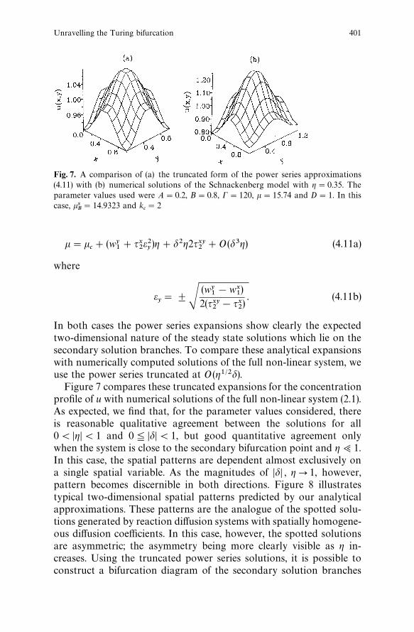
Fig. 7. A comparison of (a) the truncated form of the power series approximations(4.11) with (b) numerical solutions of the Schnackenberg model with g"0.35. Theparameter values used were A"0.2, B"0.8, C"120, k"15.74 and D"1. In thiscase, ks

B"14.9323 and k

c"2

k"kc#(wy

1#qx

2e2y)g#d2g2qxy

2#O(d3g) (4.11a)

where

ey"$S

(wy1!wx

1)

2(qxy2!qx

2). (4.11b)

In both cases the power series expansions show clearly the expectedtwo-dimensional nature of the steady state solutions which lie on thesecondary solution branches. To compare these analytical expansionswith numerically computed solutions of the full non-linear system, weuse the power series truncated at O (g1@2d).

Figure 7 compares these truncated expansions for the concentrationprofile of u with numerical solutions of the full non-linear system (2.1).As expected, we find that, for the parameter values considered, thereis reasonable qualitative agreement between the solutions for all0(DgD(1 and 06DdD(1, but good quantitative agreement onlywhen the system is close to the secondary bifurcation point and g;1.In this case, the spatial patterns are dependent almost exclusively ona single spatial variable. As the magnitudes of DdD , gP1, however,pattern becomes discernible in both directions. Figure 8 illustratestypical two-dimensional spatial patterns predicted by our analyticalapproximations. These patterns are the analogue of the spotted solu-tions generated by reaction diffusion systems with spatially homogene-ous diffusion coefficients. In this case, however, the spotted solutionsare asymmetric; the asymmetry being more clearly visible as g in-creases. Using the truncated power series solutions, it is possible toconstruct a bifurcation diagram of the secondary solution branches


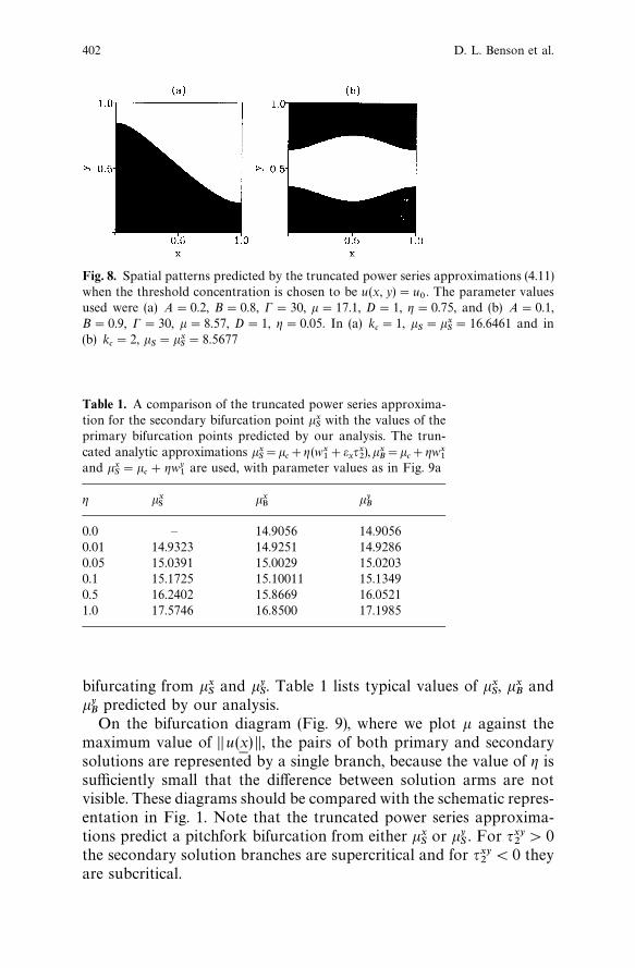
Fig. 8. Spatial patterns predicted by the truncated power series approximations (4.11)when the threshold concentration is chosen to be u(x, y)"u

0. The parameter values

used were (a) A"0.2, B"0.8, C"30, k"17.1, D"1, g"0.75, and (b) A"0.1,B"0.9, C"30, k"8.57, D"1, g"0.05. In (a) k

c"1, k

S"kx

S"16.6461 and in

(b) kc"2, k

S"kx

S"8.5677

Table 1. A comparison of the truncated power series approxima-tion for the secondary bifurcation point kx

Swith the values of the

primary bifurcation points predicted by our analysis. The trun-cated analytic approximations kx

S"k

c#g(wx

1#e

xqx2),kx

B"k

c#gwx

1and kx

S"k

c#gwy

1are used, with parameter values as in Fig. 9a

g kxS

kxB

kyB

0.0 — 14.9056 14.90560.01 14.9323 14.9251 14.92860.05 15.0391 15.0029 15.02030.1 15.1725 15.10011 15.13490.5 16.2402 15.8669 16.05211.0 17.5746 16.8500 17.1985

bifurcating from kxS

and kyS. Table 1 lists typical values of kx

S, kx

Band

kyB

predicted by our analysis.On the bifurcation diagram (Fig. 9), where we plot k against the

maximum value of DDu(x) DD, the pairs of both primary and secondarysolutions are represented by a single branch, because the value of g issufficiently small that the difference between solution arms are notvisible. These diagrams should be compared with the schematic repres-entation in Fig. 1. Note that the truncated power series approxima-tions predict a pitchfork bifurcation from either kx

Sor ky

S. For qxy

2'0

the secondary solution branches are supercritical and for qxy2(0 they

are subcritical.


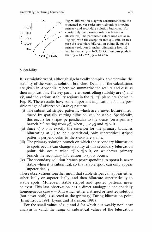
Fig. 9. Bifurcation diagram constructed from thetruncated power series approximations showingprimary and secondary solution branches. (Forclarity only one primary solution branch isillustrated.) The parameter values used are as inFig. 9(a) with the exception that g"0.01. In thiscase the secondary bifurcation points lie on theprimary solution branches bifurcating from kx

B,

and has value kxS"14.9323. Our analysis predicts

that kxB"14.9252, ky

B"14.9286

5 Stability

It is straightforward, although algebraically complex, to determine thestability of the various solution branches. Details of the calculationsare given in Appendix 2; here we summarise the results and discusstheir implications. The key parameters controlling stability are qx

2and

qxy2

, and the various stability regions in the qx2— qxy

2plane are shown in

Fig. 10. These results have some important implications for the pos-sible range of observable (stable) patterns:(i) The subcritical striped patterns, which are a novel feature intro-

duced by spatially varying diffusion, can be stable. Specifically,this occurs for stripes perpendicular to the x-axis (on a primarybranch bifurcating from kB

x) when k

L(kx

Band qx

2'0.

(ii) Since qx2'0 is exactly the criterion for the primary branches

bifurcating at kyB

to be supercritical, only supercritical stripedpatterns perpendicular to the y-axis are stable.

(iii) The primary solution branch on which the secondary bifurcationto spots occurs can change stability at this secondary bifurcationpoint; this occurs when qxy

2'qx

2'0, on whichever primary

branch the secondary bifurcation to spots occurs.(iv) The secondary solution branch (corresponding to spots) is never

stable when it is subcritical, so that stable spots can only appearsupercritically.

These observations together mean that stable stripes can appear eithersubcritically or supercritically, and then bifurcate supercritically tostable spots. Moreover, stable striped and spotted patterns neverco-exist. This last observation has a direct analogy in the spatiallyhomogeneous case g"0, in which either a striped or spotted solution(but never both) is selected at the (primary) Turing bifurcation point(Ermentrout, 1991; Lyons and Harrison, 1991).

For the small values of e, g and d for which our weakly nonlinearanalysis is valid, the range of subcritical values of the bifurcation


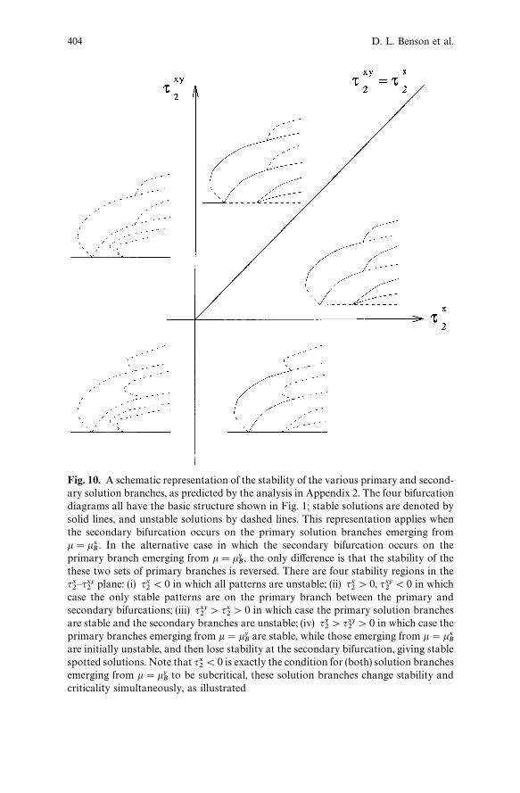
Fig. 10. A schematic representation of the stability of the various primary and second-ary solution branches, as predicted by the analysis in Appendix 2. The four bifurcationdiagrams all have the basic structure shown in Fig. 1; stable solutions are denoted bysolid lines, and unstable solutions by dashed lines. This representation applies whenthe secondary bifurcation occurs on the primary solution branches emerging fromk"kx

B. In the alternative case in which the secondary bifurcation occurs on the

primary branch emerging from k"kyB, the only difference is that the stability of the

these two sets of primary branches is reversed. There are four stability regions in theqx2—qxy

2plane: (i) qx

2(0 in which all patterns are unstable; (ii) qx

2'0, qxy

2(0 in which

case the only stable patterns are on the primary branch between the primary andsecondary bifurcations; (iii) qxy

2'qx

2'0 in which case the primary solution branches

are stable and the secondary branches are unstable; (iv) qx2'qxy

2'0 in which case the

primary branches emerging from k"kyB

are stable, while those emerging from k"kxB

are initially unstable, and then lose stability at the secondary bifurcation, giving stablespotted solutions. Note that qx

2(0 is exactly the condition for (both) solution branches

emerging from k"kyB

to be subcritical, these solution branches change stability andcriticality simultaneously, as illustrated


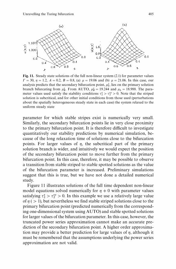
Fig. 11. Steady state solutions of the full non-linear system (2.1) for parameter valuesC"30, g"1.2, A"0.2, B"0.8, (a) k"19.06 and (b) k"21.06. In this case, ouranalysis predicts that the secondary bifurcation point, kx

S, lies on the primary solution

branch bifurcating from kxB. From AUTO, kx

B"19.244 and k

L"18.988. The para-

meter values used satisfy the stability conditions qx2'qxy

2'0. Note that the striped

solution is subcritical, and for other initial conditions from those used (perturbationsabout the spatially heterogeneous steady state in each case) the system relaxed to theuniform steady state

parameter for which stable stripes exist is numerically very small.Similarly, the secondary bifurcation points lie in very close proximityto the primary bifurcation point. It is therefore difficult to investigatequantitatively our stability predictions by numerical simulation, be-cause of the long relaxation time of solutions close to the bifurcationpoints. For larger values of g, the subcritical part of the primarysolution branch is wider, and intuitively we would expect the positionof the secondary bifurcation point to move further from the primarybifurcation point. In this case, therefore, it may be possible to observea transition from stable striped to stable spotted solutions as the valueof the bifurcation parameter is increased. Preliminary simulationssuggest that this is true, but we have not done a detailed numericalstudy.

Figure 11 illustrates solutions of the full time dependent non-linearmodel equations solved numerically for g90 with parameter valuessatisfying qx

2'qxy

2'0. In this example we use a relatively large value

of g ('1), but nevertheless we find stable striped solutions close to theprimary bifurcation point (predicted numerically from the correspond-ing one-dimensional system using AUTO) and stable spotted solutionsfor larger values of the bifurcation parameter. In this case, however, thetruncated power series approximation cannot make an accurate pre-diction of the secondary bifurcation point. A higher order approxima-tion may provide a better prediction for large values of g, although itmust be remembered that the assumptions underlying the power seriesapproximation are not valid.


We complete this section by comparing the stability of striped andspotted solutions of the reaction diffusion system (2.1) for g90 withthe stability of similar solutions in the spatially homogeneous caseg"0. When the diffusion coefficients are constant, a similar analysis tothat in Appendix 2 may be used to determine the stability of theprimary solution branches bifurcating from k

c, via power series expan-

sions (2.2). In this case we find that primary striped solutions are stableif and only if qxy

2'qx

2'0, and that primary spotted solutions are

stable if and only if qx2'qxy

2'0. These conditions are a statement of

the well known fact that for constant diffusion the primary solutionbranches are stable only when the pitchfork bifurcation from theuniform steady is supercritical. Moreover, they agree with recent ana-lyses which show that simultaneously stable striped and spotted solu-tions cannot exist (Ermentrout, 1991; Lyons and Harrison, 1991). Itmay also be shown that, when the model equations are written in termsof displacement from the uniform steady state, the absence of quadraticterms forces (qxy

2!qx

2)(0. Our stability conditions are therefore in

agreement with the fact that certain kinetics exclude stable spottedsolutions.

Moreover, the conditions for stable spotted solutions are the samefor both g"0 and g90. The conditions for the stability of stripedsolutions when g90, however, are the same as for constant diffusiononly beyond the secondary bifurcation point. In this case, the spatialpattern selected for either g"0 or g90 is determined by the competi-tion between cubic and quadratic terms in the kinetics. For values ofthe bifurcation parameter less than the secondary bifurcation value,however, a striped solution is always selected. Thus, a reaction diffu-sion system, which for a given set of parameter values and constantdiffusion coefficients admits only stable spotted solutions, can beforced to generate stable striped solutions by spatially heterogeneousdiffusion coefficients. Numerical simulations demonstrate that thismay also occur when reaction kinetics are spatially heterogeneous orwhen the shape of the domain is rectangular (Lyons and Harrison,1992).

6 Discussion

In this paper we have considered only square shaped domains. Forconstant diffusion coefficients this ensures that no predescribed asym-metry is imposed on the reaction diffusion system which might influ-ence pattern selection. Analytically we have shown, however, thata small spatial asymmetry in diffusion coefficients is sufficient to


exclude the formation of spotted solutions close to a primary bifurca-tion point. This results from the splitting of the primary bifurcationpoint, which for constant diffusion is highly degenerate, into twosimple primary bifurcation points and a secondary bifurcation point.In this respect the bifurcation structure of reaction diffusion systemsdefined on square domains with spatially heterogeneous diffusioncoefficients is similar to that of systems defined on rectangular domainswith constant diffusion coefficients. In the latter case, striped steadystate solutions parallel to the x and y axes generally bifurcate fromdistinct primary bifurcation points. On an almost square domain wehave found that the two primary bifurcation points lie close togetherand spotted solutions appear as secondary bifurcations from one of theprimary solution branches. In contrast to the case of spatially hetero-geneous diffusion coefficients, however, there are no transcritical bifur-cations from the uniform steady state and hence no stable stripedsolutions for subcritical values of the bifurcation parameter. Thisimplies that the two systems are not isomorphic. Moreover, the fourprimary bifurcation branches only separate into two identical pairs onan almost square domain, whereas with spatially varying diffusioncoefficients, all four primary branches become distinct. Thus theintroduction of a small spatial variation in the diffusion co-efficients is a more effective way of splitting the degeneracies in theTuring bifurcation.

Reaction diffusion systems with constant diffusion coefficients de-fined on infinite domains do not in general have stable subcriticalstriped solutions. In this case, there are three basic patterns whichtessellate the plane and appear as steady state solutions of reactiondiffusion systems. These are stripes, rhombs (which correspond to ourspotted solutions) and hexagons (which are not possible on a rectangu-lar or square domain). According to stability analysis (see, for example,Malomed and Tribel’skii, 1987), hexagonal patterns should appear firstvia a subcritical bifurcation. These patterns are stable but becomeunstable at a supercritical value of the bifurcation parameter. From thesame primary bifurcation point, stripes bifurcate supercritically. Theseare unstable close to the bifurcation point, but become stable at largevalues of the bifurcation parameter. There is a region of bistabilitywhere both stripes and hexagons are stable. As on the finite domain,stable spots can form in place of stable stripes.

These theoretical predictions have been confirmed numerically forthe Schnakenberg and Brussellator models (Dufiet and Boissonade,1992a,b; De Wit et al., 1992). Our analysis suggests, however, thatspatially heterogeneous diffusion coefficients could enable striped solu-tions to appear subcritically on an infinite domain. Although both


numerical (Borcksman et al., 1992) and theoretical analyses (Walgraefand Schiller, 1987) have been carried out on systems with spatiallyinhomogeneous model parameters defined on infinite domains, to ourknowledge, subcritical striped solutions have not been reported. Re-cently, however, such solutions were observed (Jensen et al., 1993) innumerical solutions of a reaction diffusion system, defined on a spa-tially homogeneous domain, in which the instability interval of a timeperiodic, spatially oscillating solution overlapped with that of a Turingpattern. The same system also produced spatial patterns which couldbe localised within the domain. In both cases, the spatial patterns wereconstant in time for a wide range of parameter values. In general,however, when a Turing instability and a time oscillatory instabilityoccur simultaneously, the solutions are complex, spatially in-homogeneous, non-stationary structures (Perraud et al., 1993), whichmay be observed experimentally. This has led to the suggestion that bycontinuously varying the value of a single parameter, one might movefrom stationary Turing patterns, through spatio-temporal structures,to travelling excitable waves (Boissonade, 1994). In particular, thishighlights the fact that reaction diffusion mechanisms have a fargreater capacity for pattern formation than is suggested by the linearanalysis of standard Turing systems.

Appendix 1

In this Appendix, we summarise the analytical determination of theprimary solution branches, supplying various details that were omittedin Sect. 3.

A1.1 The branch bifurcating at kxB

Substituting the expansion (2.3b) for k into the governing reactiondiffusion equations (2.1) and equating powers of eg, we find that (u1

1, v1

1)

is a solution of the equation

¸Au11(x1)

v11(x1)B"x2A

1kcmBCn2 cos (nx)#2xA

1kcmBCn sin(nx)

#Dwx1A

0mBCn2 cos(nx), (A.1)

where ¸ is the linearised operator for the nonlinear system (2.1). Recallthat the parameters m, C and wx

1are defined in (3.2), (3.3) and (3.4)


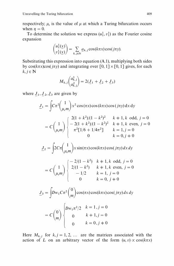
respectively; kcis the value of k at which a Turing bifurcation occurs

when g"0.To determine the solution we express (u1

1, v1

1) as the Fourier cosine

expansion

Au11(x1)

v11(x1)B" +

k, j|Na1 k, j

cos(knx) cos( jny).

Substituting this expression into equation (A.1), multiplying both sidesby cos(knx)cos( jny) and integrating over [0, 1]][0, 1] gives, for eachk, j3N

Mk, j A

a1k, j

a2k, jB"2(J

1 1#J

1 2#J

1 3)

where J1 1

, J1 2

, J1 3

are given by

J1"PCn2A

1kcmBx2 cos (nx) cos (knx) cos ( jny) dx dy

"CA1

kcmB G

2(1#k2)/(1!k2)2!2(1#k2)/(1!k2)2

n2[1/6#1/4n2]0

k91, k odd, j"0k91, k even, j"0k"1, j"0k"0, j90

J2"P2CnA

1kcmBx sin(nx) cos(knx) cos( jny) dx dy

"CA1

kcmB G

!2/(1!k2)2/(1!k2)!1/2

0

k91, k odd, j"0k91, k even, j"0k"1, j"0k"0, j90

J3"PDw

1Cn2A

0mB cos(nx) cos(knx) cos( jny) dx dy

"CA0mB G

Dw1n2/2

0

0

k"1 , j"0

k91, j"0

k"0 , j90

Here Mk, j

for k, j"1, 2, 2 are the matrices associated with theaction of ¸ on an arbitrary vector of the form (u, v)Jcos(knx)


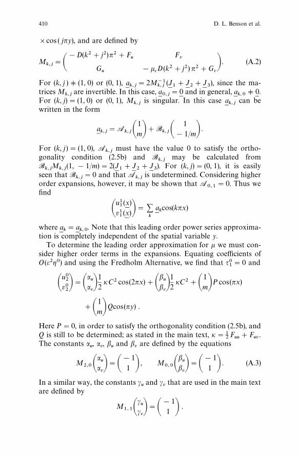
]cos ( jny), and are defined by

Mk,j

"A!D(k2#j2)n2#F

uFv

Gu

!kcD(k2#j2) n2#G

vB . (A.2)

For (k, j )9(1, 0) or (0, 1), ak, j

"2M~1k, j

(J1#J

2#J

3), since the ma-

trices Mk,j

are invertible. In this case, a0,j

"0 and in general, ak,0

90.For (k, j)"(1, 0) or (0, 1), M

k, jis singular. In this case a

k, jcan be

written in the form

ak,j

"Ak, jA

1mB#B

k, jA1

!1/mB .

For (k, j )"(1, 0), Ak, j

must have the value 0 to satisfy the ortho-gonality condition (2.5b) and B

k,jmay be calculated from

Bk,j

Mk, j

(1, !1/m)"2(J1#J

2#J

3). For (k, j)"(0, 1), it is easily

seen that Bk,j

"0 and that Ak,j

is undetermined. Considering higherorder expansions, however, it may be shown that A

0,1"0. Thus we

find

Au11(x)

v11(x)B"+

k

akcos(knx)

where ak"a

k,0. Note that this leading order power series approxima-

tion is completely independent of the spatial variable y.To determine the leading order approximation for k we must con-

sider higher order terms in the expansions. Equating coefficients ofO(e2g0) and using the Fredholm Alternative, we find that q0

1"0 and

Au02

v02B"A

au

avB12

iC2 cos(2nx)#Abu

bvB12

iC2#A1mBP cos(nx)

#A1mBQcos(ny) .

Here P"0, in order to satisfy the orthogonality condition (2.5b), andQ is still to be determined; as stated in the main text, i"1

2Fuu#F

uv.

The constants au, a

v, b

uand b

vare defined by the equations

M2,0A

au

avB"A

!11 B , M

0,0Abu

bvB"A

!11 B . (A.3)

In a similar way, the constants cuand c

vthat are used in the main text

are defined by

M1,1A

cu

cvB"A

!11 B .


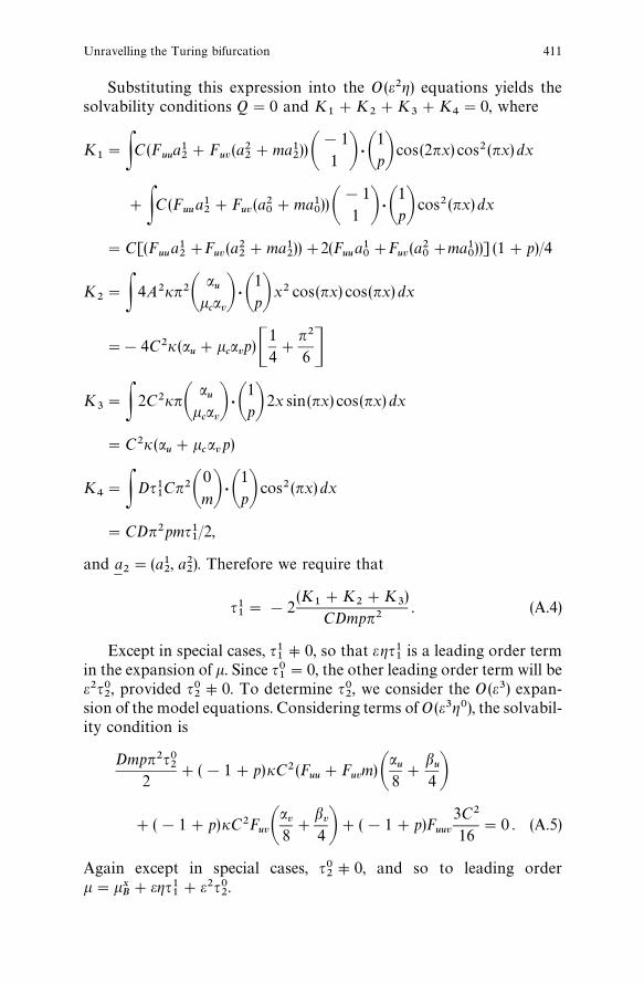
Substituting this expression into the O (e2g) equations yields thesolvability conditions Q"0 and K

1#K

2#K

3#K

4"0, where

K1"PC(F

uua12#F

uv(a2

2#ma1

2))A

!11 B · A

1pB cos(2nx) cos2(nx) dx

#PC (Fuu

a12#F

uv(a2

0#ma1

0))A

!11 B ·A

1pB cos2(nx) dx

"C[(Fuu

a12#F

uv(a2

2#ma1

2))#2(F

uua10#F

uv(a2

0#ma1

0))] (1#p)/4

K2"P 4A2in2A

au

kcavB · A

1pBx2 cos(nx) cos(nx) dx

"!4C2i(au#k

cavp)C

14#

n2

6 DK

3"P 2C2inA

au

kcavB ·A

1pB 2x sin(nx) cos(nx) dx

"C2i(au#k

cavp)

K4"P Dq1

1Cn2A

0mB ·A

1pB cos2(nx) dx

"CDn2pmq11/2,

and a2"(a1

2, a2

2). Therefore we require that

q11"!2

(K1#K

2#K

3)

CDmpn2. (A.4)

Except in special cases, q1190, so that egq1

1is a leading order term

in the expansion of k. Since q01"0, the other leading order term will be

e2q02, provided q0

290. To determine q0

2, we consider the O (e3) expan-

sion of the model equations. Considering terms of O(e3g0), the solvabil-ity condition is

Dmpn2q02

2#(!1#p)iC2(F

uu#F

uvm) A

au

8#

bu

4 B#(!1#p)iC2F

uvAav8#

bv

4 B#(!1#p)Fuuv

3C2

16"0 . (A.5)

Again except in special cases, q0290, and so to leading order

k"kxB#egq1

1#e2q0

2.


A1.2 The branch bifurcating at kyB

To approximate the solution near kyB, we observe, from equations (3.1)

and (3.4), that

Au01

v01B"A

1mBCcos(ny)

and (u11, v1

1) is a solution of the system

¸Au11

u11B"x2A

1kcmBCn2 cos(ny)#Dwy

1A0mBCn2 cos(ny) . (A.6)

Here the definition of wy1

given in (3.4b) guarantees the existence ofa solution to equation (A.6). Again, to determine this solution weexpress (u1

1, v1

1) as the Fourier cosine expansion

Au11

v11B" +

k,j|NAb1k, j

b2k, jB cos(knx) cos( jny)

and substitute this expression into equation (2.1). This gives rise toa series of linear equations for the b

j,kof the form

Mk, jA

b1k,j

b2k,jB cos(knx) cos( jny)"Dwy

1A0mBCn2 cos(ny)

#x2A1

kcmBCn2cos(ny) , (A.7)

where the matrices Mk,j

are defined by (A.2). For (k, j)9(0, 1) and(k, j)9(1, 0), the matrices M

k, jare invertible. In this case, (A.7) may be

solved for each bk, j

by multiplying each side of the equation bycos(knx)cos( jny) and integrating over the unit square. When j"1 andk90, we find that M

k, j(b1

k, j, b2

k, j)"(2C/k2)cos(kn) (1, k

cm), and when

j90 or 1 and k90, we find bj,k

"0. When (k, j)"(0, 1) or(k, j)"(1, 0), M

k, jis singular and we look for a solution of the form

Ab1k, j

b2k, jB"A

1mBA#A

1!1/mBB .

In the first case, A"0 by orthogonality but in general B is non-zeroand may be found by substitution. When (k, j)"(1, 0), it is obviousthat A"B"0. Thus we find

Au11(x)

v11(x)B"+

k

bk,1

cos(knx)cos(ny) .


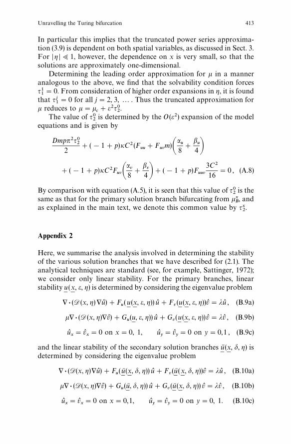
In particular this implies that the truncated power series approxima-tion (3.9) is dependent on both spatial variables, as discussed in Sect. 3.For D g D;1, however, the dependence on x is very small, so that thesolutions are approximately one-dimensional.

Determining the leading order approximation for k in a manneranalogous to the above, we find that the solvability condition forcesq11"0. From consideration of higher order expansions in g, it is found

that qj1"0 for all j"2, 3, 2 . Thus the truncated approximation for

k reduces to k"kc#e2q0

2.

The value of q02

is determined by the O (e2) expansion of the modelequations and is given by

Dmpn2q02

2#(!1#p)iC2(F

uu#F

uvm)A

au

8#

bu

4 B#(!1#p)iC2F

uvAav8#

bv

4 B#(!1#p)Fuuv

3C2

16"0 , (A.8)

By comparison with equation (A.5), it is seen that this value of q02

is thesame as that for the primary solution branch bifurcating from kx

B, and

as explained in the main text, we denote this common value by qx2.

Appendix 2

Here, we summarise the analysis involved in determining the stabilityof the various solution branches that we have described for (2.1). Theanalytical techniques are standard (see, for example, Sattinger, 1972);we consider only linear stability. For the primary branches, linearstability u (x, e, g) is determined by considering the eigenvalue problem

+ · (D (x, g)+uL )#Fu(u(x, e, g)) uL #F

v(u(x, e, g))vL"juL , (B.9a)

k+ · (D (x, g)+vL )#Gu(u, e, g)) uL #G

v(u (x, e, g))vL"jvL , (B.9b)

uLx"vL

x"0 on x"0, 1, uL

y"vL

y"0 on y"0,1 , (B.9c)

and the linear stability of the secondary solution branches uN (x, d, g) isdetermined by considering the eigenvalue problem

+ · (D(x, g)+uL )#Fu(uN (x, d, g)) uL #F

v(uN (x, d, g))vL"juL , (B.10a)

k+ · (D(x, g)+vL )#Gu(uN , d, g)) uL #G

v(uN (x, d, g)) vL"jvL , (B.10b)

uLx"vL

x"0 on x"0,1, uL

y"vL

y"0 on y"0, 1. (B.10c)


In both cases j represents the rate of linear growth of perturbationsuL (x) about the steady state solutions. In particular, the solution branchis stable if and only if j(0 for all perturbation solutions.

To solve the eigenvalue problem for j, we substitute the powerseries expansions for the primary and secondary solution branches intoequation (B.9) or (B.10) as appropriate, and assume that both j anduL (x) may be expressed as power series expansions in the same smallparameters. Thus on the primary solution branches, we look forsolutions of the eigenvalue problem of the form

uL (x, e, g)"euL1(x, g)#e2uL

2(x, g)#O(e3) (B.11a)

j(e, g)"j0(g)#ej

1(g)#e2j

2(g)#O(e3) , (B.11b)

satisfying DDuL1DD"1, where for i"1, 2, 2 and j"0, 1, 2, 2

uLi(x, g)"uL 0

i#guL 1

i#g2uL 2

i#O (g3)

jj(g)"j0

j#gj1

j#g2j2

j#O (g3) .

On the secondary solution branches, the appropriate power seriesexpansions are

uL (x, d, g)"duL1(x, g)#d2uL

2(x, g)#O(d3) (B.12a)

j(d, g)"j0(g)#dj

1(g)#d2j

2(g)#O (e3) , (B.12b)

satisfying DDuL1DD"1, where for i"1, 2, 2 and j"0, 1, 2, 2

uLi(g)"g1@2uL 1

i#guL 2

i#O(g3@2)

jj(g)"g1@2j1

j#gj2

j#O(g3@2) .

Substituting these expressions into the eigenvalue equations, the two-variable perturbation technique may then be used to determine theleading order approximation for j. Specifically, we approximate j onthe primary solution branches by

j"gj10#egj1

1#e2j0

2,

and on the secondary solution branches by

j"gj20#d2gj2

2.

From these approximations we are able to derive the conditions for thestability of the primary and secondary solution branches when g90and compare these with the conditions for the stability of primarystriped and spotted solutions when g"0 (see Sect. 5).

As this analysis is standard, we summarise the results for oursystem. Considering first the primary solution branch bifurcating fromkxB, we find that its stability for a given value of k, or equivalently for


a given value of the parameter e, is determined by the signs of jxand j

y,

where

jx"

Dn2mp1#mpGegq1

1#e22qx

2H (B.13)

jy"

Dn2mp1#mpG!g (wx

1!wy

1)#2e2(qxy

2!qx

2)H . (B.14)

When both jx(0 and j

y(0 the spatially inhomogeneous steady state

solution is stable; otherwise it is unstable. Equation (B.13) implies that

jx(08qx

2'0 and eN[e

L, 0] , (B.15)

where eL"!gq1

1/(2qx

2) is the position of the limit point denoted by

k"kL; for qx

2'0, the parameter interval [e

L, 0] corresponds to the

lower part of the subcritical region of the primary solution branch (seeFig. 1). Here we have used the fact that mp3(!1, 0) for all reactionkinetics which exhibit diffusion driven instability; this follows fromsimple algebraic manipulation of the equation (3.2) defining m and thecorresponding expression for p (given immediately before (3.4)). Sim-ilarly, we can deduce that

jy(08

(qxy2!qx

2)(0 and e2(e2

x,

(qxy2!qx

2)'0 and e2'e2

x,H if e2

x'0

jy(08(qxy

2!qx

2)'0 ∀e if e2

x(0,

where

ex"C

g (wx1!wy

1)

2(qxy2!qx

2)D

1@2

defines the position of the secondary bifurcation point kxS

when

wx1!wy

1qxy2!qx

2

'0 .

Thus, when kxS

exists, the primary solution branch is stable forkL(k(kx

Sif and only if qx

2'0, qx

2'qxy

2, and for k'kx

Sif and only if

qxy2'qx

2'0. When kx

Sdoes not exist, the solution branch is stable for

all k'kxB

whenever qxy2'qx

2'0. In particular, it follows that a neces-

sary condition for stability is qx2'0.

By a similar analysis, we may determine the stability conditions forthe primary solution branch bifurcating from ky

B; the results are out-

lined in Sect. 5.Using the above ideas we can also analyse the stability of the

solutions on the secondary branches. First we determine the stability ofthe secondary solution branch bifurcating from kx

S, which has power


series expansion (2.6). We find that the stability of the secondarysolution branch is determined by the signs of j

xand j

y, where

jx(d, g)"g

2Dn2mpqx2

1#mp!d2g

8Dmpn2qxy2

(qxy2!qx

2)

(1#mp)qx2

(B.16)

jy(dg)"!d2g

8Dmpn2qxy2

(qxy2!qx

2)

(1#mp)qx2

. (B.17)

The solutions are stable if both jx(0 and j

y(0, and are unstable

otherwise. It follows that for sufficiently small d, jx(08qx

2'0. As

before, we have used the fact that, for all parameter values lying inthe generalised Turing space, mp3(!1, 0). Similarly, j

y(08

qxy2

(qxy2!qx

2)/qx

2(0. Thus close to the secondary bifurcation point,

where d;1, there exist stable spotted solutions for k'kxSif and only if

qx2'qxy

2'0.

Acknowledgements. DLB was supported in part by a Wellcome Trust Prize Student-ship. Part of this work was carried out while PKM was visiting the Department ofMathematics, Williams College, Massachusettes. This work was supported in part bya grant from the London Mathematical Society.

References

Bauer, L., Keller, H. B. and Reiss, E. L., 1975, Multiple eigenvalues lead to secondarybifurcation. SIAM Review, 17, 101—122

Benson, D. L., Sherratt, J. A. and Maini, P. K., 1993, Diffusion driven instability in aninhomogeneous domain. Bull. Math. Biol., 55, 365—384

Boissonade, J., 1994, Long-range inhibition. Nature, 369, 188—189Borckmans, P., De Wit, A. and Dewel, G., 1992, Competition in ramped Turing

structures. Physica A, 188, 137—157De Wit, A., Dewel, G., Borckmans, P. and Walgraef, D., 1992, 3-Dimensional dissi-

pative structures in reaction diffusion-systems. Physica D, 61, 289—296Doedel, E., 1976, AUTO: software for continuation and bifurcation problems in

ordinary differential equations. Technical report, California Institute of TechnologyDufiet, V., and Boissonade, J., 1992a, Conventional and unconventional Turing

patterns. J. Chem. Phys., 96, 664—673Dufiet, V. and Boissonade, J., 1992b, Numerical studies of Turing pattern selection in

a two-dimensional system. Physica A, 118, 158—171Ermentrout, B., 1991, Stripes or spots? Nonlinear effects of bifurcation of reaction

diffusion equations on the square. Proc. R. Soc. Lond., A434, 413—417Gierer, A. and Meinhardt, H., 1972, A theory of biological pattern formation.

Kybernetik, 12, 30—39Hunding, A. and Br+ns, M., 1990, Bifurcation in a spherical reaction diffusion system

with imposed gradient. Physica D, 44, 285—302Iooss, G. and Joseph, D. D., 1980, Elementary stability and bifurcation theory, New

York: Springer-Verlag


Jenson, O., Pannbacker, V. O., Dewel, G. and Borckmans, P., 1993, Subcriticaltransitions to Turing structures. Phys. Lett. A, 179, 91—96

Lyons, M. J. and Harrison, L. G., 1991, A class of reaction diffusion models whichpreferentially select striped patterns. Chem. Phys. Lett., 183, 159—164

Lyons, M. J. and Harrison, L. G., 1992, Stripe selection: An intrinsic property of somepattern-forming models with non-linear dynamics. Devel. Dyn., 195, 201—215

Mahar, T. J. and Matkowsky, B. J., 1977, A model biochemical reaction exhibitingsecondary bifurcation. SIAM Review, 32, 394—404

Malomed, B. A. and Tribel’skii, M. I., 1987, Stability of stationary periodic structuresfor weakly supercritical convection and in related problems. Sov. Phys. JETP, 65,305—310

Maini, P. K., Benson, D. L. and Sherratt, J. A., 1992, Pattern formation in reaction-diffusion models with spatially inhomogeneous diffusion coefficients. IMA J. Math.Appl. Med. Biol., 9, 197—213

Maini, P. K., Myerscough, M. R., Winters, K. H. and Murray, J. D., 1991, Bifurcatingspatially heterogeneous solutions in a chemotaxis model for biological patterngeneration. Bull. Math. Biol., 53, 701—719

Meinhardt, H., 1993, A model for pattern formation of hypostome, tentacles, andfoot in hydra — how to form structures close to each other, how to form them ata distance. Dev. Biol., 157, 321—333

Murray, J. D., 1981, A pre-pattern formation mechanism for animal coat markings.J. theor. Biol., 88, 161—199

Murray, J. D., 1982, Parameter space for Turing instability in reaction diffusionmechanisms: A comparison of models. J. theor. Biol., 98, 143—163

Murray, J. D., 1989, Mathematical Biology. Heidelberg: Springer-VerlagNagorcka, B. N., 1995a, The reaction-diffusion theory of wool (hair) follicle initiation

and development. 1. primary follicles. Austr. J. Agric. Res., 46, 333—355Nagorcka, B. N., 1995b, The reaction-diffusion theory of wool (hair) follicle initiation

and development. 2. original secondary follicles. Austr. J. Agric. Res., 46, 357—378Perraud, J. J., De Wit, A., De Kepper, P., Dewel G. and Borckmans, P., 1993, One-

dimensional spirals; Novel asynchronous chemical waves sources. Phys. Rev. Lett.,71, 1272—1275

Reiss, E. L., 1983, Cascading bifurcations. SIAM J. Appl. Math., 43, 57—65Sattinger, D. H., 1972, Six lectures on the transition to instability. In Lecture Notes in

Mathematics, 322, Berlin: Springer—VerlagSchnakenberg, J., 1979, Simple chemical reaction systems with limit cycle behaviour.

J. Theor. Biol., 81, 389—400Segel, L. A. and Jackson, J. L., 1972, Dissipative structure: an explanation and an

ecological example. J. Theor. Biol., 37, 545—559Sherratt, J. A., 1995, Turing bifurcations with a temporally varying diffusion coeffic-

ient. J. Math. Biol., 33, 295—308Turing, A. M., 1952, The chemical basis of morphogenesis. Phil. Trans. R. Soc. Lond.,

B237, 37—72


Unravelling the Turing bifurcation using spatially varying ... · Unravelling the Turing...

Documents

Transcript of Unravelling the Turing bifurcation using spatially varying ... · Unravelling the Turing...