Unmixing methodsbased onnonnegativity and weakly mixed
28
Astronomy & Astrophysics manuscript no. Hershel˙BSS © ESO 2020 November 20, 2020 Unmixing methods based on nonnegativity and weakly mixed pixels for astronomical hyperspectral datasets A. Boulais, O. Bern´ e, G. Faury, and Y. Deville IRAP, Universit´ e de Toulouse, UPS, CNRS, CNES, 9 Av. colonel Roche, BP 44346, F-31028 Toulouse cedex 4, France Received ??? ; accepted ??? ABSTRACT An increasing number of astronomical instruments (on Earth and space-based) provide hyperspectral images, that is three-dimensional data cubes with two spatial dimensions and one spectral dimension. The intrinsic limitation in spatial resolution of these instruments implies that the spectra associated with pixels of such images are most often mixtures of the spectra of the “pure” components that exist in the considered region. In order to estimate the spectra and spatial abundances of these pure components, we here propose an original blind signal separation (BSS), that is to say an unsupervised unmixing method. Our approach is based on extensions and combinations of linear BSS methods that belong to two major classes of methods, namely nonnegative matrix factorization (NMF) and Sparse Component Analysis (SCA). The former performs the decomposition of hyperspectral images, as a set of pure spectra and abundance maps, by using nonnegativity constraints, but the estimated solution is not unique: It highly depends on the initialization of the algorithm. The considered SCA methods are based on the assumption of the existence of points or tiny spatial zones where only one source is active (i.e., one pure component is present). These points or zones are then used to estimate the mixture and perform the decomposition. In real conditions, the assumption of perfect single-source points or zones is not always realistic. In such conditions, SCA yields approximate versions of the unknown sources and mixing coefficients. We propose to use part of these preliminary estimates from the SCA to initialize several runs of the NMF in order to refine these estimates and further constrain the convergence of the NMF algorithm. The proposed methods also estimate the number of pure components involved in the data and they provide error bars associated with the obtained solution. Detailed tests with synthetic data show that the decomposition achieved with such hybrid methods is nearly unique and provides good performance, illustrating the potential of applications to real data. Key words. astrochemistry - ISM: molecules - molecular processes - Methods: numerical 1. Introduction Telescopes keep growing in diameter, and detectors are more and more sensitive and made up of an increasing number of pixels. Hence, the number of photons that can be captured by astronomical instruments, in a given amount of time and at a given wavelength, has increased significantly, thus allowing as- tronomy to go hyperspectral. More and more, astronomers do not deal with 2D images or 1D spectra, but with a combination of these media resulting in three-dimensional (3D) data cubes (two spatial dimensions, one spectral dimension). We hereafter provide an overview of the instruments that provide hyperspec- tral data in astronomy, mentioning specific examples without any objective to be exhaustive. Several integral field unit spectro- graphs (e.g., MUSE on the Very Large Telescope) provide spec- tral cubes at visible wavelengths, yielding access to the optical tracers of ionized gas (see for instance Weilbacher et al. 2015). Infrared missions such as the Infrared Space Observatory (ISO) and Spitzer performed spectral mapping in the mid-infrared, a domain that is particularly suited to observe the emission of UV heated polycyclic aromatic hydrocarbon (e.g., Cesarsky et al. 1996; Werner et al. 2004). In the millimeter wavelengths, large spectral maps in rotational lines of abundant molecules (typi- cally CO) have been used for several decades to trace the dy- namics of molecular clouds (e.g., Bally et al. (1987); Miesch & Bally (1994); Falgarone et al. (2009)). The PACS, SPIRE, and HIFI instruments, on board Herschel all have a mode that al- lows for spectral mapping (e.g. Van Kempen et al. 2010; Habart et al. 2010; Joblin et al. 2010) in atomic and molecular lines. Owing to its high spectral resolution, HIFI allows one to resolve the profiles of these lines, enabling one to study the kinemat- ics of, for example, the immediate surroundings of protostars (Kristensen et al. (2011)) or of star-forming regions (Pilleri et al. (2012)) using radiative transfer models. Similarly, the GREAT instrument on board the Stratospheric Observatory For Infrared Astronomy (SOFIA) now provides large-scale spectral maps in the C + line at 1.9 THz (Pabst et al. (2017)). The Atacama Large Millimeter Array (ALMA) also provides final products that are spectral cubes (see e.g., Goicoechea et al. (2016)). A majority of astronomical spectrographs to be employed at large observato- ries in the future will provide spectral maps. This is the case for the MIRI and NISPEC instruments on the James Webb Space Telescope (JWST) and the METIS instrument on the Extremely Large Telescope (ELT). Although such 3D datasets have become common, few meth- ods have been developed by astronomers to analyze the outstand- ing amount of information they contain. Classical analysis meth- ods tend to decompose the spectra by fitting them with simple functions (typically mixtures of Gaussians) but this has several disadvantages: 1) the a priori assumption made by the use of a given function is usually not founded physically, 2) if the num- ber of parameters is high, the result of the fit may be degener- ate, 3) for large datasets and fitting with nonlinear functions, the fitting may be very time consuming, 4) initial guesses must be provided, and, 5) the spectral fitting is usually performed on a (spatial) pixel by pixel basis, so that the extracted components 1 arXiv:2011.09742v1 [astro-ph.IM] 19 Nov 2020
Transcript of Unmixing methodsbased onnonnegativity and weakly mixed

Astronomy & Astrophysics manuscript no. Hershel˙BSS © ESO 2020November 20, 2020
Unmixing methods based on nonnegativity and weakly mixedpixels for astronomical hyperspectral datasets
A. Boulais, O. Berne, G. Faury, and Y. Deville
IRAP, Universite de Toulouse, UPS, CNRS, CNES,9 Av. colonel Roche, BP 44346, F-31028 Toulouse cedex 4, France
Received ??? ; accepted ???
ABSTRACT
An increasing number of astronomical instruments (on Earth and space-based) provide hyperspectral images, that is three-dimensionaldata cubes with two spatial dimensions and one spectral dimension. The intrinsic limitation in spatial resolution of these instrumentsimplies that the spectra associated with pixels of such images are most often mixtures of the spectra of the “pure” components thatexist in the considered region. In order to estimate the spectra and spatial abundances of these pure components, we here proposean original blind signal separation (BSS), that is to say an unsupervised unmixing method. Our approach is based on extensions andcombinations of linear BSS methods that belong to two major classes of methods, namely nonnegative matrix factorization (NMF)and Sparse Component Analysis (SCA). The former performs the decomposition of hyperspectral images, as a set of pure spectra andabundance maps, by using nonnegativity constraints, but the estimated solution is not unique: It highly depends on the initializationof the algorithm. The considered SCA methods are based on the assumption of the existence of points or tiny spatial zones whereonly one source is active (i.e., one pure component is present). These points or zones are then used to estimate the mixture andperform the decomposition. In real conditions, the assumption of perfect single-source points or zones is not always realistic. Insuch conditions, SCA yields approximate versions of the unknown sources and mixing coefficients. We propose to use part of thesepreliminary estimates from the SCA to initialize several runs of the NMF in order to refine these estimates and further constrain theconvergence of the NMF algorithm. The proposed methods also estimate the number of pure components involved in the data andthey provide error bars associated with the obtained solution. Detailed tests with synthetic data show that the decomposition achievedwith such hybrid methods is nearly unique and provides good performance, illustrating the potential of applications to real data.
Key words. astrochemistry - ISM: molecules - molecular processes - Methods: numerical
1. Introduction
Telescopes keep growing in diameter, and detectors are moreand more sensitive and made up of an increasing number ofpixels. Hence, the number of photons that can be captured byastronomical instruments, in a given amount of time and at agiven wavelength, has increased significantly, thus allowing as-tronomy to go hyperspectral. More and more, astronomers donot deal with 2D images or 1D spectra, but with a combinationof these media resulting in three-dimensional (3D) data cubes(two spatial dimensions, one spectral dimension). We hereafterprovide an overview of the instruments that provide hyperspec-tral data in astronomy, mentioning specific examples without anyobjective to be exhaustive. Several integral field unit spectro-graphs (e.g., MUSE on the Very Large Telescope) provide spec-tral cubes at visible wavelengths, yielding access to the opticaltracers of ionized gas (see for instance Weilbacher et al. 2015).Infrared missions such as the Infrared Space Observatory (ISO)and Spitzer performed spectral mapping in the mid-infrared, adomain that is particularly suited to observe the emission of UVheated polycyclic aromatic hydrocarbon (e.g., Cesarsky et al.1996; Werner et al. 2004). In the millimeter wavelengths, largespectral maps in rotational lines of abundant molecules (typi-cally CO) have been used for several decades to trace the dy-namics of molecular clouds (e.g., Bally et al. (1987); Miesch &Bally (1994); Falgarone et al. (2009)). The PACS, SPIRE, andHIFI instruments, on board Herschel all have a mode that al-lows for spectral mapping (e.g. Van Kempen et al. 2010; Habart
et al. 2010; Joblin et al. 2010) in atomic and molecular lines.Owing to its high spectral resolution, HIFI allows one to resolvethe profiles of these lines, enabling one to study the kinemat-ics of, for example, the immediate surroundings of protostars(Kristensen et al. (2011)) or of star-forming regions (Pilleri et al.(2012)) using radiative transfer models. Similarly, the GREATinstrument on board the Stratospheric Observatory For InfraredAstronomy (SOFIA) now provides large-scale spectral maps inthe C+ line at 1.9 THz (Pabst et al. (2017)). The Atacama LargeMillimeter Array (ALMA) also provides final products that arespectral cubes (see e.g., Goicoechea et al. (2016)). A majority ofastronomical spectrographs to be employed at large observato-ries in the future will provide spectral maps. This is the case forthe MIRI and NISPEC instruments on the James Webb SpaceTelescope (JWST) and the METIS instrument on the ExtremelyLarge Telescope (ELT).
Although such 3D datasets have become common, few meth-ods have been developed by astronomers to analyze the outstand-ing amount of information they contain. Classical analysis meth-ods tend to decompose the spectra by fitting them with simplefunctions (typically mixtures of Gaussians) but this has severaldisadvantages: 1) the a priori assumption made by the use of agiven function is usually not founded physically, 2) if the num-ber of parameters is high, the result of the fit may be degener-ate, 3) for large datasets and fitting with nonlinear functions, thefitting may be very time consuming, 4) initial guesses must beprovided, and, 5) the spectral fitting is usually performed on a(spatial) pixel by pixel basis, so that the extracted components
1
arX
iv:2
011.
0974
2v1
[as
tro-
ph.I
M]
19
Nov
202
0

A. Boulais, O. Berne, G. Faury, and Y. Deville: Unmixing methods for astronomical hyperspectral datasets
are spatially independent, whereas physical components are of-ten present at large scales on the image. An alternative is to an-alyze the data by means of principal component analysis (e.g.,Neufeld et al. 2007; Gratier et al. 2017), which provides a rep-resentation of the data in an orthogonal basis of a subspace, thusallowing interpretation. However, this may be limited by the factthat the principal components are orthogonal, and hence they arenot easily interpretable in physical terms. An alternative analysiswas proposed by Juvela et al. (1996), which is based on a BlindSignal Separation (BSS) approach. It consists in decomposingspectral cubes (in their case, CO spectral maps) into the productof a small number of spectral components, or “end members”,and spatial “abundance” maps.
This requires no a priori on spectral properties of the compo-nents, and hence this can provide deeper insights into the physi-cal structure represented in the data, as demonstrated in this pi-oneering paper. This method uses the positivity constraint forthe maps and spectra (all their points must be positive) com-bined with the minimization of a statistical criterion to derivethe maps and spectral components. This method is referred to aspositive matrix factorization (PMF, Paatero & Tapper (1994)).Although it contained the original idea of using positivity as aconstraint to estimate a matrix product, this work used a classicaloptimization algorithm. Several years later, Lee & Seung (1999)introduced a novel algorithm to perform PMF using simple mul-tiplicative iterative rules, making the PMF algorithm extremelyfast. This algorithm is usually referred to as Lee and Seung’sNon Negative Matrix Factorization (NMF hereafter) and hasbeen widely used in a vast number of applications outside as-tronomy. This algorithm has proved to be efficient including inastrophysical applications (Berne et al. 2007). However, NMFhas several disadvantages: 1) the number of spectra to be ex-tracted must be given by the user, 2) the error bars related tothe procedure are not derived automatically, 3) convergence to aunique point is not guaranteed and may depend on initialization(see Donoho & Stodden 2003 on these latter aspects). When ap-plying NMF to astronomical hyperspectral data, the above draw-backs become critical and can jeopardize the integrity of the re-sults.
In this paper, we evaluate possibilities to improve applica-tion of BSS to hyperspectral positive data by hybridizing NMFwith sparsity-based algorithms. Here, we focus on syntheticdata, so as to perform a detailed comparison of the performancesof the proposed approaches. A first application on real data ofone of the methods presented here is provided in Foschino et al.(2019). The proposed methods should be applicable to any hy-perspectral dataset fulfilling the properties that we will describehereafter. The paper is organized as follows. In the next sec-tion we present the adopted mathematical model for hyperspec-tral astronomical data, using tow possible conventions, spatialor spectral. We describe the mixing model and associated “blindsignal separation” (BSS) problem. In Section 3, we describe thepreliminary steps (preprocessing steps) that are required beforeapplying the proposed algorithms. In Section 4 we describe indetails the three methods that are used in this paper, that is, NMF(with an extension using a Monte-Carlo approach referred to asMC-NMF) and two methods based on sparsity (Space-CORRand Maximum Angle Source Separation, MASS). We then detailhow MC-NMF can be hybridized with the latter two methods.
In Section 5, a comparative performance analysis of studiedmethods is performed. We conclude in Section 6.
Table 1. List of major variables
Variable Descriptionspec(l, v) Value of elementary spectrum l at velocity index v
S pec Matrix of values spec(l, v) of elementary spectramap(m, l) Scale factor of elementary spectrum p in pixel m
Map Matrix of scale factors map(m, l)obs(m, v) Observed value of pixel m at velocity v
Obs Matrix of observed values obs(m, v)
2. Data model and blind source separation problem
The observed data consist of a spectral cube C(px, py, f ) of di-mension Px×Py×N where (px, py) define the spatial coordinatesand f is the spectral index. To help one interpret the results, thespectral index is hereafter expressed as a Doppler-shift velocityin km/s, using v = c× ( f − f0)/ f0, with f the observed frequency,f0 the emitted frequency and c the light speed. We assume thatall observed values in C are nonnegative. We call each vectorC(px, py, .) recorded at a position (px, py) “spectrum” and wecall each matrix C(., ., v) recorded at a given velocity “spectralband.” Each observed spectrum corresponding to a given pixelresults from a mixture of different kinematic components that arepresent on the line of sight of the instrument. Mathematically,the observed spectrum obtained for one pixel is then a combina-tion (which will be assumed to be linear and instantaneous) ofelementary spectra.
In order to recover these elementary spectra, one can usemethods known as Blind Source Separation (BSS). BSS con-sists in estimating a set of unknown source signals from a set ofobserved signals that are mixtures of these source signals. Thelinear mixing coefficients are unknown and are also to be esti-mated. The observed spectral cube is then decomposed as a setof elementary spectra and a set of abundance maps (the contri-butions of elementary spectra in each pixel).
Considering BSS terminology and a linear mixing model, thematrix containing all observations is expressed as the product ofa mixing matrix and a source matrix. Therefore, it is necessaryhere to restructure the hyperspectral cube C into a matrix and toidentify what we call “observations”, “samples”, “mixing coef-ficients”, and “sources”. A spectral cube can be modeled in twodifferent ways: a spectral model where we consider the cube asa set of spectra and a spatial model where we consider the cubeas a set of images (spectral bands), as detailed hereafter.
2.1. Spectral model
For the spectral data model, we define the observations as beingthe spectra C(px, py, .). The data cube C is reshaped into a newmatrix of observations Obs (variables defined in this section aresummarized in Table 1), where the rows contain the Px × Py =M observed spectra of C arranged in any order and indexed bym. Each column of Obs corresponds to a given spectral samplewith an integer-valued index also denoted as v ∈ 1, . . . ,N forall observations. Each observed spectrum obs(m, .) is a linearcombination of L (L M) unknown elementary spectra andyields a different mixture of the same elementary spectra:
obs(m, v) =
L∑`=1
map(m, `) spec(`, v) (1)
m ∈ 1, . . . ,M, v ∈ 1, . . . ,N, ` ∈ 1, . . . , L,
2

A. Boulais, O. Berne, G. Faury, and Y. Deville: Unmixing methods for astronomical hyperspectral datasets
where obs(m, v) is the vth sample of the mth observation,spec(`, v) is the vth sample of the `th elementary spectrum andmap(m, `) defines the contribution scale of elementary spectrum` in observation m. Using the BSS terminology, map stands forthe mixing coefficients and spec stands for the sources. Thismodel can be rewritten in matrix form:
Obs = Map × S pec, (2)
where Map is an M × L mixing matrix and S pec is an L × Nsource matrix.
2.2. Spatial model
For the spatial data model, we define the observations as be-ing the spectral bands C(., ., v). The construction of the spatialmodel is performed by transposing the spectral model (2). Inthis configuration, the rows of the observation matrix ObsT (thetranspose of the original matrix of observations Obs) containthe N spectral bands with a one-dimensional structure. Eachcolumn of ObsT corresponds to a given spatial sample indexm ∈ 1, . . . ,M for all observations (i.e., each column corre-sponds to a pixel). Each spectral band ObsT (v, .) is a linear com-bination of L (L N) unknown abundance maps and yields adifferent mixture of the same abundance maps:
ObsT = S pecT × MapT , (3)
where ObsT is the transpose of the original observation matrix,S pecT is the N ×L mixing matrix and MapT is the L×M sourcematrix. In this alternative data model, the elementary spectra inS pecT stand for the mixing coefficients and the abundance mapsin MapT stand for the sources.
2.3. Problem statement
In this section, we denote the mixing matrix as A and the sourcematrix as S , whatever the nature of the adopted model (spatialor spectral) to simplify notations, the following remarks beingvalid in both cases.
The goal of BSS methods is to find estimates of a mixingmatrix A and a source matrix S , respectively denoted as A andS , and such that:
X ≈ AS . (4)
However this problem is ill-posed. Indeed, if A, S is a solu-tion, then AP−1, PS is also a solution for any invertible ma-trix P. To achieve the decomposition, we must add two extraconstraints. The first one is a constraint on the properties of theunknown matrices A and/or S . The type of constraint (indepen-dence of sources, nonnegative matrices, sparsity) leads directlyto the class of methods that will be used for the decomposition.The case of linear instantaneous mixtures was first studied in the1980s, then three classes of methods became important:
– Independent component analysis (ICA) (Cardoso (1998);Hyvarinen et al. (2001)): It is based on a probabilistic for-malism and requires the source signals to be mutually statis-tically independent. Until the early 2000s, ICA was the onlyclass of methods available to achieve BSS.
– Nonnegative matrix factorization (NMF) (Lee & Seung(1999)): It requires the source signals and mixing coefficientsvalues to be nonnegative.
– Sparse component analysis (SCA) (Gribonval & Lesage(2006)): It requires the source signals to be sparse in the con-sidered representation domain (time, time-frequency, time-scale, wavelet...).
The second constraint is to determine the dimensions ofA and S . Two of these dimensions are obtained directly fromobservations X (M and N). The third dimension, common toboth A and S matrices, is the number of sources L, which mustbe estimated.
Here, we consider astrophysical hyperspectral data that havethe properties listed below. These are relatively general proper-ties that are applicable to a number of cases with Herschel-HIFI,ALMA, Spitzer, JWST, etc:
– They do not satisfy the condition of independence of thesources. In our simulated data, elementary spectra have, byconstruction, similar variations (Gaussian spectra with dif-ferent means, see Section 5.1). Likewise, abundance mapsassociated with each elementary spectrum have similarshapes. Such data involve nonzero correlation coefficientsbetween elementary spectra and between abundance maps.Hence ICA methods will not be discussed in this paper.
– These data are nonnegative if we disregard noise. Each pixelprovides an emission spectrum, hence composed of positiveor zero values. Such data thus correspond to the conditionsof use of NMF that we detail in Section 4.1.
– If we consider the data in a spatial framework (spatialmodel), the cube provides a set of images. We can then for-mulate the hypothesis that there are regions in these imageswhere only one source is present. This is detailed in Section4.2. This hypothesis then refers to a “sparsity” assumption inthe data and SCA methods are then applicable to hyperspec-tral cubes. On the contrary, sparsity properties do not exist inthe spectral framework in our case, as discussed below.
– If the data have some sparsity properties, adding the non-negativity assumption enables the use of geometric methods.The geometric methods are a subclass of BSS methods basedon the identification of the convex hull containing the mixeddata. However, the majority of geometric methods, whichare used in hyperspectral unmixing in Earth observation, arenot applicable to Astrophysics because they set an additionalconstraint on the data model: they require all abundance co-efficients to sum to one in each pixel, which changes thegeometrical representation of the mixed data. On the con-trary, in Section 4.3, we introduce a geometric method calledMASS, for Maximum Angle Source Separation (Boulaiset al. (2015)), which may be used in an astrophysical con-text (i.e., for data respecting the models presented above).
The sparsity constraint required for SCA and geometricmethods is carried by the source matrix S . These methods maytherefore potentially be applied in two ways to the above-defineddata: either we suppose that there exist spectral indices for whicha unique spectral source is nonzero, or we suppose that there ex-ist some regions in the image for which a unique spatial sourceis zero. In our context of studying the properties of photodisso-ciation regions, only the second case is realistic. Thus only themixing model (3) is relevant. Therefore, throughout the rest ofthis paper, we will only use that spatial data model (3), so thatwe here define the associated final notations and vocabulary: letX = ObsT be the (N × M) observation matrix, A = S pecT the(N × L) mixing matrix containing the elementary spectra andS = MapT the (L × M) source matrix containing the spatialabundance maps, each associated with an elementary spectrum.
Moreover, we note that in the case of the NMF, the spectraland spatial models are equivalent but the community generallyprefers the more intuitive spectral model.
3

A. Boulais, O. Berne, G. Faury, and Y. Deville: Unmixing methods for astronomical hyperspectral datasets
Before thoroughly describing the algorithms used for theaforementioned BSS methods, we present preprocessing stagesrequired for the decomposition of data cubes.
3. Data preprocessing
3.1. Estimation of number of sources
An inherent problem in BSS is to estimate the number L ofsources (the dimension shared by the A and S matrices). Thisparameter should be fixed before performing the decomposi-tion in the majority of cases. Here, this estimate is based on theeigen-decomposition of the covariance matrix of the data. As inPrincipal Component Analysis (PCA), we look for the minimumnumber of components that most contribute to the total varianceof the data. Thus the number of high eigenvalues is the numberof sources in the data. Let ΣX be the (N × N) covariance matrixof observations X:
ΣX =1M
XcXTc =
N∑i=1
λieieTi , (5)
where λi is the ith eigenvalue associated with eigenvector ei andXc is the matrix of centered data (i.e. each observation has zeromean: xc(n, .) = x(n, .) − x(n, .) ).
The eigenvalues of ΣX have the following properties (theirproofs are available in Deville et al. (2014)):
Property 1: For noiseless data (X0 = AS ), the ΣX matrixhas L positive eigenvalues and N − L eigenvalues equal to zero.
The number L of sources is therefore simply inferred fromthis property. Now, we consider the data with an additive spa-tially white noise E, with standard deviation σE , i.e., X = X0+E.The relation between the covariance matrix ΣX0 of noiseless dataand the covariance matrix ΣX of noisy data is then:
ΣX = ΣX0 + σ2E IN , (6)
where IN is the identity matrix.
Property 2: The eigenvalues λ of ΣX and the eigenvalues λ0of ΣX0 are linked by:
λ = λ0 + σ2E . (7)
These two properties then show that the ordered eigenvalues λ(i)of ΣX for a mixture of L sources are such that:
λ(1) ≥ . . . ≥ λ(L) > λ(L+1) = . . . = λ(N) = σ2E . (8)
But in practice, because of the limited number of samples andsince the strong assumption of a white noise with the same stan-dard deviation in all pixels is not fulfilled, the equality λ(L+1) =
. . . = λ(N) = σ2E is not met. However, the differences between
the eigenvalues λ(L+1), . . . , λ(N) are small compared to the dif-ferences between the eigenvalues λ(1), . . . , λ(L). The curve of theordered eigenvalues is therefore constituted of two parts. Thefirst part, ΩS , contains the first L eigenvalues associated with astrong contribution in the total variance. In this part, eigenval-ues are significantly different. The second part, ΩE , contains theother eigenvalues, associated with noise. In this part, eigenvaluesare similar.
The aim is then to identify from which rank r = L + 1 eigen-values no longer vary significantly. To this end, we use a method
based on the gradient of the curve of ordered eigenvalues (Luo& Zhang (2000)) in order to identify a break in this curve (seeFig. 5).
Moreover, a precaution must be taken concerning the differ-ence between λ(L) and λ(L+1). In simulations, we found that in thenoiseless case, it is possible that the last eigenvalues of ΩS areclose to zero. Thus, for very noisy mixtures, the differences be-tween these eigenvalues become negligible relative to the noisevariance σ2
E . These eigenvalues are then associated with ΩE andtherefore rank r where a “break” appears will be underestimated.
The procedure described by Luo & Zhang (2000) is as fol-lows:
1. Compute the eigen-decomposition of the covariance matrixΣX and arrange the eigenvalues in decreasing order.
2. Compute the gradient of the curve of the logarithm of the Lfirst (typically L = 20) ordered eigenvalues:
∇λ(i) = ln(λ(i)/λ(i+1)) i ∈ 1, . . . , L. (9)
3. Compute the average gradient of all these eigenvalues:
∇λ =1
(L − 1)ln(λ(1)/λ(L)). (10)
4. Find all i satisfying ∇λ(i) < ∇λ to construct the set I =
i | ∇λ(i) < ∇λ.5. Select the index r, such that it is the first one of the last con-
tinuous block of i in the set I.6. The number of sources is then L = r − 1.
3.2. Noise reduction
The observed spectra are contaminated by noise. In syntheticdata, this noise is added assuming it is white and Gaussian. Noisein real data may have different properties, however the aforemen-tioned assumptions are made here in order to evaluate the sen-sitivity of the method to noise in the general case. To improvethe performance of the above BSS methods, we propose differ-ent preprocessing stages to reduce the influence of noise on theresults.
The first preprocessing stage consists of applying a spectralthresholding, i.e., only the continuous range of v containing sig-nal is preserved. Typically many first and last channels containonly noise and are therefore unnecessary for the BSS. This isdone for all BSS methods presented in the next section.
The second preprocessing stage consists of applying a spatialthresholding. Here, we must distinguish the case of each BSSmethod because the SCA method requires to retain the spatialstructure of data. For NMF, the observed spectra (columns of X)whose “normalized power” is lower than a threshold αe are dis-carded. Typically some spectra contain only noise and are there-fore unnecessary for the spectra estimation step (Section 4.1).In our application, we set the threshold to αe = max
i‖X(., i)‖ ×
0.2 (∀i ∈ 1, . . . ,M). For the SCA method, some definitions arenecessary to describe this spatial thresholding step. This proce-dure is therefore presented in the section regarding the methoditself (Section 4.2).
Finally, synthetic and actual data from the HIFI instrumentcontain some negative values due to noise. To stay in the as-sumption of NMF, these values are reset to ε = 10−16.
4

A. Boulais, O. Berne, G. Faury, and Y. Deville: Unmixing methods for astronomical hyperspectral datasets
4. Blind signal separation methods
4.1. nonnegative matrix factorization and our extension
NMF is a class of methods introduced by Lee & Seung (1999).The standard algorithm iteratively and simultaneously computesA and S , minimizing an objective function of the initial X matrixand the AS product. In our case, we use the minimization of theEuclidean distance δ = 1
2‖X − AS ‖2F , using multiplicative updaterules:
A← A (XS T ) (AS S T ) (11)
S ← S (AT X) (AT AS ), (12)
where and are respectively the element-wise product anddivision.
Lee and Seung show that the Euclidean distance δ is non in-creasing under these update rules (Lee & Seung (2001)), so thatstarting from random A and S matrices, the algorithm will con-verge toward a minimum for δ. We estimate that the convergenceis reached when:
1 −δi+1
δi < κ, (13)
where i corresponds to the iteration and κ is a threshold typicallyset to 10−4.
The main drawback of standard NMF is the uniqueness ofthe decomposition. The algorithm is sensitive to the initializationdue to the existence of local minima of the objective function(Cichocki et al. (2009)). The convergence point highly dependson the distance between the initial point and a global minimum.A random initialization without additional constraint is generallynot satisfactory. To improve the quality of the decomposition,several solutions are possible:
– Use a Monte-Carlo analysis to estimate the elementaryspectra and then rebuild the abundance maps (Berne et al.(2012)).
– Further constrain the convergence by altering the initializa-tion (Langville et al. (2006)).
– Use additional constraints on the sources and/or mixing coef-ficients, such as sparsity constraints (Cichocki et al. (2009)),or geometric constraints (Miao & Qi (2007)).
The addition of geometric constraints is usually based onthe sum-to-one of the abundance coefficients for each pixel
(L∑=1
sm(`) = 1). This condition is not realistic in an astrophysi-
cal context, where the total power received by the detectors varyfrom a pixel to another. Therefore, this type of constraints cannotbe applied here. A standard type of sparsity constraints imposesa sparse representation of the estimated matrices A and/or S inthe following sense: the spectra and/or the abundance maps havea large number of coefficients equal to zero or negligible. Onceagain, this property is not verified in the data that we considerand so this type of constraint cannot be applied. However, theabove type of sparsity must be distinguished from the sparsityproperties exploited in the SCA methods used in this paper. Thisis discussed in Sections 4.2 and 4.3 dedicated to these methods.
Moreover, well-known indeterminacies of BSS appear in theA and S estimated matrices. The first one is a possible permuta-tion of sources in S . The second one is the presence of a scalefactor per estimated source. To offset these scale factors, the es-timated source spectra are normalized so that:∫
a`(v) dv = 1 ` ∈ 1, . . . , L (14)
where a` is the `th column of A. This normalization allows theabundance maps to be expressed in physical units.
To improve the results of standard NMF, we extend it as fol-lows. First, the NMF is amended to take into account the nor-malization constraint (14). At each iteration (i.e. each updateof A according to (11)), the spectra are normalized in order toavoid the scale indeterminacies. Then NMF is complemented bya Monte-Carlo analysis described hereafter. Finally, we proposean alternative to initialize NMF with results from one of the SCAmethods described in Sections 4.2 and 4.3.
The NMF-based method used here (called MC-NMF here-after), combining standard NMF, normalization and Monte-Carlo analysis, has the following structure:
– The Monte-Carlo analysis stage gives the most probablesamples of elementary spectra and error bars associated withthese estimates provided by the normalized NMF.
– The combination stage recovers abundance map sourcesfrom the above estimated elementary spectra and observa-tions.
These two stages are described hereafter:
1. Monte-Carlo analysis: Assuming that the number of sourcesL is known (refer to Section 3.1 for its estimation), NMF is ranp times, with different initial random matrices for each trial (p istypically equal to 100). In each run, a set of L elementary spectraare identified. The total number of obtained spectra at the end ofthis process is p × L. These spectra are then grouped into L setsω1, ω2, . . . , ωL, each set representing the same column of A.To achieve this clustering, the method uses the K-means algo-rithm (Theodoridis & Koutroumbas (2009)) with a correlationcriterion, provided in Matlab (kmeans). More details about theK-means algorithm are provided in Appendix A.
To then derive the estimated value a`(v) of each elementaryspectrum, at each velocity v in a set ω`, we estimate the proba-bility density function (pdf) fω` ,v from the available p intensitieswith the Parzen kernel method provided in Matlab (ksdensity).Parzen kernel (Theodoridis & Koutroumbas (2009)) is a para-metric method to estimate the pdf of a random variable at anypoint of its support. For more details about this method, refer toAppendix A.
Each estimated elementary spectrum a` is obtained by se-lecting the intensity u that has the highest probability at a givenwavelength:
a`(v) = argmaxu
fω` ,v(u) ` ∈ 1, . . . , L. (15)
The estimation error at each wavelength v for a given el-ementary spectrum a` is obtained by selecting the intensitieswhose pdf values are equal to max( fω` ,v)/2. Let
[α`(n), β`(n)
]be the error interval of a`(v) such that:
fω` ,n(a`(n)−α`(n)) = fω` ,n(a`(n) +β`(n)) =12
max(fω` ,n
). (16)
The two endpoints α`(n) and β`(n) are respectively the lowerand upper error bounds for each velocity. We illustrate this pro-cedure in Figure 1 showing an example of pdf annotated withthe different characteristic points defined above.
2. Combination stage: This final step consists of estimating theL spatial sources from the estimation of elementary spectra andobservations, under the nonnegativity constraint. Thus for each
5

A. Boulais, O. Berne, G. Faury, and Y. Deville: Unmixing methods for astronomical hyperspectral datasets
Fig. 1. Probability density function fω` ,n of intensities of the setω` at a given velocity v.
observed spectrum of index m ∈ 1, . . . ,M, the sources are esti-mated by minimizing the objective function:
J(sm) =12‖xm − Asm‖
22. sm > 0, (17)
where xm is the mth observed spectrum (i.e., the mth columnof X) and sm the estimation of spatial contributions associatedwith each elementary spectrum (i.e., the mth column of S ).This is done by using the classical nonnegative least squarealgorithm (Lawson (1974)). We here used the version of thisalgorithm provided in Matlab (lsqnonneg). The abundance mapsare obtained by resizing the columns of S into Px × Py matrices(reverse process as compared with resizing C).
Summary of MC-NMF methodRequirement: All points in C are nonnegative.
1. Identification of the number of sources L (Section 3.1).2. Noise reduction (Section 3.2).3. NMF:
– Random initialization of A and S .– Update A and S using (11) and (12). At each iteration,
the column of A are normalized according to (14).– Stop updating when the convergence criterion (13) is
reached.4. Repeat Step 3. p times for Monte-Carlo analysis.5. Cluster normalized estimated spectra to form L sets.6. In each set, compute the pdf of p intensities at each velocity
and use (15) to estimate the elementary spectra A. The errorbars of this estimate are deduced from the pdf using (16).
7. Reconstruct the spatial sources S with a nonnegative leastsquare algorithm: see (17).
4.2. Sparse component analysis based on single-sourcezones
SCA is another class of BSS methods, based on the sparsityof sources in a given representation domain (time, space, fre-quency, time-frequency, time-scale). It became popular duringthe 2000s and several methods then emerged. The first SCAmethod used in this paper is derived from TIFCORR introducedby Deville & Puigt (2007). In the original version, the method
is used to separate one-dimensional signals, but an extensionfor images has been proposed by Meganem et al. (2010). Thistype of method is based on the assumption that there are somesmall zones in the considered domain of analysis where only onesource is active, i.e., it has zero mean power in these zones calledsingle-source zones. We here use a spatial framework (see model(3)), so that we assume that spatial single-source zones exist inthe cube C.
The sparsity considered here does not correspond to the sameproperty as the sparsity mentioned in Section 4.1. In order toclarify this distinction, we introduce the notion of degree of spar-sity. Sparse signals may have different numbers of coefficientsequal to zero. If nearly all the coefficients are zero, we define thesignal as highly sparse. On the contrary, if only a few coefficientsare zero, we define the signal as weakly sparse.
The sparsity assumption considered in Section 4.1 cor-responds to the case when the considered signal (spectrumor abundance map) contains a large number of negligiblecoefficients. This therefore assumes a high sparsity, whichis not realistic in our context. On the contrary, the sparsityassumption used in the BSS method derived from TIFCORRconsidered here only consists of requiring the existence of afew tiny zones in the considered domain (spatial domain inour case) where only one source is active. More precisely,separately for each source, that BSS method only requires theexistence of at least one tiny zone (typically 5 × 5 pixels) wherethis source is active, and this corresponds to Assumption 1defined below. We thus only require a weak spatial sparsity.More precisely, we use the joint sparsity (Deville (2014)) ofthe sources since we do not consider the sparsity of one sourcesignal alone (i.e., the inactivity of this signal on a number ofcoefficients) but we consider the spatial zones where only onesource signal is active, whereas the others are simultaneouslyinactive. This constraint of joint sparsity is weaker than a con-straint of sparsity in the sense of Section 4.1, since it concernsa very small number of zones (at least one for each source).The “sparse component analysis method” used hereafter mighttherefore be called a “quasi-sparse component analysis method”.
The method used here, called LI-2D-SpaceCorr-NC and pro-posed by Meganem et al. (2010) (which we just call SpaceCorrhereafter), is based on correlation parameters and has the follow-ing structure:
– The detection stage finds the single-source zones.– The estimation stage identifies the columns of the mixing
matrix corresponding to these single-source zones.– The combination stage recovers the sources from the esti-
mated mixing matrix and the observations.
Before detailing these steps, some assumptions and defini-tions are to be specified. The spectral cube C is divided intosmall spatial zones (typically 5 × 5 pixels), denoted Z. Thesezones consist of adjacent pixels and the spectral cube is scannedspatially using adjacent or overlapping zones. We denote X(Z)the matrix of observed spectra in Z (each column of X(Z) con-tains an observed spectrum).
First of all, as explained in Section 3.2, preprocessing isnecessary to minimize the impact of noise on the results. Forthis particular method, we must keep the spatial data consis-tency. The aforementioned spatial thresholding is achieved byretaining only zones Z whose power is greater than a threshold.Typically some zones contain only noise and are thereforeunnecessary for the spectra estimation step (detection andestimation stages of SpaceCorr). As for the NMF, we set the
6

A. Boulais, O. Berne, G. Faury, and Y. Deville: Unmixing methods for astronomical hyperspectral datasets
threshold to αn = maxZ‖X(Z)‖F × 0.2.
Definition 1: A source is “active” in an analysis zone Z ifits mean power is zero in Z.
Definition 2: A source is “isolated” in an analysis zone Z ifonly this source is active in Z.
Definition 3: A source is “accessible” in the representationdomain if at least one analysis zone Z where it is isolated exists.
Assumption 1: Each source is spatially accessible.
If the data satisfy this spatial sparsity assumption, then wecan achieve the decomposition as follows:
1. Detection stage: From expression (3) of X and consideringa single-source zone Z where only the source s`0 is present, theobserved signals become restricted to:
xv(m) = av`0 s`0 (m) m ∈ Z, (18)
where xv is the vth row of X and s`0 the `th0 row of S . We note that
all the observed signals xv in Z are proportional to each other.They all contain the same source s`0 weighted by a different fac-tor av`0 for each observation whatever the considered velocity v.Thus, to detect the single-source zones, the considered approachconsists of using the correlation coefficients in order to quantifythe observed signals proportionality. Let Rxi, x j(Z) denote thecentered cross-correlation of the two observations xi and x j in Z:
Rxi, x j(Z) =1
Card(Z)
∑m∈Z
xi(m)x j(m) ∀i, j ∈ 1, . . . ,N,
(19)where Card(Z) is the number of samples (i.e., pixels) in Z. Oneach analysis zone Z, we estimate the centered correlation coef-ficients ρxi, x j(Z) between all pairs of observations:
ρxi, x j(Z) =Rxi, x j(Z)√
Rxi, xi(Z) × Rx j, x j(Z)∀i, j ∈ 1, . . . ,N.
(20)We note that these coefficients are undefined if all sources areequal to zero. So we add the following condition:
Assumption 2: On each analysis zone Z, at least one sourceis active.
For each zone Z we obtain a correlation matrix ρ. In Deville(2014), the authors show that for linearly independent sources, anecessary and sufficient condition for a source to be isolated in azone Z is:
|ρxi, x j(Z)| = 1 i, j ∈ 1, . . . ,N, i < j. (21)
To measure the single-source quality qZ of an analysiszone, the matrix ρ is aggregated by calculating the meanqZ = |ρxi, x j(Z)|, over i and j indices, with i < j. The bestsingle-source zones are the zones where the quality coefficientqZ is the highest. To ensure the detection of single-source zones,the coefficient qZ must be less than 1 for multi-source zones. Wethen set the following constraint:
Assumption 3: Over each analysis zone, all active sourcesare linearly independent if at least two active sources exist in
this zone.
The detection stage therefore consists in keeping the zonesfor which the quality coefficient is above a threshold defined bythe user.
2. Estimation stage: Successively considering each previ-ously selected single-source zone, the correlation parametersRxi, x j(Z) between pairs of bands allow one to estimate a col-umn of the mixing matrix A up to a scale factor:
Rx1, xv(Z)Rx1, x1(Z)
=av`0
a1`0
v ∈ 1, . . . ,N. (22)
The choice of the observed signal of index 1 as a reference isarbitrary: it can be replaced by any other observation. In practice,the observation with the greatest power will be chosen as thereference in order to limit the risk of using a highly noisy signalas the reference.
Moreover, to avoid any division by zero, we assume that:
Assumption 4: All mixing coefficient a1` are zero.
As for MC-NMF, the scale factor 1a1`0
of the estimated spec-trum is then compensated for, by normalizing each estimatedspectrum so that
∫a`(v) dv = 1. We thus obtain a set of potential
columns of A. We apply clustering (K-means with a correlationcriterion) to these best columns in order to regroup the estimatescorresponding to the same column of the mixing matrix in Lclusters. The mean of each cluster is retained to form a columnof the matrix A.
3. Combination stage: The source matrix estimation stepis identical to that used for the NMF method (see previoussection). It is performed by minimizing the cost function (17)with a nonnegative least square algorithm.
Summary of SpaceCorr method
Requirements: Each source is spatially accessible. On eachzone Z, at least one source is active and all active sources arelinearly independent. All mixing coefficient a1` are zero.
1. Identification of the number of sources L (Section 3.1).2. Noise reduction (Section 3.2).3. Compute the single-source quality coefficients qZ =
|ρxi, x j(Z)| for all analysis zones Z.4. Keep the zones where the quality coefficient is above a
threshold.5. For each above zone, estimate the potential column of A with
(22) and normalize it so that∫
a`(v) dv = 1.6. Cluster potential columns to form L sets. The mean of each
cluster forms a final column of A.7. Reconstruct sources S with a nonnegative least square algo-
rithm: see (17).
The efficiency of SpaceCorr significantly depends on the sizeof the analysis zones Z. Too little zones do not allow one to reli-ably evaluate the correlation parameter ρxi, x j(Z), hence to reli-ably evaluate the single-source quality of the zones. Conversely,too large zones do not ensure the presence of single-source
7

A. Boulais, O. Berne, G. Faury, and Y. Deville: Unmixing methods for astronomical hyperspectral datasets
zones. Furthermore, the size of the zones must be compatiblewith the data. A large number of source signals or a low numberof pixels in the data can jeopardize the presence of single-sourcezones for each source.
Thus, it is necessary to relax the sparsity condition in or-der to separate such data. The size of these single-source zonesbeing a limiting factor, we suggest to reduce them to a min-imum, i.e., to one pixel: we assume that there exists at leastone single-source pixel per source in the data. To exploit thisproperty, we developed a geometric BSS method called MASS(for Maximum Angle Source Separation) (Boulais et al. (2015)),which applies to data that do not meet the SpaceCorr assump-tions. We note however that MASS does not make SpaceCorr ob-solete. SpaceCore generally yields better results than MASS fordata with single-source zones. This will be detailed in Section5.3 devoted to experimentations.
4.3. Sparse component analysis basd on single-sourcepixels
The MASS method (Boulais et al. (2015)) is a BSS methodbased on the geometrical representation of data and a sparsityassumption on sources. For this method, we assume that thereare at least one pure pixel per source. The spectrum associatedwith a pure pixel contains the contribution of only one elemen-tary spectrum. This sparsity assumption is of the same natureas the one introduced for SpaceCorr (i.e., spatial sparsity), butthe size of the zones Z is here reduced to a single pixel. Onceagain, we use the spatial model described in Section 2.2. Withthe terminology introduced in Section 4.2 for the SpaceCorrmethod, we here use the following assumption:
Assumption 1′ : For each source, there exist at least onepixel (spatial sample) where this source is isolated (i.e., eachsource is spatially accessible).
Before detailing the MASS algorithm, we provide a geomet-rical framework for the BSS problem. Each observed spectrum(each column of X) is represented as an element of the RN vectorspace:
xm = Asm, (23)
where xm is a nonnegative linear combination of columns ofA. The set of all possible (i.e., not necessarily present in themeasured data matrix X) nonnegative combinations x∗ of the Lcolumns of A is
C(A) = x∗ | x∗ = As∗, s∗ ∈ RL+. (24)
This defines a simplicial cone whose L edges are spanned by theL column vectors a` of A:
E` = x∗ | x∗ = αa`, α ∈ R+, (25)
where E` is the `th edge of the simplicial cone C(A). We noticethat the simplicial cone C(A) is a convex hull, each nonnegativelinear combination of columns of A is contained within C(A).
Here, the mixing coefficients and the sources are nonnega-tive. The observed spectra are therefore contained in the sim-plicial cone spanned by the column of A, i.e., by the elemen-tary spectra. If we add the above-defined sparsity assumption(Assumption 1′), the observed data matrix contains at least onepure pixel (i.e., a pixel containing the contribution of a uniquecolumn of A) for each source.
The expression of such a pure observed spectrum, whereonly the source of index `0 ∈ 1, . . . , L is nonzero, is restrictedto:
xm = a`0 s`0m (26)
where a`0 is the `th0 column of A. Since s`0m is a nonnega-
tive scalar, (26) corresponds to an edge vector of the simplicialcone C(A) defined (25). Therefore, the edge vectors are actuallypresent in the observed data.
To illustrate these properties, we create a scatter plot of datain three dimensions (Fig. 2). These points are generated fromnonnegative linear combinations of 3 sources. On the scatterplot, the blue points represent the mixed data (i.e., the columnsof X), the red points represent the generators of data (i.e., thecolumns of A). As previously mentioned, the observations xm arecontained in the simplicial cone spanned by the columns of themixing matrix A. Moreover, if the red points are among the ob-served vectors (i.e., if Assumption 1′ is verified), the simplicialcone spanned by A is the same as the simplicial cone spanned byX.
Fig. 2. Scatter plot of mixed data and edges E` of the simplicialcone in the three-dimensional case. The columns of X are shownin blue and those of A in red.
From these properties, we develop the MASS method, whichaims to unmix the hyperspectral data. It operates in two stages.The first one is the identification of the mixing matrix A and thesecond one is the reconstruction of source matrix S . If the datasatisfy the spatial sparsity assumption, then we can achieve thedecomposition as follows:
1. Mixing matrix identification: Identifying the columns of thematrix A (up to scale indeterminacies) is equivalent to identify-ing each edge vector of the simplicial cone C(A) spanned by thedata matrix X. The observed vectors being nonnegative, the iden-tification of the edge vectors reduces to identifying the observedvectors which are furthest apart in the angular sense.
First of all, the columns of X are normalized to unit length(i.e. ‖xm‖ = 1) to simplify the following equations. The identifi-cation algorithm operates in L − 1 steps. The first step identifiestwo columns of A by selecting the two columns of X that havethe largest angle. We denote xm1 and xm2 this pair of observed
8

A. Boulais, O. Berne, G. Faury, and Y. Deville: Unmixing methods for astronomical hyperspectral datasets
spectra. We have:
(m1,m2) = argmaxi, j
cos−1(xiT x j) ∀i, j ∈ 1, . . . ,M. (27)
Moreover, the cos−1 function being monotonically decreasing on[0, 1], Equation (27) can be simplified to:
(m1,m2) = argmini, j
xiT x j ∀i, j ∈ 1, . . . ,M. (28)
We denote A the sub-matrix of A formed by these two columns:
A = [xm1 , xm2 ]. (29)
The next step consists of identifying the column which hasthe largest angle with xm1 and xm2 . This column is defined as theone which is furthest in the angular sense from its orthogonalprojection on the simplicial cone spanned by xm1 and xm2 . LetΠA(X) be the projection of columns of X on the simplicial conespanned by the columns of A:
ΠA(X) = A(AT A)−1AT X. (30)
To find the column of X which is the furthest from its projection,we proceed in the same way as to identify the first two columns.Let m3 be the index of this column:
m3 = argmini
xiTπi ∀i ∈ 1, . . . ,M, (31)
where πi is the ith column of ΠA(X). The new estimate of the mix-ing matrix is then A = [xm1 , xm2 , xm3 ]. This projection and iden-tification procedure is then repeated to identify the L columns ofthe mixing matrix. For example, the index m4 can be identifiedby searching the column of X which forms the largest angle withits projection on the simplicial cone spanned by the columns ofA = [xm1, xm2, xm3]. Finally, the mixing matrix is completely es-timated:
A = [xm1 , . . . , xmL ]. (32)
However, this mixing matrix estimation is very sensitive tonoise since A is constructed directly from observations. In or-der to make the estimate more robust to noise and to considerthe case when several single-source vectors, relating to the samesource, are present in the observed data, we introduce a tolerancemargin upon selection of the columns. Instead of selecting thecolumn that has the largest angle with its projection (or both firstcolumns which are furthest apart), we select all columns whichare nearly collinear to the identified column. For each columnxm`
previously identified according to Equation (32), we con-struct the setA`:
A` = xi | xTm`
xi ≥ κ i ∈ 1, . . . ,M, ` ∈ 1, . . . , L, (33)
where κ is the tolerance threshold of an inner product (thus in-cluded in [0, 1]). It must be chosen close to 1 to avoid selectingmixed observations (typically κ = 0.99). The column of the newmixing matrix A is obtained by averaging the columns in eachsetA`, which reduces the influence of noise:
A = [A1, . . . , AL], (34)
where A` is the average column of the set A`. Thus, we obtainan estimate of the mixing matrix A up to permutation and scalefactor indeterminacies.
2. Source matrix reconstruction: The source matrix estimationstep is identical to those used for the NMF and SpaceCorrmethods. It is performed by minimizing the cost function (17)with a nonnegative least square algorithm.
Summary of MASS methodRequirements: For each source, there exist at least one pixel(spatial sample) where this source is isolated. All points in C arenonnegative.
1. Identification of the number of sources L (Section 3.1).2. Noise reduction (Section 3.2).3. Normalization of the observed spectra xm to unit length.4. Selection of the two columns of X that have the largest angle
according to (28).5. Repeat L−2 times the procedure of projection (30) and iden-
tification (31) to obtain the whole mixing matrix A.6. Normalization of the columns of A so that
∫a`(v) dv = 1.
7. Reconstruct the sources S using a nonnegative least squarealgorithm: see (17).
4.4. Hybrid methods
The BSS methods presented above have advantages and draw-backs. NMF and its extended version, MC-NMF, are attractivebecause they explicitly request only the nonnegativity of the con-sidered data (as opposed, e.g., to sparsity). However, withoutadditional assumptions, they e.g. do not provide a unique de-composition, as mentioned above. The SpaceCorr method is in-fluenced by the degree of spatial sparsity present in the data.Indeed, in practice, the assumption of perfectly single-sourcezones (qZ = 1) may not be realistic. In such conditions, the zonesZ retained for the unmixing are contaminated by the presence,small but not negligible, of other sources. However, SpaceCorrprovides a unique decomposition and the algorithm does not re-quire initialization. MASS then allows one to reduce the requiredsize of single-source zones to a single pixel, but possibly at theexpense of a higher sensitivity to noise.
In order to take advantage of the benefits and reduce thedrawbacks specific to each of these methods, we hereafter com-bine them. The spectra and abundance maps estimated withSpaceCorr may not be perfectly unmixed, i.e. elementary, butprovide a good approximation of the actual components. Toimprove the decomposition, these approximations are then re-fined by initializing MC-NMF with these estimates of elemen-tary spectra or abundance maps from SpaceCorr (the choice ofA or S initialized in this way will be discussed in Section 5.3).Thus the starting point of MC-NMF is close to a global mini-mum of the objective function, which reduces the possibility forMC-NMF to converge to a local minimum. The variability of re-sults is greatly reduced, which leads to low-amplitude error bars.
Thus we obtain two new, hybrid, methods: MC-NMF initial-ized with the spectra obtained from SpaceCorr, which we callSC-NMF-Spec, and MC-NMF initialized with the abundancemaps obtained from SpaceCorr, which we call SC-NMF-Map.
Similarly, two other new hybrid methods are obtained byusing the MASS method, instead of SpaceCorr, to initializeMC-NMF: initializing MC-NMF with the spectra obtained withMASS yields the MASS-NMF-Spec method, whereas initializ-ing MC-NMF with the maps obtained with MASS yields theMASS-NMF-Map method.
9

A. Boulais, O. Berne, G. Faury, and Y. Deville: Unmixing methods for astronomical hyperspectral datasets
5. Experimental results
5.1. Synthetic data
To evaluate the performance of all considered methods, wegenerate data cubes containing 2, 4 or 6 elementary spectra(Fig. 3) which have 300 samples. The spectra are simulated us-ing Gaussian functions (that integrate to one) with same stan-dard deviation σS pec (cases with different standard deviationswere also studied and yield similar results). To obtain the dif-ferent elementary spectra of a mixture, we vary the mean of theGaussian functions. Thus we simulate the Doppler-Shift specificto each source.
The spatial abundance maps are simulated using 2DGaussian functions, each map having the same standard devi-ation σMap on the x and y axes. For each 2D Gaussian, we defineits influence zone as the pixel locations between its peak and adistance of 3σMap. Beyond this distance, the corresponding spa-tial contributions will be assumed to be negligible. To add spatialsparsity, we vary the spatial position of each 2D Gaussian to getmore or less overlap between them (see Fig. 4). The distance dbetween two peaks is varied from 6σMap down to 2σMap witha 1σMap step. The extreme case 2σMap still yields single-sourcezones to meet the assumptions of SpaceCorr. Thus we build 5different mixtures of the same sources, each involving more orless sparsity.
Moreover, to ensure the assumption of linear independenceof sources (i.e., abundance maps from the point of view ofSpaceCorr), each map is slightly disturbed by a uniform mul-tiplicative noise. Thus the symmetry of synthetic scenes doesnot introduce linear relationships between the different maps.Finally, we add white Gaussian noise to each cube, to get a signalto noise ratio (SNR) of 10, 20 or 30 dB, unless otherwise stated(see in particular Appendix B.8 where the case of low SNRs isconsidered).
It is important to note, finally, that the objective here is notto produce a realistic simulated astrophysical scene or simulateddataset, but rather to have synthetic data that fulfill the statisticalproperties listed in Sect. 2.3, and in which we can vary simpleparameters to test their effect on the performances of the method.We also note that Guilloteau et al. (2019) are currently devel-oping a model of scene and instruments to provide a realisticsynthetic JWST hyperspectral datasets, and the present methodcould be tested on these upcoming data.
5.2. Estimation of number of sources
We tested the method used to estimate the number of sources(Section 3.1) on our 45 synthetic data cubes. For each of them,we found the true number of sources of the mixture. These re-sults are unambiguous because the difference between λ(L) andλ(L+1) clearly appears. We can easily differenciate the two partsΩS and ΩE on each curve of ordered eigenvalues. We illustratethe method for a mixture of 4 sources in Fig. 5. A “break” isclearly observed in the curve of ordered eigenvalues at indexr = 5. The number of sources identified by the method is cor-rect, L = r − 1 = 4.
5.3. Unmixing
5.3.1. Quality measures
We now present the performance of the different BSS methodsintroduced in Section 4: MC-NMF, SpaceCorr, MASS and theirhybrid versions. To study the behavior of these methods, we ap-
ply them to the 45 synthetic cubes. We use two measures of erroras performance criteria, one for maps and the other for spectra.The Normalized Root Mean Square Error (NRMSE) defines theerror of estimated maps:
NRMS E` =‖s` − s`‖‖s`‖
. (35)
The spectral angle mapper (SAM) normalized root mean squareerror
defines the error of estimated spectra. This usual measure-ment in hyperspectral imaging for Earth observation is definedas the angle formed by two spectra:
S AM` = arccos aT
` a`‖a`‖.‖a`‖
. (36)
The Monte Carlo analysis associated with the NMF makesit possible to define the spread of the solutions given by each ofthe K runs of the NMF. For each estimated source, we constructthe envelope giving the spread of the solutions around the mostprobable solution according to (16). The amplitude of the enve-lope is normalized by the maximum intensity in order to obtainthe error bars as a percentage of the maximum intensity. Thisnormalization is arbitrary and makes it possible to express thespread of the MC-NMF independently from the spectral inten-sity. We first denote as NMCEB` (for Normalized Monte CarloError Bar) the normalized error associated with the `th elemen-tary spectrum:
NMCEB`(n) =α`(n) + β`(n)
U`∀n ∈ 1, . . . ,N, (37)
where U` = maxna`(n) is the maximal intensity of the `th ele-
mentary spectrum. To quantify the total spread of MC-NMF so-lutions for a data cube, the above parameter is then maximizedalong the spectral axis:
NMCEBmax` = max
nNMCEB`(n). (38)
For clarity, we hereafter detail two examples of mixtures offour sources with SNR = 20 dB. The results for other mixtureswith an SNR of 10, 20, or 30 dB lead to the same conclusionsand are available in Appendix B. More specifically, someadditional tests with a very low SNR (1, 3, or 5 dB) are alsoreported in Appendix B.8 for the preferred two methods. Theirrelative merits are then modified as expected, as compared tothe above cases involving significantly higher SNRs.
5.3.2. Results
The first example is a case of a highly sparse mixture (d =6σMap), whose map is shown in the leftmost part of Fig. 4. Thesecond example concerns a weakly sparse mixture (d = 2σMap),whose map is shown in the rightmost part of Fig. 4. Again tosimplify the figures, we present only one component but the re-sults are similar for the remaining 3 components.
The results in the most sparse case are given in Fig. 6and Fig. 7. The first figure illustrates the performance of theMC-NMF, SpaceCorr or MASS methods used alone and thesecond figure shows the results of the resulting four hybridmethods. Similarly, the results in the least sparse case are givenin Fig. 8 and Fig. 9.
10

A. Boulais, O. Berne, G. Faury, and Y. Deville: Unmixing methods for astronomical hyperspectral datasets
Fig. 3. From left to right, two, four, or six elementary spectra used to create the synthetic data.
Fig. 4. Spatial positions of different 2D Gaussian functions forfour sources. The left map shows the case without overlap (d =6σMap) and the right map shows the case with maximum overlap(d = 2σMap). The intermediate cases (d = 5σMap, d = 4σMapand d = 3σMap) are not represented.
Fig. 5. Example of identification of number of sources for a syn-thetic mixture of four sources with SNR = 10 dB and d = 2σMap.
In the most sparse case, the results of MC-NMF are con-sistent with the previously highlighted drawbacks. On the onehand, we note a variability of results which leads to significanterror bars. On the other hand, the estimated spectrum yields asignificant error. This corresponds to an overestimation of themaximum intensity of the spectrum and an underestimation ofthe width of the beam. Furthermore, we observe the residualpresence of close sources, visible on the map of Fig. 6 (a).
The SpaceCorr and MASS methods provided excellent re-sults (see Fig. 6 (b-c)), which is consistent with the theory. This
first case is in the optimal conditions of use of the method, sincemany adjacent observed pixels are single-source.
Regarding hybrid methods, we observe a significant reduc-tion of the error bars in agreement with the objective of thesemethods. However when MC-NMF is initialized with the pre-viously estimated spectra (see Fig. 7 (a-c)), we find on the esti-mated spectra the same inaccuracy as with MC-NMF used alone(overestimation of the maximum intensity and underestimationof the width of the beam). Initialization with previously esti-mated abundance maps gives the best performance, with verysimilar results for the two algorithms based on this approach(Fig. 7 (b-d)). For the SC-NMF-Map and MASS-NMF-Mapmethods, there is performance improvement, as compared re-spectively with SpaceCorr and MASS used alone, although thelatter two methods are already excellent.
In the least sparse case, MC-NMF provides estimated spec-tra which have almost the same accuracy as in the most sparsecase (see Fig. 8 (a)). We observe the same deformation of theestimated beam, a large spread of the solutions and a residualsource on the abundance map.
This time, SpaceCorr does not provide satisfactory results.Indeed, abundance maps seem to give a good approximation ofground truth but estimated spectra are contaminated by the pres-ence of the other spectral components (see Fig. 8 (b)). This con-tamination leads to an underestimation of the peak of intensity,the loss of the symmetry of the beam as well as a positioningerror for the maximum of intensity on the spectral axis. This per-turbation is explained by the fact that there are few single-sourcezones in the cube. Furthermore, the detection step is sensitive tothe fixed threshold for selection of the best single-source zones.Depending on the choice of the threshold, some “quasi-single-source” zones may turn out to be used to estimate the columnsof the mixing matrix A.
In this case, the MASS method yields a better estimate thanSpaceCorr (see Fig. 8 (c)), thanks to its ability to operate withsingle-source pixels, instead of complete single-source spatialzones. The obtained spatial source is correctly located and is cir-cular (unlike with the SpaceCorr method, where it was slightlydeformed). The estimated spectrum is better than that estimatedby SpaceCorr, however it is slightly noisy because of the sensi-tivity of MASS to the high noise level (see Appendix B).
Here again, all four hybrid methods significantly reducethe error bars, as compared with applying MC-NMF alone.Initializations with SpaceCorr results (Fig. 9 (a-b)) improve theresults of SpaceCorr without completely removing the residueof other spectral components (i.e., the estimated spectrum is still
11

A. Boulais, O. Berne, G. Faury, and Y. Deville: Unmixing methods for astronomical hyperspectral datasets
(a) MC-NMF (20.81%, 0.107 rad)
(b) SpaceCorr (2.69%, 0.019 rad)
(c) MASS (2.07%, 0.019 rad)
Fig. 6. Results of the decomposition for the MC-NMF, SpaceCorr, and MASS methods in the most sparse case (d = 6σMap).Estimated spectrum is in blue, actual spectrum is in black dashes, and red error bars give the spread of the solutions of MC-NMF.Each subfigure caption contains the name of the considered BSS method, followed by the NRMSE of the estimated abundance mapand the SAM of the estimated spectrum (see (35) and (36)). This also applies to the subsequent figures.
somewhat asymmetric). In addition, we observe again that whenMC-NMF is initialized with the spectra (Fig. 9 (a-c)), we obtainthe estimated spectra with the same inaccuracy as with the MC-NMF used alone. The initialization with MASS results (Fig. 9(c-d)) improves the results of MASS by removing the residualnoise of the estimated spectrum. As an overall result, the ini-tialization of MC-NMF with the abundance maps provided byMASS (see Fig. 9 (d), including a 6.08% NRSME and a 0.034rad SAM) gives the best performance in this difficult case ofweakly sparse and highly noisy data.
5.3.3. Summary of the results
To conclude on the synthetic tests, we group in Table 2 the per-formances obtained by the different methods for the cube con-taining four sources with an SNR of 20 dB. The reported per-formance values are averaged over all four components and 100noise realizations.
First, the four hybrid methods presented here highly improvethe spread of the solutions given by MC-NMF used alone. Thispoint is the first interest to use hybrid methods.
12

A. Boulais, O. Berne, G. Faury, and Y. Deville: Unmixing methods for astronomical hyperspectral datasets
d criterion MC-NMF SpaceCorr SC-NMF-Spec SC-NMF-Map MASS MASS-NMF-Spec MASS-NMF-Map
6σMap NRMSE 15.59 % 3.05 % 16.52 % 2.58 % 3.58 % 16.60 % 3.30 %
SAM (rad) 0.077 0.019 0.089 0.015 0.030 0.090 0.018
NMCEBmax 13.65 % - 0.69 % 2.58e-3 % - 0.70 % 4.92e-3 %
2σMap NRMSE 18.25 % 20.59 % 11.76 % 11.67 % 10.37 % 12.82 % 8.36 %
SAM (rad) 0.084 0.145 0.061 0.082 0.077 0.057 0.050
NMCEBmax 22.25 % - 1.51 % 8.93e-2 % - 1.24 % 0.72 %
Table 2. Performance obtained with the considered methods for a cube containing 4 sources with a 20 dB SNR. Results in boldidentify the cases when hybrid methods improve performance, as compared with the MC-NMF, SpaceCorr or MASS methods usedalone. The underlined results identify the best results obtained for each of the two cubes respectively corresponding to d = 6σMapand d = 2σMap.
With regard to the decomposition quality achieved by theSC-NMF and MASS-NMF hybrid methods, the synthetic datatests show that the Map initialization provides better results thanthe “Spec” one in almost all cases, whatever the consideredsource sparsity. Therefore, as an overall result, Map initializa-tion is the preferred option. The only exception to that trend isthat SC-NMF-Spec yields a better result than SC-NMF-Map interms of SAM for low-sparsity sources.
The last point to be specified in these tests is the choice ofthe method used to initialize MC-NMF with the “Map” initial-ization selected above, namely SpaceCorr or MASS. The resultsof Table 2 refine those derived above from Fig. 6 to 9, with amuch better statistical confidence, because they are here aver-aged over all sources and 100 noise realizations, instead of con-sidering only one source and one noise realization in the abovefigures. The results of Table 2, in terms of NRSME and SAM,thus show that SC-NMF-Map yields slightly better performancethan MASS-NMF-Map in the most sparse case, whereas MASS-NMF-Map provides significantly better performance in the leastsparse case. This result is not surprising, because SC-NMF-Mapsets more stringent constraints on source sparsity, but is expectedto yield somewhat better performance when these constraints aremade (thanks to the data averaging that it peforms over analy-sis zones). In a “blind configuration”, i.e. when the degree ofsparsity of the sources is not known, the preferred method forthe overall set of data considered here is MASS-NMF-Map be-cause, as compared with SC-NMF-Map, it is globally better inthe sense that it may yield significantly better or only slightlyworse performance, depending on sparsity.
It should be noted at this stage that we suspect that what fa-vors MASS-NMF-Map is related to the dimension of the datacube, i.e. that this latter method performs better here becausethere are, in the synthetic data, more points spatially than spec-trally (i.e. 104 spatial points vs 300 spectral points). Hence, byinitializing with SCA results the matrix that contains the largestnumber of points, MASS-NMF-Map provides a better solution.On the contrary, in the recent study by Foschino et al. (2019),the authors have found that MASS-NMF-Spec performs better.In their specific case case, the (real) data contain only 31 spatialpositions and 6799 spectral points. This suggests that the gen-eral recommendation is to use the version of the method (Specor Map) that initializes the largest number of points in the NMFwith SCA results.
6. Conclusion and future work
In this paper, we proposed different versions of Blind SourceSeparation methods for astronomical hyperspectral data. Ourapproach was to combine two well-known classes of methods,namely NMF and Sparse SCA, in order to leverage their respec-tive advantages while compensating their disadvantages. We de-veloped several hybrid methods based on this principle, depend-ing on the considered SCA algorithm (SpaceCorr or MASS)and depending whether that SCA algorithm is used to set theinitial values of spectra or abundances then updated by ourMonte-Carlo version of NMF, called MC-NMF. In particular,our MASS-NMF-Map hybrid method, based on initializing MC-NMF with the abundance maps provided by MASS, yields aquasi-unique solution to the decomposition of a synthetic hyper-spectral data cube, with an average error (summarized in Table2) which is always better, and often much better, than that ofthe MC-NMF, SpaceCorr and MASS methods used separately.Our various tests on simulated data also show robustness to ad-ditive white noise. Since the initialization of NMF with SCAmethods was here shown to yield encouraging results, our futurework will especially aim at developing SCA methods with lowersparsity constraints, in order to further extend the domain wherethe resulting hybrid SCA-NMF methods apply. A first applica-tion of the MASS-NMF-Spec method presented in this paper onreal data is presented in Foschino et al. (2019) and shows thepotential of such methods for current and future hyperspectraldatasets.
ReferencesBally, J., Lanber, W. D., Stark, A. A., & Wilson, R. W. 1987, ApJ, 312, L45Berne, O., Joblin, C., Deville, Y., et al. 2012, in SF2A-2012: Proceedings of
the Annual meeting of the French Society of Astronomy and Astrophysics,ed. S. Boissier, P. de Laverny, N. Nardetto, R. Samadi, D. Valls-Gabaud, &H. Wozniak, 507–512
Berne, O., Joblin, C., Deville, Y., et al. 2007, A&A, 469, 575Boulais, A., Deville, Y., & Berne, O. 2015, IEEE International Workshop
ECMSMCardoso, J.-F. 1998, Proceedings of the IEEE, 86, 2009Cesarsky, D., Lequeux, J., Abergel, A., et al. 1996, A&A, 315, L305Cichocki, A., Zdunek, R., Phan, A., & Amari, S.-I. 2009, Nonnegative matrix
and tensor factorizations: Applications to exploratory multi-way data analysisand blind source separation (John Wiley and Sons)
Deville, Y. 2014, Blind Source Separation: Advances in Theory, Algorithms andApplications. Chapter 6, Sparse component analysis: a general framework forlinear and nonlinear blind source separation and mixture identification (pp.151-196) (Springer)
Deville, Y. & Puigt, M. 2007, Signal Processing, 87, 374Deville, Y., Revel, C., Briottet, X., & Achard, V. 2014, IEEE Whispers
13

A. Boulais, O. Berne, G. Faury, and Y. Deville: Unmixing methods for astronomical hyperspectral datasets
Donoho, D. & Stodden, V. 2003, in (MIT Press), 2004Falgarone, E., Pety, J., & Hily-Blant, P. 2009, A&A, 507, 355Foschino, S., Berne, O., & Joblin, C. 2019, A&AGoicoechea, J. R., Pety, J., Cuadrado, S., et al. 2016, Nature, 537, 207Gratier, P., Bron, E., Gerin, M., et al. 2017, A&A, 599, A100Gribonval, R. & Lesage, S. 2006, in ESANN’06 proceedings - 14th European
Symposium on Artificial Neural Networks (Bruges, Belgium: d-side publi.),323–330
Guilloteau, C., Oberlin, T., Berne, O., & Dobigeon, N. 2019, A&AHabart, E., Dartois, E., Abergel, A., et al. 2010, A&A, 518, L116+Hyvarinen, A., Karhunen, J., & Oja, E. 2001, Independent component analysis,
Vol. 26 (Wiley-interscience)Joblin, C., Pilleri, P., Montillaud, J., et al. 2010, A&A, 521, L25+Juvela, M., Lehtinen, K., & Paatero, P. 1996, MNRAS, 280, 616Kristensen, L. E., van Dishoeck, E. F., Tafalla, M., et al. 2011, A&A, 531, L1Langville, A., Meyer, C., & Albright, R. 2006Lawson, C. 1974, Solving Least Squares Problems (Classics)Lee, D. D. & Seung, H. S. 1999, Nature, 401, 788Lee, D. D. & Seung, H. S. 2001, in In NIPS (MIT Press), 556–562Luo, J. & Zhang, Z. 2000, in Signal Processing Proceedings, Vol. 1, 223–225Meganem, I., Deville, Y., & Puigt, M. 2010, Acoustics Speech and Signal
Processing (ICASSP), 2010 IEEE International Conference on, 1334Miao, L. & Qi, H. 2007, IEEE Transactions on Geoscience and Remote Sensing,
45, 765Miesch, M. S. & Bally, J. 1994, ApJ, 429, 645Neufeld, D. A., Hollenbach, D. J., Kaufman, M. J., et al. 2007, ApJ, 664, 890Paatero, P. & Tapper, U. 1994, Environmetrics, 5, 111Pabst, C. H. M., Goicoechea, J. R., Teyssier, D., et al. 2017, A&A, 606, A29Pilleri, P., Montillaud, J., Berne, O., & Joblin, C. 2012, A&A, 542, A69Silverman, B. 1998, Density Estimation for Statistics and Data Analysis
(Chapman and Hall/CRC)Theodoridis, S. & Koutroumbas, K. 2009, Pattern Recognition (Academic Press)Van Kempen, T. A., Kristensen, L. E., Herczeg, G. J., et al. 2010, A&A, 518,
L121+Weilbacher, P. M., Monreal-Ibero, A., Kollatschny, W., et al. 2015, A&A, 582,
A114Werner, M. W., Uchida, K. I., Sellgren, K., et al. 2004, ApJS, 154, 309
14

A. Boulais, O. Berne, G. Faury, and Y. Deville: Unmixing methods for astronomical hyperspectral datasets
(a) SC-NMF-Spec (21.47%, 0.102 rad)
(b) SC-NMF-Map (2.13%, 0.016 rad)
(c) MASS-NMF-Spec (21.32%, 0.101 rad)
(d) MASS-NMF-Map (1.95%, 0.016 rad)
Fig. 7. Results of the decomposition for hybrid methods in the most sparse case (d = 6σMap). Estimated spectrum is in blue, actualspectrum is in black dashes, and red error bars give the spread of the solutions.
15
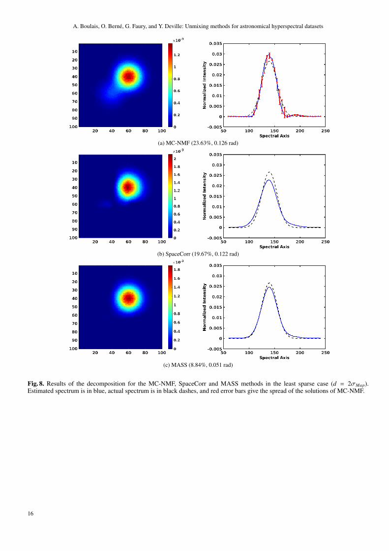
A. Boulais, O. Berne, G. Faury, and Y. Deville: Unmixing methods for astronomical hyperspectral datasets
(a) MC-NMF (23.63%, 0.126 rad)
(b) SpaceCorr (19.67%, 0.122 rad)
(c) MASS (8.84%, 0.051 rad)
Fig. 8. Results of the decomposition for the MC-NMF, SpaceCorr and MASS methods in the least sparse case (d = 2σMap).Estimated spectrum is in blue, actual spectrum is in black dashes, and red error bars give the spread of the solutions of MC-NMF.
16

A. Boulais, O. Berne, G. Faury, and Y. Deville: Unmixing methods for astronomical hyperspectral datasets
(a) SC-NMF-Spec (16.20%, 0.082 rad)
(b) SC-NMF-Map (10.37%, 0.065 rad)
(c) MASS-NMF-Spec (16.69%, 0.080 rad)
(d) MASS-NMF-Map (6.08%, 0.034 rad)
Fig. 9. Results of the decomposition for hybrid methods in the least sparse case (d = 2σMap). Estimated spectrum is in blue, actualspectrum is in black dashes and red error bars give the spread of the solutions.
17

A. Boulais, O. Berne, G. Faury, and Y. Deville: Unmixing methods for astronomical hyperspectral datasets
Appendix A: Data processing methods
A.1. K-means method
K-means is a standard unsupervised classification method (Theodoridis & Koutroumbas (2009)) which aims to partition a set ofN vectors x into k sets σ1, σ2, . . . , σk. Within each set σi, a measure of dissimilarity d between vectors x ∈ σi and clusterrepresentative ci is minimized. The cluster representative ci (or centroid) is the mean vector in the cluster σi. In our case, themeasure of dissimilarity is 1 minus the correlation between x ∈ σi and ci:
d(x, ci) = 1 − corr(x, ci). (A.1)
Performing clustering then amounts to minimizing the following objective function:
J(U,C) =
k∑i=1
N∑j=1
Ui jd(x j, ci), (A.2)
where C is the matrix of centroids ci and U is a partition matrix such that Ui j = 1 if x j ∈ σi and 0 otherwise. Moreover, each vectorbelongs to a single cluster (hard clustering):
k∑i=1
Ui j = 1 j ∈ 1, . . . ,N. (A.3)
The K-means algorithm is defined as follows:
Algorithm 1: K-meansInput : A set of vectors x, the number of cluster k.Output: A partition matrix U, a set of centroids C.
1 begin2 Choose arbitrary initial C0 for the centroids; /* In practice, k vectors x, randomly selected */3 U ← 0;4 repeat
/* Update clusters */5 for j = 1 to N do6 Determine the closest representative, say ci, for x j in the sense of d;7 Ui j ← 1;8 end
/* Update centroids */9 for i = 1 to k do
10 Determine ci as the mean of the vectors x ∈ σi;11 end12 until no change in ci’s occurs between two successive iterations;13 end
However, a well-known drawback of this algorithm is its sensitivity to the initialization, the final centroids depending on thechoice of initial cluster representatives ci. But for our two clustering steps, a manual initialization is possible and avoids thisdrawback:
– As part of Monte-Carlo analysis of NMF (Section 4.1), we use as initial centroids C0 the L spectra estimated by the first Monte-Carlo trial.
– As part of the estimation step of SpaceCorr (Section 4.2), we use as initial centroids C0 the L farthest spectra in the sense of themeasure d (see Eq. (A.1)), among the potential columns of the matrix A.
A.2. Parzen kernel method
The estimation by Parzen kernel or Parzen windows (Theodoridis & Koutroumbas (2009); Silverman (1998)) is a parametric methodfor estimating the probability density function (pdf) of a random variable at any point of its support Ω. Let (x1, x2, . . . , xN) be anindependent and identically distributed sample of a random variable X with an unknown pdf f . Its kernel density estimator is:
f (x) =1
Nh
N∑i=1
K( xi − x
h
)x ∈ Ω, (A.4)
where K is a kernel, i.e., a smooth nonnegative function that integrates to one, and h > 0 is a smoothing parameter called thebandwidth (or width of window). In our case, we use as the kernel the standard normalized Gaussian function (zero expectation andunit standard deviation):
K(x) =1√
2πe(− 1
2 x2). (A.5)
18

A. Boulais, O. Berne, G. Faury, and Y. Deville: Unmixing methods for astronomical hyperspectral datasets
The bandwidth h of the kernel is a free parameter which exhibits a strong influence on the resulting estimate. In the case of aGaussian kernel, it can be shown (Silverman (1998)) that the optimal choice for h is:
h =
(4σ5
3N
) 15
≈ 1.06σN−15 , (A.6)
where σ is the sample standard deviation. The Parzen kernel algorithm is defined as follows:
Algorithm 2: Parzen KernelInput : Sample points X.Output: The estimated pdf f , a support Ω covering the range of the data.
1 begin2 Compute h; /* According to (A.6) */3 Define the support such that Ω = [min(X),max(X)]; /* In practice, Card (Ω) = 100 */4 for k = 1 to Card(Ω) do5 Compute the estimate of f (Ωk); /* According to (A.4) */6 end7 end
Appendix B: Additional test results
The next figures show the performance of the methods applied to all cubes. The SAM and the NRMSE values presented in thefollowing figures are obtained by averaging these measurements for each method over all 100 noise realizations. We also provideerror bars which define the standard deviation over all noise realizations. Each such NMCEB spread measurement is obtained in twostages. Firstly, for each source, the average spectrum and the average envelope are defined over all noise realizations. In a secondstep, we identify the maximum, first along the spectral axis (n) for a given source (`), and then with respect to all sources.
To summarize, we associate with each method a first figure composed of six frames arranged in two rows and three columns.The first row gives the SAM and the second the NRMSE. The first column concerns cubes containing 2 sources, the middle onecontaining 4 sources and the last one containing 6 sources. Within each frame, the x axis gives the distance d defining the overlapbetween the spatial sources, from d = 6σMap down to d = 2σMap. In Sections B.1 to B.7, inside each such frame, the three curvesrespectively correspond to each of the three main noise levels tested in this study: blue for 30 dB Signal to Noise Ratio (SNR), redfor 20 dB and black for 10 dB. Similarly, in Section B.8, inside each frame, the three curves respectively correspond to each of thethree additional tested low SNRs: blue for 5 dB, red for 3 dB and black for 1 dB. For the MC-NMF method and the hybrid methods,we also provide a second figure, consisting of 3 frames giving the NMCEB maximum for each of the 45 cubes.
In conclusion, all of these tests and illustrations aim to quantify several phenomena. First, evaluate the impact of the noiselevel and the distance between the sources on the performance of the methods. Next, quantify the contribution of hybrid methodscompared to the MC-NMF, SpaceCorr and MASS methods used alone. The study of the error bars of the Monte-Carlo analysisassociated with the NMF makes it possible to evaluate the spread of the solutions as a function of the noise level, the sparsity of thesources and the initialization.
B.1. Results with MC-NMF
The performance of the MC-NMF method is shown in Fig. B.1 and B.2. We will first consider the cases involving four or six sources.The performance of MC-NMF then has a low sensitivity to the distance d, i.e. to the source joint sparsity. Similarly, the numberof sources is a criterion having a relatively limited effect on the performance of MC-NMF in our simulations. On the contrary, thenoise level has a significant effect on the quality of the solutions given by MC-NMF (although the noiseless case does not give idealresults). It should be noted that the amplitude of the error bars of MC-NMF depends on all the tested parameters (degree of sparsity,number of sources and noise level). The variability of MC-NMF solutions is often substantial and the goal of hybrid methods is toreduce this variability.
We will now focus on the case of 2 sources. For distances ranging from d = 6σMap down to d = 3σMap (or at least 4σMap),the same comments as those provided above for 4 or 6 sources still apply, as expected. On the contrary, further decreasing d tod = 2σMap results in an unexpected behavior: the SAM and NRMSE values then strongly decrease. In other words, in this situationwhen the sources become more mixed, performance improves. Several causes can lead to this result, such as the presence of noise,the symmetry of the maps, the great similarity of the spectra or the number of iterations of the NMF, although all these featuresalso apply to the cubes containing 4 or 6 sources. To analyze the influence of such features on the shape of the cost function to beminimized and thus on performance, we performed the following additional tests for 2 sources:
– No noise in the mixtures.– Deleting the normalization of the spectra at each iteration of the NMF.– Random switching of columns of X.– Avoiding the symmetry of abundance maps by deforming a 2D Gaussian.– Avoiding the similarity of the spectra by changing the nature of the function simulating the line (triangle or square function).– Fixed number of iterations of the NMF.
19

A. Boulais, O. Berne, G. Faury, and Y. Deville: Unmixing methods for astronomical hyperspectral datasets
– Deleting the observed spectra having a power lower than 90% of the maximal observed power.
Each of these tests led to the same, unexpected, trend as that observed in the first column of Fig B.1. On the contrary, the expectedbehavior was observed in the following additional test, where the sparsity of the sources was varied. The abundance maps simulatedby 2D Gaussians are replaced by a matrix S of dimension 2 × 100 whose elements are drawn with a uniform distribution between0.5 and 1. The first 25 elements of the first row are multiplied by a coefficient α. The elements 26 to 50 of the second row arealso multiplied by the same coefficient α. Thus, depending on the value of α, we simulate more or less sparsity in the data. In thistest, we observe a decrease of the performance of MC-NMF when α increases, i.e. when the source sparsity decreases, as expected.Finally, we performed tests for all the cubes (as well as for the hybrid methods), where we further decreased the distance d tod = 1σMap, which corresponds to very low sparsity. The SAM and NMRSE then considerably increase, which corresponds to theexpected behavior of BSS methods. The above-defined unexpected behavior is therefore only observed in the specific case involving2 sources and the intermediate distance d = 2σMap, and it could be further analyzed in future work.
2 sources 4 sources 6 sources
Fig. B.1. Performances achieved by MC-NMF on the 45 synthetic cubes for 100 realizations of noise with an SNR of 30 dB (inblue), 20 dB (in red), and 10 dB (in black). The error bars give the standard deviation over the 100 realizations of noise.
2 sources 4 sources 6 sources
Fig. B.2. Spread (NMCEB) of the solutions of MC-NMF obtained on the 45 synthetic cubes with 100 realizations of noise.
B.2. Results with SpaceCorr
The performance of the SpaceCorr method is shown in Fig. B.3. This method gives excellent results if the data are sparse enough,i.e., if there are a sufficient number of single-source zones, which here corresponds to a large enough distance d. We also note that
20

A. Boulais, O. Berne, G. Faury, and Y. Deville: Unmixing methods for astronomical hyperspectral datasets
SpaceCorr is not very sensitive to the number of sources. Its (limited) sensitivity is at least due to the fact that the number of sourcesover the considered fixed spatial area may have an influence on the degree of source sparsity in terms of available single-sourcezones. Finally, we emphasize that SpaceCorr is relatively robust to noise in data. The presence of residuals in the estimates ofthe least sparse cases is due to the small number of single-source zones per source in the data. In addition, the step of detectionof the single-source zones is sensitive to the choice of the threshold used to select the best single-source zones. Depending onthis threshold, almost single-source zones may be used to estimate the columns of the mixing matrix, which yields contributionsfrom other sources. However, the sensitivity of the method to the choice of this parameter will be attenuated by hybridization withMC-NMF.
2 sources 4 sources 6 sources
Fig. B.3. Performances achieved by SpaceCorr on the 45 synthetic cubes for 100 realizations of noise with an SNR of 30 dB (inblue), 20 dB (in red), and 10 dB (in black). The error bars give the standard deviation over the 100 realizations of noise.
B.3. Results with SC-NMF-Spec
Whatever the number of sources, the SC-NMF-Spec hybrid version (Fig. B.4) yields results with the same trend as that obtained byMC-NMF used alone for two sources (Fig. B.1, leftmost column). Moreover, when considering two sources for both methods, theyyield similar estimation errors for given sparsity and noise level. Besides, SC-NMF-Spec results in a much lower spread (Fig. B.5)than MC-NMF (Fig. B.2), especially for four or six sources. This property is the main goal of hybridization.
21

A. Boulais, O. Berne, G. Faury, and Y. Deville: Unmixing methods for astronomical hyperspectral datasets
2 sources 4 sources 6 sources
Fig. B.4. Performances achieved by SC-NMF-Spec on the 45 synthetic cubes for 100 realizations of noise with an SNR of 30 dB(in blue), 20 dB (in red), and 10 dB (in black). The error bars give the standard deviation over the 100 realizations of noise.
2 sources 4 sources 6 sources
Fig. B.5. Spread (NMCEB) of the solutions of SC-NMF-Spec obtained on the 45 synthetic cubes with 100 realizations of noise.
B.4. Results with SC-NMF-Map
The SC-NMF-Map hybrid version (Fig. B.6) yields results with the same trend as that obtained by SpaceCorr used alone (Fig.B.3), whatever the number of sources. Moreover, SC-NMF-Map results in significantly lower estimation errors, especially in dif-ficult cases. The spread of the results given by SC-NMF-Map (Fig. B.7) becomes negligible, with an improvement of an order ofmagnitude over the amplitude of the error bars of the SC-NMF-Spec hybrid version.
22

A. Boulais, O. Berne, G. Faury, and Y. Deville: Unmixing methods for astronomical hyperspectral datasets
2 sources 4 sources 6 sources
Fig. B.6. Performances achieved by SC-NMF-Map on the 45 synthetic cubes for 100 realizations of noise with an SNR of 30 dB (inblue), 20 dB (in red), and 10 dB (in black). The error bars give the standard deviation over the 100 realizations of noise.
2 sources 4 sources 6 sources
Fig. B.7. Spread (NMCEB) of the solutions of SC-NMF-Map obtained on the 45 synthetic cubes with 100 realizations of noise.
B.5. Results with MASS
MASS gives excellent results in the case of sufficiently sparse data and in the presence of a reasonable noise level (20 or 30 dBSNR). It is further noted that for mixtures of two or four sources, the results are correct even under the least favorable conditions ofsparsity, again with an SNR of 20 or 30 dB.
The main disadvantage highlighted by the synthetic data tests is the sensitivity of the method to the high level of noise. Indeed,the performances for the mixtures with a 10 dB SNR are weak, even under optimal conditions of sparsity. This sensitivity comesfrom the structure of the method that performs the estimation of the mixing matrix by directly selecting the columns from theobserved vectors. The introduction of a tolerance angle in this selection has an effect at reasonable noise levels but becomes lesseffective at higher noise levels. In addition, reducing the tolerance threshold would allow greater robustness to noise, to the detrimentof component separation. Non single-source observations would then be used in the estimation of the columns of the mixing matrix.The sensitivity of MASS to the noise level can be mitigated by hybridization with MC-NMF.
23

A. Boulais, O. Berne, G. Faury, and Y. Deville: Unmixing methods for astronomical hyperspectral datasets
2 sources 4 sources 6 sources
Fig. B.8. Performances achieved by MASS on the 45 synthetic cubes for 100 realizations of noise with an SNR of 30 dB (in blue),20 dB (in red), and 10 dB (in black). The error bars give the standard deviation over the 100 realizations of noise.
B.6. Results with MASS-NMF-Spec
The MASS-NMF-Spec hybrid version (Fig. B.9) yields the same trends as those obtained by SC-NMF-Spec (Fig. B.4). In com-parison with the MASS method alone, the main advantage is an overall improvement of the performance criteria for mixtures with10 dB SNR. The MASS method used alone in this configuration gave unsatisfactory results. They are markedly improved duringhybridization with MC-NMF. Finally, we note the major decrease in the spread of the solutions given by MASS-NMF-Spec (Fig.B.10) compared to that encountered with the MC-NMF (Fig. B.2), especially for four or six sources. The error bars encounteredhere are of the same order of magnitude as those obtained with SC-NMF-Spec (Fig. B.5).
2 sources 4 sources 6 sources
Fig. B.9. Performances achieved by MASS-NMF-Spec on the 45 synthetic cubes for 100 realizations of noise with an SNR of 30dB (in blue), 20 dB (in red), and 10 dB (in black). The error bars give the standard deviation over the 100 realizations of noise.
24

A. Boulais, O. Berne, G. Faury, and Y. Deville: Unmixing methods for astronomical hyperspectral datasets
2 sources 4 sources 6 sources
Fig. B.10. Spread (NMCEB) of the solutions of MASS-NMF-Spec obtained on the 45 synthetic cubes with 100 realizations of noise.
B.7. Results with MASS-NMF-Map
The MASS-NMF-Map hybrid version (Fig. B.11) yields the same trends as those obtained by MASS used alone (Fig. B.8). Again,there is a noticeable improvement in performance for mixtures with a 10 dB SNR compared to MASS used alone, as well as aclear improvement in the spread of the solutions (Fig. B.12) compared to that obtained with the MC-NMF method alone (Fig. B.2),especially for 4 or 6 sources.
2 sources 4 sources 6 sources
Fig. B.11. Performances achieved by MASS-NMF-Map on the 45 synthetic cubes for 100 realizations of noise with an SNR of 30dB (in blue), 20 dB (in red), and 10 dB (in black). The error bars give the standard deviation over the 100 realizations of noise.
25

A. Boulais, O. Berne, G. Faury, and Y. Deville: Unmixing methods for astronomical hyperspectral datasets
2 sources 4 sources 6 sources
Fig. B.12. Spread (NMCEB) of the solutions of MASS-NMF-Map obtained on the 45 synthetic cubes with 100 realizations of noise.
B.8. Results for very low signal-to-noise ratios
Finally, we performed additional tests for the two methods which appeared to be the most attractive ones in Section 5.3.3, namelyMASS-NMF-Map and SC-NMF-Map. These tests aim at further analyzing the behavior of these preferred methods for very lowSNRs, that is five, three, and one dB. The results thus obtained are shown in Fig. B.13 and B.14. This shows that SC-NMF-Map hereyields significantly better performance than MASS-NMF-Map, as opposed to the results obtained in Section 5.3.3 for significantlyhigher SNRs. This difference is reasonable and coherent with the comments that we provided in Section B.5: although SC-NMF-Map is constraining in terms of sparsity requirements, it has the advantage of averaging the data over an analysis zone (instead ofusing a single point in the basic version of MASS-based methods), which reduces its sensitivity to noise. For very noisy data, such asthose considered here, this feature is of utmost importance, so that SC-NMF-Map yields better performance than MASS-NMF-Map.
2 sources 4 sources 6 sources
Fig. B.13. Performances achieved by SC-NMF-Map on the 45 synthetic cubes for 100 realizations of noise with an SNR of 5 dB (inblue), 3 dB (in red), and 1 dB (in black). The error bars give the standard deviation over the 100 realizations of noise.
26

A. Boulais, O. Berne, G. Faury, and Y. Deville: Unmixing methods for astronomical hyperspectral datasets
2 sources 4 sources 6 sources
Fig. B.14. Performances achieved by MASS-NMF-Map on the 45 synthetic cubes for 100 realizations of noise with an SNR of 5dB (in blue), 3 dB (in red), and 1 dB (in black). The error bars give the standard deviation over the 100 realizations of noise.
27

A. Boulais, O. Berne, G. Faury, and Y. Deville: Unmixing methods for astronomical hyperspectral datasets
B.9. Results for asymmetric scenes
Here we test the effect of breaking the symmetry of the spatial scene presented in Fig 4. We do these by two means, 1) we decreasethe size of some sources, 2) we displace one of the sources outside the square grid considered so far. These two cases are illustratedin Fig. B.15. We have considered other variations as well (e.g. smaller or larger displacement). Overall, the analysis of the resultsshows that the methods provide results with similar performances as for the standard cases described in the core of the paper. Hence,the symmetry of the scene does not appear to be critical, as long as the important hypotheses required by the methods (positivityand sparsity) are verified.
Fig. B.15. Two cases of symmetry breaking for the maps : reduction of the size of two spatial sources (left) and displacement of onesource (right).
28