University of Washington Summer 2014 Department of Economics Eric Zivot Economics 424/CFRM 462 Final Exam Solutions

This is a closed book and closed note exam. However, you are allowed one page of notes (8.5” by 11” or A4 double-sided) and the use of a calculator. Answer all questions and write all answers in the space provided. If you need additional space, you may attach extra sheets of paper with your calculations. Time limit is 2 hours and 10 minutes. Total points = 100.

 

I.ConstantExpectedReturnModel(32points,4pointseach)

 Consider the constant expected return (CER) model

2, ~ (0, )

cov( , ) , ( , )it i it it i

it jt ij it jt ij

r iid N

r r cor r r

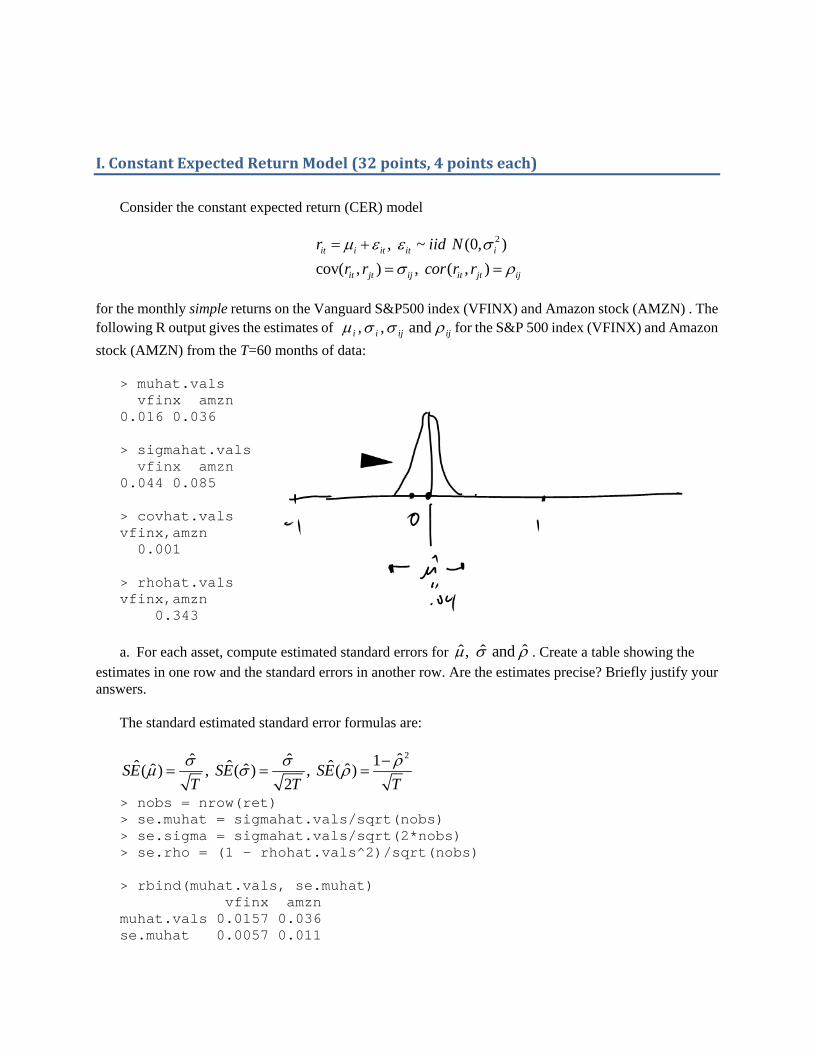
for the monthly simple returns on the Vanguard S&P500 index (VFINX) and Amazon stock (AMZN) . The following R output gives the estimates of ijijii and , , for the S&P 500 index (VFINX) and Amazon

stock (AMZN) from the T=60 months of data: > muhat.vals vfinx amzn 0.016 0.036 > sigmahat.vals vfinx amzn 0.044 0.085 > covhat.vals vfinx,amzn 0.001 > rhohat.vals vfinx,amzn 0.343 a.  For each asset, compute estimated standard errors for ˆˆ ˆ, and . Create a table showing the

estimates in one row and the standard errors in another row. Are the estimates precise? Briefly justify your answers.

The standard estimated standard error formulas are:

2ˆˆ ˆ 1ˆ ˆ ˆ ˆˆ ˆ( ) , ( ) , ( )2

SE SE SET T T

> nobs = nrow(ret) > se.muhat = sigmahat.vals/sqrt(nobs) > se.sigma = sigmahat.vals/sqrt(2*nobs) > se.rho = (1 - rhohat.vals^2)/sqrt(nobs) > rbind(muhat.vals, se.muhat) vfinx amzn muhat.vals 0.0157 0.036 se.muhat 0.0057 0.011

> rbind(sigmahat.vals, se.sigma) vfinx amzn sigmahat.vals 0.04415 0.08489 se.sigma 0.00403 0.00775 > rbind(rhohat.vals, se.rho) vfinx,amzn rhohat.vals 0.343 se.rho 0.114 Standard errors for means are about 1/3 the size of the estimates which indicates that the means are

estimated with moderate imprecision. The standard errors for the volatilities are much smaller than the estimates which indicates precise estimation. The correlation standard error is about 1/3 the size of the estimate and indicates moderate imprecistion.

b. For the S&P 500 index (VFINX) only, compute 95% confidence intervals for , . Briefly

comment on the precision of the estimates. In particular, note if both positive and negative values are in the respective confidence intervals.

The rule‐of‐thumb formula for a 95% confidence interval for a parameter   is   

ˆ ˆ2 ( )SE  

 For VFINX, the estimated standard errors for   and   are 

> # 95% ci for mu > upper = muhat.vals + 2*se.muhat > lower = muhat.vals - 2*se.muhat > cbind(lower[1],upper[1]) [,1] [,2] vfinx 0.00431 0.0271 > # 95% ci for sigma > upper = sigmahat.vals + 2*se.sigma > lower = sigmahat.vals - 2*se.sigma > cbind(lower[1],upper[1]) [,1] [,2] vfinx 0.0361 0.0522 The 95% CI for is fairly wide from an economic point of view (0.5% to 3%), whereas the 95% CI for

is fairly tight from an economic point of view (3.6% to 5.2%). Only positive values are in the confidence intervals.

c. Compute a 95% confidence interval for ,vfinx amzn . Use this interval to test the hypotheses

0 , 1 ,: 0.5 vs. : 0.5vfinx amzn vfinx amznH H using a 5% significance level.

The 95% confidence intervals for  ,vfinx amzn  is 

> upper = rhohat.vals + 2*se.rho > lower = rhohat.vals - 2*se.rho > cbind(lower,upper) lower upper vfinx,amzn 0.116 0.571 Since zero is not in the 95% CI for , we can reject the null hypothesis that = 0 at the 5% level. d. Let W0 = $100,000 be the initial wealth invested in each asset. Estimate the monthly 5%

Value-at-Risk for each asset assuming each asset is normally distributed. Because we have simple returns, the 5% VaR is computed using

.05 .05 0ˆ ˆ ˆ ZVaR q W

> VaR.05 = (muhat.vals + sigmahat.vals*qnorm(0.05))*100000 > VaR.05 vfinx amzn -5692 -10366 e. Briefly explain how you can use the bootstrap to compute a standard error for the monthly 5% normal

VaR for VFINX you computed in part d. above. Bootstrapping involves sampling with replacement from the original data to create B different samples.

On each sample the 5% VaR is computed, and the estimated bootstrap SE is the sample standard deviation of these B 5% VaR values.

f. For VFINX and AMZN Consider testing the hypotheses

0 1: ~ normal vs. : is not normally distributedt tH r H r

using a 5% significance level. The JB statistics are 1.847vfinxJB and 1.512amznJB . What do you

conclude? Under the null of normality, the JB statistic has a chi-square distribution with 2 degrees of freedom.

The 5% critical value is the 95% quantile of the chi-square distribution with 2 degrees of freedom. This quantile is 6. Hence, we reject the null at the 5% significance level if JB > 6. Since both JB values are less than 6, we cannot reject the hypothesis that the returns on both assets are normally distributed.

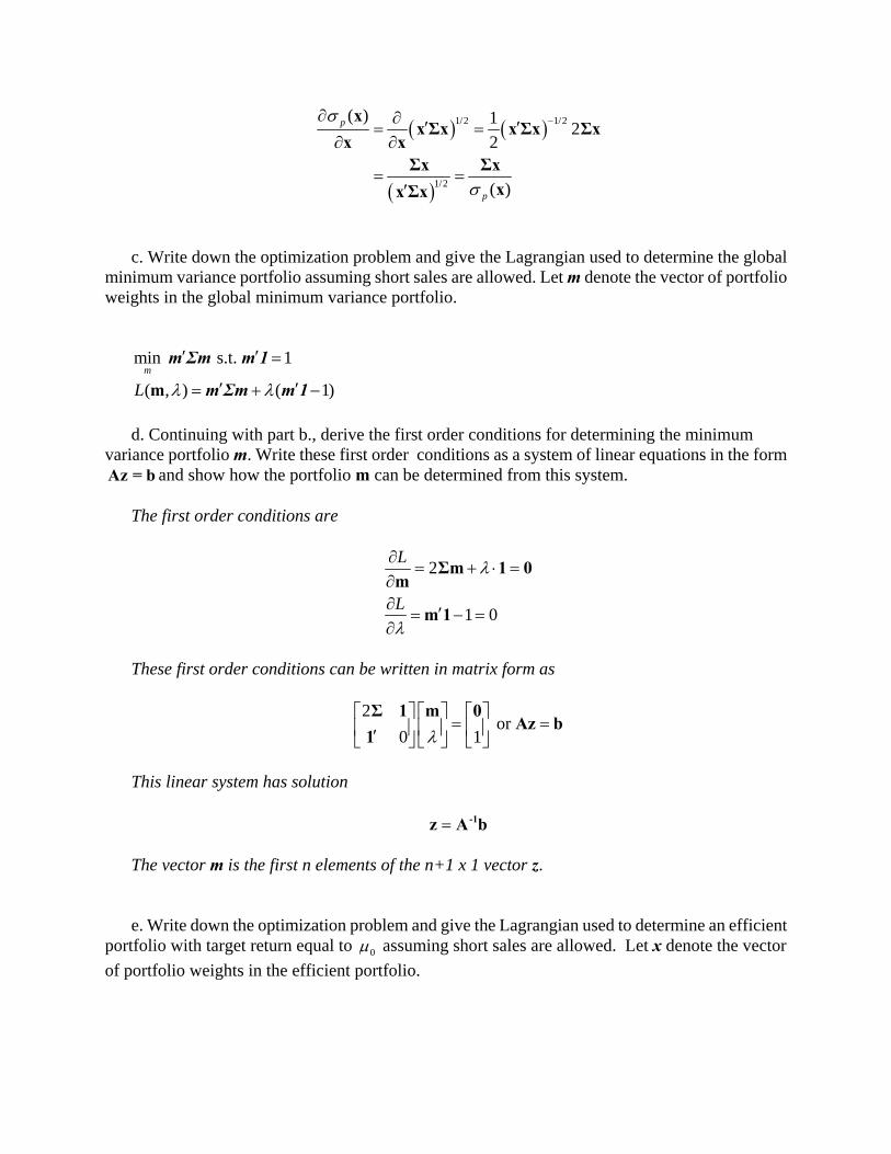
g. The 24-month rolling estimates of and are illustrated in Figure 1 and Figure 2 below (on next

page). The CER model assumes that and are constant over time. Is this a reasonable assumption? Why or why not.

For both VFINX and AMZN, the rolling mean and sd values behave similarly. The means do not move

too much (they both dip a bit in late 2011 and then recover) . The sd values, however, show a slow decline

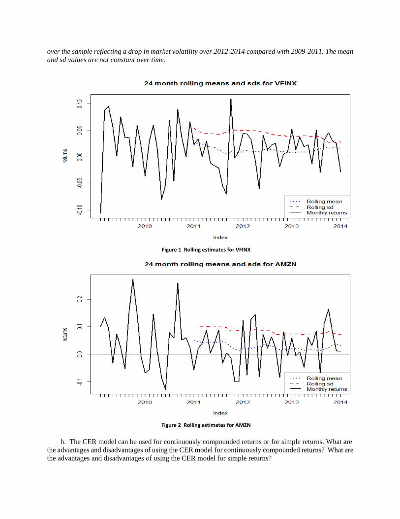
over the sample reflecting a drop in market volatility over 2012-2014 compared with 2009-2011. The mean and sd values are not constant over time.

 Figure 1  Rolling estimates for VFINX 

 Figure 2  Rolling estimates for AMZN 

  h. The CER model can be used for continuously compounded returns or for simple returns. What are

the advantages and disadvantages of using the CER model for continuously compounded returns? What are the advantages and disadvantages of using the CER model for simple returns?

The advantages of the CER model for cc returns: (1) cc returns are more likely normally distributed than simple returns; (2) cc returns are additive over time. The main disadvantage of the CER model for cc returns involves the application to portfolios. The cc return on a portfolio is not a weighted average of the cc returns on the individual assets so the CER model does not hold exactly for portfolios. For simple returns, the main disadvantage is that multiperiod returns are not additive. The CER model does not hold for multiperiod returns. The main advantage, is that the portfolio return is a weighted average of asset returns. Here the CER model holds for portfolios.

II.MatrixAlgebraandPortfolioMath(36points,4pointseach)

Let Ri denote the continuously compounded return on asset i (i = 1, , N) with E[Ri] = i,

var(Ri) = 2i and cov(Ri, Rj) = ij. Define the (N 1) vectors 1, , NR R R , 1( , , )N ,

1, , Nm m m , 1, , Nx x x , 1, , Ny y y , 1, , Nt t t , 1, ,1 1 and the (N N)

covariance matrix

21 12 1

212 2 2

21 2

N

N

N N N

.

The vectors m, x, y and t contain portfolio weights that sum to one. Using simple matrix

algebra, answer the following questions. a. For the portfolios defined by the vectors x and y give the expression for the portfolio returns,

(Rp,x and Rp,y), the portfolio expected returns (p,x and p,y), the portfolio variances ( 2 2, , and p x p y ),

and the covariance between Rp,x and Rp,y ( xy ).

2

, , ,

2, , ,

, ,

, ,

p x p x p x

p y p y p y

xy

R

R

y y

x y

R x x μ x Σx

R y μ Σy

b. For portfolio x, derive the n x 1 vector of marginal contributions to portfolio volatility

defined by

( )p

xMCR

x.

By the chain rule we have

1/2 1/2

1/2

( ) 12

2

( )

p

p

xxΣx xΣx Σx

x xΣx Σx

xxΣx

c. Write down the optimization problem and give the Lagrangian used to determine the global

minimum variance portfolio assuming short sales are allowed. Let m denote the vector of portfolio weights in the global minimum variance portfolio.

min s.t. 1

( , ) ( 1)m

L

m

m Σm m 1

m Σm m 1

d. Continuing with part b., derive the first order conditions for determining the minimum

variance portfolio m. Write these first order conditions as a system of linear equations in the form Az = b and show how the portfolio m can be determined from this system.

The first order conditions are

2

1 0

L

L

Σm 1 0m

m 1

These first order conditions can be written in matrix form as

2 or

0 1

Σ 1 m 0Az b

1

This linear system has solution

-1z A b The vector m is the first n elements of the n+1 x 1 vector z. e. Write down the optimization problem and give the Lagrangian used to determine an efficient

portfolio with target return equal to 0 assuming short sales are allowed. Let x denote the vector

of portfolio weights in the efficient portfolio.

0

1 2 1 2 0

min s.t. 1 and

( , , ) ( 1) ( ) x

L

x

x Σx x 1 x μ

x Σx x 1 x μ

f. Briefly describe how you would compute the efficient frontier containing only risky assets

(Markowitz bullet) when short sales are allowed. Because short sales are allowed, the Markowitz bullet can be constructed using a convex

combination of any two efficient (frontier) portfolio: (1 ) z m x , where m and x are any two frontier portfolios. To get a nice picture, choose portfolio m to be the global minimum variance portfolio and choose the other efficient portfolio x to be the efficient portfolio with target return equal to the highest expected return of the available assets. Then, for example, vary from

1 to -1 in increments of 0.1 and compute z. For each z, compute ,p z z μ and 1/2

,p z z Σz and

then plot these pairs of points. g. Write down the optimization problem used to determine the tangency portfolio, assuming

short sales are not allowed and the risk free rate is given by fr . Let t denote the vector of portfolio

weights in the tangency portfolio.

1/ 2max s.t. 1f

t

r

t -t 1

t Σt

and Niti ,,1 ,0

h. Continuing with part g., is there an analytical solution (i.e., matrix algebra mathematical

formula) for the tangency portfolio when short sales are not allowed? There is no analytical solution for the tangency portfolio when short sales are not allowed. The

inequality constraints do no allow the method of Lagrange multipliers to be used to determine an analytic solution using matrix algebra.

i. Write down the equations for the expected return ( e

p ) and standard deviation ( ep ) of

efficient portfolios consisting of the tangency portfolio and T-bills, where the T-bill rate (risk-free rate) is given by fr and t denotes the vector of portfolio weights in the tangency portfolio.

tan tan tan

2tan tan tan

( ),

,

ep f f

ep

r x r

x

t

t t

 

III.EfficientPortfolios(32points,4pointseach)

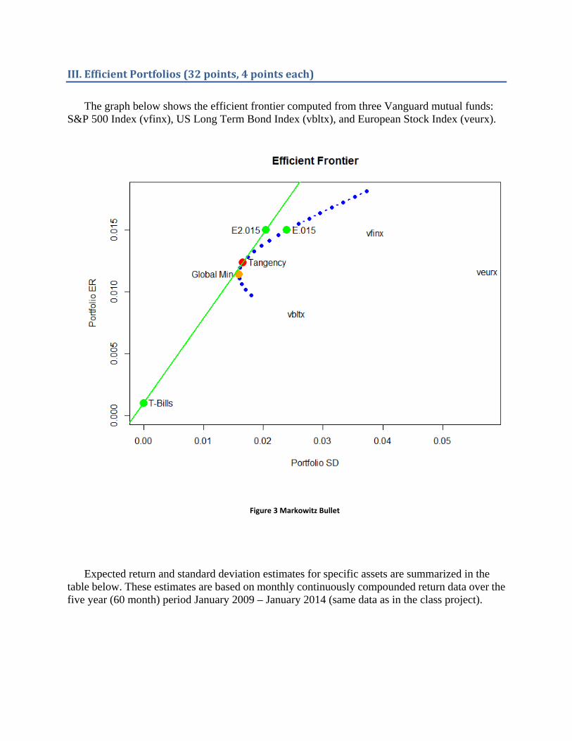
The graph below shows the efficient frontier computed from three Vanguard mutual funds:

S&P 500 Index (vfinx), US Long Term Bond Index (vbltx), and European Stock Index (veurx).

 

Figure 3 Markowitz Bullet Expected return and standard deviation estimates for specific assets are summarized in the

table below. These estimates are based on monthly continuously compounded return data over the five year (60 month) period January 2009 – January 2014 (same data as in the class project).

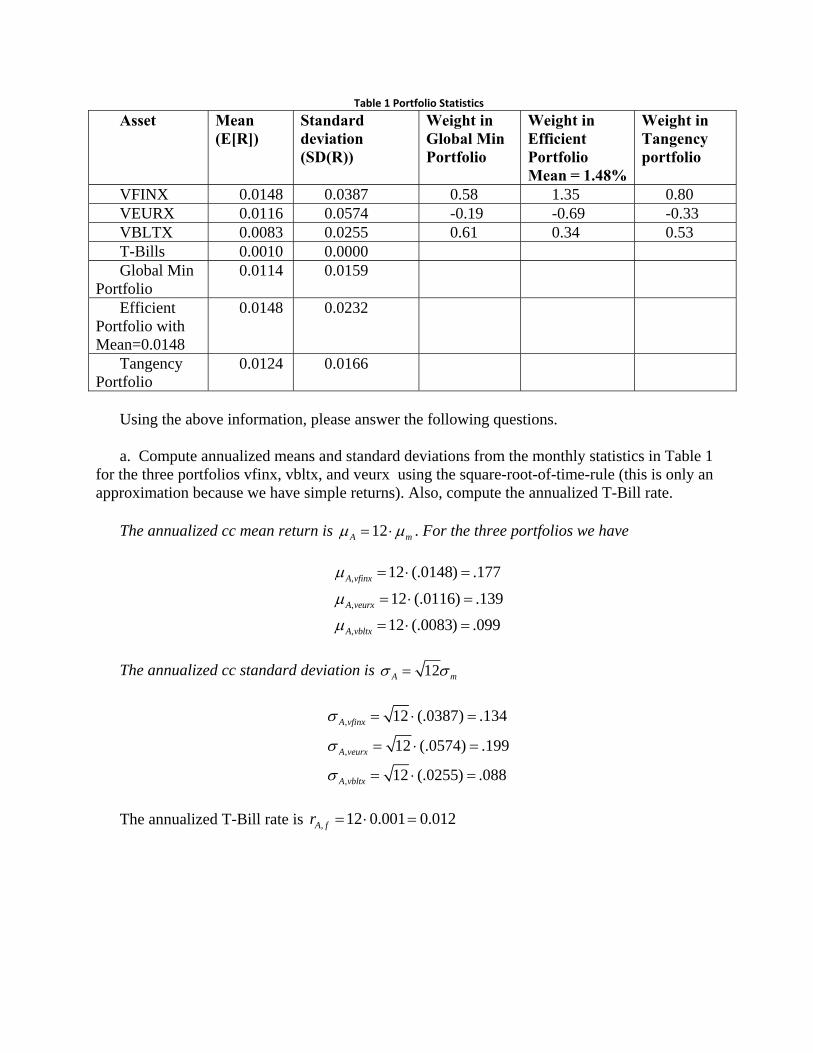
Table 1 Portfolio Statistics 

Asset Mean (E[R])

Standard deviation (SD(R))

Weight in Global Min Portfolio

Weight in Efficient Portfolio Mean = 1.48%

Weight in Tangency portfolio

VFINX 0.0148 0.0387 0.58 1.35 0.80 VEURX 0.0116 0.0574 -0.19 -0.69 -0.33 VBLTX 0.0083 0.0255 0.61 0.34 0.53 T-Bills 0.0010 0.0000 Global Min

Portfolio 0.0114 0.0159

Efficient Portfolio with Mean=0.0148

0.0148 0.0232

Tangency Portfolio

0.0124 0.0166

Using the above information, please answer the following questions. a. Compute annualized means and standard deviations from the monthly statistics in Table 1

for the three portfolios vfinx, vbltx, and veurx using the square-root-of-time-rule (this is only an approximation because we have simple returns). Also, compute the annualized T-Bill rate.

The annualized cc mean return is 12A m . For the three portfolios we have

,

,

,

12 (.0148) .177

12 (.0116) .139

12 (.0083) .099

A vfinx

A veurx

A vbltx

The annualized cc standard deviation is 12A m

,

,

,

12 (.0387) .134

12 (.0574) .199

12 (.0255) .088

A vfinx

A veurx

A vbltx

The annualized T-Bill rate is , 12 0.001 0.012A fr

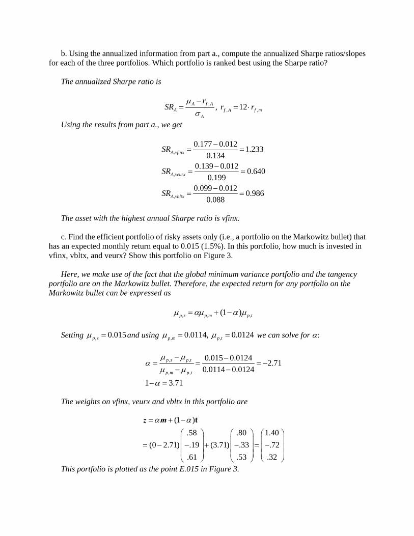
b. Using the annualized information from part a., compute the annualized Sharpe ratios/slopes for each of the three portfolios. Which portfolio is ranked best using the Sharpe ratio?

The annualized Sharpe ratio is

,, ,, 12A f A

A f A f mA

rSR r r

Using the results from part a., we get

,

,

,

0.177 0.0121.233

0.1340.139 0.012

0.6400.199

0.099 0.0120.986

0.088

A vfinx

A veurx

A vbltx

SR

SR

SR

The asset with the highest annual Sharpe ratio is vfinx. c. Find the efficient portfolio of risky assets only (i.e., a portfolio on the Markowitz bullet) that

has an expected monthly return equal to 0.015 (1.5%). In this portfolio, how much is invested in vfinx, vbltx, and veurx? Show this portfolio on Figure 3.

Here, we make use of the fact that the global minimum variance portfolio and the tangency

portfolio are on the Markowitz bullet. Therefore, the expected return for any portfolio on the Markowitz bullet can be expressed as

, , ,(1 )p z p m p t

Setting , 0.015p z and using , ,0.0114, 0.0124p m p t we can solve for :

, ,

, ,

0.015 0.01242.71

0.0114 0.0124

1 3.71

p z p t

p m p t

The weights on vfinx, veurx and vbltx in this portfolio are

(1 )

.58 .80 1.40

(0 2.71) .19 (3.71) .33 .72

.61 .53 .32

tz m

This portfolio is plotted as the point E.015 in Figure 3.

We can get the same answer if we use the global minimum variance portfolio and the efficient portfolio with expected return equal to 1.48%. The calculations are essentially the same:

, , ,(1 )p z p m p e

Setting , 0.015p z and using , ,0.0114, 0.0148p m p e we can solve for :

, ,

, ,

0.015 0.01480.06

0.0114 0.0148

1 1.06

p z p e

p m p e

The weights on vfinx, veurx and vbltx in this portfolio are

(1 )

.58 1.35 1.40

( 0.06) .19 (1.06) .69 .72

.61 .34 0.32

z m x

d. How much should be invested in T-bills and the tangency portfolio to create an efficient portfolio with expected return equal to 0.015 (1.5%) ? What is the standard deviation of this efficient portfolio? Indicate the location of this efficient portfolio on Figure 3.

tantan

tan

, tan tan

.015 .01 0.0011.23

.0124 0.001

1 1 1.23 0.23

(1.23)(0.0166) 0.024

f

f

f

p e

rx

r

x x

x

This portfolio is plotted as the point E2.015 in Figure 3. e. In the efficient portfolio you found in part d, what are the shares of wealth invested in

T-Bills, vfinx, vbltx, and veurx? vfinx veurx vbltx T-Bills 1.23*(0.80)=0.99 1.23*(-0.33)=-0.41 1.23*(0.53)=0.65 -0.23 f. Assuming an initial $100,000 investment for one month, compute the 5% value-at-risk based

on the normal distribution for the global minimum variance portfolio. First we find the 5% quantiles for the global minimum variance portfolio

.05: 0.0114 (0.0159)( 1.645) 0.0147port q

Then we compute the 5% VaR

.05: $100,000 ( 0.0147) $1,473port VaR

> w0 = 100000 > q.05 = gmin.port$er + gmin.port$sd*qnorm(0.05) > q.05 [1] -0.0147 > VaR.05 = q.05*w0 > VaR.05 [1] -1473 g. The efficient frontier of risky assets shown in Figure 3 allows for short sales (see the weights

in the portfolios listed in Table 1). Using the space below, copy the efficient frontier from Figure 3 and indicate roughly the location of the efficient frontier of risky assets that does not allow short sales.

h. Suppose you want to find the efficient portfolio of risky assets only that has an expected

monthly return equal to 0.02 (2%) but that you are prevented from short selling. Is it possible to find such an efficient portfolio? Briefly explain why or why not.

It is not possible to find an efficient portfolio of risky assets only that has an expected return of

2%. To see this, from Table 1 above notice that the efficient portfolio with expected return equal to 1.48% has a short position in veurx and the tangency portfolio (with mean 1.24%) has a short position in veurx as well. Hence, for an efficient portfolio with mean 2% we would need a short position in veurx.