Download (757Kb) - USQ ePrints - University of Southern Queensland
University of Southern Queensland
Faculty of Engineering and Surveying
Comparison of PV maximum power point.
A dissertation submitted by
Mr Christopher KIRBY
In fulfilment of the requirements of
Bachelor of Engineering (Electrical and Electronic)
October, 2015.

i
Abstract
Photovoltaic technology began in 1876 with the development of the selenium solar cell,
although the limited electrical energy generated was not enough to power any useful
machine. Experimentation during the 1950’s with alternate materials led to the
development of the first silicon based cell. The new silicon cell was selected for use in
space exploration to provide a longer lasting energy supply. Modern solar panels are
commonly used across the country as part of a distributed electricity supply network.
The electrical power generated by a photovoltaic solar panel will be affected by a large
number of factors, ranging from light irradiance level, light angle, location, electrical load
on the panels and the configuration of the connection with adjacent panels.
Simulations conducted within Matlab were used to assess the effect of various energy
reduction factors when a multiple direction oriented panels are connected in common.
The series connected system provided the best level of immunity for the case having
unequal levels of shading. The parallel configuration performed better for each of the
other cases tested, including mismatched voltage and current specifications, irradiance
level, ambient temperature and only angular offset.
The efficiency of a solar panel decreases with increased cell temperature. Natural
convection currents surrounding the panel assist with cooling and are increase with a
larger panel tilt angle. Experimentation results indicated a linear increase in the panel
efficiency of approximately 0.05% per degree tilt increase.
The optimum azimuth and tilt angles vary depending on the installation location. Data
obtained using the Homer microgrid modelling package was used to identify the optimum
installation angles for four locations throughout Australia. A mathematical model was
developed to describe the azimuth and tilt relationship. Further modelling conducted
using Homer included a second photovoltaic string. Simulations of different inverter
configurations indicated the dual power point tracking provided the best efficiency for all
situations. Single power point tracking and separate inverters were able to demonstrate
similar efficiencies when components of the installation were matched, and panels were
installed on a common orientation.

ii
The goal of this project was to provide information which could assist designers of solar
generation installations maximise the electrical energy generated over the life of the
system.
The recommendations are the correct inverter selection, prioritisation of the most north
facing roof surface, and setting tilt angle relative to the actual installation azimuth will
deliver superior energy yields than a generalised installation approach.

iii
University of Southern Queensland
Faculty of Health, Engineering and Sciences
ENG4111/ENG4112 Research Project
Limitations of Use
The Council of the University of Southern Queensland, its Faculty of Health, Engineering
& Sciences, and the staff of the University of Southern Queensland, do not accept any
responsibility for the truth, accuracy or completeness of material contained within or
associated with this dissertation.
Persons using all or any part of this material do so at their own risk, and not at the risk of
the Council of the University of Southern Queensland, its Faculty of Health, Engineering
& Sciences or the staff of the University of Southern Queensland.
This dissertation reports an educational exercise and has no purpose or validity beyond
this exercise. The sole purpose of the course pair entitled “Research Project” is to
contribute to the overall education within the student’s chosen degree program. This
document, the associated hardware, software, drawings, and other material set out in the
associated appendices should not be used for any other purpose: if they are so used, it is
entirely at the risk of the user.

iv
Certification of work
I certify the information and work contained within this dissertation, including computer
assisted modelling, experimentation, calculated results, analysis and conclusions are
entirely my own work, excepting where indication of another source and
acknowledgement has been provided.
I further certify this work is original and has not been previously been submitted in any
other course or institution.
Christopher Kirby
0050093295

v
Acknowledgements
This research was conducted under the supervision of Catherine Hills, providing advice
and assistance during the course of this dissertation.
I would also like to acknowledge the assistance of the following people,
Gemma for patience and support throughout the course of my study.
Madison for patience throughout this dissertation.
John and Carol Kirby for assistance looking after Madison.
Andreas Helwig for providing the main project idea and assisting in the development
of ideas.
Les Bowtell for advice regarding convective cooling of panels and assistance to
conduct thermal cooling experimentation.
Wayne Cheary for listening to the endless volumes of information I have reviewed
and also for providing advice on avenues of research.
Antony Zizimou for listening to the information I have reviewed.
Homer Energy for the use of their microgrid modelling software.
vi
Table of Contents
Abstract .............................................................................................................................. i
Limitations of Use ............................................................................................................ iii
Certification of work ........................................................................................................ iv
Acknowledgements ........................................................................................................... v
Table of Contents ............................................................................................................. vi
List of figures .................................................................................................................. xii
List of tables ................................................................................................................... xvi
1. Introduction ........................................................................................................... 1
2. Literature review. .................................................................................................. 2
History of photovoltaic technology. .................................................... 2
Construction of photovoltaic systems. ................................................. 3
2.2.1. Cell construction. ................................................................................. 3
2.2.2. Panel construction. ............................................................................... 4
2.2.3. Series or parallel connected cells. ........................................................ 4
2.2.4. Inverters. .............................................................................................. 5
Principle of photovoltaic operation...................................................... 5
2.3.1. PV cell power output. .......................................................................... 6
Incident solar energy. ......................................................................... 7
Cell size. ............................................................................................ 8
Light angle. ........................................................................................ 8
Light reflection. ............................................................................... 10
Panel loading ................................................................................... 11
Panel / Cell design and manufacturing ............................................. 11
Panel shading. .................................................................................. 13
Panel efficiency ............................................................................... 13
Panel age........................................................................................... 14

vii
Temperature...................................................................................... 14
Installation design ............................................................................ 16
Air mass ............................................................................................ 16
Inverter design ................................................................................... 17
2.4.1. Introduction to converters. ................................................................. 17
2.4.2. Operation of inverters. ....................................................................... 17
2.4.3. Grid fed inverters. .............................................................................. 18
2.4.4. Single stage inverters. ........................................................................ 18
2.4.5. Multiple stage inverters. .................................................................... 18
2.4.6. Inverter efficiency. ............................................................................. 19
Over voltage ..................................................................................... 19
Under voltage .................................................................................. 19
Over power ...................................................................................... 19
Under power .................................................................................... 20
2.4.7. Maximum power point tracking. ....................................................... 20
Perturb and observe. ........................................................................ 20
Incremental conductance. ................................................................ 21
Modelling ........................................................................................... 22
2.5.1. IV Curve Modelling ........................................................................... 22
IV and PV curves. ............................................................................ 23
Location of maximum power point. ................................................ 24
3. Project planning. ................................................................................................. 25
Ethics. ................................................................................................ 25
Methodology. ..................................................................................... 25
3.2.1. Required resources. ............................................................................ 25
3.2.2. Identification and sourcing of relevant literature. .............................. 26
3.2.3. Modelling multiple interconnected solar panels. ............................... 26

viii
3.2.4. Modelling solar panel optimum angle. .............................................. 27
3.2.5. Modelling multiple string systems. .................................................... 28
3.2.6. Selection of installation locations. ..................................................... 28
Brooklyn Park, S.A. ......................................................................... 29
Toowoomba, Qld. ............................................................................ 30
.Darwin, N.T. ................................................................................... 31
Hobart, Tas. ..................................................................................... 32
3.2.7. Panel angle effect on cooling. ............................................................ 33
3.2.8. Development of installation guidelines. ............................................ 33
Project timeline. ................................................................................. 34
Assessment of consequential effects.................................................. 35
3.4.1. Identification of hazards. ................................................................... 36
3.4.2. Risk assessment. ................................................................................ 36
3.4.3. Risk matrix scores. ............................................................................. 37
3.4.4. Risk assessment outcomes. ................................................................ 37
3.4.5. Project hazard identification and risk assessment.............................. 38
4. Results ................................................................................................................. 39
IV Curve modelling. .......................................................................... 39
4.1.1. Differing panel angle. ........................................................................ 40
4.1.2. Hard shading panels with varied panel angle. ................................... 42
Equal shaded area. ........................................................................... 42
Unequal shaded area: Parallel connected. ....................................... 44
Unequal shaded area: Series connected. .......................................... 47
4.1.3. Mismatched panel specifications. ...................................................... 50
Mismatched voltage specifications: Parallel connection ................. 50
Mismatched voltage specifications: Series connection ................... 52
Mismatched current specifications: Parallel connection. ................ 53
ix
Mismatched current specifications: Series connection. ................... 55
4.1.4. Varied temperature. ........................................................................... 56
Varied temperature: Parallel connection ......................................... 57
Varied temperature: Series connection ............................................ 59
4.1.5. Varied irradiance................................................................................ 61
Varied irradiance: Parallel connection ............................................. 61
Varied irradiance: Series connection ............................................... 63
Thermal cooling experimentation. ..................................................... 65
Homer energy modelling. .................................................................. 67
4.3.1. Single string ....................................................................................... 67
Optimum installation angle: 15 degree resolution. .......................... 68
Optimum installation angle: 1 degree resolution. ............................ 69
Site position effect on optimum installation angle. ......................... 71
Site position effect on optimum tilt without optimum azimuth. ..... 73
Model for determination of optimum tilt and azimuth. ................... 73
Single panel model using calculated tilt installation angles. ............ 76
4.3.2. Dual string modelling. ....................................................................... 78
5. Conclusion .......................................................................................................... 79
Further work. ..................................................................................... 80
6. References ........................................................................................................... 81
Project Specification ..............................................................................
Project timeline ......................................................................................
Derivation of formulas ...........................................................................
Current voltage relationship: IV curve ............................................. C1
Solar panel model ............................................................................. C1
Solar panel model error..................................................................... C2
Optimum azimuth ............................................................................. C8

x
Optimum tilt .................................................................................... C12
Optimum tilt correction factor ( C ) ................................................ C16
Matlab code............................................................................................
Function: Solar_Panel_Model_Par ................................................... D1
Function: Solar_Panel_Model_Ser ................................................... D2
Script: Efficiency_calculator_Par ..................................................... D4
Script: Efficiency_calculator_Ser ..................................................... D9
Script: Error Search ........................................................................ D14
Script: Varied_Irradiance_Plot ....................................................... D15
Script: Varied_Temperature_Plot ................................................... D16
Modelling results ...................................................................................
Optimum installation plots ............................................................... E1
Brooklyn Park. .................................................................................. E1
Toowoomba ...................................................................................... E3
Darwin. ............................................................................................. E5
Hobart. .............................................................................................. E7
Location offset plots ......................................................................... E9
Brooklyn Park. .................................................................................. E9
Toowoomba .................................................................................... E11
Darwin. ........................................................................................... E13
Hobart. ............................................................................................ E15
Hazard identification and risk assessments ...........................................
Hazard identification.......................................................................... F1
Solar installations ............................................................................... F1
Project. ............................................................................................... F2
Risk matrix scores. ............................................................................. F2
Risk assessment. ................................................................................ F3

xi
Solar installations ............................................................................... F3
Project. ............................................................................................... F5
Specification sheets
Hareon Solar specification sheet ....................................................... G1
Tindo Solar specification sheet ......................................................... G3
xii
List of figures
Figure 2.1 – Photovoltaic cell cross section ...................................................................... 3
Figure 2.2 – Cell, Module, Panel and array relationship .................................................. 4
Figure 2.3 – Photovoltaic operation .................................................................................. 6
Figure 2.4 – Solar radiation and electromagnetic spectrum .............................................. 7
Figure 2.5 – Light reflection characteristics ................................................................... 10
Figure 2.6 – Generalised IV curve power voltage curve ................................................ 11
Figure 2.7 – Generalised IV curve power voltage curve, varied temperature ................ 14
Figure 2.8 – Perturb and observe flowchart .................................................................... 21
Figure 2.9 – Incremental conductance flowchart ............................................................ 22
Figure 3.1 – Brooklyn Park site overview ...................................................................... 29
Figure 3.2 – Toowoomba site overview .......................................................................... 30
Figure 3.3 – Darwin site overview .................................................................................. 31
Figure 3.4 – Hobart site overview ................................................................................... 32
Figure 4.1a –Parallel MPPT: Panel 1: 0°, Panel 2: 0°-56°. ............................................. 40
Figure 4.1b –Series MPPT: Panel 1: 0°, Panel 2: 0°-56°. ............................................... 41
Figure 4.2a –Parallel MPPT: 1/3 panel shading.............................................................. 43
Figure 4.2b –Series MPPT: 1/3 panel shading. ............................................................... 43
Figure 4.3a –Parallel MPPT: Panel 1 @ 2/3 & Panel 2 @ unshaded. ............................ 44
Figure 4.3b – Parallel MPPT: Panel 1 @ 2/3 & Panel 2 @ 1/3 shading. ........................ 45
Figure 4.4a – Parallel MPPT: Panel 1 unshaded & Panel 2 @ 2/3 shading. .................. 46
Figure 4.4b – Parallel MPPT: Panel 1 @ 1/3 & Panel 2 @ 2/3 shading. ........................ 46
Figure 4.5a – Series MPPT: Panel 1 @ unshaded & Panel 2 @ 1/3 shading. ................ 47
Figure 4.5b – Series MPPT: Panel 1 @ unshaded & Panel 2 @ 2/3 shading. ................ 48
Figure 4.6a – Series MPPT: Panel 1 @ 2/3 shaded & Panel 2 @ unshaded. .................. 49
Figure 4.6b – Series MPPT: Panel 1 @ 2/3 shaded & Panel 2 @ 1/3 shading. .............. 49
xiii
Figure 4.7a –Parallel MPPT: Voc @ 29.0V & 30.8V..................................................... 51
Figure 4.7b – Parallel MPPT: Voc @ 30.8V & 29.0V ................................................... 51
Figure 4.8b –Series MPPT: Voc @ 30.8V & 29.0V ....................................................... 53
Figure 4.9a –Parallel MPPT: ISC @ 8.11A & 8.61A ....................................................... 54
Figure 4.9b – Parallel MPPT: ISC @ 8.61A & 8.11A ..................................................... 54
Figure 4.10a –Series MPPT: ISC @ 8.11A & 8.61A ....................................................... 55
Figure 4.10b – Series MPPT: ISC @ 8.61A & 8.11A ...................................................... 56
Figure 4.11a – Parallel MPPT: T @ 25°C ...................................................................... 57
Figure 4.11b – Parallel MPPT: T @ 15°C ...................................................................... 58
Figure 4.11c – Parallel MPPT: T @ 35°C ...................................................................... 58
Figure 4.12a – Series MPPT: T @ 25°C ......................................................................... 59
Figure 4.12b – Series MPPT: T @ 15°C ......................................................................... 60
Figure 4.12c – Series MPPT: T @ 35°C ......................................................................... 60
Figure 4.13a – Parallel MPPT: G @ 1000W/m² ............................................................. 62
Figure 4.13b – Parallel MPPT: G @ 800W/m² ............................................................... 62
Figure 4.13c – Parallel MPPT: G @ 400W/m² ............................................................... 63
Figure 4.14a – Series MPPT: G @ 1000W/m² ............................................................... 64
Figure 4.14b – Series MPPT: G @ 800W/m² ................................................................. 64
Figure 4.14c – Series MPPT: G @ 400W/m² ................................................................. 65
Figure 4.15 – Normalised cell temperature ..................................................................... 66
Figure 4.16 – Tilt angle efficiency .................................................................................. 67
Figure 4.17a – Brooklyn Park optimum tilt angle and generated power. ....................... 69
Figure 4.17b – Brooklyn Park optimum tilt angle and generated power. ....................... 70
Figure 4.18 – Optimum tilt angle change per° of latitude versus panel azimuth. ........... 73
Figure 4.19 – Optimum azimuth calculated model error. ............................................... 75
Figure 4.20 – Optimum tilt calculated model error......................................................... 76

xiv
Figure 4.21 – Generated power: 2 string 3kW at Azimuth 177. ..................................... 78
Figure C.1a – Varied irradiance model. ......................................................................... C3
Figure C.1b – Bellini et al. Varied irradiance. ............................................................... C4
Figure C.2a – Varied temperature model. ...................................................................... C4
Figure C.2b – Bellini et al. Varied temperature. ............................................................ C5
Figure C.3a – Model VOCM vs irradiance. ...................................................................... C6
Figure C.3b – Corrected VOCM vs irradiance ................................................................. C6
Figure C.4a – Varied irradiance corrected. .................................................................... C7
Figure C.4b – Varied temperature corrected. ................................................................. C7
Figure E.1 – Brooklyn Park optimum tilt angle & generated power: 15° resolution .... E1
Figure E.2 – Brooklyn Park generated power surface plot: 15° resolution ................... E2
Figure E.3 – Brooklyn Park optimum tilt angle and generated power: 1° resolution .... E2
Figure E.4 – Brooklyn Park generated power surface plot: 2° resolution ..................... E2
Figure E.5 – Toowoomba optimum tilt angle and generated power: 15° resolution ..... E3
Figure E.6 – Toowoomba generated power surface plot: 15° resolution ....................... E3
Figure E.7 – Toowoomba optimum tilt angle and generated power: 1° resolution ....... E4
Figure E.8 – Toowoomba generated power surface plot: 2° resolution ......................... E4
Figure E.9 – Darwin optimum tilt angle and generated power: 15° resolution ............. E5
Figure E.10 – Darwin generated power surface plot: 15° resolution ............................. E5
Figure E.11 – Darwin optimum tilt angle and generated power: 1° resolution ............. E6
Figure E.12 – Darwin generated power surface plot: 2° resolution ............................... E6
Figure E.13 – Hobart optimum tilt angle and generated power: 15° resolution ............ E7
Figure E.14 – Hobart generated power surface plot: 15° resolution .............................. E7
Figure E.15 – Hobart optimum tilt angle and generated power: 1° resolution .............. E8
Figure E.16 – Hobart generated power surface plot: 2° resolution ................................ E8
Figure E.17 – Brooklyn Park 5°N generated power surface plot: 2° resolution ............ E9
xv
Figure E.18 – Brooklyn Park 5°S generated power surface plot: 2° resolution ............. E9
Figure E.19 – Brooklyn Park 5°E generated power surface plot: 2° resolution .......... E10
Figure E.20 – Brooklyn Park 5°W generated power surface plot: 2° resolution ......... E10
Figure E.21 – Toowoomba 5°N generated power surface plot: 2° resolution ............. E11
Figure E.22 – Toowoomba 5°S generated power surface plot: 2° resolution .............. E11
Figure E.23 – Toowoomba 5°E generated power surface plot: 2° resolution .............. E12
Figure E.24 – Toowoomba 5°W generated power surface plot: 2° resolution ............ E12
Figure E.25 – Darwin 5°N generated power surface plot: 2° resolution ..................... E13
Figure E.26– Darwin 5°S generated power surface plot: 2° resolution ....................... E13
Figure E.27 – Darwin 5°E generated power surface plot: 2° resolution ...................... E14
Figure E.28 – Darwin 5°W generated power surface plot: 2° resolution .................... E14
Figure E.29 – Hobart 5°N generated power surface plot: 2° resolution ...................... E15
Figure E.30 – Hobart 5°S generated power surface plot: 2° resolution ....................... E15
Figure E.32 – Hobart 5°W generated power surface plot: 2° resolution ..................... E16
Figure G.1a – Hareon solar specification sheet ............................................................. G1
Figure G.1b – Hareon solar specification sheet ............................................................. G2
Figure G.2a – Tindo solar specification sheet ..................................................................... G3
Figure G.2b – Tindo solar specification sheet .................................................................. G4
xvi
List of tables
Table 4.1 – Optimum installation angles and generated power. ..................................... 70
Table 4.2 – Optimum installation at varied site location. ............................................... 72
Table 4.3 – Calculated optimum installation angles. ...................................................... 77
Table B.1 – Project timeline........................................................................................... B1
Table C.1 – IV curve input parameters. ......................................................................... C3
Table C.2 – Non optimum tilt angle scaling relative to optimum tilt. ......................... C16
Table F.1 – Risk management score. .............................................................................. F3
Table F.2 – Risk score. .................................................................................................... F3
Table F.3 – Risk assessment: Solar installation. ............................................................. F4
Table F.4 – Risk assessment: Project. ............................................................................. F5

1
1. Introduction
Solar panels are widely used throughout our community for the generation of electrical
power. The aim of this project will be to determine the installation parameters for solar
panel installations which maximises the energy generated throughout the life of the
installation, and reducing carbon emissions from electrical power generation. Matlab will
be used to model the effect of various environmental factors, installation parameters and
connection configurations on the output of a small scale solar system. Homer microgrid
software will be used to determine the parameters for optimum installation, and the effect
of various configurations to the annual power generation. The final section will include
guidelines for installation to achieve maximum power generation.
2
2. Literature review.
The main focus of this project is to optimise the operating efficiency of solar energy
systems throughout Australia. There is a large amount of literature available relating to
factors which affect the efficiency photovoltaic cells. Standardised test parameters have
been adopted by the industry for the testing of solar panels. (National Instruments, 2009a)
A majority of the information relating to solar panel efficiency has been sourced from
works where the author or sponsoring organisation is involved in research of photovoltaic
technology.
History of photovoltaic technology.
The discovery of the photoelectric effect was the result of experiments conducted by
William Grylls Adams and Richard Evans Day in 1876. The experimentation involved
subjecting selenium to a light source and observing the resulting electrical current
produced. The power generated by solar cells manufactured using selenium was
insufficient to power any equipment. (Perlin, n.d)
In 1953, scientists at Bell Laboratories produced a silicon based solar cell while
researching possible uses of silicon within the electronic industry. The resulting cell
generated significantly more power than the selenium cell. The demand for silicon solar
cells for power generation applications was limited due to the high cost of manufacturing
the cells. (Perlin, n.d)
With the development of earth orbiting satellites and the associated electronic systems,
an energy supply lasting longer than conventional batteries was required. Silicon based
solar cells provided the solution, leading to a demand for the technology. (Perlin, n.d)
Throughout the 1970’s continued development into silicon based solar technology led to
a deduction of the per watt unit cost. The cost limited demand for use in remote locations,
not serviced through mains power grids. (Perlin, n.d)
3
Recent years has seen the technology expanded to small scale distributed electricity
generation. Each month, over 15000 systems are installed throughout Australia. The total
installed capacity exceeded 4GW prior to the end of 2014. (Renew Economy, 2015)
Construction of photovoltaic systems.
2.2.1. Cell construction.
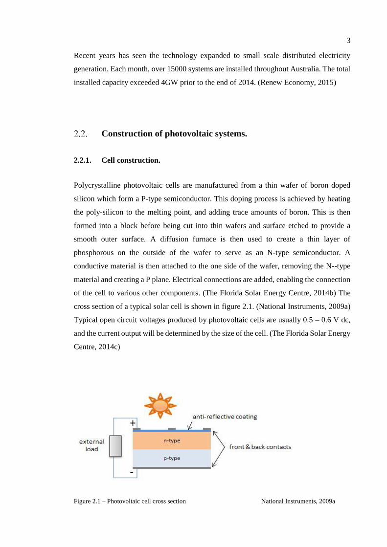
Polycrystalline photovoltaic cells are manufactured from a thin wafer of boron doped
silicon which form a P-type semiconductor. This doping process is achieved by heating
the poly-silicon to the melting point, and adding trace amounts of boron. This is then
formed into a block before being cut into thin wafers and surface etched to provide a
smooth outer surface. A diffusion furnace is then used to create a thin layer of
phosphorous on the outside of the wafer to serve as an N-type semiconductor. A
conductive material is then attached to the one side of the wafer, removing the N--type
material and creating a P plane. Electrical connections are added, enabling the connection
of the cell to various other components. (The Florida Solar Energy Centre, 2014b) The
cross section of a typical solar cell is shown in figure 2.1. (National Instruments, 2009a)
Typical open circuit voltages produced by photovoltaic cells are usually 0.5 – 0.6 V dc,
and the current output will be determined by the size of the cell. (The Florida Solar Energy
Centre, 2014c)
Figure 2.1 – Photovoltaic cell cross section National Instruments, 2009a
4
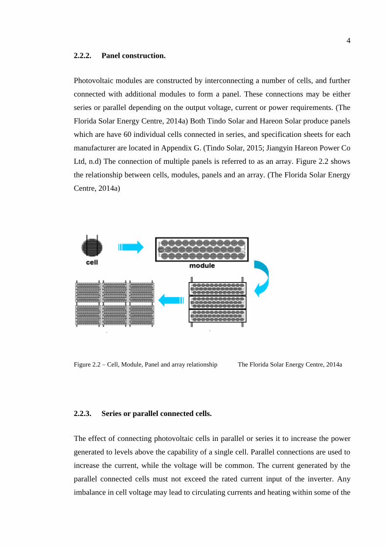
2.2.2. Panel construction.
Photovoltaic modules are constructed by interconnecting a number of cells, and further
connected with additional modules to form a panel. These connections may be either
series or parallel depending on the output voltage, current or power requirements. (The
Florida Solar Energy Centre, 2014a) Both Tindo Solar and Hareon Solar produce panels
which are have 60 individual cells connected in series, and specification sheets for each
manufacturer are located in Appendix G. (Tindo Solar, 2015; Jiangyin Hareon Power Co
Ltd, n.d) The connection of multiple panels is referred to as an array. Figure 2.2 shows
the relationship between cells, modules, panels and an array. (The Florida Solar Energy
Centre, 2014a)
Figure 2.2 – Cell, Module, Panel and array relationship The Florida Solar Energy Centre, 2014a
2.2.3. Series or parallel connected cells.
The effect of connecting photovoltaic cells in parallel or series it to increase the power
generated to levels above the capability of a single cell. Parallel connections are used to
increase the current, while the voltage will be common. The current generated by the
parallel connected cells must not exceed the rated current input of the inverter. Any
imbalance in cell voltage may lead to circulating currents and heating within some of the
5
cells. (MPPT Solar, n.d a) Cells which are connected in series increase the current, while
maintaining a common voltage throughout the series link. The series connected string
must be configured so the maximum voltage output does not exceed the specified voltage
rating of the inverter. (MPPT Solar, n.d.b)
2.2.4. Inverters.
Inverters are electronic devices which are used to convert DC power into AC for use
throughout the home, or exporting to the mains electricity grid. (Ahfock, 2011) Maximum
power point tracking is a feature associated with modern solar inverters. This maximises
the power generated by a photovoltaic panel. (National Instruments, 2009c)
Principle of photovoltaic operation
The photovoltaic effect is the principle of converting energy stored within light photons
into electrical energy is shown in figure 2.3 (The Florida Solar Energy Centre, 2014c),
using silicon based semiconductor materials. Photons within the spectrum of energy
emitted by the sun, and colliding with a photovoltaic cell cause an energy increase of the
electrons within the outer level of the semiconductor atoms. When this energy reaches a
threshold known as the bandgap energy, electrons break away from their atoms moving
through the semiconductor forming a flow of current. (National Instruments, 2009a)

6
Figure 2.3 – Photovoltaic operation The Florida Solar Energy Centre, 2014c
2.3.1. PV cell power output.
The power output from a photovoltaic cell is variable, and will be influenced by a large
number of factors. (National Instruments, 2009b) These factors include;
Panel loading,
Incident solar energy
o Light spectrum,
o Current density,
o Angle to the cell, (National Instruments, 2009b)
Cell size, (National Instruments, 2009a)
Panel / Cell design and manufacturing. (National Instruments, 2009b)
Panel shading, (Sargosis Solar & electric, 2014b)
Panel efficiency, (National Instruments, 2009b)
Panel age, (Jordan & Kurtz, 2012)
Temperature, (National Instruments, 2009b)
Installation design, (Honsberg & Bowden, 2013k)
Air mass, (National Instruments, 2009a)
Optical losses. (Honsberg & Bowden, 2013m)
7
Incident solar energy.
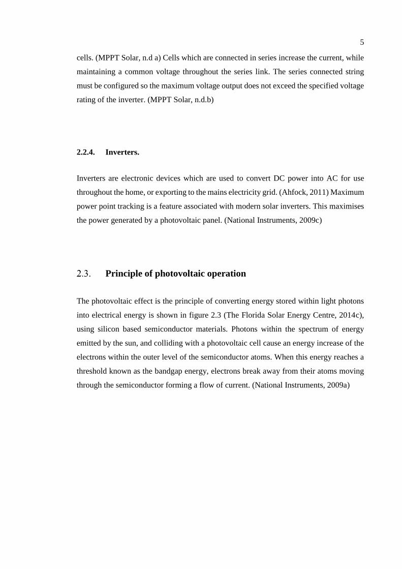
Solar irradiance is a measurement of energy radiated by the sun, measured in watts per
square metre. (Honsberg & Bowden, 2013p) Flat plate solar panels are commonly tested
using a light energy input equal to 1000 watts per square metre and an air mass of 1.5.
(The Florida Solar Energy Centre, 2014a)
Radiated energy which forms part of the electromagnetic spectrum can be described as a
wave with defined wavelength, or a particle of energy called a photon. (Honsberg &
Bowden, 2013o) Only a small region of the electromagnetic spectrum is visible to the
human eye, known as the visible spectrum, and shown in figure 2.4 (Green Rhino Energy
Ltd, 2013). The visible spectrum begins at beginning at a wavelength of approximately
400nm for blue light and ending about 700nm for red light. The energy contained within
photons vary depending on the wavelength as shown in equation 2.1. (Honsberg &
Bowden, 2013o)
Figure 2.4 – Solar radiation and electromagnetic spectrum Green Rhino Energy Ltd, 2013
8
𝐸 = ℎ𝑓 = ℎ𝑐
𝜆 (2.1)
where h is Planck’s constant [ℎ = 6.626 × 10⁻³⁴ 𝐽𝑜𝑢𝑙𝑒. 𝑠];
c is Speed of light in a vacuum [𝑐 = 2.998 × 10⁸ 𝑚. 𝑠−1]; and
λ is the light wavelength (Honsberg & Bowden, 2013h)
Photon flux is a term used to define the density of photons from a light source. The greater
the number of photons being absorbed into the semiconductor material, the higher the
current density within the panel as more electrons available within the conduction band.
Multiplying the photon energy together with the photon flux for a given wavelength will
provide the available energy for such wavelength. (Honsberg & Bowden, 2013n)
Cell size.
The energy transmitted through light is defined as being the total radiated energy in watts,
distributed evenly across a square metre on a plane perpendicular to the direction of light.
The electrical energy generated by the cell will be proportional the area of the collection
area. (Green Rhino Energy Ltd, 2013)
Light angle.
The angle of the light source is a factor which will determine the electrical energy output.
Efficiency of the panel will be at maximum when the light source in perpendicular with
the surface of the panel, and increasing the angle of incidence of the light leads to the
energy being distributed over a larger area, of reduced energy input for the same area.
9
(Green Rhino Energy Ltd, 2013) The factor of this reduction is described by equation 2.2
(Honsberg & Bowden, 2013s)
𝐼(𝜗) = 𝐼𝑜 cos(𝜗) (2.2)
where I is the intensity of the light source and 𝜗 is the angular difference between the
source of light and perpendicular to the panel. (Honsberg & Bowden, 2013s)
The electromagnetic waves emitted by the sun are not polarised, meaning they are random
in rotation about axis of travel. The energy component on the parallel polarisation is
equal to the energy component in the perpendicular polarisation plane. (Howell et al,
2010)
The angle at which light reflected from the surface of an object, and light refracted
through are perpendicular to each other is called the Brewster angle. This is also the angle
at which maximum polarisation will occur. (Encyclopædia Britannica, Inc, 2015a) The
energy available to the cell will be greatly reduced due to the polarising effect. The
Brewster angle can be defined in terms of the refractive indexes of the two medium which
the light is transitioning, and described by equation 2.3. (Howell et al, 2010) Values of
refractive index for air is 1.0002 and for crown glass is 1.517. Encyclopædia Britannica,
Inc, 2015b)
Brewster’s angle 𝜌 = 𝑡𝑎𝑛−1 (𝑛2
𝑛1) (2.3)
Where n is the refractive indexes for each medium.
10
Substitution of the above refraction values into equation 2.3 provides an angle of 56.6°
for light transferring from air into crown glass.
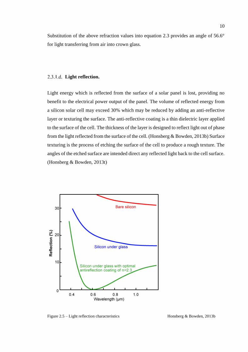
Light reflection.
Light energy which is reflected from the surface of a solar panel is lost, providing no
benefit to the electrical power output of the panel. The volume of reflected energy from
a silicon solar cell may exceed 30% which may be reduced by adding an anti-reflective
layer or texturing the surface. The anti-reflective coating is a thin dielectric layer applied
to the surface of the cell. The thickness of the layer is designed to reflect light out of phase
from the light reflected from the surface of the cell. (Honsberg & Bowden, 2013b) Surface
texturing is the process of etching the surface of the cell to produce a rough texture. The
angles of the etched surface are intended direct any reflected light back to the cell surface.
(Honsberg & Bowden, 2013t)
Figure 2.5 – Light reflection characteristics Honsberg & Bowden, 2013b
11
The level of reflection is shown in Figure 2.5. The use of properly designed reflection
minimisation techniques may reduce the volume of lost energy to negligible levels for a
given light wavelength. (Honsberg & Bowden, 2013b)
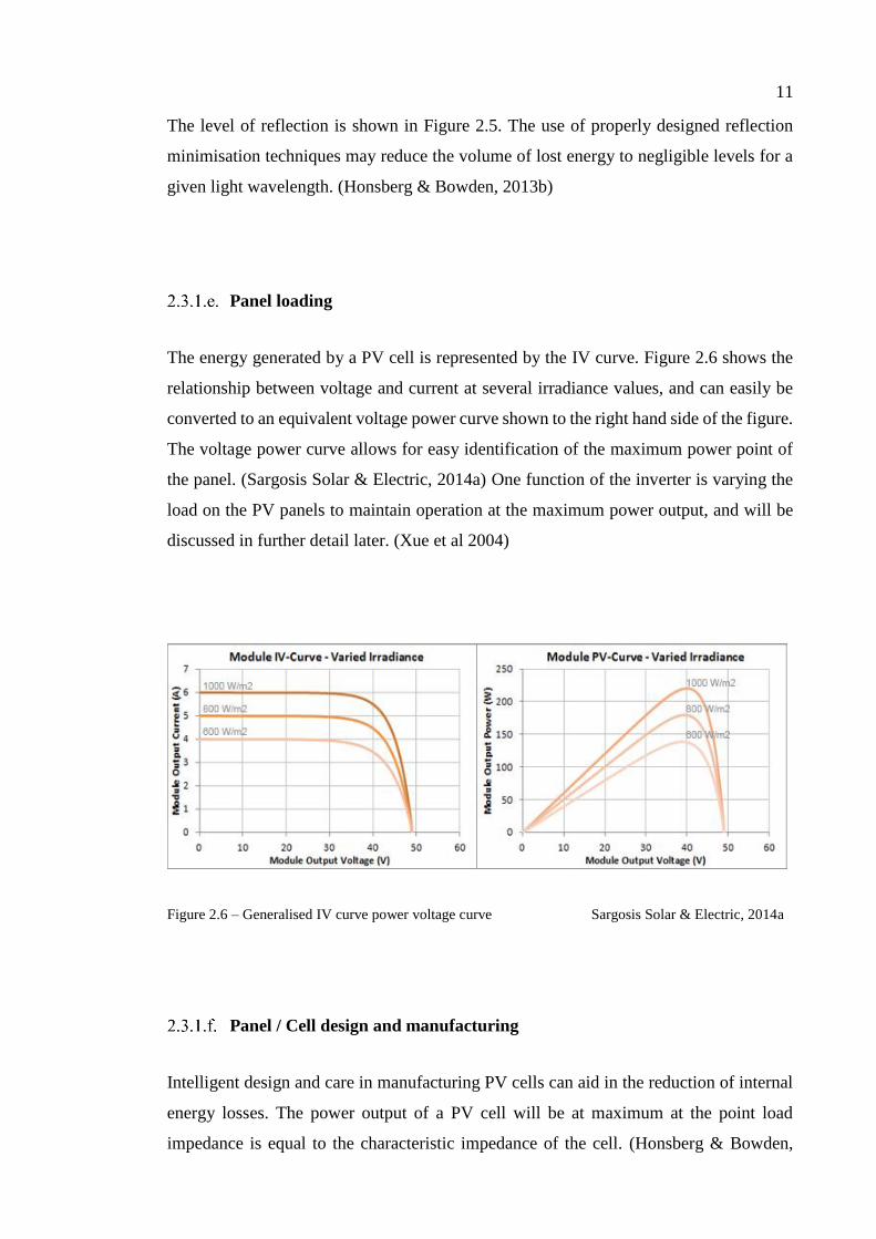
Panel loading
The energy generated by a PV cell is represented by the IV curve. Figure 2.6 shows the
relationship between voltage and current at several irradiance values, and can easily be
converted to an equivalent voltage power curve shown to the right hand side of the figure.
The voltage power curve allows for easy identification of the maximum power point of
the panel. (Sargosis Solar & Electric, 2014a) One function of the inverter is varying the
load on the PV panels to maintain operation at the maximum power output, and will be
discussed in further detail later. (Xue et al 2004)
Figure 2.6 – Generalised IV curve power voltage curve Sargosis Solar & Electric, 2014a
Panel / Cell design and manufacturing
Intelligent design and care in manufacturing PV cells can aid in the reduction of internal
energy losses. The power output of a PV cell will be at maximum at the point load
impedance is equal to the characteristic impedance of the cell. (Honsberg & Bowden,

12
2013d) Parasitic resistance is the term given to the internal series and (shunt) parallel
resistances of a PV cell, reducing the energy output through internal dissipation of power.
(Honsberg & Bowden, 2013e)
Cells which have a low shunt resistance are often the result of manufacturing defects. The
low resistance creates an additional current path, allowing circulating currents to be
generated within the cell. (Honsberg & Bowden, 2013r)
Series resistances are formed by the connection of the semiconductor to the metallic
output contacts, as well as current flow through the cell. The voltage drop caused by a
series resistance will be proportional to the current, therefore the open circuit voltage will
not be affected. (Honsberg & Bowden, 2013q)
Light energy which is reflected, not absorbed or shaded from a PV cell do not add any
value to the output power. Reflection is reduced through the addition of anti-reflective
coatings to the front surface of a PV panel. (Honsberg & Bowden, 2013m) Etching the
front surface of the crystalline wafers produces a rough increases the chance of reflected
light being redirected onto another surface of the cell. (Honsberg & Bowden, 2013t)
Preventing reflection off the rear of the wafer may be achieved by increasing the
thickness, although this may lead to a reduction in the probability the light will generate
a current in the cell. (Honsberg & Bowden, 2013m)
Series connected cells can be affected when the output of one or more cells are reduced.
Under the condition of a short circuit load, shaded or faulty cells will become reverse
biased, dissipating the energy of all other cells as heat. The localised heating may lead to
a burnout within the cell. (Honsberg & Bowden, 2013j) Adding a bypass diode reduced
the reverse bias voltage of a cell, minimising current, and limiting the effect of local heat
dissipation. (Honsberg & Bowden, 2013c)
Circulating currents are formed when differing voltage sources are connected in parallel.
When the output from an individual parallel connected cell is reduced, the chance of
circulating currents is high. Energy from the circulating current is dissipated within the
panel, reducing the power output and potentially damaging the cells. The inclusion of a
current blocking diode in series with each parallel connected the cell eliminates the
chance of circulating currents from occurring. (Pandit & Chaurasia, 2014)
13
Panel shading.
Shading of a photovoltaic cell occurs in two types. Soft shading refers to the reduction of
radiated energy incident on the cell. The cell current will decrease proportionally with the
reduction of the light intensity. The change in cell voltage would be negligible provided
the average irradiance over the entire cell remains above approximately 50 watts per
square metre. (Sargosis Solar & Electric, 2014b)
Hard shading is the complete obstruction of light to an area on the surface of a cell. Cells
which have light exposure forming a path between the electrodes of the cell will generate
the full cell voltage, and a current which is proportionate to the light exposed area. When
a cell is completely covered, the voltage and current output will fail. Shaded cells will
present as a high resistance to the circuit, limiting the output current. (Sargosis Solar &
Electric, 2014b) Current flowing through the high resistance shaded cell will be dissipated
as heat. The localised heating effect could permanently damage the cell. Bypass diodes
provide an alternate path for current protecting the panel and improving efficiency,
effectively removing the non-performing cells from the circuit. The effect of shading on
energy generation may be greater when panels are interconnected. (Solar edge, 2010)
Panel efficiency
Panel efficiency can be described as the percentage of electrical energy produced relative
to the energy contained within the solar radiation. Panels are tested using a set of standard
parameters. (Honsberg & Bowden, 2013g) The energy conversion efficiency will be
affected by the panel design. Efficiencies listed on the Hareon Solar specification sheet
in appendix G range from 11.71% through to 15.40%.
Light power 1000 W/m²
Ambient temperature 25°C
Air mass condition 1.5 (Honsberg & Bowden, 2013g)
14
Panel age
Throughout the lifecycle of a PV cell, the efficiency of the cell to convert solar energy
into electrical energy is reduced. The rate at which degradation occurs is determined by
the construction and materials used to construct the PV cell, as well as the location and
climate in which the cell was to be installed. There is no industry standard on what level
of reduction is required before the cell is deemed to have failed although for most cell
technologies, 20% is considered to be a failure. (Jordan & Kurtz, 2012)
Temperature
Temperature changes affect the energy generated by a solar cell. Increases in temperature
of a cell lead to a reduction of the band gap energy, leading to an increase of the short
circuit current. The intrinsic carrier concentration is determined by the band gap energy,
leading to a reduction in the open circuit voltage of the cell. The result of the change to
the short circuit current and the open circuit voltage is a decrease in output power.
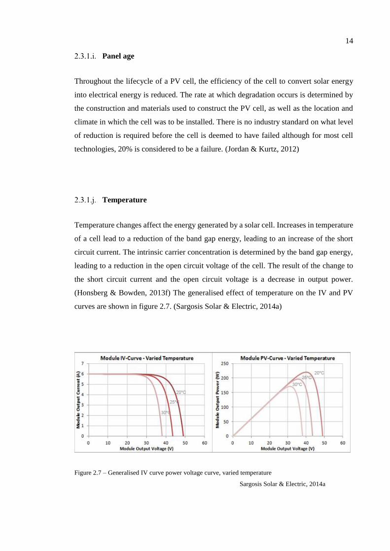
(Honsberg & Bowden, 2013f) The generalised effect of temperature on the IV and PV
curves are shown in figure 2.7. (Sargosis Solar & Electric, 2014a)
Figure 2.7 – Generalised IV curve power voltage curve, varied temperature
Sargosis Solar & Electric, 2014a
15
The temperature coefficients listed for Hareon solar panel models HR190D6P –
HR250D6P,
Pmax -0.44% per 1°C
VOC -0.32% per 1°C
ISC 0.055% per 1°C (Jiangyin Hareon Power Co Ltd, n.d.)
The electrical energy generated by a photovoltaic cell is only a small percentage of the
received solar radiation. Reflected light may account for approximately 4% of the incident
solar radiation, and 5% will be absorbed within the front glass. These losses do not
contribute to the heating of the cells. ((Migan, 2013)The energy converted into electrical
power is dependent on the location on the IV curve and individual panel specifications.
This is commonly around 10 – 15% at the maximum power point, reducing to zero at both
short circuit and open circuit conditions. Remaining solar energy may be absorbed into
the panel, generating internal heating. (Honsberg & Bowden, 2013i)
Heat energy will be lost from the panel into the surrounding environment through three
separate methods. (Honsberg, & Bowden, 2013u) The rate of temperature change will
vary as the differential increases, and will remain constant when the rate of thermal energy
received by the panel is equal to the thermal energy lost. ((Migan, 2013)The angle of the
panes will affect the rate of thermal loss due to convective cooling. The air surrounding
the panel is heated by the panel through convection, which is assisted by the inclined
surface. (Yakoob & Abbas, 2014)
Conduction occurs when the two points of an object are at different temperatures. The
thermal resistance of an object limits the rate of temperature change, creating a
thermal gradient across the object. (Honsberg, & Bowden, 2013u)
Convection is the transfer of heat energy between the surfaces of two objects while in
relative motion. Wind blowing over an object is an example of convection cooling.
Measurement of convection is usually achieved by experimentation as it is often
difficult to calculate. (Honsberg, & Bowden, 2013u)

16
Radiation will be emitted from any object around us. The power of this radiated
energy is determined by the temperature and emissivity of the object. (Honsberg, &
Bowden, 2013u)
Installation design
Mismatch is the situation when one or more cells possess different electrical properties
to the remainder of the cells. The effect of mismatch is a reduction of system efficiency
and potential for permanent damage to the PV cells. There are numerous causes of
mismatch which should be properly assessed during the design of a system, these may
include, connection of non-identical cells and panels, shading of a portion of the PV
system and connection of differently orientated panels. (Honsberg & Bowden, 2013k)
Parallel connection of solar panels is possible provided the following conditions are met,
Panel voltage specifications match,
Panels are installed adjacent and at a common orientation,
Panels are not subject to uneven shading. (MPPT Solar, n.d. a)
Solar cells are commonly connected in series. Cells which have been shaded present a
high resistance to the series connection which may lead to increased heat dissipation. The
inclusion of a bypass diode in parallel with a cell, or group of cells will allow current to
bypass cells which have been shaded. (MPPT Solar, n.d. b)
Air mass
Air mass is a relative value used to account for the energy absorbed by particles within
our atmosphere. As light passes through earths’ atmosphere, air and dust particles absorb
some of the energy. The magnitude of energy absorbed is related to the path length of the
light. (Honsberg & Bowden, 2013a)
17
Inverter design
2.4.1. Introduction to converters.
The development of power electronics has enabled the development of converters which
are devices used to convert an electrical input into a more desirable form. Rectifiers,
inverters and D.C. to D.C. converters are examples of different types of converters.
(Ahfock, 2011)
Rectifiers are used to convert an alternating current input into a direct current output.
The output is dependent on the shape and amplitude of the input. (Ahfock, 2011)
Inverters are used to convert a direct current input into an alternating current output.
The output frequency and voltage are variable. (Ahfock, 2011)
D.C. to D.C. converters are similar to inverters, except the output is direct current.
The voltage is adjustable. (Ahfock, 2011)
2.4.2. Operation of inverters.
Inverters which are commonly used for PV systems normally use a two stage
configuration. The first stage of the inverter is used to boost the input voltage, as well as
maintaining the PV array at the maximum power point. The conversion from D.C. to A.C.
occurs within stage two. (Rosenblatt, L 2015) The inversion process involves the
connection of four transistors in a bridge configuration. Switching specific transistors in
the correct sequence will provide a square wave output. Adjustment of the switching cycle
time and duty cycle will affect the output of the inverter. The addition of frequency filters
and the inductance of the load will assist smoothing of the output waveform. The
characteristics of the transistors will lead to energy losses of the inverter, consisting of
power losses and switching losses. Power losses will be affected by the magnitude of
current, and the impedance of the transistor. Switching losses influenced by the time for
a transistor to switch from off to on and from on to off, as well as the rate at which the
transistor is being switched. (Ahfock, 2011) Single stage inverters perform one voltage
change, while multiple stage inverters will perform a larger number of voltage changes.
(Xue et al 2004)
18
2.4.3. Grid fed inverters.
The connection of a PV array to the public utility grid requires the use of an inverter
capable of converting the variable direct current power generated by the array into a fixed
frequency alternating current supply which is compatible with the grid. This connection
is made possible through the use of a grid fed inverter. (Rosenblatt, L 2015) The function
of a grid fed inverter is more than performing a voltage conversion. Power delivered to
the grid must maintain the same frequency and voltage at the grid while maintaining a
sufficiently low level of harmonic distortion. The inverter must be able to protect
connected equipment against conditions and energy levels which are outside the normal
parameters. (Xue et al 2004)
2.4.4. Single stage inverters.
Single stage inverters provide one point at which voltage change occurs. This stage is
responsible for converting the variable dc input from the array to a fixed frequency power
output which is compatible with the public utility grid supply, in addition to ensuring
isolation between the PV array and the grid and maintaining the operation of the array at
the maximum power point. (Xue et al 2004)
2.4.5. Multiple stage inverters.
Inverters which have more than one stage of voltage change are classed as multiple stage.
A two stage inverter may provide the required electrical isolation, and convert the variable
voltage d.c. from the array into a constant voltage d.c. output. The second stage of the
inverter will be used to generate the a.c. output. There are various multi stage inverter
configurations which can be used for (Xue et al 2004)

19
2.4.6. Inverter efficiency.
The voltage and power generated by a solar string may have an adverse effect on the
efficiency of an inverter. (Folsom Labs, 2014)
Over voltage
The string voltage will be limited by the inverter, preventing any damage due to excessive
voltage levels. When the maximum power point voltage for the string is greater than the
inverter maximum input voltage, the limiting effect causes the string to operate at a
reduced power output. (Folsom Labs, 2014)
Under voltage
Inverters will continue to function if the voltage input falls slightly below the nominal
operating point, although the generated power will be below the maximum power output
of the connected string. Inverters will not function for all voltage levels. Below a
minimum voltage threshold, the power supplied from the panels is insufficient to drive
the circuitry of the inverter. The inverter does not produce any power under this condition.
(Folsom Labs, 2014)
Over power
The design of an inverter includes a maximum power rating, and control to prevent this
situation from occurring. When the supply from a string begins to exceed this rating, the
inverter adjusts the voltage away from the maximum power point, reducing power output.
(Folsom Labs, 2014)

20
Under power
Data provided by the California Energy Commission indicate the efficiency of an inverter
remains relatively constant when the inverter is operating above 30% of full load. The
inverter efficiency reduces as the string power is reduced to between 30 - 10%. (Folsom
Labs, 2014)
2.4.7. Maximum power point tracking.
The power generated by a PV array is dependent on a number of factors, and displayed
by the IV curve. The point on the IV curve where the PV array is greatest is called the
maximum power point. Environmental factors will influence the solar energy input on a
PV array, and hence the output power. The maximum power point does not occur at a
fixed position on the IV curve, therefore is unable to be determined in advance. Maximum
power point tracking is a function included in modern solar inverters, commonly
implemented through constant adjustment of the system operating voltage. There are a
number of methods which can be used to monitor and maintain operation at the maximum
power point. Two methods of maintaining maximum power are perturb and observe and
incremental conductance. (National Instruments, 2009c)
Perturb and observe.
The Perturb and Observe method maintains the output of the array at the maximum power
output by continually monitoring and adjusting the operating voltage or current supplied
by the array. After an adjustment of the operating point of the array, the change in power
determined. When the result is an increase in power, the process is repeated. Likewise
when the result is a decrease in power, the adjustment is performed in the opposite
direction. During steady state operation, the continual adjustment of the operating point
will lead to oscillation about the maximum power point. The simple implementation for
the Perturb and observe method have led to this being the most widely used form of
maximum power point tracking. (National Instruments, 2009c)
21
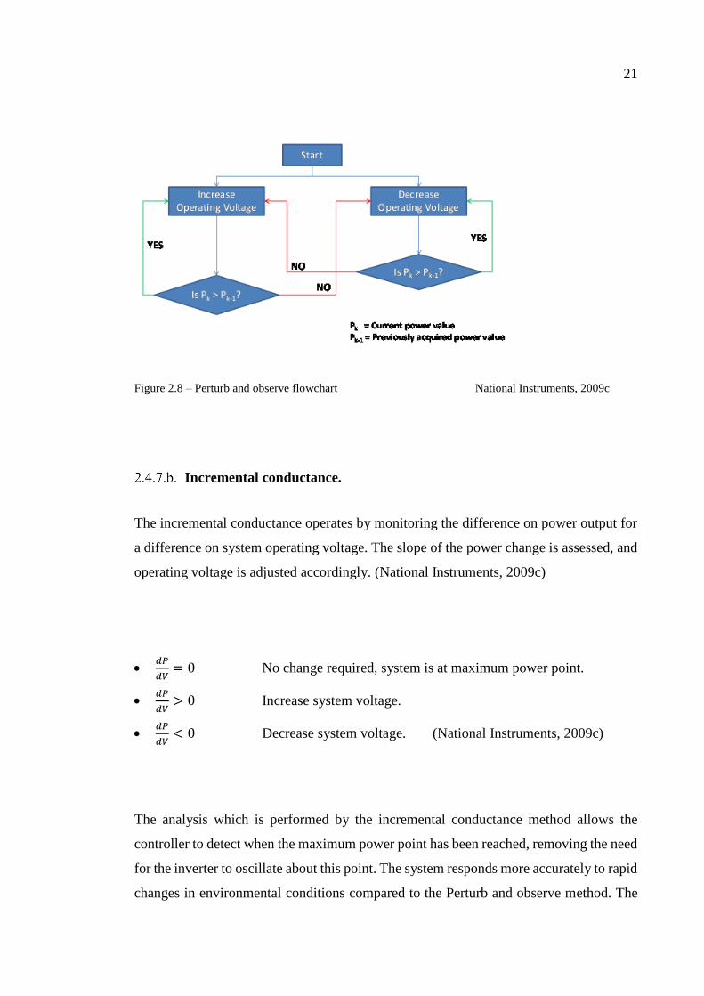
Figure 2.8 – Perturb and observe flowchart National Instruments, 2009c
Incremental conductance.
The incremental conductance operates by monitoring the difference on power output for
a difference on system operating voltage. The slope of the power change is assessed, and
operating voltage is adjusted accordingly. (National Instruments, 2009c)
𝑑𝑃
𝑑𝑉= 0 No change required, system is at maximum power point.
𝑑𝑃
𝑑𝑉> 0 Increase system voltage.
𝑑𝑃
𝑑𝑉< 0 Decrease system voltage. (National Instruments, 2009c)
The analysis which is performed by the incremental conductance method allows the
controller to detect when the maximum power point has been reached, removing the need
for the inverter to oscillate about this point. The system responds more accurately to rapid
changes in environmental conditions compared to the Perturb and observe method. The
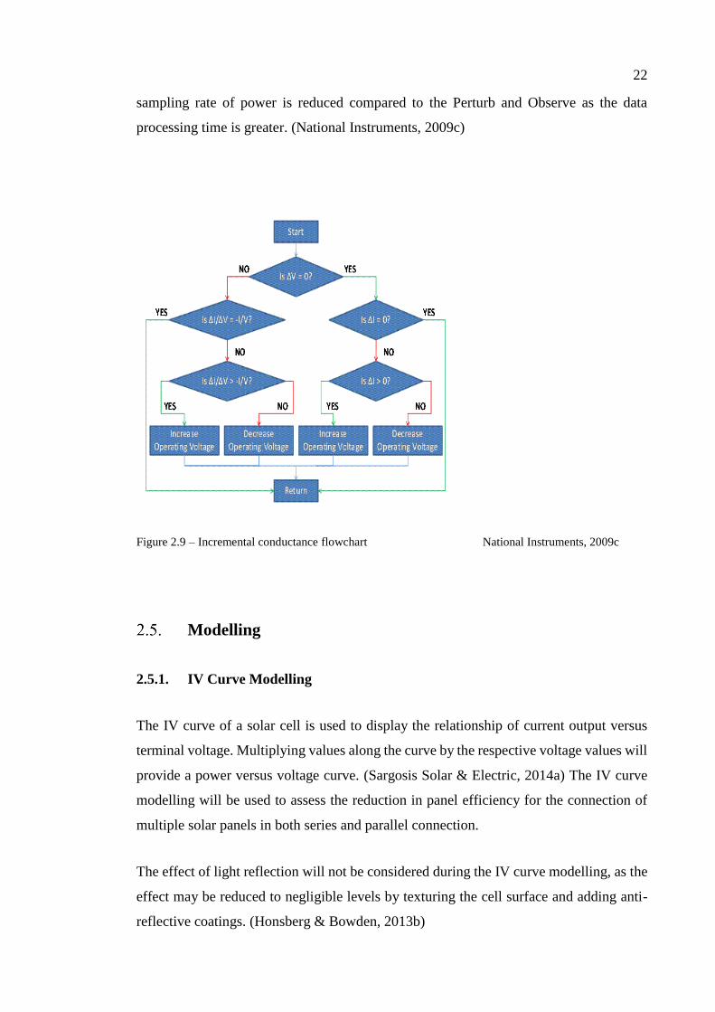
22
sampling rate of power is reduced compared to the Perturb and Observe as the data
processing time is greater. (National Instruments, 2009c)
Figure 2.9 – Incremental conductance flowchart National Instruments, 2009c
Modelling
2.5.1. IV Curve Modelling
The IV curve of a solar cell is used to display the relationship of current output versus
terminal voltage. Multiplying values along the curve by the respective voltage values will
provide a power versus voltage curve. (Sargosis Solar & Electric, 2014a) The IV curve
modelling will be used to assess the reduction in panel efficiency for the connection of
multiple solar panels in both series and parallel connection.
The effect of light reflection will not be considered during the IV curve modelling, as the
effect may be reduced to negligible levels by texturing the cell surface and adding anti-
reflective coatings. (Honsberg & Bowden, 2013b)
23
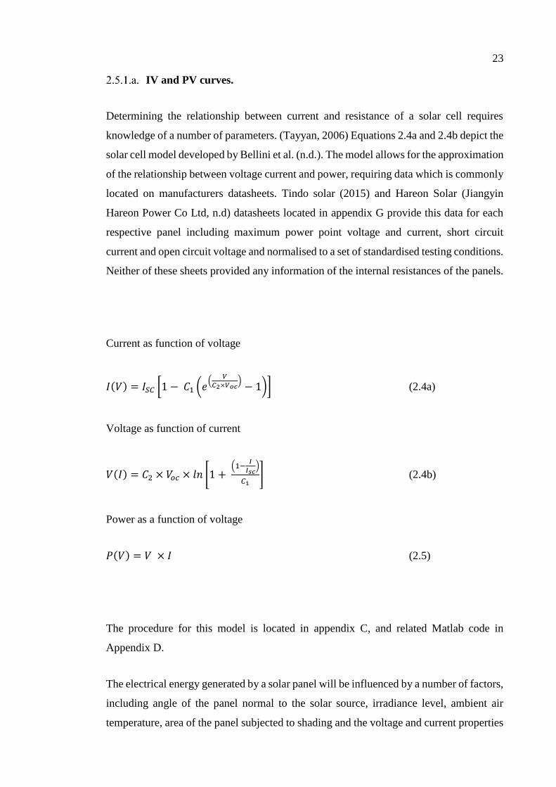
IV and PV curves.
Determining the relationship between current and resistance of a solar cell requires
knowledge of a number of parameters. (Tayyan, 2006) Equations 2.4a and 2.4b depict the
solar cell model developed by Bellini et al. (n.d.). The model allows for the approximation
of the relationship between voltage current and power, requiring data which is commonly
located on manufacturers datasheets. Tindo solar (2015) and Hareon Solar (Jiangyin
Hareon Power Co Ltd, n.d) datasheets located in appendix G provide this data for each
respective panel including maximum power point voltage and current, short circuit
current and open circuit voltage and normalised to a set of standardised testing conditions.
Neither of these sheets provided any information of the internal resistances of the panels.
Current as function of voltage
𝐼(𝑉) = 𝐼𝑆𝐶 [1 − 𝐶1 (𝑒(
𝑉
𝐶2×𝑉𝑜𝑐)
− 1)] (2.4a)
Voltage as function of current
𝑉(𝐼) = 𝐶2 × 𝑉𝑜𝑐 × 𝑙𝑛 [1 + (1−
𝐼
𝐼𝑠𝑐)
𝐶1] (2.4b)
Power as a function of voltage
𝑃(𝑉) = 𝑉 × 𝐼 (2.5)
The procedure for this model is located in appendix C, and related Matlab code in
Appendix D.
The electrical energy generated by a solar panel will be influenced by a number of factors,
including angle of the panel normal to the solar source, irradiance level, ambient air
temperature, area of the panel subjected to shading and the voltage and current properties

24
of the individual panel. The IV curve modelling will be used to assess the efficiency of a
system with multiple panels connected in either series or parallel while subjected to
different input influences. Equation 2.4a will be used with a common voltage vector to
model parallel connected systems, and equation 2.4b will be used for series connected
systems with a common current vector. Equation 2.5 will be used to form a power vector.
Location of maximum power point.
The process to identify the maximum power point will be derived from the Perturb and
observe method as stated by National Instruments (2009c). The voltage vector will be
checked for a value matching the calculated maximum power point voltage. The value of
the corresponding position on the power vector will be checked and assessed against both
adjacent values, indexing the position to the highest value of power. When the selected
value of power is greater than both adjacent values, the program loop will be terminated.

25
3. Project planning.
The successful completion of any major is heavily influenced by the project planning
conducted through the early stages of the project. During this phase, the project planner
should divide the overall project down into a smaller set of tasks, and develop a
methodology for the project completion. Consideration must also be given to the required
resources, and their availability. The inclusion of a timeline for the completion of
specified tasks will assist in maintaining the project to be completed by the required
deadline. (ENG4111 Research project part 1: Project reference book, 2014)
Ethics.
The intention of this project is to improve the annual energy generated by new
photovoltaic installations throughout Australia. The installation parameters detailed
within are intended to comply with all regulatory requirements, as well as the
requirements of the Engineers Australia code of ethics.
Methodology.
The steps required for the investigation of different solar panel and inverter
configurations, and the development of optimised installation parameters will be detailed
within the following methodology section.
3.2.1. Required resources.
MATLAB is a text based computer programming language, specialising in numerical,
signal and image processing. The language commonly used throughout various

26
engineering disciplines, as custom scripts can be written to perform repeated calculations.
(Palm, 2009)
Designed by the National Renewable Energy Laboratory, Homer is a software modelling
tool specialising in the optimisation of electrical microrgids. The package has the
capability to model a variety of supply source options and load profiles. Simulations are
conducted to cover each combination of design elements, providing an analysis for the
energy generation and consumption together with financial details for each system design
option. (Homer Energy, 2015)
3.2.2. Identification and sourcing of relevant literature.
The accuracy of the sourced information is an important factor to maintain the integrity
of the finished project. Inaccurate or misleading information may possibly lead to an
invalid course of investigation, even an unsubstantiated final outcome. (ENG4111
Research project part 1: Project reference book, 2014)
During the search for information, there will be an emphasis on information sources
where the author/s are associated with educational institutions or government. This is
intended to remove a potential source of bias, focussing more on information provided
by non-commercial sources.
3.2.3. Modelling multiple interconnected solar panels.
The relationship between voltage, current and power will be calculated within MATLAB
using the IV curve approximation detailed in appendix C. The combined output from
multiple energy sources can be determined by summing the voltage or current for series
or parallel connections respectively. The simulation was used to calculate the IV curve
for each individual panel, reflecting the output under specific instantaneous installation
conditions. The resulting currents will be added along a common voltage vector for
parallel and voltage on common current for series connection, along with corresponding

27
power curves. The slope of each power curve generated are analysed to identify the
localised maximum power value. The angle of one panel is indexed, test repeated and
power values recorded forming a power to vector relative to angular offset. The resulting
information is intended to provide an understanding into the energy losses which are
likely to occur when multiple connected panels are installed at differing angles.
3.2.4. Modelling solar panel optimum angle.
Homer Energy will be used to determine the energy produced by a solar energy system
with panels orientated at a variety of azimuth and tilt angles at four location throughout
Australia. In the first stage of modelling, the azimuth will be assessed at 15° intervals
over a complete 360° range, and tilt at 15° intervals and a 90° range. This stage is intended
to demonstrate the effect of azimuth and tilt have on the annual energy production of solar
systems. The second modelling stage will assess the azimuth and tilt angles over a smaller
range at 1° intervals. Energy generation data from Homer will be used to identify the tilt
angle providing the highest energy yield over the azimuth vector. The derivation of a
polynomial curve function requires knowledge of certain points on the curve. (Larson &
Falvo, 2009) The optimum azimuth variable and longitude for each site will form the
optimum azimuth function, while the optimum tilt and the site latitude will be used for
the tilt function.
28
3.2.5. Modelling multiple string systems.
Annual energy generation for multi string systems will be determined using Homer. The
different inverter configurations will be used for the multi string simulations.
Single inverter with single channel maximum power point tracking
Single inverter with dual channel maximum power point tracking
Two inverters, each with single channel maximum power point tracking
Data extracted from the Homer simulations will be used to determine the conditions
required for specific inverter configurations. Changes in different installation angles will
also be assessed to determine if the optimum installation angles identified for single string
systems can be applied to multiple string systems.
3.2.6. Selection of installation locations.
Multiple sites were selected ranging from Darwin, Northern Territory as a northern
location through to Hobart, Tasmania as a southern location. Toowoomba, Queensland
and Brooklyn Park, South Australia were included as intermediate locations. The
optimum angle of installation is to be determined for each site using solar data available
through the Homer energy modelling software, and temperature data from the Australian
Bureau of Meteorology for the year 2014. Sites were selected to provide a range of
locations covering a large portion of the country, weather data available nearby.
29
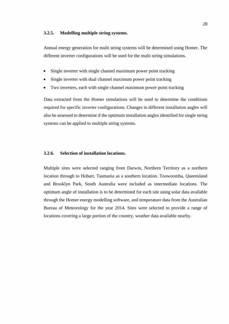
Brooklyn Park, S.A.
Site: Brooklyn Apartments, Brooklyn Park.
Location: 34.93°S, 138.55°E (Google, 2015)
Weather data site: 34.95°S, 138.52°E. (Commonwealth of Australia, 2015)
Brooklyn Park is a suburb of Adelaide, located approximately 5km west if the city.
Located on approximately 5km south west is the Bureau of meteorology weather
monitoring station, providing historic temperature data. (Google, 2015)
Figure 3.1 – Brooklyn Park site overview Google, 2015
Building Azimuth: 177°
30
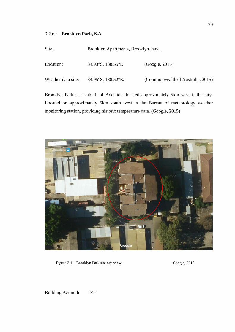
Toowoomba, Qld.
Site: USQ, Toowoomba: Engineering (Z block)
Location: 27.60°S, 151.93°E (Google, 2015)
Weather data site: 27.54°S, 151.91°E. (Commonwealth of Australia, 2015)
The University of Southern Queensland is located in Toowoomba, approximately 125km
east by road from the city of Brisbane. Approximately 10km north of the university is the
site of the Bureau of Meteorology weather monitoring station. (Google, 2015)
Figure 3.2 – Toowoomba site overview Google, 2015
Building Azimuth 195° / 217° / 246°
31
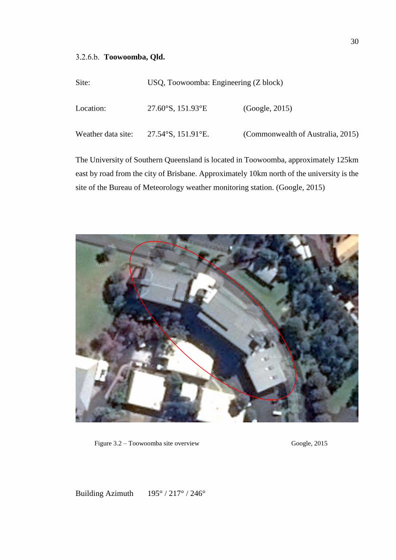
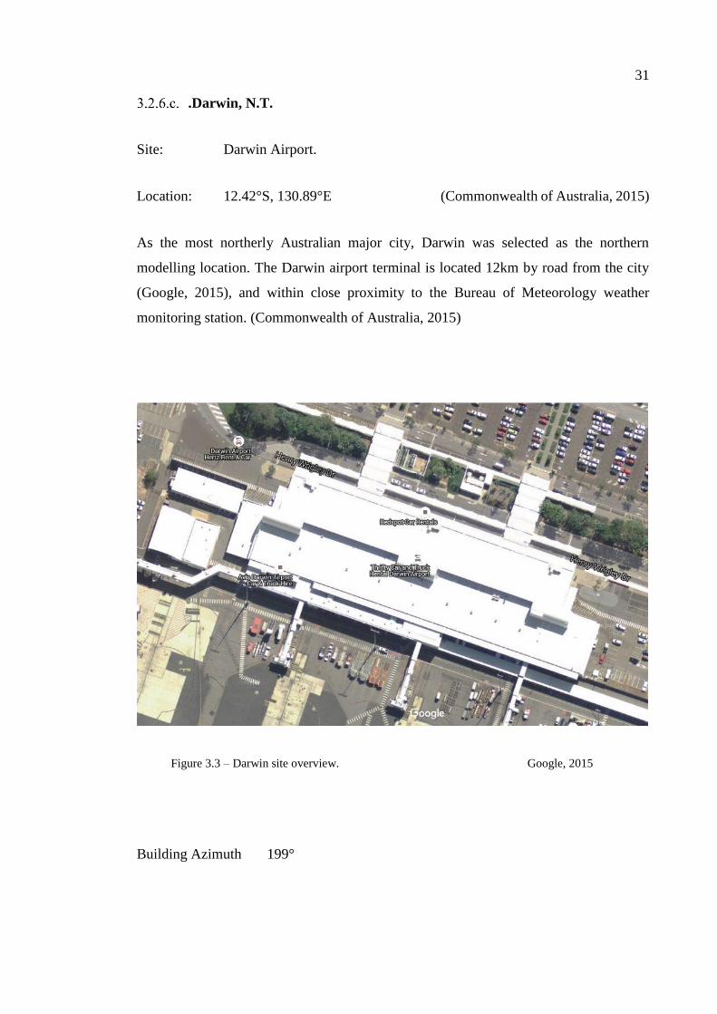
.Darwin, N.T.
Site: Darwin Airport.
Location: 12.42°S, 130.89°E (Commonwealth of Australia, 2015)
As the most northerly Australian major city, Darwin was selected as the northern
modelling location. The Darwin airport terminal is located 12km by road from the city
(Google, 2015), and within close proximity to the Bureau of Meteorology weather
monitoring station. (Commonwealth of Australia, 2015)
Figure 3.3 – Darwin site overview. Google, 2015
Building Azimuth 199°
32
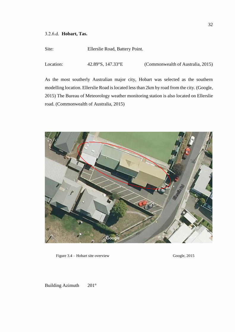
Hobart, Tas.
Site: Ellerslie Road, Battery Point.
Location: 42.89°S, 147.33°E (Commonwealth of Australia, 2015)
As the most southerly Australian major city, Hobart was selected as the southern
modelling location. Ellerslie Road is located less than 2km by road from the city. (Google,
2015) The Bureau of Meteorology weather monitoring station is also located on Ellerslie
road. (Commonwealth of Australia, 2015)
Figure 3.4 – Hobart site overview Google, 2015
Building Azimuth 201°

33
3.2.7. Panel angle effect on cooling.
The effect panel tilt angle has on the convective cooling will be determined through
experimentation.
1. The panel should remain open circuit throughout this experiment.
2. Ensure panel is sheltered from wind.
3. Align the panel to 0° relative to horizontal.
4. Record cell temperature using FLIR thermal camera
5. Repeat cell temperature measurement every 5 minutes until steady state is
reached.
6. Align panel to an angle greater than 0° and repeat test steps 2 through 5
The global solar irradiance available from the USQ weather station, combined with the
angle of the sun relative to the panel will be used to calculate the panel energy input.
The cell temperature rise values recorded using the FLIR camera will then be used to
determine the cell temperature. Since cell temperature is a function of the irradiance, the
resulting values can be scaled to reflect a solar irradiance value of 1000W/m². ((Migan,
2013)A line of best fit will used to be approximate the angle versus temperature rise and
related efficiency decrease, with the resulting efficiency changes factored into the Homer
modelling outputs.
3.2.8. Development of installation guidelines.
The modelling process is expected to generate a large amount of energy output data. The
data will need to be analysed to identify the parameters which provide the greatest energy
yields, and will be used to form the basis for the recommended installation guidelines.

34
Parameters which will be included in the final recommendations are listed below.
Preferred inverter configurations.
This will detail the best inverter configuration which should be selected for a range
of solar panel installation parameters.
Maximum permissible angles between strings on the same maximum power point
tracking circuit.
This details the maximum installation azimuth and tilt angles which should be
permitted if two strings are connected to a common maximum power point tracking
circuit.
Optimum tilt angles for the installation of solar panels.
The use of renewable energies, and reduction of fossil fuel generated power should could
lead to a Greenhouse Installing solar panels at angles which provide the largest annual
energy generation a greater annual generation The optimum angle for installation will be
used to define the best panel tilt angle for a range of azimuth angles. , providing maximum
power.
Project timeline.
Some of the major project milestones are listed below, and a detailed project
timeline is located in appendix B.
Completion of project allocation
Completion of Project specification
Selection of potential sites
Completion of IV curve modelling
Commencement of site modelling
Submission of project preliminary report
Project completion

35
Assessment of consequential effects.
The work health safety act require health and safety be maintained through the
identification of safety hazards. If the elimination of a safety hazard is not possible, the
risk must be reduced to as safe level as possible. (Safe work Australia, 2011) Used under
a Creative Commons Attribution 3.0 (http://creativecommons.org/licenses/by-
nc/3.0/au/).
Responsibility for the effective implementation of risk elimination and control is
normally initiated by company management, although does extend to all persons on site.
(Safe work Australia, 2011) Used under a Creative Commons Attribution 3.0
(http://creativecommons.org/licenses/by-nc/3.0/au/).
The risk management process consists of four steps.
i. Identify any hazard associated with the project.
ii. Assess the risk of all identified hazards, including details on seriousness of injury
if an accident were to occur, and the chance of an accident occurring.
iii. Determine the required measures to eliminate or reduce the severity of the risk,
and implement the solution.
iv. Review the risk management measures which have been implemented to ensure
effectiveness of the solution, and new hazards have not been introduced.
(Safe work Australia, 2011) Used under a Creative Commons Attribution 3.0
(http://creativecommons.org/licenses/by-nc/3.0/au/).
During the risk management, the work health safety act also requires an appropriate level
of consultation with any person who may be affected by the work carried out. (Safe work
Australia, 2011) Used under a Creative Commons Attribution 3.0
(http://creativecommons.org/licenses/by-nc/3.0/au/)

36
3.4.1. Identification of hazards.
Identification of hazards is simply an analysis of a product, process or situation which has
the potential to cause harm to any person. This may require an observation of a specific
processes being conducted, consultation with workers regarding near misses or an
assessment of a piece of equipment being commissioned. (Safe work Australia, 2011)
Used under a Creative Commons Attribution 3.0
(http://creativecommons.org/licenses/by-nc/3.0/au/).
3.4.2. Risk assessment.
Following the identification of potential hazards, each hazard is then assessed for the
potential to cause harm. The risk assessment may assist in determining the severity of a
potential risk, effectiveness of current risk mitigation measures, what corrective action is
most appropriate and urgency of the urgency of corrective action. (Safe work Australia,
2011) Used under a Creative Commons Attribution 3.0
(http://creativecommons.org/licenses/by-nc/3.0/au/).
Risk assessments should be conducted prior to the introduction of a new piece of
equipment, modification to existing processes, when there is no information of the risk of
a specific task or equipment, or how specific hazards will interact. (Safe work Australia,
2011) Used under a Creative Commons Attribution 3.0
(http://creativecommons.org/licenses/by-nc/3.0/au/).

37
3.4.3. Risk matrix scores.
The overall risk is then identified using a scoring system. Each hazard is assessed, and
assigned an individual score for time of exposure to the hazard, chance of an accident
occurring and the potential consequence if an accident were to occur. (University of
Melbourne, 2004)
Tables relating to the risk assessment scores can be located in Appendix F.
3.4.4. Risk assessment outcomes.
Following the assignment of the risk scores, control measured need to be identified for
each of the hazard. (University of Melbourne, 2004)
Control measures should be selected for each hazard in a hierarchical manner,
1. Elimination of the hazard
2. Substitution of the process with a reduced risk process.
3. Providing a barrier between the worker and the hazard in the form of guarding or
fencing.
4. Engineering controls include the use of mechanical aids to reduce manual
handling, or setting work output requirements to a level which is more suited to
the task.
5. Administrative controls include the introduction of work processes designed to
reduce the workers exposure to certain hazards, or informing workers of the
potential hazard.
6. Requiring the use of personal protective equipment.

38
Steps 5 & 6 should only be used when all other possible solutions have been
exhausted, or as a short term control measure until more suitable measures can be
introduced. (Safe work Australia, 2011) Used under a Creative Commons Attribution
3.0 (http://creativecommons.org/licenses/by-nc/3.0/au/).
3.4.5. Project hazard identification and risk assessment.
Hazard identification and risk assessments which have been conducted for this project are
located in Appendix F.

39
4. Results
IV Curve modelling.
The photovoltaic panel specifications, and environmental input specifications used
throughout the modelling were from the Hareon Solar model HR-250W, which has a
maximum power output of 250W under standard test conditions. (Jiangyin Hareon Power
Co Ltd, n.d.)
Maximum power voltage 29.90V
Open circuit voltage 37.10V
Maximum power current 8.36A
Short circuit current 8.81A
Irradiance 1000W/m²
Ambient temperature 25°C (Jiangyin Hareon Power Co Ltd, n.d.)
No shading on the panel surface.
Full specifications are available in appendix G.
The above specification have been used throughout each modelling section, unless
otherwise specified.
The modelling consisted of two photovoltaic panels connected in parallel, or in series and
compared to the benchmark condition. Panel 1 was set at a fixed angle with a normal
vector relative to the light source. Panel 2 was set with the normal facing the light source,
and rotated through to 56° during the simulation. Each panel consisted of three modules
with bypass diode, and the panel was fitted with a blocking diode.
This section is intended to compare the effect of differing panel angles on the maximum
power generated. The benchmark for maximum power capability used throughout the
modelling is the sum total of maximum power capabilities with the same installation
parameters. This is to compare the effect of offset panel angles on the maximum power
capability, irrespective of the installation or environmental conditions.
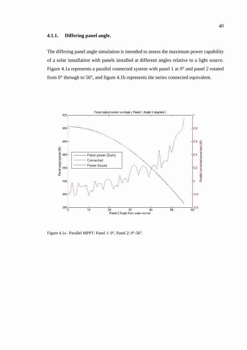
40
4.1.1. Differing panel angle.
The differing panel angle simulation is intended to assess the maximum power capability
of a solar installation with panels installed at different angles relative to a light source.
Figure 4.1a represents a parallel connected system with panel 1 at 0° and panel 2 rotated
from 0° through to 56°, and figure 4.1b represents the series connected equivalent.
Figure 4.1a –Parallel MPPT: Panel 1: 0°, Panel 2: 0°-56°.
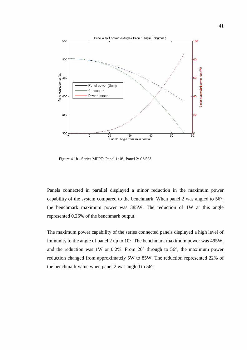
41
Figure 4.1b –Series MPPT: Panel 1: 0°, Panel 2: 0°-56°.
Panels connected in parallel displayed a minor reduction in the maximum power
capability of the system compared to the benchmark. When panel 2 was angled to 56°,
the benchmark maximum power was 385W. The reduction of 1W at this angle
represented 0.26% of the benchmark output.
The maximum power capability of the series connected panels displayed a high level of
immunity to the angle of panel 2 up to 10°. The benchmark maximum power was 495W,
and the reduction was 1W or 0.2%. From 20° through to 56°, the maximum power
reduction changed from approximately 5W to 85W. The reduction represented 22% of
the benchmark value when panel 2 was angled to 56°.
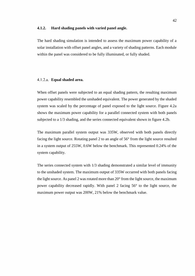
42
4.1.2. Hard shading panels with varied panel angle.
The hard shading simulation is intended to assess the maximum power capability of a
solar installation with offset panel angles, and a variety of shading patterns. Each module
within the panel was considered to be fully illuminated, or fully shaded.
Equal shaded area.
When offset panels were subjected to an equal shading pattern, the resulting maximum
power capability resembled the unshaded equivalent. The power generated by the shaded
system was scaled by the percentage of panel exposed to the light source. Figure 4.2a
shows the maximum power capability for a parallel connected system with both panels
subjected to a 1/3 shading, and the series connected equivalent shown in figure 4.2b.
The maximum parallel system output was 335W, observed with both panels directly
facing the light source. Rotating panel 2 to an angle of 56° from the light source resulted
in a system output of 255W, 0.6W below the benchmark. This represented 0.24% of the
system capability.
The series connected system with 1/3 shading demonstrated a similar level of immunity
to the unshaded system. The maximum output of 335W occurred with both panels facing
the light source. As panel 2 was rotated more than 20° from the light source, the maximum
power capability decreased rapidly. With panel 2 facing 56° to the light source, the
maximum power output was 200W, 21% below the benchmark value.
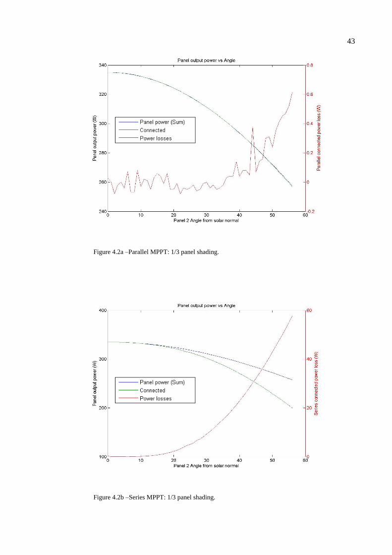
43
Figure 4.2a –Parallel MPPT: 1/3 panel shading.
Figure 4.2b –Series MPPT: 1/3 panel shading.
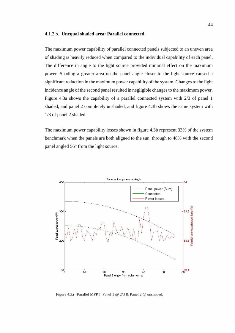
44
Unequal shaded area: Parallel connected.
The maximum power capability of parallel connected panels subjected to an uneven area
of shading is heavily reduced when compared to the individual capability of each panel.
The difference in angle to the light source provided minimal effect on the maximum
power. Shading a greater area on the panel angle closer to the light source caused a
significant reduction in the maximum power capability of the system. Changes to the light
incidence angle of the second panel resulted in negligible changes to the maximum power.
Figure 4.3a shows the capability of a parallel connected system with 2/3 of panel 1
shaded, and panel 2 completely unshaded, and figure 4.3b shows the same system with
1/3 of panel 2 shaded.
The maximum power capability losses shown in figure 4.3b represent 33% of the system
benchmark when the panels are both aligned to the sun, through to 48% with the second
panel angled 56° from the light source.
Figure 4.3a –Parallel MPPT: Panel 1 @ 2/3 & Panel 2 @ unshaded.
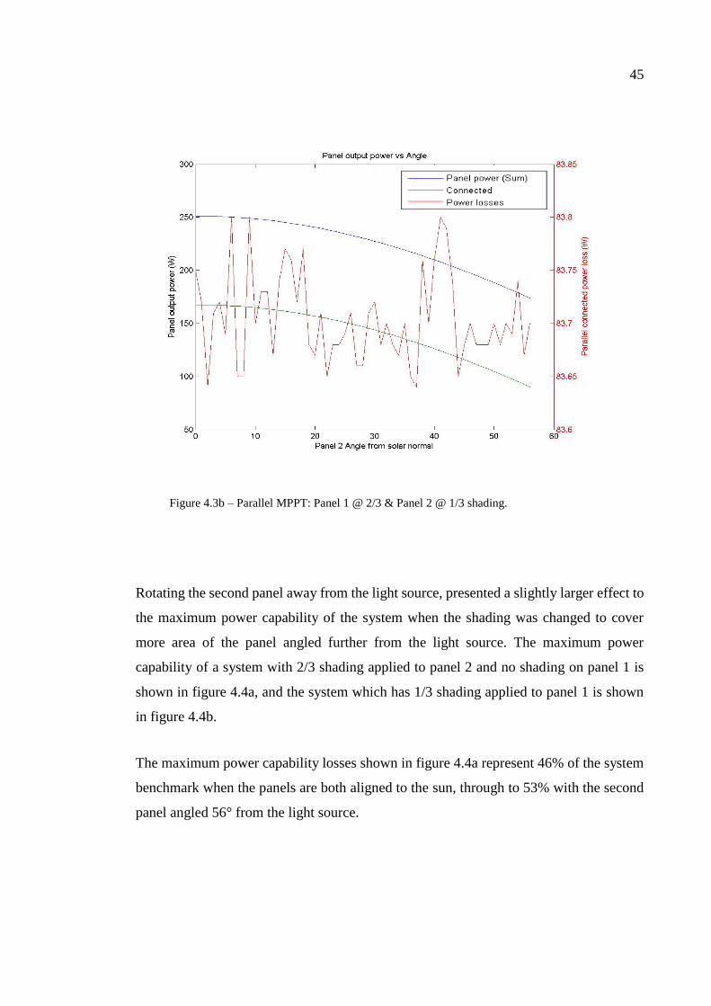
45
Figure 4.3b – Parallel MPPT: Panel 1 @ 2/3 & Panel 2 @ 1/3 shading.
Rotating the second panel away from the light source, presented a slightly larger effect to
the maximum power capability of the system when the shading was changed to cover
more area of the panel angled further from the light source. The maximum power
capability of a system with 2/3 shading applied to panel 2 and no shading on panel 1 is
shown in figure 4.4a, and the system which has 1/3 shading applied to panel 1 is shown
in figure 4.4b.
The maximum power capability losses shown in figure 4.4a represent 46% of the system
benchmark when the panels are both aligned to the sun, through to 53% with the second
panel angled 56° from the light source.
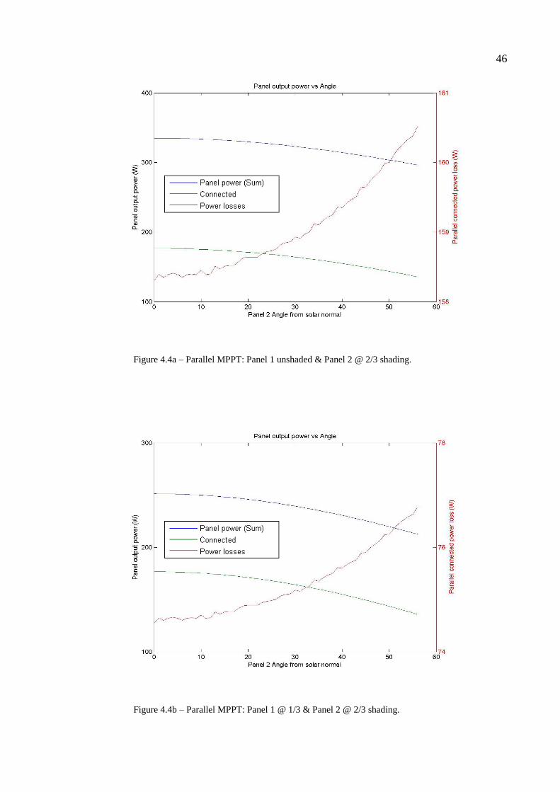
46
Figure 4.4a – Parallel MPPT: Panel 1 unshaded & Panel 2 @ 2/3 shading.
Figure 4.4b – Parallel MPPT: Panel 1 @ 1/3 & Panel 2 @ 2/3 shading.
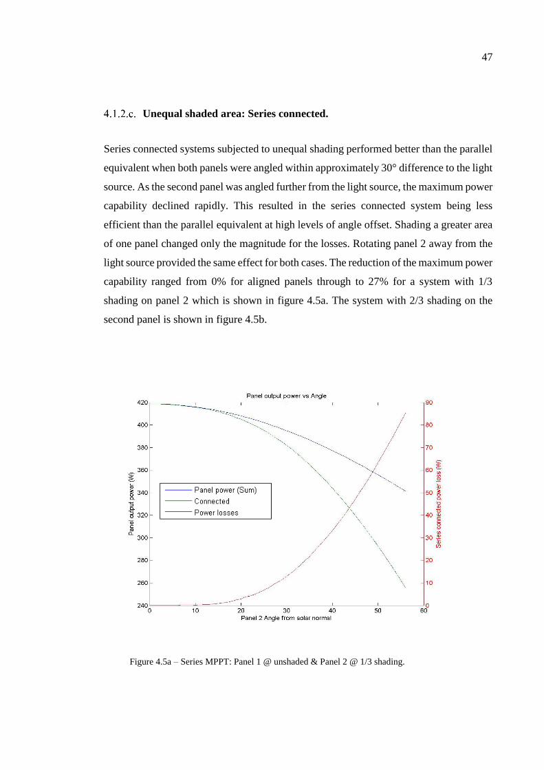
47
Unequal shaded area: Series connected.
Series connected systems subjected to unequal shading performed better than the parallel
equivalent when both panels were angled within approximately 30° difference to the light
source. As the second panel was angled further from the light source, the maximum power
capability declined rapidly. This resulted in the series connected system being less
efficient than the parallel equivalent at high levels of angle offset. Shading a greater area
of one panel changed only the magnitude for the losses. Rotating panel 2 away from the
light source provided the same effect for both cases. The reduction of the maximum power
capability ranged from 0% for aligned panels through to 27% for a system with 1/3
shading on panel 2 which is shown in figure 4.5a. The system with 2/3 shading on the
second panel is shown in figure 4.5b.
Figure 4.5a – Series MPPT: Panel 1 @ unshaded & Panel 2 @ 1/3 shading.
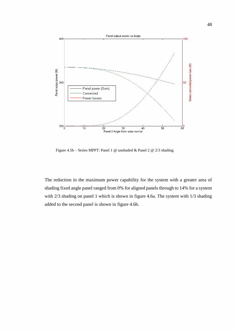
48
Figure 4.5b – Series MPPT: Panel 1 @ unshaded & Panel 2 @ 2/3 shading.
The reduction in the maximum power capability for the system with a greater area of
shading fixed angle panel ranged from 0% for aligned panels through to 14% for a system
with 2/3 shading on panel 1 which is shown in figure 4.6a. The system with 1/3 shading
added to the second panel is shown in figure 4.6b.
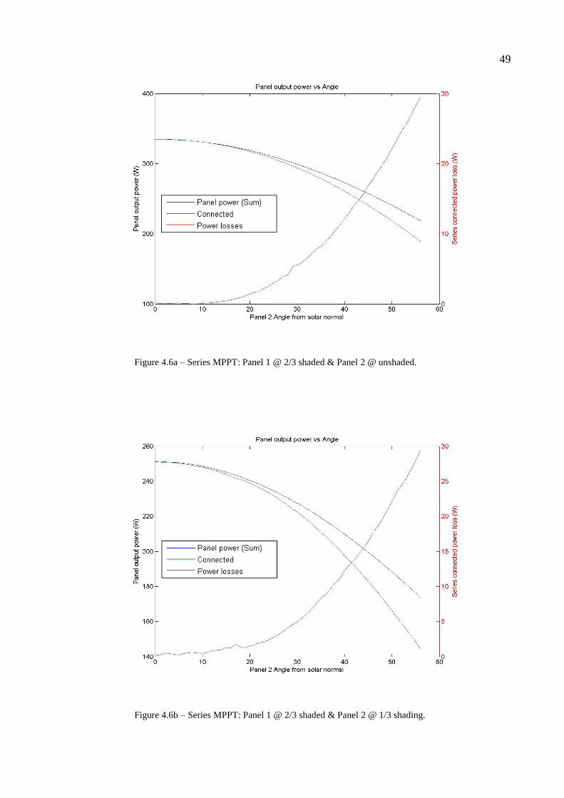
49
Figure 4.6a – Series MPPT: Panel 1 @ 2/3 shaded & Panel 2 @ unshaded.
Figure 4.6b – Series MPPT: Panel 1 @ 2/3 shaded & Panel 2 @ 1/3 shading.
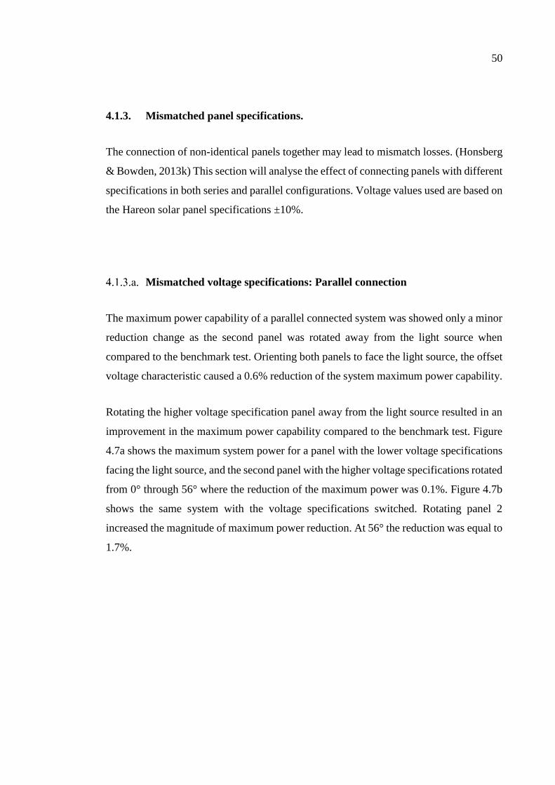
50
4.1.3. Mismatched panel specifications.
The connection of non-identical panels together may lead to mismatch losses. (Honsberg
& Bowden, 2013k) This section will analyse the effect of connecting panels with different
specifications in both series and parallel configurations. Voltage values used are based on
the Hareon solar panel specifications ±10%.
Mismatched voltage specifications: Parallel connection
The maximum power capability of a parallel connected system was showed only a minor
reduction change as the second panel was rotated away from the light source when
compared to the benchmark test. Orienting both panels to face the light source, the offset
voltage characteristic caused a 0.6% reduction of the system maximum power capability.
Rotating the higher voltage specification panel away from the light source resulted in an
improvement in the maximum power capability compared to the benchmark test. Figure
4.7a shows the maximum system power for a panel with the lower voltage specifications
facing the light source, and the second panel with the higher voltage specifications rotated
from 0° through 56° where the reduction of the maximum power was 0.1%. Figure 4.7b
shows the same system with the voltage specifications switched. Rotating panel 2
increased the magnitude of maximum power reduction. At 56° the reduction was equal to
1.7%.
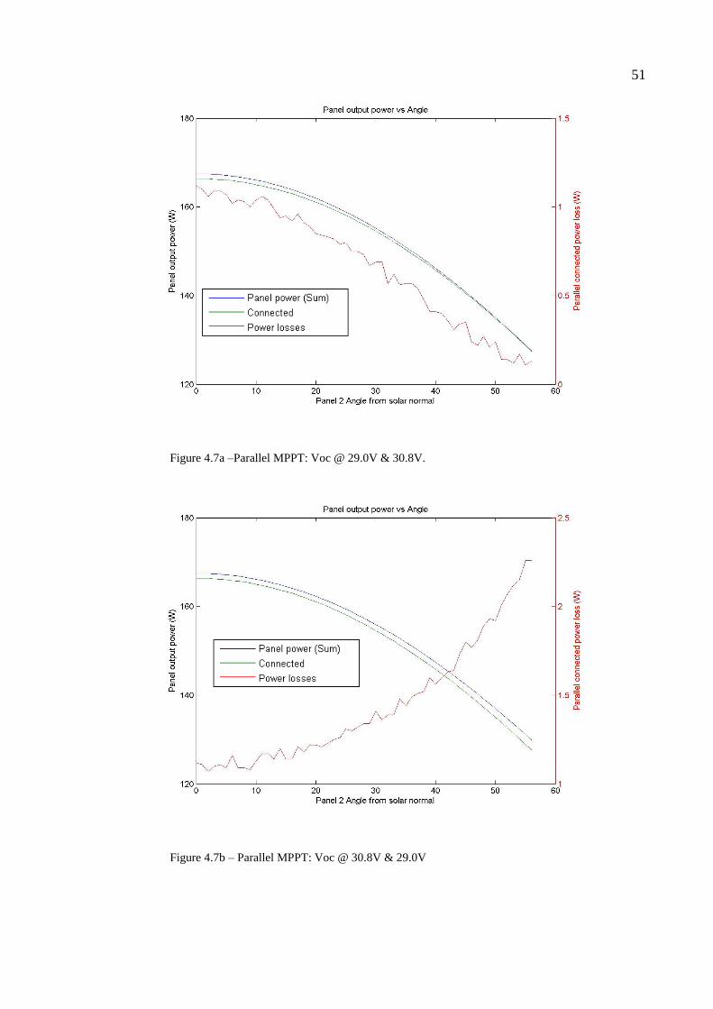
51
Figure 4.7a –Parallel MPPT: Voc @ 29.0V & 30.8V.
Figure 4.7b – Parallel MPPT: Voc @ 30.8V & 29.0V
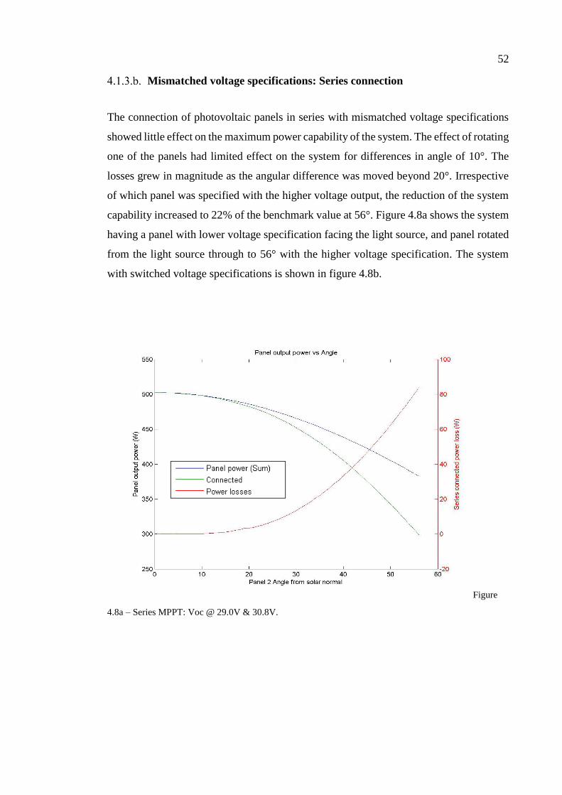
52
Mismatched voltage specifications: Series connection
The connection of photovoltaic panels in series with mismatched voltage specifications
showed little effect on the maximum power capability of the system. The effect of rotating
one of the panels had limited effect on the system for differences in angle of 10°. The
losses grew in magnitude as the angular difference was moved beyond 20°. Irrespective
of which panel was specified with the higher voltage output, the reduction of the system
capability increased to 22% of the benchmark value at 56°. Figure 4.8a shows the system
having a panel with lower voltage specification facing the light source, and panel rotated
from the light source through to 56° with the higher voltage specification. The system
with switched voltage specifications is shown in figure 4.8b.
Figure
4.8a – Series MPPT: Voc @ 29.0V & 30.8V.
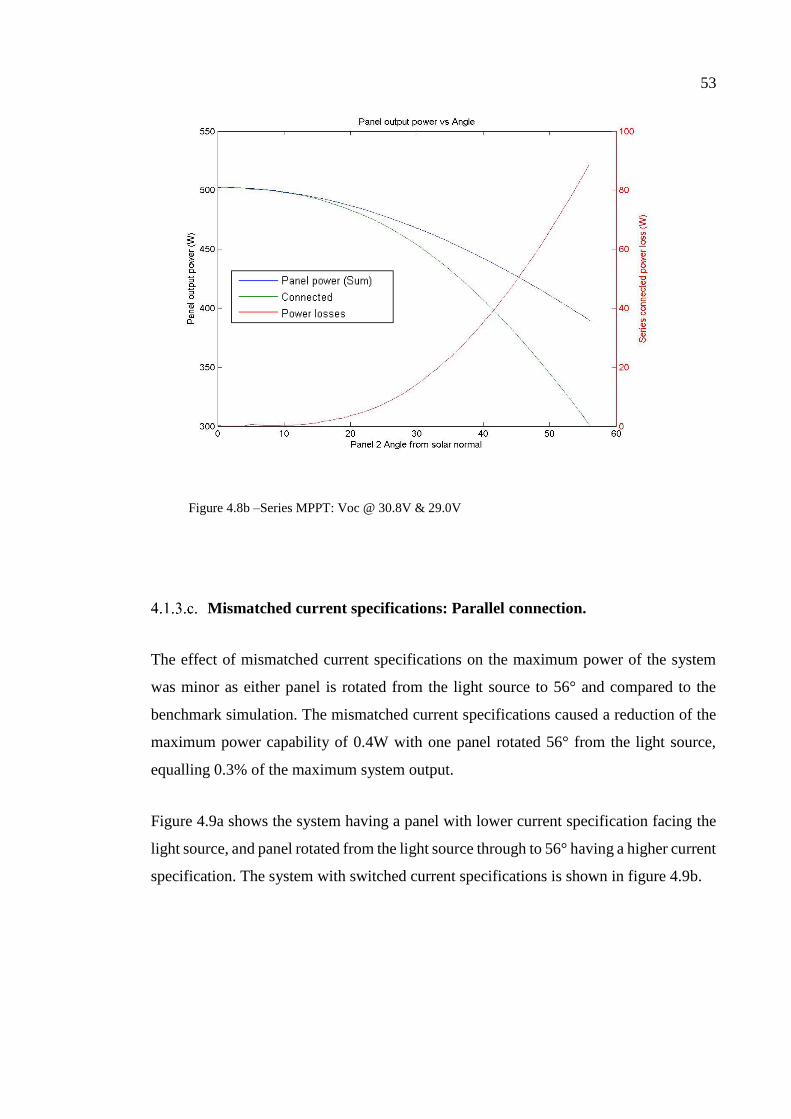
53
Figure 4.8b –Series MPPT: Voc @ 30.8V & 29.0V
Mismatched current specifications: Parallel connection.
The effect of mismatched current specifications on the maximum power of the system
was minor as either panel is rotated from the light source to 56° and compared to the
benchmark simulation. The mismatched current specifications caused a reduction of the
maximum power capability of 0.4W with one panel rotated 56° from the light source,
equalling 0.3% of the maximum system output.
Figure 4.9a shows the system having a panel with lower current specification facing the
light source, and panel rotated from the light source through to 56° having a higher current
specification. The system with switched current specifications is shown in figure 4.9b.
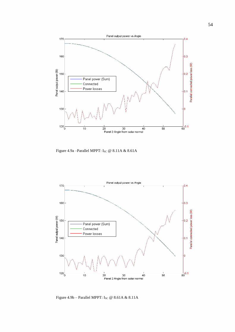
54
Figure 4.9a –Parallel MPPT: ISC @ 8.11A & 8.61A
Figure 4.9b – Parallel MPPT: ISC @ 8.61A & 8.11A
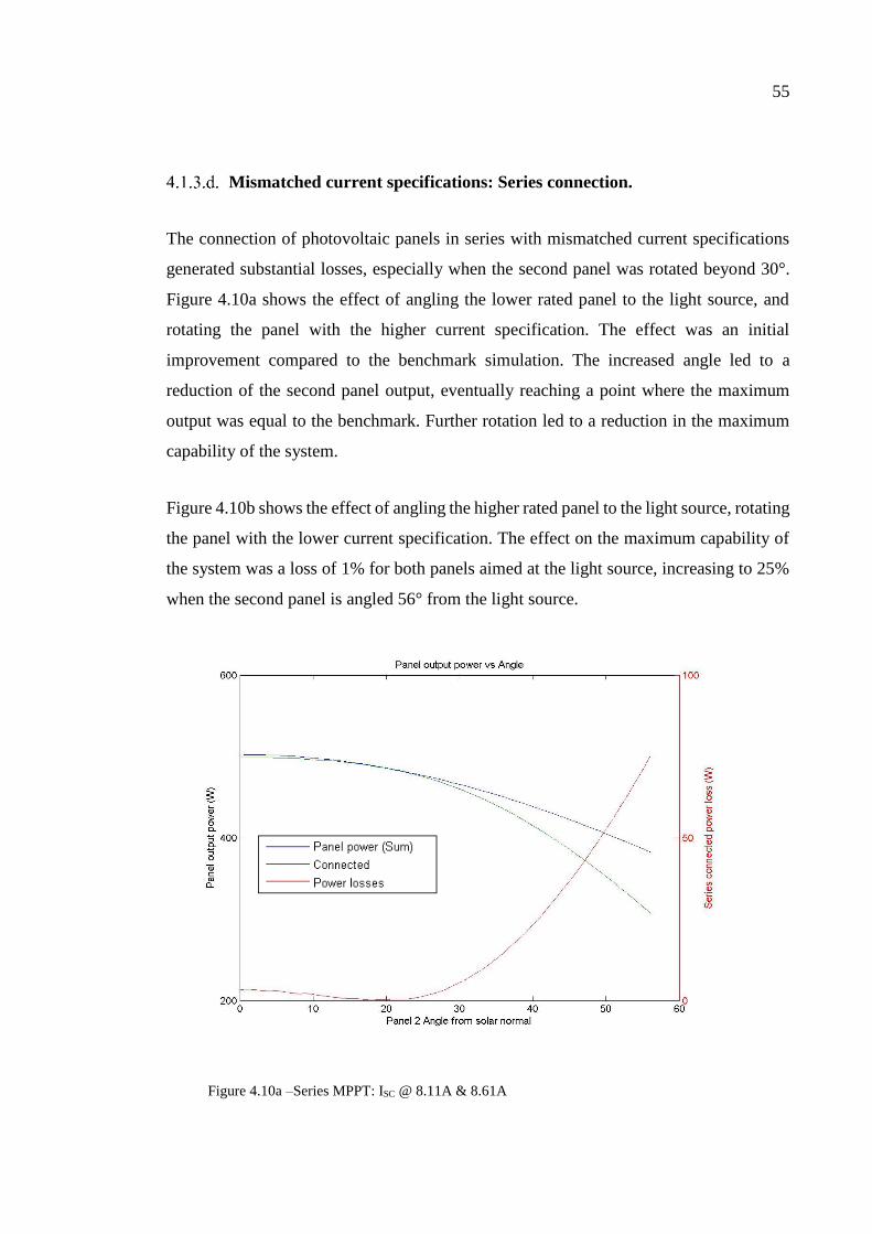
55
Mismatched current specifications: Series connection.
The connection of photovoltaic panels in series with mismatched current specifications
generated substantial losses, especially when the second panel was rotated beyond 30°.
Figure 4.10a shows the effect of angling the lower rated panel to the light source, and
rotating the panel with the higher current specification. The effect was an initial
improvement compared to the benchmark simulation. The increased angle led to a
reduction of the second panel output, eventually reaching a point where the maximum
output was equal to the benchmark. Further rotation led to a reduction in the maximum
capability of the system.
Figure 4.10b shows the effect of angling the higher rated panel to the light source, rotating
the panel with the lower current specification. The effect on the maximum capability of
the system was a loss of 1% for both panels aimed at the light source, increasing to 25%
when the second panel is angled 56° from the light source.
Figure 4.10a –Series MPPT: ISC @ 8.11A & 8.61A
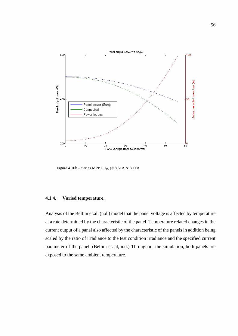
56
Figure 4.10b – Series MPPT: ISC @ 8.61A & 8.11A
4.1.4. Varied temperature.
Analysis of the Bellini et.al. (n.d.) model that the panel voltage is affected by temperature
at a rate determined by the characteristic of the panel. Temperature related changes in the
current output of a panel also affected by the characteristic of the panels in addition being
scaled by the ratio of irradiance to the test condition irradiance and the specified current
parameter of the panel. (Bellini et. al, n.d.) Throughout the simulation, both panels are
exposed to the same ambient temperature.
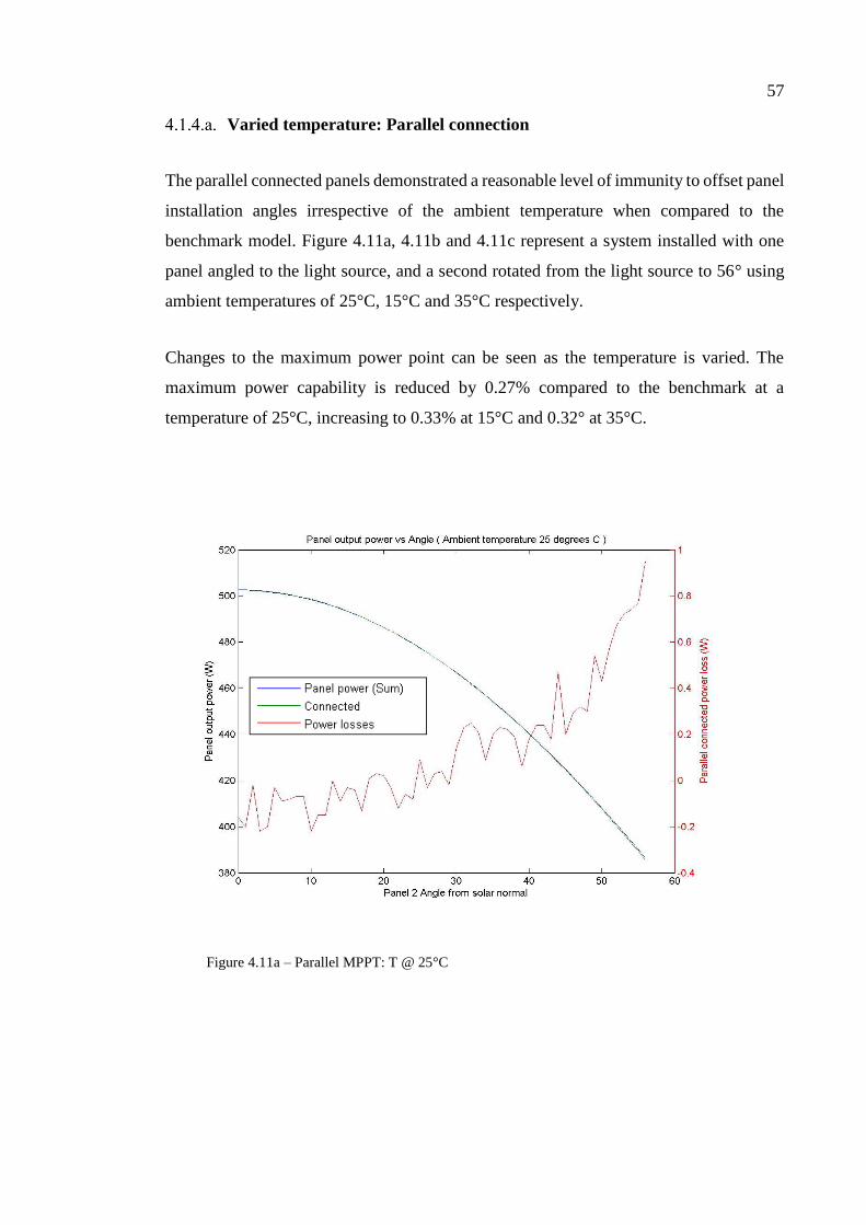
57
Varied temperature: Parallel connection
The parallel connected panels demonstrated a reasonable level of immunity to offset panel
installation angles irrespective of the ambient temperature when compared to the
benchmark model. Figure 4.11a, 4.11b and 4.11c represent a system installed with one
panel angled to the light source, and a second rotated from the light source to 56° using
ambient temperatures of 25°C, 15°C and 35°C respectively.
Changes to the maximum power point can be seen as the temperature is varied. The
maximum power capability is reduced by 0.27% compared to the benchmark at a
temperature of 25°C, increasing to 0.33% at 15°C and 0.32° at 35°C.
Figure 4.11a – Parallel MPPT: T @ 25°C
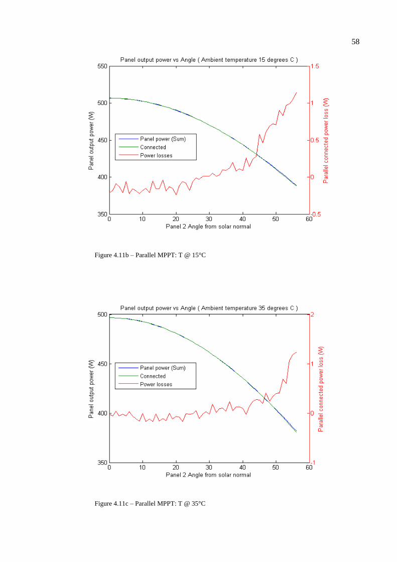
58
Figure 4.11b – Parallel MPPT: T @ 15°C
Figure 4.11c – Parallel MPPT: T @ 35°C
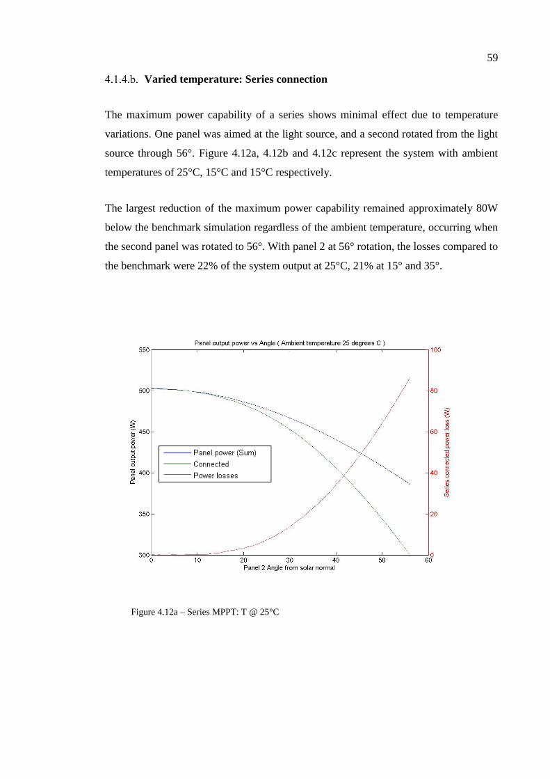
59
Varied temperature: Series connection
The maximum power capability of a series shows minimal effect due to temperature
variations. One panel was aimed at the light source, and a second rotated from the light
source through 56°. Figure 4.12a, 4.12b and 4.12c represent the system with ambient
temperatures of 25°C, 15°C and 15°C respectively.
The largest reduction of the maximum power capability remained approximately 80W
below the benchmark simulation regardless of the ambient temperature, occurring when
the second panel was rotated to 56°. With panel 2 at 56° rotation, the losses compared to
the benchmark were 22% of the system output at 25°C, 21% at 15° and 35°.
Figure 4.12a – Series MPPT: T @ 25°C
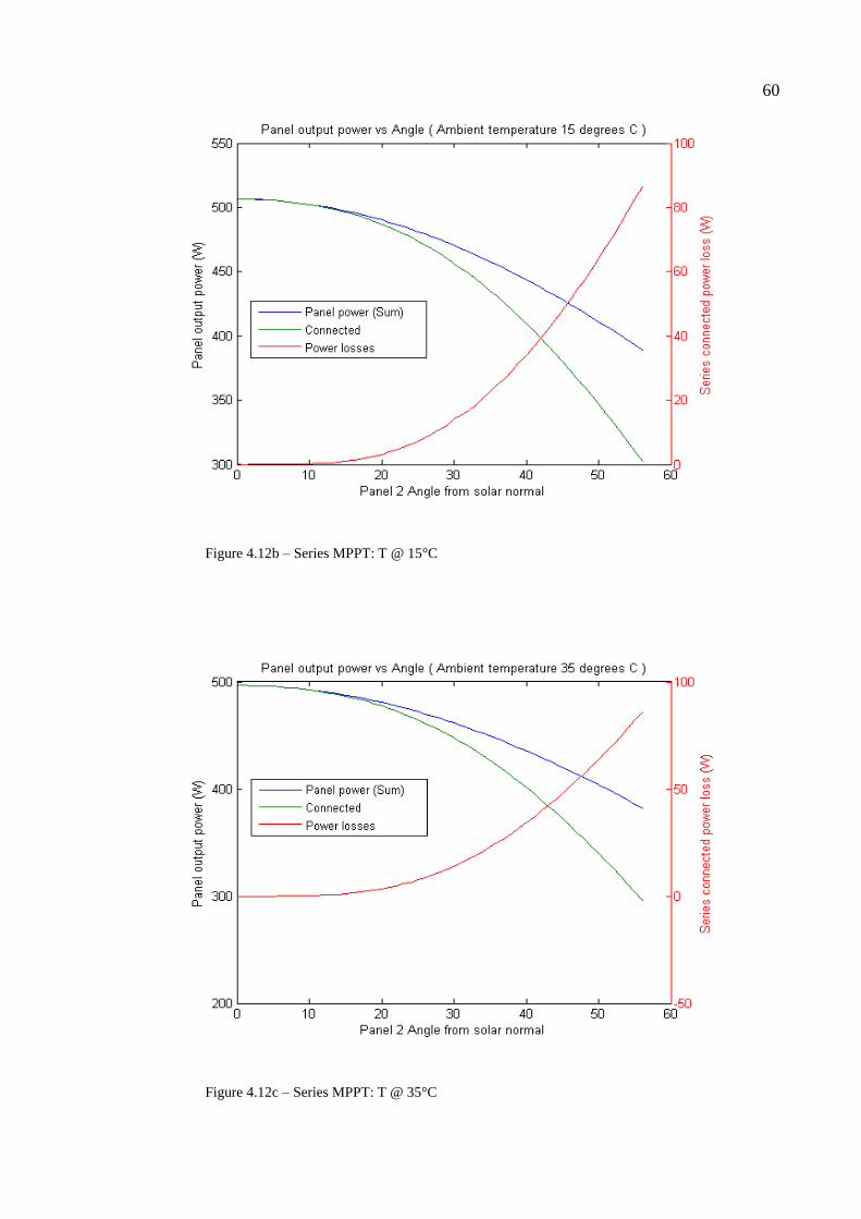
60
Figure 4.12b – Series MPPT: T @ 15°C
Figure 4.12c – Series MPPT: T @ 35°C
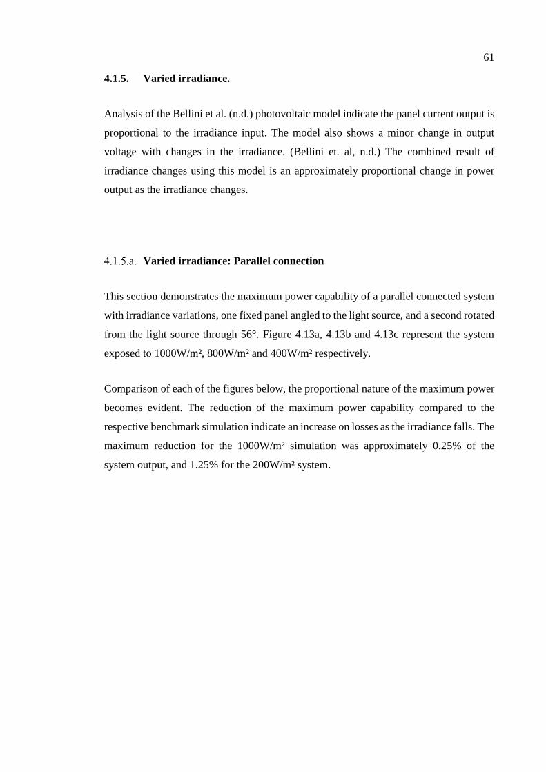
61
4.1.5. Varied irradiance.
Analysis of the Bellini et al. (n.d.) photovoltaic model indicate the panel current output is
proportional to the irradiance input. The model also shows a minor change in output
voltage with changes in the irradiance. (Bellini et. al, n.d.) The combined result of
irradiance changes using this model is an approximately proportional change in power
output as the irradiance changes.
Varied irradiance: Parallel connection
This section demonstrates the maximum power capability of a parallel connected system
with irradiance variations, one fixed panel angled to the light source, and a second rotated
from the light source through 56°. Figure 4.13a, 4.13b and 4.13c represent the system
exposed to 1000W/m², 800W/m² and 400W/m² respectively.
Comparison of each of the figures below, the proportional nature of the maximum power
becomes evident. The reduction of the maximum power capability compared to the
respective benchmark simulation indicate an increase on losses as the irradiance falls. The
maximum reduction for the 1000W/m² simulation was approximately 0.25% of the
system output, and 1.25% for the 200W/m² system.
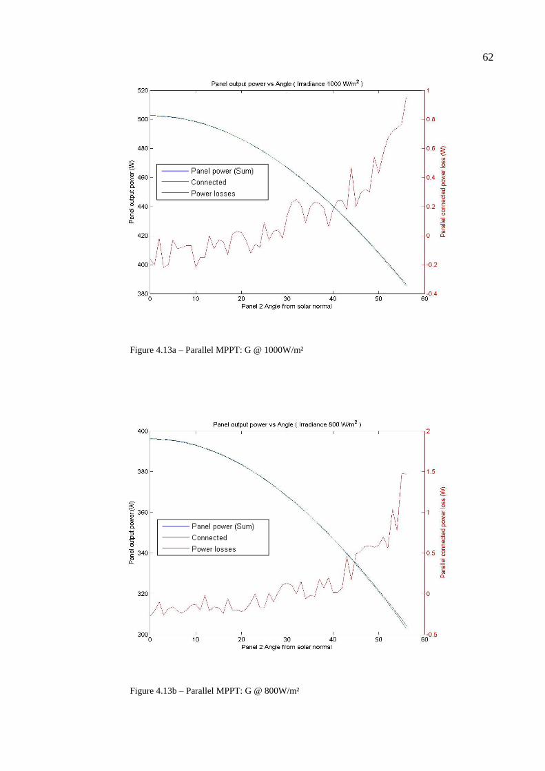
62
Figure 4.13a – Parallel MPPT: G @ 1000W/m²
Figure 4.13b – Parallel MPPT: G @ 800W/m²
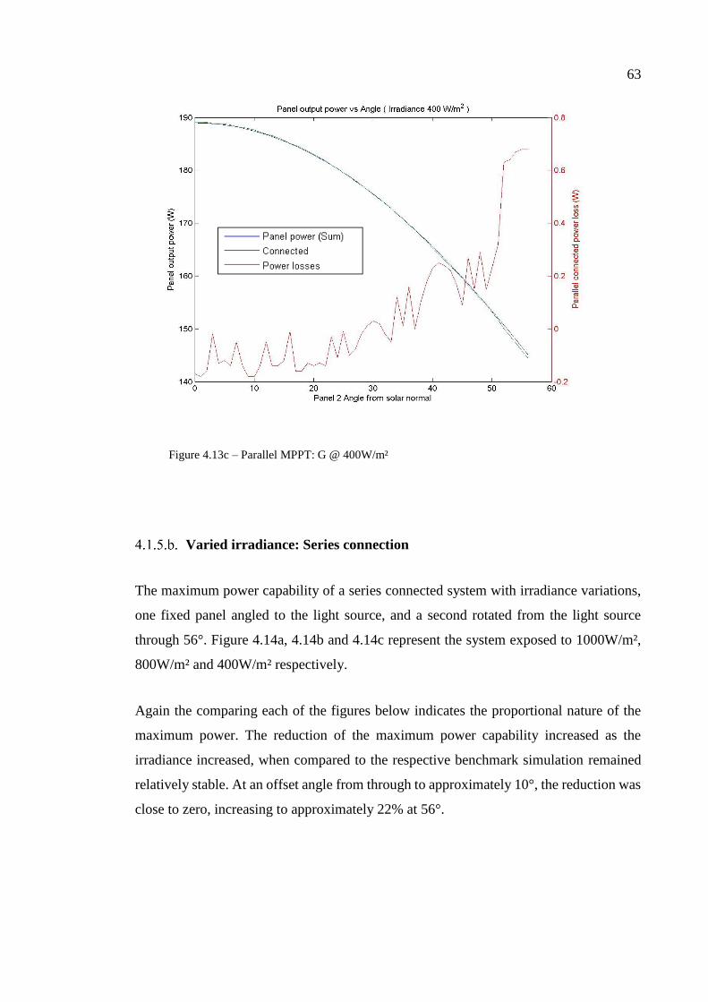
63
Figure 4.13c – Parallel MPPT: G @ 400W/m²
Varied irradiance: Series connection
The maximum power capability of a series connected system with irradiance variations,
one fixed panel angled to the light source, and a second rotated from the light source
through 56°. Figure 4.14a, 4.14b and 4.14c represent the system exposed to 1000W/m²,
800W/m² and 400W/m² respectively.
Again the comparing each of the figures below indicates the proportional nature of the
maximum power. The reduction of the maximum power capability increased as the
irradiance increased, when compared to the respective benchmark simulation remained
relatively stable. At an offset angle from through to approximately 10°, the reduction was
close to zero, increasing to approximately 22% at 56°.
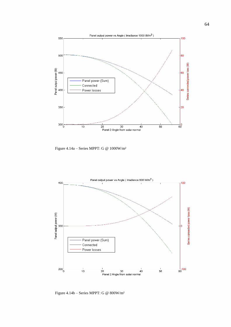
64
Figure 4.14a – Series MPPT: G @ 1000W/m²
Figure 4.14b – Series MPPT: G @ 800W/m²
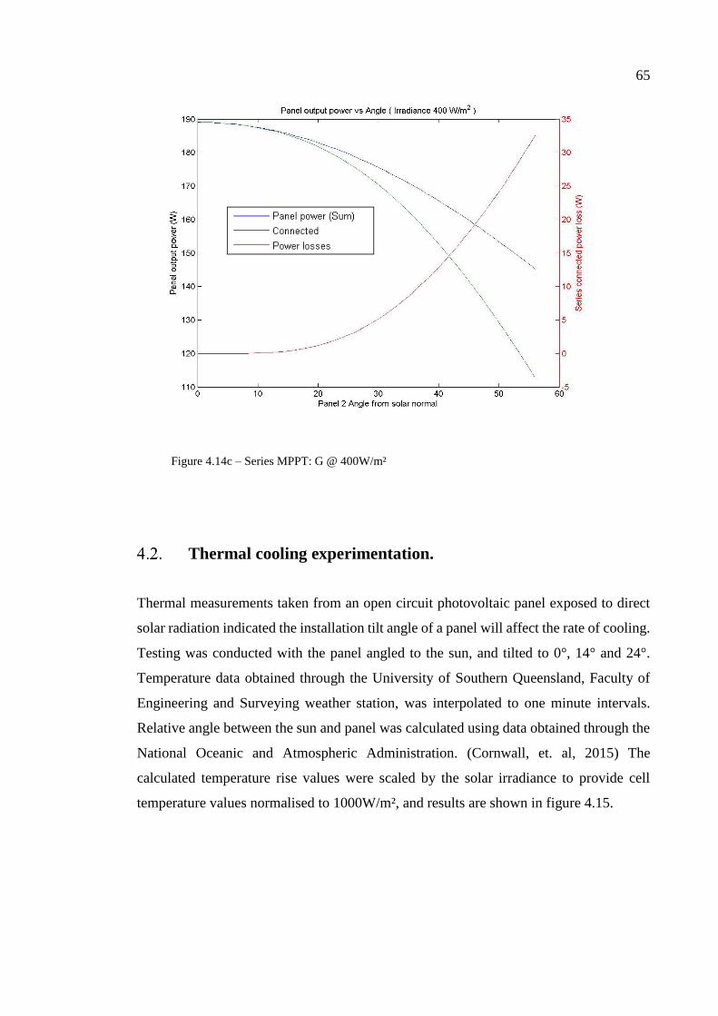
65
Figure 4.14c – Series MPPT: G @ 400W/m²
Thermal cooling experimentation.
Thermal measurements taken from an open circuit photovoltaic panel exposed to direct
solar radiation indicated the installation tilt angle of a panel will affect the rate of cooling.
Testing was conducted with the panel angled to the sun, and tilted to 0°, 14° and 24°.
Temperature data obtained through the University of Southern Queensland, Faculty of
Engineering and Surveying weather station, was interpolated to one minute intervals.
Relative angle between the sun and panel was calculated using data obtained through the
National Oceanic and Atmospheric Administration. (Cornwall, et. al, 2015) The
calculated temperature rise values were scaled by the solar irradiance to provide cell
temperature values normalised to 1000W/m², and results are shown in figure 4.15.
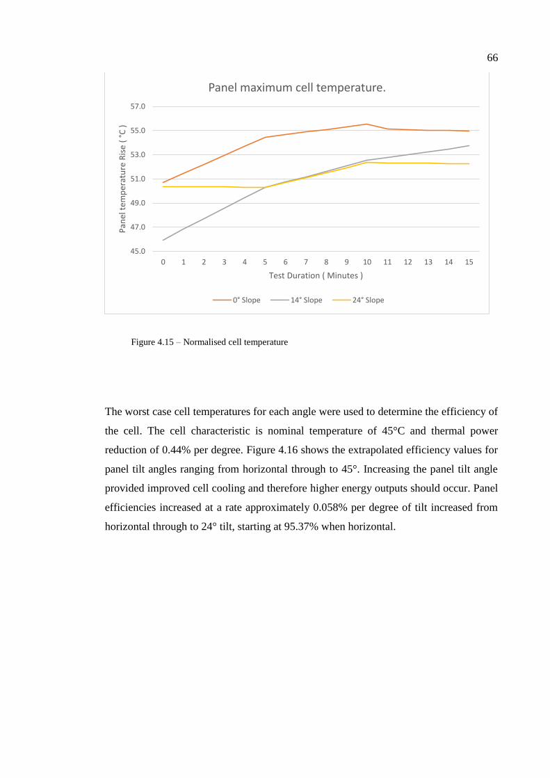
66
Figure 4.15 – Normalised cell temperature
The worst case cell temperatures for each angle were used to determine the efficiency of
the cell. The cell characteristic is nominal temperature of 45°C and thermal power
reduction of 0.44% per degree. Figure 4.16 shows the extrapolated efficiency values for
panel tilt angles ranging from horizontal through to 45°. Increasing the panel tilt angle
provided improved cell cooling and therefore higher energy outputs should occur. Panel
efficiencies increased at a rate approximately 0.058% per degree of tilt increased from
horizontal through to 24° tilt, starting at 95.37% when horizontal.
45.0
47.0
49.0
51.0
53.0
55.0
57.0
0 1 2 3 4 5 6 7 8 9 10 11 12 13 14 15
Pan
el t
emp
erat
ure
Ris
e (
°C )
Test Duration ( Minutes )
Panel maximum cell temperature.
0° Slope 14° Slope 24° Slope
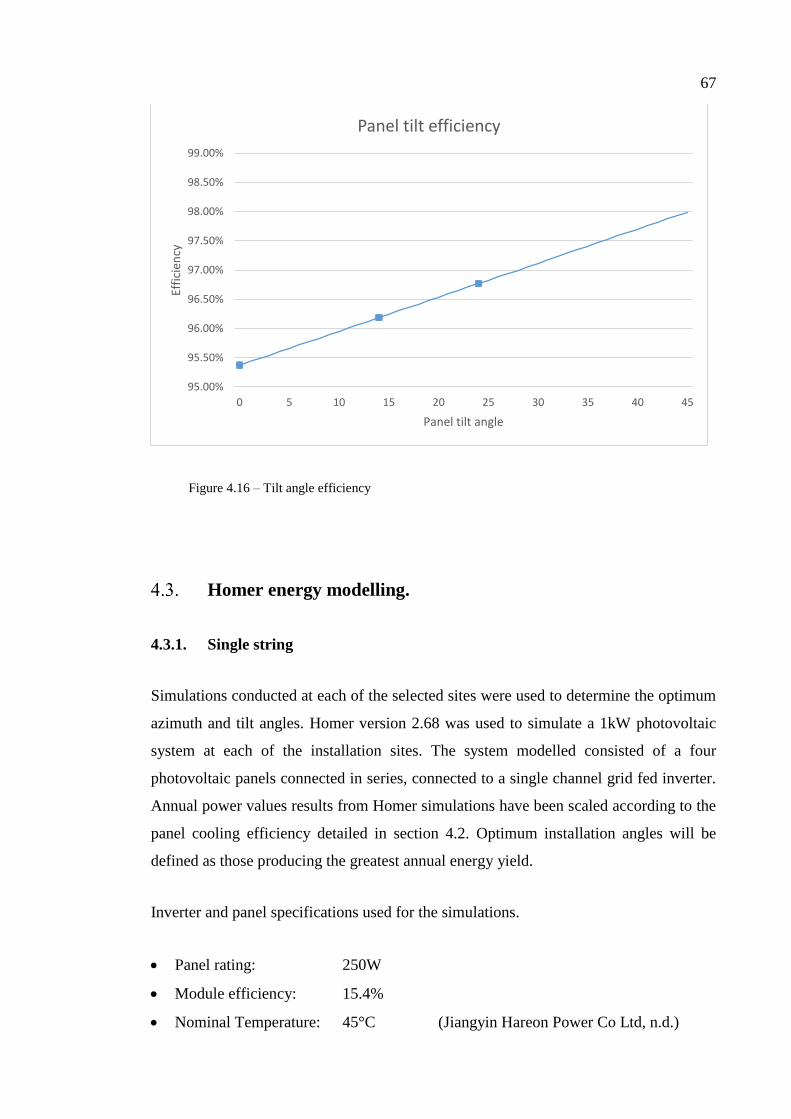
67
Figure 4.16 – Tilt angle efficiency
Homer energy modelling.
4.3.1. Single string
Simulations conducted at each of the selected sites were used to determine the optimum
azimuth and tilt angles. Homer version 2.68 was used to simulate a 1kW photovoltaic
system at each of the installation sites. The system modelled consisted of a four
photovoltaic panels connected in series, connected to a single channel grid fed inverter.
Annual power values results from Homer simulations have been scaled according to the
panel cooling efficiency detailed in section 4.2. Optimum installation angles will be
defined as those producing the greatest annual energy yield.
Inverter and panel specifications used for the simulations.
Panel rating: 250W
Module efficiency: 15.4%
Nominal Temperature: 45°C (Jiangyin Hareon Power Co Ltd, n.d.)
95.00%
95.50%
96.00%
96.50%
97.00%
97.50%
98.00%
98.50%
99.00%
0 5 10 15 20 25 30 35 40 45
Effi
cien
cy
Panel tilt angle
Panel tilt efficiency

68
No of MPPT: 1
Maximum Input Power: 1100W
Maximum efficiency: 97% (Foshan ASEP Industrial Electronics Co, Ltd,
2015)
Optimum installation angle: 15 degree resolution.
Installing solar panels facing north provides the highest annual energy yield. Figure 4.17a
shows the installation tilt angle relative to the installation azimuth for the Brooklyn Park
site. As the installation azimuth angle is varied from the north, the maximum capability
of the system is reduced. In order to maintain maximum power, the tilt angle must be
reduced for azimuth angles other than the optimum. The maximum capability of panels
installed at an azimuth 90° or more either direction from north occurs when the panels
are parallel with the surface of the earth, occurring on all of the sites modelled. Graphs
for each site can be located in appendix E.
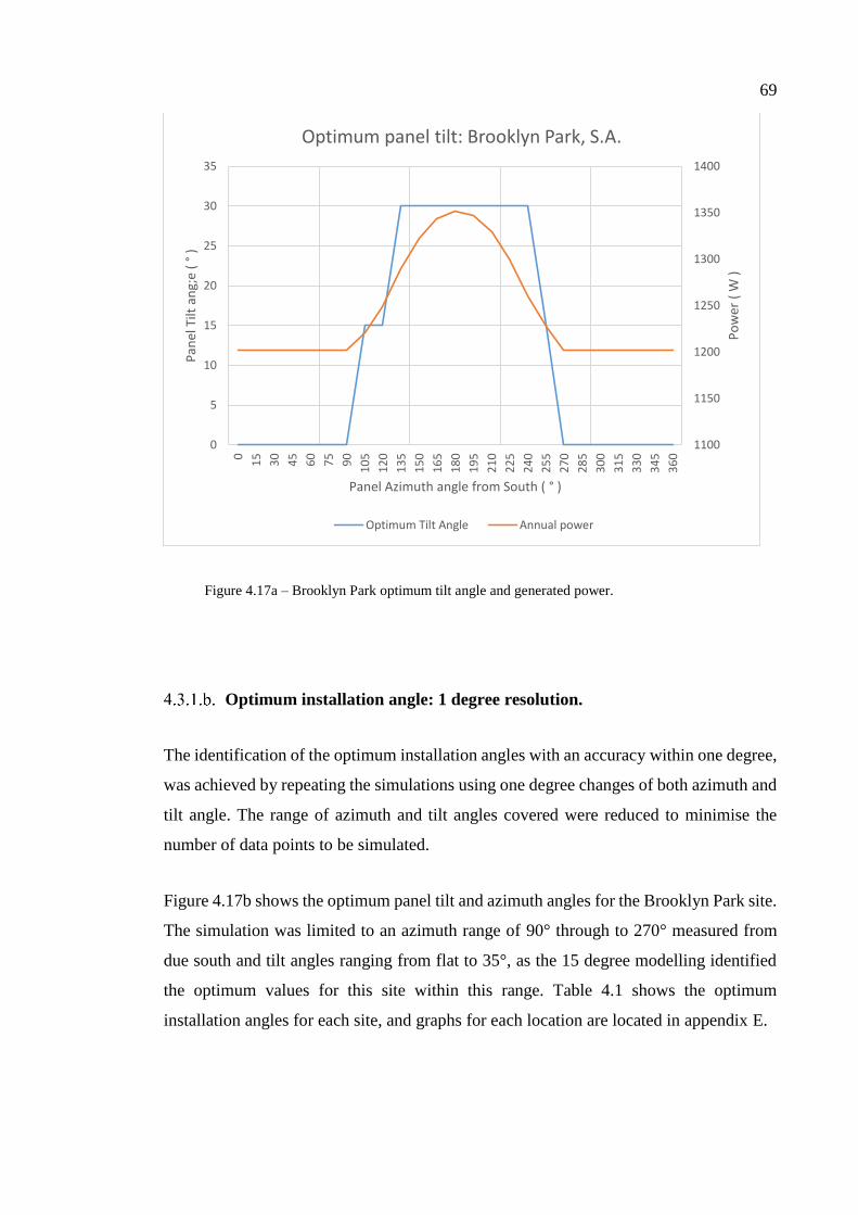
69
Figure 4.17a – Brooklyn Park optimum tilt angle and generated power.
Optimum installation angle: 1 degree resolution.
The identification of the optimum installation angles with an accuracy within one degree,
was achieved by repeating the simulations using one degree changes of both azimuth and
tilt angle. The range of azimuth and tilt angles covered were reduced to minimise the
number of data points to be simulated.
Figure 4.17b shows the optimum panel tilt and azimuth angles for the Brooklyn Park site.
The simulation was limited to an azimuth range of 90° through to 270° measured from
due south and tilt angles ranging from flat to 35°, as the 15 degree modelling identified
the optimum values for this site within this range. Table 4.1 shows the optimum
installation angles for each site, and graphs for each location are located in appendix E.
1100
1150
1200
1250
1300
1350
1400
0
5
10
15
20
25
30
35
0
15
30
45
60
75
90
10
5
12
0
13
5
15
0
16
5
18
0
19
5
21
0
22
5
24
0
25
5
27
0
28
5
30
0
31
5
33
0
34
5
36
0
Po
wer
( W
)
Pan
el T
ilt a
ng;
e (
°)
Panel Azimuth angle from South ( ° )
Optimum panel tilt: Brooklyn Park, S.A.
Optimum Tilt Angle Annual power
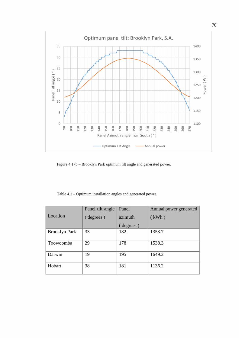
70
Figure 4.17b – Brooklyn Park optimum tilt angle and generated power.
Table 4.1 – Optimum installation angles and generated power.
Location
Panel tilt angle
( degrees )
Panel
azimuth
( degrees )
Annual power generated
( kWh )
Brooklyn Park 33 182 1353.7
Toowoomba 29 178 1538.3
Darwin 19 195 1649.2
Hobart 38 181 1136.2
1100
1150
1200
1250
1300
1350
1400
0
5
10
15
20
25
30
35
90
10
0
11
0
12
0
13
0
14
0
15
0
16
0
17
0
18
0
19
0
20
0
21
0
22
0
23
0
24
0
25
0
26
0
27
0
Po
wer
( W
)
Pan
el T
ilt a
ng;
e (
°)
Panel Azimuth angle from South ( ° )
Optimum panel tilt: Brooklyn Park, S.A.
Optimum Tilt Angle Annual power

71
Site position effect on optimum installation angle.
The effect of site location was investigated by repeating the simulation for each of the
four sites to the north, south, east and west. Temperature data remained unchanged,
however the solar radiation was updated to reflect the modified location.
The installation angles providing the greatest annual energy yield were affected by a
change to the geographic location of the site, with results shown in table 4.2. Minimal
effect was observed on the optimum azimuth angle with changes to the latitude, similarly
the effect of the tilt angle was minor for changes to the site longitude. The change in
optimum azimuth angle for Darwin was vastly different to the remaining sites, therefore
omitted from the average difference. This may be due to the close proximity to the equator
and will need further investigation.
Changes in site latitude presented a noticeable effect to the tilt angle, while changes in
the longitude showed similar results for changes to the longitude. Simulations indicated
a change to the optimum tilt angle of 0.85° per degree of latitude, while results for the
azimuth indicated a change of 0.9° per degree of longitude. With the other angle set to
the optimum position. These results were averaged across all four simulated sites.
Increasing the site latitude required an increased angle of tilt to maintain optimum power
generation while moving the site to an increased longitude (east) required a decrease of
the installation azimuth.
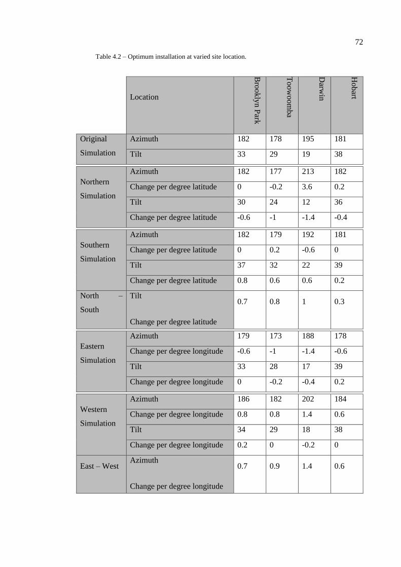
72
Table 4.2 – Optimum installation at varied site location.
Location
Bro
okly
n P
ark
Toow
oom
ba
Darw
in
Hobart
Original
Simulation
Azimuth 182 178 195 181
Tilt 33 29 19 38
Northern
Simulation
Azimuth 182 177 213 182
Change per degree latitude 0 -0.2 3.6 0.2
Tilt 30 24 12 36
Change per degree latitude -0.6 -1 -1.4 -0.4
Southern
Simulation
Azimuth 182 179 192 181
Change per degree latitude 0 0.2 -0.6 0
Tilt 37 32 22 39
Change per degree latitude 0.8 0.6 0.6 0.2
North –
South
Tilt
Change per degree latitude
0.7 0.8 1 0.3
Eastern
Simulation
Azimuth 179 173 188 178
Change per degree longitude -0.6 -1 -1.4 -0.6
Tilt 33 28 17 39
Change per degree longitude 0 -0.2 -0.4 0.2
Western
Simulation
Azimuth 186 182 202 184
Change per degree longitude 0.8 0.8 1.4 0.6
Tilt 34 29 18 38
Change per degree longitude 0.2 0 -0.2 0
East – West Azimuth
Change per degree longitude
0.7 0.9 1.4 0.6
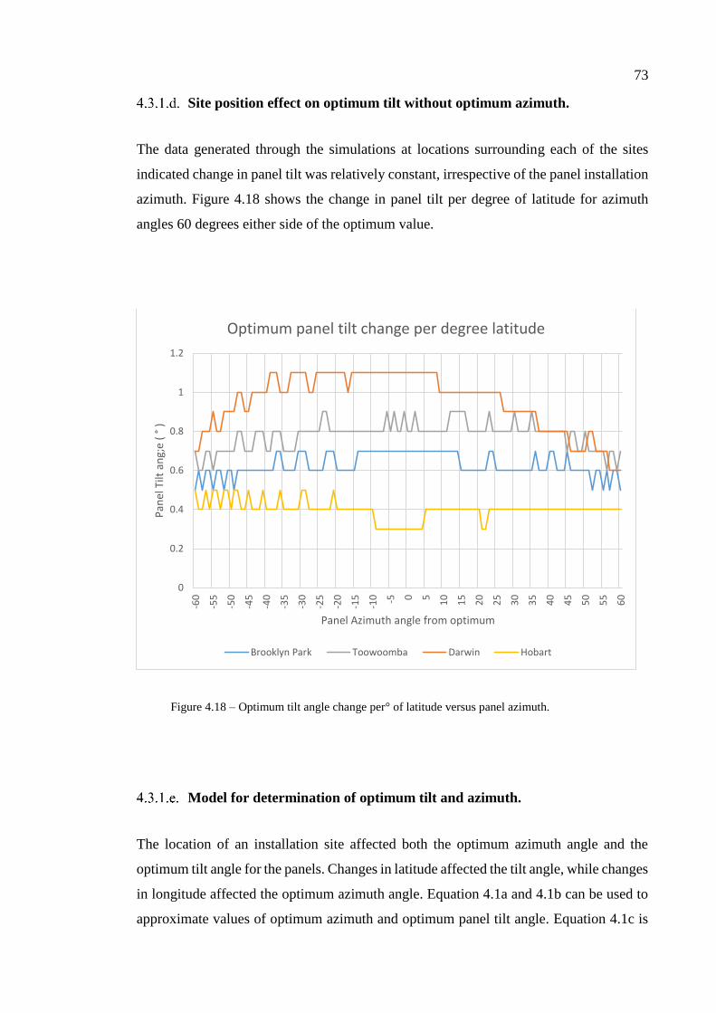
73
Site position effect on optimum tilt without optimum azimuth.
The data generated through the simulations at locations surrounding each of the sites
indicated change in panel tilt was relatively constant, irrespective of the panel installation
azimuth. Figure 4.18 shows the change in panel tilt per degree of latitude for azimuth
angles 60 degrees either side of the optimum value.
Figure 4.18 – Optimum tilt angle change per° of latitude versus panel azimuth.
Model for determination of optimum tilt and azimuth.
The location of an installation site affected both the optimum azimuth angle and the
optimum tilt angle for the panels. Changes in latitude affected the tilt angle, while changes
in longitude affected the optimum azimuth angle. Equation 4.1a and 4.1b can be used to
approximate values of optimum azimuth and optimum panel tilt angle. Equation 4.1c is
0
0.2
0.4
0.6
0.8
1
1.2
-60
-55
-50
-45
-40
-35
-30
-25
-20
-15
-10 -5 0 5
10
15
20
25
30
35
40
45
50
55
60
Pan
el T
ilt a
ng;
e (
°)
Panel Azimuth angle from optimum
Optimum panel tilt change per degree latitude
Brooklyn Park Toowoomba Darwin Hobart
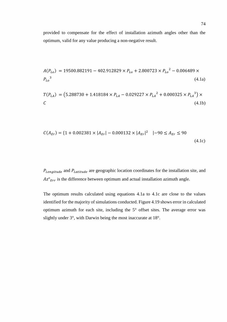
74
provided to compensate for the effect of installation azimuth angles other than the
optimum, valid for any value producing a non-negative result.
𝐴(𝑃𝐿𝑜) = 19500.882191 − 402.912829 × 𝑃𝐿𝑜 + 2.800723 × 𝑃𝐿𝑜2 − 0.006489 ×
𝑃𝐿𝑜3 (4.1a)
𝑇(𝑃𝐿𝐴) = (5.288730 + 1.418184 × 𝑃𝐿𝐴 − 0.029227 × 𝑃𝐿𝐴2 + 0.000325 × 𝑃𝐿𝐴
3) ×
𝐶 (4.1b)
𝐶(𝐴𝐸𝑟) = {1 + 0.002381 × |𝐴𝐸𝑟| − 0.000132 × |𝐴𝐸𝑟|2 |−90 ≤ 𝐴𝐸𝑟 ≤ 90
(4.1c)
𝑃𝐿𝑜𝑛𝑔𝑖𝑡𝑢𝑑𝑒 and 𝑃𝐿𝑎𝑡𝑖𝑡𝑢𝑑𝑒 are geographic location coordinates for the installation site, and
𝐴𝑧°𝐸𝑟𝑟 is the difference between optimum and actual installation azimuth angle.
The optimum results calculated using equations 4.1a to 4.1c are close to the values
identified for the majority of simulations conducted. Figure 4.19 shows error in calculated
optimum azimuth for each site, including the 5° offset sites. The average error was
slightly under 3°, with Darwin being the most inaccurate at 18°.
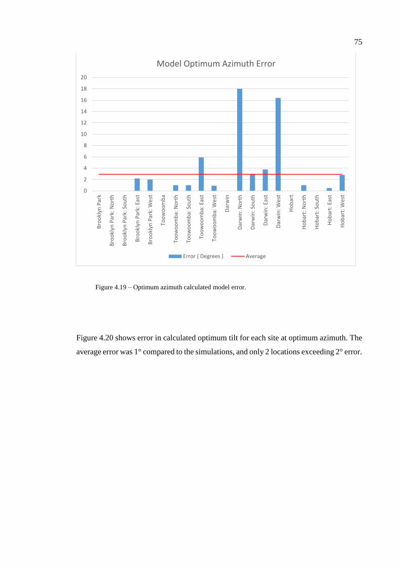
75
Figure 4.19 – Optimum azimuth calculated model error.
Figure 4.20 shows error in calculated optimum tilt for each site at optimum azimuth. The
average error was 1° compared to the simulations, and only 2 locations exceeding 2° error.
0
2
4
6
8
10
12
14
16
18
20
Bro
okl
yn P
ark
Bro
okl
yn P
ark:
No
rth
Bro
okl
yn P
ark:
So
uth
Bro
okl
yn P
ark:
Eas
t
Bro
okl
yn P
ark:
We
st
Too
wo
om
ba
Too
wo
om
ba:
No
rth
Too
wo
om
ba:
So
uth
Too
wo
om
ba:
Eas
t
Too
wo
om
ba:
We
st
Dar
win
Dar
win
: N
ort
h
Dar
win
: So
uth
Dar
win
: Ea
st
Dar
win
: W
est
Ho
bar
t
Ho
bar
t: N
ort
h
Ho
bar
t: S
ou
th
Ho
bar
t: E
ast
Ho
bar
t: W
est
Model Optimum Azimuth Error
Error ( Degrees ) Average
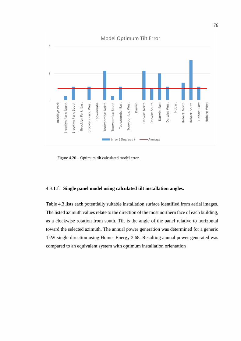
76
Figure 4.20 – Optimum tilt calculated model error.
Single panel model using calculated tilt installation angles.
Table 4.3 lists each potentially suitable installation surface identified from aerial images.
The listed azimuth values relate to the direction of the most northern face of each building,
as a clockwise rotation from south. Tilt is the angle of the panel relative to horizontal
toward the selected azimuth. The annual power generation was determined for a generic
1kW single direction using Homer Energy 2.68. Resulting annual power generated was
compared to an equivalent system with optimum installation orientation
0
2
4
Bro
okl
yn P
ark
Bro
okl
yn P
ark:
No
rth
Bro
okl
yn P
ark:
So
uth
Bro
okl
yn P
ark:
Eas
t
Bro
okl
yn P
ark:
We
st
Too
wo
om
ba
Too
wo
om
ba:
No
rth
Too
wo
om
ba:
So
uth
Too
wo
om
ba:
Eas
t
Too
wo
om
ba:
We
st
Dar
win
Dar
win
: N
ort
h
Dar
win
: So
uth
Dar
win
: Ea
st
Dar
win
: W
est
Ho
bar
t
Ho
bar
t: N
ort
h
Ho
bar
t: S
ou
th
Ho
bar
t: E
ast
Ho
bar
t: W
est
Model Optimum Tilt Error
Error ( Degrees ) Average
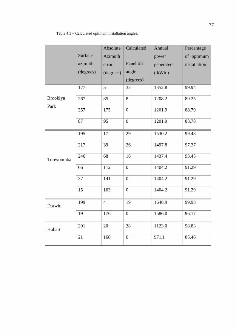
77
Table 4.3 – Calculated optimum installation angles.
Surface
azimuth
(degrees)
Absolute
Azimuth
error
(degrees)
Calculated
Panel tilt
angle
(degrees)
Annual
power
generated
( kWh )
Percentage
of optimum
installation
Brooklyn
Park
177 5 33 1352.8 99.94
267 85 8 1208.2 89.25
357 175 0 1201.9 88.79
87 95 0 1201.9 88.78
Toowoomba
195 17 29 1530.2 99.48
217 39 26 1497.8 97.37
246 68 16 1437.4 93.45
66 112 0 1404.2 91.29
37 141 0 1404.2 91.29
15 163 0 1404.2 91.29
Darwin
199 4 19 1648.9 99.98
19 176 0 1586.0 96.17
Hobart
201 20 38 1123.0 98.83
21 160 0 971.1 85.46
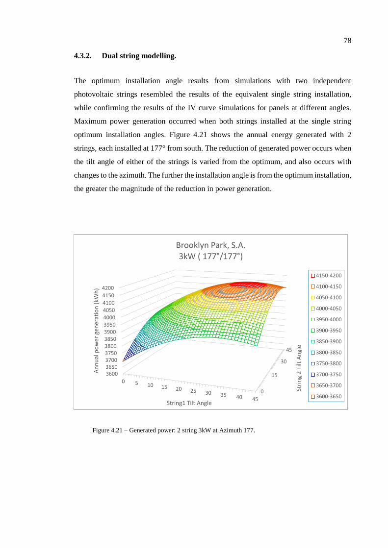
78
4.3.2. Dual string modelling.
The optimum installation angle results from simulations with two independent
photovoltaic strings resembled the results of the equivalent single string installation,
while confirming the results of the IV curve simulations for panels at different angles.
Maximum power generation occurred when both strings installed at the single string
optimum installation angles. Figure 4.21 shows the annual energy generated with 2
strings, each installed at 177° from south. The reduction of generated power occurs when
the tilt angle of either of the strings is varied from the optimum, and also occurs with
changes to the azimuth. The further the installation angle is from the optimum installation,
the greater the magnitude of the reduction in power generation.
Figure 4.21 – Generated power: 2 string 3kW at Azimuth 177.
0
15
30
45
3600365037003750380038503900395040004050
4100
4150
4200
0 5 10 15 20 25 30 35 40 45
Stri
ng
2 T
ilt A
ngl
e
An
nu
al p
ow
er g
ener
atio
n (
kWh
)
String1 Tilt Angle
Brooklyn Park, S.A.3kW ( 177°/177°)
4150-4200
4100-4150
4050-4100
4000-4050
3950-4000
3900-3950
3850-3900
3800-3850
3750-3800
3700-3750
3650-3700
3600-3650

79
5. Conclusion
There are many factors identified throughout this dissertation which affect the volume of
energy generated by a photovoltaic installation. The design of such systems can be used
to accommodate some of these factors including but not limited to, panel angle, panel
efficiency and inverter configuration. Factors such as temperature and solar irradiance are
beyond our control.
The connection of a number of solar panels together will lead to an increase in the system
output. Differences from one panel to the next combined with unequal energy input and
variations in installation conditions. The effect parallel and series connected panels
installed at two separate angles leads to energy losses within the system, and generally
increases as the difference in angle is increased. Under most conditions, the magnitude of
these losses remained constant while the difference in angle was less than 10°.
Panels which have been installed within 15 degrees from north should generate more
energy over a year than other azimuth ranges. Therefore installation should be prioritised
to the roof surface facing nearest to north, and the tilt angle should be set relative to the
actual installation azimuth. Equations 4.1a, 4.1b and 4.1c can assist in the determination
of the optimum angles for installation.
Wherever possible, the installation of solar panels in locations which are subjected to a
large amount of shading should be avoided. Where there is no possibility of installing the
system in a location completely free of shade, the D.C. connection between must not be
connected in parallel as this will lead to substantial energy losses.
The selection of the inverter is an equally important factor in the design of a solar energy
system. The system designer must take care to ensure the maximum voltage generated
within each string does not exceed the maximum input of the inverter, at the same time
maximising the time where the string voltage will exceed the minimum voltage required
to drive the circuitry of the inverter. The maximum power capable of being delivered to
the input of the inverter should remain within a range 30 - 100% of the rating of the input.
Operating outside of this range will lead to a decreased efficiency of the system Inverters
with dual maximum power point tracking provided the lowest efficiency losses for two
80
string systems. The use of two inverters, or a single channel power point tracking inverters
were able to demonstrate similar efficiency values, generally only when all panels were
installed on common orientation.
Further work.
Information identified throughout the course of this research has provided opportunity for
further work into the optimisation of solar power systems.
Modelling which was conducted within Matlab was limited to two separate panels
connected in either series or parallel. Shading was modelled by reducing the panel output
relative to the shaded area. The model could be revised to include the effect of partial
shading over the panel. Modelling the IV curve of each cell separately using a common
voltage vector could assist in the analysis of more complex shading patterns, and the
effect of a combination of connection methods.
The intention of the energy optimisation model was to maximise the power generated
using photovoltaic solar power systems, although this approach may not provide
maximum benefit for all circumstances. The model could be revised to include a profile
of electrical demand to identify, allowing customisation of the model to a consumers
requirements.
The geographic locations used for the optimisation simulations covered a wide range of
latitudes, ranging from the far north through to the south. The locations were limited in
longitude covering a range from central Australia through to the east coast. The model
could be extended to include locations across to the west coast.
81
6. References
Ahfock, A 2011, ELE3805 Power electronics principles and communications: Study
book 1, University of Southern Queensland, Toowoomba.
Bellini, A, Bifaretti, S, Iacovone, V, Cornaro, C n.d. 'Simplified Model of a Photovoltaic
Module’, viewed 2 May 2015,
<http://www.google.com.au/url?sa=t&rct=j&q=&esrc=s&source=web&cd=13&cad=rja
&uact=8&ved=0CGEQFjAM&url=http%3A%2F%2Fwww.researchgate.net%2Fprofile
%2FCristina_Cornaro%2Fpublication%2F224605112_Simplified_model_of_a_photovo
ltaic_module%2Flinks%2F0c960527a618b46d97000000.pdf&ei=yq9EVYzjJKHGmQ
X_-IG4Ag&usg=AFQjCNGwdKwEr3DKEbDpo_2B-
ryaRMoPYg&bvm=bv.92291466,d.dGY>
Commonwealth of Australia 2015, 'Climate Data Online', Bureau of Meteorology,
viewed 18 March 2015, <http://www.bom.gov.au/climate/data/>
Cornwall, C, Horiuchi, A & Lehman, C, 2015. 'Solar Position Calculator', viewed 29
September 2015, <http://www.esrl.noaa.gov/gmd/grad/solcalc/azel.html>
Encyclopædia Britannica, Inc. 2015a, Brewsters Law, viewed 8 June 2015,
<http://www.britannica.com/EBchecked/topic/79080/Brewsters-law>
Encyclopædia Britannica, Inc. 2015b, Refractive index, viewed 8 June 2015,
<http://www.britannica.com/EBchecked/topic/495677/refractive-index>
ENG4111 Research project part 1: Project reference book 2014 , University of Southern
Queensland, Toowoomba.
European Agency for Safety and Health at Work, n.d. HAZARD IDENTIFICATION
CHECKLIST: OSH RISKS ASSOCIATED WITH SMALL-SCALE SOLAR ENERGY
APPLICATIONS, viewed 20 May 2015,
<https://www.google.com.au/url?sa=t&rct=j&q=&esrc=s&frm=1&source=web&cd=1
&cad=rja&uact=8&ved=0CDkQFjAA&url=https%3A%2F%2Fosha.europa.eu%2Fen%
82
2Fpublications%2Fe-facts%2Fe-fact-69-hazard-identification-checklist-osh-risks-
associated-with-small-scale-solar-energy-
applications&ei=a3ZcVc6hB4bNmwWXpYDoAg&usg=AFQjCNEML9PgSjaT3bGcv
w2S9gVIzfeNwQ&bvm=bv.93756505,d.dGY>.
Folsom Labs, 2014, Inverter Modelling, viewed 25 September 2015,
<https://www.folsomlabs.com/modeling/system/inverter>
Foshan ASEP Industrial Electronics Co, Ltd. 2014, Single Channel Grid-Tie Inverter,
viewed 15 May 2015, <http://www.asepups.com/single-channel-grid-tie-inverter1.html>
Google, 2015, Google Maps, viewed May 2015, <https://www.google.com.au/maps>
Green Rhino Energy Ltd. 2013, Solar power: Radiation, viewed 25 April 2015,
<http://www.greenrhinoenergy.com/solar/radiation/characteristics.php>
Homer Energy 2015, The HOMER® Microgrid Software, viewed 21 October 2015,
<http://www.homerenergy.com/software.html>
Honsberg, C & Bowden, S 2013a, Air Mass, viewed 29 March 2015,
<http://pveducation.org/pvcdrom/properties-of-sunlight/air-mass>
Honsberg, C & Bowden, S 2013b, Anti-Reflection Coatings, viewed 29 March 2015,
<http://pveducation.org/pvcdrom/design/anti-reflection-coatings>
Honsberg, C & Bowden, S 2013c, Bypass Diodes, viewed 29 March 2015,
<http://pveducation.org/pvcdrom/modules/bypass-diodes>
Honsberg, C & Bowden, S 2013d, Characteristic Resistance, viewed 29 March 2015,
<http://pveducation.org/pvcdrom/solar-cell-operation/charecteristic-resistance>
Honsberg, C & Bowden, S 2013e, Effect of parasitic Resistances, viewed 29 March 2015,
<http://pveducation.org/pvcdrom/solar-cell-operation/effect-of-parasitic-resistances>
83
Honsberg, C & Bowden, S 2013f, Effect of Temperature, viewed 29 March 2015,
<http://pveducation.org/pvcdrom/solar-cell-operation/effect-of-temperature>
Honsberg, C & Bowden, S 2013g, Efficiency, viewed 29 March 2015,
<http://pveducation.org/pvcdrom/solar-cell-operation/efficiency>
Honsberg, C & Bowden, S 2013h, Energy of Photon, viewed 29 March 2015,
<http://pveducation.org/pvcdrom/properties-of-sunlight/energy-of-photon>
Honsberg, C & Bowden, S 2013i, Heat Generation in PV Modules, viewed 29 March
2015, <http://pveducation.org/pvcdrom/modules/heat-generation-in-pv-modules>
Honsberg, C & Bowden, S 2013j, Hot Spot Heating, viewed 29 March 2015,
<http://pveducation.org/pvcdrom/modules/hot-spot-heating>
Honsberg, C & Bowden, S 2013k, Mismatch Effects, viewed 29 March 2015,
<http://pveducation.org/pvcdrom/modules/mismatch-effects>
Honsberg, C & Bowden, S 2013m, Optical Losses, viewed 29 March 2015,
<http://pveducation.org/pvcdrom/design/optical-losses>
Honsberg, C & Bowden, S 2013n, Photon Flux, viewed 29 March 2015,
<http://pveducation.org/pvcdrom/properties-of-sunlight/photon-flux>
Honsberg, C & Bowden, S 2013o, Properties of Light, viewed 29 March 2015,
<http://pveducation.org/pvcdrom/properties-of-sunlight/properties-of-light>
Honsberg, C & Bowden, S 2013p, Radiant Power Density, viewed 29 March 2015,
<http://pveducation.org/pvcdrom/properties-of-sunlight/radiant-power-density>
Honsberg, C & Bowden, S 2013q, Series Resistance, viewed 29 March 2015,
<http://pveducation.org/pvcdrom/solar-cell-operation/series-resistance>
Honsberg, C & Bowden, S 2013r, Shunt Resistance, viewed 29 March 2015,
<http://pveducation.org/pvcdrom/solar-cell-operation/shunt-resistance>

84
Honsberg, C & Bowden, S 2013s, Solar Radiation on a Tilted Surface, viewed 29 March
2015, <http://pveducation.org/pvcdrom/properties-of-sunlight/solar-radiation-on-tilted-
surface>
Honsberg, C & Bowden, S 2013t, Surface Texturing, viewed 29 March 2015,
<http://pveducation.org/pvcdrom/design/surface-texturing>
Honsberg, C & Bowden, S 2013u, Heat Loss in PV Modules, viewed 29 March 2015,
<http://pveducation.org/pvcdrom/modules/heat-loss-in-pv-modules>
Howell, J, Menguc, P & Siegel, R 2010, 'Thermal Radiation Heat Transfer', CRC Press.
Jiangyin Hareon Power Co Ltd, n.d, Solar Module.
Jordan, D & Kurtz, S , 'Photovoltaic Degradation Rates — An Analytical Review',
Photovoltaics: Research and Applications, viewed 18 March 2015,
<http://www.nrel.gov/docs/fy12osti/51664.pdf>
Larson, R & Falvo, D 2009, Elementary linear algebra, Horton Mifflin Harcourt
Publishing Company, Boston.
Migan, G, 2013 'Study of the operating temperature of a PV module',
<http://www.google.com.au/url?sa=t&rct=j&q=&esrc=s&frm=1&source=web&cd=14
&cad=rja&uact=8&ved=0CCsQFjADOApqFQoTCK6joqnZkcgCFYgolAod6aEEpA&
url=http%3A%2F%2Fwww.ht.energy.lth.se%2Ffileadmin%2Fht%2FKurser%2FMVK1
60%2F2012%2FGail-
Angee_Migan.pdf&usg=AFQjCNFsSU9gLkEQiPY1kRGXcdphRu5Csg&bvm=bv.103
627116,d.dGo>
MPPT Solar n.d a, Connecting solar panels in parallel, viewed 8 June 2015,
<http://www.mpptsolar.com/en/solar-panels-in-parallel.html>
MPPT Solar n.d b, Connecting solar panels in series, viewed 8 June 2015,
<http://www.mpptsolar.com/en/solar-panels-in-series.html>

85
National Instruments, 2009a 'Part I – Photovoltaic Cell Overview', National Instruments,
Austin, Texas, USA, viewed 29 March 2015, <http://www.ni.com/white-paper/7229/en/>
National Instruments, 2009b 'Part II – Photovoltaic Cell I-V Characterization Theory and
LabVIEW Analysis Code', National Instruments, Austin, Texas, USA, viewed 29 March
2015, <http://www.ni.com/white-paper/7230/en/>
National Instruments, 2009c 'Maximum Power Point Tracking', National Instruments,
Austin, Texas, USA, viewed 29 March 2015, <http://www.ni.com/white-paper/8106/en/>
Palm, W 2009, Introduction to MATLAB for engineers, McGraw Hill, New York.
Pandit, PK & Chaurasia, PBL 2014 'Experimental Study of Shading Effect on PV Module
and Improvement in Power Using Diode on Series & Parallel PV Module', International
Journal of Science and Research (IJSR), vol. 3, issue. 6, viewed 8 April 2015,
<http://ijsr.net/archive/v3i6/MDIwMTQ1MjE%3D.pdf>
Perlin, J n.d, A History of Photovoltaic, viewed 12 March 2015,
<http://www.usc.edu/org/edisonchallenge/2008/ws1/A%20History%20of%20Photovolt
aics.pdf>
Renew Economy, 2015, Australia reaches 4GW of rooftop solar PV, viewed 25 July
2015, <http://reneweconomy.com.au/2014/australia-reaches-4gw-rooftop-solar-pv-
44719>
Rosenblatt, L 2015 'A GRID TIE INVERTER FOR SOLAR SYSTEMS', viewed 19 April
2015, <http://solar.smps.us/grid-tie-inverter-schematic.html>
Safe work Australia, 2011 'HOW TO MANAGE WORK HEALTH AND SAFETY RISKS'
Code of Practice.
Sargosis Solar & Electric 2014a, Calculating the IV and PV curves for a Solar Module,
viewed 7 April 2015, <http://sargosis.com/articles/science/how-pv-modules-
work/calculating-the-iv-and-pv-curves-for-a-solar-module/>
86
Sargosis Solar & Electric 2014b, How Shade Affects a Solar Array, viewed 20 June 2015,
<http://sargosis.com/articles/science/how-shade-affects-a-solar-array/>
Solar edge 2010, Technical Note Bypass Diode Effects in Shaded Conditions, viewed 20
June 2015, <http://resources.solmetric.com/get/Guide%20to%20Interpreting%20I-
V%20Curves.pdf>
Tayyan, Dr A 2006, An empirical model for Generating the IV characteristics for a
Photovoltaic system, viewed 2 May 2015,
<http://www.alaqsa.edu.ps/site_resources/aqsa_magazine/files/225.pdf>
The Florida Solar Energy Center , 2014a 'Cells, Modules and arrays', University of
Central Florida, Cocoa, Florida, USA, viewed 18 March 2015,
<http://www.fsec.ucf.edu/en/consumer/solar_electricity/basics/cells_modules_arrays.ht
m>
The Florida Solar Energy Center , 2014b, ‘How PV cells are made', University of Central
Florida, Cocoa, Florida, USA, viewed 18 March 2015,
<http://www.fsec.ucf.edu/en/consumer/solar_electricity/basics/how_cells_made.htm>
The Florida Solar Energy Center , 2014c ‘How PV cells work + more’, University of
Central Florida, Cocoa, Florida, USA, viewed 18 March 2015,
<http://www.fsec.ucf.edu/en/consumer/solar_electricity/basics/how_pv_cells_work.htm
>
Tindo Solar, 2015, Data Sheet Karra Model, Mawson Lakes.
University of Melbourne, 2004. RISK ASSESSMENT 3D Model, viewed 22 May 2015,
<http://www.google.com.au/url?sa=t&rct=j&q=&esrc=s&frm=1&source=web&cd=1&
ved=0CCQQFjAA&url=http%3A%2F%2Fwww.cab.unimelb.edu.au%2Fpdf%2Fehs3d.
doc&ei=Kg1fVdzjMYXn8AWrlIGIAw&usg=AFQjCNGEoDvOKSB2qVqDoz0xgkqg
5kHy7A&bvm=bv.93990622,d.dGc>.
Xue, Y, Chang, L, Bækhøj Kjær, S, Bordonau, J & Shimizu, T 2004 'Topologies of Single-
Phase Inverters for Small distributed power generators: An Overview', IEEE

87
TRANSACTIONS ON POWER ELECTRONICS, vol. 19, no. 5, viewed 12 February
2015,
<http://ieeexplore.ieee.org.ezproxy.usq.edu.au/stamp/stamp.jsp?tp=&arnumber=133149
2>
Yakoob, J & Abbas, E. 2014 'Experimental investigation of convection heat transferfor
laminar flow in an inclined annulus', International Journal of Mechanical Engineering
and Technology (IJMET), vol. 5, issue. 4, viewed 28 September 2015,
<http://www.iaeme.com/MasterAdmin/UploadFolder/30120140504020/301201405040
20.pdf>

Project Specification

A1
UNIVERSITY OF SOUTHERN QUEENSLAND
ENG4111 & ENG4112 Engineering research project 2015
PROJECT SPECIFICATION
Issue C,
03 April 2015
Student: Christopher KIRBY
Topic: Comparison of PV maximum power point.
Topic Author: Andreas HELWIG
Supervisor: Catherine HILLS
Enrolment: ENG4111 Semester 1, 2015
ENG4112 Semester 2, 2015
Project Aim: The final goal of this project is to provide guidelines for the installation of
photovoltaic (solar) systems within Australia. These guides will assist in maximising the
efficiency of such systems.
Programme:
Provide a basic introduction to photovoltaic (PV) panels.
Research factors affecting the efficiency of PV systems.
Research and define maximum power point tracking (MPPT).

A2
Research various inverter configurations for a 2 different direction string system.
Generate Matlab models for each configuration, accounting for the characteristics of
the inverter, panels and string design.
Based on the results obtained from the modelling, produce a set of guidelines to
optimise system output for PV systems throughout Australia.
Using Homer Energy software, model different sized PV array in differing climate
locations throughout Australia for the selected inverter configurations in order to
quantify the financial and economic benefits of system optimisation.
As time permits:
Calculate financial savings and environmental benefits from improving efficiency of
existing installations throughout Australia.
Conduct a basic feasibility into reworking existing installations to improve efficiency.
Agreed:
_Christopher J Kirby_ ( Student ) ____________________ ( Supervisor )
_04_ / _04_ / _2015_ ____ / ____ / ________

Project timeline
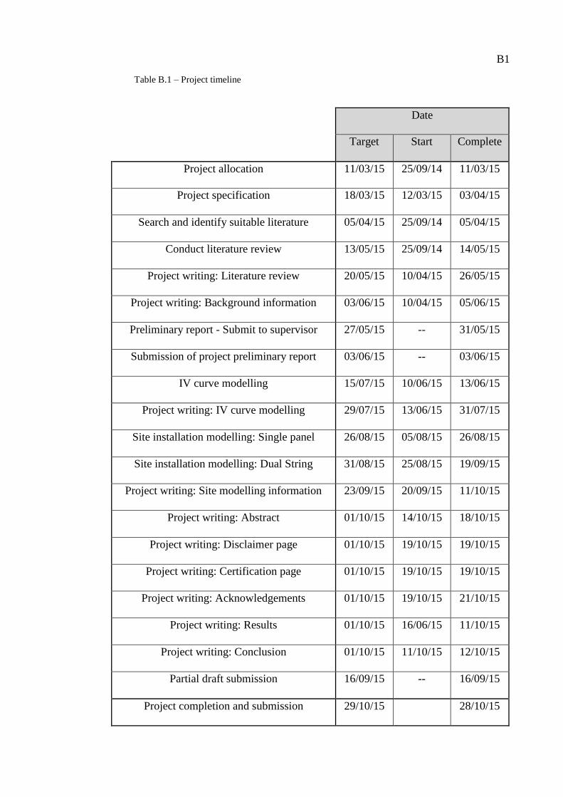
B1
Table B.1 – Project timeline
Date
Target Start Complete
Project allocation 11/03/15 25/09/14 11/03/15
Project specification 18/03/15 12/03/15 03/04/15
Search and identify suitable literature 05/04/15 25/09/14 05/04/15
Conduct literature review 13/05/15 25/09/14 14/05/15
Project writing: Literature review 20/05/15 10/04/15 26/05/15
Project writing: Background information 03/06/15 10/04/15 05/06/15
Preliminary report - Submit to supervisor 27/05/15 -- 31/05/15
Submission of project preliminary report 03/06/15 -- 03/06/15
IV curve modelling 15/07/15 10/06/15 13/06/15
Project writing: IV curve modelling 29/07/15 13/06/15 31/07/15
Site installation modelling: Single panel 26/08/15 05/08/15 26/08/15
Site installation modelling: Dual String 31/08/15 25/08/15 19/09/15
Project writing: Site modelling information 23/09/15 20/09/15 11/10/15
Project writing: Abstract 01/10/15 14/10/15 18/10/15
Project writing: Disclaimer page 01/10/15 19/10/15 19/10/15
Project writing: Certification page 01/10/15 19/10/15 19/10/15
Project writing: Acknowledgements 01/10/15 19/10/15 21/10/15
Project writing: Results 01/10/15 16/06/15 11/10/15
Project writing: Conclusion 01/10/15 11/10/15 12/10/15
Partial draft submission 16/09/15 -- 16/09/15
Project completion and submission 29/10/15 28/10/15

Derivation of formulas
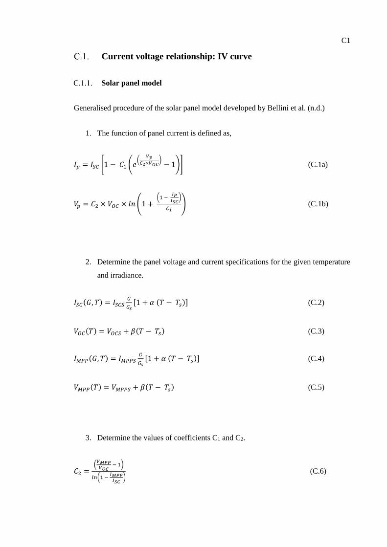
C1
Current voltage relationship: IV curve
Solar panel model
Generalised procedure of the solar panel model developed by Bellini et al. (n.d.)
1. The function of panel current is defined as,
𝐼𝑝 = 𝐼𝑆𝐶 [1 − 𝐶1 (𝑒(
𝑉𝑝
𝐶2×𝑉𝑂𝐶)
− 1)] (C.1a)
𝑉𝑝 = 𝐶2 × 𝑉𝑂𝐶 × 𝑙𝑛 (1 + (1 −
𝐼𝑃𝐼𝑆𝐶
)
𝐶1) (C.1b)
2. Determine the panel voltage and current specifications for the given temperature
and irradiance.
𝐼𝑆𝐶(𝐺, 𝑇) = 𝐼𝑆𝐶𝑆𝐺
𝐺𝑠[1 + 𝛼 (𝑇 − 𝑇𝑠)] (C.2)
𝑉𝑂𝐶(𝑇) = 𝑉𝑂𝐶𝑆 + 𝛽(𝑇 − 𝑇𝑠) (C.3)
𝐼𝑀𝑃𝑃(𝐺, 𝑇) = 𝐼𝑀𝑃𝑃𝑆𝐺
𝐺𝑠[1 + 𝛼 (𝑇 − 𝑇𝑠)] (C.4)
𝑉𝑀𝑃𝑃(𝑇) = 𝑉𝑀𝑃𝑃𝑆 + 𝛽(𝑇 − 𝑇𝑠) (C.5)
3. Determine the values of coefficients C1 and C2.
𝐶2 =(
𝑉𝑀𝑃𝑃𝑉𝑂𝐶
− 1)
𝑙𝑛(1 − 𝐼𝑀𝑃𝑃
𝐼𝑆𝐶) (C.6)
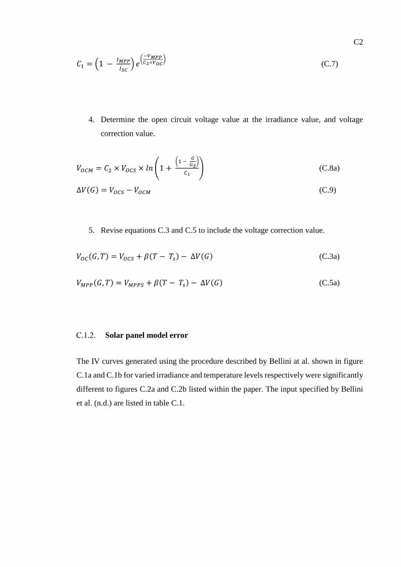
C2
𝐶1 = (1 − 𝐼𝑀𝑃𝑃
𝐼𝑆𝐶) 𝑒
(−𝑉𝑀𝑃𝑃𝐶2×𝑉𝑂𝐶
) (C.7)
4. Determine the open circuit voltage value at the irradiance value, and voltage
correction value.
𝑉𝑂𝐶𝑀 = 𝐶2 × 𝑉𝑂𝐶𝑆 × 𝑙𝑛 (1 + (1 −
𝐺
𝐺𝑆)
𝐶1) (C.8a)
∆𝑉(𝐺) = 𝑉𝑂𝐶𝑆 − 𝑉𝑂𝐶𝑀 (C.9)
5. Revise equations C.3 and C.5 to include the voltage correction value.
𝑉𝑂𝐶(𝐺, 𝑇) = 𝑉𝑂𝐶𝑆 + 𝛽(𝑇 − 𝑇𝑠) − ∆𝑉(𝐺) (C.3a)
𝑉𝑀𝑃𝑃(𝐺, 𝑇) = 𝑉𝑀𝑃𝑃𝑆 + 𝛽(𝑇 − 𝑇𝑠) − ∆𝑉(𝐺) (C.5a)
Solar panel model error
The IV curves generated using the procedure described by Bellini at al. shown in figure
C.1a and C.1b for varied irradiance and temperature levels respectively were significantly
different to figures C.2a and C.2b listed within the paper. The input specified by Bellini
et al. (n.d.) are listed in table C.1.
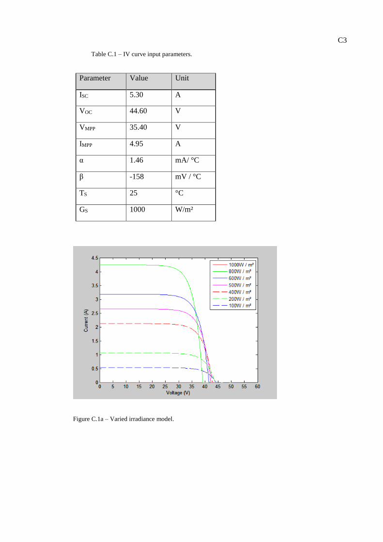
C3
Table C.1 – IV curve input parameters.
Parameter Value Unit
ISC 5.30 A
VOC 44.60 V
VMPP 35.40 V
IMPP 4.95 A
α 1.46 mA/ °C
β -158 mV / °C
TS 25 °C
GS 1000 W/m²
Figure C.1a – Varied irradiance model.
C4
Figure C.1b – Bellini et al. Varied irradiance.
Figure C.2a – Varied temperature model.
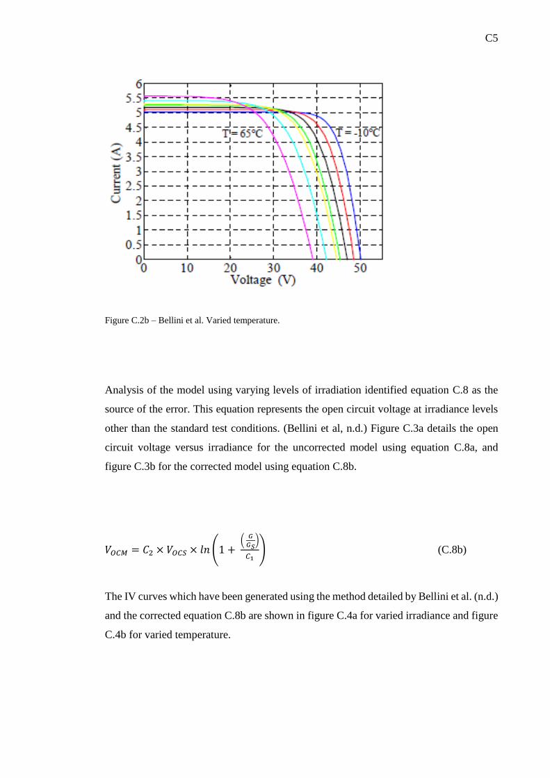
C5
Figure C.2b – Bellini et al. Varied temperature.
Analysis of the model using varying levels of irradiation identified equation C.8 as the
source of the error. This equation represents the open circuit voltage at irradiance levels
other than the standard test conditions. (Bellini et al, n.d.) Figure C.3a details the open
circuit voltage versus irradiance for the uncorrected model using equation C.8a, and
figure C.3b for the corrected model using equation C.8b.
𝑉𝑂𝐶𝑀 = 𝐶2 × 𝑉𝑂𝐶𝑆 × 𝑙𝑛 (1 + (
𝐺
𝐺𝑆)
𝐶1) (C.8b)
The IV curves which have been generated using the method detailed by Bellini et al. (n.d.)
and the corrected equation C.8b are shown in figure C.4a for varied irradiance and figure
C.4b for varied temperature.
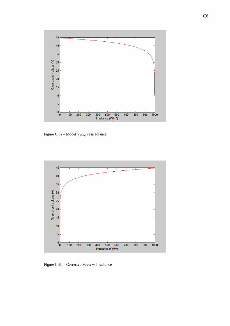
C6
Figure C.3a – Model VOCM vs irradiance.
Figure C.3b – Corrected VOCM vs irradiance
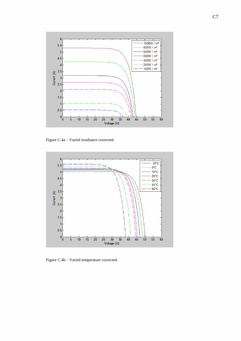
C7
Figure C.4a – Varied irradiance corrected.
Figure C.4b – Varied temperature corrected.

C8
Optimum azimuth
The function used to describe the optimum installation azimuth was defined using a polynomial curve fit based on the four locations which
were simulated in Homer.
Using the generic equation
𝑎0 + 𝑎1𝑥 + 𝑎2𝑥2 + 𝑎3𝑥3 = 𝑦0 (C.10)
Converting to augmented matrix form,
4
3
2
1
3
4
2
44
3
3
2
33
3
2
2
22
3
1
2
11
1
1
1
1
Lo
Lo
Lo
Lo
LoLoLo
LoLoLo
LoLoLo
LoLoLo
PAz
PAz
PAz
PAz
PPP
PPP
PPP
PPP
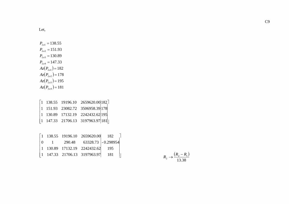
C9
Let,
181
195
178
182
33.147
89.130
93.151
55.138
4
3
2
1
4
3
2
1
Lo
Lo
Lo
Lo
Lo
Lo
Lo
Lo
PAz
PAz
PAz
PAz
P
P
P
P
181
195
178
182
3197963.9721706.1333.1471
2242432.6217132.1989.1301
3506958.3972.2308293.1511
2659620.0010.1919655.1381
181
195
0.298954-
182
3197963.9721706.1333.1471
2242432.6217132.1989.1301
63328.7348.29010
2659620.0010.1919655.1381
38.13
122
RRR
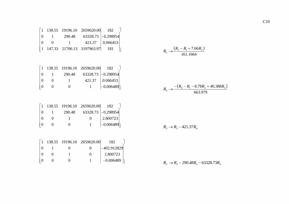
C10
181
0.066453
0.298954-
182
3197963.9721706.1333.1471
421.37100
63328.7348.29010
2659620.0010.1919655.1381
1664.161
66.7 2133
RRRR
0.006489-
0.066453
0.298954-
182
1000
421.37100
63328.7348.29010
2659620.0010.1919655.1381
979.663
388.4078.8 32144
RRRRR
0.006489-
2.800723
0.298954-
182
1000
0100
63328.7348.29010
2659620.0010.1919655.1381
433 37.421 RRR
0.006489-
2.800723
402.912829-
182
1000
0100
0010
2659620.0010.1919655.1381
4322 73.6332848.290 RRRR
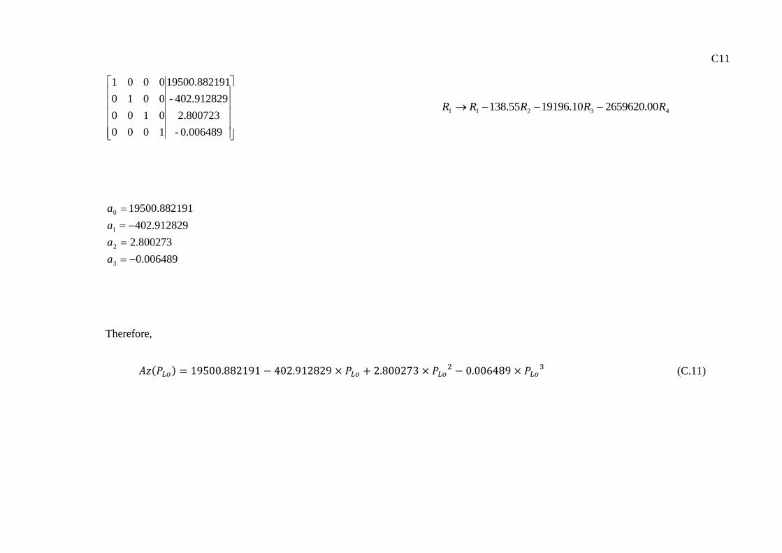
C11
0.006489-
2.800723
402.912829-
9119500.8821
1000
0100
0010
0001
43211 00.265962010.1919655.138 RRRRR
006489.0
800273.2
912829.402
882191.19500
3
2
1
0
a
a
a
a
Therefore,
𝐴𝑧(𝑃𝐿𝑜) = 19500.882191 − 402.912829 × 𝑃𝐿𝑜 + 2.800273 × 𝑃𝐿𝑜2 − 0.006489 × 𝑃𝐿𝑜
3 (C.11)

C12
Optimum tilt
The function used to describe the optimum installation tilt was defined using a polynomial curve fit based on the four locations which were
simulated in Homer. The variable C is included as a tilt angle reduction factor for installation at non optimum azimuth.
Using the generic equation
𝑎0 + 𝑎1𝑥 + 𝑎2𝑥2 + 𝑎3𝑥3 = 𝑦0 (C.10)
Converting to augmented matrix form,
4
3
2
1
3
4
2
44
3
3
2
33
3
2
2
22
3
1
2
11
1
1
1
1
LA
LA
LA
LA
LALALA
LALALA
LALALA
LALALA
PTi
PTi
PTi
PTi
PPP
PPP
PPP
PPP
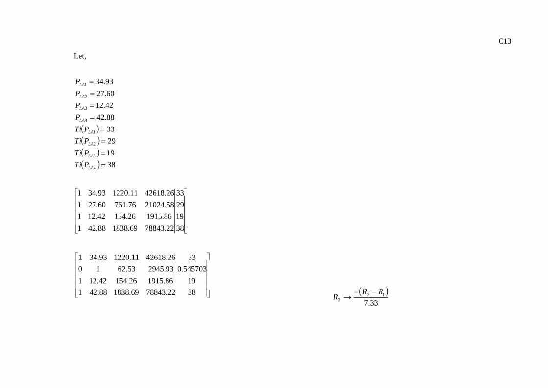
C13
Let,
38
19
29
33
88.42
42.12
60.27
93.34
4
3
2
1
4
3
2
1
LA
LA
LA
LA
LA
LA
LA
LA
PTi
PTi
PTi
PTi
P
P
P
P
38
19
29
33
22.7884369.183888.421
86.191526.15442.121
58.2102476.76160.271
26.4261811.122093.341
38
19
545703.0
33
22.7884369.183888.421
86.191526.15442.121
93.294553.6210
26.4261811.122093.341
33.7
122
RRR
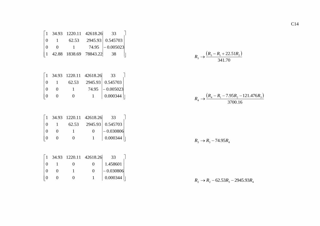
C14
38
005023.0
545703.0
33
22.7884369.183888.421
95.74100
93.294553.6210
26.4261811.122093.341
70.341
51.22 2133
RRRR
000344.0
005023.0
545703.0
33
1000
95.74100
93.294553.6210
26.4261811.122093.341
16.3700
476.12195.7 32144
RRRRR
000344.0
030806.0
545703.0
33
1000
0100
93.294553.6210
26.4261811.122093.341
433 95.74 RRR
000344.0
030806.0
458601.1
33
1000
0100
0010
26.4261811.122093.341
4322 93.294553.62 RRRR
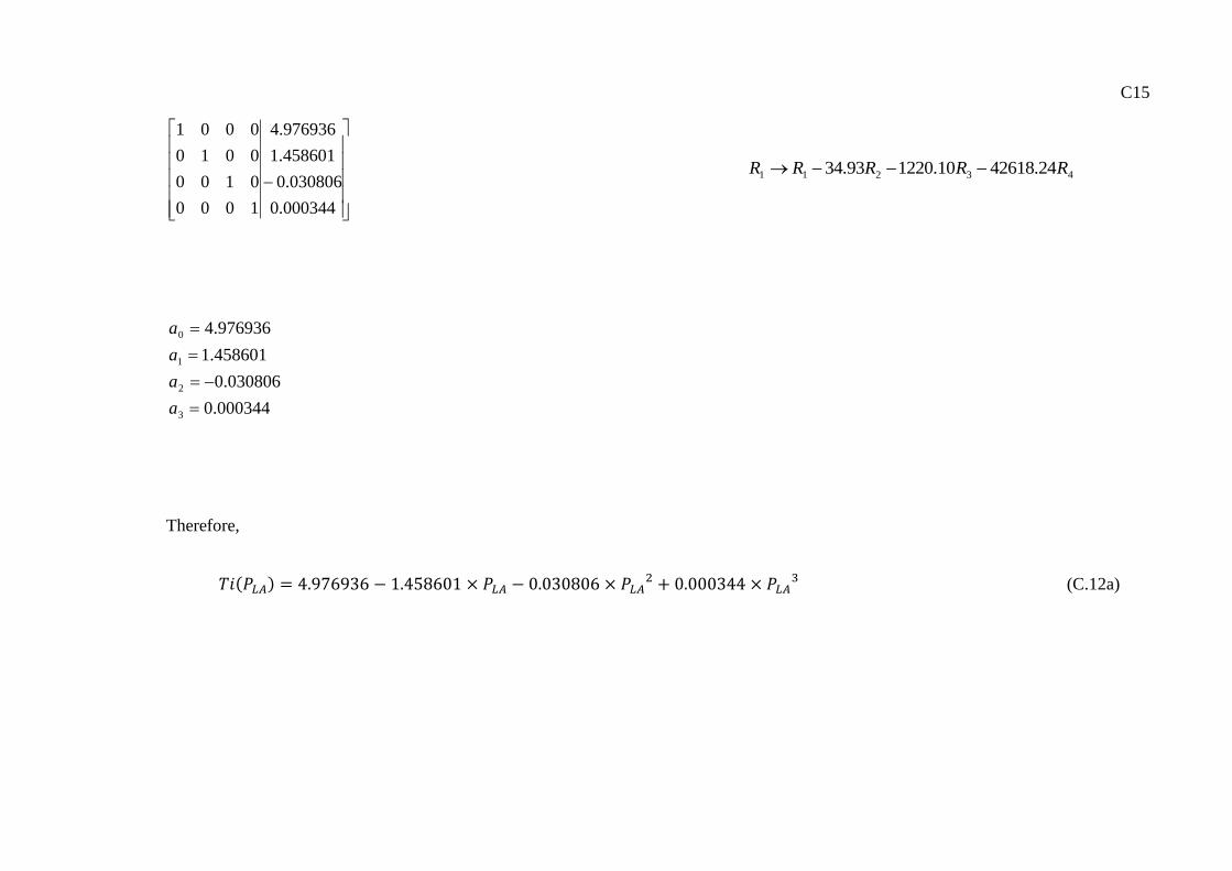
C15
000344.0
030806.0
458601.1
976936.4
1000
0100
0010
0001
43211 24.4261810.122093.34 RRRRR
000344.0
030806.0
458601.1
976936.4
3
2
1
0
a
a
a
a
Therefore,
𝑇𝑖(𝑃𝐿𝐴) = 4.976936 − 1.458601 × 𝑃𝐿𝐴 − 0.030806 × 𝑃𝐿𝐴2 + 0.000344 × 𝑃𝐿𝐴
3 (C.12a)
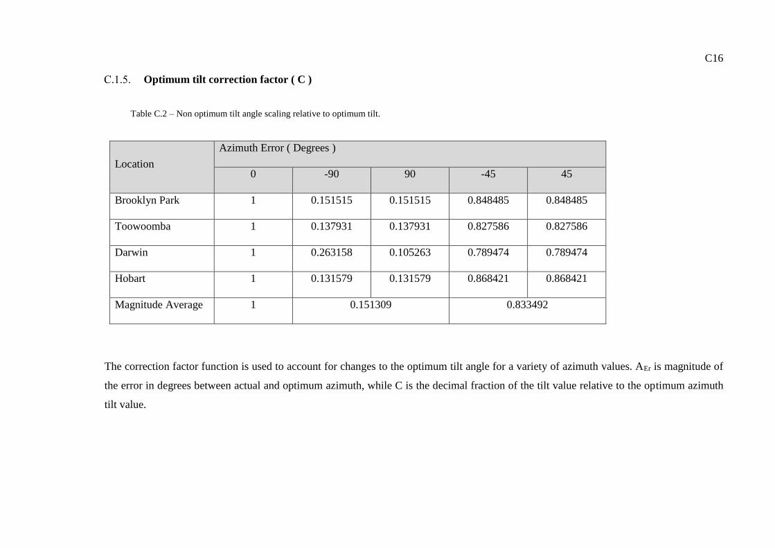
C16
Optimum tilt correction factor ( C )
Table C.2 – Non optimum tilt angle scaling relative to optimum tilt.
Location
Azimuth Error ( Degrees )
0 -90 90 -45 45
Brooklyn Park 1 0.151515 0.151515 0.848485 0.848485
Toowoomba 1 0.137931 0.137931 0.827586 0.827586
Darwin 1 0.263158 0.105263 0.789474 0.789474
Hobart 1 0.131579 0.131579 0.868421 0.868421
Magnitude Average 1 0.151309 0.833492
The correction factor function is used to account for changes to the optimum tilt angle for a variety of azimuth values. AEr is magnitude of
the error in degrees between actual and optimum azimuth, while C is the decimal fraction of the tilt value relative to the optimum azimuth
tilt value.
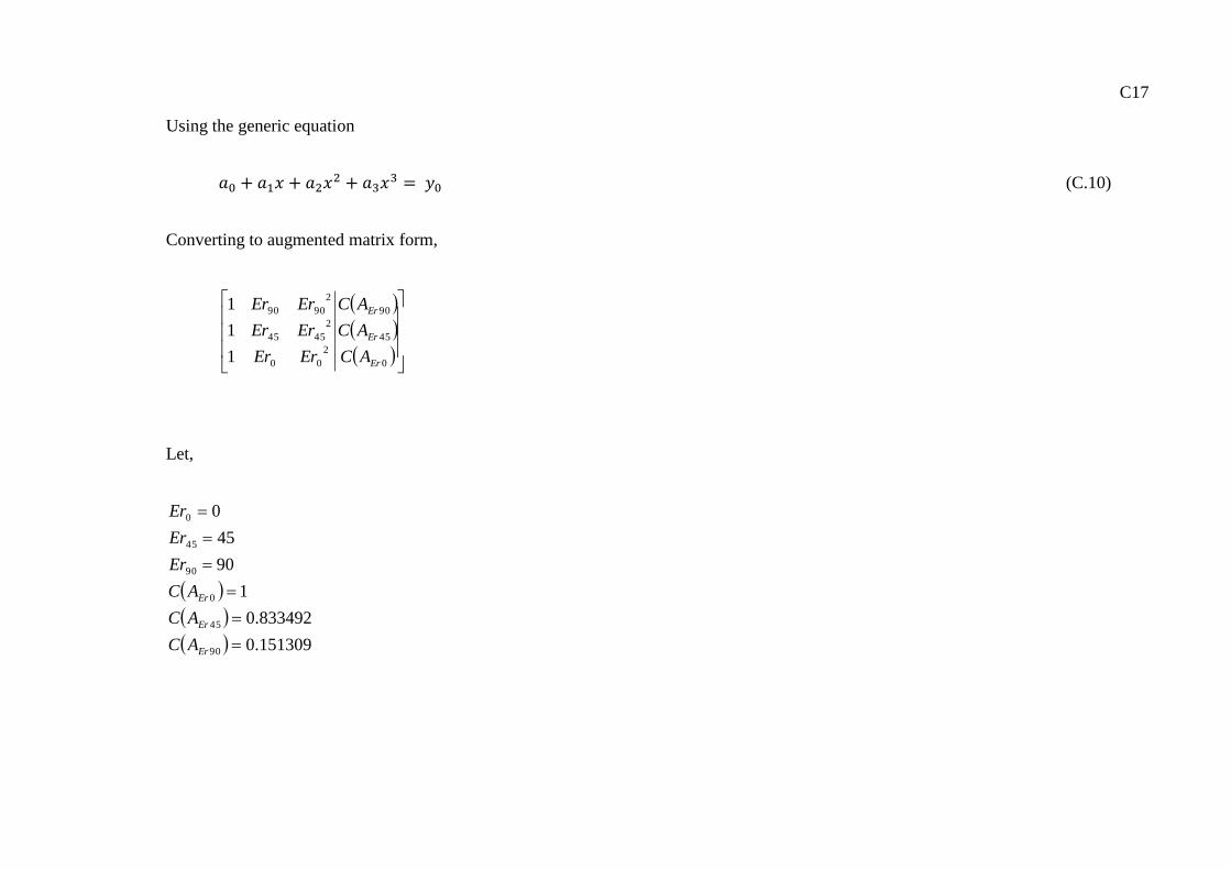
C17
Using the generic equation
𝑎0 + 𝑎1𝑥 + 𝑎2𝑥2 + 𝑎3𝑥3 = 𝑦0 (C.10)
Converting to augmented matrix form,
0
45
90
2
00
2
4545
2
9090
1
1
1
Er
Er
Er
AC
AC
AC
ErEr
ErEr
ErEr
Let,
151309.0
833492.0
1
90
45
0
90
45
0
90
45
0
Er
Er
Er
AC
AC
AC
Er
Er
Er
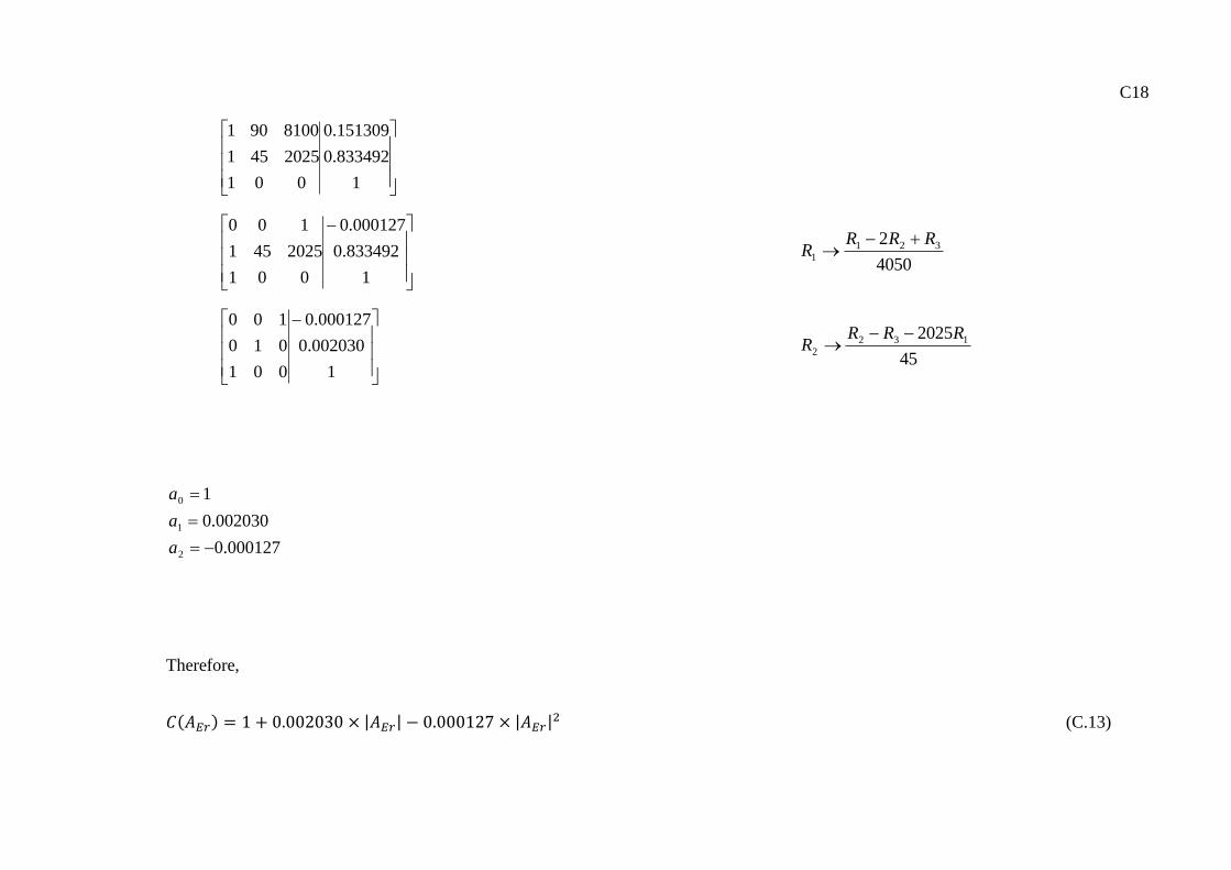
C18
1
833492.0
151309.0
001
2025451
8100901
1
833492.0
000127.0
001
2025451
100
4050
2 3211
RRRR
1
002030.0
000127.0
001
010
100
45
2025 1322
RRRR
000127.0
002030.0
1
2
1
0
a
a
a
Therefore,
𝐶(𝐴𝐸𝑟) = 1 + 0.002030 × |𝐴𝐸𝑟| − 0.000127 × |𝐴𝐸𝑟|2 (C.13)
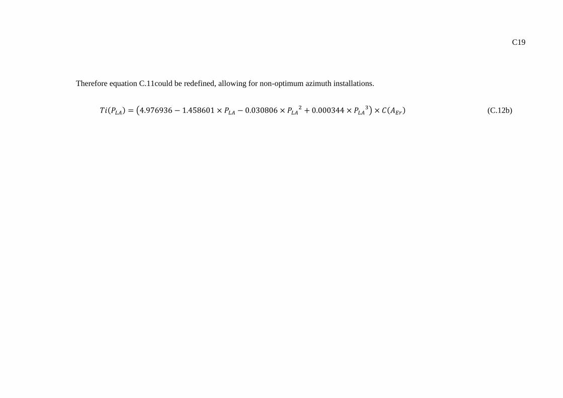
C19
Therefore equation C.11could be redefined, allowing for non-optimum azimuth installations.
𝑇𝑖(𝑃𝐿𝐴) = (4.976936 − 1.458601 × 𝑃𝐿𝐴 − 0.030806 × 𝑃𝐿𝐴2 + 0.000344 × 𝑃𝐿𝐴
3) × 𝐶(𝐴𝐸𝑟) (C.12b)

Matlab code
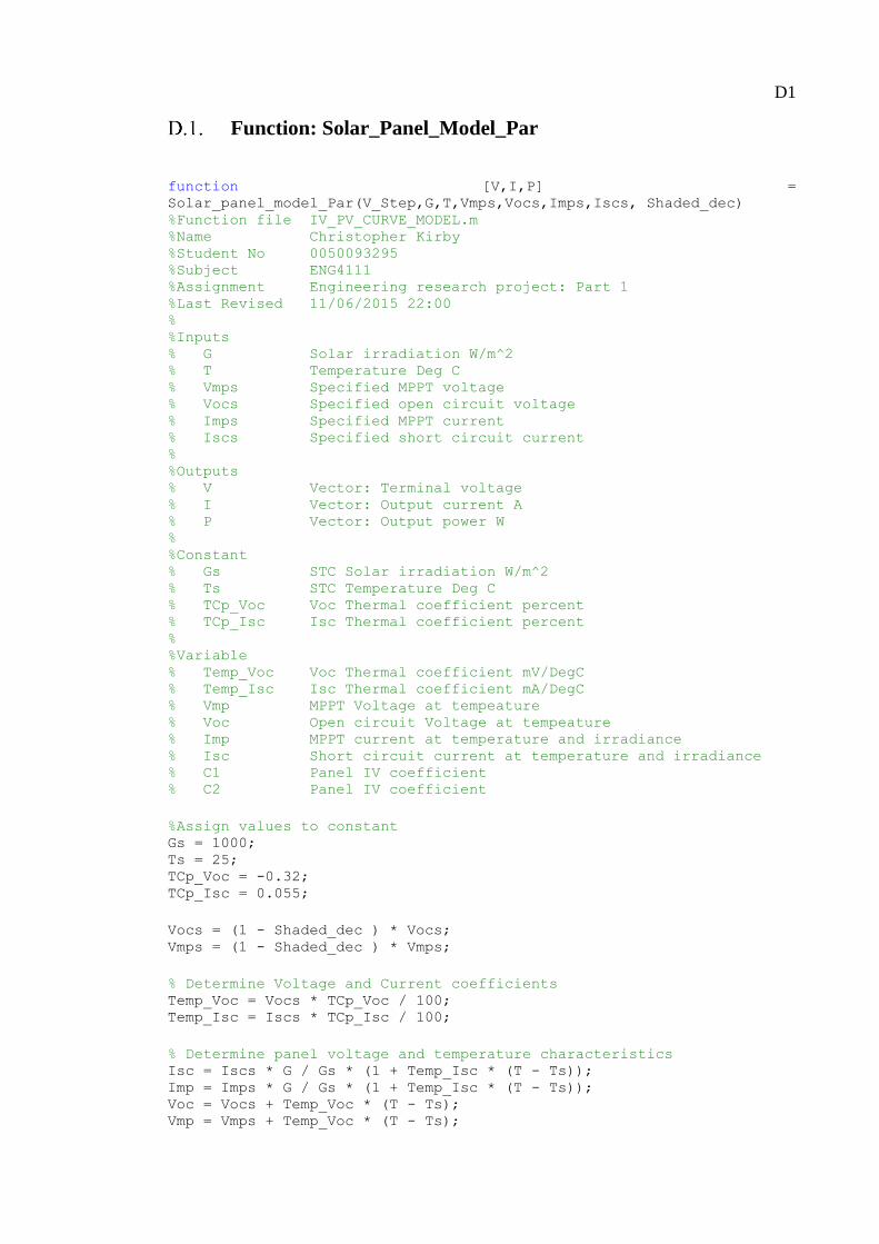
D1
Function: Solar_Panel_Model_Par
function [V,I,P] =
Solar_panel_model_Par(V_Step,G,T,Vmps,Vocs,Imps,Iscs, Shaded_dec) %Function file IV_PV_CURVE_MODEL.m %Name Christopher Kirby %Student No 0050093295 %Subject ENG4111 %Assignment Engineering research project: Part 1 %Last Revised 11/06/2015 22:00 % %Inputs % G Solar irradiation W/m^2 % T Temperature Deg C % Vmps Specified MPPT voltage % Vocs Specified open circuit voltage % Imps Specified MPPT current % Iscs Specified short circuit current % %Outputs % V Vector: Terminal voltage % I Vector: Output current A % P Vector: Output power W % %Constant % Gs STC Solar irradiation W/m^2 % Ts STC Temperature Deg C % TCp_Voc Voc Thermal coefficient percent % TCp_Isc Isc Thermal coefficient percent % %Variable % Temp_Voc Voc Thermal coefficient mV/DegC % Temp_Isc Isc Thermal coefficient mA/DegC % Vmp MPPT Voltage at tempeature % Voc Open circuit Voltage at tempeature % Imp MPPT current at temperature and irradiance % Isc Short circuit current at temperature and irradiance % C1 Panel IV coefficient % C2 Panel IV coefficient
%Assign values to constant Gs = 1000; Ts = 25; TCp_Voc = -0.32; TCp_Isc = 0.055;
Vocs = (1 - Shaded_dec ) * Vocs; Vmps = (1 - Shaded_dec ) * Vmps;
% Determine Voltage and Current coefficients Temp_Voc = Vocs * TCp_Voc / 100; Temp_Isc = Iscs * TCp_Isc / 100;
% Determine panel voltage and temperature characteristics Isc = Iscs * G / Gs * (1 + Temp_Isc * (T - Ts)); Imp = Imps * G / Gs * (1 + Temp_Isc * (T - Ts)); Voc = Vocs + Temp_Voc * (T - Ts); Vmp = Vmps + Temp_Voc * (T - Ts);
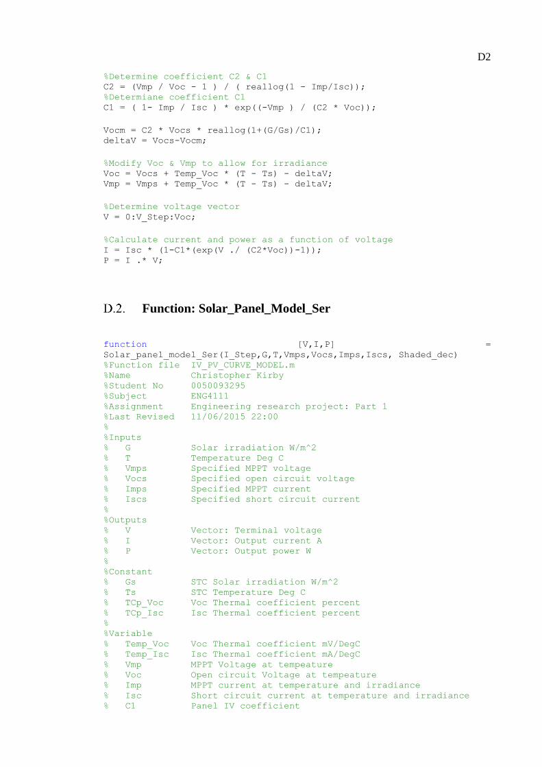
D2
%Determine coefficient C2 & C1 C2 = (Vmp / Voc - 1 ) / ( reallog(1 - Imp/Isc)); %Determiane coefficient C1 C1 = ( 1- Imp / Isc ) * exp((-Vmp ) / (C2 * Voc));
Vocm = C2 * Vocs * reallog(1+(G/Gs)/C1); deltaV = Vocs-Vocm;
%Modify Voc & Vmp to allow for irradiance Voc = Vocs + Temp_Voc * (T - Ts) - deltaV; Vmp = Vmps + Temp_Voc * (T - Ts) - deltaV;
%Determine voltage vector V = 0:V_Step:Voc;
%Calculate current and power as a function of voltage I = Isc * (1-C1*(exp(V ./ (C2*Voc))-1)); P = I .* V;
Function: Solar_Panel_Model_Ser
function [V,I,P] =
Solar_panel_model_Ser(I_Step,G,T,Vmps,Vocs,Imps,Iscs, Shaded_dec) %Function file IV_PV_CURVE_MODEL.m %Name Christopher Kirby %Student No 0050093295 %Subject ENG4111 %Assignment Engineering research project: Part 1 %Last Revised 11/06/2015 22:00 % %Inputs % G Solar irradiation W/m^2 % T Temperature Deg C % Vmps Specified MPPT voltage % Vocs Specified open circuit voltage % Imps Specified MPPT current % Iscs Specified short circuit current % %Outputs % V Vector: Terminal voltage % I Vector: Output current A % P Vector: Output power W % %Constant % Gs STC Solar irradiation W/m^2 % Ts STC Temperature Deg C % TCp_Voc Voc Thermal coefficient percent % TCp_Isc Isc Thermal coefficient percent % %Variable % Temp_Voc Voc Thermal coefficient mV/DegC % Temp_Isc Isc Thermal coefficient mA/DegC % Vmp MPPT Voltage at tempeature % Voc Open circuit Voltage at tempeature % Imp MPPT current at temperature and irradiance % Isc Short circuit current at temperature and irradiance % C1 Panel IV coefficient
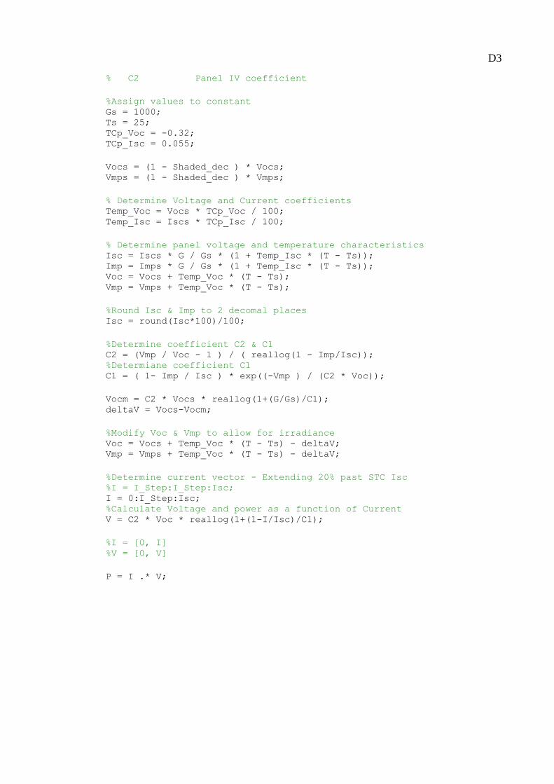
D3
% C2 Panel IV coefficient
%Assign values to constant Gs = 1000; Ts = 25; TCp_Voc = -0.32; TCp_Isc = 0.055;
Vocs = (1 - Shaded_dec ) * Vocs; Vmps = (1 - Shaded_dec ) * Vmps;
% Determine Voltage and Current coefficients Temp_Voc = Vocs * TCp_Voc / 100; Temp_Isc = Iscs * TCp_Isc / 100;
% Determine panel voltage and temperature characteristics Isc = Iscs * G / Gs * (1 + Temp_Isc * (T - Ts)); Imp = Imps * G / Gs * (1 + Temp_Isc * (T - Ts)); Voc = Vocs + Temp_Voc * (T - Ts); Vmp = Vmps + Temp_Voc * (T - Ts);
%Round Isc & Imp to 2 decomal places Isc = round(Isc*100)/100;
%Determine coefficient C2 & C1 C2 = (Vmp / Voc - 1 ) / ( reallog(1 - Imp/Isc)); %Determiane coefficient C1 C1 = ( 1- Imp / Isc ) * exp((-Vmp ) / (C2 * Voc));
Vocm = C2 * Vocs * reallog(1+(G/Gs)/C1); deltaV = Vocs-Vocm;
%Modify Voc & Vmp to allow for irradiance Voc = Vocs + Temp_Voc * (T - Ts) - deltaV; Vmp = Vmps + Temp_Voc * (T - Ts) - deltaV;
%Determine current vector - Extending 20% past STC Isc %I = I_Step:I_Step:Isc; I = 0:I_Step:Isc; %Calculate Voltage and power as a function of Current V = C2 * Voc * reallog(1+(1-I/Isc)/C1);
%I = [0, I] %V = [0, V]
P = I .* V;
D4
Script: Efficiency_calculator_Par
%Script file Efficiency_calculator_Par.m %Name Christopher Kirby %Student No 0050093295 %Subject ENG4111 %Assignment Engineering research project %Last Revised 11/06/2015 22:00 % % %%%%%%%%%%%%%%%%%%%%%%%%%%%%%%%%%%%%%%%%%%%%%%%%%%%%%%%%%%%%%%%%%%%%%%
%%%%% %clear all variables %%%%%%%%%%%%%%%%%%%%%%%%%%%%%%%%%%%%%%%%%%%%%%%%%%%%%%%%%%%%%%%%%%%%%%
%%%%% clear all
%%%%%%%%%%%%%%%%%%%%%%%%%%%%%%%%%%%%%%%%%%%%%%%%%%%%%%%%%%%%%%%%%%%%%%
%%%%% %define and calculate fixed variables %%%%%%%%%%%%%%%%%%%%%%%%%%%%%%%%%%%%%%%%%%%%%%%%%%%%%%%%%%%%%%%%%%%%%%
%%%%% P1_Angle = input('Enter Panel 1 angle: ') %Panel
angles to light source P2_Angle = 0;
P1_Modules = 3; %Number
of modules within panel P2_Modules = 3;
P1_Shaded_Modules = input('Enter Panel 1 number of shaded modules: ')
%Number of hard shaded panels P2_Shaded_Modules = input('Enter Panel 2 number of shaded modules: ')
P1_Shaded_dec = ( P1_Shaded_Modules / P1_Modules );
%Calculate percent of shaded modules as a decimal value P2_Shaded_dec = ( P2_Shaded_Modules / P2_Modules );
G = input('Enter simulated irradiance value: ')
%Simulation irradiance T = input('Enter simulated temperature: ')
%Simulation temperature
Vmps1 = input('Enter panel 1 MP Voltage: '); %Panel
1 specifications Vocs1 = input('Enter panel 1 OC Voltage: '); Imps1 = input('Enter panel 1 MP Current: '); Iscs1 = input('Enter panel 1 SC Current: '); Vmps2 = input('Enter panel 2 MP Voltage: '); %Panel
2 specifications Vocs2 = input('Enter panel 2 OC Voltage: '); Imps2 = input('Enter panel 2 MP Current: '); Iscs2 = input('Enter panel 2 SC Current: ');
K = P1_Angle; %Plot
index constant
Brewster_angle = 56.6; %Limiting
D5
angle - Brewster angle P2_Angle_Vector = []; %Rotated
panel vector V_Step = 0.1; %Voltage
vector step
MP_Sep_Vector = []; %Non
connected panel MP vector MP_Par_Vector = []; %Series
connected panel MP vector
%%%%%%%%%%%%%%%%%%%%%%%%%%%%%%%%%%%%%%%%%%%%%%%%%%%%%%%%%%%%%%%%%%%%%%
%%%%% %Model panel output %%%%%%%%%%%%%%%%%%%%%%%%%%%%%%%%%%%%%%%%%%%%%%%%%%%%%%%%%%%%%%%%%%%%%%
%%%%% while P2_Angle <= Brewster_angle; %Program
loop for angles below limit G1 = G * cos( P1_Angle *pi / 180 );
%Equlvalent irradiance due to angle G2 = G * cos( P2_Angle *pi / 180 );
%Model Panel 1: Solar panel model_Par [V1,I1,P1] =
Solar_panel_model_Par(V_Step,G1,T,Vmps1,Vocs1,Imps1,Iscs1,P1_Shaded_de
c); V1 = round(V1*100)/100; I1 = round(I1*100)/100; P1 = round(P1*100)/100; I1(I1<0)=0; P1(P1<0)=0;
%Locate actual MPPT using incremental
%method starting from panel spec MPPT P1_Pmp = 0; if max(V1) > Vmps1; index = find( V1( : ) == Vmps1 ); else index = length(V1) - 1; end while P1_Pmp == 0;
if (P1(index-1)<=P1(index) & P1(index)>=P1(index+1)); P1_Pmp = P1(index); elseif (P1(index-1)>=P1(index) & P1(index)>=P1(index+1) ); index = index - 1; elseif (P1(index-1)<=P1(index) & P1(index)<=P1(index+1)); index = index + 1; elseif (P1(index-1)>=P1(index) & P1(index)<=P1(index+1)); index = index + 1; else P1(index) = 0; index = index - 1; end end
%Model Panel 2: Solar panel model_Ser [V2,I2,P2] =
Solar_panel_model_Par(V_Step,G2,T,Vmps2,Vocs2,Imps2,Iscs2,P2_Shaded_de
D6
c); V2 = round(V2*100)/100; I2 = round(I2*100)/100; P2 = round(P2*100)/100; I2(I2<0)=0; P2(P2<0)=0;
%Locate actual MPPT using incremental
%method starting from panel spec MPPT P2_Pmp = 0; if max(V2) > Vmps2; index = find( V2( : ) == Vmps2 ); else index = length(V2) - 1; end while P2_Pmp == 0; if (P2(index-1)<=P2(index) & P2(index)>=P2(index+1)); P2_Pmp = P2(index); elseif (P2(index-1)>=P2(index) & P2(index)>=P2(index+1)); index = index - 1; elseif (P2(index-1)<=P2(index) & P2(index)<=P2(index+1)); index = index + 1; elseif (P2(index-1)>=P2(index) & P2(index)<=P2(index+1)); index = index + 1; else P2(index) = 0; index = index - 1; end end
difference = abs(length (V1) - length (V2));
%Standardise vector lengths zero_vector = zeros(1,difference); if length (V1) < length (V2); V1 = V2; I1 = [I1,zero_vector]; P1 = [P1,zero_vector]; end if length (V1) > length (V2); V2 = V1; I2 = [I2,zero_vector]; P2 = [P2,zero_vector]; end
%%%%%%%%%%%%%%%%%%%%%%%%%%%%%%%%%%%%%%%%%%%%%%%%%%%%%%%%%%%%%%%%%%%%%%
%%%%% %MODEL PARALLEL COMBINATION %%%%%%%%%%%%%%%%%%%%%%%%%%%%%%%%%%%%%%%%%%%%%%%%%%%%%%%%%%%%%%%%%%%%%%
%%%%% Vparallel = V1; Iparallel = I1 + I2; Pparallel = Vparallel .* Iparallel; Vparallel = round(Vparallel*100)/100; Iparallel = round(Iparallel*100)/100; Pparallel = round(Pparallel*100)/100;
Parallel_Pmp = 0; while Parallel_Pmp == 0; if (Pparallel(index-1)<=Pparallel(index) &
D7
Pparallel(index)>=Pparallel(index+1)); Parallel_Pmp = Pparallel(index); elseif (Pparallel(index-1)>=Pparallel(index) &
Pparallel(index)>=Pparallel(index+1)); index = index - 1; elseif (Pparallel(index-1)<=Pparallel(index) &
Pparallel(index)<=Pparallel(index+1)); index = index + 1; elseif (Pparallel(index-1)>=Pparallel(index) &
Pparallel(index)<=Pparallel(index+1)); index = index + 1; else Pparallel(index) = 0; index = index - 1; end end
%%%%%%%%%%%%%%%%%%%%%%%%%%%%%%%%%%%%%%%%%%%%%%%%%%%%%%%%%%%%%%%%%%%%%%
%%%%% %PLOT RESULTING IV / PV curves for P1, P2 & Parallel COMBINATION %%%%%%%%%%%%%%%%%%%%%%%%%%%%%%%%%%%%%%%%%%%%%%%%%%%%%%%%%%%%%%%%%%%%%%
%%%%% subplot(2,11,1:4); plt = plotyy (V1,I1,V1,P1); title('Panel 1: IV & PV'); xlabel('Voltage (V)'); ylabel(plt(1), 'Current (A)'); ylabel(plt(2), 'Power (W)');
subplot(2,11,8:11); plt = plotyy (V2,I2,V2,P2); title('Panel 2: IV & PV'); xlabel('Voltage (V)'); ylabel(plt(1), 'Current (A)'); ylabel(plt(2), 'Power (W)');
subplot(2,11,12:22); plt = plotyy (Vparallel,Iparallel,Vparallel,Pparallel); title('Parallel: IV & PV'); xlabel('Voltage (V)'); ylabel(plt(1), 'Current (A)'); ylabel(plt(2), 'Power (W)');
%%%%%%%%%%%%%%%%%%%%%%%%%%%%%%%%%%%%%%%%%%%%%%%%%%%%%%%%%%%%%%%%%%%%%%
%%%%% %SAVE PLOT IMAGE at 10 degree INCREMENTS %%%%%%%%%%%%%%%%%%%%%%%%%%%%%%%%%%%%%%%%%%%%%%%%%%%%%%%%%%%%%%%%%%%%%%
%%%%% if P2_Angle == 0; K=K+1; print('-djpeg',sprintf('IV_PAR%d',K)); end;
if P2_Angle == 10; K=K+1; print('-djpeg',sprintf('IV_PAR%d',K)); end;
if P2_Angle == 20; K=K+1; print('-djpeg',sprintf('IV_PAR%d',K));
D8
end;
if P2_Angle == 30; K=K+1; print('-djpeg',sprintf('IV_PAR%d',K)); end;
if P2_Angle == 40; K=K+1; print('-djpeg',sprintf('IV_PAR%d',K)); end;
if P2_Angle == 50; K=K+1; print('-djpeg',sprintf('IV_PAR%d',K)); end;
if P2_Angle == 56; K=K+1; print('-djpeg',sprintf('IV_PAR%d',K)); end;
%%%%%%%%%%%%%%%%%%%%%%%%%%%%%%%%%%%%%%%%%%%%%%%%%%%%%%%%%%%%%%%%%%%%%%
%%%%% %CALCULATE MAX POWER AND EFFICIENCY VECTORS %%%%%%%%%%%%%%%%%%%%%%%%%%%%%%%%%%%%%%%%%%%%%%%%%%%%%%%%%%%%%%%%%%%%%%
%%%%% MP_Seperate = P1_Pmp + P2_Pmp; %Non
connected panel MP MP_Parallel = Parallel_Pmp; %Parallel
connected panel MP %
%Efficiency vector Percent_Eff_to_Seperate(P2_Angle+1) = Parallel_Pmp / (P1_Pmp + P2_Pmp)
* 100; %
P2_Angle_Vector = [P2_Angle_Vector,P2_Angle]; %Panel
angle vector P2_Angle = P2_Angle + 1; %Increment
panel 2 angle
MP_Sep_Vector = [MP_Sep_Vector , MP_Seperate]; %Non
connected panel MP vector MP_Par_Vector = [MP_Par_Vector , MP_Parallel];
%Series connected panel MP vector % end
%%%%%%%%%%%%%%%%%%%%%%%%%%%%%%%%%%%%%%%%%%%%%%%%%%%%%%%%%%%%%%%%%%%%%%
%%%%% %PLOT MAX POWER Versus ANGLE %%%%%%%%%%%%%%%%%%%%%%%%%%%%%%%%%%%%%%%%%%%%%%%%%%%%%%%%%%%%%%%%%%%%%%
%%%%% % clf %Clear
plot Window plt = plotyy ( P2_Angle_Vector, [MP_Sep_Vector.'
MP_Par_Vector.'],P2_Angle_Vector,MP_Sep_Vector- MP_Par_Vector);
D9
title(sprintf('Panel output power vs Angle ( Panel 1 Angle %d degrees
)', P1_Angle)); %title(sprintf('Panel output power vs Angle ( Ambient temperature %d
degrees C )', T)); %title(sprintf('Panel output power vs Angle ( Irradiance %d W/m^2 )',
G)); %title(sprintf('Panel output power vs Angle'));
xlabel('Panel 2 Angle from solar normal'); ylabel(plt(1), 'Panel output power (W)'); ylabel(plt(2), 'Parallel connected power loss (W)');
K=K+1; print('-djpeg',sprintf('IV_PAR%d',K)); %Save Angle versus MP plot
Script: Efficiency_calculator_Ser
%Script file Efficiency_calculator_Ser.m %Name Christopher Kirby %Student No 0050093295 %Subject ENG4111 %Assignment Engineering research project %Last Revised 11/06/2015 22:00 % % %%%%%%%%%%%%%%%%%%%%%%%%%%%%%%%%%%%%%%%%%%%%%%%%%%%%%%%%%%%%%%%%%%%%%%
%%%%% %clear all variables %%%%%%%%%%%%%%%%%%%%%%%%%%%%%%%%%%%%%%%%%%%%%%%%%%%%%%%%%%%%%%%%%%%%%%
%%%%% clear all
%%%%%%%%%%%%%%%%%%%%%%%%%%%%%%%%%%%%%%%%%%%%%%%%%%%%%%%%%%%%%%%%%%%%%%
%%%%% %define and calculate fixed variables %%%%%%%%%%%%%%%%%%%%%%%%%%%%%%%%%%%%%%%%%%%%%%%%%%%%%%%%%%%%%%%%%%%%%%
%%%%% P1_Angle = input('Enter Panel 1 angle: ') %Panel
angles to light source P2_Angle = 0;
P1_Modules = 3; %Number
of modules within panel P2_Modules = 3;
P1_Shaded_Modules = input('Enter Panel 1 number of shaded modules: ')
%Number of hard shaded panels P2_Shaded_Modules = input('Enter Panel 2 number of shaded modules: ')
P1_Shaded_dec = ( P1_Shaded_Modules / P1_Modules );
%Calculate percent of shaded modules as a decimal value P2_Shaded_dec = ( P2_Shaded_Modules / P2_Modules );
D10
G = input('Enter simulated irradiance value: ')
%Simulation irradiance T = input('Enter simulated temperature: ')
%Simulation temperature
Vmps1 = input('Enter panel 1 MP Voltage: '); %Panel
1 specifications Vocs1 = input('Enter panel 1 OC Voltage: '); Imps1 = input('Enter panel 1 MP Current: '); Iscs1 = input('Enter panel 1 SC Current: '); Vmps2 = input('Enter panel 2 MP Voltage: '); %Panel
2 specifications Vocs2 = input('Enter panel 2 OC Voltage: '); Imps2 = input('Enter panel 2 MP Current: '); Iscs2 = input('Enter panel 2 SC Current: ');
K = P1_Angle; %Plot
index constant
Brewster_angle = 56.6; %Limiting
angle - Brewster angle P2_Angle_Vector = []; %Rotated
panel vector I_Step = 0.01; %Current
vector step
MP_Sep_Vector = []; %Non
connected panel MP vector MP_Ser_Vector = []; %Series
connected panel MP vector
%%%%%%%%%%%%%%%%%%%%%%%%%%%%%%%%%%%%%%%%%%%%%%%%%%%%%%%%%%%%%%%%%%%%%%
%%%%% %Model panel output %%%%%%%%%%%%%%%%%%%%%%%%%%%%%%%%%%%%%%%%%%%%%%%%%%%%%%%%%%%%%%%%%%%%%%
%%%%% while P2_Angle <= Brewster_angle; %Program
loop for angles below limit G1 = G * cos( P1_Angle *pi / 180 );
%Equlvalent irradiance due to angle G2 = G * cos( P2_Angle *pi / 180 );
%Model Panel 1: Solar panel model_Ser [V1,I1,P1] =
Solar_panel_model_Ser(I_Step,G1,T,Vmps1,Vocs1,Imps1,Iscs1,P1_Shaded_de
c); V1 = round(V1*100)/100; I1 = round(I1*100)/100; P1 = round(P1*100)/100; I1(I1<0)=0; P1(P1<0)=0;
%Locate actual MPPT using incremental
%method starting from panel spec MPPT P1_Pmp = 0; if max(I1) > Imps1; index = find( I1( : ) == Imps1 ); else index = length(I1) - 1; end
D11
while P1_Pmp == 0;
if (P1(index-1)<=P1(index) & P1(index)>=P1(index+1)); P1_Pmp = P1(index); elseif (P1(index-1)>=P1(index) & P1(index)>=P1(index+1) ); index = index - 1; elseif (P1(index-1)<=P1(index) & P1(index)<=P1(index+1)); index = index + 1; else P1(index) = 0; index = index - 1; end end
%Model Panel 2: Solar panel model_Ser [V2,I2,P2] =
Solar_panel_model_Ser(I_Step,G2,T,Vmps2,Vocs2,Imps2,Iscs2,P2_Shaded_de
c); V2 = round(V2*100)/100; I2 = round(I2*100)/100; P2 = round(P2*100)/100; I2(I2<0)=0; P2(P2<0)=0;
%Locate actual MPPT using incremental
%method starting from panel spec MPPT P2_Pmp = 0; if max(I2) > Imps2; index = find( I2( : ) == Imps2 ); else index = length(I2) - 1; end while P2_Pmp == 0; if (P2(index-1)<=P2(index) & P2(index)>=P2(index+1)); P2_Pmp = P2(index); elseif (P2(index-1)>=P2(index) & P2(index)>=P2(index+1)); index = index - 1; elseif (P2(index-1)<=P2(index) & P2(index)<=P2(index+1)); index = index + 1; else P2(index) = 0; index = index - 1; end end
difference = abs(length (I1) - length (I2));
%Standardise vector lengths zero_vector = zeros(1,difference); if length (I1) < length (I2); I1 = I2; V1 = [V1,zero_vector]; P1 = [P1,zero_vector]; end if length (I1) > length (I2); I2 = I1; V2 = [V2,zero_vector]; P2 = [P2,zero_vector]; end
D12
%%%%%%%%%%%%%%%%%%%%%%%%%%%%%%%%%%%%%%%%%%%%%%%%%%%%%%%%%%%%%%%%%%%%%%
%%%%% %MODEL SERIES COMBINATION %%%%%%%%%%%%%%%%%%%%%%%%%%%%%%%%%%%%%%%%%%%%%%%%%%%%%%%%%%%%%%%%%%%%%%
%%%%% Vseries = V1 + V2; Iseries = I1; Pseries = Vseries .* Iseries; Vseries = round(Vseries*100)/100; Iseries = round(Iseries*100)/100; Pseries = round(Pseries*100)/100;
index = 2; Series_Pmp = 0; while Series_Pmp == 0; if (Pseries(index-1)<=Pseries(index) &
Pseries(index)>=Pseries(index+1)); Series_Pmp = Pseries(index); elseif (Pseries(index-1)>=Pseries(index) &
Pseries(index)>=Pseries(index+1) ); index = index - 1; elseif (Pseries(index-1)<=Pseries(index) &
Pseries(index)<=Pseries(index+1)); index = index + 1; else Pseries(index) = 0; index = index - 1; end end
%%%%%%%%%%%%%%%%%%%%%%%%%%%%%%%%%%%%%%%%%%%%%%%%%%%%%%%%%%%%%%%%%%%%%%
%%%%% %PLOT RESULTING IV / PV curves for P1, P2 & SERIES COMBINATION %%%%%%%%%%%%%%%%%%%%%%%%%%%%%%%%%%%%%%%%%%%%%%%%%%%%%%%%%%%%%%%%%%%%%%
%%%%% subplot(2,11,1:4); plt = plotyy (V1,I1,V1,P1); title('Panel 1: IV & PV'); xlabel('Voltage (V)'); ylabel(plt(1), 'Current (A)'); ylabel(plt(2), 'Power (W)');
subplot(2,11,8:11); plt = plotyy (V2,I2,V2,P2); title('Panel 2: IV & PV'); xlabel('Voltage (V)'); ylabel(plt(1), 'Current (A)'); ylabel(plt(2), 'Power (W)');
subplot(2,11,12:22); plt = plotyy (Vseries,Iseries,Vseries,Pseries); title('Series: IV & PV'); xlabel('Voltage (V)'); ylabel(plt(1), 'Current (A)'); ylabel(plt(2), 'Power (W)');
%%%%%%%%%%%%%%%%%%%%%%%%%%%%%%%%%%%%%%%%%%%%%%%%%%%%%%%%%%%%%%%%%%%%%%
%%%%% %SAVE PLOT IMAGE at 10 degree INCREMENTS %%%%%%%%%%%%%%%%%%%%%%%%%%%%%%%%%%%%%%%%%%%%%%%%%%%%%%%%%%%%%%%%%%%%%%
D13
%%%%% if P2_Angle == 0; K=K+1; print('-djpeg',sprintf('IV_SER%d',K)); end;
if P2_Angle == 10; K=K+1; print('-djpeg',sprintf('IV_SER%d',K)); end;
if P2_Angle == 20; K=K+1; print('-djpeg',sprintf('IV_SER%d',K)); end;
if P2_Angle == 30; K=K+1; print('-djpeg',sprintf('IV_SER%d',K)); end;
if P2_Angle == 40; K=K+1; print('-djpeg',sprintf('IV_SER%d',K)); end;
if P2_Angle == 50; K=K+1; print('-djpeg',sprintf('IV_SER%d',K)); end;
if P2_Angle == 56; K=K+1; print('-djpeg',sprintf('IV_SER%d',K)); end;
%%%%%%%%%%%%%%%%%%%%%%%%%%%%%%%%%%%%%%%%%%%%%%%%%%%%%%%%%%%%%%%%%%%%%%
%%%%% %CALCULATE MAX POWER AND EFFICIENCY VECTORS %%%%%%%%%%%%%%%%%%%%%%%%%%%%%%%%%%%%%%%%%%%%%%%%%%%%%%%%%%%%%%%%%%%%%%
%%%%% MP_Seperate = P1_Pmp + P2_Pmp; %Non
connected panel MP MP_Series = Series_Pmp; %Series
connected panel MP
%Efficiency vector Percent_Eff_to_Seperate(P2_Angle+1) = Series_Pmp / (P1_Pmp + P2_Pmp) *
100;
P2_Angle_Vector = [P2_Angle_Vector,P2_Angle]; %Panel
angle vector P2_Angle = P2_Angle + 1; %Increment
panel 2 angle
MP_Sep_Vector = [MP_Sep_Vector , MP_Seperate]; %Non
connected panel MP vector MP_Ser_Vector = [MP_Ser_Vector , MP_Series];
D14
%Series connected panel MP vector % end
%%%%%%%%%%%%%%%%%%%%%%%%%%%%%%%%%%%%%%%%%%%%%%%%%%%%%%%%%%%%%%%%%%%%%%
%%%%% %PLOT MAX POWER Versus ANGLE %%%%%%%%%%%%%%%%%%%%%%%%%%%%%%%%%%%%%%%%%%%%%%%%%%%%%%%%%%%%%%%%%%%%%%
%%%%% % clf %Clear
plot Window plt = plotyy ( P2_Angle_Vector, [MP_Sep_Vector.'
MP_Ser_Vector.'],P2_Angle_Vector,MP_Sep_Vector- MP_Ser_Vector);
title(sprintf('Panel output power vs Angle ( Panel 1 Angle %d degrees
)', P1_Angle)); %title(sprintf('Panel output power vs Angle ( Ambient temperature %d
degrees C )', T)); %title(sprintf('Panel output power vs Angle ( Irradiance %d W/m^2 )',
G)); %title(sprintf('Panel output power vs Angle'));
xlabel('Panel 2 Angle from solar normal'); ylabel(plt(1), 'Panel output power (W)'); ylabel(plt(2), 'Series connected power loss (W)');
K=K+1; print('-djpeg',sprintf('IV_SER%d',K)); %Save
Angle versus MP plot
Script: Error Search
%Sctript file Error_Search.m %Name Christopher Kirby %Student No 0050093295 %Subject ENG4111 %Assignment Engineering research project %Last Revised 14/06/2015 10:30 % %
%Define panel specifications and standard test conditions G=1000 Gs=1000 T = 25 Vmps = 35.4 Vocs = 44.6 Imps = 4.95 Iscs = 5.30
%%%%%%%%%%%%%%%%%%%%%%%%%%%%%%%%%%%%%%%%%%%%%%%%%%%%%%%%%%%%%%%%%%%%%%
%%%%% %MODEL IV CURVE
D15
%%%%%%%%%%%%%%%%%%%%%%%%%%%%%%%%%%%%%%%%%%%%%%%%%%%%%%%%%%%%%%%%%%%%%%
%%%%% [V,I,P,C1,C2] = Solar_panel_model(G,T,Vmps,Vocs,Imps,Iscs)
%Set Irradiance vector G = 0:1000;
%Calculate value for modified open circuit voltage Vocm = C2 * Vocs * reallog(1+(1-G/Gs)/C1) %Calculate open circuit voltage change deltaV = Vocs-Vocm
%%%%%%%%%%%%%%%%%%%%%%%%%%%%%%%%%%%%%%%%%%%%%%%%%%%%%%%%%%%%%%%%%%%%%%
%%%%% %PLOT CALCULATED IV CURVE VALUES %%%%%%%%%%%%%%%%%%%%%%%%%%%%%%%%%%%%%%%%%%%%%%%%%%%%%%%%%%%%%%%%%%%%%%
%%%%% plot (G , Vocm ,'r') xlabel('Irradiance (W/m²)') ylabel('Open circuit voltage (V)') set(gca,'XTick',[0:100:1000]) set(gca,'YTick',[0:5:60])
Script: Varied_Irradiance_Plot
%Sctript file Varied_Irradiance_Plot.m %Name Christopher Kirby %Student No 0050093295 %Subject ENG4111 %Assignment Engineering research project: Part 1 %Last Revised 14/06/2015 10:30 % %Define panel specifications and standard test conditions T = 25 Vmps = 35.4 Vocs = 44.6 Imps = 4.95 Iscs = 5.30
%%%%%%%%%%%%%%%%%%%%%%%%%%%%%%%%%%%%%%%%%%%%%%%%%%%%%%%%%%%%%%%%%%%%%%
%%%%% %MODEL IV CURVE %%%%%%%%%%%%%%%%%%%%%%%%%%%%%%%%%%%%%%%%%%%%%%%%%%%%%%%%%%%%%%%%%%%%%%
%%%%% [V1000,I1000,P1000] =
Solar_panel_model_Par(0.1,1000,T,Vmps,Vocs,Imps,Iscs,0) I1000(I1000<0)=0
[V800,I800,P800] =
Solar_panel_model_Par(0.1,800,T,Vmps,Vocs,Imps,Iscs,0) I800(I800<0)=0
[V600,I600,P600] =
Solar_panel_model_Par(0.1,600,T,Vmps,Vocs,Imps,Iscs,0) I600(I600<0)=0
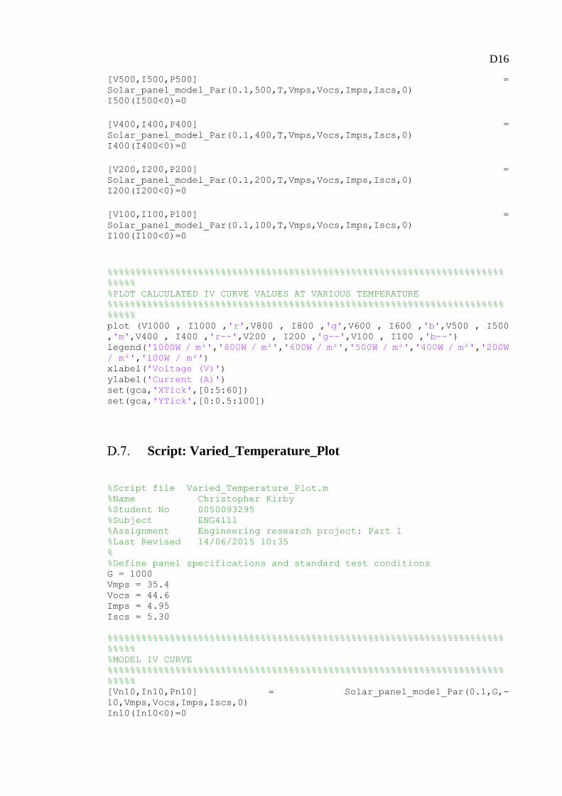
D16
[V500,I500,P500] =
Solar_panel_model_Par(0.1,500,T,Vmps,Vocs,Imps,Iscs,0) I500(I500<0)=0
[V400,I400,P400] =
Solar_panel_model_Par(0.1,400,T,Vmps,Vocs,Imps,Iscs,0) I400(I400<0)=0
[V200,I200,P200] =
Solar_panel_model_Par(0.1,200,T,Vmps,Vocs,Imps,Iscs,0) I200(I200<0)=0
[V100,I100,P100] =
Solar_panel_model_Par(0.1,100,T,Vmps,Vocs,Imps,Iscs,0) I100(I100<0)=0
%%%%%%%%%%%%%%%%%%%%%%%%%%%%%%%%%%%%%%%%%%%%%%%%%%%%%%%%%%%%%%%%%%%%%%
%%%%% %PLOT CALCULATED IV CURVE VALUES AT VARIOUS TEMPERATURE %%%%%%%%%%%%%%%%%%%%%%%%%%%%%%%%%%%%%%%%%%%%%%%%%%%%%%%%%%%%%%%%%%%%%%
%%%%% plot (V1000 , I1000 ,'r',V800 , I800 ,'g',V600 , I600 ,'b',V500 , I500
,'m',V400 , I400 ,'r--',V200 , I200 ,'g--',V100 , I100 ,'b--') legend('1000W / m²','800W / m²','600W / m²','500W / m²','400W / m²','200W
/ m²','100W / m²') xlabel('Voltage (V)') ylabel('Current (A)') set(gca,'XTick',[0:5:60]) set(gca,'YTick',[0:0.5:100])
Script: Varied_Temperature_Plot
%Script file Varied_Temperature_Plot.m %Name Christopher Kirby %Student No 0050093295 %Subject ENG4111 %Assignment Engineering research project: Part 1 %Last Revised 14/06/2015 10:35 % %Define panel specifications and standard test conditions G = 1000 Vmps = 35.4 Vocs = 44.6 Imps = 4.95 Iscs = 5.30
%%%%%%%%%%%%%%%%%%%%%%%%%%%%%%%%%%%%%%%%%%%%%%%%%%%%%%%%%%%%%%%%%%%%%%
%%%%% %MODEL IV CURVE %%%%%%%%%%%%%%%%%%%%%%%%%%%%%%%%%%%%%%%%%%%%%%%%%%%%%%%%%%%%%%%%%%%%%%
%%%%% [Vn10,In10,Pn10] = Solar_panel_model_Par(0.1,G,-
10,Vmps,Vocs,Imps,Iscs,0) In10(In10<0)=0
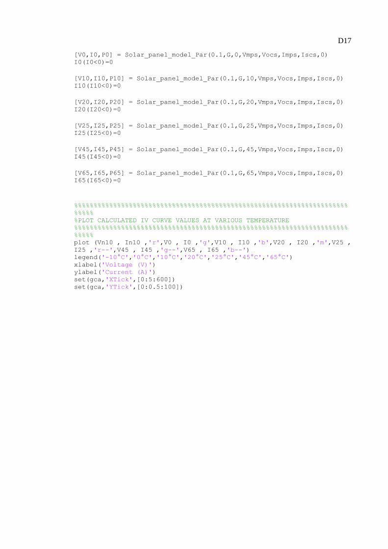
D17
[V0,I0,P0] = Solar_panel_model_Par(0.1,G,0,Vmps,Vocs,Imps,Iscs,0) I0(I0<0)=0
[V10,I10,P10] = Solar_panel_model_Par(0.1,G,10,Vmps,Vocs,Imps,Iscs,0) I10(I10<0)=0
[V20,I20,P20] = Solar_panel_model_Par(0.1,G,20,Vmps,Vocs,Imps,Iscs,0) I20(I20<0)=0
[V25,I25,P25] = Solar_panel_model_Par(0.1,G,25,Vmps,Vocs,Imps,Iscs,0) I25(I25<0)=0
[V45,I45,P45] = Solar_panel_model_Par(0.1,G,45,Vmps,Vocs,Imps,Iscs,0) I45(I45<0)=0
[V65,I65,P65] = Solar_panel_model_Par(0.1,G,65,Vmps,Vocs,Imps,Iscs,0) I65(I65<0)=0
%%%%%%%%%%%%%%%%%%%%%%%%%%%%%%%%%%%%%%%%%%%%%%%%%%%%%%%%%%%%%%%%%%%%%%
%%%%% %PLOT CALCULATED IV CURVE VALUES AT VARIOUS TEMPERATURE %%%%%%%%%%%%%%%%%%%%%%%%%%%%%%%%%%%%%%%%%%%%%%%%%%%%%%%%%%%%%%%%%%%%%%
%%%%% plot (Vn10 , In10 ,'r',V0 , I0 ,'g',V10 , I10 ,'b',V20 , I20 ,'m',V25 ,
I25 ,'r--',V45 , I45 ,'g--',V65 , I65 ,'b--') legend('-10°C','0°C','10°C','20°C','25°C','45°C','65°C') xlabel('Voltage (V)') ylabel('Current (A)') set(gca,'XTick',[0:5:600]) set(gca,'YTick',[0:0.5:100])

Modelling results
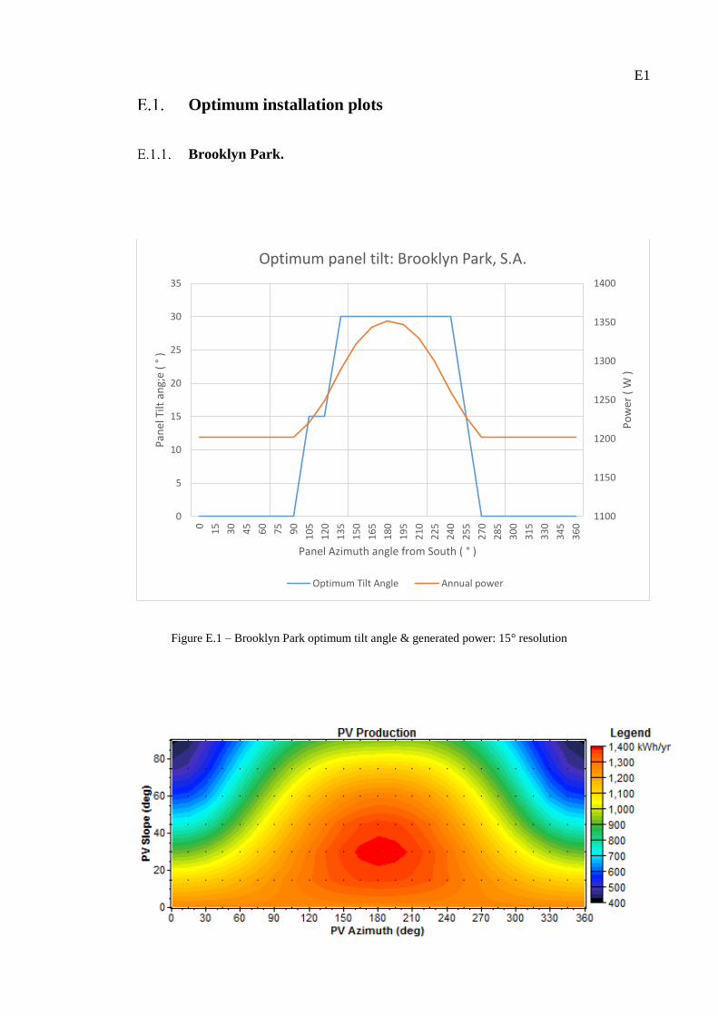
E1
Optimum installation plots
Brooklyn Park.
Figure E.1 – Brooklyn Park optimum tilt angle & generated power: 15° resolution
1100
1150
1200
1250
1300
1350
1400
0
5
10
15
20
25
30
35
0
15
30
45
60
75
90
10
5
12
0
13
5
15
0
16
5
18
0
19
5
21
0
22
5
24
0
25
5
27
0
28
5
30
0
31
5
33
0
34
5
36
0
Po
wer
( W
)
Pan
el T
ilt a
ng;
e (
°)
Panel Azimuth angle from South ( ° )
Optimum panel tilt: Brooklyn Park, S.A.
Optimum Tilt Angle Annual power
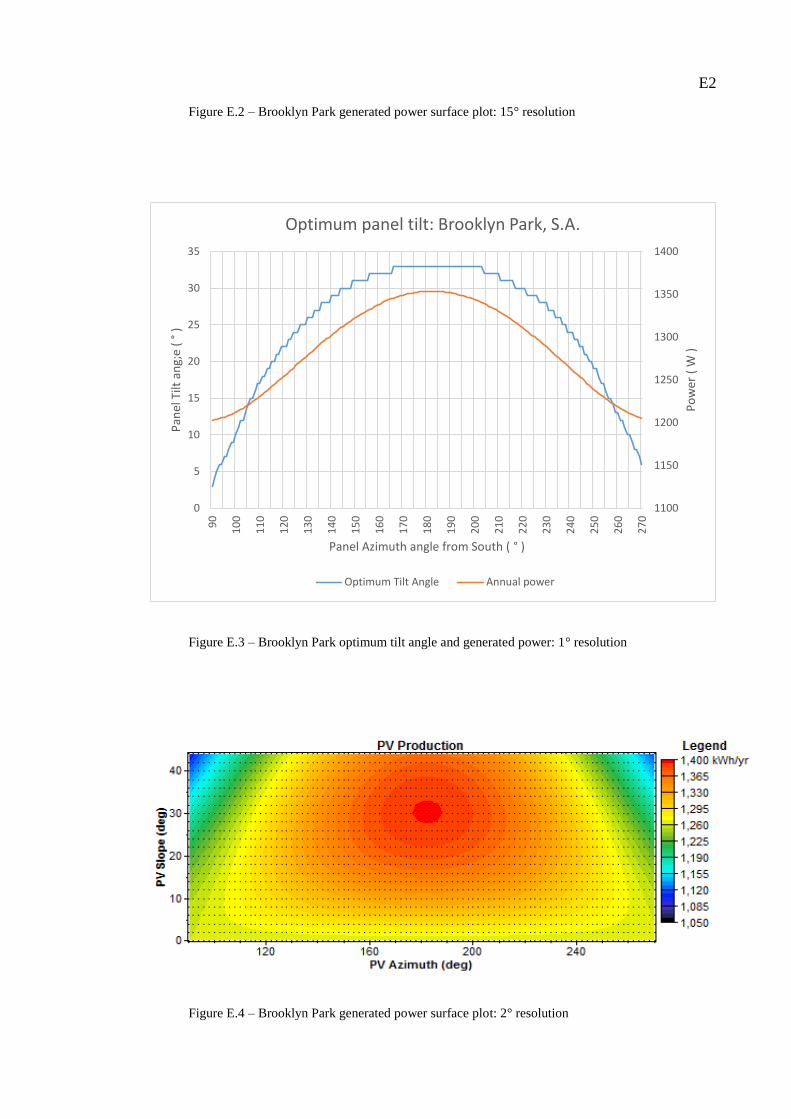
E2
Figure E.2 – Brooklyn Park generated power surface plot: 15° resolution
Figure E.3 – Brooklyn Park optimum tilt angle and generated power: 1° resolution
Figure E.4 – Brooklyn Park generated power surface plot: 2° resolution
1100
1150
1200
1250
1300
1350
1400
0
5
10
15
20
25
30
35
90
10
0
11
0
12
0
13
0
14
0
15
0
16
0
17
0
18
0
19
0
20
0
21
0
22
0
23
0
24
0
25
0
26
0
27
0
Po
wer
( W
)
Pan
el T
ilt a
ng;
e (
°)
Panel Azimuth angle from South ( ° )
Optimum panel tilt: Brooklyn Park, S.A.
Optimum Tilt Angle Annual power
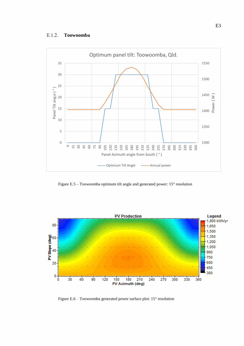
E3
Toowoomba
Figure E.5 – Toowoomba optimum tilt angle and generated power: 15° resolution
Figure E.6 – Toowoomba generated power surface plot: 15° resolution
1300
1350
1400
1450
1500
1550
0
5
10
15
20
25
30
350
15
30
45
60
75
90
10
5
12
0
13
5
15
0
16
5
18
0
19
5
21
0
22
5
24
0
25
5
27
0
28
5
30
0
31
5
33
0
34
5
36
0
Po
wer
( W
)
Pan
el T
ilt a
ng;
e (
°)
Panel Azimuth angle from South ( ° )
Optimum panel tilt: Toowoomba, Qld.
Optimum Tilt Angle Annual power
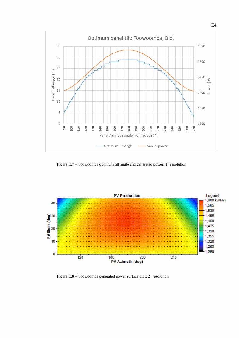
E4
Figure E.7 – Toowoomba optimum tilt angle and generated power: 1° resolution
Figure E.8 – Toowoomba generated power surface plot: 2° resolution
1300
1350
1400
1450
1500
1550
0
5
10
15
20
25
30
35
90
10
0
11
0
12
0
13
0
14
0
15
0
16
0
17
0
18
0
19
0
20
0
21
0
22
0
23
0
24
0
25
0
26
0
27
0
Po
wer
( W
)
Pan
el T
ilt a
ng;
e (
°)
Panel Azimuth angle from South ( ° )
Optimum panel tilt: Toowoomba, Qld.
Optimum Tilt Angle Annual power
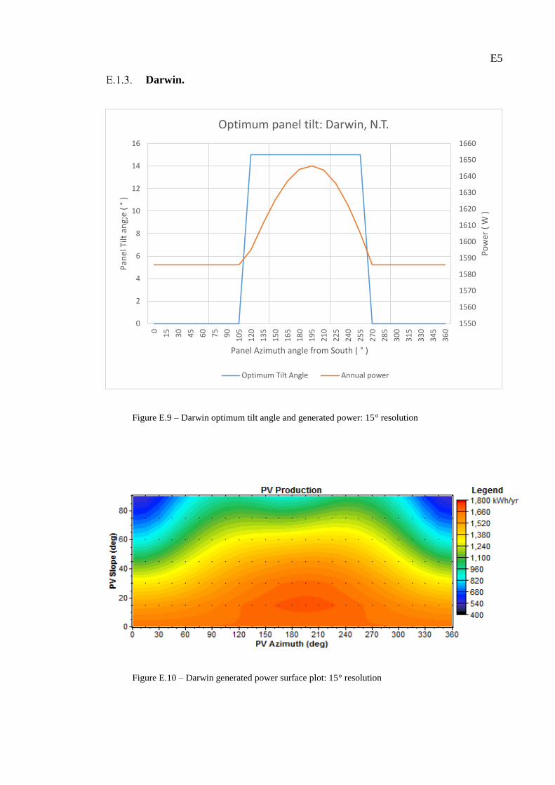
E5
Darwin.
Figure E.9 – Darwin optimum tilt angle and generated power: 15° resolution
Figure E.10 – Darwin generated power surface plot: 15° resolution
1550
1560
1570
1580
1590
1600
1610
1620
1630
1640
1650
1660
0
2
4
6
8
10
12
14
160
15
30
45
60
75
90
10
5
12
0
13
5
15
0
16
5
18
0
19
5
21
0
22
5
24
0
25
5
27
0
28
5
30
0
31
5
33
0
34
5
36
0
Po
wer
( W
)
Pan
el T
ilt a
ng;
e (
°)
Panel Azimuth angle from South ( ° )
Optimum panel tilt: Darwin, N.T.
Optimum Tilt Angle Annual power
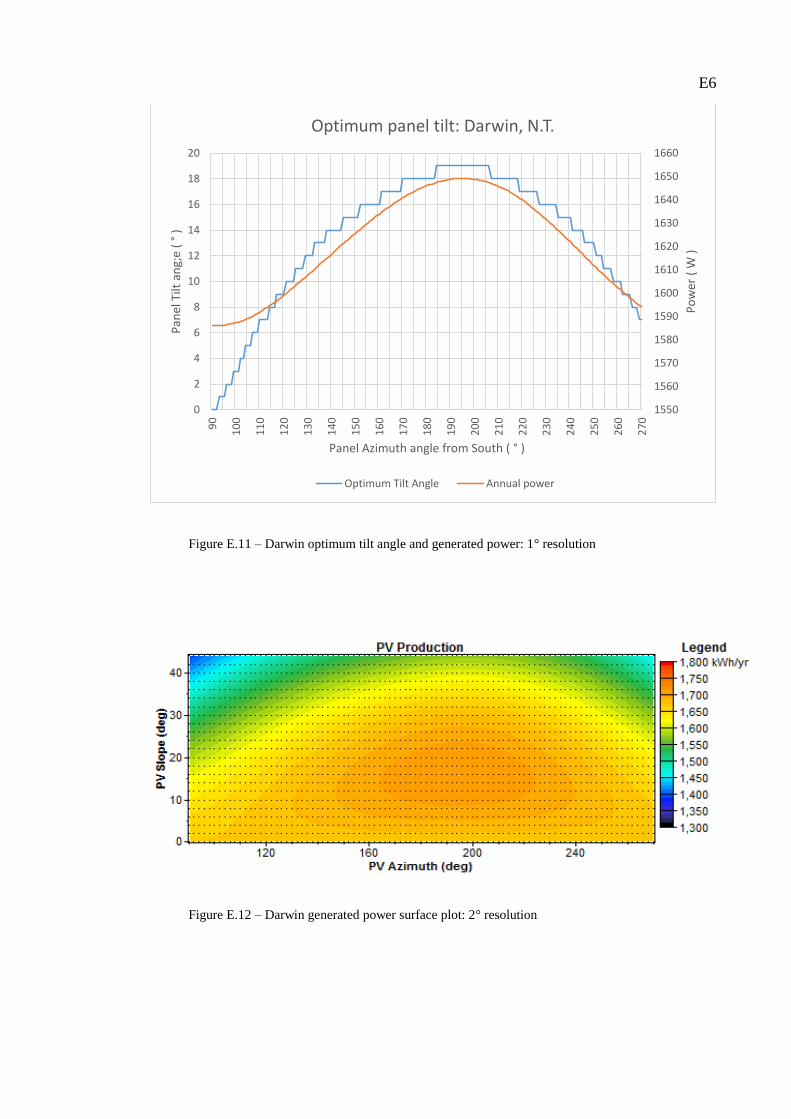
E6
Figure E.11 – Darwin optimum tilt angle and generated power: 1° resolution
Figure E.12 – Darwin generated power surface plot: 2° resolution
1550
1560
1570
1580
1590
1600
1610
1620
1630
1640
1650
1660
0
2
4
6
8
10
12
14
16
18
20
90
10
0
11
0
12
0
13
0
14
0
15
0
16
0
17
0
18
0
19
0
20
0
21
0
22
0
23
0
24
0
25
0
26
0
27
0
Po
wer
( W
)
Pan
el T
ilt a
ng;
e (
°)
Panel Azimuth angle from South ( ° )
Optimum panel tilt: Darwin, N.T.
Optimum Tilt Angle Annual power
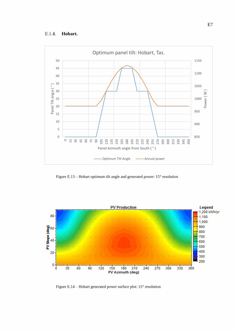
E7
Hobart.
Figure E.13 – Hobart optimum tilt angle and generated power: 15° resolution
Figure E.14 – Hobart generated power surface plot: 15° resolution
850
900
950
1000
1050
1100
1150
0
5
10
15
20
25
30
35
40
45
500
15
30
45
60
75
90
10
5
12
0
13
5
15
0
16
5
18
0
19
5
21
0
22
5
24
0
25
5
27
0
28
5
30
0
31
5
33
0
34
5
36
0
Po
wer
( W
)
Pan
el T
ilt a
ng;
e (
°)
Panel Azimuth angle from South ( ° )
Optimum panel tilt: Hobart, Tas.
Optimum Tilt Angle Annual power
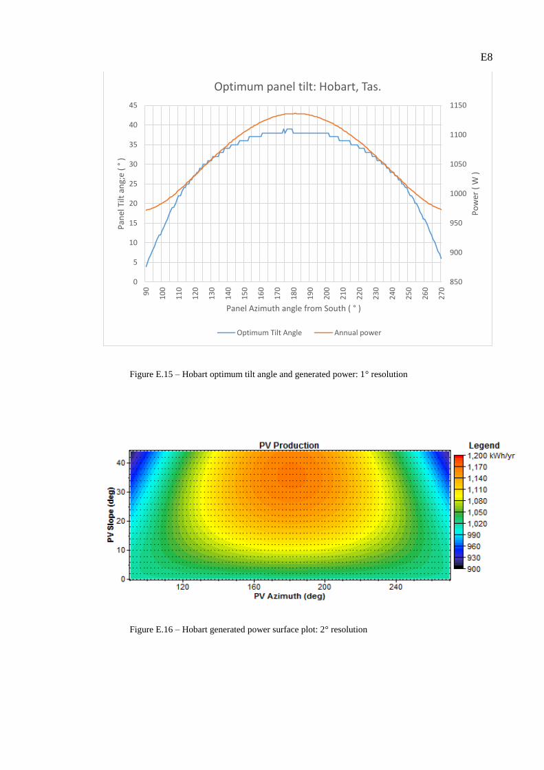
E8
Figure E.15 – Hobart optimum tilt angle and generated power: 1° resolution
Figure E.16 – Hobart generated power surface plot: 2° resolution
850
900
950
1000
1050
1100
1150
0
5
10
15
20
25
30
35
40
45
90
10
0
11
0
12
0
13
0
14
0
15
0
16
0
17
0
18
0
19
0
20
0
21
0
22
0
23
0
24
0
25
0
26
0
27
0
Po
wer
( W
)
Pan
el T
ilt a
ng;
e (
°)
Panel Azimuth angle from South ( ° )
Optimum panel tilt: Hobart, Tas.
Optimum Tilt Angle Annual power
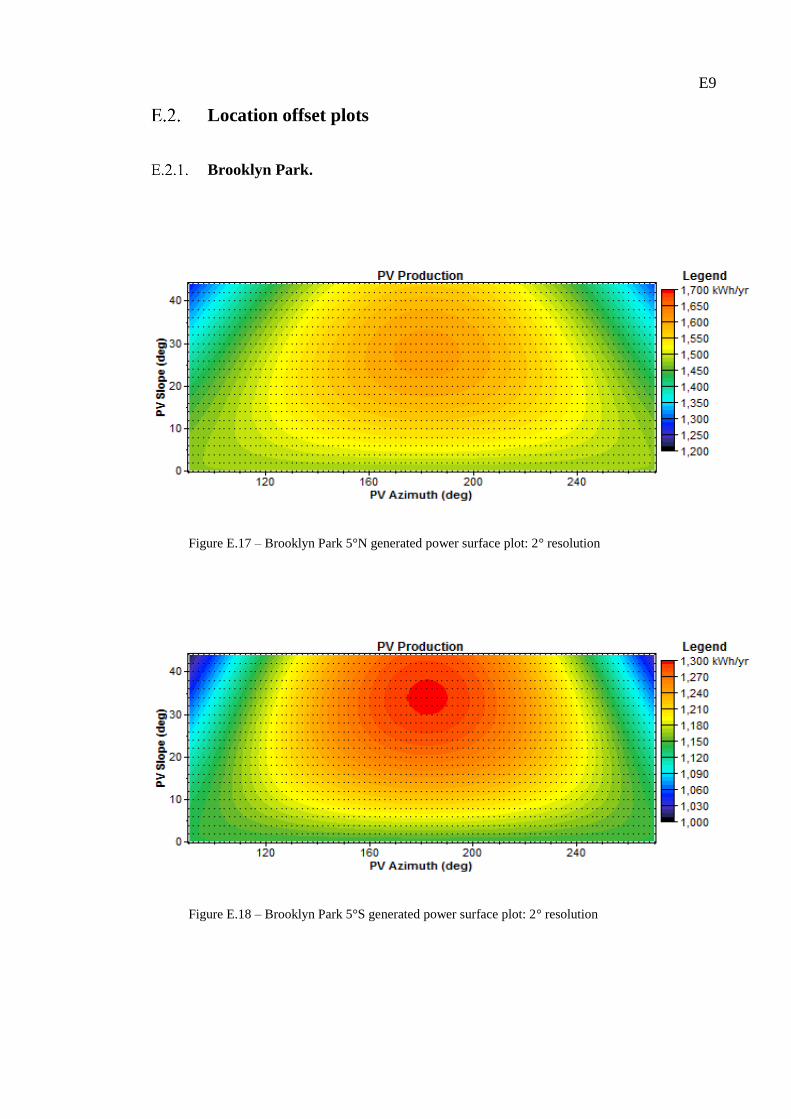
E9
Location offset plots
Brooklyn Park.
Figure E.17 – Brooklyn Park 5°N generated power surface plot: 2° resolution
Figure E.18 – Brooklyn Park 5°S generated power surface plot: 2° resolution
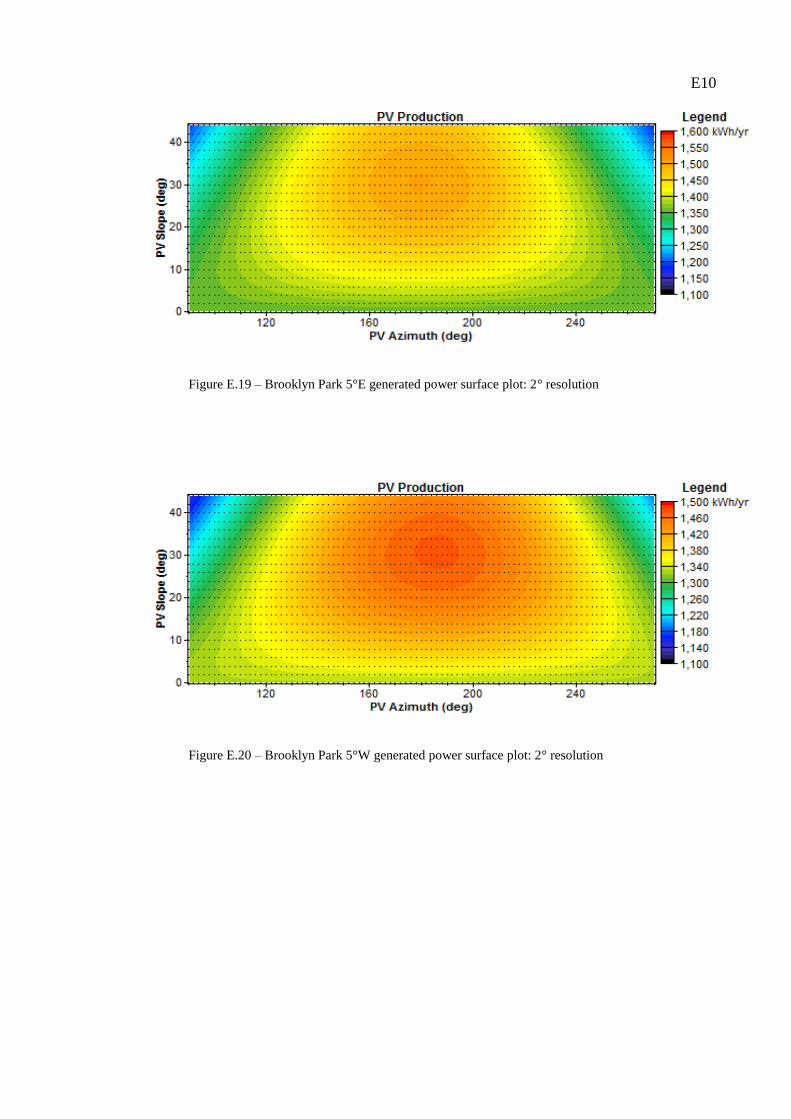
E10
Figure E.19 – Brooklyn Park 5°E generated power surface plot: 2° resolution
Figure E.20 – Brooklyn Park 5°W generated power surface plot: 2° resolution
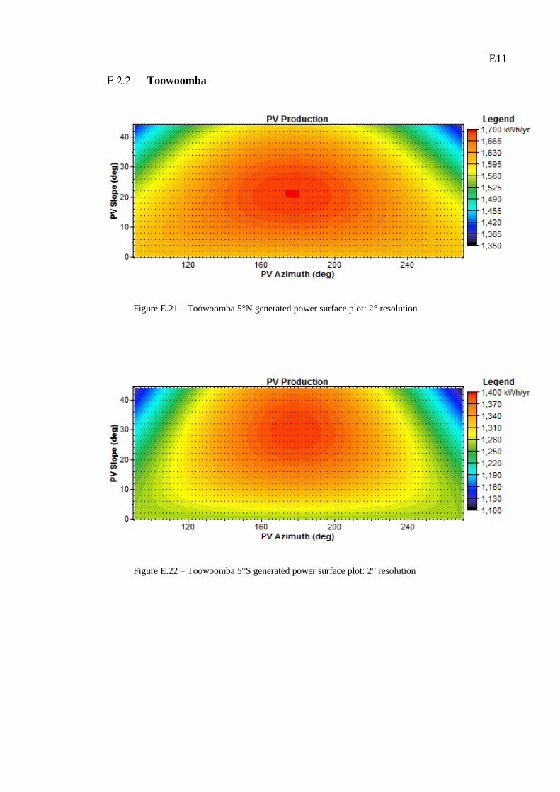
E11
Toowoomba
Figure E.21 – Toowoomba 5°N generated power surface plot: 2° resolution
Figure E.22 – Toowoomba 5°S generated power surface plot: 2° resolution
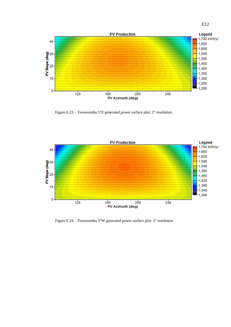
E12
Figure E.23 – Toowoomba 5°E generated power surface plot: 2° resolution
Figure E.24 – Toowoomba 5°W generated power surface plot: 2° resolution
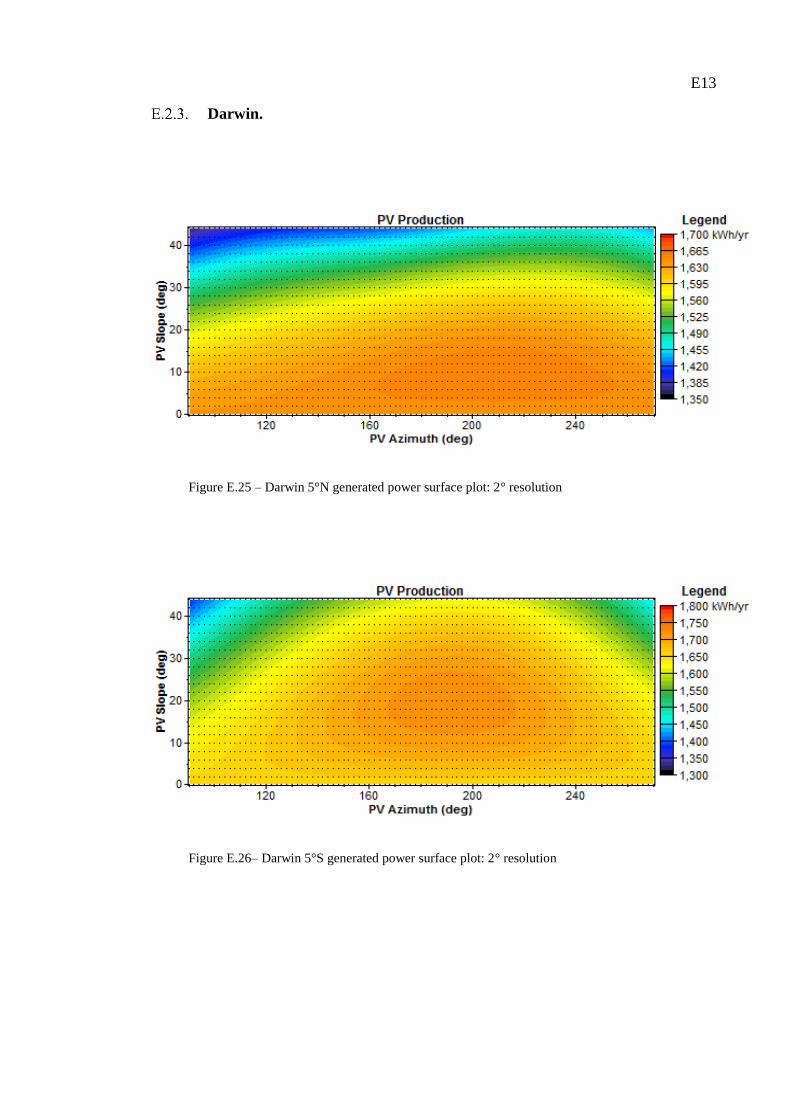
E13
Darwin.
Figure E.25 – Darwin 5°N generated power surface plot: 2° resolution
Figure E.26– Darwin 5°S generated power surface plot: 2° resolution
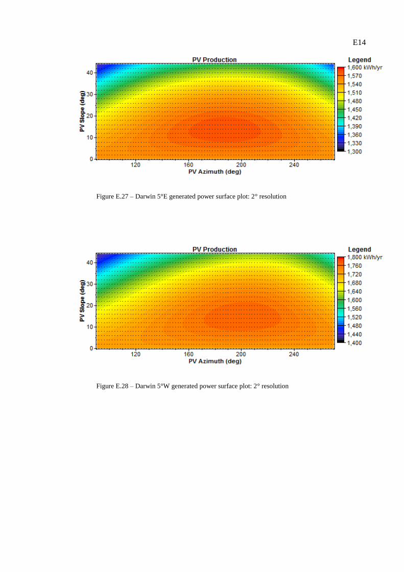
E14
Figure E.27 – Darwin 5°E generated power surface plot: 2° resolution
Figure E.28 – Darwin 5°W generated power surface plot: 2° resolution
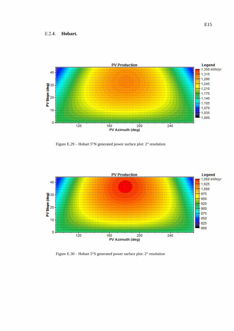
E15
Hobart.
Figure E.29 – Hobart 5°N generated power surface plot: 2° resolution
Figure E.30 – Hobart 5°S generated power surface plot: 2° resolution
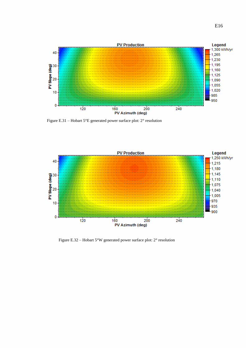
E16
Figure E.31 – Hobart 5°E generated power surface plot: 2° resolution
Figure E.32 – Hobart 5°W generated power surface plot: 2° resolution

Hazard identification and risk assessments

F1
Hazard identification.
Solar installations
Is there adequate information relating to,
o Existing electrical installation,
o Existing solar installation. (Applicable to site with existing solar system
only)
Does the following exist,
o Safe working procedure,
o Installers certified to work at heights,
o Installer licensed to perform work on mains electrical installation,
o Installer licensed to install solar systems.
Have the following factors been considered during this risk assessment,
o Input from installation workers,
o Work related stress factors,
o Requirements of different worker groups,
o Requirement for PPE.
Can risk be minimised by the following,
o Isolating power prior to connection to mains,
o Avoid working alone.
Is there a risk of injury or illness due to the following,
o Falling from heights,
o Slipping or falling on unsuitable working surface,
o Slipping or falling due to holes of skylights,
o Suitability of ladder to assess working surface,
o Tools or equipment being dropped from heights,
o Lifting heavy items,
o Water present around electrical work,
o Failure to maintain minimum electrical clearance from HV power lines,
o Electrical hazard from PV generated power,
o Repetitive work process,
o Prolonged kneeling or squatting.
Any other items which have not been covered.

F2
Project.
Has the following been considered throughout this hazard identification.
o Work related stress factors,
o Risk of data loss
Is there a risk of injury or illness due to the following,
o Eye strain,
o Repetitive movements,
o Adequate lighting on the work surface,
o Sitting for extended period of time,
o Any other items which have not been covered.
(European Agency for Safety and Health at Work, n.d.)
Risk matrix scores.
The relative priority of each identified item within the risk assessment is determined using
a numerical scoring process. Values for this process are detailed in table F.1, and overall
risk level is detailed in table F.2. (University of Melbourne, 2004)
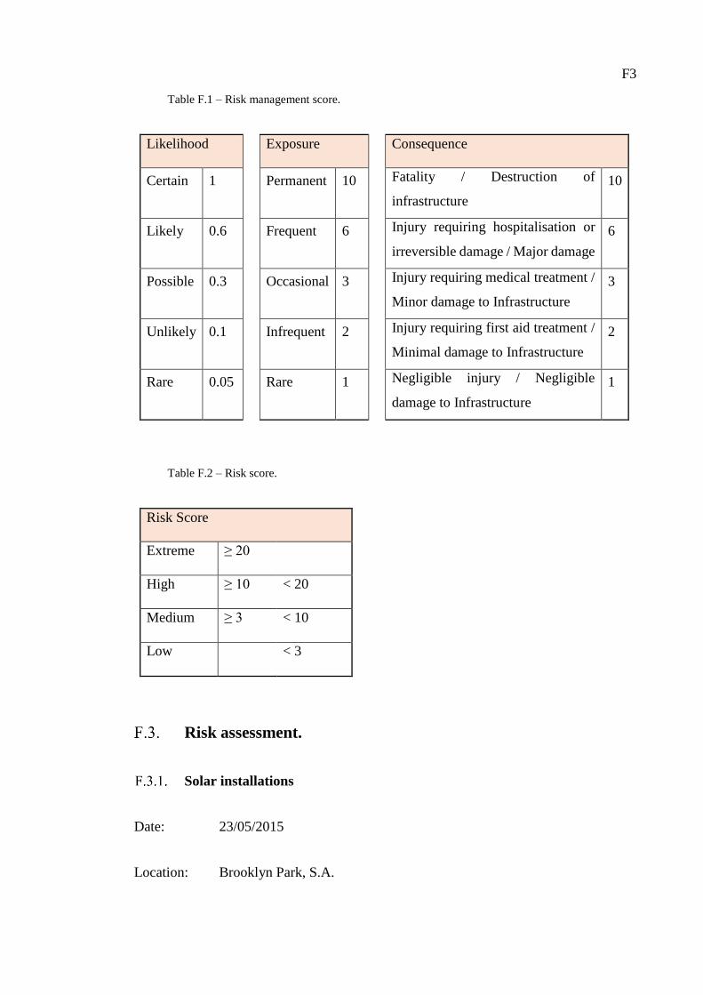
F3
Table F.1 – Risk management score.
Likelihood Exposure Consequence
Certain 1 Permanent 10 Fatality / Destruction of
infrastructure
10
Likely 0.6 Frequent 6 Injury requiring hospitalisation or
irreversible damage / Major damage
to Infrastructure
6
Possible 0.3 Occasional 3 Injury requiring medical treatment /
Minor damage to Infrastructure
3
Unlikely 0.1 Infrequent 2 Injury requiring first aid treatment /
Minimal damage to Infrastructure
2
Rare 0.05 Rare 1 Negligible injury / Negligible
damage to Infrastructure
1
Table F.2 – Risk score.
Risk Score
Extreme ≥ 20
High ≥ 10 < 20
Medium ≥ 3 < 10
Low < 3
Risk assessment.
Solar installations
Date: 23/05/2015
Location: Brooklyn Park, S.A.
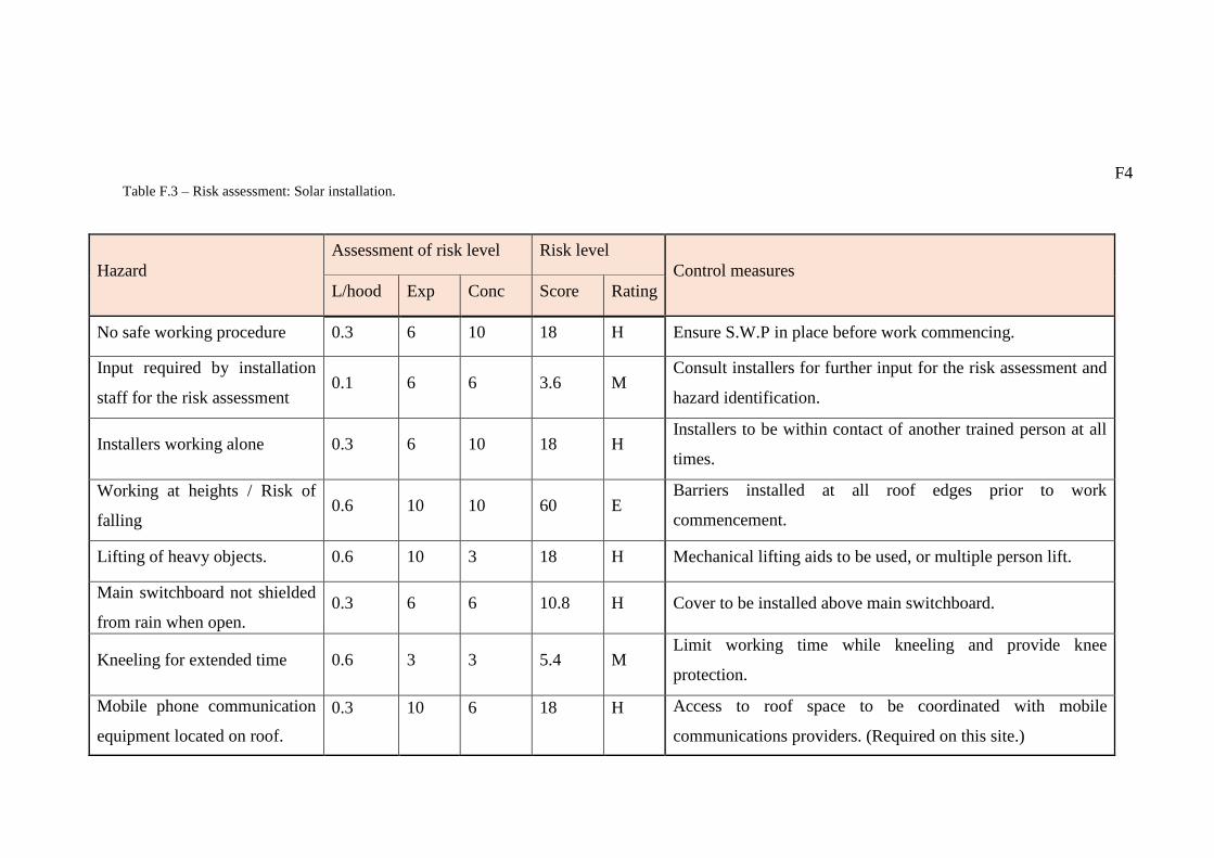
F4 Table F.3 – Risk assessment: Solar installation.
Hazard
Assessment of risk level Risk level
Control measures
L/hood Exp Conc Score Rating
No safe working procedure 0.3 6 10 18 H Ensure S.W.P in place before work commencing.
Input required by installation
staff for the risk assessment 0.1 6 6 3.6 M
Consult installers for further input for the risk assessment and
hazard identification.
Installers working alone 0.3 6 10 18 H Installers to be within contact of another trained person at all
times.
Working at heights / Risk of
falling 0.6 10 10 60 E
Barriers installed at all roof edges prior to work
commencement.
Safety harnesses to be used if barriers are not feasible. Lifting of heavy objects. 0.6 10 3 18 H Mechanical lifting aids to be used, or multiple person lift.
Main switchboard not shielded
from rain when open. 0.3 6 6 10.8 H Cover to be installed above main switchboard.
Kneeling for extended time 0.6 3 3 5.4 M Limit working time while kneeling and provide knee
protection.
Mobile phone communication
equipment located on roof.
0.3 10 6 18 H Access to roof space to be coordinated with mobile
communications providers. (Required on this site.)
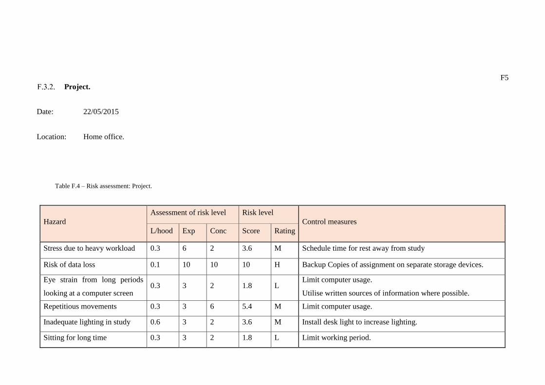
F5
Project.
Date: 22/05/2015
Location: Home office.
Table F.4 – Risk assessment: Project.
Hazard
Assessment of risk level Risk level
Control measures
L/hood Exp Conc Score Rating
Stress due to heavy workload 0.3 6 2 3.6 M Schedule time for rest away from study
Risk of data loss 0.1 10 10 10 H Backup Copies of assignment on separate storage devices.
Eye strain from long periods
looking at a computer screen 0.3 3 2 1.8 L
Limit computer usage.
Utilise written sources of information where possible.
Repetitious movements 0.3 3 6 5.4 M Limit computer usage.
Inadequate lighting in study 0.6 3 2 3.6 M Install desk light to increase lighting.
Sitting for long time 0.3 3 2 1.8 L Limit working period.

Specification sheets
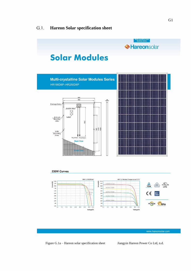
G1
Hareon Solar specification sheet
Figure G.1a – Hareon solar specification sheet Jiangyin Hareon Power Co Ltd, n.d.
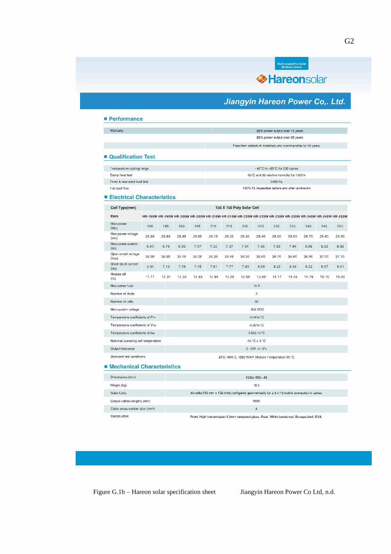
G2
Figure G.1b – Hareon solar specification sheet Jiangyin Hareon Power Co Ltd, n.d.

G3
Tindo Solar specification sheet
Figure G.2a – Tindo solar specification sheet Tindo Solar, 2015
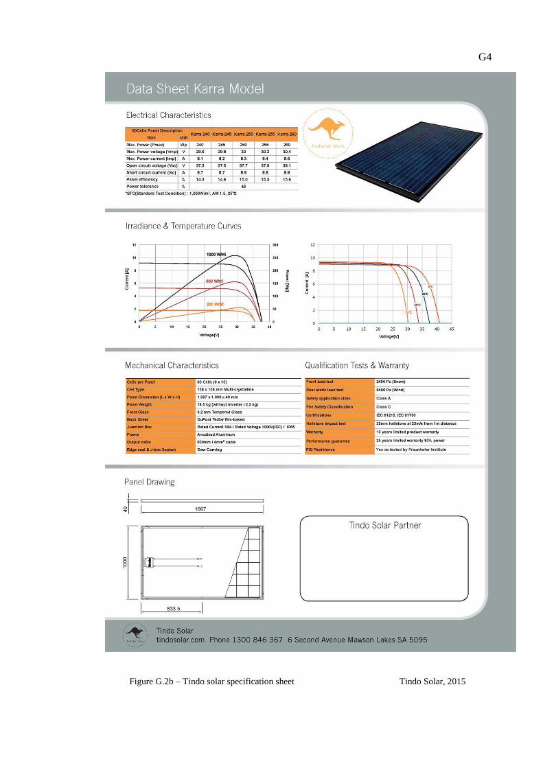
G4
Figure G.2b – Tindo solar specification sheet Tindo Solar, 2015