0

University of São Paulo

“Luiz de Queiroz” College of Agriculture

Quantitative parameterization of soil surface structure with increasing

rainfall volumes

Edison Aparecido Mome Filho

Thesis presented to obtain the degree of Doctor in

Science. Area: Soil and Plant Nutrition

Piracicaba

2016

1

Edison Aparecido Mome Filho

Agronomist

Quantitative parameterization of soil surface structure with increasing rainfall volumes versão revisada de acordo com a resolução CoPGr 6018 de 2011

Advisor:

Prof. Dr. MIGUEL COOPER

Thesis presented to obtain the degree of Doctor in

Science. Area: Soil and Plant Nutrition

Piracicaba

2016

Dados Internacionais de Catalogação na Publicação

DIVISÃO DE BIBLIOTECA - DIBD/ESALQ/USP

Mome Filho, Edison Aparecido Quantitative parameterization of soil surface structure with increasing rainfall volumes /

Edison Aparecido Mome Filho. - - versão revisada de acordo com a resolução CoPGr 6018 de 2011. - - Piracicaba, 2016.

94 p. : il.

Tese (Doutorado) - - Escola Superior de Agricultura “Luiz de Queiroz”.

1. Erosão pela água 2. Microrelevo 3. Escala 4. Sistema poroso I. Título

CDD 631.45 M732q

“Permitida a cópia total ou parcial deste documento, desde que citada a fonte – O autor”

3

DEDICATE

To my parents,

Edison and Izabel,

for all their believe and support, since my early years.

“Barulho de trovoada, coriscos em profusão

A chuva caindo em cascata, na terra fofa do chão

Virando em lama a poeira, poeira vermelha

Poeira, poeira do meu sertão

Poeira entra meus olhos, não fico zangado não

Pois sei que quando eu morrer, meu corpo irá para o chão

Se transformar em poeira, poeira vermelha...”

music by

Luiz Bonan and Serafim C. Gomes

4

5

AKNOWLEDGEMENTS

After 4 years, I believe that the most difficult part was not to discuss my dataset, but

trying to remember all the people that helped me along the way. Therefore, I ask in advance,

please forgive me if your name is not cited in these next lines. Nevertheless, if you did

anything, does not matter how small it was, to help me achieve the results exposed in this text,

know that I own you a life debt, even if I do not remember it.

First of all, I want to thank FAPESP for the scholarships, under processes 2013/08736-

6 and 2014/05738-0, that allowed this project to become true.

Secondly, but not less, I would like to thank my family, my parents, Edison and Izabel,

my brother and sister, Ricardo and Erica, my sister in law, Maria, as well as my nephew and

niece, Giacomo and Isabel, for soften my life during such hard years.

To “older” friends of the Soil Science department, Osvaldo, Sueli, Sâmala, Getúlio,

Lorena, Raul, Renata Beltz, Selene, Mariana and Laura, I thank the hours of discussion,

where you were patient enough to hear much more than speak.

To “newer” friends, Hélio, Renato, Sara and Raquel, thanks for all the coffee hours.

To the whole class of 2005 from the best Unesp campus in the world, thank you for

being part of my early career years, that prepared me for this moment. Special thanks to

Rufião and Salsicha, whom made my time in Piracicaba to look like it was just a continuation

of my undergrad period.

Thanks to Erreinaldo and everybody at the LPV for allowing me to use their area for

my experimentation, and for giving me support every time that I needed.

Thanks to all the interns that helped me in all steps of my field and lab work: Julia,

Katharina, Patrick, Marte, Felipe and Vitor.

Thanks to Dr. Alvaro Pires da Silva for letting me use his lab facilities, and to his crew,

Jair and Rossi, that helped me during part of my analysis.

Thanks to Sonia and Chiquinho for all the good work in the manufacturing of excellent

impregnated soil blocks, and for helping me at the lab whenever you could.

Thanks to Dr. Daniel Gimenez and Dr. Richard Heck, for all the learning and support

during my time in foreign lands.

Thanks to Eliana for correcting this text, and everybody that work at the library from

the College of Agriculture, for all the help during my master’s and doctorate.

6

We are coming to an end. Again, hope your name was cited here, if not, know that only

four names are in my mind now. I know what you are thinking - “you ungrateful b…!”. Well,

get over it and let us continue.

First, I would like to thank Virginia and Gonzalo for all the good moments. But

especial thanks must be given to Virginia. If you can see 12 beautiful and long tables along

this text, filled with the most interesting data about surface sealing and all that science stuff, is

because she organized those tables. I have to say, is not every day that you have an intern with

a Master degree working for you.

Secondly, I would like to thank Rodrigo Zenero. Without your work, there would be no

thesis. Normally, we do not read about problems in the final work. However, I must declare

that, if in this world, demons and evil creatures are real, part of them must live inside

electrical devices. And a half of the population live inside our “dear” MicroRelief Meter. You

should be canonized for being able to make it finish my readings when I most needed it.

Thirdly, thanks to my advisor, Dr. Miguel Cooper. After four years, you have learned

how stubborn I can be. And, even so, during all this time you gave me your support and

advise. I cannot say that I changed, but I sure have matured during the time working with you.

Hope to continue our partnership in the years to come.

And last, but not least. During the last years I am getting more and more certain that

there is no supreme being in the middle of the universe controlling our lives. No master in the

universe. No after, just now. However, I cannot deny the faith of my parents, that, by holding

them up, it kept me strait on my path. At the same time, a dear friend of mine, already thanked

previously, gave me good moments of discussion about God, life and its mysteries, during

this last semester. The overall lesson that I take from it all, is that we born, live, and die,

without knowing nothing for sure. Doubt, as logic, is the very essence of the human race. So,

if I do not even know it for sure if multifractal parameters do really mean something, whom

am I to deny the existence of something? Thus, in the name of my parents, I thank their God,

who, by making them happier in some way, made me a blessed man.

7

SUMMARY

RTESUMO…………………………………………………………………………… 9

ABSTRACT…………………………………………………………………………... 11

1 INTRODUCTION…………………………………………………………………. 13

2 DEVELOPMENT…………………………………………………………………... 15

2.1 Literature review………………………………………………………………….. 15

2.1.1 Analyses of complex systems: soil as a multifractal…………………………… 15

2.1.1.1 Fractal theory…………………………………………………………………. 15

2.1.1.2 Fractals in Nature……………………………………………………………... 16

2.1.1.3 Multifractal theory……………………………………………………………. 18

2.1.1.3.1 Legendre transformation of τ(q)……………………………………………. 19

2.1.1.3.2 Partition function ………………………………………………... 20

2.1.1.3.3 Multifractal spectrum parameters………………………………………..... 21

2.1.1.4 Fractal and multifractal applications in soil science…………………………. 23

2.1.2 Definition of soil physical quality – stability and functioning…………………. 24

2.1.3 Soil erosion: its mechanic and the “sealing” process…………………………... 26

2.1.3.1 Physical Erosion……………………………………………………………… 26

2.1.3.1.1 Mechanics of erosion caused by rainfall……………………………………. 27

2.1.3.1.1.1 Rainfall erosivity and soil erodibility…………………………………….. 27

2.1.3.1.1.2 Particles and aggregates detachment and transport……………………… 28

2.1.3.1.1.3 Particles and aggregates deposition – sealing and crust formation………. 28

2.1.4 Soil surface roughness vs soil physical quality…………………………………. 30

2.1.5 Soil structure image analysis …………………………………………………... 31

2.2 Material and methods……………………………………………………………. 32

2.2.2 Soil preparation and experimental design……………………………………... 33

2.2.3 Rainfall simulation…………………………………………………………….. 36

2.2.4 Soil surface roughness measurements………………………………………… 37

2.2.5 Soil attributes………………………………………………………………….. 37

2.2.5.1 Chemical analyses…………………………………………………………… 37

2.2.5.2 Physical analyses……………………………………………………………. 38

2.2.5.3 Hydrological analyses……………………………………………………….. 39

2.2.6 Image analyses………………………………………………………………… 40

8

2.2.6.1 Micromorphometrical analyses……………………………………………… 40

2.2.6.2 Soil surface roughness analyses……………………………………………... 42

2.2.6.3 Multifractal analysis………………………………………………………… 43

2.2.7 Statistical analyses…………………………………………………………….. 44

2.3 Results and discussion…………………………………………………………... 45

2.3.1 Soil surface roughness………………………………………………………… 45

2.3.1.1 Random Roughness - RRi…………………………………………………… 49

2.3.1.2 Multifractal analyses of the soil surface roughness…………………………. 50

2.3.2 Physical attributes……………………………………………………………... 56

2.3.2.1 Bulk Density and Ratio of Volume of Pores………………………………… 56

2.3.2.2 Aggregates stability…………………………………………………………. 57

2.3.3 Hydrological attributes………………………………………………………... 60

2.3.3.1 Unsaturated soil hydraulic conductivity - K(θ)……………………………... 60

2.3.3.2 Water Retention Curve – WRC……………………………………………... 60

2.3.4 Image Pore Analysis…………………………………………………………... 64

2.3.4.1 Micromorphometrical analysis……………………………………………… 64

2.3.4.2 Multifractal analyses of pores……………………………………………….. 74

3 CONCLUSIONS………………………………………………………………….. 79

REFERENCES……………………………………………………………………… 81

9

RESUMO

Parametrização quantitativa da estrutura da superfície do solo em volumes crescentes

de chuva

O estudo da estrutura do solo permite inferências sobre seu comportamento. Parâmetros

quantitativos são comumente utilizados na avaliação da estrutura e os multifractais ainda são

subutilizados na ciência do solo. Alguns estudos mostraram relação entre parâmetros

multifractais com a diminuição da rugosidade superficial do solo devido à chuva e a

heterogeneidade do sistema poroso. No entanto, uma assinatura multifractal relacionada a um

comportamento específico do solo ainda não está estabelecida. Portanto, os objetivos desta

pesquisa foram: (i) relacionar parâmetros multifractais com mudanças na estrutura do solo por

meio da análise de mapas de rugosidade superficial e de imagens 2D provenientes de blocos

impregnados de solo; e (ii) utilizar estes parâmetros para identificar as etapas de degradação

do solo devido ao selamento e encrostamento superficial. Um experimento com chuva

simulada com intensidade de 120 mm h-1

foi montado em uma Nitossolo Vermelho

eutroférrico argiloso em parcelas quadruplas onde aplicou-se volumes de 40, 80 e 120 mm,

mais um controle sem-chuva. A evolução da rugosidade superficial foi avaliada em três

escalas: um rugosímetro de campo (MRM) reuniu leituras numa grade fixa (10 x 10 mm,

640000 mm²); um escâner com triangulação de lasers em multilinhas (MLT) foi usado em

laboratório, sobre blocos de solo, criando uma grade aleatório (0,5 mm de resolução, 5625

mm²); um tomógrafo de raios-X (XRT) reuniu leituras de um bloco de solo em uma grade fixa

(0,074 x 0,074 mm, de 900 mm²). Para a análise micromorfométrica, amostras de solo

indeformado (0,12 x 0,07 x 0,05 m) foram impregnadas, cortadas em blocos, polidas e

subdivididas em três camadas (0 a 10 mm, 20 a 30 mm e de 40 a 50 mm), paralelas à

superfície, tendo cinco imagens (ampliação de 10x, 156,25 µm2 pixel

-1) geradas por camada.

Após a segmentação, três imagens foram selecionadas por camada e o sistema poroso foi

avaliado. Análises de rugosidade não mostraram diferenças (p > 0.10) entre parâmetros

multifractais nas medições da escala MRM, enquanto MLT e XRT puderam ser utilizadas

para modelar a degradação da rugosidade com o aumento do volume de chuva. Como essas

duas ultimas escalas apresentaram resultados similares, MLT poderia substituir o uso de XRT

em tais análises, devido ao seu menor custo e possibilidade de cobrir área mais vasta durante

as análises. O comportamento multifractal dos poros mudou de acordo com o

desenvolvimento do selamento superficial e da camada avaliada, sendo sensitivo a mudanças

no grau de fragmentação (número de poros) dentro de cada classe de tamanho de poros. As

dimensões de Hausdorff a esquerda do espectro (Lf(α)min, LΔf(α) and D2) tiveram relação

linear com o aumento de volume de chuva para ambas medições de rugosidade superficial do

solo e de área de poros. Entretanto, D2 não foi significativo (p > 0.10) entre volumes de chuva

para diferenciar a porosidade próxima a superfície, embora os parâmetros D0-D1, D0-D2 e

D1-D2 pudessem ser utilizados para descrever mudanças nessa camada. Conclui-se que o

espectro multifractal é sensível à mudanças estruturais no solo causadas pela chuva e que

pode ser utilizado na parametrização da degradação da rugosidade superficial do solo e da

porosidade.

Palavras-chave: Erosão pela água; Microrelevo; Escala; Sistema poroso

10

11

ABSTRACT

Quantitative parameterization of soil surface structure with increasing rainfall volumes

The study of soil structure allows inferences on soil behavior. Quantitative parameters

are oftentimes required to describe soil structure and the multifractal ones are still underused

in soil science. Some studies have shown relations between the multifractal spectrum and both

soil surface roughness decay by rainfall and porous system heterogeneity, however, a

particular multifractal response to a specific soil behavior is not established yet. Therefore, the

objectives of this research were: (i) to establish relations between multifractal parameters and

soil structure changes by analyzing both soil surface roughness maps and 2D images from

impregnated soil blocks; and (ii) to utilize these parameters to evaluate soil surface

degradation by the processes of crusting and sealing. An experiment with simulated rainfall

was assembled on a Fine Rhodic Kandiudalf with an intensity of 120 mm h-1

in quadruplicate

plots at amounts of 40, 80, and 120 mm, plus a no-rainfall control. The evolution of the

surface roughness was evaluated in three scales of measurement: a field microrelief meter

(MRM) gathered readings on a fixed grid (10 x 10 mm, 640,000 mm²); a multistripe laser

triangulation (MLT) scanner was used in the laboratory in soil blocks, creating a random

mesh (0.5 mm of resolution, 5625 mm²); an X-ray tomography (XRT) scanner gathered

readings of a soil block on a fixed grid (0.074 x 0.074 mm, 900 mm²). For

micromorphometrical analysis, undisturbed soil samples (0.12 x 0.07 x 0.05 m) were

impregnated, sliced in blocks and polished. Each block was divided into three layers (0 to 10

mm, 20 to 30 mm and 40 to 50 mm), parallel to surface, and five images (10X magnification,

156.25 µm2 pixel

-1) were taken by layer. After segmentation, three representative images were

chosen by layer and the pore system was evaluated. Roughness analyzes showed no

differences (p > 0.10) between multifractal parameters across rainfall amounts for MRM

measurements, while both MLT and XRT could be used to model roughness degradation by

rainfall increase. Since the last two scales presented similar results, MLT could replace XRT

in such analysis, due to its lower cost and possibility of a larger area coverage. The

multifractal behavior of pores changed according to sealing development and depth of

measurement, being sensitive to the changes on size distribution and fragmentation degree

(number of pores) within each size class. The Hausdorff dimensions at the left side of the

spectrum (Lf(α)min, LΔf(α) and D2) showed a linear behavior with increasing rainfall amount,

considering both soil surface roughness and area of pores measurements. However, D2 was

not different (p > 0.10) along rainfalls for the porosity closer to surface, although parameters

D0-D1, D0-D2 and D1-D2 could be used to described the changes in this layer. Was

concluded that the multifractal spectrum is sensitive to structure changes caused by rainfall

and that it can be used to parameterize both soil surface and pores degradation.

Keywords: Water erosiom; Microtopography; Scale; Porous system

12

13

1 INTRODUCTION

The description of the soil structure assists the understanding of its behavior in the

environment, which is important to explain complex processes that occur in the soil, such as

water and air movement, nutrient cycling and erosion. However, characterization of the

structure must not depend only on its visual description if we want to logically describe the

system. Particularly, to understand a physical process, a mathematical approach is very often

the most appropriate, because it uses a logical organization of thoughts to explain the system.

As a result, soil physicists rely on both mathematical and statistical modeling to describe

processes in soil, and a range of indexes are used to characterize physical quality of a soil.

In the last century, several methods were used to estimate numerical data, which were

used to express soil structure regarding its stability and functioning. These methods are

mainly based on direct measurements of one or more soil physical attributes that, after some

mathematical reasoning are linked to a determined behavior. For instance, aggregates size

distribution can be used to calculate the weighted mean diameter, which is commonly used to

describe the stability of the soil structure. On the other side both pores size and shape

distribution are associated to several flux equations and used to model both inputs and outputs

in soil, which basically governs soil functioning. The association between stability and

functioning dictates the physical quality of a soil, that may be addressed in different ways. For

example, to achieve high crop productivity, the ideal relation between stability and

functioning may not be the same as to the one to reduce erosion rates to a minimum.

Therefore, the term soil physical quality can be ambiguous. This subject will be developed

during the section 2.1.2 to clarify the objectives and the methodology used during this

research.

Nonetheless, since soil presents several functions on the ecosystem, which may lead to a

range of indexes used to characterize it, it may be considered as a complex system. This

brings up the importance of finding a parameter that relates to several soil attributes, allowing

its interpretation in several areas of research. The fractal theory was broadly employed in the

study of chaotic systems, such as turbulence, and in soil science it was used as a parameter to

describe patterns of spatial distribution of different materials, from fungi and bacterial

communities until scaling properties of soil aggregation, that interferes in both pores size and

shape distribution. However, the range of interpretations that can be uniquely drawn from

fractal results is very narrow. The main issue with interpretations only based in a fractal

approach is to rely on a unique number so that it will describe several processes occurring at

the same time. Thus, the fractal dimension of a dataset is often correlated to other variables

14

before conclusions can be made. In that sense, the multifractal approach allows more

flexibility, as it will be scrutinized throughout this text, and a range of interpretations can be

made without the need of other variables input. However, its use is still incipient in soil

science. This fact may be associated to the multiplicity of parameters displayed by such

analysis, many of whom still lack physical interpretation.

Therefore, the objectives of this research were: (i) to establish relations between

multifractal parameters and soil structure changes by analyzing both soil surface roughness

maps and 2D images from impregnated soil blocks; and (ii) to utilize these parameters to

evaluate soil surface degradation by the processes of crusting and sealing.

The hypothesis tested were: i) The multifractal spectra is sensitive to structure changes

caused by a range of rainfall amounts; ii) some multifractal parameters can be used to model

the steps of soil surface degradation by rainfall.

15

2 DEVELOPMENT

2.1 Literature review

2.1.1 Analyses of complex systems: soil as a multifractal

A complex system is one that presents a challenge against universal modeling. In other

words, when it is difficult to find a suitable model to describe phenomena, because these

occur in a system that has too many variables, we call this system complex (CHU, 2011). The

fractal theory has aided the understanding of several complex systems where other

mathematical approaches have shown to be laborious, or even erroneous. Because of that, a

quick review of this theory is provided.

2.1.1.1 Fractal theory

In Mathematics, the dimension of a space can be described as the minimum set of

coordinates to specify any points within it. The theory of measure, by Henri Labesgue, gives

the notion of linear measure on a straight line, of plane measure on a bi-dimensional plane, of

volume measure in three dimensional space (BESICOVITCH, 1928). Knowing that length

exists not only in straight lines, but also in a space, Constantin Carathéodory defined the s-

dimension of a set in a q-dimensional space as any integer number considering q s. This

states the dimensions in a Euclidean space, which are always integer numbers

(BESICOVITCH, 1928).

With the development of the set theory and Georg Cantor’s idea of the existence of

uncountable sets (an infinite of infinities), the Euclidean point of view, traced by general

topology, changed and mathematicians proved the possibility of non-integer dimensions.

Hausdorff (1919) using the axiomatic of set theory wrote a paper on his definitions of

dimensions, and Besicovitch (1928, 1937) applied Hausdorff theorems on the description of

sets of fractional dimensions. The definition is as follows, and can be similarly applied to

higher dimensional spaces: considering a finite sequence of sets Ui (U1,U2,…,Un) that cover a

set A (Ui A) in a q-dimensional space (q equals a positive integer), and knowing di is the

sequence (d1, d2,…, dn) of the diameters of Ui, which di δ, and δ is a positive number, the s-

dimension of the measure A (s-dimA) can be defined as:

(1)

In a linear set Besicovitch assumed three possibilities: (i) there exists 0 1, if

for and for , then A is a s-dimensional set; (ii)

if for any , then A is one-dimensional; (ii) if for any

16

, then A is 0-dimensional. This was called the Hausdorff dimension of a set and, due to

the possibility of fractional dimensions, was useful to describe the geometry of some strange

sets.

To compute the dimension of an object is easier to calculate the Minkowski-Bouligand

dimension, which is, in most occasions, similar to the Hausdorff dimension. A way to

calculate this is to cover the object with boxes with different side lengths L. The relation

between L and the number of boxes N(L) that cover the object follows a power law

(2)

and, when L , the boxes approximate the real shape and size of the object,

expressing Equation 3.

(3)

D is Minkowski-Bouligand dimension, also called the box-counting dimension, and

is a proportionality constant that represents the number of initiators of the object. This

equation can also calculate the topological dimension of lines, squares and cubes, but nothing

prevents D of being a non-integer number.

If the boxes are square, there is a scale relation when L decreases and a more

insightful way of writing Equation 3 is:

(4)

Where

is the number of boxes with size

, and is the scale factor. When is

1, D can be expressed by using logarithm in Equation 5, where we can calculate D by two

forms, approximately, by the slope of the log log plot of

vs

, or exactly, by finding

the limit of this function.

(5)

2.1.1.2 Fractals in Nature

As stated before, the fractional dimension is not new in mathematics. However, its use

to explain physical phenomena started only in 1967. By measuring the coast of several

countries and continents in different scales, Richardson (1961) showed that conventional

measurement techniques could give enormously distinct results, with lengths increasing

rapidly according to the magnification of the scale. Based on plots of scale vs length,

17

Richardson saw a power law relation. Therefore, he used a log plotting to calculate the slopes

of such relations and propose to use this parameter to distinguish the coastlines.

Mandelbrot (1967) made a mathematical interpretation of Richardson’s measurements

using Equation 3 as basis, considering that the number N(d) of segments of length d needed to

walk across the coastline was proportional to (1/d)D, for some exponent D and a

proportionality constant k (Equation 6).

(6)

The length L( ) of the coastline would be equal to the sum of all d:

(7)

Therefore, by joining Equations 6 and 7:

(8)

Applying logarithms:

(9)

If the initiator is a unique line, , and because its length would depend on the

scale of measurement, may be substituted by

, where is a scale factor, generating

Equation 10:

(10)

If the data points of Richardson’s log log plots lied along a straight line, the

assumption on Equation 6 was justified, and Mandelbrot called the exponent D as the “fractal

dimension” of the coastline, permitting Richardson's data to be interpreted by this value. This

was the first proof that, at some scales, natural systems could be represented by a simple

power law that relates the characteristics of an object to an exponent, which was considered as

a dimension of the system.

Mandelbrot used the term “fractal” to designate the objects that exhibit repeating

patterns at different scales and did extensive work on reviewing, theorizing and describing

such objects and their relations with physical systems. Such interpretations were impacting in

the study of chaotic systems, since the fractal dimension helps to explain the scale relation of

complex shapes, where details appear to contain more information than the general analysis of

the object. Therefore, the fractal theory defines spatial and temporal models of systems that

18

exhibit a range of symmetry, characterized by a power law dependent on the number of

repetitions of a given characteristic.

2.1.1.3 Multifractal theory

Although the fractal theory presents an easy way of characterize a system, complex

structures of nature present variations that cannot be analyzed by a simple fractal model. In

nature most of the processes are stochastic, and the mass distribution along the systems is not

homogeneous. The multifractal analysis includes this density variation, which are expressed

in a multifractal spectrum (CHHABRA et al., 1989; CHHABRA; JENSEN, 1989) that gives a

quantitative description of a heterogeneous phenomenon (STANLEY; MEAKIN, 1988).

Perfect and Kay (1995) describes the fractal dimension as “a non-integer dimension that

determines the capacity of a generator in occupying a space” and Stanley and Meakin (1988)

said a “…multifractal phenomena describes the concept that different regions of an object

have different fractal properties”. Therefore, the multifractal approach brings much more

information of a process that happens at different scales, since it considers the heterogeneity

of the system.

If a system presents areas of different densities, it means that at each step of its

formation, different probabilities occurred at different regions. For example, in a volume of

soil, the formation of soil aggregates occurs at different amounts in each region, and areas

with higher concentration of solids are going to present morphology different to areas with

higher porosity. This shows that the distribution of probabilities of the mass along the object

can be used to describe the system and to interpret the system’s organization.

Once again recurring to the counting-box technique, the mass probability of the ith

box can be considered as the ratio between the number of points with mass of the ith

box and the total mass of the system .

(11)

Smaller the box size, smaller is the mass contained in that box compared to the rest of

the image. Therefore, there is a dependence between and L, decreasing the probability

of each box with the decreasing of L, which may be expressed by a power law.

(12)

is called the Lipschitz-Holder exponent, or the strength of singularity (CHHABRA;

JENSEN, 1989). This exponent characterizes the scale in the ith region or spatial location and

can be interpreted as the local behavior of in the center of a box with diameter L

19

(POSADAS et al., 2003). We can calculate by Equation 10 and, because the probability

measures the fraction of the points that occupy a region, we think of this ratio as a dimension.

(13)

Because of a logarithm property, smaller probabilities gives higher values of , being

the contrary true. Since turns into a local exponent when , and similar values can be

found in different regions (boxes) of the system, the measure is called a “multifractal”

(PARISI et al., 1985), exhibiting a range of power laws (Equation 11).

(14)

The number of boxes where has exponents is proportional to the

inverse of the box size and to an exponent f(α), which is the Hausdorff dimension of a set of

boxes having the same strength singularity and can be loosely defined as a set of "fractal

dimensions". Plotting f(α) vs α we obtain a parabolic curve, with concavity up, known as the

singularity spectrum, or the multifractal spectrum of the object. As cited by Chhabra and

Jensen (1989) this curve “…provides us with a precise mathematical description of the

multifractal behavior of a data set of an object”.

Due to difficulties in direct computation of f(α), various methods where proposed to

obtain it. Two main methods will be described here: the Legendre transformation of the τ(q)

curve and the use of partition function .

2.1.1.3.1 Legendre transformation of τ(q)

From Equation 11 is possible to note a conservation of probability:

(15)

Rearranging Equations 11 and 15, and adding a distortion exponent to evaluate the

behavior of the distribution of mass in the measure, we get to the Equation 16 (BENZI et al.,

1984):

(16)

We note that the distortion depends on the L size of the box, and it follows a power

law (MANDELBROT, 1974; HENTSCHEL; PROCACCIA, 1983; BENZI et al., 1984):

20

(18)

Where is a non-linear function of if the fractal is not uniform, i.e. in the case of

a multifractal measure, and it relates to an infinite number of generalized dimensions as

showed by Hentschel and Procaccia (1983):

(19)

Joining Equations 19 and 18, applying logarithms and limit, so , we get the

definition of the generalized dimensions used by Hentschel and Procaccia (1983):

(20)

The slope of the curve is :

(21)

And due to the non-linearity of there exists a range of from which there are

equivalent intercepts ( =1,2,…,N):

(22)

Thus, using the Legendre transformations of the curve is possible to get an

spectrum.

2.1.1.3.2 Partition function

Chhabra and Jensen (1989) proposed a direct method to determine the spectrum,

without recurring to the Legendre transformations. For this, they used the comparison of the

distortion of the mass probabilities over the sum of all boxes at this size (Equation 23).

(23)

Using a relationship between the Hausdorff dimension and Shannon’s entropy,

Equation 22 can generate Equations 24 and 25.

(24)

(25)

21

Considering the intervals where the linear correlation between the numerators of

equations 23 and 24 vs is high, we can estimate the f(α) spectrum.

2.1.1.3.3 Multifractal spectrum parameters

The f(α) spectra presents a convex parabolic shape, from where several parameters are

known (Figure 1). The maximum Hausdorff dimension (f(α)max) occurs at q = 0 and it is

known as the capacity or the box counting fractal dimension (D0), representing the global

information or system average (VOSS, 1988). When the Hausdorff dimension equalizes the

Lipschitz-Holder exponent (f(α) = α), q is 1 and this is called the entropy dimension (D1),

since is related to the Shannon entropy (SHANNON; WEAVER, 1949). When q is 2, f(α) is

mathematically associated with the correlation function (HENTSCHEL; PROCACCIA, 1983)

and represents the correlation of the measures contained in a L size box, being called

correlation dimension (D2). If a process is indeed multifractal, these sorts as D2 ≤ D1 ≤ D0

(HENTSCHEL; PROCACCIA, 1983).

Figure 1 – Schematic of a multifractal spectrum and graphical interpretations of the capacity dimension (f(α)max

=D0) and the entropy dimension (f(α)≡α =D1).

Other parameters can be assessed from the spectrum and their physical interpretation

may help describe soil structure changes (Figure 2).

22

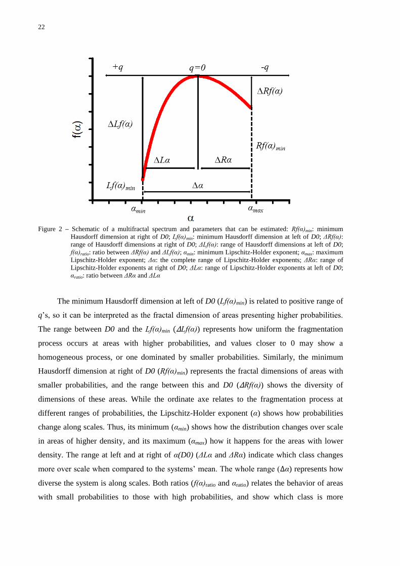
Figure 2 – Schematic of a multifractal spectrum and parameters that can be estimated: Rf(α)min: minimum

Hausdorff dimension at right of D0; Lf(α)min: minimum Hausdorff dimension at left of D0; ΔRf(α):

range of Hausdorff dimensions at right of D0; ΔLf(α): range of Hausdorff dimensions at left of D0;

f(α)ratio: ratio between ΔRf(α) and ΔLf(α); αmin: minimum Lipschitz-Holder exponent; αmax: maximum

Lipschitz-Holder exponent; Δα: the complete range of Lipschitz-Holder exponents; ΔRα: range of

Lipschitz-Holder exponents at right of D0; ΔLα: range of Lipschitz-Holder exponents at left of D0;

αratio: ratio between ΔRα and ΔLα

The minimum Hausdorff dimension at left of D0 (Lf(α)min) is related to positive range of

q’s, so it can be interpreted as the fractal dimension of areas presenting higher probabilities.

The range between D0 and the Lf(α)min (ΔLf(α)) represents how uniform the fragmentation

process occurs at areas with higher probabilities, and values closer to 0 may show a

homogeneous process, or one dominated by smaller probabilities. Similarly, the minimum

Hausdorff dimension at right of D0 (Rf(α)min) represents the fractal dimensions of areas with

smaller probabilities, and the range between this and D0 (ΔRf(α)) shows the diversity of

dimensions of these areas. While the ordinate axe relates to the fragmentation process at

different ranges of probabilities, the Lipschitz-Holder exponent (α) shows how probabilities

change along scales. Thus, its minimum (αmin) shows how the distribution changes over scale

in areas of higher density, and its maximum (αmax) how it happens for the areas with lower

density. The range at left and at right of α(D0) (ΔLα and ΔRα) indicate which class changes

more over scale when compared to the systems’ mean. The whole range (Δα) represents how

diverse the system is along scales. Both ratios (f(α)ratio and αratio) relates the behavior of areas

with small probabilities to those with high probabilities, and show which class is more

23

fragmented and changes more across scale, respectively. They are calculated according to

Equations 26 and 27.

(26)

(27)

2.1.1.4 Fractal and multifractal applications in soil science

Fractal techniques have been used in soil science as an alternative to conventional

geometry (PACHEPSKY et al., 1996; GIMENEZ et al., 1997). The fractal dimension

assumes that a soil property is scale dependent and can be represented by a power law. In soil

biology it was used in evaluation of mycelial morphology of different fungi species (BODDY

et al, 1999). In the soil chemistry area, Rice and Lin (1993) were the first to evaluate the

fractal nature of humic materials, followed by Senesi (1999), Rizzi et al. (2004) and Fedotov

and Shoba (2013). Also Rice et al. (1999) and Sokolowska et al. (2009) considered patterns of

the distribution of soil organic matter. Fractal dimensions were also used in many other areas

of soil chemistry, e.g., as a parameter to estimate cation exchange capacity (ERSAHIN et al.,

2006; BAYAT et al., 2014), to evaluate mineral dissolution (GUARRACINO et al., 2013),

nitrogen adsorption isotherms (PAZ FERREIRO; WILSON; VIDAL VÁZQUEZ, 2009), soil

metal contamination (GERANIAN; MOKHTARI; COHEN, 2013), amongst others.

The field of soil physics is where the use of fractal analysis started, and, because of that,

is the area with most vast use for such theory. It started in the analysis of soil particles

distribution (ORFORD; WHALLEY, 1983), and have been widely used until today for the

same purpose (TYLER; WHEATCRAFT, 1992; STANCHI et al, 2006, BIEGANOWSKI et

al., 2013; PENG et al., 2014). In the analysis of the structure Turcotte’s (1986) paper on soil

fragmentation was a pioneer, while publications by Young and Crawford (1991), and

Crawford, Sleeman and Young (1993), are the classical base for fractal modeling of

aggregates size distribution. In the field of pore analysis its use was really expanded,

especially considering the image analysis of soil pore systems. The first work considering the

pore system was the one from Rieu; Sposito (1991), and was followed for more than 30

publications on the same subject, considering methodological problems and specific

applications. There are several review papers about fractal under the structure scope.

Ghanbarian-Alavijeh et al. (2011) reviewed the pore-solid-fractal approach; Perfect and Kay

24

(1995) the applications in soil and tillage researchs. All things considered, the fractal theory

was, and still have been, well explored in soil science.

However, the fractal approach characterizes the mean properties of a dataset and cannot

provide information on average behavior deviations of a power law (POSADAS et al., 2003).

The multifractal analysis includes density variations and can be expressed in a multifractal

spectrum (CHHABRA et al., 1989; CHHABRA; JENSEN, 1989), which integrates and

quantifies the spatial properties of the studied object (POSADAS et al., 2003). The

multifractal tool is much newer if compared to the fractal approach, especially applied to the

soil science field. For example, during the literature review for this research, it was found 10

papers which used multifractal analysis for particle size distribution, 4 in the analysis of soil

structure and 21 considering the pore system, being 5 about water retention modeling. The

respective number of papers considering the fractal applications were 19, 46, 27 and 45.

Some parameters of the multifractal spectrum are well known and related to the

heterogeneity of the porous system (POSADAS et al., 2003). However, due to its still

incipient use in soil science, soil properties leading to a multifractal behavior are not

established yet, which makes the interpretation of soil multifractal parameters an important

subject of investigation.

2.1.2 Definition of soil physical quality – stability and functioning

The description of any system demands the creation of an ordered list of parameters

with specific definitions that allows us to explain each step of the phenomena occurring in

such system. Let us take as example the term “soil science”. Before knowing its significance,

it is necessary to define separately what is “soil” and what is “science”. Soil (from Latin

solum, Anglo-French soy and Middle-English soile, meaning “ground”) can be defined as a

triphasic (consisting of air, liquids and solids) and tridimensional body that occupies the

Earth’s surface. It is bordered by the atmosphere above, the lithosphere below and by water

bodies laterally (i.e. lakes, rivers, seas and oceans) and beholds life. Its genesis arises from the

interaction between a parental material with climate and organisms over time, being affected

by the relief. Science (from Latin scientia, meaning "knowledge") is a systematic enterprise

that builds and organizes knowledge in the form of testable explanations and predictions

about the universe. Science is also associated with the scientific method itself, which the

Oxford English Dictionary (2015) defines as "a method or procedure … consisting in

systematic observation, measurement, and experiment, and the formulation, testing, and

modification of hypotheses". Thus, “soil science” can now be defined as a systematic

25

organization of the knowledge achieved of the subject “soil” by experimentation. It is

developed by the study of soil as a natural resource of the surface of the Earth, based on the

description of its genesis, classification and mapping, using physical, chemical and biological

attributes, and aiming to enhance its use, management and conservation.

Although very broad, we can follow the same premise to define “soil physical

quality”. Is important to state that the aim of this work is not to create a global definition for

this term, but the reader needs to understand our scope when referring to it during this text. A

brief comment on the definition of soil structure is needed. As stated before, soil is triphasic.

How the three phases interact forming different arrangements between solids and pores (i.e.

the spaces not occupied by solids that can be filled up by liquid or air) is defined as “soil

structure”.

“Soil quality” can be defined as “the ability of a soil to perform functions that are

essential to people and the environment” (DORAN et al., 1994). Since soil structure affects

water and air movement, influencing its ability to execute vital functions, and all of the above

are physical processes occurring in soil, the term “soil physical quality” will be considered in

this text as a measure of the ability that soil structure has to perform functions that are

essential to mankind and the environment. Thus, a soil with good physical quality presents a

soil matrix resistant to disaggregation, at the same time allowing life to exist. In other words,

a soil with high physical quality must be resistant to erosion and exhibit a degree of

organization that allows the development of flora and fauna.

All classical soil physical properties (texture, bulk density, aggregates shape and size)

allow inferences about soil physical quality, because they all relate to the matrix arrangement.

However, it is common to find that most publications on soil physical quality are associated to

some physical index, in an attempt to resume several soil attributes into fewer variables. Such

index may be linked to properties that command crop development, like compaction and

resistance to penetration. Some examples are the aggregates tensile resistance (DEXTER;

KROESBERGEN, 1985; MULLINS et al., 1992), relative bulk density (HÅKANSSON,

1990) and the least limiting water range (SEVERIANO et al., 2011). On the other hand, soil

structural stability, which is a measure of how soil structure maintains its coherence over

time, is also an important physical qualifier. In this case, clay dispersion (LEVY et al., 1993)

and distinct measures of aggregates stability (Le BISSONNAIS, 1996) are widely used to

produce indexes, since they show how soil behaves against erosion.

We can consider the soil functioning as the third pillar of soil physical quality. The term

“function” relates to how the soil plays its role in the ecosystem. Then, its “functioning” is

26

any process that leads to this end. The main physical processes in soil are modeled via flux

equations. These are used to model water (RAATS, 2001) and air (MOLDRUP et al., 2001)

movement in soil. In that way, properties that represent these processes are also indicative of

the degree of physical quality of a soil. Examples are the use of the classical water retention

curve (DEXTER, 2004a, 2004b), the surface water infiltration rate (ZHOU; LIN; WHITE,

2008), the air permeability (BALL et al., 1997), hydraulic conductivity (PAGLIAI;

VIGNOZZI; PELLEGRINI, 2004), amongst others. Some of these will be explored in this

text.

2.1.3 Soil erosion: its mechanic and the “sealing” process

Soil erosion is a set of natural processes that changes a soil, diminishing its capability

on exercising its function in the ecosystem. These processes cause physical, chemical and

biological changes. They are marked by: the selective removal of particles, which changes the

structure, interfering in the dynamics of fluids and heat; the decline in the content of organic

matter and nutrients, causing decay in soil fertility; and, as a result, a reduction in the biota.

Human accelerated erosion is a major cause of cultivable soils depletion, making them

unsuitable for exploitation. To change this feature, several soil conservation techniques are

used to reduce erosion to a minimum rate. These techniques are the result of extensive

research on the causes of erosion, which are explained by the mechanics of the erosion

process, that relates the soil and the erosive agents.

2.1.3.1 Physical Erosion

It is common to divide erosion into physical, chemical and biological, according to its

cause (LAL, 2001). The physical erosion is the process in which a natural agent causes the

breakdown, transport and deposition of soil particles and aggregates (MORGAN, 2005).

During this text we will only discuss this type of erosion and address it simply by “soil

erosion”.

The natural agents cited above are any force of nature capable of implementing

sufficient energy to detach soil particles and aggregates, and move them, until they deposit at

a location different from its origin. Wind and water are those agents, but they may be assisted

by fire (SHAKESBY, 2011; GABET, 2014), since fire weakness the structure, and gravity as

supporter agents (LAL, 2001). However, wind or water are still needed to detach and carry

the soil to a lower gravitational reference (e.g. point closer to earth’s center).

27

In the case of water, erosion may occur due to its performance in liquid form, through

the action of rainfall, rivers and sea waves (LAL, 2001), or in solid form, due to expansive

action of water during the condensation process, or to the melting that destabilizes the

structure (ANDERSLAND; WIGGERT; DAVIES, 1996). In tropical regions, which

represents a major area of Brazil, the main erosion agent is rainwater, since summer

rainstorms are very common in such climate. The rainfall is primarily responsible for the

erosion in places where the soil bares unprotected, due to tillage operations, and prone to

crumbling.

2.1.3.1.1 Mechanics of erosion caused by rainfall

2.1.3.1.1.1 Rainfall erosivity and soil erodibility

Considering rainfall itself, several attributes interfere in its “erosivity”, i.e. its capacity

in causing erosion (WISCHMEIER; SMITH, 1960; SALLES; POESEN; GOVERS, 2000).

We can summarize the main attributes as: the raindrop size (UIJLENHOET; STRICKER,

1999), pressure exerted over the soil (NEARING; PARKER, 1994) and velocity when

reaching the target (GUO et al., 2013); the rainfall intensity (ASSOULINE; BEN-HUR, 2006)

and amount (DALLA ROSA et al., 2012); and the composition of the rainwater (BORSELLI

et al., 2001). Most studies on soil erosion process keep one or two of these attributes as

variables, while maintaining all others constant. In studies with simulated rainfall, the

raindrop size, velocity, pressure and angle of contact can be controlled by the devices sets.

Then, is left to the researcher to decide on the intensity and amount to be used during

experimentation.

Once rainfall impacts on soil surface, the erosion starts to be controlled by its intrinsic

properties, such as: soil type and steepness, that are dependent on the parental material,

regional climate and landform (WISCHMEIER; MANNERING, 1969); tillage and cover,

factors that are controlled by man (i.e. land use) (DALLA ROSA et al., 2012). Once again,

these are attributes that can be controlled or evaluated separately, to comprehend their

relationship with erosion rates (VAN OOST; GOVERS; DESMET, 2000; LAL, 2001).

Rainfall erosion begins with the impact of raindrops over the soil surface (NEARING;

BRADFORD; HOLTZ, 1987), continues through disintegration of clods and aggregates (Les

BISSONNAIS, 1996), extends up to the runoff (NEARING; PARKER, 1994) and it ends with

the sedimentation. Part of the sediments formed during the rainfall event are carried along

with the water to the watercourses and are deposited in the lower parts of the relief (e.g.

riparian zones). However, part of these particles and aggregates can also settle very close to

28

its origin, causing local changes in soil surface structure by forming a “seal”. Since the whole

erosion process consists of these three main steps (particles and aggregates detachment, runoff

and sedimentation) this will be further discussed.

2.1.3.1.1.2 Particles and aggregates detachment and transport

The detachment of the particles is the first stage of the erosion process and occurs

mainly by three causes: the raindrop impact, which releases its kinetic energy on the soil

surface, breaking aggregates and clods where the structure has weak points, and spreading

particles around; slaking, due to rapid moistening, that increases aggregates internal pressure,

causing micro-implosions that create ruptures that induce crumbing; and by water induced

structure weakness, since water acts as a lubricant that allow structural sliding when soil is

saturated (Les BISSONNAIS, 1996).

The second stage of erosion is the transport of aggregates and particles. It starts with the

spreading caused by the impact of the raindrop, and continues when water starts to flow in

surface, carrying sediments downhill (MORGAN, 2005). Water surface flow only happens if

rainfall intensity exceeds soil hydraulic conductivity capacity (DARBOUX et al., 2001). To

be transported, the sediment must be detached from the soil matrix (SHARMA, 1996), and

the rate and distance is dependent on the energy of the water flux at surface (DARBOUX at

al., 2001), which is dependent on the steepness (NEARING; PARKER, 1994) and roughness

of the surface (DARBOUX; HUANG, 2005). During the superficial flux of particles, i.e. the

runoff, more particles can be detached and transported, depending on the shear capacity of the

flux and the shear resistance of the soil (HUANG; BRADFORD; LAFLEN, 1996).

If the water flow at surface is laminar, particles removal is of uniform thickness over the

area, causing what is called as sheet or interrow erosion (DESCROIX et al., 2008). When the

flux concentrates and the flow becomes turbulent, soil removal occurs by forming intermittent

rills (MORGAN, 2005). If these evolve to become persistent and deeper, the so called gullies

are formed. In the current specialized literature, these have been divided into ephemeral

gullies and gullies according to their depth and width (CHESWORTH, 2008).

2.1.3.1.1.3 Particles and aggregates deposition – sealing and crust formation

The last step of the erosive process is the deposition of particles and aggregates that

were detached from the soil matrix. The deposition happens according to the size and weight

of sediments. The first particles and aggregates to deposit are those with low transportability,

i.e. the heavier and wider ones (BERTONI; LOMBARDI NETO, 2005). The lightest

29

materials are the last ones to deposit, reaching larger distances from its origin. The runoff

flow energy also influences the morphology and distribution of particles. Irregular depositions

suggest erosive events with turbulent flow, while uniform deposits, with well-selected grain

sizes, are an indicative of laminar flow (MOMOLI et al., 2007).

Sediments properties differ according to their origin and, many times, can be

distinguished from local horizons by color, particles size distribution, organic carbon content,

pH and exchange complex constitution (FULLEN et al., 1996). Local sediments are, in

essence, of coarser fractions, since clay and silt can be transported through larger distances.

The amount of clay and silt also increases in proportion to the slope, since the steeper slopes

contribute to the acceleration of runoff, increasing the soil erodibility. Hence, parental

material, relief and precipitation are the determinant factor influencing the size distribution of

the sediments.

The deposition of particles and aggregates over the original soil surface forms a layer

with different structure from the one underlying. The increase in thickness of this layer may

change the surface bulk density, due to an decrease in the porosity, followed by an decrease in

its hydraulic properties, fact why this layer is called a “soil seal”. When this layer of soil dries

out, is common to occur an increase in the resistance to penetration, while its aspect becomes

brittle and laminar, forming a so called “soil crust”. Although sometimes the terms soil

crusting and soil sealing are considered as synonymous, soil sealing describes the wet process

in which porosity decreases due to a rearrangement of structure, while soil crusting marks the

increase in soil strength due to the drying of this rearranged structure (BERGSMA et al.,

2000).

Considering the above, crusts can be separated into two types: structural and

depositional. These two types give birth to different microstructure morphologies, and may

occur successively, initiating with the sealing of the surface by an structural brokenness,

followed by an depositional process of particles on its top. Structural crusts are formed by the

reorganization of the soil surface due to a local displacement of fragments, i.e., clods and

aggregates, without the sedimentation of particles. They are the result of gradual packaging

and coalescence of small clods and aggregates, which are mainly produced by the breakdown

of bigger aggregates due to an increased internal stress during wetting, i.e., slaking

(NORTON; SCHROEDER; MOLDENHAUER, 1986). Depositional crusts are the result

from the displacement of fragments and particles due selective decantation in puddles, formed

during the runoff process, where the water slowly infiltrate into the soil (KOOISTRA;

SIDERIUS, 1986).

30

2.1.4 Soil surface roughness vs soil physical quality

The behavior of the soil surface structure has an important role on air, water and

nutrients dynamics. In tropical and subtropical regions it is common to have high intensity

rainfall events during summer seasons, and rainfall erosivity can lead to greater problems on

bare and/or tilled soil. The raindrop impact changes soil microtopography, which controls

surface depressional water storage (BURWELL et al., 1963; HANSEN et al., 1999;

BORSELLI; TORRI, 2010), drainage and runoff (SEGINER, 1969; ROMKENS et al., 2001),

and even interferes on infiltration rates (BURWELL; LARSON, 1969; MAGUNDA et al.,

1997; GUZHA, 2004). Therefore, the state of the soil microtopography is dependent on, and

controls, soil erosion (MAGUNDA et al., 1997; DARBOUX et al., 2005; RODRÍGUEZ-

CABALLERO et al., 2012).

Very often, the roughness of a surface is a measure of its state. Smith (2014) ratify that

“surface roughness” generically defines any “…resulting parameter…that determines the

minimum amount of information necessary to parameterize topographic complexity at a

degraded scale in the most physically meaningful way”. He also states that this is subjective

and dependent on the objectives of a study. Therefore, in soil science, the surface roughness is

considered as a parameter that represents the variability of a set of (z) heights inside an (x, y)

area and can be used to interpret the morphology of the microtopography. Commonly, this

parameterization separates roughness into two classes: the Oriented Roughness, governed by

the slope and tillage marks, and the Random Roughness (RR), representing the distribution of

soil clods and particles (ALLMARAS et al., 1966; CURRENCE; LOVELY, 1970;

KAMPHORST et al., 2000). The latter one, a major percentage of total roughness, is the most

relevant considering fluxes at surface, since it controls the dynamics of runoff and it is

governed by soil intrinsic attributes (i.e. particles and clods size distribution, water dispersed

clay and aggregates stability).

Consequently, several devices that collect data are used to estimate roughness

parameters. The pin meter (BURWELL et al., 1963), the laser profilometer (CURRENCE;

LOVELY, 1970) and the infrared microrelief meter (MRM) (CASTRO et al., 2006;

CASTILHO et al., 2011) are examples of equipments used in field, that perform readings of

(z) heights in square grids with a (x,y) resolution ≥ 1 mm. Other devices, generally used in the

laboratory, case of Huang’s laser scanner (HUANG et al., 1988) and the Multistripe Laser

Triangulation (MLT) scanner (HIRMAS et al., 2016), reach finer horizontal resolutions, up to

0.5 mm. In addition, computed tomography allows the generation of even higher resolution

images, as far as 0.02 mm (20 µm) by using standard X-ray computed tomography (XRT)

31

(ELLIOT; REYNOLDS; HECK, 2010) or even 0.001 mm (1 µm) using X-ray

microtomography (µXRT) (ZHOU et al., 2013). Information on increasing scales stimulates

the study of fragmentation processes caused by rainfall, because it allows mapping clods

disruption by reaching scales close to the actual size of the soil’s primary particles, which was

only possible previously via mathematical and/or statistical modeling. Furthermore, the

gathering of real physical data on different scales can help enhance models used to estimate

more complex variables (i.e. drainage, runoff, soil loss).

Apart from the above, the roughness parameterization depends on distinct mathematical

approaches as well. Allmaras et al. (1966) first used the standard error of log of heights, and

Currence and Lovely (1970) showed the standard deviation of heights was enough if Oriented

Roughness was corrected. Since these indexes only represent the vertical range of roughness,

without considering the spatial component (KAMPHORST et al., 2000), several authors tried

a geostatistical approach (VIDAL VÁSQUEZ et al., 2009; DALLA ROSA et al., 2012).

However, the scale factor is also important and fractal models were also used in conjunction

to spatial modeling (HUANG; BRADFORD, 1992; VIDAL VÁSQUEZ et al., 2005, 2010).

Two facts restrain the use of fractal theory on roughness analysis: (1) it relies on a single

number to describe the whole system; (2) although fractal indices may represent

morphological responses to rainfall, they cannot be used to actually quantify fluids dynamics

at the surface (KAMPHORST et al., 2000). In this sense, multifractal models excel. The

multifractal approach consider several dimensions related to local occurrence of probabilities

of a process, which merges the information of scale and spatial distribution, making it

possible to generate indexes that may be used to model complex variables. This rising

technique in soil science is still little explored in the evaluation of surface roughness

(GARCÍA MORENO et al., 2008; SAN JOSÉ MARTÍNEZ et al., 2009; VIDAL VÁSQUEZ

et al., 2010), but it is very promising in the generation of parameters that may express

structural changes of the soil surface.

2.1.5 Soil structure image analysis

Micromorphometrical analysis consists on the evaluation of thin sections taken from

soil blocks impregnated with polyester resin. This technique allows the study of the soil

microstructure and to quantify the shape, size and soil pore connectivity using quantitative

indexes related to pores and aggregate morphology (RINGROSE-VOASE, 1987; HORGAN,

1998; HOLDEN, 2001). Since the pore system morphology is related to water movement and

the matrix arrangement is associated to pedogenic processes and biological activity (BOUMA

32

et al., 1977; RINGROSE-VOASE, 1987; PAGLIAI; DENOBILI, 1993) this technique has

aided in the study of the soil structure (RINGROSE-VOASE; BULLOCK, 1984).

The selection and interpretation of soil pore morphological parameters still requires

research (DROOGERS et al., 1998; HOLDEN, 2001) and, although this approach allows to

systematically analyze a soil sample, it provides a partial result, since the analysis are made in

two-dimensional soil sections.

The computed tomography scan is an alternative to the bidimensional problem. This is a

relatively new technique in soil analysis, since X-rays were discovered only in the late

nineteenth century by WC Roentgen (HECK, 2009). The X-rays attenuation index calculus

obtained mathematical foundations only in 1963 by Cormack (CARVALHO, 2007) and initial

works using this technique to study the soil emerged only in the 1980s. It was widely used in

the study of soil porosity and hydraulic properties, initiating with innovative studies in the

1980s, related to soil bulk density (HAINSWORTH; AYLMORE, 1983), water movement in

soil-plant system (PETROVIC et al., 1982) and soil moisture (CRESTANA, 1985). In the

early 1990s, it was used aiming to understand the structure morphology and behavior, by

macroporosity measurements (PHOGAT; AYLMORE, 1989; GREVERS et al., 1989;

ANDERSON et al., 1990), biopores reconstruction (JOSCHKO et al., 1992, 1993) and effect

of aggregate size on solute transportation (ANDERSON et al., 1992). In the late 1990s and

early 2000s, the main use of this technique switched to understanding structure modifications

in soils, such as due to cropping system (OLSEN; BØRRESEN, 1997), decomposition of

organic waste (De GRYZE et al., 2006) and to wetting and drying cycles (PIRES et al., 2007).

Nevertheless, although the studies using CT brought a new approach to image analysis,

there was not a distinguished language used to describe soil structural quality that implicated

in a leap between these and classical techniques. And the calculation of indexes that are

actually based on a tridimensional approach is still scarce, since much work has been done

analyzing the bidimensional slices that form the reconstructed 3d image.

2.2 Material and methods

An experiment with simulated rainfall was assembled on a Fine Rhodic Kandiudalf

(SOIL SURVEY STAFF, 2014), i.e., a Nitossolo Vermelho eutroférrico argiloso

(EMBRAPA, 2013), located at 22º41’51.5” S and 47º37’53.2” W, at the “Luiz de Queiroz”

College of Agriculture – University of Sao Paulo, in the city of Piracicaba, Sao Paulo, Brazil

(Figure 3). Piracicaba is in an altitude of 554 meters, in a subtropical region of the state of Sao

Paulo. Its climate is Cwa, according to the classification of Köppen-Geiger. Temperatures

33

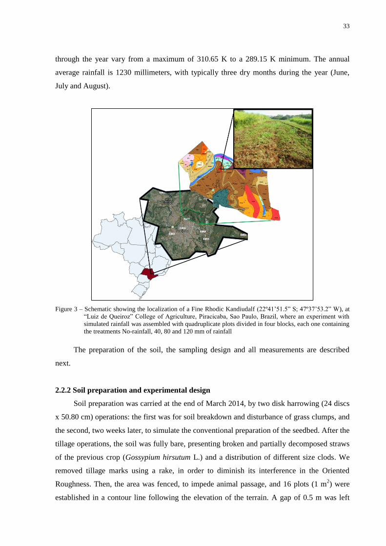
through the year vary from a maximum of 310.65 K to a 289.15 K minimum. The annual

average rainfall is 1230 millimeters, with typically three dry months during the year (June,

July and August).

Figure 3 – Schematic showing the localization of a Fine Rhodic Kandiudalf (22º41’51.5” S; 47º37’53.2” W), at

“Luiz de Queiroz” College of Agriculture, Piracicaba, Sao Paulo, Brazil, where an experiment with

simulated rainfall was assembled with quadruplicate plots divided in four blocks, each one containing

the treatments No-rainfall, 40, 80 and 120 mm of rainfall

The preparation of the soil, the sampling design and all measurements are described

next.

2.2.2 Soil preparation and experimental design

Soil preparation was carried at the end of March 2014, by two disk harrowing (24 discs

x 50.80 cm) operations: the first was for soil breakdown and disturbance of grass clumps, and

the second, two weeks later, to simulate the conventional preparation of the seedbed. After the

tillage operations, the soil was fully bare, presenting broken and partially decomposed straws

of the previous crop (Gossypium hirsutum L.) and a distribution of different size clods. We

removed tillage marks using a rake, in order to diminish its interference in the Oriented

Roughness. Then, the area was fenced, to impede animal passage, and 16 plots (1 m2) were

established in a contour line following the elevation of the terrain. A gap of 0.5 m was left

34

between plots to avoid drifts from neighboring treatments. A random blocks design divided

the contour line in 4 blocks wherein rainfall applications were randomized (Figure 4).

Figure 4 – (a) Picture of a Rhodic Kandiudalf after the second passage of a leveling harrow, (b) image showing

how was the slope of the area and the localization of the water tank, and (c) leveled photo from the 1

m2 plots, demarcated by a black/yellow tape and arranged in a line perpendicular to the slope. (d) The

scheme of the experimental design in randomized blocks (d), showing how the blocks were divided

along the line and an example of how the rainfall was randomized within each one of the four blocks.

After rainfall application (item 2.2.3), following a 24 h drying period, elevation data

was collected from each plot with a laser microrelief meter (item 2.2.4). Six undisturbed

samples were collected by plot: two soil blocks (12 x 12 x 5 cm) were scanned by a

multistripe laser triangulation (MLT) scanner and a X-ray tomography (XRT) scanner,

respectively, to obtain information about surface roughness (item 2.2.4); two cylinders (2.5 x

5 cm) were collected to measure the bulk density (item 2.2.5.2), and to model the water

retention curve (item 2.2.5.3); two soil blocks (12 x 7 x 5 cm) were used in aggregate stability

tests (item 2.2.5.2) and micromorphometrical analyses (item 2.2.6.1). One disturbed sample

was collected by experimental block at the surface (0-5 cm), to characterize the soil particles

distribution (item 2.2.5.2), pH and exchange complex composition (item 2.2.5.1) (Figure 5).

35

The particles size distribution and chemical composition of the exchange complex are

summarized on Table 1 and Table 2. The blocks were homogeneous. However, during

statistical procedures the block design was maintained due to other possible causes of

variance (e.g. terrain slope, machinery passage, etc.).

Figure 5 – (a) Disposition of the sampling inside each plot and (b) scheme with the measures of each sample:

two cylinders with 50 mm in diameter, that were used for bulk density and water retention curve

evaluations; two rectangular blocks (120 x 70 mm), that were used in micromorphometrical and

aggregates stability analyses; and two square soil blocks (120 mm x 120 mm) that were used in

roughness analyses. The dots represent the resolution of roughness measurements. A field

microrelief meter was used to gather information of the whole 1 m2 plot (10 mm resolution). For

each square soil block there were different scales of measurement, using a multistripe laser scanner

(right, 0.5 mm resolution) and a X-ray tomography scanner (left, 0.074 mm resolution). Solid lines

represent the area of collected data, while dashed lines represent the cropped area used during

analyses. The arrow in the middle indicate the position of the infiltrometer, used to measure

unsaturated soil hydraulic conductivity

36

Table 1 – Values of pH, organic carbon content (OC) and particles size distribution of a Fine

Rhodic Kandiudalf (22º41’51.5” S, 47º37’53.2” W) at surface (0-5 cm) after two

disk harrowing operations

Block pH Clay Silt Sand OC

H2O CaCl2 KCl

g kg-1

1

6.1 5.4 5.0

521 222 257 15.99

2

6.2 5.5 5.1

547 205 248 15.23

3

6.2 5.5 5.1

547 211 241 15.23

4 6.1 5.5 5.1 547 210 243 14.85

Table 2 – Chemical composition of the exchange complex of a Fine Rhodic Kandiudalf

(22º41’51.5” S, 47º37’53.2” W) at surface (0-5 cm) after two disk harrowing

operations

Block P K Ca Mg Al H+Al SB CEC V M

mg Kg-1

mmolc kg-1

%

1 0.198

10.61 52.91 23.00 0.00 0.60 86.52 87.12

99.31 0.00

2 0.148

10.87 54.56 22.54 0.00 11.60 87.97 99.57

88.35 0.00

3 0.119

9.08 55.11 23.36 0.00 9.00 87.55 96.55

90.68 0.00

4 0.122 12.02 52.58 23.81 0.20 18.00 88.42 106.42 83.09 0.23

P:phosphorus; K: potassium; Ca: calcium; Mg: magnesium; Al: exchangeable aluminum; H+Al: hydrogen and

aluminum (soil potential acidity); SB: sum of bases; V: base saturation; m: aluminum saturation

2.2.3 Rainfall simulation

Rainfall was applied at an intensity of 120 mm h-1

in the quadruplicate plots at amounts

of 40, 80, and 120 mm, plus a control treatment with no-rainfall. The simulator operates at a

height of 2.4 m above the soil and consists of a oscillating spray nozzle (VeeJet Nozzle, H/U-

80100, Spraying Systems, Co.) connected to a system that maintain a pendulum movement to

simulate rainfall in a total area of 1m2. The entire system is supported by metal pipes that

brings lightness and firmness at the same time. To avoid the effects of drift a plastic cover

was placed around the equipment (Figure 6a).

The rainfall intensity was chosen based on regional climate characteristics and soil

structural features. For example, Hudson (1965) stated that rainfall intensities over 25 mm h-1

are erosive for most tropical and subtropical soils. However, soil erosion is a combination

between rainfall erosivity and soil erodibility, which depends on intrinsic properties of soil,

such as structural stability. Castilho et al. (2011), studying the same soil of this research

(Rhodic Kandiudalf), found undisrupted clods even after 10 natural rainfalls with intensities

higher than 25 mm h-1

. Magunda et al. (1997), in a similar soil (Mollic Kandiudalf), found

minimal changes on soil surface roughness after 126 mm of simulated rainfall with an

intensity of 63 mm h-1

. These are evidences that such soils possess a highly stable structure.

37

Considering that, to fully understand this soil disruption behavior due to cumulative

rainfall, higher intensities must be used during simulation tests, so that a wider range of

structural changes may be captured.

2.2.4 Soil surface roughness measurements

The evolution of the surface roughness was evaluated in three scales of measurement. In

the field, a portable field microrelief meter (MRM) was used, coupled with an infrared sensor

(GP2Y0A21YK0F, SHARP Corporation) with ±0.05 mm resolution, and making readings on

a fixed grid (10 x 10 mm), totaling 10,201 points per plot (Figure 6a). In the laboratory two

finer scales were obtained from soil blocks. One block from each plot was scanned by a

multistripe laser triangulation (MLT) scanner (NextEngine, Inc.), creating a random mesh

averaging 60,000 points (resolution of 0.5 mm) (Figure 6c). A second block from each plot

was scanned using an X-ray tomography (XRT) scanner model XT H 225st, third generation,

with a total of 1918x1534 detectors (Figure 6b). To reduce artifacts and image noise a high

passage filter was used. The acquisition voxel size was of 74.5 x 74.5 x 74.5 µm. This process

results in average of 3018 two-dimensional projection images that are reconstructed to portray

a three-dimensional soil structure. The final image was reconstructed using maximum

resolution, and the process was filtered by back projection, using CT PR O 3D and

VGSTUDIO.

To minimize influences of artifacts and disturbances on samples edge, only a central

area from each resulting mesh was analyzed, cropping areas of 800 x 800 mm, 75 x 75 mm

and 30 x 30 mm for MRM, MLT and XRT, respectively.

2.2.5 Soil attributes

2.2.5.1 Chemical analyses

The determinations of pH in water, CaCl2 0.01 mol L-1

, KCl 1 mol L-1

, and of the

content of exchangeable aluminum (Al), potassium (K), phosphorus (P), calcium (Ca) and

magnesium (Mg) were performed according to Raij et al. (2001). The Walkey-Black method

was used for the determination of the organic carbon content (OC), as described in Anderson

and Ingram (1992). All soil samples were air dried and sieved (< 2 mm) prior to each

analysis.

38

Figure 6 – (a) Rainfall simulator (with a blue cape) and field microrelief meter (MRM) sensor (black device); (b)

X-ray tomography (XRT) third generation scanner, with a total of 1918x1534 detectors (c) multistripe

laser triangulation (MLT) scanner; (d) soil block (120 x 120 mm) aligned at 150º and ready to be

scanned by the MLT scanner; (e) example of a reconstructed image using the MLT accompanying

software

2.2.5.2 Physical analyses

The bulk density (BD) (Mg m-3

) was determined using the cylinder method according to

Grossman and Reinsch (2002). Cylinders (2.5 x 2.5 cm) were collected in quadruplicates by

rainfall amount. The particle size distribution was determined by the hydrometer method

(GEE; OR, 2002), using 40 g of sieved disturbed samples (< 2 mm) after air dried. The

number of replicates was the same as for the cylinder method used for BD. The particles

density (PD) (Mg m-3

) was determined from the same disturbed samples (< 2 mm) using a

Helium pycnometer (AccuPyc 1330, Micromeritics Instrument Corporation ®). The ratio of

volume of pores (Pr) (m 3 m

-3) was calculated from BD and PD (Equation 28), indicating the

relative amount of voids of the soil (VOMOCIL, 1965).

(28)

An aggregates stability test was conducted according to Le Bissonnais (1996) using

blocks of soil (12 x 7 x 5 cm) collected in quadruplicates according to rainfall amount. The

surface of each block (0-10 mm) was ripped off, from which, aggregates were manually

39

broken and normalized to a diameter between 4 and 2 mm. The 10 mm layer was chosen in an

attempt to boost the chances of detecting the changes caused by sealing. After, pre-treatments

were applied in triplicates of 5 g of normalized aggregates, dried at 313,15 K for 24 h. The

pre-treatments were: slow wetting, where dry aggregates were placed in a filter paper over a

saturated sponge and slowly moistened by capillary forces; fast wetting, where dry aggregates

were submerged directly into water; and mechanical breakdown, when dry aggregates were

previously moistened with alcohol and shaken, while submerged in water, with controlled

energy. After each pre-treatment, the aggregates were immersed in alcohol and sieved (0.053

mm), with the retained soil once again dried (313,15 K for 24 h). These dry aggregates were

then passed through a set of six sieves (2, 1, 0.5, 0.106 and 0.053 mm), generating an

aggregates size distribution, which was consequently used to calculate the weighted mean

diameter (WMD) (Equation 29).

(29)

WMD considers the equivalent diameter of aggregates ( ), which is the average

diameter between a subsequent set of sieves (e.g. between sieves 2 mm and 1 mm = 1.5

mm), having the relative mass of aggregates (

) as weights. is the total mass of

aggregates (5 g) and is the mass of aggregates retained at each sieve i.

2.2.5.3 Hydrological analyses

Soil water retention curve (SWRC): The SWRC is the correlation between the

gravimetric water content (θ) and the matric potential in the soil (Φm). Undisturbed soil

samples were collected in cylinders (2.5 x 2.5 cm). Using a nylon string, each cylinder was

subdivided into three parts (top, middle and bottom) while maintaining the original structure.

The subsamples were relocated to smaller cylinders (2.5 x 0.8 cm). Since there were

quadruplicate samples for each rainfall amount, it totaled 48 subsamples. Curves were

generated using these subsamples in pressure plates for potentials of -0.001; -0.003; -0.006; -

0.008; -0.010; -0.033 -0.070 MPa and -0.100, and disturbed samples (< 2 mm) in high

pressure plates for potentials of -0.300, -0.500 and 1.5 MPa. The curves were fitted using the

empirical model proposed by van Genuchten (1980), which parameters are the soil water

contents at saturation θs and residual θr, plus the empirical parameters n and α (Equation 30).

Changes in the inclination of the curves were evaluated using parameters n and α.

40

(30)

Soil hydraulic conductivity [K(θ)]: The hydraulic conductivity of the unsaturated soil

was calculated by measurements with a mini disk infiltrometer (Mini Disk Infiltrometer,

Decagon Devices) at four potentials (-1.5, -3.0, -4.5 and -6 cm) (Figure 5). To calculate the

unsaturated hydraulic conductivity, the method by Zhang (1997) was used.

2.2.6 Image analyses

2.2.6.1 Micromorphometrical analyses

Undisturbed soil samples, oriented to the surface and collected in cardboard boxes (0.12

x 0.07 x 0.05 m), were impregnated using a polyester resin (MURPHY, 1986), styrene

monomer (CASTRO et al., 2003), a catalyzer (RINGROSE-VOASE, 1991) and a fluorescent

pigment (MURPHY et al., 1977). The impregnation procedure and image acquisition was

done as described by Castro et al. (2003).

In the laboratory, the samples were air dried for 10 days and at 313.15 K with forced air

circulation for 48 hours. These samples were put in containers and placed in a desiccator

connected to a vacuum pump, which helps the solution to penetrate the pores. The

impregnation was held by a solution of polyester resin and styrene monomer (1/1), using a

hardening solute (Butanox M50, 10 drops L-1

of solution) and a fluorescent colorant (Tinopal

OB, Ciba-Geigy®, 5 g L-1

of solution). After drying, the samples were sliced in blocks and

polished. Image (1024x768 pixels) acquisition using a digital color camera (Sony DFW-

X700) in 10X magnification (156.25 µm2 pixel

-1) was made using a charged couple device

(CCD) system, connected to a magnifying glass with a polarizer (Zeiss).

Each block was divided into three layers (0 to 10 mm, 20 to 30 mm and 40 to 50 mm),

parallel to surface, and five images were taken from each layer. After taking the pictures,

images analyses, using software ImageJ, followed the steps showed in Figure 7: each RGB

image (24 bits) was converted to 8 bits (256 gray-levels); since most images showed artifacts

related to illumination, with central pixels presenting higher values than those from the edge,

a filter was applied around the image to smooth the values around the image center; after this

correction, plugin “CTofsoil” was used to select areas of low variance in an attempt to smooth

the histogram and facilitate the segmentation process; an average histogram was calculated

for all blocks and used to choose the threshold between pores and solids; after segmentation,

pores with equivalent diameter less than 50 µm (≤13 pixels) were excluded prior to any

calculations. Then, three representative images, from each layer, were used in further analysis.

41

Figure 7 – Example from steps of the binarization of a bidimensional image. (a) RGB image taken using a digital color camera (Sony DFW-X700) in 10X magnification; (b)

image transformed to a unique 8 bit channel of 256 grey-level colors; (c) 8 bit image after correcting the illumination distribution; (d) 8 bit image where areas with

low variance (grey) were demarked to calculate a histogram; (e) binary image with white pores (255) and black matrix (0); (f) binary image after deleting pores

with diameter less than 50 µm (<13 pixels)

42

The total area of pores (%) was estimated by the ratio between the number of pixels

representing the pore system and the total number of pixels of the image (MORAN et al.

1988). The classification of pores by shape and size was executed using software Soil Pore

Image Analysis - SPIA (COOPER et al., 2016).

2.2.6.2 Soil surface roughness analyses

Both MRM and MLT generate (x, y, z) data frames to create Digital Elevation Models

(DEM). These were rasterized into matrices, whose rows and columns dimensions represents

(x, y) coordinates and cell values are (z) heights, which were interpreted as grey-level images,

having the cells as pixels and the heights as bit depth. For XRT three-dimensional binary

images, the surface was estimated by adding the number of (z) axe voxels, at each (x, y)

position, from the first bidimensional slice of the surface (pure air) until the first one

representing the solid phase. Then, by subtracting the total number of slices and multiplying

the resulting two-dimensional image by the scan’s resolution (0.0745 mm) we obtained a

representation of the surface of the soil.

Once we gathered the images from all scales, general trends of terrain slope (Oriented

Roughness) were removed by linear regressions, and all calculations were made using the

absolute value of the models deviations. Data were rearranged to present a minimum height of

1 mm. Since MLT scanner measures the distortion patterns of lasers over an object (HIRMAS

et al., 2016), places where light is lost (cracks) creates gaps in the DEM. These gaps were not

considered in descriptive statistics and interpreted as zero (0) during multifractal calculations,

which interferes in some spectra features that will be explained next.

There are several roughness indexes that have been used in rainfall simulation studies

(BERTUZZI et al., 1990). However, the facility of calculation and the good correlation with

rainfall (ELTZ; NORTON, 1997), as to other important variables (KAMPHORST et al.,

2000; GARCÍA MORENO et al., 2008), makes the random roughness index RRi a suitable

index to be used on describing soil roughness behavior across rainfall increase, reason to why

it was used as an standard measure in this study (Equation 31). It is the standard deviation of k

heights within a plot with average height (KAMPHORST et al., 2000).

(31)

43

2.2.6.3 Multifractal analysis

For all images the multifractal spectrum f(α) was calculated using the partition function

μi(q, L) (Equation 22) and a box-counting technique. By covering an image with boxes of

different sizes L and applying Equation 23 for a range of q values (q ) is possible to

calculate α(q) and f(q) (Equations 24 and 25). In this method, a grid of boxes of size L covers

the image and the number of boxes that contain at least one pixel representing the object of

study is counted (POSADAS et al., 2003).

Multifractal spectra from the 2d images and the maps were calculated according to

Posadas et al. (2003) with the software Multifractal Analysis System 3.0

(http://inrm.cip.cgiar.org/home/downmod.htm; accessed on 27 June 2015). For the

calculations using the 3d images an ImageJ plugin was used. For each image, maximum and

minimum q values were selected when f(q) and α(q) were linear functions (R2 ≥ 0.98). Values

of q were estimated using a Δq of 0.1 to create a more detailed spectrum.

As shown in Figures 1 and 2 the f(α) spectra presents a convex parabolic shape, from

where several parameters are known or can be estimated. The parameters evaluated during

this research were: D0, D1, D2, D0-D1, D0-D2, D1-D2, Lf(α)min, ΔLf(α), Rf(α)min,, ΔRf(α),

αmin,, αmax, ΔLα, ΔRα, Δα, f(α)ratio and αratio.

It was discussed that D0 is a fractional dimension of the mass contained in a fragmented

system, i.e. one that possesses parts with and without mass. For example, if someone wants to

analyze the pore system of a soil, the pore phase is considered as the one containing the mass

of the system, while the solids are considered weightless during the analyses. When all points

have mass, D0 is equal to the object’s topological dimension. Since roughness analyses

consider a surface, D0 should be equal to 2 for all plots. However, the MLT data, as explained

in item XXX, present gaps, and D0 was not exactly 2 for this dataset. Nevertheless, how D0

relates to other dimensions is less affected by the gaps if the covered area (i.e. the area

containing mass) is prevalent, since points with mass have major influence over spectrum

format, especially considering its left side. All MLT images presented 90% or more of

covered area, thus this feature was not considered as a problem.

Although previous information from each parameter was presented on section 2.1.1.3.3,

specific interpretations are presented here. Lf(α)min can be interpreted as the fractal dimension

of micro-watersheds in roughness analyses, or large macropores in pore system analyses.

ΔLf(α) represents the homogeneity of the fragmentation at these areas, and values closer to 0

may show a unifractal process, or one dominated by micro-valleys and smaller macropores.

Similar interpretations can be made at the right side for Rf(α)min and ΔRf(α). α shows how the

44

same range of heights, or pores sizes, change across scales. Thus, αmin shows how the

distribution of the highest micro-watersheds, or larger macropores, changes over scale, and

αmax how it happens for the lowest micro-valleys and smaller macropores. ΔLα and ΔRα

indicate which class of heights and macropores changes more over scale when compared to

the systems’ mean. Δα represents diversity across scales, i.e. how differentiated it is its

roughness or porosity. f(α)ratio and αratio shows the ratio between micro-valleys and micro-

watersheds, or between large and small macropores, and it is an indicative of which class is

more fragmented or changes more across scales.

2.2.7 Statistical analyses

In the case of soil roughness, since the datasets were large (e.g. the smallest grid had

more than 6,000 points), initial evaluation was made by descriptive statistics (maximum,

minimum, mean, median, mode, variance, skewness and kurtosis) of each heights and

exploratory analysis using histograms. Although all calculations were carried out with

original height values, histograms present a logarithmic abscissa, for better visual

interpretations. In the case of the aggregates stability an exploratory analysis was made using

the plot of the distribution of masses of aggregates according the equivalent diameters. These

variables were important to characterize the behavior of soil surface according to rainfall

amount before interpreting the multifractal parameters. For bulk density, ratio volume of

pores, aggregates size distribution, random roughness index, unsaturated soil hydraulic

conductivity, image pores distribution and all multifractal parameters, direct measures of

differences between means were used in interpretations.

An Anova with randomized blocks was applied to all variables and each multifractal

parameter, and significant differences (p < 0.10) were considered in further analyses. In the

analysis of the soil surface roughness, the scale of measurement was used as an additional

factor to rainfall amount as a cause of variance. For images pore analysis and water retention

curves depth was the additional factor, since the impregnated blocks and the cylinders were

divided in three layers before each analysis.

Before comparing means, we checked the homogeneity of variances amongst treatments

using Levene’s test. In case of homoscedasticity, Tukey-Kramer Honest Significance

Distance (Tukey HSD) was used, as for heteroscedasticity, Dunnett’s modified Tukey-Kramer

(DTK) pairwise multiple comparison was used instead. When differences in means across

rainfall amounts were significant (p < 0.10) and a linear pattern was observed, linear

regressions were used to explain behavior across rainfall. The coefficient of determination

45

(R²) was used to check the models explained variance, and the significance of the angular

coefficient (slope) was used for comparisons and interpretations.

All tests and regressions were made using R-project software (R CORE TEAM, 2015).

Homogeneity test used functions of package “car” (FOX; WEISBERG, 2011), and mean tests

from packages “agricolae” and “DTK” (LAU, 2013; MENDIBURU, 2015).

2.3 Results and discussion

2.3.1 Soil surface roughness

In an initial glance over samples’ DEMs on each scale, we notice that physical changes

happens on all scales with rainfall application, considering the opposite treatments of no-

rainfall and 120 mm (

Figure 8). Even in a coarser scale (MRM), there is a smoothing after rainfall, with a

diminishing appearance of peaks and a spreading of the valley over the area. The persistent

peaks represent very stable clods that do not disrupt even after 120 mm of rainfall. In higher

scales there is a more pronounced flattening. This happens mainly because sample size is

smaller and covers an area smaller than the average size clod. Thus, on such scales, disruption

of very small clods (MLT) and particles spreading (XRT) are expected to be the dominant

processes. This may be seen in the flatter and smother image from MLT after rainfall,

indicating general dismantlement of clods, and flatter, but more rugged, image from XRT,

indicating the presence of small particles covering the surface.

Looking on descriptive statistical parameters of heights response to rainfall increase, we

note, a general negative linear behavior for the variance of MRM, while its maximum, mean,

median and mode, and all variables (less skewness and kurtosis) of MLT and XRT, present a

negative quadratic behavior, with maxima around 80 mm (MRM) and 40 mm (MLT and

XRT) of rainfall (Table 3). The negative linear behavior of variance was expected, since it is

reasonable to think that when rainfall increases, more clods disrupt, and heights tend to

diminish, as well as its variability. The initial increase of these parameters on MLT and XRT

show that, at the beginning of the disruption process, the surface becomes more complex, i.e.

rougher. It is easy to imagine that, at the beginning of the rainfall event, some clods disrupt

more easily than others, and that not all pulverize entirely, instead they break into increasingly

smaller clods. This increases heterogeneity of heights, especially in areas closer to more stable

clods. As stated before, MRM gathers information of larger features, showing how average

size clods behave with rainfall increase. In this case, a linear decrease of heights is expected,

46

because it represents the average behavior of the system, which is a general flattening.

However, at a larger scale, where the small clods are responsible for the aspect of the

roughness, anything that increases the quantity of this type of clods will favor the increase of

height differences.

Figure 8 – Digital elevation models from the surface of a fine Rhodic Kandiudalf, before (No rainfall) and after

rainfall simulation (120 mm), obtained in three scales, by: a field microrelief meter sensor (MRM, 10

– 800 mm); a multistripe laser triangulation scanner (MLT, 0.5 – 50 mm); and an X-ray tomographer

(XRT, 0.0745 - 30 mm)

The mean, the median and the mode represent the central tendency, which means that an

increase in these variables is not always accompanied by an increase in variance, but can

show that the distribution has shifted right. MRM skewness at 80 mm shows a light skewness

left (-0.04), which may represent such displacement. However, since the variance reduces, the

increase of these variables just means that during clod breakdown micro-valleys are filled

faster than peaks are destroyed. In summary, proximity between means, medians and modes

47

within rainfall amount, plus skewness and kurtosis data, show that heights behave very close

to normal [P~N(µ, σ²)] in all scales. Along scales, proportion seems to be the basic difference,

48

Table 3 – Descriptive statistics from surface elevation measurements on a fine Rhodic Kandiudalf, before (No rainfall) and after rainfall

simulations (40, 80 and 120 mm), obtained in three scales, by: a field microrelief meter sensor (MRM, 10 – 800 mm); a multistripe

laser triangulation scanner (MLT, 0.5 – 50 mm); and an X-ray tomographer (XRT, 0.0745 - 30 mm)

MRM MLT XRT

Rainfall

(mm)

No

Rainfall

40

mm

80

mm

120

mm

No

Rainfall

40

mm

80

mm

120

mm

No

Rainfall

40

mm

80

mm

120

mm

(mm)

Maximum 64.38 67.67 67.34 59.68 14.26 18.12 11.48 10.27 12.74 14.53 7.90 6.62

Mean 29.73 27.04 33.44 23.60 8.08 9.93 6.00 5.78 8.45 9.06 4.79 4.47

Median 29.51 26.35 33.45 23.22 8.14 9.76 5.93 5.80 8.55 8.90 4.70 4.40

Mode 29.10 25.44 33.15 24.70 8.27 9.65 5.92 5.70 8.55 8.33 4.68 4.33

(mm²)

Variance 73.52 72.38 67.49 64.72 4.95 5.47 2.32 2.13 3.91 5.57 1.23 0.69

(dimensionless)

Skewness 0.25 0.42 -0.04 0.44 -0.10 0.55 0.44 -0.04 -0.15 0.19 0.20 0.09

Kurtosis 0.47 0.33 0.61 0.40 -0.38 2.45 0.64 0.37 -0.25 0.32 -0.16 -0.26 Obs: the minimum height for all rainfall amounts and scales was rearranged to 1 mm.

49

since MRM, MLT and XRT ranged to a Maximum of 64.38, 14.26 and 12.74 mm

before rainfall simulation, and 59.68, 10.27 and 6.62 mm after the last application,

respectively.

We matched these observations with histograms (Figure 9). When rainfall has not

occurred yet, both MLT and XRT show very similar distributions. MRM has a larger

distribution of heights. More or less, all distributions could be extrapolated to a normal after

80 mm of rainfall. However, at 40 mm, MLT and XRT present a bimodal distribution. This

agrees with the initial increment in variance after the first rainfall, since, as explained before,

soon after rainfall, the heterogeneity is enhanced, and different classes of clods size are

created in a short space of time during disruption process. This contributes to the appearance

of peaks that represent each new clod size class that dominate the surface. Nevertheless,

considering all other rainfall amounts and scales, there is nothing that extrapolates to much

normality. Allmaras et al. (1966) recommended the logarithm transformation of heights, but

Currance and Lovely (1970), and Kamphorst et al. (2000), also stated that most heights

distributions behave as normal. Considering all histograms, and skewness and kurtosis values,

no transformations were used to normalize the dataset.

Figure 9 – Histograms from surface elevation measurements on a fine Rhodic Kandiudalf, before (No rainfall)

and after rainfall simulations (40, 80 and 120 mm), obtained in three scales, by: a field microrelief

meter sensor (MRM, 10 – 800 mm); a multistripe laser triangulation scanner (MLT, 0.5 – 50 mm);

and an X-ray tomography scanner (XRT, 0.0745 - 30 mm)

50

Rainfall increase appears to concentrate distributions over all scales, with more

markedly features on MLT and XRT, where we see more narrow and peaked distributions

after 120 mm of rainfall. XRT becomes very narrow at 120 mm, when its central value

represents more than 50% of the distribution. At the same rainfall amount, MRM have bigger

tails on both sides and presents more subtle changes, concentrating on a uniform distribution

between 15 and 25 mm. Increasing rainfall augment the possibility of clods disruption, which

is expected to homogenize heights, which would cause the narrowing of the histograms.

Differences in scales are basically related to range. While MLT and XRT present very similar

histograms: on first two rainfall amounts both are centered around 8 mm, and after 120 mm

present distinct narrowing degrees; MRM is always centered above 20 mm. Thus, different

parametrization is expected for each scale.

2.3.1.1 Random Roughness - RRi

In

Table 4 we find the average from all variables (RRi and multifractal parameters) of each

factor (rainfall and scale). The Anova showed that RRi had differences (p < 0.10) among

scales within all rainfall amounts, and among rainfalls only for MLT and XRT. After testing

pairwise means, differences among rainfalls presented no significance (p > 0.10), while MRM

was considered significantly different from MLT and XRT. The difference in range was

enough to differentiate scales; however, the subtle narrowing of distributions was not

expressed by RRi. Magunda et al. (1997) also found, in a Mollic Kandiudalf with similar

particles size distribution and carbon content as the soil of this study, only 5% reduction in

RRi after 126 mm of simulated rainfall in a scale from 25 to 200 mm. Hence, in stable soils it

seems to be difficult to find more accentuated differences along rainfall application. This

corroborates results showed on section 2.3.2.2, where aggregates size distributions did not

present significant differences (p > 0.10) along rainfall application.

Several studies use RRi as an independent variable to model more difficult to obtain soil

attributes. Considering that, we did a linear regression between average RRi and rainfall

amount for each scale (Figure 10). For rainfall amount, only MRM had a very significant (p <

0.05) slope (β1 = -0.0048), but still not very far from 0. The heteroscedasticity of MLT and

XRT, confirmed by Levene’s test, must be the contributing factor to diminish the significance

(p < 0.2) on these scales, since they present increasingly smaller coefficients (β1 = -0.0078; β1

= -0.0112), which would indicate a more accentuated response to rainfall by magnifying the

51

scale of measurement. Even if there is a general decreasing behavior of RRi according to

rainfall amount, the lack of significance makes it difficult to consider this variable as a good

indicator of surface behavior. Significance appears to be linked specifically to the range of

variances within each factor. This can lead to two hypothesis: (i) RRi is not effective in

evaluating rainfall effects in this type of soil; or (ii) the lack of significance is related to the

actual inexistence of physical differences on soil surface after rainfall. Since the second

hypothesis is easily refuted by visual examinations of surface before and after rainfall, other

parameters may explain better changes of soil surface with rainfall across scales.

Slope (β1) p-values: “^^”< 0.35, “^” < 0.2, “*” < 0.1 and “**” < 0.05

Figure 10 – Linear regressions from Random Roughness indexes (RRi) of a fine Rhodic Kandiudalf with rainfall

amount as independent variable. Data obtained in three scales, by: a field microrelief meter sensor

(MRM, 10 – 800 mm); a multistripe laser triangulation scanner (MLT, 0.5 – 50 mm); and an X-ray

tomography scanner (XRT, 0.0745 - 30 mm)

2.3.1.2 Multifractal analyses of the soil surface roughness

At a first sight over the average multifractal spectra (Figure 11), we do not see much

differences between rainfall amounts on α range for MRM, although it appears to show some

differences on Lf(α)min, for 120 mm, and Rf(α)min for 80 mm of rainfall. For MLT and XRT

there are clearer differences on both α and f(α) ranges, with a narrowing of α and decreasing

of Lf(α)min and Rf(α)min with rainfall increase. Differences between scale have MRM with

52

wider and longer spectra, while MLT and XRT are more similar, with differences related to

range of dimensions.

Figure 11 - Multifractal spectra of elevations from a fine Rhodic Kandiudalf before (No rainfall) and after

rainfall simulations (40, 80 and 120 mm), obtained in three scales, by: a field microrelief meter sensor

(MRM, 10 – 800 mm); a multistripe laser triangulation scanner (MLT, 0.5 – 50 mm); and an X-ray

tomography scanner (XRT, 0.0745 - 30 mm)

To simplify interpretations, the parameters on Table 4 were used to unravel the

multifractal behavior of soil surface. For MRM, no parameters were significantly different

across rainfall, even the ones related to the left spectrum side [Lf(α)min, ΔLf(α)]. Again, for this

scale, the variability within rainfall amount was too high to consider average spectra

differences as a response to physical differences. This may confirm that on this soil and at this

scale (from 10 to 800 mm), rainfall input is not enough to cause a modification on the general

multifractal pattern of surface roughness. This type of soil is known to present high stability.

Studying roughness changes by natural rainfall at the same soil, Castilho et al. (2011) noticed

a reduction in total roughness after rainfall. However, they state that random clods would

persist (i.e. undisrupted) even after 10 rainfall events. This stability favors a heterogeneous

behavior of surface roughness even with rainfall.

53

Table 4 – Parameters calculated from roughness maps, from a fine Rhodic Kandiudalf before (No rainfall) and after rainfall simulations (40, 80

and 120 mm), obtained in three scales, by: a field microrelief meter sensor (MRM, 10 – 800 mm); a multistripe laser triangulation

scanner (MLT, 0.5 – 50 mm); and an X-ray tomographer (XRT, 0.0745 - 30 mm)

MRM MLT XRT

No Rainfall 40 mm 80 mm 120 mm No Rainfall 40 mm 80 mm 120 mm No Rainfall 40 mm 80 mm 120 mm

RRi 8.50 A 8.48 A 8.15 A 7.97 A 2.21 aB 2.31 aB 1.51 aB 1.43 aB 1.92 aB 2.12 aB 1.09 aB 0.77 aB

D1 1.988

1.984 B 1.991 B 1.984 C 1.986 a 1.992 aA 1.990 aB 1.996 aB 1.996

1.999 A 2.000 A 2.000 A

D2 1.958 B 1.944 B 1.970 B 1.945 B 1.952 bAB 1.969 abAB 1.961 abB 1.986 aA 1.987 A 1.994 A 1.997 A 1.996 A

D0-D1 0.0117

0.0158 A 0.0087 A 0.0158 A 0.0155 a 0.0090 aAB 0.0107 aA 0.0045 aB 0.0037

0.0015 B 0.0005 B 0.0005 B

D0-D2 0.0418 A 0.0558 A 0.0298 A 0.0553 A 0.0487 aAB 0.0322 aAB 0.0397 aA 0.0152 aB 0.0127 B 0.0065 B 0.0032 B 0.0037 B

D1-D2 0.0300 A 0.0400 A 0.0210 A 0.0395 A 0.0333 aAB 0.0233 aAB 0.0290 aA 0.0108 aB 0.0090 B 0.0050 B 0.0028 B 0.0033 B

Rf(α)min 1.726

1.662

1.716

1.769

1.819 a 1.783 a 1.711 a 1.717 a 1.703

1.707

1.787

1.712

Lf(α)min 1.694 B 1.681 B 1.658 B 1.669

1.827 aA 1.743 abAB 1.739 abAB 1.614 b 1.930 aA 1.875 abA 1.803 bcA 1.693 c

RΔf(α) 0.275

0.339

0.284

0.231

0.183 a 0.218 a 0.290 a 0.284 a 0.315

0.293

0.214

0.288

LΔf(α) 0.306 A 0.319 A 0.342 A 0.331

0.174 bB 0.258 abAB 0.262 abAB 0.387 a 0.088 bB 0.125 bB 0.197 abB 0.308 a

f(α)ratio 0.915 A 1.230 B 0.841

0.908

1.045 A 0.950 B 1.109

0.785

5.710 aA 2.416 aA 1.071 a 0.979 a

αmin 1.904 B 1.895 B 1.916 B 1.898 B 1.925 AB 1.923 B 1.916 B 1.936 AB 1.979 aA 1.979 aA 1.977 aA 1.971 aA

αmax 2.157 A 2.185 A 2.165 A 2.156 A 2.141 A 2.102 B 2.136 A 2.087 B 2.090 aA 2.048 abB 2.030 bB 2.028 bC

Δα 0.253 A 0.290 A 0.249 A 0.258 A 0.216 AB 0.179 B 0.219 A 0.151 B 0.111 B 0.069 C 0.053 B 0.057 C

ΔRα 0.144 A 0.168 A 0.154 A 0.139 A 0.125 A 0.093 B 0.125 A 0.083 B 0.085 aA 0.046 abB 0.029 bB 0.027 bC

ΔLα 0.109 A 0.122 A 0.095 A 0.119 A 0.091 AB 0.086 B 0.094 A 0.069 B 0.026 B 0.023 C 0.024 B 0.030 B

αratio 1.344 B 1.373

1.650 A 1.240 A 1.435 B 1.048

1.356 A 1.180 A 3.218 aA 2.056 ab 1.087 bA 0.829 bA

qmin -3.43 A -3.95 A -3.28 A -3.10 A -2.85 A -4.80 A -4.08 A -6.80 A -8.10 aB -18.68 aA -17.50 aB -36.48 aA

qmax 6.93 A 6.28 B 8.88 B 7.30 A 8.68 A 6.15 B 6.50 B 12.98 A 18.40 A 17.90 A 21.23 A 34.90 A

Lower case letters represent significant differences (p < 0.10) between rainfall amounts within scales and uppercase letters represent significant differences (p < 0.10)

between scales within rainfall. Differences were checked by Tukey HSD test in case of homoscedasticity, otherwise, DTK test was applied. RRi: random roughness index; D0:

capacity dimension; D1: entropy dimension; D2: correlation dimension; Rf(α)min: minimum Hausdorff dimension at right of D0; Lf(α)min: minimum Hausdorff dimension at

left of D0; ΔRf(α): range of Hausdorff dimensions at right of D0; ΔLf(α): range of Hausdorff dimensions at left of D0; f(α)ratio: ratio between ΔRf(α) and ΔLf(α); αmin: minimum

Lipschitz-Holder exponent; αmax: maximum Lipschitz-Holder exponent; Δα: the complete range of Lipschitz-Holder exponents; ΔRα: range of Lipschitz-Holder exponents at

right of D0; ΔLα: range of Lipschitz-Holder exponents at left of D0; αratio: ratio between ΔRα and ΔLα; qmin: minimum generalized dimension; qmax: maximum generalized

dimension

54

Areas with a larger amount of stable clods will suffer less flatting by raindrop impact

and/or moistening dismantlement, responding unpredictably to rainfall increase, which may

create even rougher patterns. This behavior contributes to maintain a high variability of

surface roughness even after rainfall application, which would reflect on the spectra.

For MLT, that represents a larger scale, from 0.5 and 75 mm, the case was different.

There were significant differences (p < 0.10) for f(α) parameters D2, Lf(α)min and LΔf(α). As

explained before, f(α) can be interpreted as the fractal dimension of areas with same

probability, and which scale organization relates to the magnitude of an specific α range (α +

α). In other words, f(α) is a fragmentation index of an specific class of probabilities,

represented by a fractional number between 1 and 2 (i.e. topological dimension of a surface).

Smaller the value of f(α), more fragmented is the region represented by this range of

probabilities and smaller is the area covered by such features. On MLT, Lf(α)min significantly

(p < 0.10) decreases from 1.827, before rainfall, to 1.614, after 120 mm of rainfall. The

Lf(α)min represents the dimension of areas with high probabilities (peaks). Therefore, the

decrease in Lf(α)min means that peak areas are becoming more sparse, which would happen if

the surface is getting flatter. Not only Lf(α)min is related to the flattening process, but it also

shows at what degree the process diminishes at each rainfall amount, since it represents the

area filling capacity of one class of probabilities. This may be better observed by LΔf(α). It

shows that the interval between D0, the average filling capacity of the system, and Lf(α)min,

significantly (p < 0.10) increase from 0.174 to 0.387. This means that after 120 mm of rainfall

the peaks has twice less filling capacity than before rainfall, which implicates in twice less

chance of finding high points over the surface.

For reasons explained in section 2.2.6.3, MLT does not have D0 = 2 for all images,

which may dislocate D2. However, without considering the gross value of D0, the behavior

across rainfalls must be explored. D2 is an specific value of f(α) that represents the correlation

of the measures contained in a L size box. Thus, the increase from 1.952, before rainfall, to

1.986, after 120 mm of rainfall, shows that the correlation is increasing with rainfall increase.

That is, the local dimensions of different areas within an L size box, are becoming similar.

This shows once again how the surface becomes homogeneous with rainfall increase, and that

there is a positive spatial pattern, where higher heights will have more probability of being

surround by other high points.

For XRT the behavior was similar on f(α), with significant (p < 0.10) differences on

Lf(α)min, decreasing from 1.930 to 1.693, and LΔf(α), increasing from 0.088 to 0.308.

Nevertheless, XRT also had significant (p < 0.10) differences for α parameters αmax, ΔRα and

55

αratio. We have to remember that α values show how height distribution changes

proportionally to scale. It represents the slope of the linear relation of [logPi(L)/logL], and,

because of the logarithm, smaller probabilities relate to higher α values. That is why the right

side of the spectrum is related to the micro-valleys (i.e. areas with small probabilities). Since

it is a slope, α represent the rate in which probabilities change along scales. αmax then

represents how fast areas with smaller probabilities change across scale. For XRT, rainfall

increase changes αmax from 2.090 to 2.028. Thus, rainfall enables a reduction in rate on which

the micro-valleys distribution will change along scale. ΔRα, which show how αmax distances

from the systems average, decreases from 0.085 to 0.027, showing that, after rainfall, scale

has four times less influence over low probabilities areas when compared with the average

height of the surface. αratio is the relation between right and left side of the spectrum. That is,

it shows which range of probabilities change more along the scales. Before rainfall, αratio is

3.218, which means that valleys change more than peaks along the scales. At 80 mm of

rainfall, the ratio almost becomes one (1.087), which indicate that extremes (i.e. peaks and

micro-valleys) behave similarly among the scales. After 120 mm of rainfall αratio is 0.829,

indicating that the low probabilities area changes less across scales than the peaks.

Considering there were no significant differences (p > 0.10) on Rf(α)min, the fragmentation of

the micro-valleys is the same across rainfall, but with smaller differences among scales, which

means the heights are closer to the average, i.e. more homogeneous.

Differences across scales of measurement happened for almost all variables. Once again

D2, Lf(α)min, LΔf(α), αmax, ΔRα and αratio had significant differences (p < 0.10), but also there

were differences (p < 0.10) on D1, D0-D1, D0-D2, D1-D2, f(α)ratio, ΔLα, ΔRα, αmin and αratio.

Only Rf(α)min and RΔf(α), were not different across scales (p > 0.10). This means the variance

on the right side of spectra is too high to permit average differences between scales. The right

side relates to the negative range of q’s, which mathematically contributes to enhance the

variance of the estimates on this part of the spectrum. To circumvent such problem, some

authors have used a method called “gliding box” to increase the number of L size boxes

during calculations and diminish the variance on the right side of the spectra (GARCÍA

MORENO et al., 2008). However, since 18 parameters were sensitive in differentiating scales

in this research, the box-counting method seems to be suffice in analysis of this kind. In

almost all comparison between f(α) parameters (D2, D0-D2, D1-D2, Lf(α)min, LΔf(α)) MLT is

not different (p > 0.10) from XRT. For α parameters (ΔLα, ΔRα and αratio) this was not always

true, with XRT presenting significantly smaller ΔLα and ΔRα and larger αratio values at

different rainfall amounts. This diversity is related to the narrowing of the α range with grid

56

increment. The finer grid, associated to a smaller area of measurement, influence the scale

arrangement of probabilities, since differences in height start to diminish. However, it is

interesting to note that the fragmentation is similar on these two scales of measurement.

Slope (β1) p-values: “^^”< 0.35, “^” < 0.2, “*” < 0.1 and “**” < 0.05

Figure 12 - Linear regressions from parameters D2: correlation dimension, Lf(α)min: minimum Hausdorff

dimension at left of D0, ΔLf(α): range of Hausdorff dimensions at left of D0, estimated from

multifractal spectra of a fine Rhodic Kandiudalf before (No rainfall = 0 mm) and after rainfall

simulations (40, 80 and 120 mm), obtained in two scales of measurement, by: a multistripe laser

triangulation scanner (MLT, 0.5 – 50 mm; solid line and + symbols); and an X-ray tomography

scanner (XRT, 0.0745 - 30 mm; dashed line and x symbols)

57

Since no parameters were significant for MRM, we can only use the mutltifractal

parameterization on MLT and XRT data. Considering the previous discussion, the

regressions, according to rainfall, of the average parameters D2, Lf(α)min and LΔf(α) from

these two scales are displayed on Figure 12. Parameter D2 has the lowest R² (0.57, 0.70), and

slopes (-0.00023, -0.00008) are very close to 0, with relatively high p-values (0.16, 0.11).

Lf(α)min and LΔf(α) had more significant (p > 0.05, 0.01; 0.05, 0.02) slopes (-0.00161, -

0.00196; 0.00161, 0.00183), and models that better explain the variability along rainfall (R²=

0.84, 0.96; 0.84, 0.93). Hence, these two variables are the most import for describing the soil

surface roughness variability across rainfalls. Most importantly, since there are no significant

differences (p > 0.44, 0.65) between slopes of different measurement methods, one may be

chosen over the other in the evaluation of the surface roughness.

2.3.2 Physical attributes

2.3.2.1 Bulk Density and Ratio of Volume of Pores

In an initial evaluation we can use simple parameters that relate to soil structural

changes. The average bulk density (BD) and ratio of volume of pores (Pr) are showed in Table

5. Although we note an increase in BD after rainfall simulation, which causes a diminishing in

Pr, differences were not significant (p > 0.10).

Table 5 - Averages of Bulk Density and Ratio of Volume of Pores from quadruplicates of a

Fine Rhodic Kandiudalf (22º41’51.5” S, 47º37’53.2” W) at surface (0 - 2.5 cm)

before (No-rainfall) and after rainfall simulations (40, 80, 120 mm) No-rainfall 40 mm 80 mm 120 mm

Bulk Density (Mg m

-3)

1.20 1.25 1.24 1.24

Ratio of Volume of Pores

(m3 m

-3)

0.55 0.53 0.54 0.53

There were no differences (p >0.10) between rainfall amounts.

One of the difficulties on trying to evaluate soil surface processes is to consider the

scale in which they happen. The depth in which the sealing occurs for this soil is very narrow,

as discussed in section 2.3.4. When observed in the microscope, most of the crusts, even after

120 mm of rainfall, were smaller than 10 mm (i.e. 0.10 cm). Therefore, the height of the

cylinder used for BD measurements had 2.5 times the width of the crust. Bergsma et al.

(2000) cites that a crust can vary from a few millimeters to a maximum of 2 or 3 cm wide.

This wide variance given by the authors is because their text try to create an international

literature for soil erosion and conservation studies, which make it reasonable, in a world

58

scenario, to consider several classes of soils. As reported before, the soil of this study presents

a very stable structure, theme that is going to be explored in section 2.3.2.2. Thus, is

convenient to infer that the cylinder size was not enough to find differences between rainfall

amounts, reason to why it was decided to divide the samples in narrower depths when

computing the water retention curves that are showed in section 2.3.3.2.

2.3.2.2 Aggregates stability

The aggregates size distribution (ASD) and the weighted mean diameters (WMD) are

shown in Table 6. Differences were not significant (p > 0.10) between rainfall amounts for all

pre-treatments, which reflects the high stability of such soil. However, a pattern is observed.

Slow wetting (SW) had a higher concentration of aggregates bigger than 2 mm (903.15,

916.23, 898.98 and 894.31 g kg-1

), followed by the values from mechanical breakdown (MB)

(585.29, 594.13, 551.66 and 534.27 g kg-1

) and fast wetting (FW) (215.24, 193.83, 223.92 and

184.92 g kg-1

). Le Bissonnais (1996) states that it is common to find much smaller values for

FW, since it relates to the slaking of dry soils when they are rapidly moistened (e.g. during

tropical storms common during summer). Since this process is related to the raising pressure

inside aggregates and clods, that may cause several internal ruptures in different parts of the

structure, it is expected to have a higher degree of dismantlement, after all, it occurs

simultaneously in several parts of the aggregate.

Two facts are promptly noted by checking all pre-treatments. First, with regard to the

differences between treatments, all distributions present relatively high WMD. Second,

different distribution patterns occur after each pre-treatment, as can be seen in Figure 13, that

shows the distributions according to equivalent diameters. FW curves covers a wider range of

diameters, concentrating between 0.75 and 3.5 mm. MB is more concentrated around 1.5 and

3.5 mm, and SW is dominated by aggregates with 3.5 mm of diameter. Although there were

no differences (p > 0.10) amongst rainfall amount, in FW we can better differentiate the

curves according to rainfall, where 120 mm of rainfall decreases the amount of big

aggregates, while increasing the concentration of very small aggregates (< 0.053 mm). The

curves for MB and SW behave similarly according to rainfall amount, being difficult to

distinguish differences between simulations.

With this information we can theorize which process is going to be dominant during

clods disruption in this soil according to rainfall. At first, if the soil is dry when rainfall starts,

big clods will suffer slaking, which will create wider distributions, with sizes reaching from

centimeters to a few millimeters. When water starts to accumulate and the moisture

59

standardizes at the surface, the breakdown due to raindrop impact will be the dominant

process, but not as effective, since most clods remain bigger than 1 mm. The results for SW

show that almost no clod crumbles when the soil is already humid and water flux is slow.

When studying surface roughness in the same area, Castilho et al. (2011) noticed the

persistence of undisrupted random clods even after 10 natural rainfall events (with intensity >

25 mm h-1

). This resistance is a natural feature of this class of soil. Brazilian Rhodic

Kandiudalfs (SOIL SURVEY STAFF, 2014), i.e., Nitossolos Vermelhos eutroférrico

(EMBRAPA, 2013), are known to present high contents of iron oxides, even in silt and sand

fractions (FERREIRA et al., 2003), because of their parental material (basalt). That generates

cohesive bonds that are difficult to break. The cohesive forces of such elements prevents

dispersion by water alone, maintaining the structure stable for longer periods of time. Such

soils even present a challenge during particles size analysis, since its total dispersion is very

difficult due to these strong cohesive forces (CORÁ et al., 2009).

Figure 13 – Aggregates size distribution at surface (0-10 mm) of a Fine Rhodic Kandiudalf before (No-rainfall)

and after rainfall simulations (40, 80 and 120 mm). Values represent the mass of aggregates, in g kg-

1 of soil, distributed according to diameter. Each plot represent a distinct pre-treatment: dry

aggregates slowly moistened by capillary forces (slow wetting); dry aggregates directly submerged

in water (fast wetting); dry aggregates, previously moistened with alcohol, and shaken in water with

controlled energy (mechanical breakdown)

60

Table 6 – Results of a stability test (Le Bissonnais, 1996) from aggregates of the surface (0-10 mm) of a Fine Rhodic Kandiudalf before (No-

rainfall) and after rainfall simulations (40, 80 and 120 mm). Values on the upper part of the table represent the mass of aggregates, in g

kg-1

of soil, retained by a respective sieve after pre-treatments: dry aggregates slowly moistened by capillary forces (slow wetting); dry

aggregates thrown in water (fast wetting); dry aggregates are previously moistened with alcohol and then shaken, with controlled

energy, inside water (mechanical break)

Aggregates diameter (Φ) Slow Wetting Fast Wetting Mechanical Break

No-rainfall 40 mm 80 mm 120 mm No-rainfall 40 mm 80 mm 120 mm No-rainfall 40 mm 80 mm 120 mm

(mm) g kg-1

Φ > 2 903.15 A 916.23 a 898.98 a 894.31 a 215.24 c 193.83 c 223.92 c 184.92 c 585.29 b 594.13 b 551.66 b 534.27 b

2 < Φ < 1 34.02 C 31.48 c 31.01 c 41.12 b 221.52 a 221.76 a 213.35 a 217.76 a 186.89 b 173.54 b 182.14 b 201.54 a

1 < Φ < 0.5 24.47 C 22.79 c 21.82 c 22.94 c 221.67 a 239.71 a 216.00 a 227.69 a 96.38 b 95.38 b 116.71 b 114.24 b

0.5 < Φ < 0.25 9.11 C 12.13 c 11.65 c 12.96 c 143.74 a 153.32 a 144.37 a 151.67 a 54.18 b 51.26 b 64.05 b 60.66 b

0.25 < Φ < 0.106 9.64 C 10.63 c 6.85 c 9.58 c 121.58 a 117.46 a 124.24 a 126.12 a 47.94 b 39.95 b 48.77 b 47.04 b

0.106 < Φ < 0.05 0.00 C 0.00 c 1.00 c 0.00 c 39.35 a 35.97 a 39.29 a 40.24 a 13.63 b 12.88 b 10.89 b 14.04 b

Φ < 0.05 19.63 A 6.75 b 28.70 a 19.10 b 36.91 a 37.94 a 38.83 a 51.60 a 15.70 a 32.87 a 25.79 a 28.21 b

mm

Weighted Mean Diameter 3.24 a 3.28 a 3.22 a 3.22 a 1.33 c 1.27 C 1.34 c 1.22 c 2.43 b 2.44 b 2.32 b 2.29 b

Lower case letters represent significant differences (p < 0.10) between pre-treatments at same rainfall amount. There were no significant differences between rainfall amounts

within pre-treatments. Differences were checked by Tukey HSD test in case of homoscedasticity, otherwise, DTK test was applied

61

2.3.3 Hydrological attributes

2.3.3.1 Unsaturated soil hydraulic conductivity - K(θ)

In Table 7 are the values of K(θ) in four tensions (1.5, 3, 4.5 and 6 cm). There were

significant differences (p < 0.10) between rainfall amounts and between tensions. K(θ) was

almost always significantly bigger at 1.5 cm, that represent pores with equivalent diameter of

1.98 mm. At 40 mm of rainfall, for all tensions, K(θ) drops almost to one third of its initial

value in all tensions, which does not significantly change with increasing rainfall. In 40 mm

differences between tensions starts to fade, with no significant differences between tensions of

1.5 and 3 cm. At 120 mm of rainfall there were no significant differences (p > 0.10) between

all tensions. That means that with increasing rainfall the reorganization of the pores close to

the surface causes a drastic change in the structure, probably standardizing pore sizes to a

smaller equivalent diameter.

Table 7 – Values of unsaturated soil hydraulic conductivity at surface from a Rhodic

Kandiudalf before (No rainfall) and after rainfall simulations (40, 80 and 120

mm). Measurements were made with a MiniDisk Infiltrometer at four tensions (τ

= 1.5, 3, 4.5 and 6 cm)

τ

(cm)

Equivalent

Diameter

(mm)

No-rainfall 40 mm 80 mm 120 mm

cm s-1

1.5 1.98 0.00157 aA 0.00048 aB 0.00060 aB 0.00060 aB

3 0.99 0.00087 bA 0.00028 abB 0.00034 bB 0.00031 aB

4.5 0.66 0.00069 bA 0.00020 bB 0.00023 bB 0.00020 aB

6 0.50 0.00050 bA 0.00016 bA 0.00015 bA 0.00013 aA

At a tension of 6 cm there were no differences (p > 0.10) between rainfall amounts.

Thus, the porosity with equivalent diameter smaller than 0.50 mm was not affected by

rainfall. Instead, rainfall caused pronounced changes in macropores bigger than 0.66 mm.

Hence, changes in soil hydraulic conductivity from pores with equivalent diameter between

0.66 and 1.98 mm may be related to changes in their size distribution, which would be

reflected in the beginning of the water retention curve (WRC), and/or to changes in pores

shape and connectivity, that can be evaluated by micromorphometrical analysis.

2.3.3.2 Water Retention Curve – WRC

In Figure 14 is possible to observe differences in average WRCs by rainfall amount and

depth of measurement. There is a general decreasing in the dispersion of points with

increasing rainfall, which is related to the homogenization of the structure within each

62

treatment. The curves show that rainfall causes differences in all three layers with increasing

amount. However, main distinction occur at the superficial layer. In all rainfall amounts, the

curves at surface stay beneath others (middle and subsurface) for most potentials (showed in

pF, i.e., log10|-h| cm).

Before rainfall, all curves presented similar shape and were closer to one another. This

indicates that before rainfall the structure does not change from surface till the depth of 2.4

mm. We can verify that by checking the WRC fitted parameters in Table 8. There are no

differences between layers before rainfall for θs (1.00, 1.00 and 1.00 kg kg-1

) and θr values

are very close (0.14, 0.08 and 0.12 kg kg-1

). Equality between θs values shows that there is

homogeneity in the part of the curve that represent structural pores. The θr is more affected by

the inclination of the curve, since it depends on the location of the inflection point at a lower

potential (van GENUCHTEN, 1980), which shows when the porosity changes from structural

to textural (DEXTER, 2004a). This can be observed by the α and n parameters. Parameter α

presented a little increase on the middle curve (1.98, 2.48 and 1.31) while n presented a small

decrease (1.30, 1.21 and 1.27). The parameter α is related to the position of the inflection

points, while n to the steepness of the curve (van GENUCHTEN, 1980). Higher α indicates

inflections closer to the end of the curve, i.e. higher percentage of structural pores, and lower

n relates to smaller gradients θ/ h, which is typical of curves that are less steep. Since the

shape and θs and θr are very similar, there is no reason to consider differences between curves

before rainfall.

After 40 mm of rainfall, the curves of deeper layers (middle and subsurface) presented a

different curvature when compared to the surface. Just with one rainfall there were changes in

θs (1.00, 0.49 and 0.49 kg kg-1

) and a positive linear behavior of θr (0.16, 0.18 and 0.19 kg

kg-1

). It is easy to imagine that rainfall would decrease θs at surface, due structural changes

caused by sealing. However, values of α (3.13, 0.06 and 0.03) and n (1.34, 1.64 and 1.83)

show that deeper layers suffered more changes with the first application of simulated rainfall.

The increase in steepness (i.e. increasing n) and decrease of structural porosity (i.e. decrease

of α), along with a linear increase in θr, may point to an increase in clay content due to

illuviation from the upper layer. The clay padding would explain the reduction of θs.

Imagining that structural pores are the first to be filled, a decrease of α would also be

plausible, and it is noteworthy that an increase in clay content would explain the rising of θr.

63

Figure 14 – Average water retention curves from a Rhodic Kandiudalf before (No-rainfall) and after rainfall

simulations (40, 80 and 120 mm). Averages calculated from quadruplicate soil cylinders (2.5 x 2.5

cm) collected by rainfall amount. Each cylinder was divided in three parts (0.8 x 2.5 cm) to

capture the transitions caused by soil sealing. Depths represent layers very close to soil actual

surface (surface, 0 - 0.8 mm), an intermediate layer between parts that can be affected by sealing

and the soil original structure (middle, 0.8 – 1.6 mm) and the layer less directly affected by rainfall

(subsurface. 1.6 – 2.4 mm)

At 80 mm all curves are once again very similar in shape and more superimposed.

Nevertheless, they are less steep and displaced downward when compared to before rainfall,

indicating a loss of structural porosity. Although ranges between θs (1.00, 0.60 and 0.54 kg

kg-1

) and θr (0.17, 0.16 and 0.17 kg kg-1

) is larger than it was after 40 mm of rainfall, α values

(1.46, 0.20 and 0.08) are smaller at surface and n values are very similar (1.40, 1.38 and 1.43),

corroborating the less steep shape.

After 120 mm of rainfall there are profound differences between layers, with three very

distinct curves. There is a huge difference between the values of θs (0.37, 0.43 and 0.45 kg

kg-1

), while θr (0.17, 0.18 and 0.19 kg kg-1

) remains very close. This represents an immense

difference in structure between the three layers, since at surface the soil retains 0.08 kg kg-1

64

less than at subsurface. Although the surface layer is the most degraded, changes occur at all

depths, since low α values (0.02, 0.03 and 0.03) and high n values (10, 3.32 and 3.85) shows a

complete change in soil behavior, with values very similar to ones found for sandy soils (van

GENUCHTEN, 1980), where the lack of aggregation leads to more steep curves, with

inflection occurring right at the beginning of the curve, at higher potentials.

Table 8 – Parameters from average water retention curves of a Rhodic Kandiudalf before (No-

rainfall) and after rainfall simulations (40, 80 and 120 mm). Averages calculated

from quadruplicate soil cylinders (2.5 x 2.5 cm) collected by rainfall amount. Each

cylinder was divided in three parts (0.8 x 2.5 cm) to capture the transitions caused

by soil sealing

Curve

Parameters

Surface Middle Subsurface

No-

rainfall

40

mm

80

mm

120

mm

No-

rainfall

40

mm

80

mm

120

mm

No-

rainfall

40

mm

80

mm

120

mm

kg kg

-1

Θs

1.00 1.00 1.00 0.37

1.00 0.49 0.60 0.43

1.00 0.49 0.54 0.45

Θr

0.14 0.16 0.17 0.17

0.08 0.18 0.16 0.18

0.12 0.19 0.17 0.19

dimensionless

Α

1.98 3.13 1.46 0.02

2.48 0.06 0.20 0.03

1.31 0.03 0.08 0.03

N

1.30 1.34 1.40 10.00

1.21 1.64 1.38 3.32

1.27 1.83 1.43 3.85

model accuracy

R²*

0.99 0.99 0.99 0.95

0.99 0.99 1.00 0.97

0.99 0.99 1.00 0.96

RSE** 0.0100 0.009

0

0.007

7 0.0263 0.0143

0.011

4

0.006

5 0.0222 0.0124

0.015

0

0.006

8 0.0264

Depths represent layers very close to soil actual surface (surface, 0 - 0.8 mm), an intermediate layer between

parts that can be affected by sealing and the soil original structure (middle, 0.8 – 1.6 mm) and the layer less

directly affected by rainfall (subsurface. 1.6 – 2.4 mm). All parameter were significant (p < 0.05) for the

regression

*R² - coefficient of determination between real and predicted data

**RSE – Residual standard error of the non-linear regression model

Differences amongst rainfall amounts within each layer were more or less linear for

deeper layers (middle and subsurface), and more abrupt at surface, with drastic changes from

80 to 120 mm. This shows that the sealing process is not completely linear from surface to the

underlying layers. Instead, changes occurs at different amounts at each depth, depending on

which process is dominant at surface. For example, if clay dispersion is dominant, deeper

layers will suffer faster changes than the overlying soil. If slaking and/or mechanical break

starts to rearrange clods, the surface presents more changes.

Since K(θ) presents great changes right after the first rainfall, and curves at surface

change gradually across rainfall amount, other features must be changing to impede water

movement. The WRC shows structural differences related to retentions characteristics, that

may be extrapolated to pores size distribution if bulk density is known. However, soil

conductivity does not only depends on pore sizes, but also on its shape, tortuosity and

65

connectivity. Shape and connectivity can be easily estimated by micromorphometrical

analysis.

2.3.4 Image Pore Analysis

2.3.4.1 Micromorphometrical analysis

The distribution of the percentage of area of pores by format and size are presented in

Table 9. A graphical representation can be found in Figure 15. Independently of the rainfall

amount and depth, the dominant class of pores was the complex with diameters larger than

1000 µm. This type of pore is associated to the degree of connectivity in a pore system. The

definition of “complex” is an allusion to the difficulty to define such pores based on a unique

diameter value, since they are not circular or elongated. Thus, complex pores are normally

more ramified, and bigger this pore is, higher is the chance of connectivity throughout the

system. At the same time that complex pores (> 1000 µm) dominated, they changed (p < 0.10)

with the rainfall volumes applied on the surface layer, with a decrease in area from 35.360 %,

before rainfall, to 20.308 % after 120 mm of rainfall. The fact that this happened only at the

surface is associated to the sealing process, which modifies the soil structure only at the first

few millimeters of the soil surface. On the other hand, the average of this class of pores was

larger at the 40 mm rainfall than before rainfall, but the differences were not significant,

which is evidently related to the high variability within this treatment. Analogously to the

surface roughness discussion, initial rainfall increases variability within the soil, instead of

standardizing it due to clod disruption, especially considering the high stability of the

aggregates of this soil. The more stable parts will disrupt less, so at the beginning of the

rainfall event the variability increases, until soil moisture standardizes, and the structure at the

surface starts to breakdown.

The smaller area occupied by complex pores (> 1000 µm) was followed by an increase

in the area of smaller size pores, such as smaller complex (500 – 1000 µm and 100 - 200 µm)

and elongated (20 - 50 µm) types. Rounded pores did not present differences (p > 0.10) for all

sizes within the soil surface among rainfalls. This may be associated to the very small area

covered by such pores and the high variability of the pore systems. Analyzing the behavior of

the means, an increase of almost all rounded pores as rainfall volume increases can be

observed. This may show that the pore structure is becoming less and less connected.

When comparing depths at the same rainfall volume it is interesting to note that, before

rainfall, there is practically no differences (p > 0.10) between layers, meaning that the whole 5

cm layer is homogeneous. The biggest differences between depths are observed at the 80 mm

66

volume of rainfall, with all complex pores from 100 to 1000 µm decreasing as depth

increases. Although changes by rainfall occur mainly at the surface, the accumulative rainfall

can cause a collapse of the structure due to increase moistening, which weakens cohesive

bonds, thanks to the lubricant action of water. This favors the increase of the bulk density in

deeper layers, which might be confused with crust formation. We can infer that this is not the

case here, since the distribution of rounded pores decreases, which is the contrary of what

happen in a sealed layer, where the area of rounded pores rises due to fragmentation of big

complex and elongated pores. Hence, the pore structure is not being morphologically changed

from complex and connected pores into rounded and disconnected ones. Instead, there is an

underlying process in which the whole area of pores is diminishing.

67

Table 9 – Distribution of pore area by shape and size in a Rhodic Kandiudalf before (No-rainfall) and after rainfall simulations (40, 80 and 120

mm). Results are means from quadruplicate soil blocks having triplicate images within rainfall amount and depth of measurement.

Images were taken, parallel to the real surface of the soil, for three depths,: surface (0-10 mm), middle (20- 30 mm) and subsurface (40

– 50 mm)

Type of pores by

diameter

(µm)

Top Middle Bottom

No-

rainfall 40 mm 80 mm 120mm

No-

rainfall 40 mm 80 mm 120mm

No-

rainfall 40 mm 80 mm 120mm

(%)

Complex

>1000

35.360 a 35.798 a 22.925 ab 20.308 B

24.453

43.363

35.593

27.203

29.580

30.890

30.320

23.450

500-1000

1.485 ab 1.040 b 3.015 aA 2.285 Ab

2.133

0.585

0.755 B 1.873

1.035

0.908

1.008 B 1.705

400-500

0.323

0.240

0.595 A 0.570 A

0.270

0.098

0.103 B 0.303 B

0.085

0.030

0.060 B 0.135 B

300-400

0.218 A 0.155

0.378 A 0.490

0.158 A 0.043

0.078 B 0.118 B

0.048 B 0.058

0.045 B 0.180 B

200-300

0.070

0.065

0.110 A 0.200

0.038

0.025

0.020 B 0.018

0.020 A 0.030

0.003 B 0.060

100-200

0.005 b 0.008 bA 0.020 abA 0.030 aA

0.000

0.008 A 0.000 B 0.000 B

0.000 b 0.000 bA 0.003 abAB 0.008 aB

50-100

0.000

0.000

0.000

0.000

0.000

0.000

0.000

0.000

0.000

0.000

0.000

0.000

20-50

0.000

0.000

0.000

0.000

0.000

0.000

0.000

0.000

0.000

0.000

0.000

0.000

Elongated

>1000

0.000

0.000

0.000

0.000

0.000

0.000

0.000

0.000

0.000

0.000

0.000

0.000

500-1000

0.000

0.000

0.000

0.520

0.000

0.000

0.000

0.000

0.000

0.000

0.000

0.000

400-500

0.000

0.000

0.000

0.000

0.000

0.000

0.250

0.000

0.000

0.000

0.000

0.000

300-400

0.000

0.000

0.000

0.000

0.000

0.000

0.000

0.000

0.000

0.165

0.000

0.263

200-300

0.153

0.000

0.063

0.093

0.103

0.000

0.068

0.123

0.000

0.293

0.225

0.048

100-200

0.293

0.275

0.128

0.225

0.368

0.150

0.473

0.758

0.345

0.263

0.320

0.438

50-100

0.623

0.533

1.085 A 1.095

0.683

0.330

0.458 B 0.793

0.588

0.398

0.490 B 0.930

20-50

0.358 b 0.303 b 0.650 abA 0.940 aA

0.310

0.140

0.230 B 0.300 B

0.343

0.200

0.175 B 0.350 B

Rounded

>1000

0.085 AB 0.130

0.065

0.418

0.000 B 0.105

0.158

0.060

0.363 A 0.295

0.310

0.268

500-1000

0.253

0.110

0.248

0.270

0.363

0.553

0.183

0.280

0.258

0.158

0.405

0.248

400-500

0.078

0.098

0.180

0.160

0.253

0.145

0.158

0.218

0.173

0.095

0.240

0.175

300-400

0.288

0.185

0.275

0.205 B

0.365

0.383

0.303

0.300 AB

0.300

0.200

0.228

0.403 A

200-300

0.580

0.495

0.720

0.690

0.648

0.000

0.373

0.545

0.458

0.475

0.413

0.660

100-200

1.338 A 0.975

1.768 A 1.718

1.130 AB 0.000

0.745 B 1.040

0.895 B 0.773

0.880 B 1.120

50-100

1.105 A 0.858

1.578 A 1.740 A

0.975 AB 0.040

0.688 B 0.840 B

0.828 B 0.705

0.750 B 0.910 B

20-50 0.000 0.000 0.000 0.000 0.000 0.695 0.000 0.000

0.000 0.000 0.000 0.000

Lower case letters represent significant differences (p < 0.10) between rainfall amounts within scales and uppercase letters represent significant differences (p < 0.10) between

scales within rainfall. Differences were checked by Tukey HSD test in case of homoscedasticity, otherwise, DTK test was applied

68

Figure 15 - Distribution of area of pores by shape and size in a Rhodic Kandiudalf before (No-rainfall) and after

rainfall simulations (40, 80 and 120 mm). Results are averages from quadruplicate soil blocks

having triplicate images within rainfall amount and depth of measurement. Images were taken,

parallel to the real surface of the soil, for three depths,: surface (0-10 mm), middle (20- 30 mm) and

subsurface (40 – 50 mm)

69

Another important factor, that must be take into account in the discussion of pore

connectivity, is the number of pores. For example, if a soil has a high percentage of area

covered by complex pores with diameter larger than 1000 µm, but these are divided into 100

units, it is easy to understand that this pore system would be little connected when compared

to one with same area but represented by only 10 units. The idea of connectivity is important

in a conservationist point of view, since it allows the soil to infiltrate and percolate water

more easily and faster, increasing the initiation time and diminishing the volume of runoff.

The number of pores by type and size are found in Table 10 and the graphical

representation is in Figure 16. Again differences (p < 0.01) between rainfall amounts occurred

only at the surface, with an increase of the number of complex (200 – 400 µm and 500 – 1000

µm), elongated (20 – 50 µm) and rounded (50 – 100 µm) pores. As stated in the area of pores

discussion above, the fact that the area of big complex pores was significantly diminished and

divided between the types cited above (smaller complex, elongated and rounded pores), one

can infer that rainfall is indeed decreasing connectivity at the surface, attributing this to the

soil surface sealing process. We note that several size classes are empty, which make it

plausible to summarize them into broader size classes to facilitate interpretation. In Table 11,

and Figure 17 and Figure 18, we find the same dataset divided into three size classes (large,

medium and small). Some differences (p < 0.10) are not observed as before, especially

because variances within each class are increased. However, the average presented in each

condensed class has similar behavior as to the one of the previous classes. At the surface,

there is a linear decrease of large complex pores with rainfall increase, followed by a

significant (p < 0.01) increase in the area of medium complex, medium elongated, small

elongated and small rounded pores. Differences (p < 0.10) between depths occur primarily

after 80 mm of rainfall. Number of pores at the surface increase (p < 0.10) substantially with

rainfall volume, especially the small rounded ones. Important to note that, after 120 mm of

rainfall, the number of pores in several classes is bigger (p < 0.10) then the one at the same

rainfall in a deeper layer. This shows how significantly the structure has changed at surface

due to sealing.

70

Table 10 - Distribution of number of pores by format and size in a Rhodic Kandiudalf before (No-rainfall) and after rainfall simulations (40, 80

and 120 mm). Results are averages from quadruplicate soil blocks having triplicate images within rainfall amount and depth of

measurement. Images were taken, parallel to the real surface of the soil, for three depths,: surface (0-10 mm), middle (20- 30 mm) and

subsurface (40 – 50 mm) Type of pores by

diameter

(µm)

Top Middle Bottom

No

rainfall 40 mm 80 mm 120mm

No

rainfall 40 mm 80 mm 120mm

No

rainfall 40 mm 80 mm 120mm

Number of pores

Complex

>1000

4

4

5

4

5

4

4

3

4

2

4

4

500-1000

5 ab 4 B 10 aA 8 ab

6

2

2 B 6

3

2

2 B 5

400-500

2

2

5 A 4 A

2

1

1 B 2 B

1

0

0 B 1 B

300-400

2 abA 2 b 4 abA 6 a

2 AB 1

1 AB 1

0 B 1

0 B 2

200-300

2

2

2 A 4 A

0

0

0 B 0 B

0

0

0 B 1 AB

100-200

0

0

1 A 1 A

0

0

0 B 0 B

0

0

0 B 0 B

50-100

0

0

0

0

0

0

0

0

0

0

0

0

20-50

0

0

0

0

0

0

0

0

0

0

0

0

Elongated

>1000

0

0

0

0

0

0

0

0

0

0

0

0

500-1000

0

0

0

0

0

0

0

0

0

0

0

0

400-500

0

0

0

0

0

0

0

0

0

0

0

0

300-400

0

0

0

0

0

0

0

0

0

0

0

0

200-300

0

0

0

0

0

0

0

0

0

0

0

0

100-200

1

1

1

1

2

0

2

2

2

1

1

2

50-100

8

7

16 A 15

8

4

6 B 10

7

5

6 B 12

20-50

18 b 15 b 30 abA 47 aA

15

7

10 B 14 B

17

9

10 B 17 B

Rounded

>1000

0

0

0

0

0

0

0

0

0

0

0

0

500-1000

1

0

1

1

1

0

1

1

1

0

2

1

400-500

0

1

1

1

2

0

2

2

2

0

2

1

300-400

4

2

4

3 B

5

2

4

4 AB

4

3

3

5 A

200-300

16

13

20

19

18

10

10

15

12

13

11

18

100-200

114 A 82

152 A 150

94 AB 58

64 B 87

76 B 66

74 B 94

50-100

350 abA 270 b 501 abA 556 aA

311 AB 174

218 B 264 B

264 B 226

240 B 288 B

20-50 0

0

0

0

0

0

0

0

0

0

0

0

Lower case letters represent significant differences (p < 0.10) between rainfall amounts within scales and uppercase letters represent significant differences (p < 0.10) between

scales within rainfall. Differences were checked by Tukey HSD test in case of homoscedasticity, otherwise, DTK test was applied

71

Figure 16 - Distribution of number of pores by shape and size in a Rhodic Kandiudalf before (No-rainfall) and

after rainfall simulations (40, 80 and 120 mm). Results are means from quadruplicate soil blocks

having triplicate images within rainfall amount and depth of measurement. Images were taken,

parallel to the real surface of the soil, for three depths,: surface (0-10 mm), middle (20- 30 mm) and

subsurface (40 – 50 mm)

72

Table 11 - Distribution of area and number of pores by shape and size classes in a Rhodic Kandiudalf before (No-rainfall) and after rainfall

simulations (40, 80 and 120 mm). Results are means from quadruplicate soil blocks having triplicate images within rainfall amount

and depth of measurement. Images were taken, parallel to the real surface of the soil, for three depths,: surface (0-10 mm), middle

(20- 30 mm) and subsurface (40 – 50 mm)

Type and class of

pores

Surface

Middle

Subsurface

No rainfall 40 80 120

No

rainfall 40 80 120

No

rainfall 40 80 120

(%)

Complex

large

36.99

36.95

24.95

22.58

26.77

43.77

35.84

29.01

30.65

31.73

31.34

28.80

medium

0.47 A 0.36

0.90 A 1.00 A

0.29 B 0.13

0.13 B 0.27 B

0.12 C 0.11

0.20 B 0.29 B

small

0.00

0.00

0.00

0.00

0.00

0.00

0.00

0.00

0.00

0.00

0.00

0.00

Elongated

large

0.57

0.35 AB 0.41

0.53 B

0.59

0.18 B 0.87

0.95 AB

0.53

0.84 A 0.62

1.03 A

medium

0.80

0.72

1.72 A 1.76

0.83

0.41

0.53 B 0.91

0.69

0.48

0.56 B 0.87

small

0.05

0.04

0.09 A 0.13

0.04

0.02

0.03 B 0.04

0.06

0.02

0.03 B 0.03

Rounded

large

0.39

0.29

0.48

0.46

0.50

0.13

0.37

0.393

0.85

0.52

0.77

0.78

medium

1.57

1.24

2.02

1.85

1.71

0.87

1.09

1.46

1.29

1.06

1.25

1.66

small

1.77 abA 1.32 b 2.59 aA 2.77 aA

1.52 AB 0.94

1.09 B 1.37 B

1.28 B 1.07

1.19 B 1.37 B

number of pores

Complex

large

10 ab 8 b 16 aA 14 ab

12 6 6 B 10

7 5 6 B 10

medium

6 A 5

10 A 14 A

4 B 2

2 B 3 B

2 C 2

1 B 4 B

small

0

0

0

0

0

0

0

0

0

0

0

0

Elongated

large

2

2

2

2

2

1

2

4

2

2

2

3

medium

20 B 18 ab 39 aA 45 abA

18

8

13 B 18 B

16

11

12 B 20 B

small

6 ab 4 b 7 Ab 15 aA

4

2

4

4 B

6

2

4

4 B

Rounded

large

1

1

2

2

2

0

2

2

2

1

2

2

medium

59

45

75 A 68

56

32

36 B 51

42

39

40 B 54

small 424 abA 323 b 603 aA 662 aA 372 AB 212 260 B 319 B 316 B 269 289 B 327 B

Lower case letters represent significant differences (p < 0.10) between rainfall amounts within scales and uppercase letters represent significant differences (p < 0.10) between

scales within rainfall. Differences were checked by Tukey HSD test in case of homoscedasticity, otherwise, DTK test was applied

73

Figure 17 - Distribution of area of pores by shape and size classes in a Rhodic Kandiudalf before (No-rainfall)

and after rainfall simulations (40, 80 and 120 mm). Results are means from quadruplicate soil blocks

having triplicate images within rainfall amount and depth of measurement. Images were taken,

parallel to the real surface of the soil, for three depths,: surface (0-10 mm), middle (20- 30 mm) and

subsurface (40 – 50 mm)

74

Figure 18 - Distribution of number of pores by shape and size classes in a Rhodic Kandiudalf before (No-

rainfall) and after rainfall simulations (40, 80 and 120 mm). Results are means from quadruplicate

soil blocks having triplicate images within rainfall amount and depth of measurement. Images were

taken, parallel to the real surface of the soil, for three depths,: surface (0-10 mm), middle (20- 30

mm) and subsurface (40 – 50 mm)

75

2.3.4.2 Multifractal analyses of pores

When we first look at the average multifractal spectra by rainfall amount and depth

(Figure 19) is a little difficult to observe a standard behavior according to rainfall. At surface,

the spectrum after 120 mm of rainfall presents the minimum f(α) at both left and right side,

and also the wider α range, which could mean that sealing causes an increase on the

fragmentation of the pore system, with big pores becoming less frequent along the system (i.e.

smaller f(α) at left side) at same time small pores become more frequent, since this is the only

treatment that presents a right spectrum side. In the subsequent layer, after the first rainfall (40

mm) the pores became less fragmented, reaching higher f(α) values for most part of the

spectra. At subsurface all treatments were much more similar. All rainfall amounts induced a

more fragmented left side, indicating that big pores distribution did not change at this layer

with increasing rainfall. At the same time, the spectrum before rainfall had a wider right side,

which could mean that, for this treatment, small pores are more equally distributed along

scales. Other interpretations are difficult to be made only by a visual approach. Thus, we now

take our attention to the parameters contained in Table 12.

Figure 19 – Multifractal spectra of area of pores from a Fine Rhodic Kandiudalf before (No rainfall) and after

rainfall simulations (40, 80 and 120 mm), obtained from the average of triplicate images of

quadruplicates blocks of soil. Soil blocks were impregnated and images taken in three depths,

parallel to the real surface of the soil: surface (0-10 mm), middle (20- 30 mm) and subsurface (40 –

50 mm)

At surface, differences (p < 0.10) with rainfall increase occurred positively for D0-D1,

D0-D2, D1-D2, LΔf(α) and ΔLα, and negatively for Lf(α)min and αmin. D1 is the entropy

dimension, following the information entropy definition (SHANNON; WEAVER, 1949).

Thus, D1 represents the heterogeneity of the system (MARTÍNEZ et al., 2009), since it

measures the decrease in information as the box size increase during the box-counting

76

analysis (POSADAS et al., 2003). A decrease in D1 when compared to D0, i.e., an increase in

D0-D1, implicates an increase in heterogeneity. As mentioned in the soil roughness

discussion section, D2 represents the correlation of the measure contained in a L size box

(POSADAS et al., 2003). Therefore, a decrease in D2 with regard to D0, i.e., D0-D2,

implicates diminishing correlation, and in comparison to D1, i.e., D1-D2, means that

correlation drops faster than the rate in which information is lost. Rainfall caused an increase

in heterogeneity, noted by D0-D1 (0.07, 0.07, 0.09 and 0.10), and a decrease in correlation

marked by D0-D2 (0.15, 0.14, 0.21 and 0.21). The fact that D0 did not change significantly

shows that the system’s average is not altered, which would mean that all changes are related

to the displacement between small and big pores distributions, without big changes in the total

area of pores. This agrees with the summarized micromorphometrical results, where, while no

differences (p > 0.10) were found for area of pores on most of the sizes (large, medium and

small) and classes (complex, elongated and rounded), there were several differences (p <

0.10) in the number of pores, indicating an increase in the fragmentation of the porosity with

rainfall increase.

Rainfall also increased D1-D2 intervals (0.07, 0.06, 0.12 and 0.11). While large

complex pores decreased most in area, the increase in the number of pores was more

pronounced for the class of small rounded ones, going from 424 before rainfall, to 662 after

120 mm (Table 11). Considering the creation of new rounded pores from the collapse of big

complex pores as spatial dependent, and that spots where the structure is weaker are going to

fade more easily and faster than others, we can imagine that the final geometry of the pore

system is going to be unequally distributed. Therefore, correlation between different regions

would drop fast with increasing rainfall. In contrast, D1 gives the probability of pore

occupation of the ith L size box without considering the way they are distributed (VÍDAL

VAZQUEZ et al., 2008). Thus, even if information loss along scales is affected by rainfall,

any geometrical distribution would promptly affect D2, making it to drop faster than D1.

Vidal Vázquez et al. (2008) also used the multifractal formalism to evaluate changes caused

by rainfall, but with regard to the pores size distribution obtained by Hg porosimetry. Their

results were very similar for D1, D0-D1 and Lf(α)min. However, their differences for D2 were

not significant (p < 0.5).

77

Table 12 – Multifractal parameters calculated from area of pores of a fine Rhodic Kandiudalf before (No-rainfall) and after rainfall simulations

(40, 80 and 120 mm), obtained from the average of triplicate images of quadruplicates blocks of soil. Soil blocks were impregnated

and images taken in three depths, parallel to the real surface of the soil: surface (0-10 mm), middle (20- 30 mm) and subsurface (40 –

50 mm)

Multifractal parameters Surface

Middle

Subsurface

No-rainfall 40 mm 80 mm 120 mm

No-rainfall 40 mm 80 mm 120 mm

No-rainfall 40 mm 80 mm 120 mm

D0

1.93 A 1.91 A 1.95 A 1.93 A

1.89 bB 1.93 aA 1.86 bB 1.89 abB

1.89 B 1.87 B 1.87 B 1.89 B

D1

1.86 A 1.84 AB 1.86 A 1.83

1.80 bB 1.86 aA 1.81 bB 1.82 ab

1.81 B 1.81 B 1.79 B 1.82

D2

1.80 A 1.79

1.74

1.72

1.72 bB 1.81 a 1.75 B 1.76 b

1.74 B 1.76

1.73

1.71

D0-D1

0.07 b 0.07 B 0.09 ab 0.10 aA

0.09

0.07

0.07

0.08 AB

0.08

0.06

0.08

0.07 B

D0-D2

0.15 b 0.14 B 0.21 aA 0.21 aA

0.16

0.13

0.12 B 0.14 B

0.15

0.11

0.14 B 0.17 AB

D1-D2

0.07 b 0.06 B 0.12 aA 0.11 aA

0.07

0.05

0.05 B 0.06 B

0.07 ab 0.04 b 0.06 abB 0.08 abAB

Rf(α)min

1.70 B 1.72

1.65 B 1.67

1.82 aA 1.71 ab 1.77 abAB 1.68 b

1.74 AB 1.82

1.79 A 1.71

Lf(α)min

1.74 ab 1.78 A 1.50 bB 1.56 bB

1.69 b 1.80 a 1.73 abA 1.74 abA

1.73

1.78

1.73 A 1.70 AB

RΔf(α)

0.23 A 0.19 AB 0.29 A 0.26

0.07 bB 0.21 aA 0.09 abB 0.21 ab

0.15 AB 0.05 B 0.08 B 0.18

LΔf(α)

0.19 b 0.13 B 0.44 aA 0.37 aA

0.20

0.13

0.13 B 0.15 B

0.17 a 0.09 b 0.14 abB 0.19 abB

f(α)ratio

1.39 A 1.21

0.75

0.84

0.38 bB 1.71 a 0.79 ab 1.53 ab

1.10 AB 0.60

0.89

1.41

αmin

1.80 aA 1.80 A 1.71 b 1.70 b

1.73 bB 1.82 a 1.76 ab 1.77 ab

1.76 AB 1.79

1.75

1.75

αmax

2.55

2.50 A 2.62 A 2.62

2.31 b 2.57 aA 2.29 abB 2.51 ab

2.41

2.17 B 2.25 B 2.43

Δα

0.75

0.70 A 0.91 A 0.92

0.57

0.75 A 0.53 B 0.74

0.65

0.38 B 0.50 B 0.68

ΔRα

0.49 A 0.45 A 0.55 A 0.55

0.27 bB 0.52 aA 0.30 abB 0.47 ab

0.38 AB 0.18 B 0.25 B 0.42

ΔLα

0.26 b 0.25 B 0.36 aA 0.37 aA

0.30

0.23

0.23 B 0.26 B

0.27

0.20

0.25 B 0.26 B

αratio

1.96 A 1.67 AB 1.55

1.59

0.91 bB 2.24 aA 1.20 ab 1.78 ab

1.47 AB 0.84 B 1.11

1.71

qmin

-0.6 abB -0.5 aB -0.8 bB -0.7 ab

-0.3 aA -0.5 Bb -0.4 abA -0.5 ab

-0.5 abAB -0.2 aA -0.3 abA -0.6 b

qmax 3.6 ab 2.5 B 5.3 aA 4.4 aA 3.5 2.7 2.7 B 3.1 AB 3.3 2.3 2.8 B 3.0 B

Lower case letters represent significant differences (p < 0.10) between rainfall amounts within depths and uppercase letters represent significant differences (p < 0.10)

between depths within rainfall. Differences were checked by Tukey HSD test in case of homoscedasticity, otherwise, DTK test was applied. RRi: random roughness index;

D0: capacity dimension; D1: entropy dimension; D2: correlation dimension; Rf(α)min: minimum Hausdorff dimension at right of D0; Lf(α)min: minimum Hausdorff dimension

at left of D0; ΔRf(α): range of Hausdorff dimensions at right of D0; ΔLf(α): range of Hausdorff dimensions at left of D0; f(α)ratio: ratio between ΔRf(α) and ΔLf(α); αmin:

minimum Lipschitz-Holder exponent; αmax: maximum Lipschitz-Holder exponent; Δα: the complete range of Lipschitz-Holder exponents; ΔRα: range of Lipschitz-Holder

exponents at right of D0; ΔLα: range of Lipschitz-Holder exponents at left of D0; αratio: ratio between ΔRα and ΔLα; qmin: minimum generalized dimension; qmax: maximum

generalized dimension

78

Other parameters from the left side of the spectrum that also increased (p < 0.10) with

rainfall are LΔf(α) and ΔLα, while, in contrast, Lf(α)min and αmin decreased. The left side shows

the Hausdorff dimensions and the Lipschitz-Holder exponents related to the large pores. A

decrease in Lf(α)min indicates an increase on the fragmentation of large pores, which was

discussed before considering D1 and D2. The decrease of αmin was followed by the increase of

ΔLα, i.e., there was no displacement of α(f(α)max). This shows that the scale relation for the

fragmentation of large pores has also changed. Narrower α ranges are related to more

homogeneous pore systems (POSADAS et al. 2003; VIDAL VÁZQUEZ et al., 2010), where,

sometimes, D0 is enough to represent the whole system. Increasing ΔLα followed by a

decrease in Lf(α)min indicate that larger pores were fragmented into smaller pores, which are

distinguished from the previous class by featuring a distinct degree of fractality, i.e., a

different Hausdorff dimension.

When we examine the middle layer, more differences (p < 0.10) are noted: D0, D1, D2,

Rf(α)min, Lf(α)min, RΔf(α), f(α)ratio, αmin, αmax, ΔRα and αratio. However, these differences look

random at first, i.e., they do not follow a trend across rainfall amount. Nevertheless, this is

further evidence that, during the sealing process, changes do occur at deeper layers, even if it

is difficult to find a pattern. What we note is that, instead of a linear trend, most differences

occur after the first rainfall (40 mm). D0, D1 and D2 reach their maximum after this rainfall

amount. As explained before, D1 and D2 increase implicates in a decrease in information loss

over scales and an increase in correlation between different regions of the measure,

respectively. Posadas et al. (2003) found high correlations between D0 and total area of pores.

Since D0 is the average Hausdorff dimension of the system, which represents the underlying

fragmentation process, this is expected to happen. The middle layer had a much higher

percentage of pores area after 40 mm of rainfall (46.45 %) when compared to other treatments

(32.25, 39.96 and 34.40 %).

Many other parameters follow the same behavior, by peaking (Lf(α)min, f(α)ratio, αmin and

αratio) after 40 mm of rainfall. In contrast, Rf(α)min decreases with rainfall input, reaching its

minimum after 120 mm of rainfall. Rf(α)min is the Hausdorff dimension, i.e. the fragmentation

index, of very small pores. Thus, a decreasing Rf(α)min indicate a reduction of the contribution

of small pores, i.e., the area of small pores is reduced. This corroborates in parts the

micromorphometrical data, since smaller Rf(α)min after 40 mm of rainfall (1.82, 1.71, 1.77 and

1.68) is paired with smaller area covered by small elongated (0.04, 0.02, 0.03 and 0.04) and

rounded (1.52, 0.94, 1.09 and 1.37) pores. In the case of 120 mm, even if the area of these

79

classes of pores increase when compared to 80 mm, we note that the number of pores in such

classes also increase, which also interferes in the fragmentation of the system.

At the deepest layer (subsurface) two parameters of the left side of the spectra presented

differences (p < 0.10) with rainfall increase (D1-D2, LΔf(α)). However attentions must be

paid to the significance of the differences for qmin values. While differences were significant

(p < 0.10) for qmin in all layers, two facts contributed to the lack of discussion of this

parameter in other depths. First, differences were less pronounced at surface and middle, with

ranges of 0.3 and 0.2, respectively, than at subsurface, ranging 0.4. Secondly, the magnitude

and order of parameters from the left side did not always accompanied the differences

between qmin values at upper layers. For example, at surface, the minimum Lf(α)min was 1.78,

even with when LΔf(α) was the shortest.

Considering this last statement, is important to remember that fragmentation is a

measure of two things: the filling capacity of a process, i.e., larger the area covered by the

object, larger its Hausdroff dimension is; and the degree of brokenness, i.e. more divided the

object is in the system, smaller its Hausdroff dimension is. The results above for the porosity

of a Rhodic Kandiudalf, measured by two-dimensional image analysis, seems to demonstrate

that most multifractal parameters are associated not only to the area of pores, but also to the

number of pores at each level of size and shape.

The differences (p < 0.10) between depths within each rainfall amount show that the

surface had higher values when compared to the underlying layers of soil, for all the left side

parameters, while the contrary holds for some parameters of the right side. Most of the time,

the middle layer was the opposite of the surface. For example, while D0, D1 and D2 had the

highest values at surface before rainfall (1.93,1.86 and 1.80), the middle had the lowest (1.89,

1.80 and 1.72), while the subsurface got intermediate values (1.89,01.81,1.74). This just

indicates that, at surface, the area of big pores was higher during all rainfalls, which

corroborates some of the micromorphometrical results. The middle layer works as a transition

between a very opened surface, i.e. a layer with high percentage of pores, to a mild

fragmented subsurface. When rainfall starts to act on the soil, transformations seems to be

more pronounced in this transition, especially on the right side of the spectrum. This means

that, although this layer has smaller pores, those are less stable than the ones at the surface,

since particles tend to close more the pores at this layer than at surface.

80

81

3 CONCLUSIONS

The multifractal spectra is sensitive to structure changes caused by rainfall. Considering

the soil surface roughness, the multifractal parameterization is useful to evaluate

modifications, caused by rainfall, on very fine scales. However, for the soil of this study, it is

not possible to use the multifractal approach in datasets with resolutions coarser than 10 mm,

since a pattern could not be found in such scale, i.e., MRM. There seems to be a relation

between decreasing grid resolution and increase in randomness of heights, since other

classical index, i.e., RRi, also could not distinguish changes provoked by rainfall. The

multifractal behavior of this soil is not distinguishable (p < 0.10) between measurements

made at minimum resolutions of 0.074 mm and 0.5 mm. Therefore, is more convenient to use

the device that work closer to the upper part of this range, i.e., MLT, for two reasons: its

lower cost and greater area coverage. Considering the area and number of pores, obtained by

micromorphometrical techniques, the multifractal behavior changed according to sealing

development and depth of measurement, being sensitive to the changes in the pores size

distribution and their fragmentation degree within each size class. Whereas this soil presents

dominant complex pores across rainfall amounts and layers, it is not possible to correlate any

spectra parameter to pores shape modification.

Some multifractal parameters are suitable for modeling steps of soil surface degradation

by rainfall. The Hausdorff dimensions at the left side of the spectrum are the parameters most

sensitive to physical changes related to rainfall erosion. Lf(α)min, LΔf(α) and D2 were the

parameters that often showed a linear behavior with increasing rainfall amount, considering

both surface roughness and area of pores measurements. However, D2 from porosity was not

different (p > 0.10) along rainfall amounts at surface. In this case, D0-D1, D0-D2 and D1-D2

presented as parameters that could be used to describe the changes in the pore system.

82

83

REFERENCES

ANDERSLAND, O.B.; WIGGERT, D.C.; DAVIES, S.H. Frozen soil subsurface barriers:

formation and ice erosion. Journal of Contaminant Hydrology, Amsterdam, v. 23, n. 1/2, p.

133–47, 1996.

ALLMARAS, R.R.; BURWELL, R.E.; LARSON, W.E.; HOLT, R.F.; NELSON, W.W.

Total porosity and random roughness on the interrow zone as influenced by tillage. Washington: USDA, Agriculture Research Service, 1966. 22 p. (Conservation Research

Report, 7).

ANDERSON, J.M.; INGRAM, J.S.I. Tropical soil biology and fertility: a handbook of

methods. Wallingford: CAB International, 1992. 171 p.

ANDERSON, S.H.; PEYTON, R.L.; GANTZER, C.J. Evaluation of constructed and natural

soil macropores using X-ray computed-tomography. Geoderma, Amsterdam, v. 46, n. 1/3,

p.13-29, 1990.

ANDERSON, S.H.; PEYTON, R.L.; WIGGER, J.W.; GANTZER, C.J. Influence of

Aggregate Size on Solute Transport as Measured Using Computed Tomography. Geoderma,

Amsterdam, v. 53, n. 3, p. 387–98, 1992.

ASSOULINE, S.; BEN-HUR, M. Effects of rainfall intensity and slope gradient on the

dynamics of interrill erosion during soil surface sealing. Catena, Amsterdam, v. 66, n. 3,

p. 211–20, 2006.

BALL, B.C.; CAMPBELL, D.J.; DOUGLAS, J.T.; HENSHALL, J.K.; O’SULLIVAN, M.F.

Soil structural quality, compaction and land management. European Journal of Soil Science,

Malden, v. 48, n. 4, p. 593–601, 1997.

BAYAT, H., DAVATGAR, N.; JALALI, M. Prediction of CEC using fractal parameters by

artificial neural networks. International Agrophysics, Lublin, v. 28, n. 2, p.143–52, 2014.

BERGSMA, E.; CHARMAN, P.; GIBBONS, F.; HURNI, H.; MOLDENHAUER, W.C.;

PANICHAPONG, S. Terminology for soil erosion and conservation: concepts, definitions

and multilingual list of terms for soil erosion and conservation in English, Spanish, French

and German. Wageningen: Grafisch Service Centrum, 2000. 313 p. (Reprinted)

BERTONI, J.; LOMBARDI NETO, F. Conservação do solo. São Paulo: Ícone, 2005. 355 p.

BERTUZZI, P., RAUWS, G.; COURAULT, D. Testing roughness indices to estimate soil

surface roughness changes due to simulated rainfall. Soil and Tillage Research, Amsterdam,

v. 17, n. 1, p. 87–99, 1990.

BESICOVITCH, A.S. On linear sets of points of fractal dimension. Mathematische

Annalen, New York, v. 101, n. 1, p. 161–193, 1929.

BESICOVITCH, A.S.; URSELL, H.D. Sets of fractional dimensions (V): on dimensional

numbers of some continuous curves. Journal of the London Mathematical Society,

London, v. 12, n. 1, p. 18–25, 1937.

84

BIEGANOWSKI, A.; CHOJECKI, T.; RYZAK, M; SOCHAN, A.; LAMORSKI, K.

Methodological aspects of fractal dimension estimation on the basis of particle size

distribution. Vadose Zone Journal, Madison, v. 12, n. 1, 2013.

BODDY, L., WELLS, J.M.; CULSHAW, C.; DONNELLY, D.P. Fractal analysis in studies

of mycelium in soil. Geoderma, Amsterdam, v. 88, n. 3–4, p. 301–28, 1999.

BORSELLI, L., TORRI, D.; POESEN, J.; SANCHIS, P.S. Effects of water quality on

infiltration, runoff and interrill erosion processes during simulated rainfall. Earth Surface

Processes and Landforms, Chichester, v. 26, n. 3, p. 329–42, 2001.

BORSELLI, L.; TORRI, D. Soil roughness, slope and surface storage relationship for

impervious areas. Journal of Hydrology, Amsterdam, v. 393, p. 389–400, 2010.

BOUMA, J.; JONGERIUS, A.; BOERSMA, O.; JAGER, A.; SCHOONDERBEEK, D.

Function of different types of macropores during saturated flow through 4 swelling soil

horizons. Soil Science Society of America Journal, Madison, v. 41, n. 5, p. 945-950, 1977.

BURWELL, R.E.; LARSON, W.E. Infiltration as influenced by tillage-induced random

roughness and pore space. Soil Science Society of America Proceedings, Madison, v. 33,

p. 449-452, 1969.

BURWELL, R.E.; ALLMARAS, R.R.; AMEMIYA, M. A Field measurement of total

porosity and surface micro relief of soils. Soil Science Society of America Proceedings,

Madison, v. 27, n. 6, p.697-700, 1963.

CARVALHO, A. C. P; História da Tomografia Computadorizada, Revista da Imagem, São

Paulo, v. 29, n. 2, p. 61-66, 2007.

CASTILHO, S.C.P.; COOPER, M.; JUHÁSZ, C.E.P. Influence of crust formation under

natural rain on physical attributes of soils with different textures. Revista Brasileira de

Ciência do Solo, Viçosa, v. 35, p. 1893-1905, 2011.

CASTRO, L.G.; COGO, N.P.; VOLK, L.B.D. Alterations in soil surface roughness by tillage

and rainfall in relation to water erosion. Revista Brasileira de Ciência do Solo, Viçosa,

v. 30, p. 339-352, 2006.

CASTRO, S.S.; COOPER, M.; SANTOS, M.C.; VIDAL TORRADO, P. Soil

micromorphology: concepts and applications. Topics in Soil Science, Viçosa, v. 3, p. 107–

164, 2003.

CHESWORTH, W. (Ed.) Encyclopedia of soil science. Dordrecht: Springer, 2008. 902 p.

CHHABRA, A.; JENSEN, R.V. Direct determination of the f(alpha) singularity spectrum.

Physical Review Letters, College Park, v. 62, n. 12, p. 1327-1330, 1989.

CHHABRA, A.B.; MENEVEU, C.; JENSEN, R.V.; SCREENIVASAN, K.R. Direct

determination of the f (alpha) singularity spectrum and its application to fully-developed

turbulence. Physical Review A, College Park, v. 40, n. 9, p. 5284-5294, 1989.

85

CHU, D. Complexity: against systems. Theory in Biosciences, New York, v. 130, n. 3,

p. 1431-7613, 2011.

COOPER, M.; BOSCHI, R. S.; SILVA, V. B.; SILVA, L. F. S. Software for

micromorphometric characterization of pores obtained from 2d image analysis. Scientia

Agricola, Piracicaba, 2016 (in press)

CORÁ, J.E.; FERNANDES, C., BERALDO, J.M.G.; MARCELO, A.V. Use of sand for soil

dispersion in granulometric analysis. Revista Brasileira de Ciência do Solo, Viçosa, v. 33, n.

2, p. 255–62, 2009.

CRAWFORD, J.W.; SLEEMAN, B.D.; YOUNG, I.M. On the relation between number size

distributions and the fractal dimension of aggregates. Journal of Soil Science, Philadelphia,

v. 44, n. 4, p. 555–65, 1993.

CRESTANA, S.; MASCARENHAS, S.; POZZIMUCELLI, R.S. Static and dynamic 3-

dimensional studies of water in soil using computed tomographic scanning. Soil Science,

Baltimore, v. 140, n. 5, p. 326-332, 1985.

CURRENCE, H.D.; LOVELY, W.G. The analysis of soil surface roughness. Transactions of

the American Society of Agricultural Engineering, St. Joseph, v. 13, p. 710-714, 1970.

DALLA ROSA, J.; COOPER, M.; DARBOUX, F.; MEDEIROS, J.C. Soil roughness

evolution in different tillage systems under simulated rainfall using a semivariogram-based

index. Soil and Tillage Research, Amsterdam, v. 124, p. 226–232, 2012.

DARBOUX, F.; DAVY, P.; GASCUEL-ODOUX, C.; HUANG, C. Evolution of soil surface

roughness and flowpath connectivity in overland flow experiments. Catena, Amsterdam, v.

46, p. 125-139, 2001.

DARBOUX, F.; HUANG, C. Does soil surface roughness increase or decrease water and

particle transfers? Soil Science Society of America Journal, Madison, v. 69, p. 748-756,

2005.

DE GRYZE, S.; JASSOGNE, L.; SIX, J.; BOSSUYT, H.; WEVERS, M.; MERCKX, R. Pore

structure changes during decomposition of fresh residue: X-ray tomography analyses.

Geoderma, Amsterdam, v. 134, n. 1/2, p. 82-96, 2006.

DESCROIX, L.; BRRIOS, J.L.G.; VIRAMONTES, D.; POULENARD, J.; ANAYA, E.;

ESTEVES, M.; ESTRADA, J. Gully and sheet erosion on subtropical mountains slopes: Their

respective roles and the scale effect. Catena, Amsterdam, v. 72, p. 325-339, 2008.

DEXTER, A.R. Soil physical quality part I: theory, effects of soil texture, density, and

organic matter, and effects on root growth. Geoderma, Amsterdam, v.120, p.201-214, 2004a.

DEXTER, A. R. Soil physical quality part II: friability, tillage, filth and hard-setting.

Geoderma, Amsterdam, v.120, p.215-225, 2004b.

86

DEXTER, A.R.; KROESBERGEN, D.B. Methodology for determination of tensile-strength

of soil aggregates. Journal of Agricultural Engineering Research, San Diego, v. 31, n. 2, p.

139–47, 1985.

DORAN, J.W.; COLEMAN, D.C.; BEZDICEK, D.F.; STEWART, B.A. Defining soil

quality for a sustainable environment. Madison: Soil Science Society of America;

American Society of Agronomy, 1994. 244 p. (SSSA Special Publication, 35).

DROOGERS, P.; STEIN, A.; BOUMA, J.; DE BOER, G. Parameters for describing soil

macroporosity derived from staining patterns. Geoderma, Amsterdam, v. 83, n. 3/4, p. 293-

308, 1998.

ELLIOT, T.R.; REYNOLDS, W.D.; HECK, R.J. Use of existing pore models and x-ray

computed tomography to predict saturated soil hydraulic conductivity. Geoderma,

Amsterdam, v. 156, n. 3–4, p. 133–42, 2010.

ELTZ, F.L.F.; NORTON, L.D. Surface roughness changes as affected by rainfall erosivity,

tillage, and canopy cover. Soil Science Society of America Journal, Madison, v. 61, n. 6, p.

1746–55, 1997.

EMBRAPA. Sistema brasileiro de classificação de solos. Brasília: Embrapa Serviço de

Produção de Informação; Rio de Janeiro: Centro Nacional de Pesquisa de Solos, Embrapa

Solos, 2013. 412 p.

ERSAHIN, S.; GUNAL, H.; KUTLU, T.; YETGIN, B.; COBAN, S. Estimating specific

surface area and cation exchange capacity in soils using fractal dimension of particle-size

distribution. Geoderma, Amsterdam, v. 136, n. 3–4, p. 588–97, 2006.

FEDOTOV, G.N.; SHOBA, S.A. Current ideas on the possible pathways for the formation of

humic substances in soils. Eurasian Soil Science, New York, v. 46, n. 12, p. 1263–69, 2013.

FERREIRA, B.A.; FABRIS, J.D.; SANTANA, D.P.; CURI, N. Iron oxides of sand and silt

fractions in a nitossolo developed from basalt. Revista Brasileira de Ciência do Solo,

Viçosa, v. 27, n. 3, p. 405–13, 2003.

FOX, J.; WEISBERG, S. An {R} companion to applied regression, Second Edition.

Thousand Oaks CA: Sage. 2011. URL:

http://socserv.socsci.mcmaster.ca/jfox/Books/Companion

FULLEN, M.A.; YI, Z.; BRANDSMA, R.T. Comparison of soil and sediment properties of a

loamy sand soil. Soil Technology, Amsterdam, v. 10, p. 35-45, 1996.

GABET, E. J. “Fire Increases Dust Production from Chaparral Soils.” Geomorphology,

Amsterdam, v. 217, p. 182–92, 2014.

GARCÍA MORENO, R.; DÍAZ ÁLVAREZ, M.; SAA REQUEJO, C.A.; TARQUIS, A.M.

Multifractal analysis of soil surface roughness. Vadose Zone Journal, Madison, v. 7/2,

p. 512-520, 2008.

87

GEE, G. W.; OR, D. The solid phase. In: DANE, J. H. e TOPP, G. C. (Ed.). Methods of soil

analyses: part 4 - physical methods. Madison, Wisconsin, USA: Soil Science Society of

America, 2002. cap. 2, p.201-414. (Soil Science Society of America Book Series).

GERANIAN, H.; MOKHTARI, A.R.; COHEN, D.R. A comparison of fractal methods and

probability plots in identifying and mapping soil metal contamination near an active mining

area, Iran. Science of the Total Environment, Amsterdam, v. 463, p. 845–54, 2013.

GHANBARIAN-ALAVIJEH, B., MILLAN, H.; HUANG, G. A review of fractal, prefractal

and pore-solid-fractal models for parameterizing the soil water retention curve. Canadian

Journal of Soil Science, Ottawa, v. 91, n. 1, 2011.

GIMENEZ, D.; ALLMARAS, R.R.; NATER, E.A.; HUGGINS, D.R. Fractal dimensions for

volume and surface of interaggregate pores: scale effects. Geoderma, Amsterdam, v. 77, n. 1,

p. 19-38, 1997.

GRASSBERGER, P.; PROCACCIA, I. Estimation of the kolmogorov-entropy from a chaotic

signal. Physical Review A, College Park, v. 28, n. 4, p. 2591-2593, 1983.

GREVERS, M.C.J.; DEJONG, E.; STARNAUD, R.J. The characterization of soil

macroporosity with ct scanning. Canadian Journal of Soil Science, Ottawa, v. 69, n. 3,

p. 629-637, 1989.

GROSSMAN, R. B.; REINSCH, T. G. The solid phase. In: DANE, J. H. e TOPP, G. C. (Ed.).

Methods of soil analyses: part 4 - physical methods. Madison, Wisconsin, USA: Soil Science

Society of America, 2002. cap. 2, p.201-414. (Soil Science Society of America Book Series).

GUARRACINO, L.; ROETTING, T.; CARRERA, J. A fractal model to describe the

evolution of multiphase flow properties during mineral dissolution. Advances in Water

Resources, Oxford, v. 67, p. 78–86, 2014.

GUO, M.; JIAN, J; ZHAO, Z.; JIAO, J. Measurement on physical parameters of raindrop

energy. SpringerPlus, New York, v. 2, n. Suppl 1, 2013.

GUZHA, A.C. Effects of tillage on soil microrelief, surface depression storage and soil water

storage. Soil & Tillage Research, Amsterdam, v. 76, p. 105–114, 2004.

HAINSWORTH, J.M.; AYLMORE, L.A.G. The use of computer-assisted tomography to

determine spatial-distribution of soil-water content. Australian Journal of Soil Research,

Melbourne, v. 21, n. 4, p. 435-443, 1983.

HANSEN, B.; SCHJØNNING, P.; SIBBESEN, E. Roughness indices for estimation of

depression storage capacity of tilled soil surfaces. Soil & Tillage Research, Amsterdam,

v. 52, p. 103-111, 1999.

HÅKANSSON, I. A method for characterizing the state of compactness of the plough layer.

Soil and Tillage Research, Amsterdam, v.16, p.105-120, 1990.

HAUSDORFF, F. Dimension und äußeres Maß. Mathematische Annalen, New York, v. 79,

n. 1/2, p. 157–179, 1919.

88

HECK, R.J. X-ray computed tomography of soil. Topics in Soil Science, Viçosa, v. 5, p. 1–

30, 2009

HENTSCHEL, H.; PROCACCIA, I. The infinite number of generalized dimensions of

fractals of strange attractors. Physical Review D, College Park, v. 8, p. 435-444, 1983.

HIRMAS, D.R.; GIMÉNEZ, D.; MOME FILHO, E.A.; PATTERSON, M.; DRAGER, K.;

PLATT, B.F.; ECK, D.V. Quantifying soil structure and porosity using three-dimensional

laser scanning. In: Hartemink, Alfred E., and Budiman Minasny, eds. Digital soil

morphometrics. Progress in Soil Science. Cham: Springer International Publishing, 2016.

HUANG, C.; WHITE, I.; THWAITE, E.G.; BENDELI, A. A noncontact laser system for

measuring soil surface-topography. Soil Science Society of America Journal, Madison, v.

52, n. 2, p. 350–55, 1988.

HOLDEN, N.M. Description and classification of soil structure using distance transform data.

European Journal of Soil Science, Malden, v. 52, n. 4, p. 529-545, 2001.

HORGAN, G.W. Mathematical morphology for analysing soil structure from images.

European Journal of Soil Science, Malden, v. 49, n. 2, p. 161-173, 1998.

HUANG, C.H.; BRADFORD, J.M. Applications of a laser scanner to quantify soil

microtopography. Soil Science Society of America Journal, Madison, v. 56, p. 14-21, 1992.

HUANG, C.H.; BRADFORD, J.M; LAFLEN, J.M. Evaluation of the detachment-transport

coupling concept in the weep rill erosion equation. Soil Science Society of America Journal,

Madison, v. 60, n. 3, p. 734–39, 1996.

HUDSON, N.W. The influence of rainfall on the mechanics of soil erosion with

particular reference to Southern Rhodesia. 1965. 316 p. Thesis (Master in Science) -

University of Cape Town, Cape Town, 1965.

JOSCHKO, M.; GRAFF, O.; MULLER, P.C.; KOTZKE, K.; LINDNER, P.; PRETSCHNER,

D.P.; LARINK, O. A non-destructive method for the morphological assessment of earthworm

burrow systems in three-dimensions by X-ray computed tomography. Biology and Fertility

of Soils, New York, v. 11, p. 88-92, 1992.

JOSCHKO, M.; MULLER, P.C.; KOTZKE, K.; DRHRING, W.; LARINK, O. Earthworm

burrow system development assessed by means of X-ray computed tomography. Geoderma,

Amsterdam, v. 56, p. 209-221, 1993.

JUHÁSZ, C.E.P.; COOPER, M.; CURSI, P.R.; KETZER, A.O.; TOMA, R.S. Savanna

woodland soil micromorphology related to water retention. Scientia Agricola, Piracicaba,

v. 64, n. 4, p. 344-354, 2007.

KAMPHORST, E.C.; JETTEN, V.; GUERIF, J.; PITKANEN, J.; IVERSEN, B.V.;

DOUGLAS, J.T.; PAZ, A. Predicting depressional storage from soil surface roughness. Soil

Science Society of America Journal, Madison, v. 64, p. 1749-1758, 2000.

89

KOOISTRA, M.J.; SIDERIUS, W. Micromorphometrical aspects of crust formation in a

savanna climate under rainfed subsistence agriculture. In: CALLEBAUT, C.; GABRIELS, D.;

DE BOODT, M. Assessment of soil surface sealing and crusting: proceedings of the

symposium held in Ghent, Belgium, 1985. Ithaca: Flanders Research Centre for Soil Erosion

and Soil Conservation, 1986. 374p.

LAL, R. Soil Degradation by Erosion. Land Degradation & Development, Chichester, v.

12, n. 6, p. 519–39, 2001.

LAU, M.K. DTK: Dunnett-Tukey-Kramer pairwise multiple comparison test adjusted for

unequal variances and unequal sample sizes. (2013) R package version 3.5. https://CRAN.R-

project.org/package=DTK.

LE BISSONNAIS, Y. Aggregate stability and assessment of soil crustability and erodibility

.1. Theory and methodology. European Journal of Soil Science, Oxford, v. 47, p. 425-437,

1996.

LEVY, G.J.; EISENBERG, H.; SHAINBERG, I. Clay dispersion as related to soil properties

and water permeability. Soil Science, Philadelphia, v. 155, n. 1, p. 15–22, 1993.

MAGUNDA, M.K.; LARSON, W.E.; LINDEN, D.R.; NATER, E.A. Changes in microrelief

and their effects on infiltration and erosion during simulated rainfall. Soil Technology,

Amsterdam, v. 10, p. 57-67, 1997.

MANDELBROT, B. How long is the Coast of Britain? Statistical self-similarity and

fractional dimension. Science, New Series, Washington, v. 156, n. 3775, p. 636-638, 1967.

MENDIBURU, F. agricolae: statistical procedures for agricultural research. (2015) R package

version 1.2-3. https://CRAN.R-project.org/package=agricolae.

MOLDRUP, P.; OLESEN, T.; KOMATSU, T.; SCHJONNING, P.; ROLSTON, D.E.

Tortuosity, diffusivity, and permeability in the soil liquid and gaseous phases. Soil Science

Society of America Journal, Madison, v. 65, n. 3, p. 613–23, 2001.

MORAN, C.J.; MCBRATNEY, A.B.; KOPPI, A.J. A micromorphometric method for

estimating change in the volume of soil induced by weathering. Journal of Soil Science,

Philadelphia, v. 39, n. 3, p. 357–73, 1988.

MORGAN, R.P.C. Soil erosion & conservation. 2nd ed. Oxford: Blackwell, 2005. 316 p.

MOMOLI, R.S.; COOPER, M.; CASTILHO, S.C.P. Sediment morphology and distribution in

a restored riparian forest. Scientia Agricola, Piracicaba, v. 64, n. 5, p. 486-494, 2007.

MULLINS, C.E.; BLACKWELL, P.S.; TISDALL, J.M. Strength development during drying

of a cultivated, flood-irrigated hardsetting soil .1. comparison with a structurally stable soil.

Soil and Tillage Research, Amsterdam, v. 25, n. 2–3, p. 113–28, 1992.

MURPHY, C.P. Thin section preparation of soils and sediments. Berkhamsted: A.B.

Academic, 1986. 149 p.

90

MURPHY, C.P.; BULLOCK, P.; TURNER, R.H. The measurement and characterization of

voids in soil thin sections by image analysis. Part I. Principles and techniques. Journal of Soil

Science, Oxford, v. 98, p.498-508, 1977.

NEARING, M.A.; BRADFORD, J.M.; HOLTZ, R.D. Measurement of waterdrop impact

pressures on soil surfaces. Soil Science Society of America Journal, Madison, v. 51, n. 5,p.

1302–6, 1987.

NEARING, M.A.; PARKER, S.C. Detachment of soil by flowing water under turbulent and

laminar conditions. Soil Science Society of America Journal, Madison, v. 58, p. 1612–1614,

1994.

OLSEN, P.A.; BORRESEN, T. Measuring differences in soil properties in soils with different

cultivation practices using computer tomography. Soil & Tillage Research, Amsterdam,

v. 44, n. 1/2, p. 1-12, 1997.

ORFORD, J.D.; WHALLEY, W.B. The Use of the Fractal Dimension to Quantify the

Morphology of Irregular-Shaped Particles. Sedimentology, Malden, v. 30, n. 5, p. 655–68,

1983.

OXFORD ENGLISH DICTIONARY. Oxford: Oxford University Press. Disponível em:

<http://www.oed.com/viewdictionaryentry/Entry/11125>. Acesso em: 28 ago. 2015.

PACHEPSKY, Y.; YAKOVCHENKOB, V.; RABENHORSTC, M.C.; POOLEYD, C.;

SIKORAB, L.J.. Fractal parameters of pore surfaces as derived from micromorphological

data: effect of long-term management practices. Geoderma, Amsterdam, v. 74, n. 3/4, p. 305-

319, 1996.

PAGLIAI, M.; DENOBILI, M. Relationships between soil porosity, root development and

soil enzyme-activity in cultivated soils. Geoderma, Amsterdam, v. 56, n. 1/4, p. 243-256,

1993.

PAGLIAI, M.; VIGNOZZI, N.; PELLEGRINI, S. Soil structure and the effect of management

practices. Soil & Tillage Research, Amsterdam, v. 79, p. 131-143, 2004

PARISI, G.; FRISCH, U. On the singularity structure of fully developed turbulence in

Turbulence and predictability in geophysical fluid dynamics and climate dynamics. In: GHIL,

M.; BENZI, R.; PARISI, G. (Ed.). Turbulence and predictability in geophysical fluid

dynamics. Amsterdam: Elsevier Science, 1985. p. 84–87. (Proceedings of the International

School of Physics. Book, 88).

PAZ FERREIRO, J.; WILSON, M.; VIDAL VAZQUEZ, E. Multifractal description of

nitrogen adsorption isotherms. Vadose Zone Journal, Madison, v. 8, n. 1, p. 209–19, 2009.

PENG, G.; XIANG, N.; SHENG-QIAO, L.V.; ZHANG, G.C. Fractal characterization of soil

particle-size distribution under different land-use patterns in the Yellow river delta wetland in

China. Journal of Soils and Sediments, v. 14, n. 6, p. 1116–22, 2014.

PERFECT, E.; KAY, B.D. Applications of fractals in soil and tillage research: a review. Soil

& Tillage Research, Amsterdam, v. 36, p. 1-20, 1995.

91

PETROVIC, A. M.; SIEBERT, J. E.; RIEKE, P. E. Soil bulk-density analysis in 3 dimensions

by computed tomographic scanning. Soil Science Society of America Journal, Madison, v.

46, n. 3, p. 445-450, 1982.

PHOGAT, V.K.; AYLMORE, L.A.G. Evaluation of soil structure by using computer-assisted

tomography. Australian Journal of Soil Research, Melbourne, v. 27, n. 2, p. 313-323, 1989.

PIRES, L.F.; BACCHI, O.O.S.; REICHARDT, K. Assessment of soil structure repair due to

wetting and drying cycles through 2D tomographic image analysis. Soil & Tillage Research,

Amsterdam, v. 94, n. 2, p. 537-545, 2007.

POSADAS, A.; GIMÉNEZ, D.; QUIROZ, R.; PROTZ, R. Multifractal characterization of

soil pore systems. Soil Science Society of America Journal, Madison, v. 67, p. 1361-1369,

2003.

R DEVELOPMENT CORE TEAM. R: a language and environment for statistical computing.

Vienna: R Foundation for Satatistical Computing. 2015. url: {http://www.R-project.org}.

RAATS, P.A.C. Developments in soil-water physics since the mid 1960s. Geoderma,

Amsterdam, v. 100, n. 3–4, p. 355–87, 2001.

RAIJ, B. van; QUAGGIO, J.A. Determinação de fósforo, cálcio, magnésio e potássio

extraídos com resina trocadora de íons. In: RAIJ, B. van; ANDRADE, J.C.; CANTARELLA,

H.; QUAGGIO, J.A. (Ed.). Análise química para avaliação da fertilidade de solos

tropicais. Campinas: Instituto Agronômico de Campinas, 2001. p. 189-199.

RICE, J.A.; LIN, J.S. Fractal nature of humic materials (vol 27, pg 413, 1993).

Environmental Science & Technology, Washington, v. 27, n. 8, p. 1696–1696, 1993.

RICE, J.A.; TOMBACZ, E.; MALEKANI., K. Applications of light and x-ray scattering to

characterize the fractal properties of soil organic matter. Geoderma, Amsterdam, v. 88, n. 3–

4, p. 251–64, 1999.

RICHARDSON, L.F. The problem of contiguity: an addendum to statistics of deadly quarrels.

General Systems Yearbook, Washington, v. 6, p. 139-187, 1961.

RINGROSE-VOASE, A.J. A scheme for the quantitative description of soil macrostructure

by image analysis. Journal of Soil Science, Philadelphia, v. 38, p. 343-356, 1987.

RINGROSE-VOASE, A.J.; BULLOCK, P. The automatic recognition and measurement of

soil pore types by image analysis and computer programs. Journal of Soil Science,

Philadelphia, v. 35, p. 673-684, 1984.

RINGROSE-VOASE, A.J. Micromorphology of soil structure: description, quantification,

application. Australian Journal of Soil Research, Melbourne, v. 29, p. 777-813, 1991.

RIEU, M.; SPOSITO, G. Fractal fragmentation, soil porosity, and soil-water properties .1.

theory. Soil Science Society of America Journal, Madison, v. 55, n. 5, p. 1231–38, 1991.

92

RIZZI, F.R.; STOLL, S.; SENESI, N.; BUFFLE, J. A transmission electron microscopy study

of the fractal properties and aggregation processes of humic acids. Soil Science, Philadelphia,

v. 169, n. 11, p. 765–75, 2004.

RODRÍGUEZ-CABALLERO, E.; CANTÓN, E.; CHAMIZO, S.; AFANA, A.; SOLÉ-

BENET, A. Effects of biological soil crusts on surface roughness and implications for runoff

and erosion. Geomorphology, Amsterdam, v. 145/146, p. 81–89, 2012.

RÖMKENS, M.J.M.; HELMING, K.; ;PRASAD, S.N. Soil erosion under different rainfall

intensities, surface roughness, and soil water regimes. Catena, Amsterdam, v. 46, p. 103–123,

2001.

SALLES, C.; POESEN, J.; GOVERS, G. Statistical and physical analysis of soil detachment

by raindrop impact: rain erosivity indices and threshold energy. Water Resources Research,

Washington, v. 36, n. 9, p. 2721–29, 2000.

SAN JOSÉ MARTÍNEZ, F.; CANIEGO, J.; GUBER, A.; PACHEPSKY, Y.; REYES, M.

Multifractal modeling of soil microtopography with multiple transects data. Ecological

Complexity, Amsterdam, v. 6, p. 240–245, 2009.

SEGINER, I. Random walk and random roughness models of drainage networks. Water

Resources Research, Washington, v. 5, n. 3, p. 591-607, 1969.

SENESI, N. Aggregation patterns and macromolecular morphology of humic substances: a

fractal approach. Soil Science, Philadelphia, v. 164, n. 11, p. 841–56, 1999.

SHAKESBY, R. A. Post-Wildfire Soil Erosion in the Mediterranean: Review and Future

Research Directions. Earth-Science Reviews, Amsterdam, v. 105, n. 3–4, p. 71–100, 2011.

SHARMA, P.P. Interrill erosion. In: AGASSI, M. (Ed.). Soil erosion conservation and

rehabilitation. New York: Marcel Dekker, 1996. p. 125-152.

SHANNON, C.E.; WEAVER, W. The mathematical theory of communication. Urbana:

University of Illinois Press, 1949. 125 p.

SMITH, M.W. Roughness in the Earth sciences. Earth-Science Reviews, Amsterdam, v. 136,

p. 202–25, 2014.

SOIL SURVEY STAFF. Keys to soil taxonomy. 12th

ed. Washington: USDA, Natural

Resources Conservation Service, 2014. 360 p.

SOKOLOWSKA, Z.; WARCHULSKA,P.; SOKOLOWSKI, S. Trends in soil fractal

parameters caused by accumulation of soil organic matter as resulting from the analysis of

water vapor adsorption isotherms. Ecological Complexity, Amsterdam, v. 6, n. 3, p. 254–62,

2009.

STANCHI, S.; BONIFACIO, E.; ZANINI, E.; PACKEPSKY, Y. Presence and prediction of

fractal behavior in particle-size distributions as affected by the sample pretreatment and soil

properties. Soil Science, Philadelphia, v. 171, n. 4, p. 283–92, 2006.

93

STANLEY, H.E.; MEAKIN, P. Multifractal phenomena in physics and chemistry: review.

Nature, London, v. 335, n. 6189, p. 405–409, 1988.

TURCOTTE, D.L. Fractals and Fragmentation. Journal of Geophysical Research,

Washington, v. 91, n. B2, p. 1921–26, 1986.

TYLER, S.W.; WHEATCRAFT, S.W. Fractal scaling of soil particle-size distributions -

analysis and limitations. Soil Science Society of America Journal, Madison, v. 56, n. 2, p.

362–69, 1992.

UIJLENHOET, R.; STRICKER, J.N.M. A consistent rainfall parameterization based on the

exponential raindrop size distribution. Journal of Hydrology, Amsterdam, v. 218, n. 3–4, p.

101–27, 1999.

Van GENUCHTEN, M.T. A closed form equation for predicting the hydraulic conductivity of

unsaturated soils. Soil Science Society of America Journal, Madison, v.44, p.892–898,

1980.

Van OOST, K.; GOVERS, G.; DESMET, P. Evaluating the effects of changes in landscape

structure on soil erosion by water and tillage. Landscape Ecology, Dordrecht, v. 15, n. 6, p.

577–89, 2000.

VIDAL VÁZQUEZ, E.; VIVAS MIRANDA, J.G.; PAZ GÓNZALEZ, A. Characterizing

anisotropy and heterogeneity of soil surface microtopography using fractal models.

Ecological Modelling, Amsterdam, v. 182, p. 337–353, 2005.

VIDAL VÁZQUEZ, E., VIVAS MIRANDA, J.G. AND PAZ GÓNZALEZ., A. A

multifractal approach to characterize cumulative rainfall and tillage effects on soil surface

microtopography and to predict depression storage. Biogeosciences, Gottingen, v. 7, p. 2989-

3004, 2010.

VOSS, R.F. Fractals in nature: from characterization to simulation. In: PEITGEN, H.-O.;

SAUPE, D. (Ed.). The science of fractal image. New York: Springer, 1988. p. 21-69.

WISCHMEI,W.H.; MANNERIN, J.V. Relation of soil properties to its erodibility. Soil

Science Society of America Proceedings, Madison, v. 33, n. 1, p. 131 – &, 1969.

WISCHMEIER, W.H.; SMITH, D.D. Soil-loss estimation as a tool in soil and water

management planning. International Association Of Hydrological Sciences, Wallingford, v.

59, p. 148-159, 1962.

YOUNG, I.M.; CRAWFORD, J.W. The fractal structure of soil aggregates - its measurement

and interpretation. Journal of Soil Science, Philadelphia, v. 42, n. 2, p. 187–92, 1991.

ZHOU, H.U.; PENG, X.; PERFECT, E.; XIAO, T.; PENG, G. Effects of organic and

inorganic fertilization on soil aggregation in an ultisol as characterized by synchrotron based

x-ray micro-computed tomography. Geoderma, Amsterdam, v. 195, p. 23–30, 2013.

94

ZHOU, X.; LIN, H.S.; WHITE, E.A. Surface soil hydraulic properties in four soil series under

different land uses and their temporal changes. Catena, Amsterdam, v. 73, n. 2, p. 180–88,

2008.