UNIVERSITY OF PARDUBICE

JAN PERNER TRANSPORT FACULTY

BACHELOR THESIS

2009 Adam Franc

University of Pardubice

Jan Perner Transport Faculty

Use of Reinforcing Polypropylene Fibres in Soils

Adam Franc

Bachelor thesis

2009

Prohlašuji:

Tuto práci jsem vypracoval samostatně. Veškeré literární prameny a informace, které jsem v práci

využil, jsou uvedeny v seznamu použité literatury.

Byl jsem seznámen s tím, že se na moji práci vztahují práva a povinnosti vyplývající ze zákona č.

121/2000 Sb., autorský zákon, zejména se skutečností, že Univerzita Pardubice má právo na uzavření

licenční smlouvy o užití této práce jako školního díla podle § 60 odst. 1 autorského zákona, a s tím, že

pokud dojde k užití této práce mnou nebo bude poskytnuta licence o užití jinému subjektu, je Univerzita

Pardubice oprávněna ode mne požadovat přiměřený příspěvek na úhradu nákladů, které na vytvoření

díla vynaložila, a to podle okolností až do jejich skutečné výše.

Souhlasím s prezenčním zpřístupněním své práce v Univerzitní knihovně.

V Pardubicích dne 1. 6. 2009

Adam Franc

ANNOTATION

The aim of the work is to find, compare and evaluate any mechanical relationships between

unreinforced clayey soil and clayey soil reinforced by randomly distributed polypropylene

fibrillated fibres. The work involves the present explorations and discoveries on this problem

abroad and in the Czech Republic, and compares some results of mechanical behaviour to the

results found out by laboratory exams carried out within the framework of this thesis.

KEYWORDS

soil; reinforcement; polypropylene fibres; triaxial compression; deformation

NÁZEV

Použití výztužných polypropylenových vláken v zeminách

SOUHRN

Cílem této práce je najít, porovnat a zhodnotit mechanické souvislosti mezi nevyztuženou jílovitou

zeminou a jílovitou zeminou vyztuženou náhodně rozmístěnými polypropylenovými fibrilovanými

vlákny. Práce zahrnuje dosavadní průzkumy a objevy v této oblasti doma i v zahraničí a porovnává

některé výsledky chování zeminy s výsledky zjištěnými laboratorními zkouškami v rámci této

bakalářské práce.

KLÍ ČOVÁ SLOVA

zemina; vyztužení; polypropylenová vlákna; triaxiální tlak; přetvoření

Acknowledgements

Many thanks belong to all authors providing free material on the internet, as well as to those who let

their papers be viewed.

Warm thanks belong to my family for its patience and support when my work made me busy and I

often couldn’t take part in housekeeping.

Finally and especially, I want to thank Ing. Aleš Šmejda, Ph.D., my supervisor, for his readily help

and great, friendly attitude, which had principal effect on successful accomplishment of my work.

Mr Šmejda ,thank you very much indeed.

CONTENTS

List of Figures...................................................................................................................................................... 7

PART ONE: Background literature review, geotechnical terms & issues ............................................... 12

1. Introduction.............................................................................................................................................13

2. Geosynthetics........................................................................................................................................... 14

2.1. Related Terms ................................................................................................................... 14

2.2. Definitions and Types........................................................................................................ 14

2.3. Manufacture...................................................................................................................... 16

2.4. Functions and Applications............................................................................................... 16

2.5. Geosynthetics for Soil Reinforcement ............................................................................... 17

2.6. Polypropylene Fibrillated Fibres...................................................................................... 17 2.6.1. Method........................................................................................................................................ 17 2.6.2. Existing Studies .......................................................................................................................... 18 2.6.3. Potential Applications................................................................................................................. 19

2.7. Use of Micro-reinforcement Polypropylene Fibres in the Czech Republic ...................... 21

2.8. Conclusion ........................................................................................................................ 21

3. Soil Classification.................................................................................................................................... 21

3.1. Objective ........................................................................................................................... 21

3.2. Method .............................................................................................................................. 21 3.2.1. Laboratory Examinations – Description ..................................................................................... 22 3.2.2. Visual Examination .................................................................................................................... 25

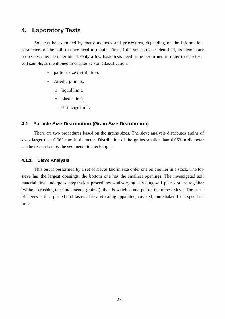
4. Laboratory Tests..................................................................................................................................... 27

4.1. Particle Size Distribution (Grain Size Distribution)......................................................... 27 4.1.1. Sieve Analysis ............................................................................................................................ 27 4.1.2. Sedimentation Technique (Hydrometer Analysis)...................................................................... 29

4.2. Atterberg Limits ................................................................................................................ 30 4.2.1. Shrinkage Limit .......................................................................................................................... 30 4.2.2. Plastic Limit................................................................................................................................ 30 4.2.3. Liquid Limit................................................................................................................................ 30 4.2.4. Derived limits ............................................................................................................................. 32

4.3. Other Commonly Determinated Soil Properties ............................................................... 33 4.3.1. Bulk density................................................................................................................................ 33 4.3.2. Specific weight ........................................................................................................................... 33 4.3.3. Wetness....................................................................................................................................... 33

4.4. Maximum Bulk Density ..................................................................................................... 34

4.5. Pure Compression (Unconfined Compression)................................................................. 35

4.6. Undrained Triaxial Test.................................................................................................... 37

PART TWO: Laboratory Research soil & fibre material, characterisations and tests ......................... 41

5. Laboratory Instrumentation.................................................................................................................. 42

6. Specimen Laboratory Testings .............................................................................................................. 44

6.1. Soil Specimen Elementary Characterisation..................................................................... 44

6.2. Standard Proctor Test....................................................................................................... 46

6.3. Pycnometer Test (Specific Weight) ................................................................................... 46

6.4. Grain Size Analysis ........................................................................................................... 47

6.5. Specimen Classification .................................................................................................... 50

6.6. Pure Compression............................................................................................................. 50

6.7. Triaxial Compression........................................................................................................ 53 6.7.1. Unreinforced Soil Testing........................................................................................................... 53 6.7.2. Reinforced Soil Testing .............................................................................................................. 55

6.7.2.1. Test I. 0.5% Reinforcement.................................................................................................. 57 6.7.2.2. Test III. 1% Reinforcement .................................................................................................. 61 6.7.2.3. Evaluation by Mohr’s Circle Diagram ................................................................................. 64

7. Conclusion ...............................................................................................................................................66

Bibliography ...................................................................................................................................................... 67

L IST OF FIGURES

Figure 2-1. Geotextile [13] ................................................................................................................................... 14

Figure 2-2. Geogrid[14] ....................................................................................................................................... 14

Figure 2-3. Geonet[15] ......................................................................................................................................... 14

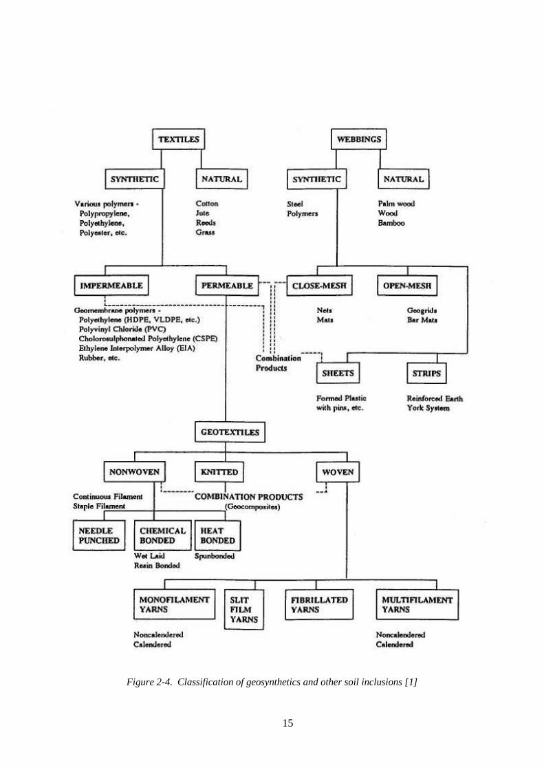
Figure 2-4. Classification of geosynthetics and other soil inclusions [1] ............................................................ 15

Figure 2-5. Polypropylene fibres „Geofibers“ by Synthetic Industries (USA) [4] ............................................... 18

Figure 2-6. Fibre „Texsol“ by Kordárna a.s. (Czech Republic), employed in the thesis [0].............................. 19

Figure 3-1. Sieve numbers [12]............................................................................................................................. 22

Figure 3-2. Unified Soil Classification System – ASTM D2488 [11] .................................................................... 23

Figure 3-3. Letter symbols for soil divisions [5] ................................................................................................... 24

Figure 3-4. Plasticity Chart for the Unified Soil Classification System [10]........................................................ 24

Figure 3-5. Soil classification diagram ČSN ISO 14688-2 [25] .......................................................................... 26

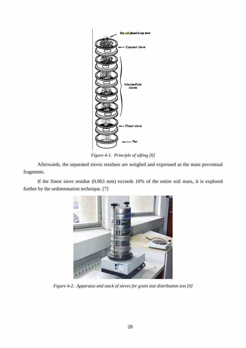
Figure 4-1. Principle of sifting [6] ....................................................................................................................... 28

Figure 4-2. Apparatus and stack of sieves for grain size distribution test [0] ..................................................... 28

Figure 4-3. Progress of particles sedimentation, performed on the thesis‘ sample [0] ....................................... 29

Figure 4-4. 3 mm diameter threads, test of plasticity on the thesis‘ sample [0] .................................................. 30

Figure 4-5. Cone penetrometer – apparatus for measuring the cone penetration [9] ......................................... 31

Figure 4-6. Cone standardised geometry and mass [9] ....................................................................................... 32

Figure 4-7. Pycnometer with boiling suspension in a sand bath [0].................................................................... 33

Figure 4-8. The Proctor mortar and rammer [0]................................................................................................. 34

Figure 4-9. Bulk density – moisture relationship, the Proctor test....................................................................... 35

Figure 4-10. Mould for remoulded specimen preparation [0] ............................................................................. 36

Figure 4-11. Stress-strain curve of a metal (Stress, kPa; strain, %) [18]............................................................ 37

Figure 4-12. Shear breaking plane, unconfined compression test of the thesis‘ sample [0]................................ 37

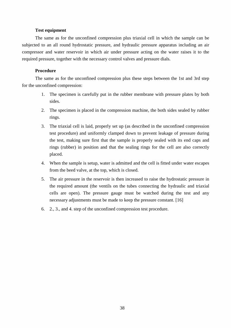
Figure 4-13. Specimen prepared for triaxial test [0] ........................................................................................... 39

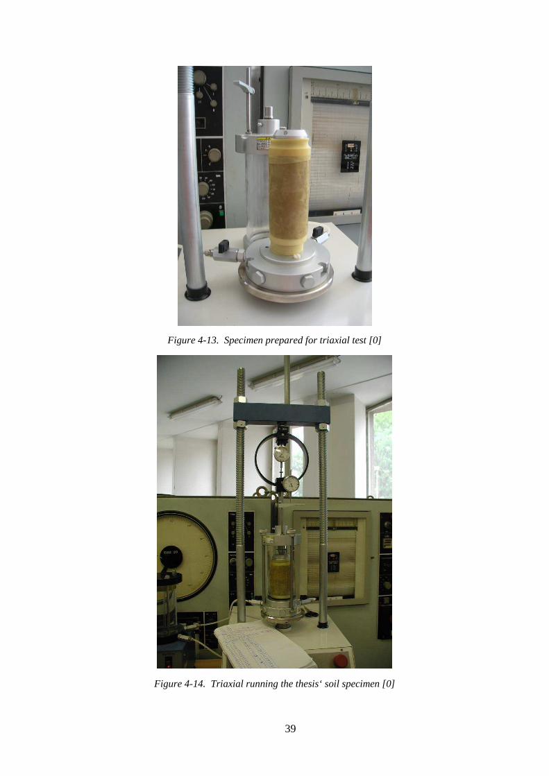
Figure 4-14. Triaxial running the thesis‘ soil specimen [0]................................................................................. 39

Figure 4-15. The Mohr circle [19] .......................................................................................................................40

Figure 4-16. Evaluation of the triaxial test [19] .................................................................................................. 40

Figure 5-1. Triaxial ELE Multiplex 50 [0]............................................................................................................ 42

Figure 5-2. Kern 600-2M [21] ............................................................................................................................. 43

Figure 5-3. Balance Kern DE60K20 [0] .............................................................................................................. 43

Figure 5-4. Oven Venticell 111 [0] .....................................................................................................................44

Figure 6-1. Determination of specimen density and wetness ............................................................................... 44

Figure 6-2. Data for determining liquidity limit................................................................................................... 45

Figure 6-3. Regressive curve for obtaining the liquidity limit.............................................................................. 45

Figure 6-4. Plastic limit data ............................................................................................................................... 45

Figure 6-5. Standard Proctor test data ................................................................................................................ 46

Figure 6-6. Regressive curve for determining the optimal wetness...................................................................... 46

Figure 6-7. Specific weight, measured data ......................................................................................................... 46

Figure 6-8. Temperature correction chart [7] ..................................................................................................... 47

Figure 6-9. Dynamic viscosity according to temperature [7] .............................................................................. 48

Figure 6-10. Dynamic viscosity – temperature relationship according to the table above.................................. 48

Figure 6-11. Sedimentation technique, input data ............................................................................................... 48

Figure 6-12. Hydrometer test, data measured and computed .............................................................................. 49

Figure 6-13. Grain size curve of the thesis‘ soil sample ...................................................................................... 49

Figure 6-14. Calibration chart for the measuring ring ........................................................................................ 51

Figure 6-15. Calibration curve for the measuring ring........................................................................................ 51

Figure 6-16. Pure compression test, data measured and computed..................................................................... 52

Figure 6-17. Pure compression test, stress-deformation curves .......................................................................... 53

Figure 6-18. Triaxial test of unreinforced soil, data measured and computed .................................................... 54

Figure 6-19. Triaxial test of unreinforced soil, stress-deformation curves .......................................................... 55

Figure 6-20. Widht extension of the fibres [24] ................................................................................................... 55

Figure 6-21. Mechanical property of the Texsol fibres [24] ................................................................................ 56

Figure 6-22. Mixture of soil and fibres [0] .......................................................................................................... 56

Figure 6-23. Triaxial test of 0.5% reinforced soil I, data measured and computed............................................. 58

Figure 6-24. Triaxial test of 0.5% reinforced soil, stress-deformation curves..................................................... 58

Figure 6-25. Reinforced specimens after triaxial test (1) unconfined (2) confined compression [0]................... 59

Figure 6-26. Shear breaking plane, reinforced specimen [0] ............................................................................... 59

Figure 6-27. Triaxial test of 0.5% reinforced soil II, data measured and computed ........................................... 60

Figure 6-28. Stress-deformation curves of reinforced and unreinforced triaxial-tested samples ........................ 61

Figure 6-29. Triaxial test of 1% reinforced soil, data measured and computed .................................................. 63

Figure 6-30. Stress-deformation curves, Test III (1% reinforcement) + unreinforced specimens ....................... 63

Figure 6-31. Stress-Strain Curves for Clay [3].................................................................................................... 64

Figure 6-32. Stress-Strain Curves for Sand [3] .................................................................................................... 64

12

PART ONE: Background

literature review, geotechnical terms & issues

13

1. Introduction

The use of inclusions to improve the mechanical properties of soils dates to ancient times.

However, it is only within the last quarter of century or so that analytical and experimental studies

have led to the contemporary soil reinforcement techniques. [2]

Soil reinforcement is now a highly attractive alternative for embankment and retaining wall

projects because of the economic benefits it offers in relation to conventional retaining structures.

Moreover, its acceptance has also been triggered by a number of technical factors, that include

aesthetics, reliability, simple construction techniques, good seismic performance, and the ability to

tolerate large deformations without structural distress. [2] This technology is also very useful in

terms of modern industrial world approach, which has introduced terms such as environment-

friendly, sustainable development, etc.

One of the most recent technologies discovered in the sphere of soil reinforcment is micro-

reinforcement by short thin plastic fibres. In this method, the fibres are evenly mixed in the soil, in

situ. The soil is then compacted layer by layer, as in usual procedures of ground improvement. The

fibres-reinforced soil is to have, reportedly, higher bearing capacity and slower, gradual settlement.

The thesis‘ conclusion should match this statement.

First, the issues of soil and soil reinforcement needs to be introduced.

14

2. Geosynthetics

2.1. Related Terms

Ground improvement or ground modification engineering is the collective term for any

mechanical, hydrological, physicochemical, biological methods or any combination of such

methods employed to improve certain properties of natural or man-made soil deposits.

The term reinforced soil refers to a soil strengthened by a material capable of resisting

tensile stresses and interacting with the soil through friction and/or adhesion.

A geosynthetic is defined as a planar product manufactured from a polymeric material used

with soil, rock, earth, or other geotechnical-related material as an integral part of a civil engineering

project, structure, or system. [1]

2.2. Definitions and Types

A geotextile (Figure 2-1) is a permeable geosynthetic made of textile materials. Geogrids

(Figure 2-2) are primarily used for reinforcement; they are formed by a regular network of tensile

elements with apertures of sufficient size to interlock with surrounding fill material. Geonets

(Figure 2-3) are formed by the continuous extrusion of polymeric ribs at acute angles to each other.

They have large openings in a netlike configuration and the primary function of geonets is drainage.

Geomembranes are low permeability geosynthetics used as fluid barriers. Geotextiles and related

products such as nets and grids can be combined with geomembranes and other synthetics to take

advantage of the best attributes of each component. These products are called geocomposites, and

they may be composites of geotextile-geonets, geotextile-geogrids, geotextile-geomembranes,

geomembrane-geonets, geotextile-polymeric cores, and even threedimensional polymeric cell

structures. There is almost no limit to the variety of geocomposites that are possible and useful. The

general generic term encompassing all these materials is geosynthetic. A convenient classification

system for geosynthetics is given in Figure 2-4. [1]

Figure 2-1. Geotextile [13]

Figure 2-2. Geogrid[14]

Figure 2-3. Geonet[15]

15

Figure 2-4. Classification of geosynthetics and other soil inclusions [1]

16

2.3. Manufacture

Most geosynthetics are made from synthetic polymers such as polypropylene, polyester,

polyethylene, polyamide, PVC, etc. These materials are highly resistant to biological and chemical

degradation.

In manufacturing geotextiles, elements such as fibres or yarns are combined into planar

textile structures. The fibres can be continuous filaments, which are very long thin strands of a

polymer, or staple fibres, which are short filaments, typically 20 to 100 mm long. The fibres may

also be produced by slitting an extruded plastic sheet or film to form thin flat tapes. In both

filaments and slit films, the extrusion or drawing process elongates the polymers in the direction of

the draw and increases the fibre strength.

Geotextile type is determined by the method used to combine the filaments or tapes into the

planar textile structure. The vast majority of geotextiles are either woven or nonwoven. Woven

geotextiles are made of monofilament, multifilament, or fibrillated yarns, or of slit films and tapes.

Although the weaving process is very old, nonwoven textile manufacture is a modem industrial

development. Synthetic polymer fibers or filaments are continuously extruded and spun, blown or

otherwise laid onto a moving belt. Then the mass of filaments or fibers are either needlepunched, in

which the filaments are mechanically entangled by a series of small needles, or heat bonded, in

which the fibers are welded together by heat and/or pressure at their points of contact in the

nonwoven mass.

Stiff geogrids with integral junctions are manufactured by extruding and orienting sheets of

polyolefins. Flexible geogrids are made of polyester yarns joined at the crossover points by knitting

or weaving, and coated with a polymer. [1]

2.4. Functions and Applications

Geosynthetics have six primary functions:

1. filtration,

2. drainage,

3. separation,

4. reinforcement,

5. fluid barrier,

6. protection.

Geosynthetic applications are usually defined by their primary, or principal function. In a

number of applications, in addition to the primary function, geosynthetics usually perform one or

17

more secondary functions. It is important to consider both the primary and secondary functions in

the design computations and specifications. [1]

2.5. Geosynthetics for Soil Reinforcement

The three primary applications soil reinforcement using geosynthetics are

1. reinforcing the base of embankments constructed on very soft foundations,

2. increasing the stability and steepness of slopes,

3. reducing the earth pressures behind retaining walls and abutments.

In the first two applications, geosynthetics permit construction that otherwise would be cost

prohibitive or technically not feasible. In the case of retaining walls, significant cost savings are

possible in comparison with conventional retaining wall construction. Other reinforcement and

stabilization applications in which geosynthetics have also proven to be very effective include roads

and railroads, large area stabilization, and natural slope reinforcement. [1]

2.6. Polypropylene Fibrillated Fibres

2.6.1. Method

Traditional methods of soil reinforcement involve the use of continuous planar inclusions

(e.g. metallic strips, geogrids, geotexiles) within earth structures. The inclusions provide tensile

resistance to the soil in a particular direction. Planes of weakness may be introduced along the

interface between reinforcement and soil. Short discrete fibers, if mixed uniformly within the soil

mass, can provide isotropic increase in the strength of the soil composite without introducing

continuous planes of weakness. Also, fiber-reinforcement solutions do not require design

considerations regarding anchorage as planar reinforcements do. The technique of fiber-

reinforcement has been increasingly adopted in geotechnical projects involving repair of failed

slope and stabilization of thin soil veneers. [4]

18

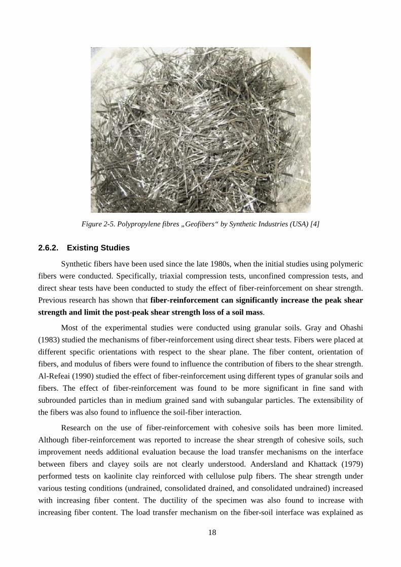
Figure 2-5. Polypropylene fibres „Geofibers“ by Synthetic Industries (USA) [4]

2.6.2. Existing Studies

Synthetic fibers have been used since the late 1980s, when the initial studies using polymeric

fibers were conducted. Specifically, triaxial compression tests, unconfined compression tests, and

direct shear tests have been conducted to study the effect of fiber-reinforcement on shear strength.

Previous research has shown that fiber-reinforcement can significantly increase the peak shear

strength and limit the post-peak shear strength loss of a soil mass.

Most of the experimental studies were conducted using granular soils. Gray and Ohashi

(1983) studied the mechanisms of fiber-reinforcement using direct shear tests. Fibers were placed at

different specific orientations with respect to the shear plane. The fiber content, orientation of

fibers, and modulus of fibers were found to influence the contribution of fibers to the shear strength.

Al-Refeai (1990) studied the effect of fiber-reinforcement using different types of granular soils and

fibers. The effect of fiber-reinforcement was found to be more significant in fine sand with

subrounded particles than in medium grained sand with subangular particles. The extensibility of

the fibers was also found to influence the soil-fiber interaction.

Research on the use of fiber-reinforcement with cohesive soils has been more limited.

Although fiber-reinforcement was reported to increase the shear strength of cohesive soils, such

improvement needs additional evaluation because the load transfer mechanisms on the interface

between fibers and clayey soils are not clearly understood. Andersland and Khattack (1979)

performed tests on kaolinite clay reinforced with cellulose pulp fibers. The shear strength under

various testing conditions (undrained, consolidated drained, and consolidated undrained) increased

with increasing fiber content. The ductility of the specimen was also found to increase with

increasing fiber content. The load transfer mechanism on the fiber-soil interface was explained as

19

an attraction between soil particles and fibers. Maher and Ho (1994) reported that randomly

distributed fibers increase the peak unconfined compressive strength, ductility, splitting tensile

strength and flexural toughness of kaolinite clay. The contribution of fiber-reinforcement was found

to be more significant for specimens with lower water contents.

While significant research has been conducted so far on the analysis and design of structures

with continuous planar reinforcement, the behavior of soils reinforced with randomly distributed

fibers needs additional evaluation. Past research has shown that the addition of fibers within soil

increases the peak shear strength and reduces the post-peak strength loss. [4]

2.6.3. Potential Applications

Fiber-reinforcement has been considered in projects involving

• slope stabilization,

• embankment construction,

• subgrade stabilization,

• stabilization of thin veneers such as landfill covers.

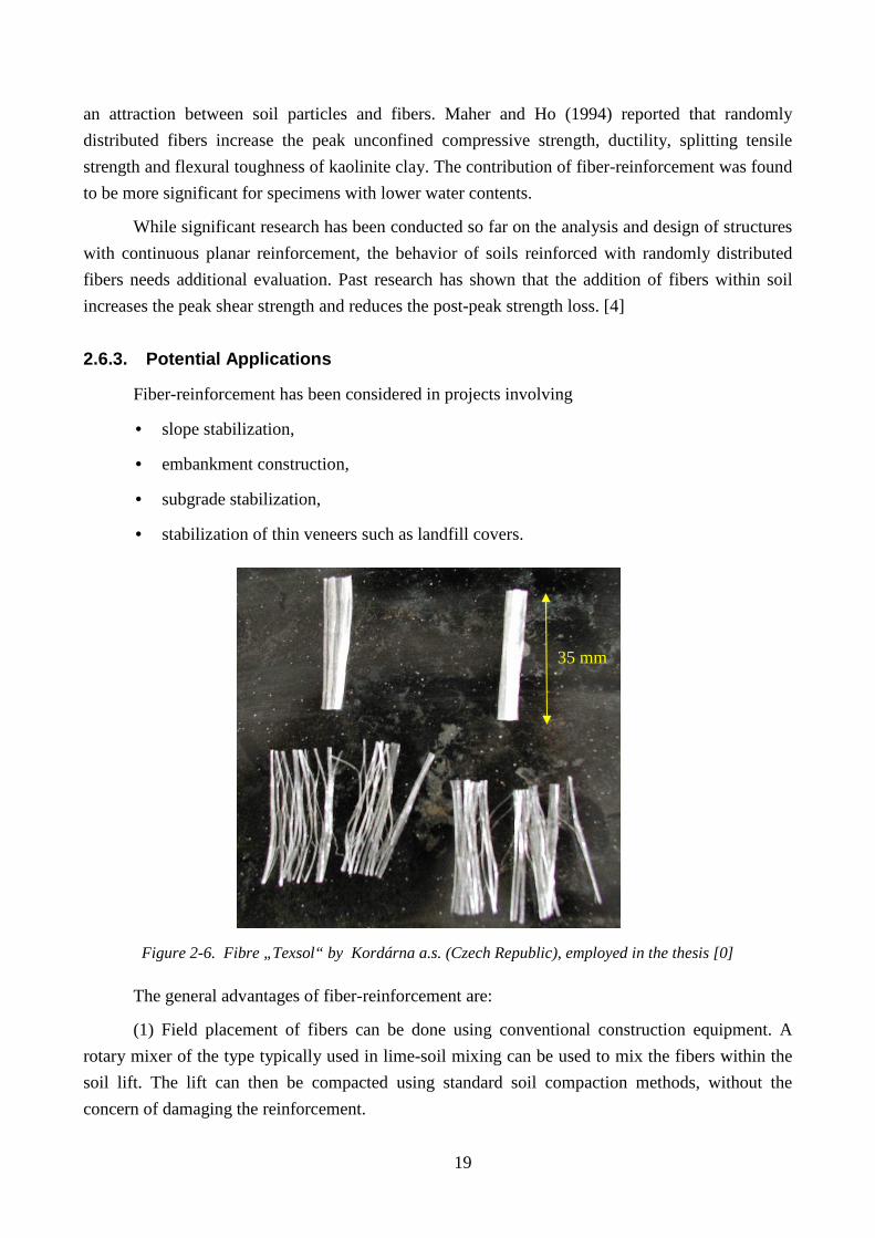
Figure 2-6. Fibre „Texsol“ by Kordárna a.s. (Czech Republic), employed in the thesis [0]

The general advantages of fiber-reinforcement are:

(1) Field placement of fibers can be done using conventional construction equipment. A

rotary mixer of the type typically used in lime-soil mixing can be used to mix the fibers within the

soil lift. The lift can then be compacted using standard soil compaction methods, without the

concern of damaging the reinforcement.

35 mm

20

(2) Unlike lime, cement and other chemical stabilization methods, the construction using

fiber-reinforcement is not significantly affected by weather conditions.

(3) The materials that can be used for fiber-reinforcement are widely available. Plant roots,

shredded tires, and recycled waste fibers can also be used as reinforcement in addition to factory-

manufactured synthetic fibers.

A promising application of fiber-reinforcement is in the localized repair of failed slopes. In

this case, the irregular shape of the soil “patches” limits the use of continuous planar reinforcement,

making the fiber-reinforcement an appealing alternative. Unlike planar reinforcement, fiber-

reinforcement does not require a large anchorage length, thus minimizing the excavation depth.

Another application is the stabilization of soil veneers (e.g. landfill covers) that are too steep

for stabilization using parallel-to-slope continuous reinforcements (Zornberg et al., 2001; Zornberg,

2005). Continuous horizontal reinforcement has been used, but this requires anchoring of the

reinforcement into competent material underlying the soil veneer. Also, parallel-to-slope

reinforcement requires anchoring the reinforcement at the slope crest. In contrast, the use of discrete

fibers does not require anchoring, and is economically and technically feasible.

In pavement construction, fiber-reinforcement can be used to stabilize a wide variety of

subgrade soils ranging from sand to high-plasticity clays (Santoni, et al., 2001; Grogan and

Johnson, 1993). The number of passes to failure in field road test was reported to increase by fiber-

reinforcement.

Fiber-reinforcement has also been used in combination with planar geosynthetics for

reinforced slopes or walls (Gregory, 1998). By increasing the shear strength of the backfill

materials, fiber reinforcement reduces the required amount of planar reinforcement and may

eliminate the need for secondary reinforcement. Fiber-reinforcement has been reported to be helpful

in eliminating the shallow failure on the slope face and reducing the cost of maintenance.

Fibers have also been reported to provide cracking control (Ziegler et al., 1998; Allan and

Kukacka, 1995). Earth structures constructed using clayey soils develop desiccation cracks when

subjected to wet-dry cycles. Fibers were found to effectively reduce the number and width of

desiccation cracks. Fiber reinforcement can also mitigate potential cracking induced by differential

settlements because fiber-reinforcement increases the ductility of the soil.

Fiber-reinforcement can also provide erosion control and facilitate vegetation development

since the compaction effort needed for fiber-reinforced soil is less than for unreinforced soil of

equivalent strength.

Fiber-reinforcement has also been used for stabilization of expansive soil (Puppala, 2000).

Fibers were found to reduce shrinkage and swell pressures of expansive clays.

The inclusion of fibers was also reported to improve the response of a soil mass subjected to

dynamic loading (Maher and Woods, 1990; Noorany and Uzdavines, 1989). [4]

21

2.7. Use of Micro-reinforcement Polypropylene Fibre s in the Czech Republic

Although the geosynthetics market and its product range in the Czech Republic is relatively

rich, no great mark of use occurs. The range of macro-reinforcement geosynthetics – geotextiles,

geogrids, geonets etc probably involves all the world-widely used elementary geosynthetics

products and methods.

There are some companies which produce geosynthetics for micro-reinforcement or work on

its research, namely Kordárna, a.s., of which fibres (Texsol) are employed for the research in this

thesis. Nevertheless, these geosynthetics still haven’t been evaluated enough to become a part of the

market with geosynthetics.

Phenomenon of the micro-reinforcement is at the beginning phase both in the world and the

Czech Republic, although there are considerably more studies researching the matter abroad

(especially in U. S. A.).

2.8. Conclusion

In less than 30 years, geosynthetics have revolutionized many aspects of our practice, and in

some applications they have entirely replaced the traditional construction material. In many cases,

the use of a geosynthetic can significantly increase the safety factor, improve performance, reduce

impact on environment, and reduce costs in comparison with conventional design and construction

alternatives. [1] However, reinforced soil with randomly distributed fibres as one of the reinforcing

techniques hasn’t been explored and evaluated enough, although it could have principal effect on

existing geotechnical engineering know-how.

3. Soil Classification

3.1. Objective

The principal objective of soil classification is the prediction of engineering properties and

behavior of a soil based on a few simple laboratory or field tests. The results of these tests are then

used to identify the soil and put it into a group of soils that have similar engineering characteristics.

[5] An important part of soil classification is the particle size distribution and the Atterberg limits

[6] (more in chapter 4: Laboratory Tests).

3.2. Method

Geotechnical engineering recognizes several systems of soil classification, e. g. the most

widely used systems in the United States are USCS (Unified Soil Classification System) –

22

internationally recognized system, AASHTO (American Association of State Highway and

Transportation Officials) Soil Classification System, Inorganic Soil Classification System – based

on plasticity, USDA (U. S. Department of Agriculture) Textural Soil Classification System, etc.

(more information in [6]). Classification system used in the Czech Republic is defined by a Czech

norm ČSN ISO 14688-2 (classification diagram p. 26).

Soils seldom exist in nature separately as sand, gravel, or any other single component. Soils

usually form mixtures with varying proportions of different size particles. Each component

contributes to the characteristics of the mixture. The USCS is based on the textural or plasticity-

compressibility characteristics that indicate how a soil will behave as a construction material. In the

USCS, all soils are divided into three major divisions:

(1) coarse grained, (2) fine grained, and (3) highly organic.

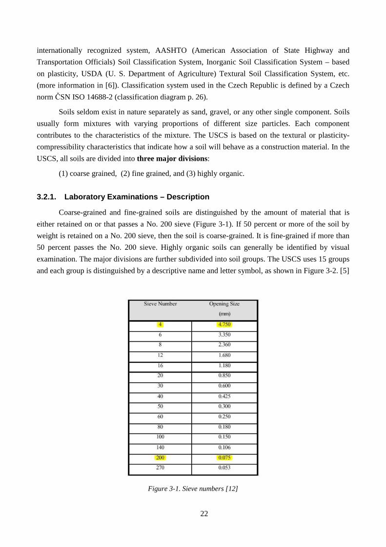
3.2.1. Laboratory Examinations – Description

Coarse-grained and fine-grained soils are distinguished by the amount of material that is

either retained on or that passes a No. 200 sieve (Figure 3-1). If 50 percent or more of the soil by

weight is retained on a No. 200 sieve, then the soil is coarse-grained. It is fine-grained if more than

50 percent passes the No. 200 sieve. Highly organic soils can generally be identified by visual

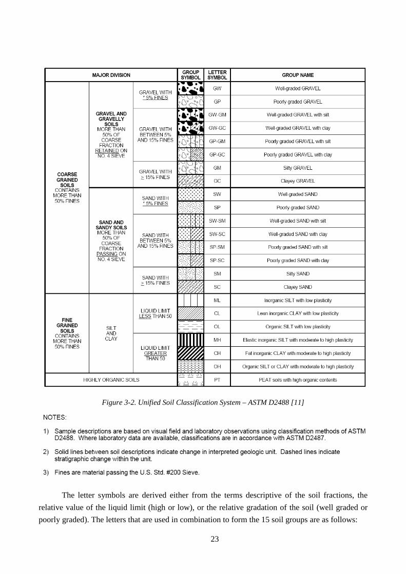
examination. The major divisions are further subdivided into soil groups. The USCS uses 15 groups

and each group is distinguished by a descriptive name and letter symbol, as shown in Figure 3-2. [5]

Figure 3-1. Sieve numbers [12]

23

Figure 3-2. Unified Soil Classification System – ASTM D2488 [11]

The letter symbols are derived either from the terms descriptive of the soil fractions, the

relative value of the liquid limit (high or low), or the relative gradation of the soil (well graded or

poorly graded). The letters that are used in combination to form the 15 soil groups are as follows:

24

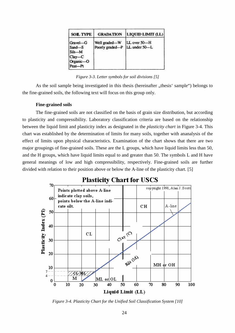
Figure 3-3. Letter symbols for soil divisions [5]

As the soil sample being investigated in this thesis (hereinafter „thesis‘ sample“) belongs to

the fine-grained soils, the following text will focus on this group only.

Fine-grained soils

The fine-grained soils are not classified on the basis of grain size distribution, but according

to plasticity and compressibility. Laboratory classification criteria are based on the relationship

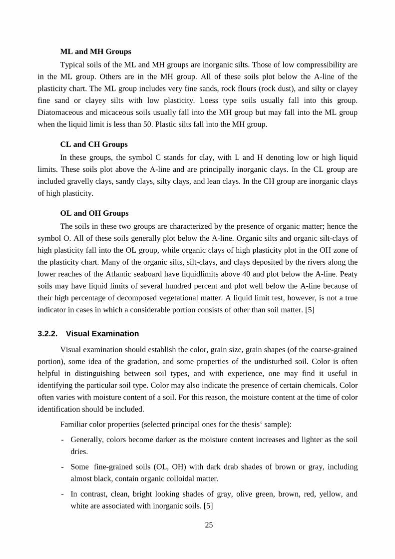
between the liquid limit and plasticity index as designated in the plasticity chart in Figure 3-4. This

chart was established by the determination of limits for many soils, together with ananalysis of the

effect of limits upon physical characteristics. Examination of the chart shows that there are two

major groupings of fine-grained soils. These are the L groups, which have liquid limits less than 50,

and the H groups, which have liquid limits equal to and greater than 50. The symbols L and H have

general meanings of low and high compressibility, respectively. Fine-grained soils are further

divided with relation to their position above or below the A-line of the plasticity chart. [5]

Figure 3-4. Plasticity Chart for the Unified Soil Classification System [10]

25

ML and MH Groups

Typical soils of the ML and MH groups are inorganic silts. Those of low compressibility are

in the ML group. Others are in the MH group. All of these soils plot below the A-line of the

plasticity chart. The ML group includes very fine sands, rock flours (rock dust), and silty or clayey

fine sand or clayey silts with low plasticity. Loess type soils usually fall into this group.

Diatomaceous and micaceous soils usually fall into the MH group but may fall into the ML group

when the liquid limit is less than 50. Plastic silts fall into the MH group.

CL and CH Groups

In these groups, the symbol C stands for clay, with L and H denoting low or high liquid

limits. These soils plot above the A-line and are principally inorganic clays. In the CL group are

included gravelly clays, sandy clays, silty clays, and lean clays. In the CH group are inorganic clays

of high plasticity.

OL and OH Groups

The soils in these two groups are characterized by the presence of organic matter; hence the

symbol O. All of these soils generally plot below the A-line. Organic silts and organic silt-clays of

high plasticity fall into the OL group, while organic clays of high plasticity plot in the OH zone of

the plasticity chart. Many of the organic silts, silt-clays, and clays deposited by the rivers along the

lower reaches of the Atlantic seaboard have liquidlimits above 40 and plot below the A-line. Peaty

soils may have liquid limits of several hundred percent and plot well below the A-line because of

their high percentage of decomposed vegetational matter. A liquid limit test, however, is not a true

indicator in cases in which a considerable portion consists of other than soil matter. [5]

3.2.2. Visual Examination

Visual examination should establish the color, grain size, grain shapes (of the coarse-grained

portion), some idea of the gradation, and some properties of the undisturbed soil. Color is often

helpful in distinguishing between soil types, and with experience, one may find it useful in

identifying the particular soil type. Color may also indicate the presence of certain chemicals. Color

often varies with moisture content of a soil. For this reason, the moisture content at the time of color

identification should be included.

Familiar color properties (selected principal ones for the thesis‘ sample):

- Generally, colors become darker as the moisture content increases and lighter as the soil

dries.

- Some fine-grained soils (OL, OH) with dark drab shades of brown or gray, including

almost black, contain organic colloidal matter.

- In contrast, clean, bright looking shades of gray, olive green, brown, red, yellow, and

white are associated with inorganic soils. [5]

26

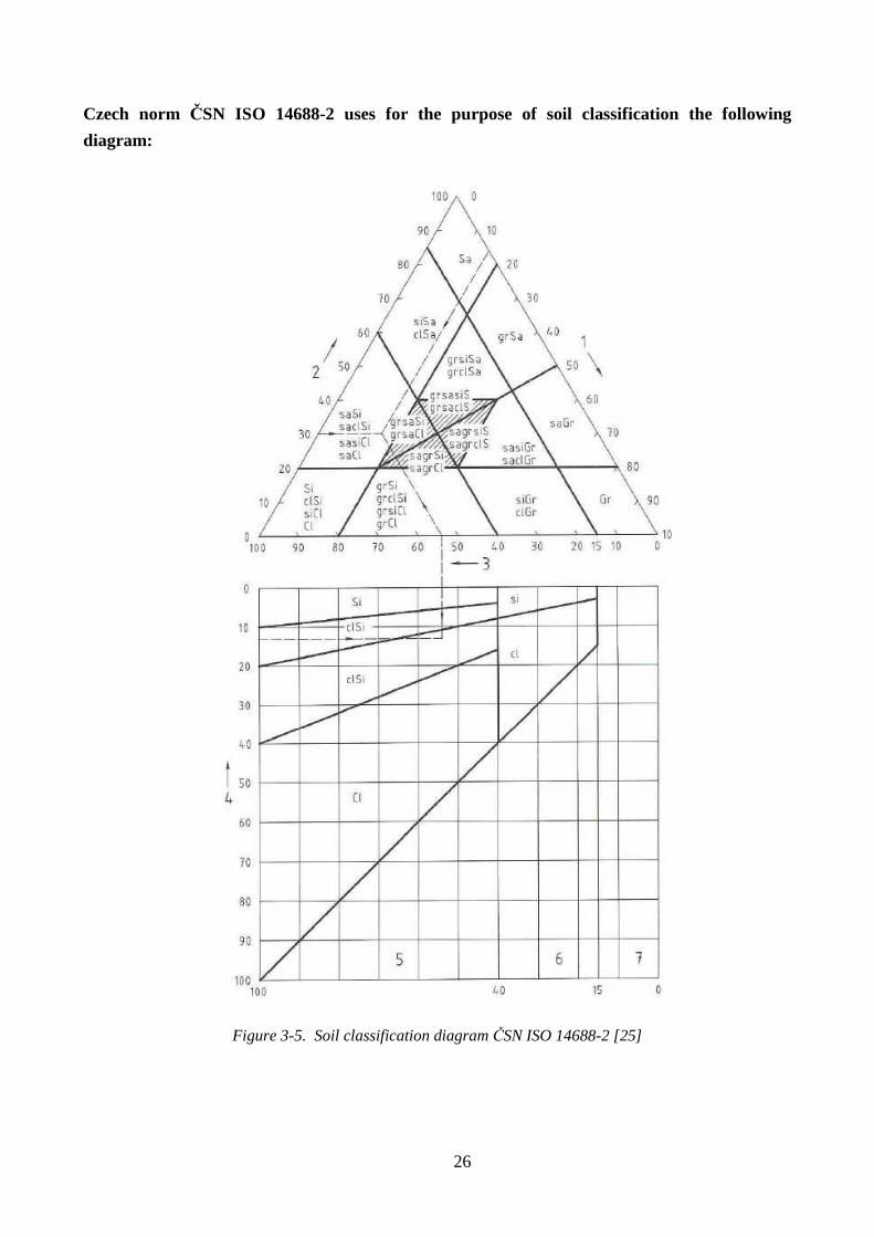
Czech norm ČSN ISO 14688-2 uses for the purpose of soil classification the following

diagram:

Figure 3-5. Soil classification diagram ČSN ISO 14688-2 [25]

27

4. Laboratory Tests

Soil can be examined by many methods and procedures, depending on the information,

parameters of the soil, that we need to obtain. First, if the soil is to be identified, its elementary

properties must be determined. Only a few basic tests need to be performed in order to classify a

soil sample, as mentioned in chapter 3: Soil Classification:

• particle size distribution,

• Atterberg limits,

o liquid limit,

o plastic limit,

o shrinkage limit.

4.1. Particle Size Distribution (Grain Size Distrib ution)

There are two procedures based on the grains sizes. The sieve analysis distributes grains of

sizes larger than 0.063 mm in diameter. Distribution of the grains smaller than 0.063 in diameter

can be researched by the sedimentation technique.

4.1.1. Sieve Analysis

This test is performed by a set of sieves laid in size order one on another in a stack. The top

sieve has the largest openings, the bottom one has the smallest openings. The investigated soil

material first undergoes preparation procedures – air-drying, dividing soil pieces stuck together

(without crushing the fundamental grains!), then is weighed and put on the uppest sieve. The stack

of sieves is then placed and fastened to a vibrating apparatus, covered, and shaked for a specified

time.

28

Figure 4-1. Principle of sifting [6]

Afterwards, the separated sieves residues are weighed and expressed as the mass percentual

fragments.

If the finest sieve residue (0.063 mm) exceeds 10% of the entire soil mass, it is explored

further by the sedimentation technique. [7]

Figure 4-2. Apparatus and stack of sieves for grain size distribution test [0]

29

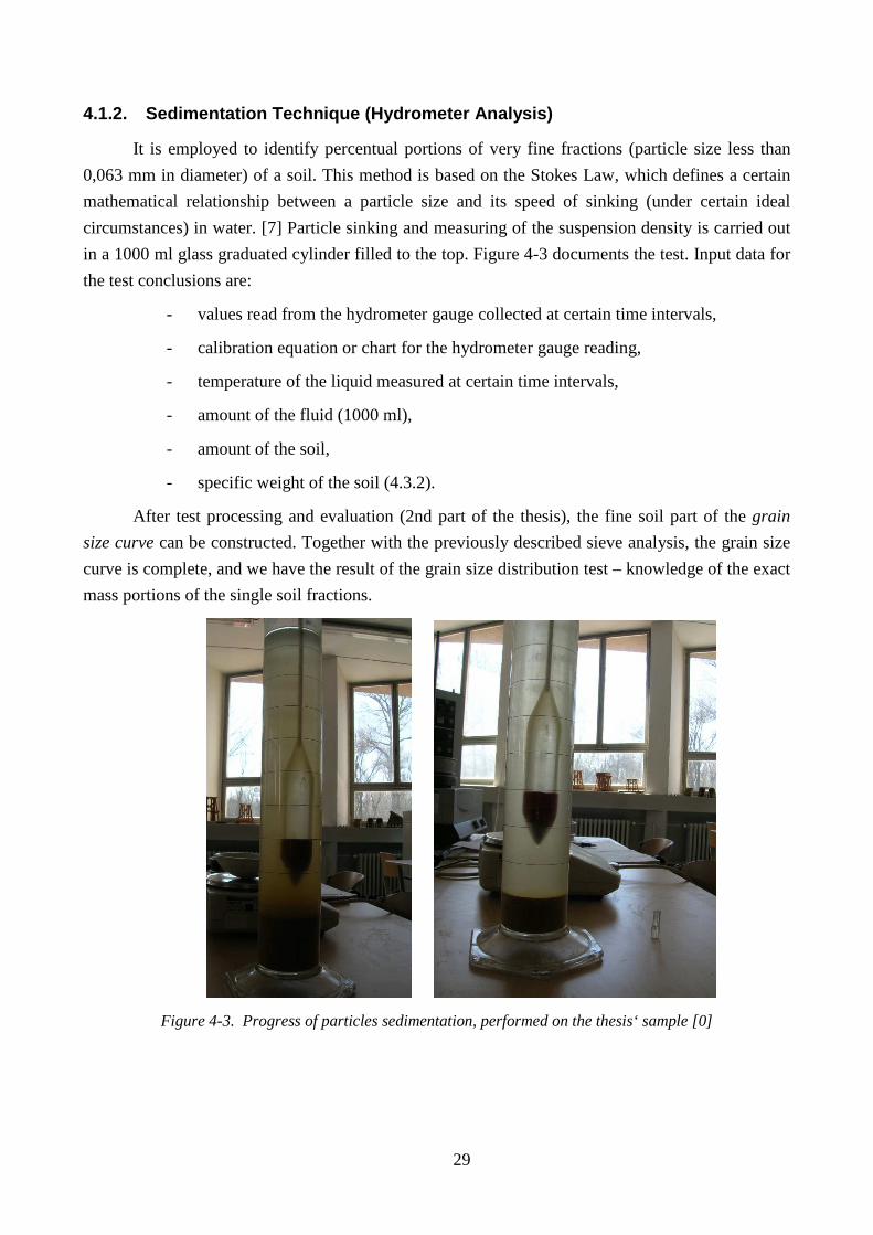
4.1.2. Sedimentation Technique (Hydrometer Analysis )

It is employed to identify percentual portions of very fine fractions (particle size less than

0,063 mm in diameter) of a soil. This method is based on the Stokes Law, which defines a certain

mathematical relationship between a particle size and its speed of sinking (under certain ideal

circumstances) in water. [7] Particle sinking and measuring of the suspension density is carried out

in a 1000 ml glass graduated cylinder filled to the top. Figure 4-3 documents the test. Input data for

the test conclusions are:

- values read from the hydrometer gauge collected at certain time intervals,

- calibration equation or chart for the hydrometer gauge reading,

- temperature of the liquid measured at certain time intervals,

- amount of the fluid (1000 ml),

- amount of the soil,

- specific weight of the soil (4.3.2).

After test processing and evaluation (2nd part of the thesis), the fine soil part of the grain

size curve can be constructed. Together with the previously described sieve analysis, the grain size

curve is complete, and we have the result of the grain size distribution test – knowledge of the exact

mass portions of the single soil fractions.

Figure 4-3. Progress of particles sedimentation, performed on the thesis‘ sample [0]

30

4.2. Atterberg Limits

The Atterberg limits are a basic measure of the nature of a fine-grained soil. Depending on

the water content of the soil, it may appear in four states: solid, semi-solid, plastic and liquid. In

each state the consistency and behavior of a soil is different and thus so are its engineering

properties. Thus, the boundary between each state can be defined based on a change in the soil's

behavior. The Atterberg limits can be used to distinguish between silt and clay. [8]

4.2.1. Shrinkage Limit

The shrinkage limit is the water content where further loss of moisture will not result in any

more volume reduction. The test to determine the shrinkage limit is ASTM International D427. The

shrinkage limit is much less commonly used than the liquid limit and the plastic limit.

The shrinkage limit is not utilized in this thesis.

4.2.2. Plastic Limit

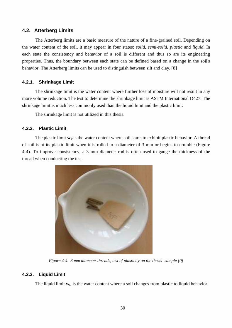
The plastic limit wP is the water content where soil starts to exhibit plastic behavior. A thread

of soil is at its plastic limit when it is rolled to a diameter of 3 mm or begins to crumble (Figure

4-4). To improve consistency, a 3 mm diameter rod is often used to gauge the thickness of the

thread when conducting the test.

Figure 4-4. 3 mm diameter threads, test of plasticity on the thesis‘ sample [0]

4.2.3. Liquid Limit

The liquid limit wL is the water content where a soil changes from plastic to liquid behavior.

31

Casagrande‘s method

Soil is placed into the metal cup portion of the device and a groove is made down its center

with a standardized tool. The cup is repeatedly dropped 10 mm onto a hard rubber base during

which the groove closes up gradually as a result of the impact. The number of blows for the groove

to close for 13 mm is recorded. The moisture content at which it takes 25 drops of the cup to cause

the groove to close is defined as the liquid limit.

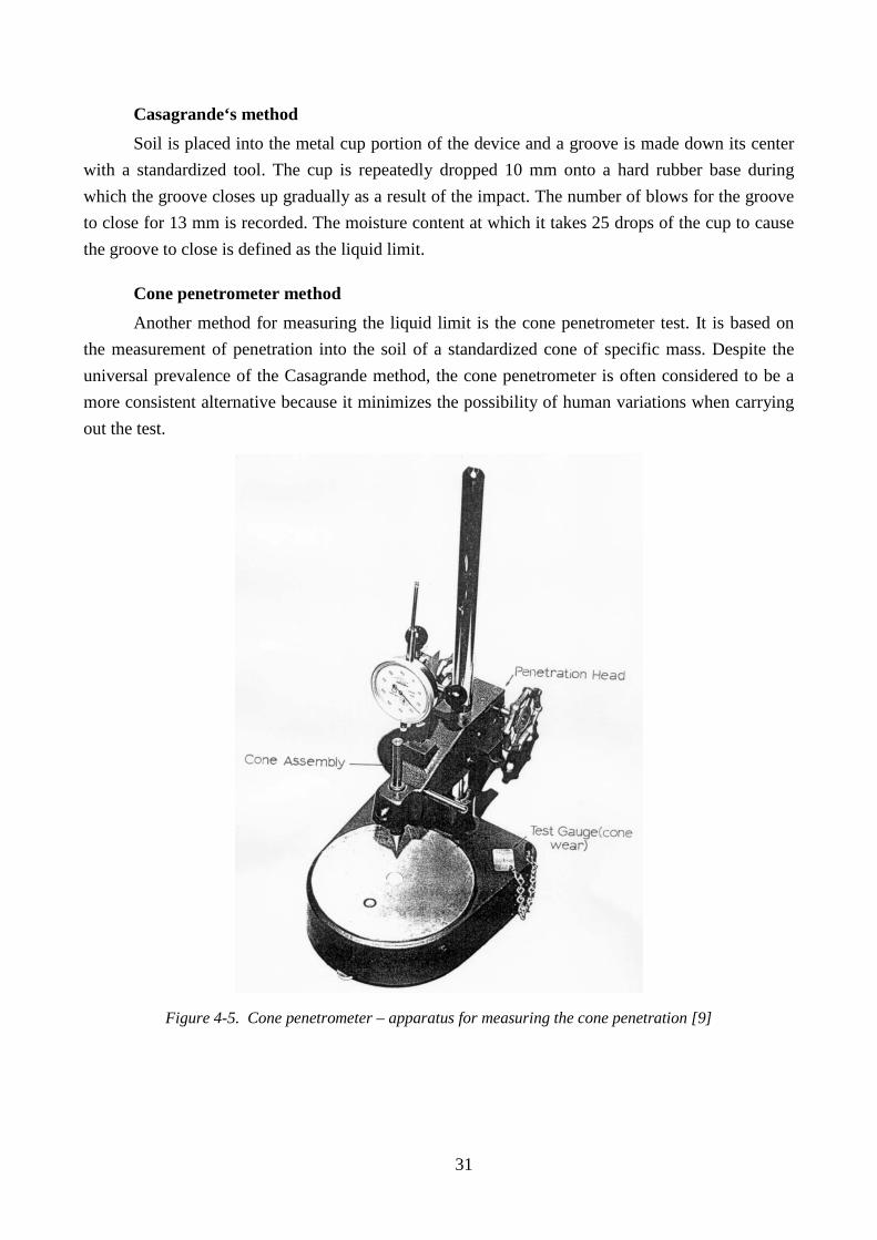
Cone penetrometer method

Another method for measuring the liquid limit is the cone penetrometer test. It is based on

the measurement of penetration into the soil of a standardized cone of specific mass. Despite the

universal prevalence of the Casagrande method, the cone penetrometer is often considered to be a

more consistent alternative because it minimizes the possibility of human variations when carrying

out the test.

Figure 4-5. Cone penetrometer – apparatus for measuring the cone penetration [9]

32

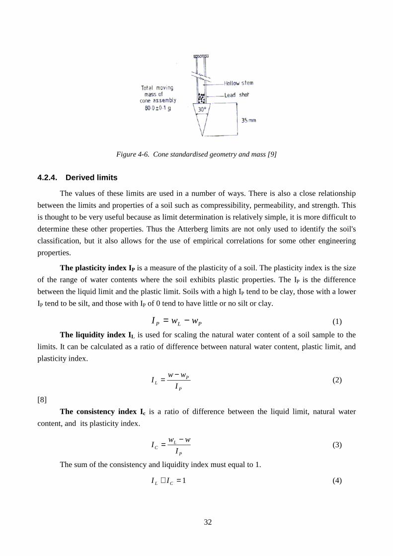
Figure 4-6. Cone standardised geometry and mass [9]

4.2.4. Derived limits

The values of these limits are used in a number of ways. There is also a close relationship

between the limits and properties of a soil such as compressibility, permeability, and strength. This

is thought to be very useful because as limit determination is relatively simple, it is more difficult to

determine these other properties. Thus the Atterberg limits are not only used to identify the soil's

classification, but it also allows for the use of empirical correlations for some other engineering

properties.

The plasticity index IP is a measure of the plasticity of a soil. The plasticity index is the size

of the range of water contents where the soil exhibits plastic properties. The IP is the difference

between the liquid limit and the plastic limit. Soils with a high IP tend to be clay, those with a lower

IP tend to be silt, and those with IP of 0 tend to have little or no silt or clay.

PLP wwI −= (1)

The liquidity index I L is used for scaling the natural water content of a soil sample to the

limits. It can be calculated as a ratio of difference between natural water content, plastic limit, and

plasticity index.

P

PL I

wwI

−= (2)

[8]

The consistency index Ic is a ratio of difference between the liquid limit, natural water

content, and its plasticity index.

P

LC I

wwI

−= (3)

The sum of the consistency and liquidity index must equal to 1.

1=+ CL II (4)

33

4.3. Other Commonly Determinated Soil Properties

4.3.1. Bulk density

The bulk density is a ratio between the mass and the volume of the soil.

V

m=ρ (5)

4.3.2. Specific weight

The specific weight is a ratio between the mass and the volume of the soil without pores.

s

ss V

m=ρ (6)

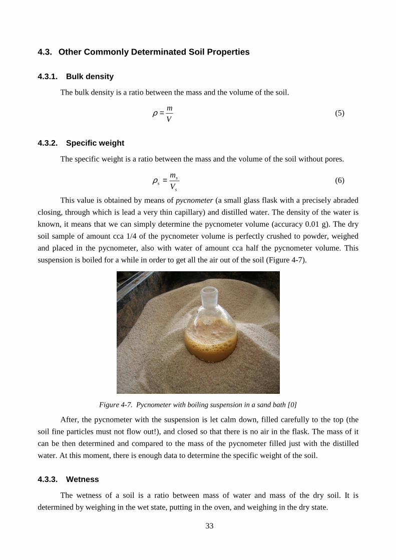
This value is obtained by means of pycnometer (a small glass flask with a precisely abraded

closing, through which is lead a very thin capillary) and distilled water. The density of the water is

known, it means that we can simply determine the pycnometer volume (accuracy 0.01 g). The dry

soil sample of amount cca 1/4 of the pycnometer volume is perfectly crushed to powder, weighed

and placed in the pycnometer, also with water of amount cca half the pycnometer volume. This

suspension is boiled for a while in order to get all the air out of the soil (Figure 4-7).

Figure 4-7. Pycnometer with boiling suspension in a sand bath [0]

After, the pycnometer with the suspension is let calm down, filled carefully to the top (the

soil fine particles must not flow out!), and closed so that there is no air in the flask. The mass of it

can be then determined and compared to the mass of the pycnometer filled just with the distilled

water. At this moment, there is enough data to determine the specific weight of the soil.

4.3.3. Wetness

The wetness of a soil is a ratio between mass of water and mass of the dry soil. It is

determined by weighing in the wet state, putting in the oven, and weighing in the dry state.

34

d

dw

m

mmw

−= (7)

4.4. Maximum Bulk Density

The maximum bulk density is a soil property depending on its moisture content. The soil can

be best compacted when it has the maximum bulk density (optimal moisture content), which is

utilized e. g. in construction of embankments.

The maximum bulk density is determined on the basis of experimental test, when a soil

sample is gradually dampened, consistently compacted and weighed. The soil reaches the maximum

density, when the sample reaches the highest mass (by sustaining the consistent volume at every

soil sample weighing). This procedure is called The Proctor test.

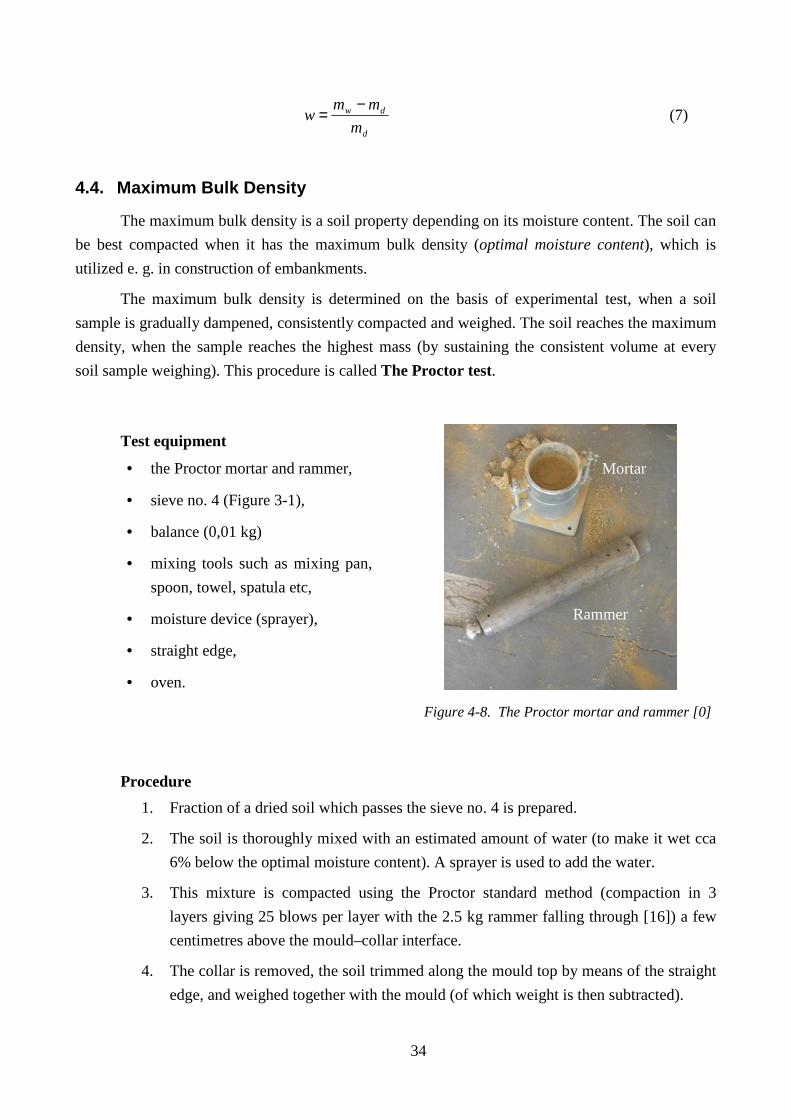
Test equipment

• the Proctor mortar and rammer,

• sieve no. 4 (Figure 3-1),

• balance (0,01 kg)

• mixing tools such as mixing pan,

spoon, towel, spatula etc,

• moisture device (sprayer),

• straight edge,

• oven.

Figure 4-8. The Proctor mortar and rammer [0]

Procedure

1. Fraction of a dried soil which passes the sieve no. 4 is prepared.

2. The soil is thoroughly mixed with an estimated amount of water (to make it wet cca

6% below the optimal moisture content). A sprayer is used to add the water.

3. This mixture is compacted using the Proctor standard method (compaction in 3

layers giving 25 blows per layer with the 2.5 kg rammer falling through [16]) a few

centimetres above the mould–collar interface.

4. The collar is removed, the soil trimmed along the mould top by means of the straight

edge, and weighed together with the mould (of which weight is then subtracted).

Mortar

Rammer

35

5. A sample of the soil is taken, weighed, and dried for later determination of the exact

wetness (%).

6. The steps above are repeated (the addition of water in step 2 is adequately less and

less, as it comes to the wanted moisture content!) until the soil mass starts to

diminish or stays constant.

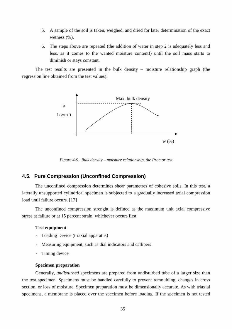
The test results are presented in the bulk density – moisture relationship graph (the

regression line obtained from the test values):

Figure 4-9. Bulk density – moisture relationship, the Proctor test

4.5. Pure Compression (Unconfined Compression)

The unconfined compression determines shear parametres of cohesive soils. In this test, a

laterally unsupported cylindrical specimen is subjected to a gradually increased axial compression

load until failure occurs. [17]

The unconfined compression strenght is defined as the maximum unit axial compressive

stress at failure or at 15 percent strain, whichever occurs first.

Test equipment

- Loading Device (triaxial apparatus)

- Measuring equipment, such as dial indicators and callipers

- Timing device

Specimen preparation

Generally, undisturbed specimens are prepared from undisturbed tube of a larger size than

the test specimen. Specimens must be handled carefully to prevent remoulding, changes in cross

section, or loss of moisture. Specimen preparation must be dimensionally accurate. As with triaxial

specimens, a membrane is placed over the specimen before loading. If the specimen is not tested

ρ

(kg/m3)

w (%)

Max. bulk density

36

immediately after preparation, precautions must be taken to prevent drying and consequent

development of capillary stresses.

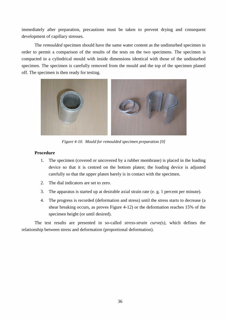
The remoulded specimen should have the same water content as the undisturbed specimen in

order to permit a comparison of the results of the tests on the two specimens. The specimen is

compacted in a cylindrical mould with inside dimensions identical with those of the undisturbed

specimen. The specimen is carefully removed from the mould and the top of the specimen planed

off. The specimen is then ready for testing.

Figure 4-10. Mould for remoulded specimen preparation [0]

Procedure

1. The specimen (covered or uncovered by a rubber membrane) is placed in the loading

device so that it is centred on the bottom platen; the loading device is adjusted

carefully so that the upper platen barely is in contact with the specimen.

2. The dial indicators are set to zero.

3. The apparatus is started up at desirable axial strain rate (e. g. 1 percent per minute).

4. The progress is recorded (deformation and stress) until the stress starts to decrease (a

shear breaking occurs, as proves Figure 4-12) or the deformation reaches 15% of the

specimen height (or until desired).

The test results are presented in so-called stress-strain curve(s), which defines the

relationship between stress and deformation (proportional deformation).

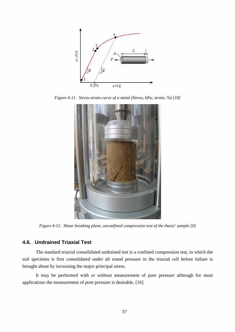
37

Figure 4-11. Stress-strain curve of a metal (Stress, kPa; strain, %) [18]

Figure 4-12. Shear breaking plane, unconfined compression test of the thesis‘ sample [0]

4.6. Undrained Triaxial Test

The standard triaxial consolidated undrained test is a confined compression test, in which the

soil specimen is first consolidated under all round pressure in the triaxial cell before failure is

brought about by increasing the major principal stress.

It may be performed with or without measurement of pore pressure although for most

applications the measurement of pore pressure is desirable. [16]

38

Test equipment

The same as for the unconfined compression plus triaxial cell in which the sample can be

subjected to an all round hydrostatic pressure, and hydraulic pressure apparatus including an air

compressor and water reservoir in which air under pressure acting on the water raises it to the

required pressure, together with the necessary control valves and pressure dials.

Procedure

The same as for the unconfined compression plus these steps between the 1st and 3rd step

for the unconfined compression:

1. The specimen is carefully put in the rubber membrane with pressure plates by both

sides.

2. The specimen is placed in the compression machine, the both sides sealed by rubber

rings.

3. The triaxial cell is laid, properly set up (as described in the unconfined compression

test procedure) and uniformly clamped down to prevent leakage of pressure during

the test, making sure first that the sample is properly sealed with its end caps and

rings (rubber) in position and that the sealing rings for the cell are also correctly

placed.

4. When the sample is setup, water is admitted and the cell is fitted under water escapes

from the beed valve, at the top, which is closed.

5. The air pressure in the reservoir is then increased to raise the hydrostatic pressure in

the required amount (the ventils on the tubes connecting the hydraulic and triaxial

cells are open). The pressure gauge must be watched during the test and any

necessary adjustments must be made to keep the pressure constant. [16]

6. 2., 3., and 4. step of the unconfined compression test procedure.

39

Figure 4-13. Specimen prepared for triaxial test [0]

Figure 4-14. Triaxial running the thesis‘ soil specimen [0]

40

The test results are similar to the previously described, with the difference of the side

pressure.

The strain and corresponding stress is plotted with stress abscissa and curve is drawn. The

maximum compressive stress at failure and the corresponding strain and cell pressure are found out.

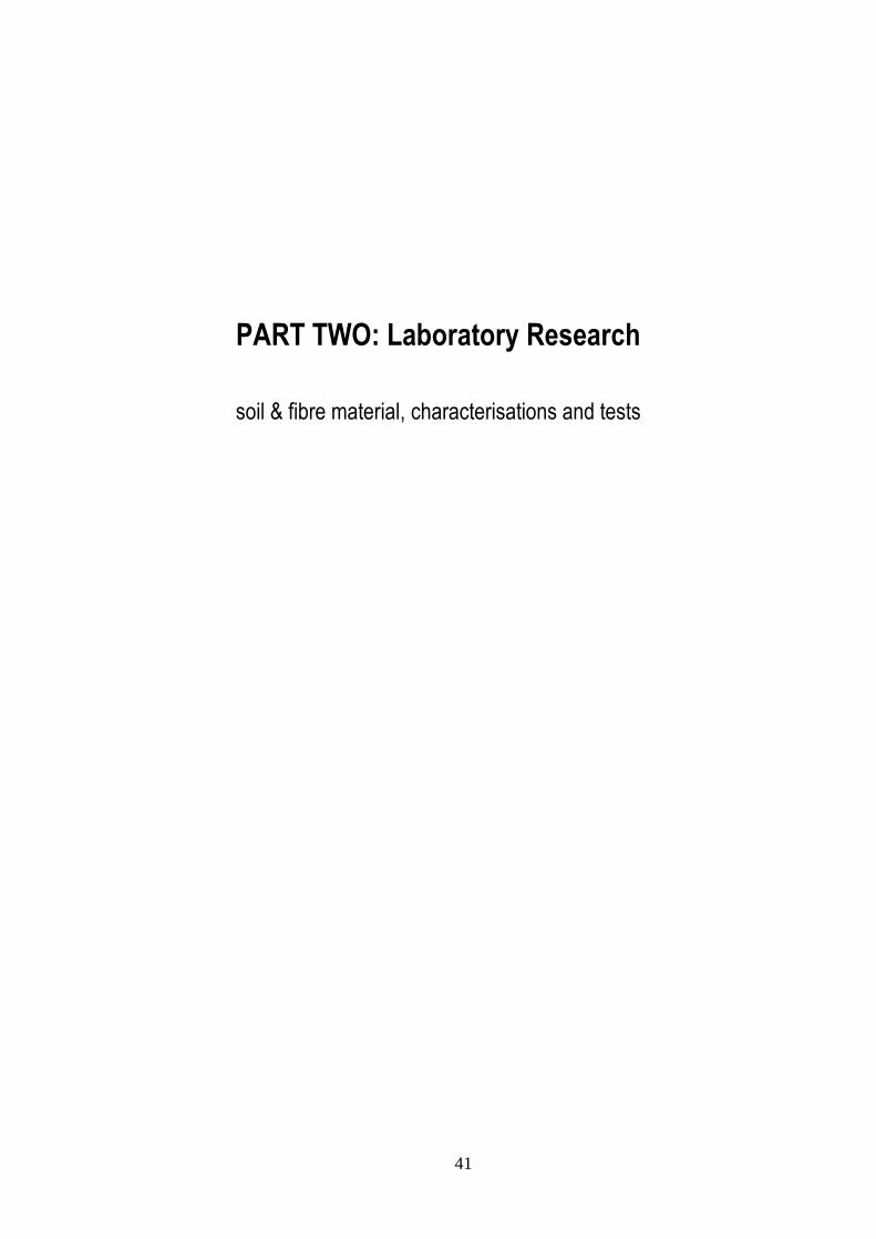
The stress results of the series of triaxial tests at increasing cell pressure are plotted on a

mohr stress diagram. In this diagram a semicircle is plotted with normal stress and abscissa shear

stress as ordinate.

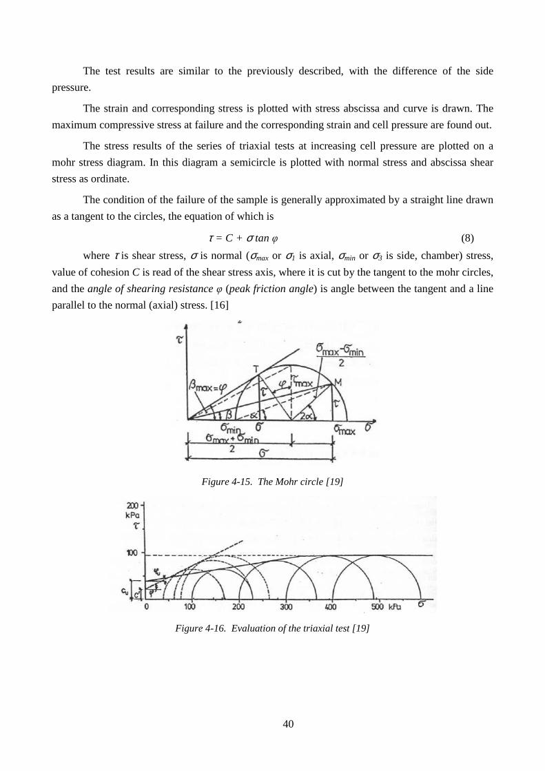
The condition of the failure of the sample is generally approximated by a straight line drawn

as a tangent to the circles, the equation of which is

τ = C + σ tan φ (8)

where τ is shear stress, σ is normal (σmax or σ1 is axial, σmin or σ3 is side, chamber) stress,

value of cohesion C is read of the shear stress axis, where it is cut by the tangent to the mohr circles,

and the angle of shearing resistance φ (peak friction angle) is angle between the tangent and a line

parallel to the normal (axial) stress. [16]

Figure 4-15. The Mohr circle [19]

Figure 4-16. Evaluation of the triaxial test [19]

41

PART TWO: Laboratory Research

soil & fibre material, characterisations and tests

42

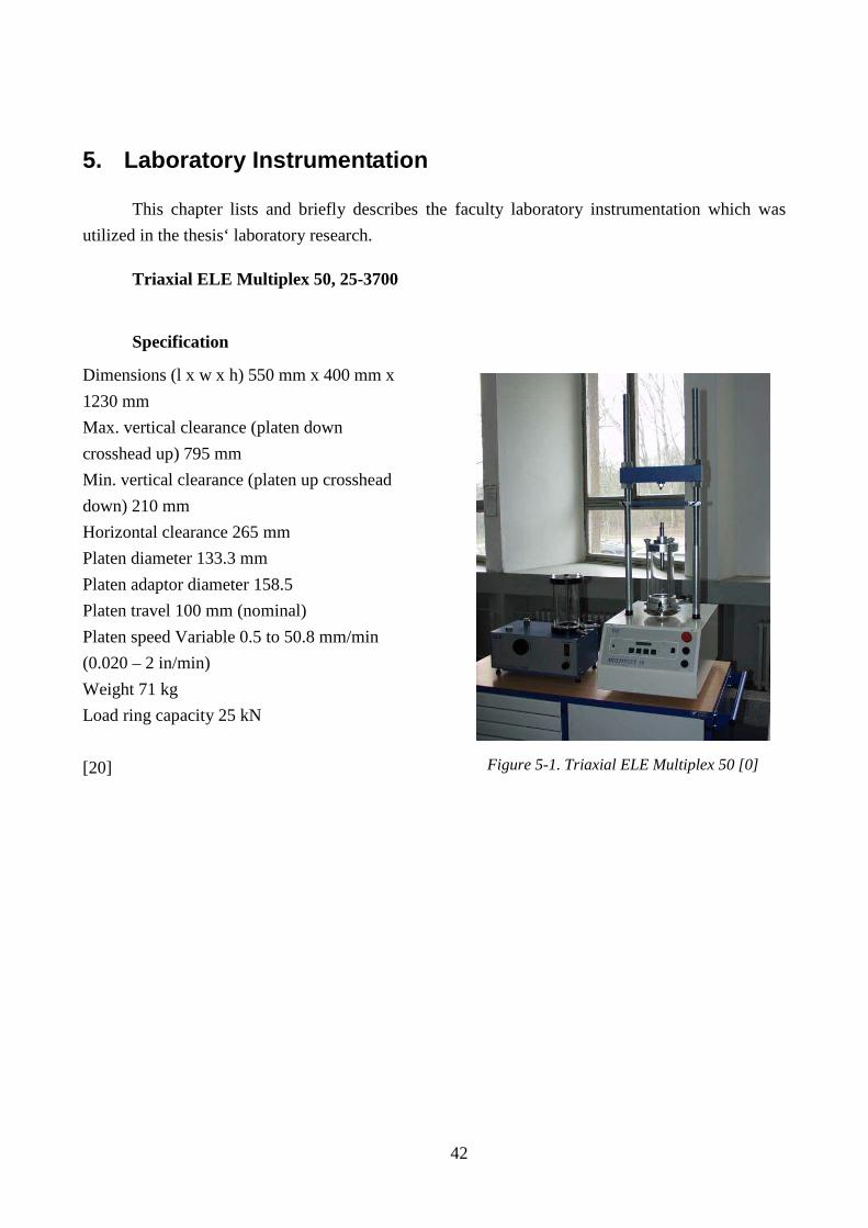
5. Laboratory Instrumentation

This chapter lists and briefly describes the faculty laboratory instrumentation which was

utilized in the thesis‘ laboratory research.

Triaxial ELE Multiplex 50, 25-3700

Specification

Dimensions (l x w x h) 550 mm x 400 mm x

1230 mm

Max. vertical clearance (platen down

crosshead up) 795 mm

Min. vertical clearance (platen up crosshead

down) 210 mm

Horizontal clearance 265 mm

Platen diameter 133.3 mm

Platen adaptor diameter 158.5

Platen travel 100 mm (nominal)

Platen speed Variable 0.5 to 50.8 mm/min

(0.020 – 2 in/min)

Weight 71 kg

Load ring capacity 25 kN

[20]

Figure 5-1. Triaxial ELE Multiplex 50 [0]

43

Balance Kern 600-2M

Accuracy: 0.01 g.

Capacity: 600 g.

[21]

Figure 5-2. Kern 600-2M [21]

Figure 5-3. Balance Kern DE60K20 [0]

Balance Kern DE60K20

• PLATFORM BALANCE, 60.0KG

• Resolution, weight:20g

• Weight, load max:60kg

• Accuracy, + percentage:20%

• IP rating:54

• Length / Height, external:310mm

• Range:60kg

• Weight, calibration:60kg

[22]

44

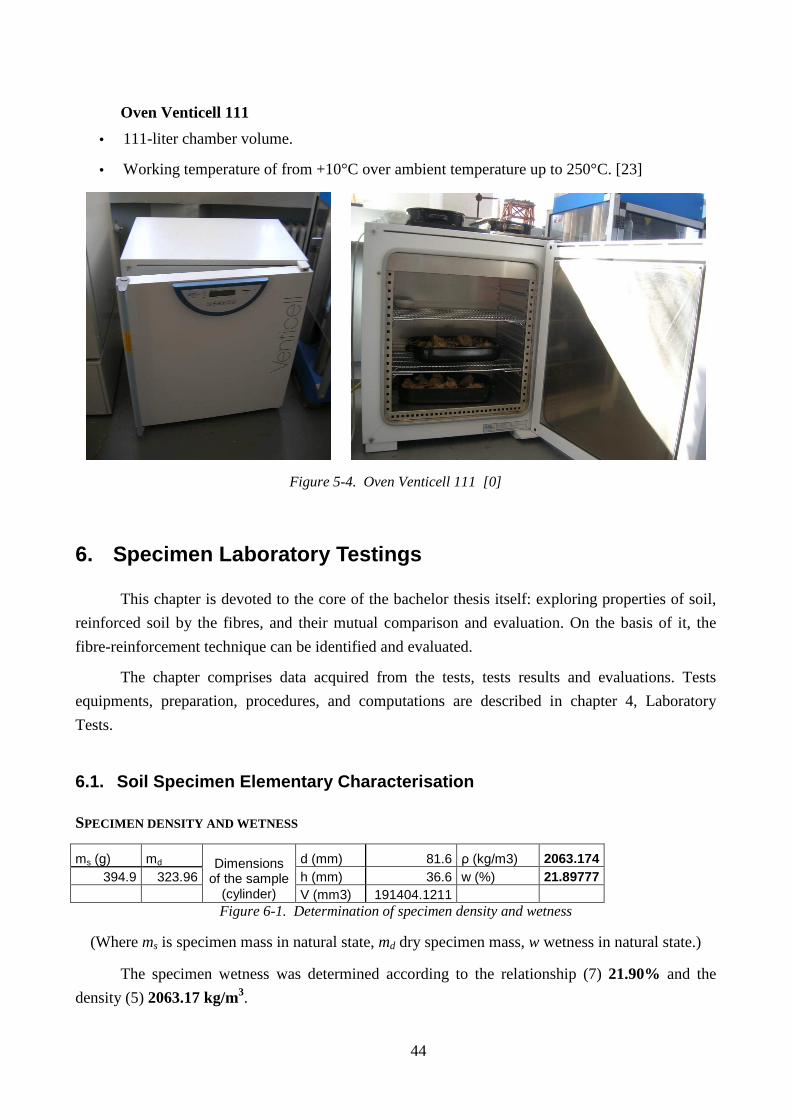
Oven Venticell 111

• 111-liter chamber volume.

• Working temperature of from +10°C over ambient temperature up to 250°C. [23]

Figure 5-4. Oven Venticell 111 [0]

6. Specimen Laboratory Testings

This chapter is devoted to the core of the bachelor thesis itself: exploring properties of soil,

reinforced soil by the fibres, and their mutual comparison and evaluation. On the basis of it, the

fibre-reinforcement technique can be identified and evaluated.

The chapter comprises data acquired from the tests, tests results and evaluations. Tests

equipments, preparation, procedures, and computations are described in chapter 4, Laboratory

Tests.

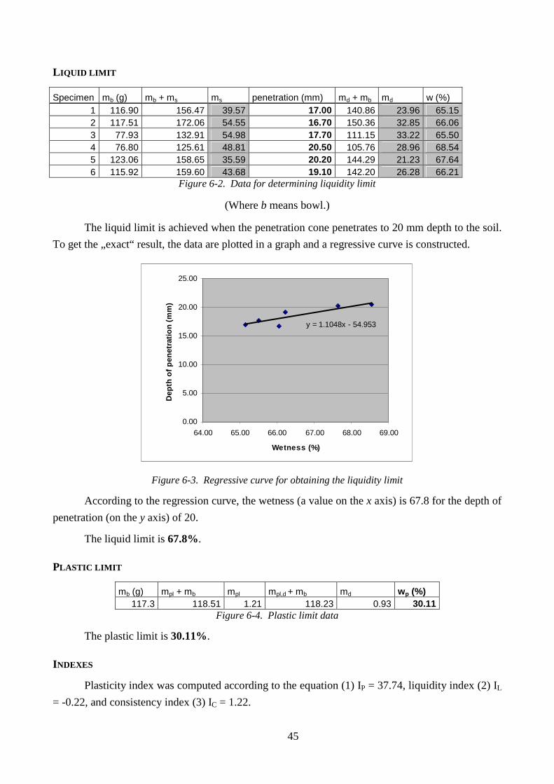
6.1. Soil Specimen Elementary Characterisation

SPECIMEN DENSITY AND WETNESS

ms (g) md d (mm) 81.6 ρ (kg/m3) 2063.174 394.9 323.96 h (mm) 36.6 w (%) 21.89777

Dimensions of the sample

(cylinder) V (mm3) 191404.1211 Figure 6-1. Determination of specimen density and wetness

(Where ms is specimen mass in natural state, md dry specimen mass, w wetness in natural state.)

The specimen wetness was determined according to the relationship (7) 21.90% and the

density (5) 2063.17 kg/m3.

45

L IQUID LIMIT

Specimen mb (g) mb + ms ms penetration (mm) md + mb md w (%) 1 116.90 156.47 39.57 17.00 140.86 23.96 65.15 2 117.51 172.06 54.55 16.70 150.36 32.85 66.06 3 77.93 132.91 54.98 17.70 111.15 33.22 65.50 4 76.80 125.61 48.81 20.50 105.76 28.96 68.54 5 123.06 158.65 35.59 20.20 144.29 21.23 67.64 6 115.92 159.60 43.68 19.10 142.20 26.28 66.21

Figure 6-2. Data for determining liquidity limit

(Where b means bowl.)

The liquid limit is achieved when the penetration cone penetrates to 20 mm depth to the soil.

To get the „exact“ result, the data are plotted in a graph and a regressive curve is constructed.

y = 1.1048x - 54.953

0.00

5.00

10.00

15.00

20.00

25.00

64.00 65.00 66.00 67.00 68.00 69.00

Wetness (%)

Dep

th o

f pen

etra

tion

(mm

)

Figure 6-3. Regressive curve for obtaining the liquidity limit

According to the regression curve, the wetness (a value on the x axis) is 67.8 for the depth of

penetration (on the y axis) of 20.

The liquid limit is 67.8%.

PLASTIC LIMIT

mb (g) mpl + mb mpl mpl,d + mb md wp (%) 117.3 118.51 1.21 118.23 0.93 30.11

Figure 6-4. Plastic limit data

The plastic limit is 30.11%.

INDEXES

Plasticity index was computed according to the equation (1) IP = 37.74, liquidity index (2) IL

= -0.22, and consistency index (3) IC = 1.22.

46

6.2. Standard Proctor Test

mortar mortar + soil soil bowl bowl + soil soil bowl + dry soil dry soil wetness

density (ρ)

kg kg kg g g g g g % kg/m3 4.30 6.00 1.70 111.70 320.60 208.90 284.94 173.24 20.58 1812.12 4.30 6.06 1.76 110.68 246.25 135.57 218.40 107.72 25.85 1876.08 4.30 6.10 1.80 111.95 222.04 110.09 197.02 85.07 29.41 1918.72 4.30 6.04 1.74 107.05 327.69 220.64 273.31 166.26 32.71 1854.76

Figure 6-5. Standard Proctor test data

The wetness is computed according to (7).

Likewise in the liquid limit test, there was a need to construct the regressive curve in order to

read the maximum density value.

Density - wetness relationship graph

1918.72

y = -0.3763x3 + 28.529x2 - 701.37x + 7443.9

1800.00

1820.00

1840.00

1860.00

1880.00

1900.00

1920.00

1940.00

19.00 24.00 29.00 34.00

Wetness (%)

Den

sity

(kg

/m3)

Figure 6-6. Regressive curve for determining the optimal wetness

The regressive curve indicates that the x for y maximum equals 29.41% (the highest y value

is identical to the value in the table above).

6.3. Pycnometer Test (Specific Weight)

boiled →

mpyc mpyc+water mwater mpyc+dry soil mdry soil mpyc+soil+water msoil+water msoil+water-soil 53.89 151.12 97.23 82.13 28.24 168.68 114.79 86.55

Figure 6-7. Specific weight, measured data

Input data Relationships (based on (5) and (6))

ρwater (g/cm3) 1

Vpyc (cm3) 97.23

Vsoil (cm3) 10.68

water

waterpyc

mV

ρ=

water

watersoil

mmV

ρsoil-water+soil−

=

47

mspecif (g/cm3) = 2.64

The specific weight of the specimen is 2.64 g/cm3.

6.4. Grain Size Analysis

The soil sample was of very fine clayey fractions, therefore the sedimentation technique of

the grain size analysis was employed. The following equations describes the unique empirical

relationships among the velocity of particles, which vary in sizes, sedimentation, hydrometer gauge

reading and calibration, temperature of the suspension and its density, etc.

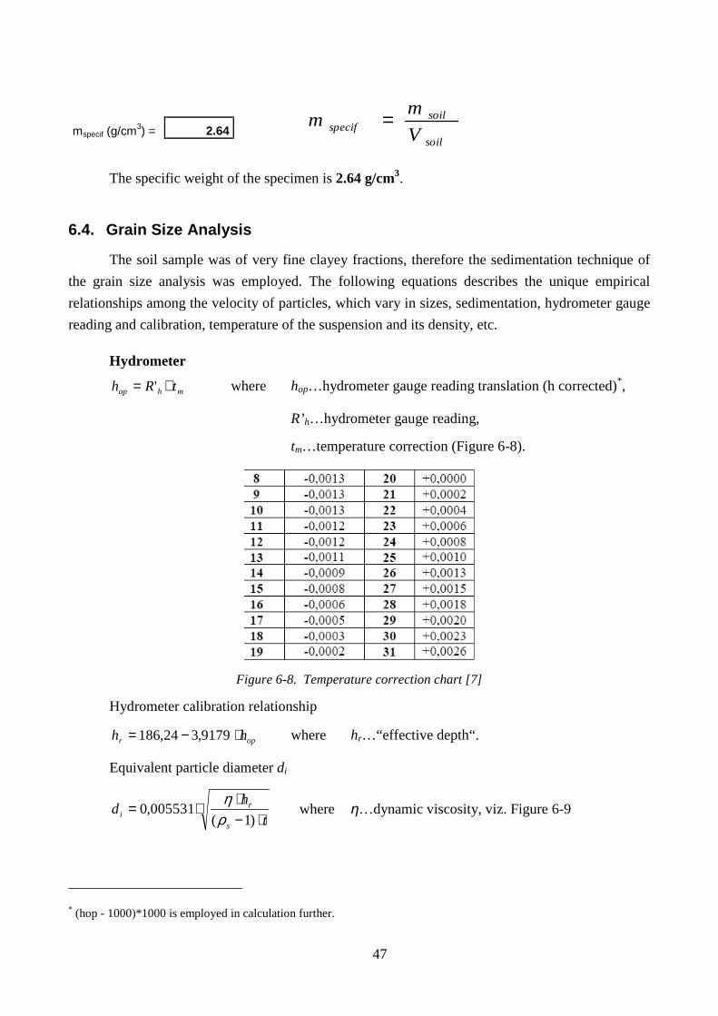
Hydrometer

mhop tRh += ' where hop…hydrometer gauge reading translation (h corrected)*,

R’h…hydrometer gauge reading,

tm…temperature correction (Figure 6-8).

Figure 6-8. Temperature correction chart [7]

Hydrometer calibration relationship

opr hh ⋅−= 9179,324,186 where hr…“effective depth“.

Equivalent particle diameter di

t

hd

s

ri ⋅−

⋅⋅=

)1(005531,0

ρη

where η…dynamic viscosity, viz. Figure 6-9

* (hop - 1000)*1000 is employed in calculation further.

soil

soilspecif V

mm =

48

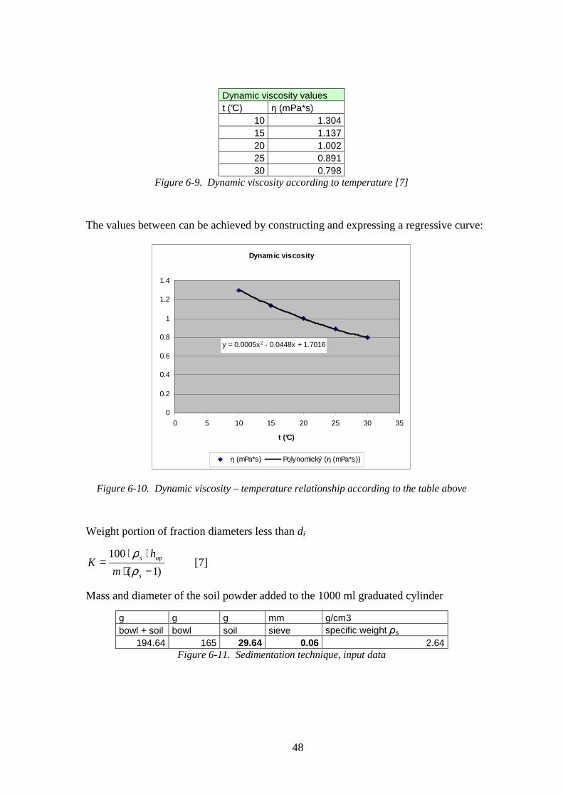
Dynamic viscosity values t (°C) η (mPa*s)

10 1.304 15 1.137 20 1.002 25 0.891 30 0.798

Figure 6-9. Dynamic viscosity according to temperature [7]

The values between can be achieved by constructing and expressing a regressive curve:

Dynamic viscosity

y = 0.0005x2 - 0.0448x + 1.7016

0

0.2

0.4

0.6

0.8

1

1.2

1.4

0 5 10 15 20 25 30 35

t (°C)

η (mPa*s) Polynomický (η (mPa*s))

Figure 6-10. Dynamic viscosity – temperature relationship according to the table above

Weight portion of fraction diameters less than di

)1(

100

−⋅⋅⋅

=s

ops

m

hK

ρρ

[7]

Mass and diameter of the soil powder added to the 1000 ml graduated cylinder

g g g mm g/cm3 bowl + soil bowl soil sieve specific weight ρs

194.64 165 29.64 0.06 2.64 Figure 6-11. Sedimentation technique, input data

49

Test progress data

time (min) time (s) R'h t (°C) hop hr η d i (mm) K (%) (hop supplied) 5 1.0178 21.93 1.0182 182.2508 0.9596 0.0255 98.6732 18.1860 10 1.0176 21.93 1.0180 182.2516 0.9596 0.0180 97.5880 17.9860 30 1.0174 21.94 1.0178 182.2524 0.9594 0.0104 96.5137 17.7880 60 1.0172 21.95 1.0176 182.2532 0.9591 0.0074 95.4394 17.5900

2 120 1.0163 21.96 1.0167 182.2567 0.9589 0.0052 90.5671 16.6920 4 240 1.0158 22.00 1.0162 182.2586 0.9580 0.0037 87.8976 16.2000 8 480 1.0098 22.06 1.0102 182.2821 0.9566 0.0026 55.4080 10.2120

10 600 1.0068 22.09 1.0072 182.2938 0.9560 0.0023 39.1633 7.2180 14 840 1.0012 22.15 1.0016 182.3157 0.9546 0.0020 8.8440 1.6300 20 1200 0.9991 22.25 0.9996 182.3239 0.9523 0.0016 - 30 1800 0.9986 22.40 0.9991 182.3257 0.9490 0.0013 - 60 3600 0.9984 22.84 0.9990 182.3261 0.9392 0.0009 -

120 7200 0.9980 23.60 0.9987 182.3271 0.9228 0.0007 - 240 14400 0.9980 24.25 0.9989 182.3266 0.9092 0.0005 -

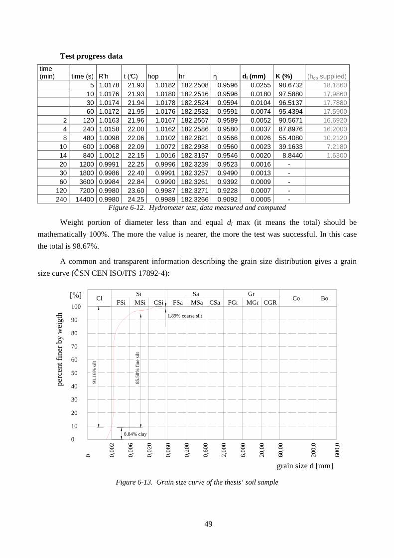
Figure 6-12. Hydrometer test, data measured and computed

Weight portion of diameter less than and equal di max (it means the total) should be

mathematically 100%. The more the value is nearer, the more the test was successful. In this case

the total is 98.67%.

A common and transparent information describing the grain size distribution gives a grain

size curve (ČSN CEN ISO/ITS 17892-4):

0

10

20

30

40

50

60

70

80

90

100

0,00

2

0,06

0

2,00

0

60,0

0

200,

0

600,

0

grain size d [mm]

pe

rce

nt fi

ner

by

wei

gth

[%] ClSi Sa Gr

Co BoFSi MSi CSi CSaMSaFSa CGRMGrFGr

0,20

0

0,60

0

6,00

0

20,0

0

0,02

0

0,00

6

0

85.

58%

fin

e si

lt

8.84% clay

1.89% coarse silt

91.

16%

silt

Figure 6-13. Grain size curve of the thesis‘ soil sample

50

6.5. Specimen Classification

Enough tests for the specimen classifying were performed. It is now possible to determine, to

which kind of soil the specimen belongs. The soil classification is discussed in chapter 3 in detail.

Thus the specimen employed in this thesis belongs according to the plasticity chart (Figure

3-4), according to the triangular diagram (used in the Czech Republic, Figure 3-5) to the group SH:

„Elastic inorganic silt with moderate to high plasticity“ (USCS, Figure 3-2), or to the group clSi

(Figure 3-5).

6.6. Pure Compression

Specimen characterisation

The specimen is cylinder-shaped. Moisture was added – the aim was to moisten the

specimen to get the optimal moisture content (29.41%) assessed by the Proctor test, chapter 4.4.

d (diameter, mm) 40 h (height, mm) 80 w (wetness, %) 30.2

Determination of normal stress

The values were computed according to the elementary physical relationship:

A

F=σ where F…force affecting the specimen, (9)

A…area subjected to the force,

which is in case of a cylinder defined

A = π r2 (10)

Taken from these relationships and the calibration curve for the measuring ring (Figure

6-15), the definite equation for determining the main (normal, vertical) stress has this image:

)(10

4

0237.0003.0 62

kPad

GR ⋅+⋅=π

σ (11)

where GR…Gauge Reading from the triaxial load ring.

51

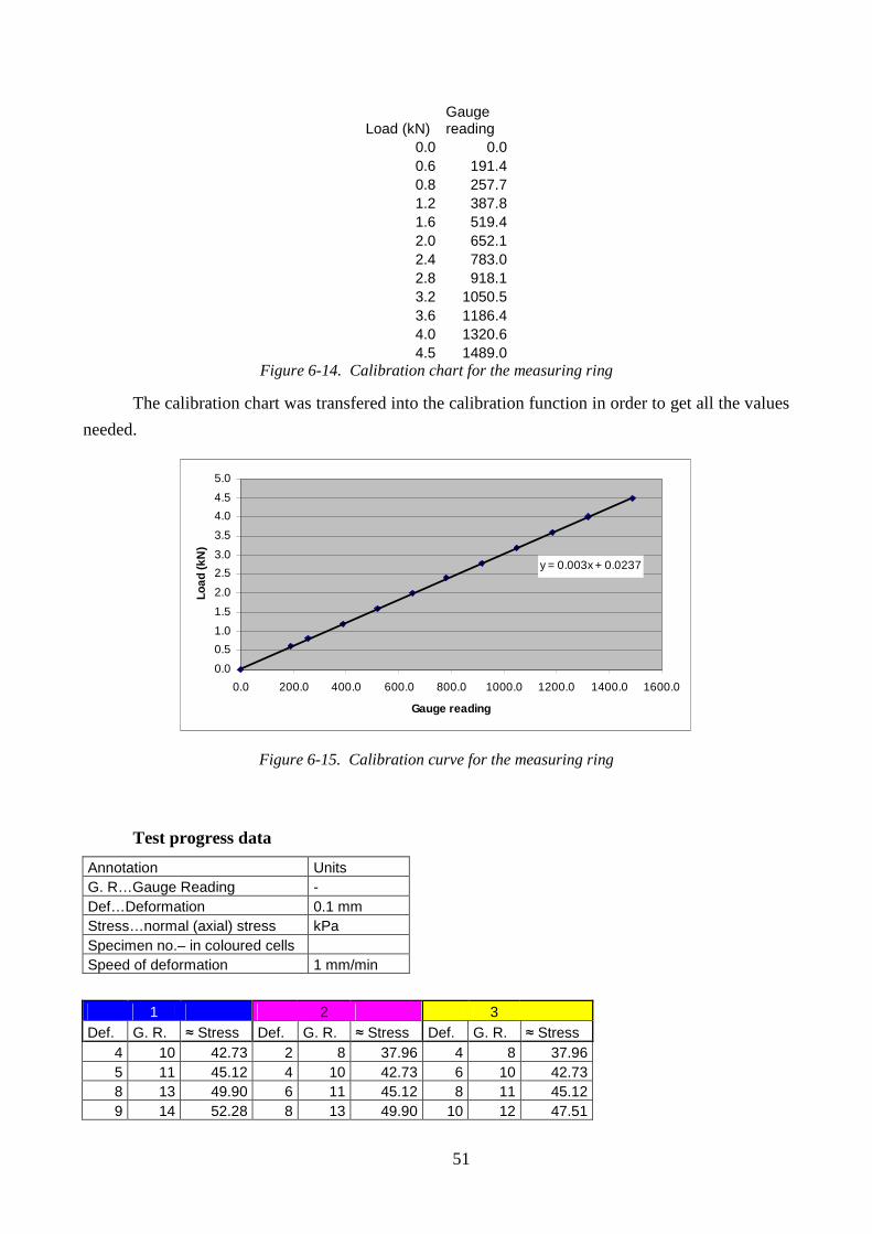
Load (kN) Gauge reading

0.0 0.0 0.6 191.4 0.8 257.7 1.2 387.8 1.6 519.4 2.0 652.1 2.4 783.0 2.8 918.1 3.2 1050.5 3.6 1186.4 4.0 1320.6 4.5 1489.0

Figure 6-14. Calibration chart for the measuring ring

The calibration chart was transfered into the calibration function in order to get all the values

needed.

y = 0.003x + 0.0237

0.0

0.5

1.0

1.5

2.0

2.5

3.0

3.5

4.0

4.5

5.0

0.0 200.0 400.0 600.0 800.0 1000.0 1200.0 1400.0 1600.0

Gauge reading

Load

(kN

)

Figure 6-15. Calibration curve for the measuring ring

Test progress data

Annotation Units G. R…Gauge Reading - Def…Deformation 0.1 mm Stress…normal (axial) stress kPa Specimen no.– in coloured cells Speed of deformation 1 mm/min

1 2 3 Def. G. R. ≈ Stress Def. G. R. ≈ Stress Def. G. R. ≈ Stress

4 10 42.73 2 8 37.96 4 8 37.96 5 11 45.12 4 10 42.73 6 10 42.73 8 13 49.90 6 11 45.12 8 11 45.12 9 14 52.28 8 13 49.90 10 12 47.51

52

1 2 3 Def. G. R. ≈ Stress Def. G. R. ≈ Stress Def. G. R. ≈ Stress

10 15 54.67 10 14 52.28 14 14 52.28 11 16 57.06 12 15 54.67 16 15 54.67 13 17 59.44 14 16 57.06 19 16 57.06 15 19 64.22 16 17 59.44 21 17 59.44 17 20 66.61 17 18 61.83 23 18 61.83 18 21 68.99 20 19 64.22 26 19 64.22 20 22 71.38 22 20 66.61 28 20 66.61 22 23 73.77 25 21 68.99 31 21 68.99 24 24 76.16 28 22 71.38 34 22 71.38 25 25 78.54 30 23 73.77 38 23 73.77 28 26 80.93 33 24 76.16 41 24 76.16 29 27 83.32 36 25 78.54 44 25 78.54 33 29 88.09 40 26 80.93 48 26 80.93 35 30 90.48 42 27 83.32 52 27 83.32 38 31 92.87 45 28 85.70 57 28 85.70 41 32 95.25 49 29 88.09 62 29 88.09 44 33 97.64 52 30 90.48 69 30 90.48 47 34 100.03 56 31 92.87 90 31 92.87 50 35 102.42 59 32 95.25 100 30 90.48 53 36 104.80 64 33 97.64 56 37 107.19 68 34 100.03 60 38 109.58 72 35 102.42 65 39 111.97 78 36 104.80 73 40 114.35 83 37 107.19 90 41 116.74 92 38 109.58

100 39 111.97 100 39 111.97 115 39 111.97 120 38 109.58

Figure 6-16. Pure compression test, data measured and computed

The specimens average stress bearing capacity is given by the arithmetic mean of the highest

Stress values, which is 107 kPa.

Acquired data were plotted in the stress-deformation graph for single specimens:

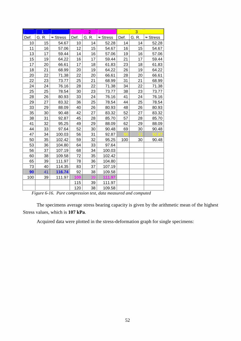
53

0.00

20.00

40.00

60.00

80.00

100.00

120.00

140.00

0 50 100 150

Shortening of specimen (deformation) (0.1 mm)

Str

ess

(kP

a) Specimen 1

Specimen 2

Specimen 3

Figure 6-17. Pure compression test, stress-deformation curves

As obvious from the graph, the duration of the specimen behaviour under graduating stress is

a smooth, nonlinear, gradually less growing function, until the point of the bearing capacity, where

the function growth stops and usually starts to fall rapidly.

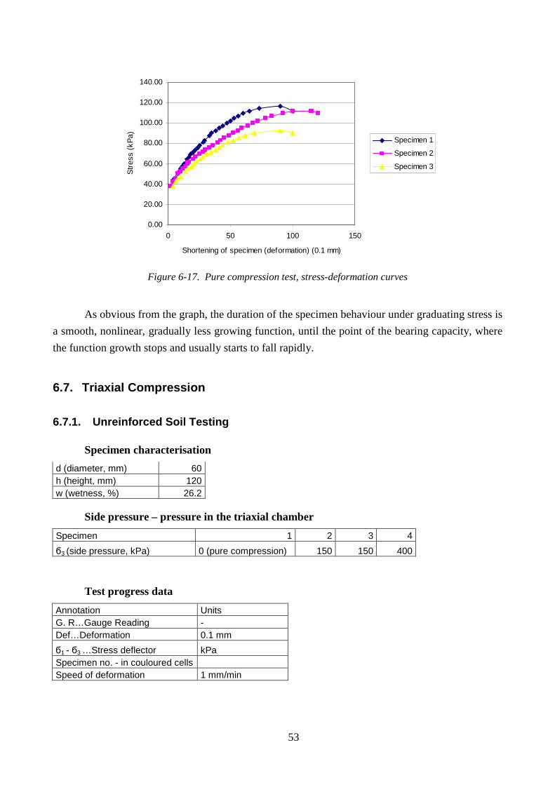
6.7. Triaxial Compression

6.7.1. Unreinforced Soil Testing

Specimen characterisation

d (diameter, mm) 60 h (height, mm) 120 w (wetness, %) 26.2

Side pressure – pressure in the triaxial chamber

Specimen 1 2 3 4

б3 (side pressure, kPa) 0 (pure compression) 150 150 400

Test progress data

Annotation Units G. R…Gauge Reading - Def…Deformation 0.1 mm

б1 - б3 …Stress deflector kPa Specimen no. - in couloured cells Speed of deformation 1 mm/min

54

1 2 3 4

Def. G. R. б1 - б3 Def. G. R. б1 - б3 Def. G. R. б1 - б3 Def. G. R. б1 - б3 2 10 18.99 2 20 29.60 10 20 29.60 3.5 30 40.21

5.5 20 29.60 4.3 40 50.82 13 40 50.82 6 50 61.43 7.5 30 40.21 9 60 72.04 18 60 72.04 11 70 82.65 12 40 50.82 15 80 93.26 25 80 93.26 14.5 80 93.26

15 45 56.13 23 100 114.49 37 100 114.49 24 100 114.49 17 50 61.43 25.5 105 119.79 51 115 130.40 30 110 125.10 19 55 66.74 31 115 130.40 60 120 135.71 38.5 120 135.71 22 60 72.04 34 120 135.71 75 130 146.32 49 130 146.32 25 65 77.35 38 125 141.01 91 135 151.62 61.5 140 156.93

28.5 70 82.65 42.5 130 146.32 111 138 154.80 81 150 167.54 32 75 87.96 48 135 151.62 139 137 153.74 101 155 172.84

34.5 78 91.14 53 139 155.87 150 136 152.68 106 156 173.90 36 80 93.26 54.5 140 156.93 115 157 174.96 38 82 95.39 59 143 160.11 130 158 176.03 40 85 98.57 63 145 162.23 145 157 174.96 44 88 101.75 72 148 165.42 152 156 173.90 46 90 103.88 76.5 149 166.48 48 92 106.00 80 150 167.54 52 95 109.18 84 151 168.60

59.5 100 114.49 90 152 169.66 64 102 116.61 95.5 153 170.72 70 105 119.79 105 154 171.78 77 107 121.91 112 155 172.84 84 109 124.03

100 108 122.97 101.5 107 121.91 103.5 105 119.79

Figure 6-18. Triaxial test of unreinforced soil, data measured and computed

Where б1 - б3 is a difference between the principal stresses – axial (normal) and side

(chamber – induced by water in the triaxial chamber).

The test with 150 kPa side pressure was conducted 2 times, thus the values are represented

by an average stress value, which is 163.82 kPa.

55

0.00

20.00

40.00

60.00

80.00

100.00

120.00

140.00

160.00

180.00

0 50 100 150 200

Shortening of specimen (deformation) (0.1 mm)

б1

- б

3 (

kPa

)

Specimen 1 (0 kPa)

Specimen 2 (150 kPa)

Specimen 3 (150 kPa)

Specimen 4 (400 kPa)

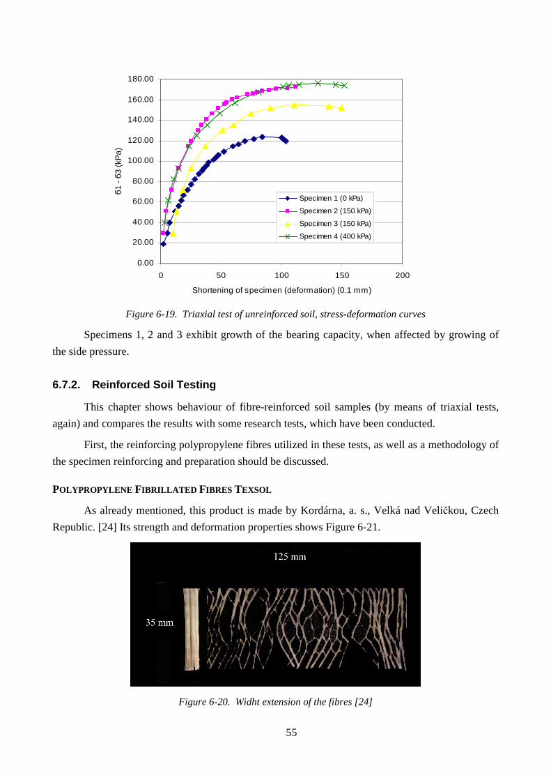
Figure 6-19. Triaxial test of unreinforced soil, stress-deformation curves

Specimens 1, 2 and 3 exhibit growth of the bearing capacity, when affected by growing of

the side pressure.

6.7.2. Reinforced Soil Testing

This chapter shows behaviour of fibre-reinforced soil samples (by means of triaxial tests,

again) and compares the results with some research tests, which have been conducted.

First, the reinforcing polypropylene fibres utilized in these tests, as well as a methodology of

the specimen reinforcing and preparation should be discussed.

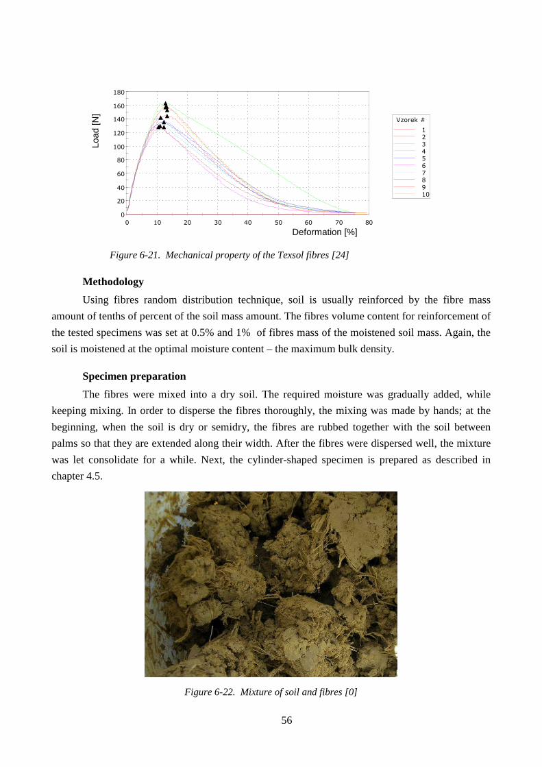
POLYPROPYLENE FIBRILLATED FIBRES TEXSOL

As already mentioned, this product is made by Kordárna, a. s., Velká nad Veličkou, Czech

Republic. [24] Its strength and deformation properties shows Figure 6-21.

Figure 6-20. Widht extension of the fibres [24]

56

Figure 6-21. Mechanical property of the Texsol fibres [24]

Methodology

Using fibres random distribution technique, soil is usually reinforced by the fibre mass

amount of tenths of percent of the soil mass amount. The fibres volume content for reinforcement of

the tested specimens was set at 0.5% and 1% of fibres mass of the moistened soil mass. Again, the

soil is moistened at the optimal moisture content – the maximum bulk density.

Specimen preparation

The fibres were mixed into a dry soil. The required moisture was gradually added, while

keeping mixing. In order to disperse the fibres thoroughly, the mixing was made by hands; at the

beginning, when the soil is dry or semidry, the fibres are rubbed together with the soil between

palms so that they are extended along their width. After the fibres were dispersed well, the mixture

was let consolidate for a while. Next, the cylinder-shaped specimen is prepared as described in

chapter 4.5.

Figure 6-22. Mixture of soil and fibres [0]

0

20

40

60

80

100

120

140

160

180

0 10 20 30 40 50 60 70 80

Skutečné přetvoření (%)

Vzorek #

12345678910

Load

[N]

Deformation [%]

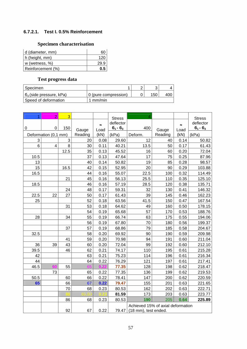
57

6.7.2.1. Test I. 0.5% Reinforcement

Specimen characterisation

d (diameter, mm) 60 h (height, mm) 120 w (wetness, %) 29.9 Reinforcement (%) 0.5

Test progress data

Specimen 1 2 3 4

б3 (side pressure, kPa) 0 (pure compression) 0 150 400 Speed of deformation 1 mm/min

1 2 3 4

0 0 150

Stress deflector б1 - б3 400

Stress deflector б1 - б3

Deformation (0,1 mm) Gauge

Reading

≈ Load (kN) (kPa) Deform.

Gauge Reading

≈ Load (kN) (kPa)

3 3 20 0.08 29.60 12 40 0.14 50.82 6 4 8 30 0.11 40.21 13.5 50 0.17 61.43

12.5 35 0.13 45.52 16 60 0.20 72.04 10.5 37 0.13 47.64 17 75 0.25 87.96

13 40 0.14 50.82 19 85 0.28 98.57 15 16.5 42 0.15 52.95 20 90 0.29 103.88

16.5 44 0.16 55.07 22.5 100 0.32 114.49 21 45 0.16 56.13 25.5 110 0.35 125.10

18.5 46 0.16 57.19 28.5 120 0.38 135.71 24 48 0.17 59.31 32 130 0.41 146.32

22.5 22 27 50 0.17 61.43 39 145 0.46 162.23 25 52 0.18 63.56 41.5 150 0.47 167.54

31 53 0.18 64.62 49 160 0.50 178.15 54 0.19 65.68 57 170 0.53 188.76

28 34 55 0.19 66.74 63 175 0.55 194.06 56 0.19 67.80 70 180 0.56 199.37 37 57 0.19 68.86 79 185 0.58 204.67

32.5 58 0.20 69.92 90 190 0.59 209.98 41 59 0.20 70.98 94 191 0.60 211.04

36 39 43 60 0.20 72.04 99 192 0.60 212.10 39.5 46 62 0.21 74.17 110 195 0.61 215.28

42 63 0.21 75.23 114 196 0.61 216.34 44 64 0.22 76.29 121 197 0.61 217.41

46.5 60 55 65 0.22 77.35 128 198 0.62 218.47 73 65 0.22 77.35 136 199 0.62 219.53

50.5 60 66 0.22 78.41 147 200 0.62 220.59 65 66 67 0.22 79.47 155 201 0.63 221.65

70 68 0.23 80.53 162 202 0.63 222.71 80 69.00 0.23 81.59 173 203 0.63 223.77 86 68 0.23 80.53 190 205 0.64 225.89

92 67 0.22 79.47 Achieved 15% of axial deformation (18 mm), test ended.

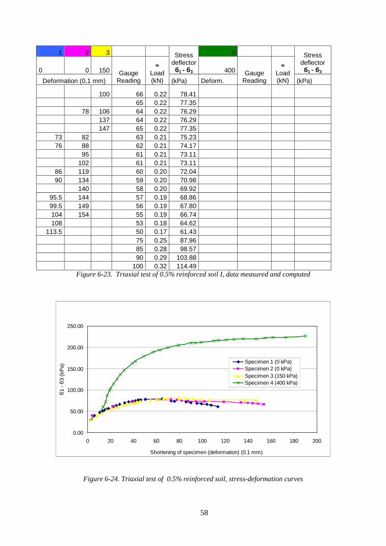
58

1 2 3 4

0 0 150

Stress deflector б1 - б3 400

Stress deflector б1 - б3

Deformation (0,1 mm) Gauge

Reading

≈ Load (kN) (kPa) Deform.

Gauge Reading

≈ Load (kN) (kPa)

100 66 0.22 78.41

65 0.22 77.35 78 106 64 0.22 76.29 137 64 0.22 76.29 147 65 0.22 77.35

73 82 63 0.21 75.23 76 88 62 0.21 74.17

95 61 0.21 73.11 102 61 0.21 73.11

86 119 60 0.20 72.04 90 134 59 0.20 70.98

140 58 0.20 69.92 95.5 144 57 0.19 68.86 99.5 149 56 0.19 67.80 104 154 55 0.19 66.74 108 53 0.18 64.62

113.5 50 0.17 61.43 75 0.25 87.96 85 0.28 98.57 90 0.29 103.88 100 0.32 114.49

Figure 6-23. Triaxial test of 0.5% reinforced soil I, data measured and computed

Figure 6-24. Triaxial test of 0.5% reinforced soil, stress-deformation curves

0.00

50.00

100.00

150.00

200.00

250.00

0 20 40 60 80 100 120 140 160 180 200

Shortening of specimen (deformation) (0.1 mm)

б1

- б

3 (k

Pa)

Specimen 1 (0 kPa)Specimen 2 (0 kPa)Specimen 3 (150 kPa)Specimen 4 (400 kPa)

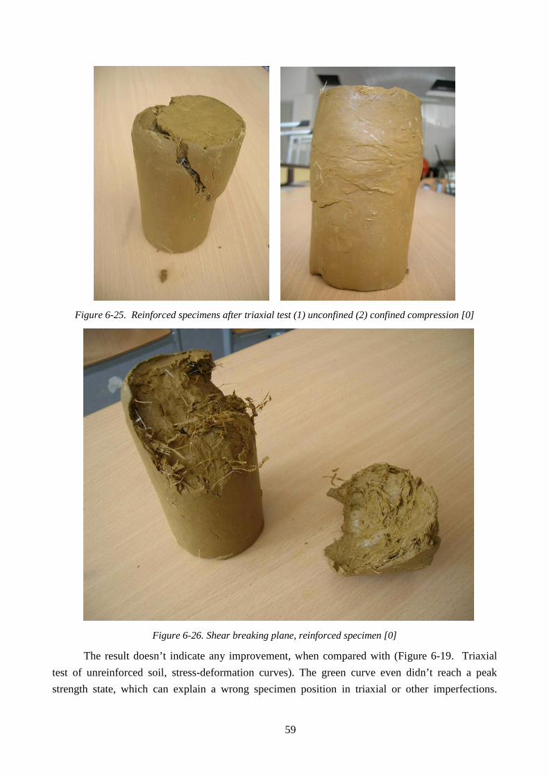
59

Figure 6-25. Reinforced specimens after triaxial test (1) unconfined (2) confined compression [0]

Figure 6-26. Shear breaking plane, reinforced specimen [0]

The result doesn’t indicate any improvement, when compared with (Figure 6-19. Triaxial

test of unreinforced soil, stress-deformation curves). The green curve even didn’t reach a peak

strength state, which can explain a wrong specimen position in triaxial or other imperfections.

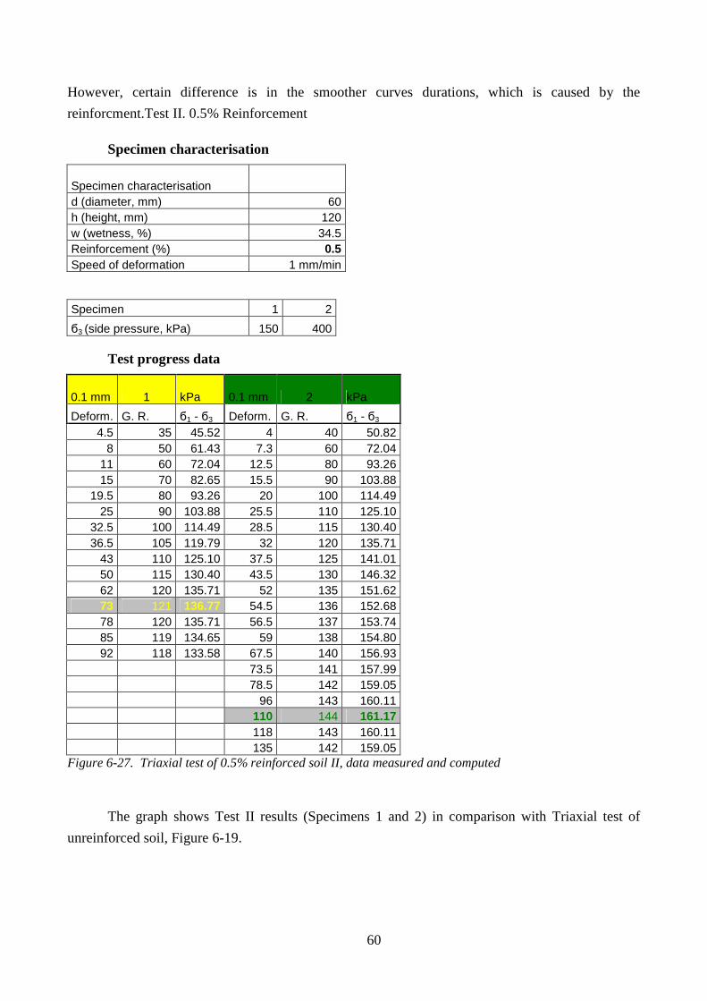
60

However, certain difference is in the smoother curves durations, which is caused by the

reinforcment.Test II. 0.5% Reinforcement

Specimen characterisation

Specimen characterisation d (diameter, mm) 60 h (height, mm) 120 w (wetness, %) 34.5 Reinforcement (%) 0.5 Speed of deformation 1 mm/min

Specimen 1 2

б3 (side pressure, kPa) 150 400

Test progress data

0.1 mm 1 kPa 0.1 mm 2 kPa

Deform. G. R. б1 - б3 Deform. G. R. б1 - б3 4.5 35 45.52 4 40 50.82

8 50 61.43 7.3 60 72.04 11 60 72.04 12.5 80 93.26 15 70 82.65 15.5 90 103.88

19.5 80 93.26 20 100 114.49 25 90 103.88 25.5 110 125.10

32.5 100 114.49 28.5 115 130.40 36.5 105 119.79 32 120 135.71

43 110 125.10 37.5 125 141.01 50 115 130.40 43.5 130 146.32 62 120 135.71 52 135 151.62 73 121 136.77 54.5 136 152.68 78 120 135.71 56.5 137 153.74 85 119 134.65 59 138 154.80 92 118 133.58 67.5 140 156.93

73.5 141 157.99 78.5 142 159.05 96 143 160.11 110 144 161.17 118 143 160.11 135 142 159.05 Figure 6-27. Triaxial test of 0.5% reinforced soil II, data measured and computed

The graph shows Test II results (Specimens 1 and 2) in comparison with Triaxial test of

unreinforced soil, Figure 6-19.

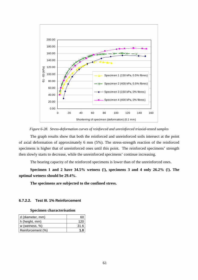
61

0.00

20.00

40.00

60.00

80.00

100.00

120.00

140.00

160.00

180.00

200.00

0 20 40 60 80 100 120 140 160

Shortening of specimen (deformation) (0.1 mm)

б1

- б

3 (

kPa

)

Specimen 1 (150 kPa, 0.5% fibres)

Specimen 2 (400 kPa, 0.5% fibres)

Specimen 3 (150 kPa, 0% fibres)

Specimen 4 (400 kPa, 0% fibres)

Figure 6-28. Stress-deformation curves of reinforced and unreinforced triaxial-tested samples

The graph results show that both the reinforced and unreinforced soils intersect at the point

of axial deformation of approximately 6 mm (5%). The stress-strength reaction of the reinforced

specimens is higher that of unreinforced ones until this point. The reinforced specimens’ strength

then slowly starts to decrease, while the unreinforced specimens‘ continue increasing.

The bearing capacity of the reinforced specimens is lower than of the unreinforced ones.

Specimen 1 and 2 have 34.5% wetness (!), specimens 3 and 4 only 26.2% (!). The

optimal wetness should be 29.4%.

The specimens are subjected to the confined stress.

6.7.2.2. Test III. 1% Reinforcement

Specimen characterisation

d (diameter, mm) 60 h (height, mm) 120 w (wetness, %) 31.6 Reinforcement (%) 1.0

62

Test progress data

Deformation speed (mm/min) 1

Specimen 1 2 3 б3 (side pressure, kPa) 0 150 400

1 2 3

Jaw shift (0,1 mm) Gauge Reading

≈ Load (kN)

б1 - б3

(kPa) Jaw shift

Gauge Reading

≈ Load (kN) б1 - б3

3.5 20 0.08 29.60 11 90 0.29 103.88 7 4 30 0.11 40.21 14 100 0.32 114.49

11 40 0.14 50.82 17 110 0.35 125.10 13.5 45 0.16 56.13 22.5 125 0.40 141.01 16.5 7.5 50 0.17 61.43 25 130 0.41 146.32

20 55 0.19 66.74 29.5 140 0.44 156.93 23.5 60 0.20 72.04 36.5 150 0.47 167.54

28 65 0.22 77.35 45 160 0.50 178.15 32 12.5 70 0.23 82.65 50 165 0.52 183.45

37.5 75 0.25 87.96 56 170 0.53 188.76 41.5 78 0.26 91.14 64.5 175 0.55 194.06

45 15 80 0.26 93.26 74 180 0.56 199.37 49 82 0.27 95.39 79 182 0.57 201.49

51.5 83 0.27 96.45 81 183 0.57 202.55 53.5 84 0.28 97.51 88 184 0.58 203.61

55 85 0.28 98.57 94 185 0.58 204.67 57.5 86 0.28 99.63 97 186 0.58 205.73

61 87 0.28 100.69 104 187 0.58 206.80 64.5 88 0.29 101.75 131 188 0.59 207.86

72 89 0.29 102.81 165 186 0.58 205.73 81 19 90 0.29 103.88 95 91 0.30 104.94

116 90 0.29 103.88 136 89 0.29 102.81 144 88 0.29 101.75 155 87 0.28 100.69

22.5 100 0.32 114.49 28 110 0.35 125.10 34 120 0.38 135.71 39 125 0.40 141.01 44 130 0.41 146.32 50 135 0.43 151.62 56.5 140 0.44 156.93 62 143 0.45 160.11 77 150 0.47 167.54 80 151 0.48 168.60 82 152 0.48 169.66

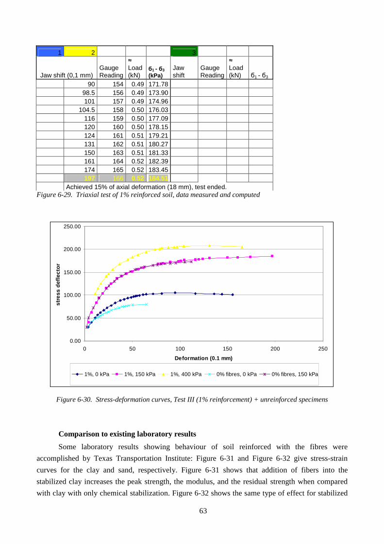
63

1 2 3

Jaw shift (0,1 mm) Gauge Reading

≈ Load (kN)

б1 - б3

(kPa) Jaw shift

Gauge Reading

≈ Load (kN) б1 - б3

90 154 0.49 171.78 98.5 156 0.49 173.90 101 157 0.49 174.96 104.5 158 0.50 176.03 116 159 0.50 177.09 120 160 0.50 178.15 124 161 0.51 179.21 131 162 0.51 180.27 150 163 0.51 181.33 161 164 0.52 182.39 174 165 0.52 183.45 197 166 0.52 184.51 Achieved 15% of axial deformation (18 mm), test ended. Figure 6-29. Triaxial test of 1% reinforced soil, data measured and computed

0.00

50.00

100.00

150.00

200.00

250.00

0 50 100 150 200 250

Deformation (0.1 mm)

stre

ss d

efle

ctor

1%, 0 kPa 1%, 150 kPa 1%, 400 kPa 0% fibres, 0 kPa 0% fibres, 150 kPa

Figure 6-30. Stress-deformation curves, Test III (1% reinforcement) + unreinforced specimens

Comparison to existing laboratory results

Some laboratory results showing behaviour of soil reinforced with the fibres were

accomplished by Texas Transportation Institute: Figure 6-31 and Figure 6-32 give stress-strain

curves for the clay and sand, respectively. Figure 6-31 shows that addition of fibers into the

stabilized clay increases the peak strength, the modulus, and the residual strength when compared

with clay with only chemical stabilization. Figure 6-32 shows the same type of effect for stabilized

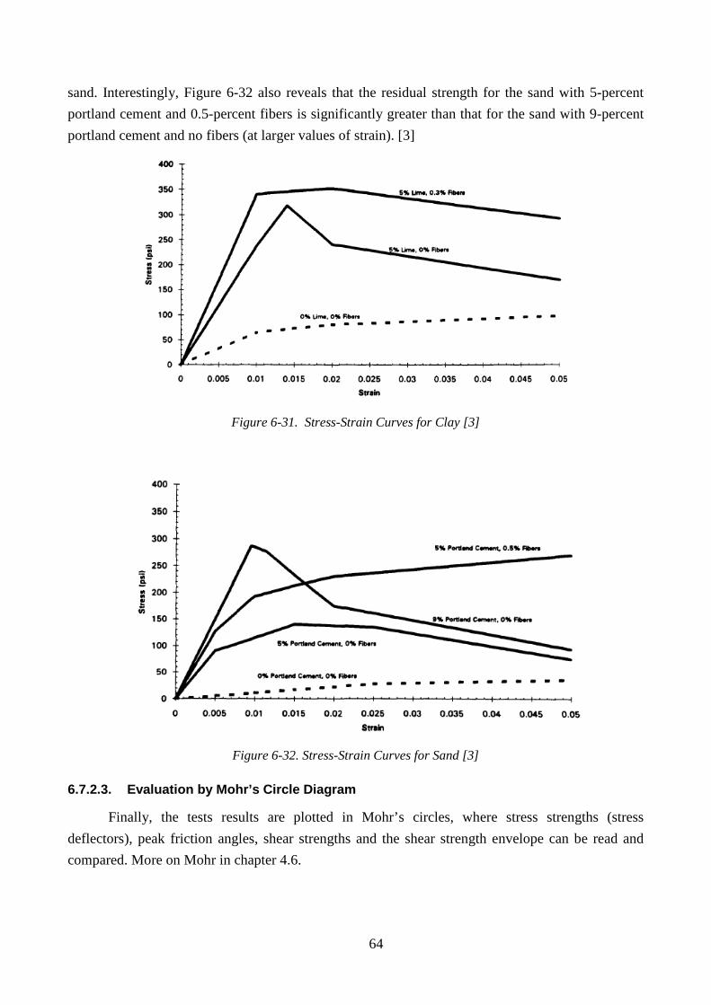
64

sand. Interestingly, Figure 6-32 also reveals that the residual strength for the sand with 5-percent

portland cement and 0.5-percent fibers is significantly greater than that for the sand with 9-percent

portland cement and no fibers (at larger values of strain). [3]

Figure 6-31. Stress-Strain Curves for Clay [3]

Figure 6-32. Stress-Strain Curves for Sand [3]

6.7.2.3. Evaluation by Mohr’s Circle Diagram

Finally, the tests results are plotted in Mohr’s circles, where stress strengths (stress

deflectors), peak friction angles, shear strengths and the shear strength envelope can be read and

compared. More on Mohr in chapter 4.6.

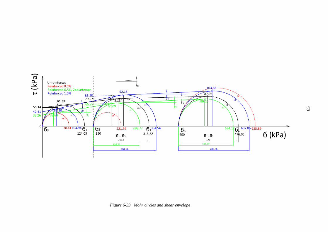
65

Figure 6-33. Mohr circles and shear envelope

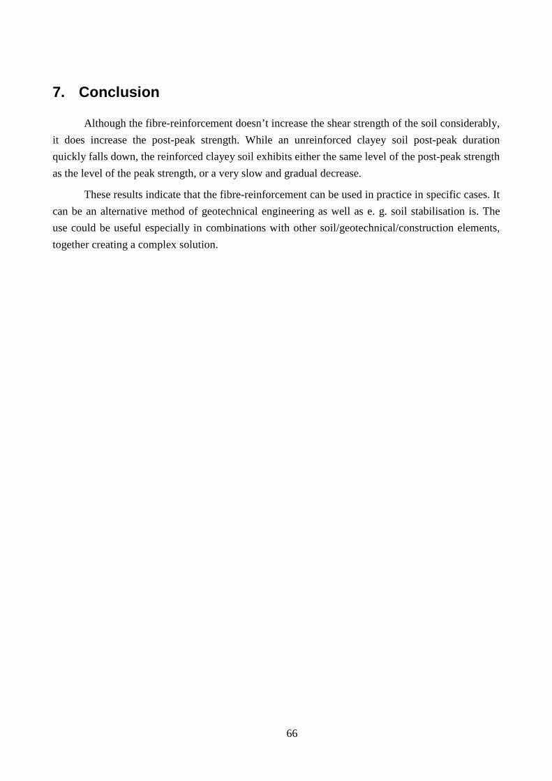
66

7. Conclusion

Although the fibre-reinforcement doesn’t increase the shear strength of the soil considerably,

it does increase the post-peak strength. While an unreinforced clayey soil post-peak duration

quickly falls down, the reinforced clayey soil exhibits either the same level of the post-peak strength

as the level of the peak strength, or a very slow and gradual decrease.

These results indicate that the fibre-reinforcement can be used in practice in specific cases. It

can be an alternative method of geotechnical engineering as well as e. g. soil stabilisation is. The

use could be useful especially in combinations with other soil/geotechnical/construction elements,

together creating a complex solution.

67

BIBLIOGRAPHY

[0] Author’s pictures taken in the faculty geotechnical laboratory, yr 2009.

[1] Holtz, D. Robert. Geosynthetics for Soil Reinforcement [online]. Seattle, Washington,

November 2001.

URL:

https://ceprofs.civil.tamu.edu/briaud/Buchanan%20Web/Lectures/Ninth%20Buchanan%20Lecture.

pdf [cit. 2009-03-18].

[2] Zornberg, Jorge G. Advances in Reinforced Soil Technology [online]. Department of Civil,

Architectural and Environmental Engineering, University of Texas at Austin, 2005.

URL: http://www.ce.utexas.edu/prof/zornberg/zornberg-

publication_files/Zornberg/Zornberg%20nonreferreed/Zornberg_2005.pdf [cit. 2009-03-18].

[3] Grogan, William P.; Johnson, Wayne G. Stabilization of High Plasticity Clay and Silty Sand by

Inclusion of Discrete Fibrillated Polypropylene Fibers (Fibergrids®) for Use in Pavement

Subgrades. U.S. Army Corps of Engineers, May 1994. Final Report CPAR-GL-94-2.

[4] Li, Chunling. Mechanical Response of Fiber-reinforced Soil [online]. Dissertation Thessis, The

University of Texas at Austin, May 2005.

URL: https://repositories.lib.utexas.edu/bitstream/handle/2152/1781/lic25697.pdf?sequence=2.

[cit. 2009-03-18].

[5] Integrated Publishing [online].

URL: http://www.tpub.com/content/engineering/14071/css/14071_389.htm [cit. 2009-05-15].

[6] Day, Robert W. Soil testing manual: procedures, classification data, and sampling practices.

McGraw-Hill Professional, 2001. ISBN 0071363637, 9780071363631.

[7] Cvičení č. 3: Stanovení zrnitosti zemin. Department of Infrastructure: Geotechnika a zakládání

staveb, Jan Perner Transport Faculty.

[8] Atterberg limits [online]. Wikipedia, the free encyclopedia, last modification 2009-05-19.

URL: http://en.wikipedia.org/wiki/Atterberg_limits [cit. 2009-05-17].

[9] Liquid Limit: Cone Penetrometer Method [online]. Main Roads Western Australia. Issue 1

09/87.

URL: http://www2.mainroads.wa.gov.au/NR/rdonlyres/688EAC66-D077-4500-A017-

6885F869B196/0/wa120_2.pdf [cit. 2009-05-17].

[10] Plasticity Chart for the Unified Soil Classification System [online]. Last modified 2006-12-19.

URL: http://www.crma.ac.th/cedept/CourseWare/Geotech/CE4304/Chapter1/Images/PlastChart.gif

[cit. 2009-05-18].

[11] Unified Soil Classification System – ASTM D2488 [online]. Gint Software, last revision

2005-09-26.

URL: http://www.gintsoftware.com/downloads/reports/lgd_a_nnnn03.pdf [cit. 2009-05-18].

[12] Grain Size Distribution [online]. University of Texas at Arlington, Thursday 02-05-04.

68

URL: http://geotech.uta.edu/lab/Main/Soil%20Lab/03_Sieve%20analysis/Sieve%20analysis.pdf

[cit. 2009-05-20].

[13] Geotextile [online]. Germes Online.

URL: http://www.germes-online.com/catalog/13/701/128620/geotextile.html [cit. 2009-05-20].

[14] Geogrids: http://www.permathene.com/htm/photographs/photo_geogrids.shtml [cit. 2009-03-

18].

[15] Geonet: http://www.germes-online.com/direct/dbimage/50086415/Geonet.jpg [cit. 2009-03-

18].

[16] Geotechnical Laboratory Experiments [online].

URL: http://home.iitk.ac.in/~madhav/geolab.html [cit. 2009-05-20].

[17] ENCE 361 Soil Mechanics: Unconfined Compression Test [online]. Vulcanhammer.net.

URL: http://www.vulcanhammer.net/utc/ence361/f2001/361-ll8.pdf [cit. 2009-05-20].

[18] Stress-strain curve [online]. Wikipedia, the free encyclopedia, last modified on 18 May 2009.

URL: http://en.wikipedia.org/wiki/Stress-strain_curve [cit. 2009-05-21].

[19] Lamboj, L.; Štěpánek, Z. Mechanika zemin a zakládání staveb. ČVUT, 2005.

[20] Operating Instruction: Multiplex 50. ELE International, 2004. 9901X0236 Issue 3.

[21] http://www.kern-vahy.cz/cz/partnershop/catalogue-28.html [cit. 2009-05-22].

[22] Newark.

URL: http://www.newark.com/jsp/search/productdetail.jsp?sku=53M7381&_requestid=275793.

[cit 2009-05-25].

[23] BMT. Venticell 111 [online].

URL:

http://www.bmt.cz/goodsdetail_ls.asp?nGoodsID=1355&nDepartmentID=284&nLanguageID=2

[cit. 2009-05-25].

[24] Šmejda, A. Experimentální posouzení stability vyztužených zemních těles. Dissertation work,

Jan Perner Transport Faculty, University of Pardubice, August 2008.

[25] Cvičení č. 4: Pojmenování, popis a zatřídění zemin. Department of Infrastructure: Geotechnika

a zakládání staveb, Jan Perner Transport Faculty.