University of Mannheim / Department of Economics

Working Paper Series

Do Girls Really Outperform Boys in Educational Outcomes?

Perihan Ozge Saygin

Working Paper 14-05

February 2014

Do Girls Really Outperform Boys in EducationalOutcomes?∗

Perihan Ozge SayginUniversity of Mannheim

February 25, 2014

Abstract

The reversing achievement gap across genders observed in many countries hasled to a heated debate on the persistent gap in academia and other top fields. UsingTurkish administrative data and the particular institutional characteristics, this pa-per aims to analyze the gender gap in educational outcomes from different methodsof evaluation and the gender gap in college applications. The results contributeto the discussion of the gender gap in performance in education suggesting thatevaluation systems might have gender biased impacts on students and the under-representation of females in top fields can not be explained by differences in testscores.

JEL Classification: C35, I20, I24Keywords: gender gap, test scores, university entrance exam

∗I am indebted to David Card and Francesca Lotti for their advice and encouragement. I am grateful to the Student

Selection and Placement Center (OSYM in Turkish) in Turkey for sharing data. I would like to thank also Andrea Weber

for her insightful comments. All errors are mine. Email saygin@uni-mannheim.de

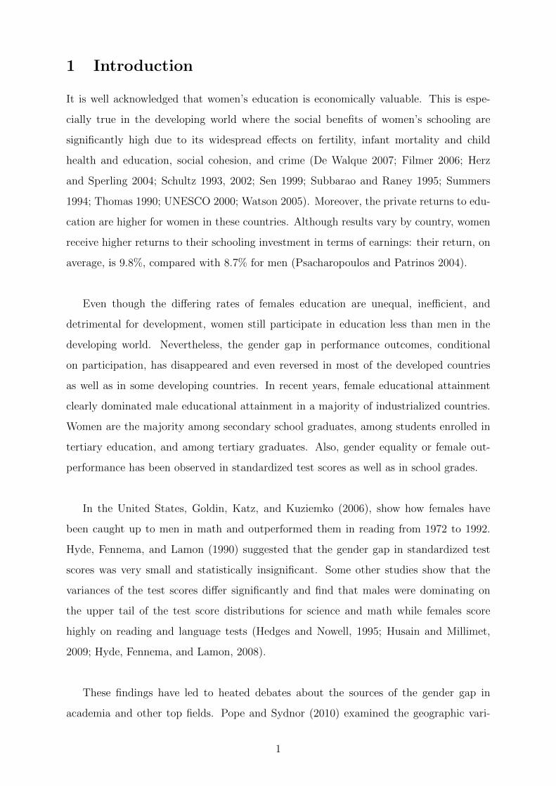
1 Introduction

It is well acknowledged that women’s education is economically valuable. This is espe-

cially true in the developing world where the social benefits of women’s schooling are

significantly high due to its widespread effects on fertility, infant mortality and child

health and education, social cohesion, and crime (De Walque 2007; Filmer 2006; Herz

and Sperling 2004; Schultz 1993, 2002; Sen 1999; Subbarao and Raney 1995; Summers

1994; Thomas 1990; UNESCO 2000; Watson 2005). Moreover, the private returns to edu-

cation are higher for women in these countries. Although results vary by country, women

receive higher returns to their schooling investment in terms of earnings: their return, on

average, is 9.8%, compared with 8.7% for men (Psacharopoulos and Patrinos 2004).

Even though the differing rates of females education are unequal, inefficient, and

detrimental for development, women still participate in education less than men in the

developing world. Nevertheless, the gender gap in performance outcomes, conditional

on participation, has disappeared and even reversed in most of the developed countries

as well as in some developing countries. In recent years, female educational attainment

clearly dominated male educational attainment in a majority of industrialized countries.

Women are the majority among secondary school graduates, among students enrolled in

tertiary education, and among tertiary graduates. Also, gender equality or female out-

performance has been observed in standardized test scores as well as in school grades.

In the United States, Goldin, Katz, and Kuziemko (2006), show how females have

been caught up to men in math and outperformed them in reading from 1972 to 1992.

Hyde, Fennema, and Lamon (1990) suggested that the gender gap in standardized test

scores was very small and statistically insignificant. Some other studies show that the

variances of the test scores differ significantly and find that males were dominating on

the upper tail of the test score distributions for science and math while females score

highly on reading and language tests (Hedges and Nowell, 1995; Husain and Millimet,

2009; Hyde, Fennema, and Lamon, 2008).

These findings have led to heated debates about the sources of the gender gap in

academia and other top fields. Pope and Sydnor (2010) examined the geographic vari-

1

ation in test scores and found significant variation across states and census divisions

suggesting that the gender gap is driven by differing social forces in different states rather

than gender differences in innate abilities.

A debate on evaluation techniques which also concerns the gender gap has critiqued the

use of standardized tests to select and/or assign students to schools or colleges (Connor

and Vargyas, 1992; Medina et al. 1990; Rosser, 1989). Moreover, a literature on gender

differences in social preferences and attitudes towards competition has developed in recent

years. This literature provides consistent evidence that females under-perform in com-

petitive environments. (Gneezy et. al., 2003; Paserman, 2007; Niederle and Vesterlund,

2007). These findings motivated other studies to explain gender differences in education

outcomes. Ors et al. (2013) show that the competitive nature of the evaluations explains

a significant part of the gender gap in academic examinations.

The aim of this paper is to provide an overview of the gender gap in educational at-

tainment in terms of the different evaluation methods used in Turkey-in particular in the

transition from high school to higher education. In particular, my contribution is two-fold.

First, I investigate whether the gender gap varies under different evaluation methods. To

answer this question, I compare the gender gap for the same students under different

evaluation measures where the combination of these outcomes determine the access to

university education. Second, after evaluating the gender gap in achievement, I analyze

the gender gap in assignment outcomes conditional on performance in high school and

standardized test in order to provide evidence for differences in preferences conditional

on outcomes.

Turkey is a very interesting case because the recent reports show interesting results

for the gender gap in educational outcomes in Turkey. According to PISA 2009 (OECD

2010), gender difference in reading performance is in favor of girls (43 points) and it is

above the OECD average which is 39 points. Girls also outperform boys in science by

17 points while the OECD average gender gap was equal to 0. The gender gap in math

performance is in favor of boys by 11 points but it is slightly lower than the OECD aver-

age which is 12 score points. Another interesting finding is that between PISA 2006 and

2

PISA 2009, performance in science improved only in 11 OECD countries and Turkey had

one of the best performance improvements in science. On the other hand, similar to most

developing countries, a sizable gap remains in overall schooling levels in Turkey.

In Turkey access to university education1 is only possible through a nation-wide univer-

sity entrance exam. The number of applicants exceeds far beyond the capacity of Turkish

universities; therefore college applicants compete fiercely for high-return major/degrees

in top universities. Applicants are evaluated according to their test scores as well as

high-school GPAs where high-school GPA has very small contribution to admission prob-

abilities. High-school GPA is calculated based on the weighted averages of the grades of

each written exam during the 4 years of high school education. The standardized test is

a multiple choice test of 3 hours conducted at a nat ional level only once a year. Final

assignment scores are calculated for each applicant as a weighted sum of standardized

test scores and high-school GPAs2 Finally, a centralized algorithm assigns applicants ac-

cording to their final assignment scores and their choices of university and major degrees

that applicants submit after receiving their results.

The biggest advantage of working on the gender gap in Turkey is that high school

GPAs and standardized multiple choice test scores are used together to evaluate students

for college admissions. The tracking system of secondary education and centralized sys-

tem of university applications based on a standardized test score and high-school GPAs

provide the opportunity to analyze the gender gap in high school grades, standardized test

scores as well as gender differences in likelihood of getting into a college. Moreover, this

specific institutional setting provides some insights for the usual problem of accounting

for the positive selection of females. I compare the results from a sample of retakers and

first-time takers to infer the direction of the potential selection bias assuming the sample

of retakers are much more exposed to the positive selection.

In this paper, I document the gender gap in educational outcomes using a sample of

1Both public and private universities accept students through the centralized system where the accessto private universites is less competitive.

2High-school GPA has a relatively small weight in the final score compared to the standardized testscore. High school GPAs are also corrected with certain coefficients according to the type of high school,average achievements of students in the school, and ranking of the applicant within the school.

3

Student Selection and Placement System (OSYS in Turkish) for the college admissions

in Turkey in 2008. After a descriptive analysis of data and a graphical analysis of gender

differences, I estimate the gender gap in the average as well as at different quantiles of

the test score and high-school GPA distributions. First, I explore the gender gap in high-

school GPAs in different high school tracks and I find very significant and large gender

gaps in favor of female students at all quantiles of high-school GPAs in all specialization

tracks. Second, I analyze the gender gap in standardized test scores in different subjects

and I find mixed results across subjects for different quantiles of the test score distribu-

tions. I then analyze the gender gap in assignment rates and find that after controlling

for test scores females are more likely to enroll in higher education programs in their

first attempt of university entrance test. Nevertheless, men still outnumber women at the

highly selective programs that lead to high-paying careers once we control for assignment

scores.

These findings are important not only because this is the first comprehensive study

on the gender gap in Turkey using administrative data but it also provides suggestive ev-

idence on the differing gender gap under different evaluation methods (high school grades

vs standardized test scores). Moreover it also underlines that the underrepresentation of

females in top fields can not be only explained in differences in test scores. My findings

shows that there is a clear gap in high school GPAs in favor of females at all quantiles of

the distribution in all subjects while the quantile regressions show that the gender gap in

standardized test scores remains in favor of males for both high and low ends of the test

score distributions. As it is stated earlier, high-school GPA and standardized test score

are combined to calculate a final assignment score to place students in line with their

preferences. In order to evaluate the overall gender gap in college application outcomes,

I also analyze the gender gap in final assignment scores where I find that females per-

form better on average while there is no significant difference in quantitative assignment

scores. Moreover, when we control for assignment scores and look at the differences in

major degrees it seems there are still significant gender differences in assignment rates to

top majors.

The findings of this paper are also consistent with the literature on gender differences

4

in social preferences such as attitude towards competition. The fact that female stu-

dents outperform males in terms of high school grades while they are not as successful

at standardized test raises the question that the effect of competitive environment and

application of 3 hours exam for a lifetime matter based on a multiple choice test might

have a negative effect on females especially on math and quantitative subjects. Findings

on the gender gap in assignment to a college degree also sheds some light on nature vs

nurture debate on cognitive ability and test scores which rose from the underrepresen-

tation of women in top fields explained by male domination in high test score intervals.

Obviously test score differences affect the gender gap in assignment rates but there is a

significant gap that remains unexplained by score differences alone which supports the

argument that there are differences in preferences for college choice.3

2 Education System in Turkey and An Overview of

the gender gap

The formal education system in Turkey consists of primary education, high school edu-

cation and university. The primary education is the only compulsory part and it consists

of 8 years. Until 1997, the primary education was only 5 years and the middle schools

that give 3 years education were not compulsory. In 1997, the compulsory education has

been extended to 8 years of basic education merging middle school with primary school

education.

After the compulsory education, the secondary level of schooling consists of high school

education which lasts 4 years or vocational high school education which prepares students

for entering the labor market.4 Allocation of primary school graduates to high schools

is also conducted by a centralized examination with a standardized test. Depending on

the test scores all students are sorted into different type of high schools in line with their

preferences. This examination is called the Secondary School Examination (OKS in Turk-

ish) and is administered by the Ministry of Education. The aim of this examination is

to restrict the access to special/top ranked high schools that are expected to provide a

3In a companion paper Saygin(2012) further evidence on gender differences in preferences in collegeand major choices is provided.

4Before 2006, there were also vocational and general type of high schools where the education durationwas 3 years. In 2006, all type of high schools started to give 4 years of education.

5

higher standard of education5. Those types include Anatolian High Schools, Scientific

High Schools, Foreign Language High Schools and some private high schools. There are

also general type high schools as well as vocational high schools that are open to every

student regardless of their test scores in the OKS. The OKS test scores therefore are only

important to students who aim to attend one of these special high schools.

After entering the high school, another important decision students face in their second

year of high school is the choice of a subject, namely sciences, social sciences, Turkish-

mathematics, foreign languages or arts. This specialization results in different curricula

focusing on the respecting subjects. General high schools offer a curriculum preparing

students for university education with a tracking system where students are expected to

be specialized in a subject and choose a future education or labor market career accord-

ingly. Similarly, the vocational high schools offer technical education preparing students

for vocational higher education within the higher education system. Some school types

allow specialization only in certain subjects, such as scientific high schools offer only sci-

ence as specialization subject.

Turkish government provides formal education for all the citizens free of charge at each

level. Primary and high school education is under the Ministry of Education’s control.

Together with public schools, there are also private schools at each stage of the education

system that is regulated again by the Ministry of Education. There are also privately

operated tutoring centers which both give additional support during the formal education

and also prepare students for both the OKS and university entrance examinations.

Access to university education is provided with a centralized system since 1974. Pri-

vate universities have started to operate in late 1980s. In 2008 there were around 160

universities in Turkey and around 35 of them were private universities. In the last couple

of years, the number of private universities have been sharply increasing and providing

college seats for many applicants. Both private and public universities provide 4-years

university programs as well as 2 years vocational programs. There is also the so-called

Open Education which is a distance learning system granting a four-year degree where

5Some of these schools provide the regular curriculum in a foreign language as instruction language

6

students follow lectures broadcast on national TV or online and sit for the centrally ad-

ministered examinations.

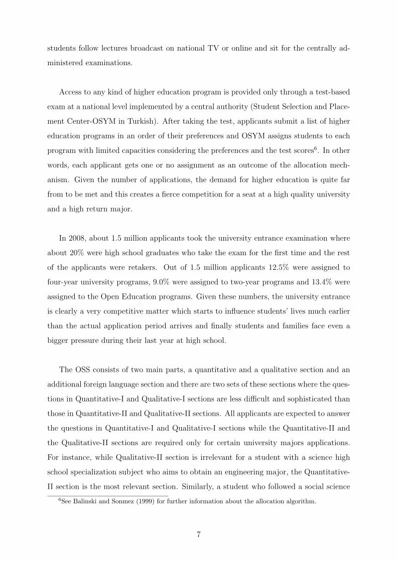
Access to any kind of higher education program is provided only through a test-based

exam at a national level implemented by a central authority (Student Selection and Place-

ment Center-OSYM in Turkish). After taking the test, applicants submit a list of higher

education programs in an order of their preferences and OSYM assigns students to each

program with limited capacities considering the preferences and the test scores6. In other

words, each applicant gets one or no assignment as an outcome of the allocation mech-

anism. Given the number of applications, the demand for higher education is quite far

from to be met and this creates a fierce competition for a seat at a high quality university

and a high return major.

In 2008, about 1.5 million applicants took the university entrance examination where

about 20% were high school graduates who take the exam for the first time and the rest

of the applicants were retakers. Out of 1.5 million applicants 12.5% were assigned to

four-year university programs, 9.0% were assigned to two-year programs and 13.4% were

assigned to the Open Education programs. Given these numbers, the university entrance

is clearly a very competitive matter which starts to influence students’ lives much earlier

than the actual application period arrives and finally students and families face even a

bigger pressure during their last year at high school.

The OSS consists of two main parts, a quantitative and a qualitative section and an

additional foreign language section and there are two sets of these sections where the ques-

tions in Quantitative-I and Qualitative-I sections are less difficult and sophisticated than

those in Quantitative-II and Qualitative-II sections. All applicants are expected to answer

the questions in Quantitative-I and Qualitative-I sections while the Quantitative-II and

the Qualitative-II sections are required only for certain university majors applications.

For instance, while Qualitative-II section is irrelevant for a student with a science high

school specialization subject who aims to obtain an engineering major, the Quantitative-

II section is the most relevant section. Similarly, a student who followed a social science

6See Balinski and Sonmez (1999) for further information about the allocation algorithm.

7

track in high school does not need to answer the section Quantitative-II while she needs

to maximize her correct answers in Qualitative-II.

In addition to the test scores obtained in the OSS the high school GPA is also used

to calculate the final assignment scores. These assignment scores are calculated for dif-

ferent categories where differing weights are given across the sections of the test.7 Each

university program puts special interest to the one of these assignment scores. For in-

stance, a student can be assigned to an engineering university degree according to the

quantitative assignment score which is calculated a weighted sum of the OSS test score

in Quantitative-2 and the quantitative-weighted high school GPA.

High school GPA is also a part of the evaluation for university entrance. Firstly, the

high school GPA scores are calculated for social science, equally weighted and science

subjects and they are calculated taking the specialization subjects into account giving

students with a specialization subject in sciences a bonus for the science weighted GPA.

Then these weighted high school GPA scores are added to the OSS test scores to calculate

the final assignment score for university assignment. These weights lead to a situation in

which students are strongly encouraged to apply to the university programs that fit their

specialization subjects.

There are several areas of concern related to the gender gap within the education sys-

tem in Turkey. The most severe one is the low female enrollment rates especially in rural

areas. In Turkey, in general, women’s returns to education is not any lower than those

of men’s. Using the 1987 Household Budget Survey, Tansel (1994) shows that women’s

returns to education is higher than those of men at the primary and middle school lev-

els. Similar results are reported by Tansel (2005) using the 1987 Household Labor Force

Survey and the 1994 Household Budget Survey. According to these results, for the wage

earners, women’s returns to education are higher at the middle school, high school and

at the university level and also for the self-employed, women’s returns to education are

much higher than that of men’s. Bakis et. al. (2010) analyze the returns to education

in Turkey using data from the 2006 Household Labor Survey and find that Turkish labor

7A higher weight is given to the math and science sections for calculating the quantitative test scores.

8

market is segmented by gender and returns to education are uniformly higher for women.

Table 1 shows the gender ratio of schooling at different levels of education for the

period between 1997 and 2011. Although the Female-Male ratio is considerably lower

than 1 except for the primary education level in 2010-2011 academic year, it has been

considerably improving over these years: It has increased from 85.63 to 100.42 at primary

education level, from 74.70 to 88.14 at secondary education level and from 69.58 to 83.38

at higher education level.

In Turkey, the female labor force participation (especially urban level) has been also

lower than any other country in the OECD or Europe. Female labor participation has been

higher in rural areas of the country, as girls usually stay home and join family labor while

boys are more likely to go to school in these regions. As for the wage inequality, it mainly

comes from the low levels of female education and the inequality in education starts at

very early levels of education where girls fail to complete even the 8 years of compulsory

schooling. On the other hand, similar to many other countries in the world, girls have

been showing higher performance compared to boys in terms of general educational out-

comes in Turkey. In order to understand the source of gender differences in performance,

Turkey is a unique case given the particular institutional settings of the education system.

3 Data, Descriptive Statistics, and Sample Selection

3.1 Dataset

The dataset employed in this study was obtained from a merge of the 2008 OSS (Student

Selection Examination) dataset and the 2008 Survey of the OSS Applicants and Higher

Education Programs dataset. The OSS dataset provides administrative individual infor-

mation on test scores, high school weighted GPA’s, the submitted choice list of university

programs and the assignment outcome for the 1,646,376 applicants. On the other hand,

the Survey of OSS applicants is a survey conducted by OSYM where the applicants are

asked questions about the socioeconomic characteristics of their household, high school

achievements, private tutorials, applicant’s views about high school education and private

tutorials. This is a survey conducted online and 62,775 applicants answered the survey

9

questions in 2008. I have access to only a random sample of about 16 percent with 9983

observations.

Table 2 provides the summary statistics for the sample of 9983 applicants of 2008

OSS. From this table, it is clear that on average girls have higher high school GPAs, test

scores and a lower rate for retaking the test than boys. Similar characteristics hold when

only first taker applicants are considered. As for first taker sample, unconditional mean

gender difference in assignment rates is larger than the one of whole sample indicating

that females on average are more likely to be assigned in their first OSS trial.

Table 2 shows that on average females have higher high school GPAs and test scores.

As our sample consists of only those who graduate from high school and apply for uni-

versity entrance test, we do not observe those who drop out or graduate from high school

but do not apply for university. Although the gender gap in terms of university applica-

tions as not as severe as earlier levels of education, still only 44% of high school graduate

applicants were girls while 38% of applicants (including retakers) were girls. As the girls

are less likely to obtain a high school degree and take the university entrance test and

this might create a positive selection bias. Hence, one of the possible drivers causing the

gender differences in test scores could be differences driven by the positive selection of

females. Indeed, it seems females have better financial support and their parents are rel-

atively better educated with respect to boys. Table 3 shows parents education and some

family support indicators by gender and it shows that the mean differences in parents

education levels are positive and significant. Female applicants do not only have better

educated parents but also they are significantly more likely to attend private tutoring

centers. Also, it seems that their parents are more likely to be willing to pay a private

university tuition which is considerably higher than public universities.

One of the most distinctive difference across gender at university applications appears

to exist in retaking decision. Given the fierce competition for getting an assignment to

a university, it is very difficult to be assigned to a top major and/or university. There-

fore failing applicants8 retake the test in the following year. Among the 2008 university

8An applicant might get no assignment if the preferred programs require higher test scores that whatapplicant obtains.

10

entrance test applicants, 55% of girls were retakers while 66% of boys retook the test.

Similarly for those who are placed in a program, 76% of girls and 84% of boys have taken

the test at least once before. Based on this observation, it is possible to argue that when

we analyze the whole sample of 9983 applicants including retakers and first-time takers

together, the positive selection of females should be more dominant. On the other hand

if we analyze only a sample of first-time takers where the share of females is not as much

smaller than boys, positive selection of females should create less of a bias. In this paper

the gender gap analysis will be based on various samples and the coefficients will be com-

pared according to the expectation of selection bias.

Moreover, in order to reduce the selection bias, I use a rich set of control variables as

well as high school fixed effects. Controlling for high school fixed effects is very crucial to

control for unobserved heterogeneity as the selection into high schools is also conducted

with a nationwide exam with a high level of competition for best high schools. Table

4, shows the high school type and specialization subjects by gender for both first taker

sample and whole sample.

Figure 1 shows high school GPA and weighted GPA scores for all sample and first-time

takers sample and there is a visible female outperformance in all GPA distributions. On

the other hand looking at Figure 2 where assignment score distributions are shown, the

female outperformance is not as clear especially on the highest ends of the distributions.

4 The Gender Gap in High School GPA and Univer-

sity Entrance Test Scores

In this section, in order to answer whether females outperform males in terms of some

outcome variables that are relevant for the university entrance. I analyze the gender gap

in high-school GPA and weighted high-school GPA scores, OSS test scores, and final as-

signment scores which are calculated based on test scores and weighted high-school GPA

scores. In order to understand the gender gap better, I will compare the gender differences

in different subjects in high school-GPAs and test scores and compare them on different

samples.

11

The variable of interest M is an indicator variable taking the value of 1 for male ap-

plicants, and 0 else. Let the educational outcome Y, (high school GPA, OSS score, and

assignment score) of applicant i at school h with the subject field f be denoted by Yihf ,

then the model is given by:

Yihf = δMi + x′iβ + µh + µf + εihf (1)

where i = 1, ...N , h = 1, ...H, f = 1, ..., F , and εihf is a random error term.

I estimate this model for every category separately9. Further, I test whether the es-

timates of δ change when the model is estimated on different subsamples of applicants

such as only first-time takers and subsamples of different high school types. The dataset

described in the previous section allows to use a rich set of control variables (including

parents education) and both high school type and high school city fixed effects as well as

high school specialization subjects.

As it is previously stated, there is a positive selection of females in the university

applicants population. In order to reduce the selection bias in the estimate of gender

differences in test scores, I first estimated applicant’s test scores in each category on indi-

vidual characteristics controlling also for high school and high school type fixed effects. In

a given high school, a student might choose different subjects at the end of the first year

and students are assigned to classrooms based on the subject choice. Therefore, control-

ling for retaking status, high schools and high school subjects brings the analysis almost

to the level of comparing students in the same classroom. Moreover, as it is explained

earlier, the procedure of transition to high schools in Turkey is based on a very similar

centralized test based system therefore students are already sorted into different type of

high schools based on their observed and unobserved characteristics. This feature helps

to control for unobserved individual characteristics once I control for high school related

fixed effects.

9Equally Weighted-1, Equally Weighted-2, Qualitative-1, Qualitative-2, Quantitative-1, Quantitative-2

12

Moreover, I run the estimations also on different sub-samples such as only first and

second takers and only first-time takers. This analysis is necessary not only because

retaking status could be crucial determinant of success but it is also important because

the selection into retaking is not equal across gender. As it is mentioned earlier, when we

consider the full sample of applicants including retakers, female applicants share drops to

38% while among new high school graduate applicants this share is 44%.

4.1 The Gender Gap in High-School GPA

Estimation results for high-school GPAs are reported in Table 5 where high school type,

subject and city fixed effects are included as well as controls for other individual character-

istics such as retaking, private tutoring, and working status as well as parents’ education

status. the gender gap in high school GPA is around 5 score points where the average

of the sample is 73.63 with 11.65 standard deviation. Following columns of the Table 5,

represents the results respectively for the sample of only first and second taker applicants,

only first taker applicants and finally only applicants with one of the three main high

school subjects excluding technical and vocational high school subjects.

High school GPA is also used as an input to calculate the weighted high school GPA

scores to be used in assignment score for university entrance. These scores are calculated in

three different categories: Quantitative High School GPA Score, Qualitative High School

GPA Score, and Equally Weighted High School GPA Score. I estimated the gender gap

in these scores as well and estimated the gender gap is still statistically significant and in

favor of females even though slightly smaller in magnitude.

The results for Equally Weighted High School GPA Scores are reported in Table 6.

First column represents the whole sample and reports a gender gap of 3.02 score points in

favor of females. The gender gap remains almost the same when we exclude the retakers

who took the OSS test more than once before. On the other hand the gender gap among

first-time takers seems to be relatively smaller as reported in column 3. Column 4 repre-

sents the applicants with one of the 3 main high school subject while column 5 excludes

also science background students. Similar results are obtained for Qualitative and Quanti-

tative High School GPA scores and results are reported in Table 8 and Table 7 respectively.

13

I also estimated the gender gap in high school GPA scores with quantile estimation

method. Results are reported in Table 9. The first three columns reports the gender

gap in high school GPA for whole sample, only first and second-time takers and only

first-time takers respectively. I find a significant gender gap in favor of females at 0.10

to 0.90 with largest gap at the median. The last three columns shows the gender gap

in Quantitative, Qualitative, and Equally Weighted High School GPAS for the sample of

students with corresponding high school backgrounds. The gender gap is slightly lower

for quantitative and qualitative high school GPA scores while it is always significant and

in favor of females at all quantiles.

As for the concern of the positive selection, I argue that the expected bias in the gender

gap in favor of females due to positive selection should be even higher for a sample where

we have retakers. On the other hand I do not find a decrease in the gender gap when

I run the estimation only on first taker sample. In all type of GPA estimations, there

is a slight increase in the gender gap in favor of females when I consider the subsample

of first-time takers with respect to the sample of all 9983 applicants which is arguably a

signal that the difference is not necessarily driven by selection.

4.2 The Gender Gap in Standardized Test Scores

The OSS Test scores in different categories are calculated based on the number of correct

and incorrect answers in relevant sections of the test for each category. The three main

test scores Quantitative-1, Qualitative-1 and Equally Weighted-1 test scores are calcu-

lated based on the four main sections of the test: Turkish-1, Social Science-1, Math-1,

and Science-1. These sections are relevant to all applicants regardless of their high school

background subject and these three test scores are calculated for all applicants.

There are also field weighted test scores such as Quantitative 2, Qualitative-2, and

Equally Weighted-2 where applicants need to answer the relevant sections from the sec-

ond part of the test. For instance for the Quantitative-2 test scores, the number of correct

answers (after canceling out for the incorrect answers) in sections Math-2 and Science-2

would be particularly crucial. Similarly, for those who want to maximize the Qualitative-2

test score, Social Science-2 and Turkish-2 sections are the most important sections of the

14

test.

First, I estimate the gender gap in 3 main test scores which are calculated for all

applicants based on the four main sections that are relevant to all applicants so that these

results will not be exposed to the bias due to sorting into specialization fields. Estimation

results are reported at the Table 10 where high school type, subject, and city fixed ef-

fects are included controlling for other individual characteristics such as retaking, private

tutoring, and working status as well as parents’ education status. First three columns

represents the results for the whole sample for Equally Weighted-1, Quantitative-1, and

Qualitative-1 test scores respectively. A significant gender gap in favor of females is es-

timated for Equally weighted-1 and Qualitative test scores by 1.66 and 3.19 respectively

while males outperform in Quantitative-1 test scores. Once I estimate the gender gap by

excluding the retakers who took the test more than once before, the gender gap in favor

of females in Qualitative-1 and Equally Weighted-1 becomes larger in magnitude and the

male outperformance in Quantitative-1 lose significance. As the gap gets larger when I

exclude the retakers, one can argue that positive selection of females is not driving these

results.

Second, I estimate the gender gap in subject weighted test scores and report the results

at Table 11. First three columns report the results for the sample of applicants with cor-

responding high school tracks while the last three columns consider only first and second

takers of these samples. Similar to the main subject test scores, I find a significant gender

gap in favor of females in Qualitative-2 and Equally Weighted-2 test scores while there is

no significant difference in Quantitative-2 test scores. Again, the significant gender gaps

become larger once I exclude the retakers who took OSS test more than once before.

I also used quantile estimation method for main subject test scores on both whole

sample and only for first and second takers sample. Results are reported in Table 12.

The gender gap in Equally Weighted-1, Quantitative-1 and Qualitative-1 test scores are

shown respectively in three different columns of these tables. As for the gender gap in

Equally weighted-1 and Qualitative-1, I find a significant gap in favor of females only

for 0.10, 025 and 0.50th quantiles. There is no significant difference across genders in

15

Qualitative-1 at 0.75 and 0.90 while there is a significant gap in favor of males at 0.90 of

Equally weighted-1 test score. As for the Quantitative-1 test score, I find no significant

difference at 0.10 and 0.25 while there is an increasing gender gap in favor of males at

0.50, 0.75 and 0.90. Similar to OLS estimations, I find a stronger gap in favor of females

in Equally Weighted-1 and Qualitative-1 while the gap in favor of males becomes smaller

in Quantitative-1. Moreover lower part of the table reports a higher gender gap for the

sample of first and second takers in all test scores and quantiles.

4.3 The Gender Gap in Assignment Scores

So far, I estimated the gender gap in high school GPA and test scores from a standard-

ized test. Both of these measures are used to select and assign students for university

programs. After calculation of OSS test scores and high school GPA scores in corre-

sponding categories final assignment scores are calculated for each category. For instance,

Quantitative-1 Assignment score would be a weighted sum of quantitative high school

GPA score and Quantitative-1 test score and similarly Quantitative-2 Assignment score

would be the weighted sum of quantitative high school GPA score and Quantitative-2

test score. These final assignment scores are considered to rank students who choose a

university program from a given category. For instance, all students choosing Economics

program of University A will be ranked according to their Equally Weigthed-2 score and

the first ranked students as many as the capacity of the program will be assigned to this

program.

I estimated the gender gap in main subject assignment scores and subject weighted

assignment scores using quantile estimation method. Table 13 shows the results for main

subjects final assignment scores in Equally Weighted-1, Quantitative-1 and Qualitative-1

in three columns respectively. I find a significant gap in favor of females in Qualitative

assignment scores which decreases in magnitude at higher quantiles of the score distribu-

tion. I also find a significant female outperformance in Equally weighted-1 score except for

0.90 where the difference becomes insignificant. On the other hand, I find no significant

difference in Quantitative score for 0.10, 0.25 and 0.50 while male outperformance starts

at 0.75 by 1.67 and increases to 2.35 at 0.90 percentile. Once I exclude the retakers who

took the test more than once before, consistently with previous findings I find a stronger

16

gender gap in favor of females in Qualitative and Equally Weighted scores and I also

find female outperformance in Quantitative score at 0.10 and 0.50 while the rest of the

coefficients for the other quantiles are insignificant.

Finally, I estimated the gender gap in subject weighted final assignment scores namely,

Equally Weighted-2, Quantitative-2, and Qualitative-2. Quantile estimations on samples

of applicants with corresponding high school tracks are shown at Table 14. These as-

signment scores are the most relevant scores for top majors such as Medical School, Law

School, Engineering, Economics, Sciences etc. I find a significant gap in favor of females in

Equally weighted-2 and Qualitative-2 except for the lowest quantile. I find no significant

gap in Quantitative-2 except for at 0.25 where females perform signficantly better by 7.03

score points.

5 Gender Differences in Assignments to Higher Ed-

ucation Programs

In this section, it is aimed to estimate the gender differences in probability of getting an

assignment to a college. In order to take into account the characteristics of the institu-

tional setting we estimate the assignment probabilities with different specifications. OSS

test scores are calculated in seven categories where all college majors are associated with

a given category. Applicants can choose any major from those seven categories and they

get an assignment to the first major in their choice list for which the corresponding test

score is sufficiently high. If there are multiple affordable majors associated with different

categories than the highest ranked in the list will be the assignment outcome. Therefore it

is important to consider all test scores and probabilities of assignment from each category

compared to no assignment outcome.

First, I run a multinomial logit in order to analyze the gender differences in assignment

probabilities in any of these categories where no assignment is the base category. Second,

I analyze the gender differences in assignment probabilities to majors where all possible

majors provided in the alternative set are aggregated to 18 main majors. Finally, I con-

sider some of these main majors as top majors for those job opportunities and earnings

17

are expected to be higher.

I estimated discrete assignment outcome by 7 categories and no assignment option

with multinomial logit on gender controlling for all of the test scores and high school

GPAs, and I found that there are significant differences between boys and girls in terms

of assignment outcome. Table 15 shows the mean gender differences in predicted probabil-

ities of assignment in all categories. First line indicates that females are significantly less

likely to get no assignment with respect to males. While they are significantly more likely

to get assigned to a major associated with social science, foreign languages or equally

weighted categories they are less likely to get assigned to a major associated with quan-

titative categories.

The predicted probabilities of assignment outcome by categories for females and males

are shown also in graphs in order to see how the predicted probabilities of assignment

outcome changes by test scores. As one can easily observe from the first graph of Figure

3, the difference between boys and girls in terms of predicted probability of getting no

assignment is more visible for low and high test score applicants.10

Second, I analyze the gender gap in probability of getting an assignment to majors.

I estimated discrete assignment outcome by 18 majors with multinomial logit controlling

for all of the test scores and high school GPAs as well as individual characteristics. Table

16 shows the mean gender differences in predicted probabilities of to 18 majors where the

base category is no assignment.

As a final step, it is aimed to provide evidence for gender differences in probability of

getting an assignment to a top major that has higher expected returns is reported in Table

17. I first estimated the probability of getting an assignment to one of the high return

majors controlling for test scores, individual characteristics, parents education levels, high

school types and high school subject for the full sample of applicants. I find around 8%

higher probability of being assigned to a top major for males with respect females. I esti-

10One might be concerned about the high share of male applicants in the sample when it comes toplacement outcomes as it is a procedure of assignment of applicants to a limited number of programs thathave pre-announced capacities. On the other hand, this bias goes to a direction supporting the result.

18

mated the gender gap with different sample specifications where the results are reported

in Table 17. First column gives the results for the whole sample, second column excludes

the retakers who took the test more than once before. Third column represents only

first time takers. In order to control for differences in test scores distributions between

females and males, I also introduced the second and third polynomials of test scores into

the analysis and in the 4th column for the sample of only first and second takers. Finally

the last column includes only applicants with one of the 3 main high school subjects and

excludes the retakers who took the test more than once before.

Given that I find females are more likely to get an assignment, I applied the same

estimations reducing the sample to the applicants who get an assignment. Doing so, it is

possible to measure the gender differences in probability of getting an assignment to a top

major conditional on test scores and being assigned to a college/major. I find a gender

difference of around 13% assignment probability to a high return major for the sample of

applicants who is assigned to a university program in 2008 OSS. Similarly, I applied the

estimation to different subsamples as before where all results are reported in Table 18.

What is really interesting about these findings is that gender difference in probability of

assignment to a high return major is almost doubled when it is conditional on being as-

signed in 2008 compared to unconditional difference. This result is a suggestive evidence

to argue that there is a considerable the gender gap in major choice driven by outside

option which is most of the time is to retake the exam in the following year.

6 Conclusion

In this paper, I compare the gender differences in educational outcomes from different

evaluation systems used jointly in a centralized college admission system in Turkey. I

use administrative data for high-school GPAs, standardized test scores, and assignment

outcomes for college admissions, as well as other individual characteristics.

I show that female students outperform male students in terms of high school GPAs

both on average and at all quartiles of the distributions. I also estimate the gender gap

in standardized test scores in different subjects both on average and at different quartiles

19

of test score distribution. I find that the gender gap is still in favor of males only in the

highest quartiles of test score distributions. Comparing these findings, I argue that the

gender gap is affected by the evaluation technique.

Finally, I analyze the gender gap in assignment rates and find that controlling for

assignment scores which is a combination of high school GPAs and test scores, females

are more likely to enroll in higher education programs in their first attempt, controlling

for scores, and males are still in majority in high paying majors.

Providing a comprehensive study on the gender gap in education using administra-

tive data, these results are important as evidence for the differential impact of evaluation

systems on the gender gap in performance. It also contributes to the discussion on the

causes of the underrepresentation of females in top fields. The findings of this paper are

consistent with the literature on gender differences in social preferences and attitudes

towards competition. The evidence that female students outperform males strongly in

terms of high school grades while they fall behind when it comes to a standardized is

consistent with the finding that females might underperform when the evaluation is made

under pressure and characterized by high competition especially in quantitative subjects.

Findings on the gender gap in assignment to a college degree program also shed some

light on the nature vs nurture debate on innate ability and test scores which rose from the

underrepresentation of women in top fields explained by male domination in high test score

intervals. I find that a significant gap remains unexplained by test score differences which

supports the argument of differences in preferences for college choice. In order to assess

the gender gap driven by social preferences and preferences for college and major choices,

further analysis considering other aspects of the gender gap is needed. In a companion

paper Saygin (2012), I show that gender differences in preferences for college choice might

explain the underrepresenation of females in top fields despite the outperformance of girls.

20

A Figures and Tables

Figure 1: High School GPA Distributions

21

Figure 2: Test Score Distributions

Table 1: Gender ratio by educational year and level of education

Education Year Primary Education Secondary Education Higher Education1997/’98 85,63 74,70 69,581998/’99 86,97 75,50 69,441999/’00 88,54 74,74 70,962000/’01 89,64 74,41 73,562001/’02 90,71 75,87 75,172002/’03 91,10 72,32 74,332003/’04 91,86 78,01 74,092004/’05 92,33 78,72 74,662005/’06 93,33 78,76 77,202006/’07 94,11 79,65 77,652007/’08 96,39 85,81 78,742008/’09 97,91 88,99 80,082009/’10 98,91 88,59 83,382010/’11 100,42 88,14 -

Source: Ministry of Education. National Education Statistics 2001.

22

Figure 3: Predicted Probabilities of Getting Assignment

23

Table 2: Achievements by Gender in 2008 University Entrance Test

Female Male All sample FT Female FT Male All FT

High School GPA 76.53 72.03 73.63 78.85 72.44 75.19(11.21) (11.58) (11.65) (12.66) (13.61) (13.58)

QT Weighted GPA Score 82.44 78.53 79.92 87.12 82.58 84.53(9.63) (10.26) (10.22) (10.06) (11.84) (11.34)

QL Weighted GPA Score 85.89 82.23 83.53 90.00 85.90 87.65(7.89) (8.68) (8.59) (7.96) (9.90) (9.34)

EW GPA Score 84.69 80.89 82.24 89.24 84.96 86.80(8.69) (9.44) (9.36) (8.82) (10.83) (10.24)

Test Score EW 1 212.55 206.03 208.34 226.25 215.98 220.38(35.90) (42.80) (40.60) (37.92) (50.79) (45.99)

Test Score EW 2 153.68 145.22 148.22 160.89 150.27 154.82(83.63) (86.58) (85.64) (92.75) (95.40) (94.40)

Test Score QT-1 188.20 188.75 188.55 204.08 201.86 202.82(38.71) (45.26) (43.04) (41.82) (53.99) (49.15)

Test Score QL-1 219.11 209.58 212.96 230.16 217.15 222.72(34.24) (42.05) (39.72) (35.38) (48.30) (43.70)

Test Score QT-2 111.46 106.15 108.04 133.93 127.82 130.44(98.32) (100.30) (99.63) (104.54) (109.53) (107.43)

Test Score QL-2 111.57 96.25 101.69 93.62 71.46 80.96(101.90) (101.46) (101.87) (107.29) (99.37) (103.39)

Birth year 1988.23 1987.68 1987.88 1989.77 1989.65 1989.70(2.55) (2.99) (2.85) (1.14) (1.36) (1.27)

OSS exam retake 0.78 0.84 0.82(0.41) (0.37) (0.38)

Previously Assigned Retaker 0.24 0.32 0.29(0.43) (0.47) (0.46)

Assigned to College 0.63 0.62 0.62 0.67 0.61 0.64(0.48) (0.49) (0.49) (0.47) (0.49) (0.48)

Source: OSYM08 Administrative Dataset, own calculations.Note: EW, QT, QL indicate Equally Weighted, Quantitative, Qualitative respectively. Column 4 to 6 shows descriptivestatistics for first taker (FT) subsamples.

24

Table 3: Family Characteristics of OSS 2008 Applicants by Gender

Female Male All sample

If working 0.19 0.34 0.29(0.40) (0.47) (0.45)

House Index 7.29 6.92 7.05(1.21) (1.45) (1.38)

Adult Support Index 2.62 2.57 2.59(0.85) (0.81) (0.82)

Mother education not reported 0.00 0.01 0.01(0.06) (0.09) (0.08)

Mother No School 0.11 0.23 0.19(0.32) (0.42) (0.39)

Mother Primary School 0.47 0.43 0.44(0.50) (0.49) (0.50)

Mother Middle School 0.12 0.11 0.11(0.32) (0.31) (0.32)

Mother High School 0.20 0.15 0.17(0.40) (0.36) (0.37)

Mother College or beyond 0.10 0.07 0.08(0.29) (0.25) (0.27)

Father education not reported 0.02 0.03 0.02(0.14) (0.16) (0.16)

Father No School 0.03 0.07 0.06(0.18) (0.26) (0.23)

Father Primary School 0.29 0.32 0.31(0.45) (0.46) (0.46)

Father Middle School 0.16 0.14 0.15(0.37) (0.35) (0.36)

Father High School 0.27 0.25 0.26(0.45) (0.43) (0.44)

Father College or beyond 0.22 0.19 0.20(0.42) (0.39) (0.40)

25

Table 4: High School Types and Subjects by Gender

Female Male All sample FT Female FT Male All FT

HS Type

Anatolian HS 0.12 0.11 0.11 0.30 0.27 0.28(0.32) (0.31) (0.31) (0.46) (0.45) (0.45)

Scientific HS 0.01 0.01 0.01 0.02 0.03 0.02(0.10) (0.11) (0.10) (0.13) (0.17) (0.15)

General HS 0.45 0.49 0.48 0.08 0.16 0.12(0.50) (0.50) (0.50) (0.27) (0.36) (0.33)

Foreign Language HS 0.15 0.08 0.11 0.32 0.19 0.24(0.36) (0.27) (0.31) (0.46) (0.39) (0.43)

Vocational HS 0.24 0.27 0.26 0.25 0.31 0.28(0.43) (0.45) (0.44) (0.43) (0.46) (0.45)

HS Subject

Science 0.29 0.34 0.32 0.36 0.41 0.39(0.45) (0.47) (0.47) (0.48) (0.49) (0.49)

Social 0.12 0.14 0.13 0.10 0.11 0.10(0.32) (0.35) (0.34) (0.30) (0.31) (0.31)

Math and Social Sciences 0.36 0.28 0.31 0.31 0.23 0.26(0.48) (0.45) (0.46) (0.46) (0.42) (0.44)

Others 0.23 0.23 0.23 0.23 0.25 0.24(0.42) (0.42) (0.42) (0.42) (0.43) (0.43)

Source: OSYM08 Administrative Dataset, own calculations.Note: HS indicates high school. Column 4 to 6 shows descriptive statistics for first taker (FT) subsamples.

Table 5: High School GPA Estimations

(1) (2) (3) (4)

Male -4.76 -5.60 -5.26 -5.75(.25)∗∗∗ (.37)∗∗∗ (.63)∗∗∗ (.38)∗∗∗

Second Takers .04 1.13 .72(.24) (.40)∗∗∗ (.43)∗

Attending Dersane 2.79 3.72 4.45 3.35(.27)∗∗∗ (.46)∗∗∗ (1.00)∗∗∗ (.52)∗∗∗

Taking Private Tutoring -2.24 -2.76 -3.37 -2.72(.29)∗∗∗ (.41)∗∗∗ (.72)∗∗∗ (.43)∗∗∗

If working -2.02 -2.29 -1.61 -2.28(.26)∗∗∗ (.46)∗∗∗ (.92)∗ (.52)∗∗∗

Obs. 9983 4991 1792 3966

F statistic 6.9 5.44 4.37 8.41

Source: OSYM08 Administrative Dataset, own calculations.Note: *,**,*** indicates significance at the 10%, 5%, and 1% level, respectively. Standard errors in parentheses. Allestimations include high school type, subject and city fixed effects as well as parents’ education status. First columnreports the results from full sample of 9983 applicants. Second column excludes retakers who took the exam more thanonce before. Third column takes only first taker applicants. Last column takes applicants only from three main highschool specialization subjects excluding also retakers who took the exam more than once before.

26

Table 6: Equally Weighted High School GPA Estimations

(1) (2) (3) (4) (5)

Male -3.02 -3.15 -2.40 -3.16 -3.66(.17)∗∗∗ (.23)∗∗∗ (.36)∗∗∗ (.23)∗∗∗ (.26)∗∗∗

Second Takers .99 1.54 1.30 1.17(.17)∗∗∗ (.26)∗∗∗ (.26)∗∗∗ (.26)∗∗∗

Attending Dersane 2.30 2.97 2.92 2.70 1.80(.19)∗∗∗ (.29)∗∗∗ (.56)∗∗∗ (.31)∗∗∗ (.30)∗∗∗

Taking Private Tutoring -1.30 -1.51 -1.47 -1.36 -1.18(.20)∗∗∗ (.26)∗∗∗ (.41)∗∗∗ (.26)∗∗∗ (.30)∗∗∗

If working -1.59 -1.66 -1.31 -1.56 -1.64(.18)∗∗∗ (.29)∗∗∗ (.52)∗∗ (.31)∗∗∗ (.30)∗∗∗

Obs. 9983 4991 1792 3966 3118

F statistic 21.78 18.37 14.53 34.83 70.33

Source: OSYM08 Administrative Dataset, own calculations.Note: *,**,*** indicates significance at the 10%, 5%, and 1% level, respectively. Standard errors in parentheses. Allestimations include high school type, subject and city fixed effects as well as parents’ education status. First columnreports the results from full sample of 9983 applicants. Second column excludes retakers who took the exam more thanonce before. Third column takes only first taker applicants. Fourth column takes applicants only from three main highschool specialization subjects excluding also retakers who took the exam more than once before. Last column has thefirst takers and retakers together with specialization subject in Equally Weighted.

Table 7: Quantitative High School GPA Estimations

(1) (2) (3) (4) (5)

Male -3.43 -3.65 -2.82 -3.68 -2.56(.19)∗∗∗ (.27)∗∗∗ (.42)∗∗∗ (.27)∗∗∗ (.31)∗∗∗

Second Takers .66 1.41 1.13 .61(.19)∗∗∗ (.29)∗∗∗ (.30)∗∗∗ (.30)∗∗

Attending Dersane 2.48 3.25 3.26 2.95 3.58(.21)∗∗∗ (.33)∗∗∗ (.66)∗∗∗ (.36)∗∗∗ (.44)∗∗∗

Taking Private Tutoring -1.51 -1.76 -1.75 -1.60 -1.53(.22)∗∗∗ (.30)∗∗∗ (.47)∗∗∗ (.30)∗∗∗ (.35)∗∗∗

If working -1.74 -1.85 -1.46 -1.74 -2.08(.20)∗∗∗ (.34)∗∗∗ (.61)∗∗ (.36)∗∗∗ (.37)∗∗∗

Obs. 9983 4991 1792 3966 3227

F statistic 19.05 16.21 12.31 30.98 17.87

Source: OSYM08 Administrative Dataset, own calculations.Note: *,**,*** indicates significance at the 10%, 5%, and 1% level, respectively. Standard errors in parentheses. Allestimations include high school type, subject and city fixed effects as well as parents’ education status. First columnreports the results from full sample of 9983 applicants. Second column excludes retakers who took the exam more thanonce before. Third column takes only first taker applicants. Fourth column takes applicants only from three main highschool specialization subjects excluding also retakers who took the exam more than once before. Last column has thefirst takers and retakers together with specialization subject in Science and Math.

27

Table 8: Qualitative High School GPA Estimations

(1) (2) (3) (4) (5)

Male -2.83 -2.98 -2.29 -2.98 -2.18(.16)∗∗∗ (.22)∗∗∗ (.33)∗∗∗ (.21)∗∗∗ (.42)∗∗∗

Second Takers .52 1.19 .95 .31(.15)∗∗∗ (.24)∗∗∗ (.24)∗∗∗ (.40)

Attending Dersane 2.14 2.80 2.75 2.54 1.05(.18)∗∗∗ (.27)∗∗∗ (.52)∗∗∗ (.29)∗∗∗ (.40)∗∗∗

Taking Private Tutoring -1.21 -1.42 -1.38 -1.29 -.86(.19)∗∗∗ (.25)∗∗∗ (.38)∗∗∗ (.24)∗∗∗ (.54)

If working -1.42 -1.56 -1.22 -1.48 -1.11(.17)∗∗∗ (.28)∗∗∗ (.48)∗∗ (.29)∗∗∗ (.41)∗∗∗

Obs. 9983 4991 1792 3966 1332

F statistic 20.24 17.59 13.8 32.47 4.54

Source: OSYM08 Administrative Dataset, own calculations.Note: *,**,*** indicates significance at the 10%, 5%, and 1% level, respectively. Standard errors in parentheses. Allestimations include high school type, subject and city fixed effects as well as parents’ education status. First columnreports the results from full sample of 9983 applicants. Second column excludes retakers who took the exam more thanonce before. Third column takes only first taker applicants. Fourth column takes applicants only from three main highschool specialization subjects excluding also retakers who took the exam more than once before. Last column has thefirst takers and retakers together with specialization subject in Social Sciences.

Table 9: High School GPA Quantile Regressions with High School Type and City FixedEffects

(1) (2) (3) (4) (5) (6)

Male -4.105*** -4.767*** -4.654*** -2.150*** -3.123*** -3.360***

(0.346) (0.428) (1.171) (0.514) (0.565) (0.451)

q25

Male -4.817*** -5.702*** -5.910*** -3.161*** -2.998*** -3.407***

(0.272) (0.347) (0.859) (0.484) (0.647) (0.229)

q50

Male -5.555*** -6.375*** -6.363*** -2.738*** -2.278*** -4.097***

(0.348) (0.509) (0.944) (0.528) (0.343) (0.333)

q75

Male -4.914*** -5.101*** -4.688*** -2.323*** -1.856*** -3.748***

(0.379) (0.561) (0.843) (0.380) (0.457) (0.340)

q90

Male -4.214*** -4.383*** -4.055*** -1.855*** -2.303*** -2.901***

(0.497) (0.461) (0.823) (0.258) (0.823) (0.486)

Observations 9983 4991 1792 3227 1332 3118

Source: OSYM08 Administrative Dataset, own calculations.Note: *,**,*** indicates significance at the 10%, 5%, and 1% level, respectively. Standard errors in parentheses. Allestimations include high school type, subject and city fixed effects as well as parents’ education status. First columnreports the results from full sample of 9983 applicants. Second column excludes retakers who took the exam more thanonce before. Third column takes only first taker applicants. Columns 4 to 6 include first takers and retakers togetherwith specialization subject in Science and Math, Social Sciences and Equally Weighted respectively.

28

Table 10: Main Subjects Test Score Estimations

Male -1.66 2.39 -3.19 -2.96 1.02 -4.14(.75)∗∗ (.70)∗∗∗ (.78)∗∗∗ (.95)∗∗∗ (.90) (1.00)∗∗∗

Second Takers 4.53 3.79 4.68 8.92 7.94 8.94(1.06)∗∗∗ (.99)∗∗∗ (1.10)∗∗∗ (1.04)∗∗∗ (.98)∗∗∗ (1.09)∗∗∗

Third Takers 7.05 4.83 7.57(1.09)∗∗∗ (1.02)∗∗∗ (1.14)∗∗∗

Fourth Takers 6.55 2.60 7.81(1.41)∗∗∗ (1.32)∗∗ (1.47)∗∗∗

Attending Dersane 9.07 8.62 7.77 14.05 12.56 12.47(.82)∗∗∗ (.76)∗∗∗ (.85)∗∗∗ (1.18)∗∗∗ (1.12)∗∗∗ (1.24)∗∗∗

Taking Private Tutoring -6.90 -6.72 -6.69 -7.46 -7.09 -7.80(.87)∗∗∗ (.81)∗∗∗ (.90)∗∗∗ (1.08)∗∗∗ (1.02)∗∗∗ (1.13)∗∗∗

If working -12.28 -11.33 -11.67 -11.18 -9.90 -11.14(.81)∗∗∗ (.76)∗∗∗ (.84)∗∗∗ (1.20)∗∗∗ (1.14)∗∗∗ (1.26)∗∗∗

Obs. 9983 9983 9983 4991 4991 4991

F statistic 22.11 38.33 15.27 22.69 36.14 15.69

Source: OSYM08 Administrative Dataset, own calculations.Note: *,**,*** indicates significance at the 10%, 5%, and 1% level, respectively. Standard errors in parentheses.All estimations include high school type, subject and city FE. First three columns include the test score estimationsfor Equally Weighted 1 (EW1), Quantitative 1 (QT1), Qualitative 1 (QL1) respectively for the full sample of 9983applicants. Last three column drops the retakers (NoRT) who took the exam more than once before.

Table 11: Subject Weighted Test Scores

Male -6.52 3.50 -5.97 -10.46 1.77 -10.24(1.81)∗∗∗ (2.38) (1.92)∗∗∗ (2.33)∗∗∗ (2.53) (2.44)∗∗∗

Second Takers 7.61 .14 8.78 11.98 6.98 12.60(2.85)∗∗∗ (3.20) (3.02)∗∗∗ (2.77)∗∗∗ (2.76)∗∗ (2.90)∗∗∗

Third Takers 6.03 -12.43 8.89(2.95)∗∗ (3.35)∗∗∗ (3.13)∗∗∗

Fourth Takers -.67 -30.14 .91(3.84) (4.66)∗∗∗ (4.08)

Attending Dersane 10.25 14.25 10.88 19.01 24.75 19.42(1.96)∗∗∗ (3.35)∗∗∗ (2.08)∗∗∗ (2.76)∗∗∗ (4.80)∗∗∗ (2.88)∗∗∗

Taking Private Tutoring -6.04 -3.82 -6.03 -3.59 -6.80 -4.13(2.13)∗∗∗ (2.69) (2.26)∗∗∗ (2.68) (2.87)∗∗ (2.79)

If working -18.08 -19.54 -18.81 -12.36 -15.00 -11.99(2.01)∗∗∗ (2.90)∗∗∗ (2.14)∗∗∗ (3.04)∗∗∗ (3.72)∗∗∗ (3.17)∗∗∗

Obs. 4450 3227 4450 2198 1768 2198

F statistic 7.31 9.87 5.24 7.53 8.74 5.15

Source: OSYM08 Administrative Dataset, own calculations.Note: *,**,*** indicates significance at the 10%, 5%, and 1% level, respectively. Standard errors in parentheses. Allestimations include high school type, subject, and city FE. First three columns include the test score estimationsfor Equally Weighted 2 (EW2), Quantitative 2 (QT2), Qualitative 2 (QL2) respectively for the full sample of 9983applicants. Last three column drops the retakers (NoRT) who took the exam more than once before.

29

Table 12: Main Subjects Test Score Quantile Regressions

(EW-1) (QT-1) (QL-1)

q10

Male -4.432*** -0.181 -6.094***

(1.100) (0.951) (1.173)

q25

Male -2.944*** 1.016 -4.435***

(0.831) (0.630) (0.866)

q50

Male -1.355* 1.597*** -1.376*

(0.736) (0.613) (0.747)

q75

Male 0.700 3.692*** -0.819

(0.642) (0.703) (0.724)

q90

Male 2.233*** 4.787*** -0.417

(0.731) (0.950) (0.654)

Observations 9983 9983 9983

Only First and Second Takers:

q10

Male -6.123*** -1.051 -7.856***

(1.525) (1.407) (2.017)

q25

Male -4.454*** -0.748 -5.509***

(0.949) (1.002) (1.333)

q50

Male -2.692*** 0.156 -2.622**

(0.843) (0.997) (1.148)

q75

Male -1.317 2.301** -1.915*

(0.896) (0.980) (1.092)

q90

Male 0.393 3.801*** -0.670

(1.069) (1.219) (1.089)

Observations 4991 4991 4991

Source: OSYM08 Administrative Dataset, own calculations.Note: *,**,*** indicates significance at the 10%, 5%, and 1% level, respectively. Standard errors in parentheses. Allestimations include high school type and city FE. Upper part of the table includes the quantile regression results fortest scores in Equally Weighted 1 (EW1), Quantitative 1 (QT1), Qualitative 1 (QL1) respectively for the full sampleof 9983 applicants. Lower part drops the retakers (NoRT) who took the exam more than once before.

30

Table 13: Main Subjects Final Assignment Scores Quantile Regressions

(EW-1) (QT-1) (QL-1)

q10

Male -8.631*** -2.042 -10.90***

(1.566) (1.693) (1.962)

q25

Male -4.930*** 0.830 -6.368***

(1.049) (1.438) (1.006)

q50

Male -3.666*** 0.559 -4.398***

(0.966) (1.088) (0.868)

q75

Male -1.738** 1.669* -2.548***

(0.804) (0.911) (0.944)

q90

Male -0.222 2.352** -2.870***

(0.879) (0.998) (0.807)

Observations 9983 9983 9983

Only First and Second Takers:

q10

Male -11.05*** -4.331* -10.92***

(1.857) (2.589) (2.471)

q25

Male -7.160*** -2.423 -7.598***

(1.434) (1.936) (1.328)

q50

Male -5.090*** -2.301* -5.581***

(1.251) (1.398) (1.144)

q75

Male -3.141*** 0.777 -3.951***

(1.140) (1.288) (1.173)

q90

Male -1.365 0.932 -3.097***

(1.265) (1.315) (1.172)

Observations 4991 4991 4991

Source: OSYM08 Administrative Dataset, own calculations.Note: *,**,*** indicates significance at the 10%, 5%, and 1% level, respectively. Standard errors in parentheses. Allestimations include high school type and city FE. Upper part of the table includes the quantile regression results forfinal assignment scores in Equally Weighted 1 (EW1), Quantitative 1 (QT1), Qualitative 1 (QL1) respectively for thefull sample of 9983 applicants. Lower part drops the retakers (NoRT) who took the exam more than once before.

31

Table 14: Subject Weighted Final Assignment Scores Quantile Regressions:

(1) (2) (3)

Male 4.15e-13 -2.458 -0.331

(6.26e-08) (3.655) (3.913)

q25

Male -8.471* -7.031** -8.413***

(4.629) (3.041) (2.827)

q50

Male -10.34*** -2.633 -7.006***

(2.007) (2.326) (1.443)

q75

Male -5.266** 3.240 -3.078**

(2.350) (2.215) (1.221)

q90

Male -4.916* 3.517 -1.405

(2.770) (2.147) (1.331)

Observations 2198 1768 2198

Source: OSYM08 Administrative Dataset, own calculations.Note: *,**,*** indicates significance at the 10%, 5%, and 1% level, respectively. Standard errors in parentheses. Allestimations include high school type and city FE. In the first column, the dependent variable is the final assignmentscore in Equally Weighted 2 (EW2) and the sample consists only of applicants with high school specialization in EquallyWeighted and Social Sciences. Second column’s dependent variable is final assignment score in Quantitative 2 (QT2)and considers only applicants with corresponding specialization. Last column’s dependent variable is final assignmentscore in Qualitative 2 (QL2) and includes only those with Social Sciences and Equally Weighted specializations.

Table 15: Gender Differences in Predicted Probabilities from Multinomial Logit Estima-tion of Placement by Categories: Females w.r.t. Males

Mean difference wrt males P-valueProbability of No Placement -0.0125 0.0000

Probability of Placement in FL Category 0.0121 0.0000Probability of Placement in EW1 Category 0.0204 0.0000Probability of Placement in EW2 Category 0.0232 0.0000Probability of Placement in QT1 Category -0.0575 0.0000Probability of Placement in QT2 Category -0.0107 0.0000Probability of Placement in QL1 Category 0.0231 0.0000Probability of Placement in QL2 Category 0.0018 0.0000

Source: OSYM08 Administrative Dataset, own calculations.Note: Multinomial logit estimation includes sample of 9983 applicants.

32

Table 16: Mean gender differences in Predicted Probabilities of Placement in Faculties:Females w.r.t. Males

Mean difference wrt males P-value

Predicted Prob of Agriculture -0.0016 0.0000

Predicted Prob of Communication 0.0016 0.0000

Predicted Prob of Dentist or Pharmacy 0.0001 0.0235

Predicted Prob of Econ or Business 0.0225 0.0000

Predicted Prob of Administrative Sciences 0.0017 0.0000

Predicted Prob of Technical Science -0.0085 0.0000

Predicted Prob of Health School -0.0007 0.0000

Predicted Prob of Law 0.0052 0.0000

Predicted Prob of Foreign Language and Literature 0.0040 0.0000

Predicted Prob of Literature 0.0082 0.0000

Predicted Prob of Medical School -0.0019 0.0000

Predicted Prob of No Assignment -0.0237 0.0000

Predicted Prob of Open Education -0.0039 0.0000

Predicted Prob of Pre-College -0.0000 0.3067

Predicted Prob of Religion 0.0019 0.0000

Predicted Prob of Natural Sciences -0.0061 0.0000

Predicted Prob of Technical Education -0.0074 0.0000

Predicted Prob of Tourism 0.0020 0.0000

Predicted Prob of Vocational School -0.0101 0.0000Source: OSYM08 Administrative Dataset, own calculations.Note: Multinomial logit estimation includes sample of 9983 applicants.

33

Table 17: Gender Differences in Probability of Assignment to a High Return Major Con-ditional on Test Scores

Male .0721 .0769 .0673 .0874 .0873(.0069)∗∗∗ (.0107)∗∗∗ (.0188)∗∗∗ (.0099)∗∗∗ (.0126)∗∗∗

Second Takers .0147 .0273 .0444 .0339(.0098) (.0118)∗∗ (.0108)∗∗∗ (.0143)∗∗

Third Takers -.0312(.0101)∗∗∗

Fourth Takers -.0545(.0131)∗∗∗

Attending Dersane .0079 -.0010 -.0158 .0118 .0047(.0076) (.0136) (.0306) (.0125) (.0175)

If working -.0064 .0006 .0069 .0030 .0018(.0076) (.0136) (.0275) (.0125) (.0173)

Obs. 9983 4991 1792 4991 3966

F statistic 16.3551 12.6428 6.4685 17.9833 17.6819

Source: OSYM08 Administrative Dataset, own calculations.Note: *,**,*** indicates significance at the 10%, 5%, and 1% level, respectively. Standard errors in parentheses.All estimations include all assignment scores, high school type, subject and subject fixed effects as well as parents’education status. First column reports the results from full sample of 9983 applicants. Second column excludes retakerswho took the exam more than once before. Third column takes only first taker applicants. Fourth column adds thecontrol for assignment scores’ second and third order polynomials to the 2nd column. Fifth column takes applicantsonly from three main high school specialization subjects excluding also retakers who took the exam more than oncebefore.

Table 18: Conditional on Being Assigned: Gender Differences in Probability of Assign-ment to a High Return Major

Male .1173 .1291 .1301 .1335 .1472(.0099)∗∗∗ (.0145)∗∗∗ (.0246)∗∗∗ (.0140)∗∗∗ (.0170)∗∗∗

Second Takers -.0359 -.0305 -.0069 -.0312(.0138)∗∗∗ (.0160)∗ (.0154) (.0195)

Third Takers -.0824(.0147)∗∗∗

Fourth Takers -.1120(.0196)∗∗∗

Attending Dersane .0179 .0025 .0166 .0169 .0113(.0115) (.0203) (.0447) (.0195) (.0267)

If working -.0064 -.0115 -.0110 -.0016 -.0097(.0113) (.0193) (.0381) (.0184) (.0248)

Obs. 6184 3243 1142 3243 2553

F statistic 15.7796 11.5139 6.8869 13.2886 13.7692

Source: OSYM08 Administrative Dataset, own calculations.Note: *,**,*** indicates significance at the 10%, 5%, and 1% level, respectively. Standard errors in parentheses.All estimations include all assignment scores, high school type, subject and subject fixed effects as well as parents’education status. This table replicates the previous table by conditioning on getting an assignment. First columnreports the results from the sub-sample of assigned applicants from full sample of 9983 applicants. Second columnexcludes retakers who took the exam more than once before. Third column takes only first taker applicants. Fourthcolumn adds the control for assignment scores’ second and third order polynomials to the 2nd column. Fifth columntakes applicants only from three main high school specialization subjects excluding also retakers who took the exammore than once before.

34

References

Bakis, O., N. Davutyan, H. Levent, and S. Polat (2010) External Returns to Higher Education in Turkey,Economic Research Forum Working Paper Series, No. 517.

Balinski M. and T. Sonmez, (1999) A Tale of Two Mechanisms: Student Placement, Journal of EconomicTheory, Elsevier, vol. 84(1), pages 73-94

Connor K. and E. Vargyas, (1992) The Legal Implications of Gender Bias in Standardized Testing,Berkeley Women’s Law Journal

de Walque, D. (2007) How Does the Impact of an HIV/AIDS Information Campaign Vary withEducational Attainment? Evidence from Rural Uganda, Journal of Development Economics 84 (2):686-714.

Filmer, D. (2006) Gender and Wealth Disparities in Schooling: Evidence from 44 Countries, InternationalJournal of Educational Research 43 (6): 351-369.

Gneezy, U., M. Niederle, and A. Rustichini (2003) Performance in Competitive Environments: GenderDifferences, Quarterly Journal of Economics, 118 (3), 1049-1074.

Goldin, C., L. Katz, and I. Kuziemko (2006) The Homecoming of American College Women: TheReversal of the College the gender gap, Journal of Economic Perspectives, 20(4), 133-156.

Hedges , L. V., and A. Nowell (1995) Sex Differences in Mental Test Scores, Variability, and Numbersof High-Scoring Individuals, Science, 269(5220): 41-45.

Herz , B., and G. B. Sperling (2004) What Works in Girls Education: Evidence and Policies from theDeveloping World, Washington, DC: Council on Foreign Relations.

Husain, M., and D. L. Millimet (2009) The Mythical Boy Crisis? Economics of Education Review, 28(1)3848.

Hyde, J. S., E. Fennema, S. J. Lamon (1990) Gender Differences in Mathematics Performance: AMeta-Analysis, Psychological Bulletin, 107(2): 13955.

Hyde, J. S., S. M. Lindberg, M. C. Linn, A. B. E., and C. C. Williams (2008) Gender SimilaritiesCharacterize Math Performance, Science, 321(5888): 49495.

Jacob, B. A. (2002) Where the boys aren’t: noncognitive skills, returns to school and the gender gap inhigher education, Economics of Education Review 21:5899.

N. Medina, and D. Neill. (1990) Fallout From the Testing Explosion, National Center for Fair and OpenTesting.

Niederle, M., and L.Vesterlund (2007) Do Women Shy away from Competition? Do Men Compete tooMuch?, Quarterly Journal of Economics, 122(3): 1067-1101.

35

OECD (2010) PISA 2009 at a Glance, OECD Publishing.

Paserman, M. D. (2007) Gender Differences in Performance in Competitive Environments: Evidencefrom Professional Tennis Players, IZA Discussion Papers No. 2834.

Ors, E., F. Palomino, E.A. Peyrache (2013) Performance Gender-Gap: Does Competition Matter ?,Journal of Labor Economics 31(3).

Peter, K., and L. Horn (2005) Gender differences in participation and completion of undergraduateeducation and how they have changed over time, NCES No. 2005-169 Washington, DC NationalCenter for Education Statistics, U.S. Department of Education.

Pope, D. G., and J. R. Sydnor (2010) Geographical Variation in the Gender Differences in Test Scores,Journal of Economic Perspectives, 24(2): 95-108.

Psacharopoulos, G., and H. A. Patrinos (2004) Returns to investment in education: a further update,Education Economics, Taylor and Francis Journals, 12(2): 111-134.

Rosser, P. (1989) The SAT the gender gap: Identifying the Causes, Center for Women Policy Studies.

Saygin, P. O. (2012) Gender Differences in College Applications: Evidence from the Centralized Systemin Turkey, Working Papers 12-21, University of Mannheim, Department of Economics.

Schultz, T. P. (1993) Investment in the Schooling and Health of Women and Men, Journal of HumanResources 28 (4): 694-734.

Schultz, T. P. (2002) Why Governments Should Invest More to Educate Girls, World Development 30(2): 207-225.

Sen, A. (1999) Development as Freedom, New York: Alfred A. Knopf.

Subbarao, K., and L. Raney (1995) Social Gains from Female Education: A Cross National Study,Economic Development and Cultural Change 44(1): 105-128.

Summers, L. H. (1994) Investing in All the People: Educating Women in Developing Countries, EDISeminar Paper 45, World Bank, Washington, DC.

Tansel, A. (1994) Wage employment, earnings and returns to schooling for men and women in Turkey,Economics of Education Review, Elsevier, 13(4): 305-320.

Tansel, A. (2005) Public-Private Employment Choice, Wage Differentials, and Gender in Turkey,Economic Development and Cultural Change, University of Chicago Press, 53(2): 453-77.

Thomas, D. (1990) Intra-household Resource Allocation: An Inferential Approach, Journal of HumanResources 25: 635-664.

36

UNESCO. (2000) Women and Girls: Education, Not Discrimination, Paris: UNESCO.

Watson, C. (2005) Addressing the MDGs and Targets for Education and Gender: Comments on Selected

Aspects linked to the ICPD Programme of Action, New York: UNICEF

37