University of Illinois - Planning Algorithms / Motion Planningplanning.cs.uiuc.edu/ch9.pdfAvailable...
33
Chapter 9 Basic Decision Theory Steven M. LaValle University of Illinois Copyright Steven M. LaValle 2006 Available for downloading at http://planning.cs.uiuc.edu/ Published by Cambridge University Press
-
Upload
phamnguyet -
Category
Documents
-
view
213 -
download
0
Transcript of University of Illinois - Planning Algorithms / Motion Planningplanning.cs.uiuc.edu/ch9.pdfAvailable...
Chapter 9
Basic Decision Theory
Steven M. LaValle
University of Illinois
Copyright Steven M. LaValle 2006
Available for downloading at http://planning.cs.uiuc.edu/
Published by Cambridge University Press

Chapter 9
Basic Decision Theory
This chapter serves as a building block for modeling and solving planning problemsthat involve more than one decision maker. The focus is on making a singledecision in the presence of other decision makers that may interfere with theoutcome. The planning problems in Chapters 10 to 12 will be viewed as a sequenceof decision-making problems. The ideas presented in this chapter can be viewed asmaking a one-stage plan. With respect to Chapter 2, the present chapter reducesthe number of stages down to one and then introduces more sophisticated waysto model a single stage. Upon returning to multiple stages in Chapter 10, it willquickly be seen that many algorithms from Chapter 2 extend nicely to incorporatethe decision-theoretic concepts of this chapter.
Since there is no information to carry across stages, there will be no need fora state space. Instead of designing a plan for a robot, in this chapter we willrefer to designing a strategy for a decision maker (DM). The planning problemreduces down to a decision-making problem. In later chapters, which describesequential decision making, planning terminology will once again be used. It doesnot seem appropriate yet in this chapter because making a single decision appearstoo degenerate to be referred to as planning.
A consistent theme throughout Part III will be the interaction of multipleDMs. In addition to the primary DM, which has been referred to as the robot,there will be one or more other DMs that cannot be predicted or controlled bythe robot. A special DM called nature will be used as a universal way to modeluncertainties. Nature will usually be fictitious in the sense that it is not a trueentity that makes intelligent, rational decisions for its own benefit. The intro-duction of nature merely serves as a convenient modeling tool to express manydifferent forms of uncertainty. In some settings, however, the DMs may actuallybe intelligent opponents who make decisions out of their own self-interest. Thisleads to game theory, in which all decision makers (including the robot) can becalled players.
Section 9.1 provides some basic review and perspective that will help in under-standing and relating later concepts in the chapter. Section 9.2 covers making asingle decision under uncertainty, which is typically referred to as decision theory.
437
438 S. M. LaValle: Planning Algorithms
Sections 9.3 and 9.4 address game theory, in which two or more DMs make theirdecisions simultaneously and have conflicting interests. In zero-sum game theory,which is covered in Section 9.3, there are two DMs that have diametrically op-posed interests. In nonzero-sum game theory, covered in Section 9.4, any numberof DMs come together to form a noncooperative game, in which any degree ofconflict or competition is allowable among them. Section 9.5 concludes the chap-ter by covering justifications and criticisms of the general models formulated inthis chapter. It useful when trying to apply decision-theoretic models to planningproblems in general.
This chapter was written without any strong dependencies on Part II. In fact,even the concepts from Chapter 2 are not needed because there are no stages orstate spaces. Occasional references to Part II will be given, but these are not vitalto the understanding. Most of the focus in this chapter is on discrete spaces.
9.1 Preliminary Concepts
9.1.1 Optimization
Optimizing a single objective
Before progressing to complicated decision-making models, first consider the sim-ple case of a single decision maker that must make the best decision. This leadsto a familiar optimization problem, which is formulated as follows.
Formulation 9.1 (Optimization)
1. A nonempty set U called the action space. Each u ∈ U is referred to as anaction.
2. A function L : U → R ∪ ∞ called the cost function.
Compare Formulation 9.1 to Formulation 2.2. State space, X, and state transitionconcepts are no longer needed because there is only one decision. Since there isno state space, there is also no notion of initial and goal states. A strategy simplyconsists of selecting the best action.
What does it mean to be the “best” action? If U is finite, then the best action,u∗ ∈ U is
u∗ = argminu∈U
L(u)
. (9.1)
If U is infinite, then there are different cases. Suppose that U = (−1, 1) andL(u) = u. Which action produces the lowest cost? We would like to declare that−1 is the lowest cost, but −1 6∈ U . If we had instead defined U = [−1, 1], then thiswould work. However, if U = (−1, 1) and L(u) = u, then there is no action thatproduces minimum cost. For any action u ∈ U , a second one, u′ ∈ U , can alwaysbe chosen for which L(u′) < L(u). However, if U = (−1, 1) and L(u) = |u|, then
9.1. PRELIMINARY CONCEPTS 439
(9.1) correctly reports that u = 0 is the best action. There is no problem in thiscase because the minimum occurs in the interior, as opposed to on the boundaryof U . In general it is important to be aware that an optimal value may not exist.
There are two ways to fix this frustrating behavior. One is to require that Uis a closed set and is bounded (both were defined in Section 4.1). Since closedsets include their boundary, this problem will be avoided. The bounded conditionprevents a problem such as optimizing U = R, and L(u) = u. What is the bestu ∈ U? Smaller and smaller values can be chosen for u to produce a lower cost,even though R is a closed set.
The alternative way to fix this problem is to define and use the notion of aninfimum, denoted by inf. This is defined as the largest lower bound that can beplaced on the cost. In the case of U = (−1, 1) and L(u) = u, this is
infu∈(−1,1)
L(u)
= −1. (9.2)
The only difficulty is that there is no action u ∈ U that produces this cost. Theinfimum essentially uses the closure of U to evaluate (9.2). If U happened to beclosed already, then u would be included in U . Unbounded problems can also behandled. The infimum for the case of U = R and L(u) = u is −∞.
As a general rule, if you are not sure which to use, it is safer to write inf inthe place were you would use min. The infimum happens to yield the minimumwhenever a minimum exists. In addition, it gives a reasonable answer when nominimum exists. It may look embarrassing, however, to use inf in cases where itis obviously not needed (i.e., in the case of a finite U).
It is always possible to make an “upside-down” version of an optimizationproblem by multiplying L by −1. There is no fundamental change in the result,but sometimes it is more natural to formulate a problem as one of maximizationinstead of minimization. This will be done, for example, in the discussion of utilitytheory in Section 9.5.1. In such cases, a reward function, R, is defined instead ofa cost function. The task is to select an action u ∈ U that maximizes the reward.It will be understood that a maximization problem can easily be converted into aminimization problem by setting L(u) = −R(u) for all u ∈ U . For maximizationproblems, the infimum can be replaced by the supremum, sup, which is the leastupper bound on R(u) over all u ∈ U .
For most problems in this book, the selection of an optimal u ∈ U in a singledecision stage is straightforward; planning problems are instead complicated bymany other aspects. It is important to realize, however, that optimization itselfis an extremely challenging if U and L are complicated. For example, U may befinite but extremely large, or U may be a high-dimensional (e.g., 1000) subsetof Rn. Also, the cost function may be extremely difficult or even impossible toexpress in a simple closed form. If the function is simple enough, then standardcalculus tools based on first and second derivatives may apply. It most real-worldapplications, however, more sophisticated techniques are needed. Many involvea form of gradient descent and therefore only ensure that a local minimum is
440 S. M. LaValle: Planning Algorithms
found. In many cases, sampling-based techniques are needed. In fact, many ofthe sampling ideas of Section 5.2, such as dispersion, were developed in the contextof optimization. For some classes of problems, combinatorial solutions may exist.For example, linear programming involves finding the min or max of a collectionof linear functions, and many combinatorial approaches exist [11, 13, 24, 30]. Thisoptimization problem will appear in Section 9.4.
Given the importance of sampling-based and combinatorial methods in opti-mization, there are interesting parallels to motion planning. Chapters 5 and 6 eachfollowed these two philosophies, respectively. Optimal motion planning actuallycorresponds to an optimization problem on the space of paths, which is extremelydifficult to characterize. In some special cases, as in Section 6.2.4, it is possible tofind optimal solutions, but in general, such problems are extremely challenging.Calculus of variations is a general approach for addressing optimization problemsover a space of paths that must satisfy differential constraints [37]; this will becovered in Section 13.4.1.
Multiobjective optimization
Suppose that there is a collection of cost functions, each of which evaluates anaction. This leads to a generalization of Formulation 9.1 to multiobjective opti-mization.
Formulation 9.2 (Multiobjective Optimization)
1. A nonempty set U called the action space. Each u ∈ U is referred to as anaction.
2. A vector-valued cost function of the form L : U → Rd for some integer d. If
desired, ∞ may also be allowed for any of the cost components.
A version of this problem was considered in Section 7.7.2, which involvedthe optimal coordination of multiple robots. Two actions, u and u′, are calledequivalent if L(u) = L(u′). An action u is said to dominate an action u′ if theyare not equivalent and Li(u) ≤ Li(u
′) for all i such that 1 ≤ i ≤ d. This definesa partial ordering, ≤, on the set of actions. Note that many actions may beincomparable. An action is called Pareto optimal if it is not dominated by anyothers. This means that it is minimal with respect to the partial ordering.
Example 9.1 (Simple Example of Pareto Optimality) Suppose that U =1, 2, 3, 4, 5 and d = 2. The costs are assigned as L(1) = (4, 0), L(2) = (3, 3),L(3) = (2, 2), L(4) = (5, 7), and L(5) = (9, 0). The actions 2, 4, and 5 can beeliminated because they are dominated by other actions. For example, (3, 3) isdominated by (2, 2); hence, action u = 3 is preferable to u = 2. The remainingtwo actions, u = 1 and u = 3, are Pareto optimal.

9.1. PRELIMINARY CONCEPTS 441
Based on this simple example, the notion of Pareto optimality seems mostlyaimed at discarding dominated actions. Although there may be multiple Pareto-optimal solutions, it at least narrows down U to a collection of the best alterna-tives.
Example 9.2 (Pennsylvania Turnpike) Imagine driving across the state ofPennsylvania and being confronted with the Pennsylvania Turnpike, which is a tollhighway that once posted threatening signs about speed limits and the accordingfines for speeding. Let U = 50, 51, . . . , 100 represent possible integer speeds,expressed in miles per hour (mph). A posted sign indicates that the speedingfines are 1) $50 for being caught driving between 56 and 65 mph, 2) $100 forbeing caught between 66 and 75, 3) $200 between 76 and 85, and 4) $500 between86 and 100. Beyond 100 mph, it is assumed that the penalty includes jail time,which is so severe that it will not be considered.
The two criteria for a driver are 1) the time to cross the state, and 2) theamount of money spent on tickets. It is assumed that you will be caught violatingthe speed limit. The goal is to minimize both. What are the resulting Pareto-optimal driving speeds? Compare driving 56 mph to driving 57 mph. Both costthe same amount of money, but driving 57 mph takes less time. Therefore, 57mph dominates 56 mph. In fact, 65 mph dominates all speeds down to 56 mphbecause the cost is the same, and it reduces the time the most. Based on thisargument, the Pareto-optimal driving speeds are 55, 65, 75, 85, and 100. It is upto the individual drivers to decide on the particular best action for them; however,it is clear that no speeds outside of the Pareto-optimal set are sensible.
The following example illustrates the main frustration with Pareto optimal-ity. Removing nondominated solutions may not be useful enough. In come cases,there may even be a continuum of Pareto-optimal solutions. Therefore, the Pareto-optimal concept is not always useful. Its value depends on the particular applica-tion.
Example 9.3 (A Continuum of Pareto-Optimal Solutions) Let U = [0, 1]and d = 2. Let L(u) = (u, 1 − u). In this case, every element of U is Paretooptimal. This can be seen by noting that a slight reduction in one criterion causesan increase in the other. Thus, any two actions are incomparable.
9.1.2 Probability Theory Review
This section reviews some basic probability concepts and introduces notation thatwill be used throughout Part III.
442 S. M. LaValle: Planning Algorithms
Probability space A probability space is a three-tuple, (S,F , P ), in which thethree components are
1. Sample space: A nonempty set S called the sample space, which representsall possible outcomes.
2. Event space: A collection F of subsets of S, called the event space. If Sis discrete, then usually F = pow(S). If S is continuous, then F is usuallya sigma-algebra on S, as defined in Section 5.1.3.
3. Probability function: A function, P : F → R, that assigns probabilitiesto the events in F . This will sometimes be referred to as a probabilitydistribution over S.
The probability function, P , must satisfy several basic axioms:
1. P (E) ≥ 0 for all E ∈ F .
2. P (S) = 1.
3. P (E ∪ F ) = P (E) + P (F ) if E ∩ F = ∅, for all E,F ∈ F .
If S is discrete, then the definition of P over all of F can be inferred from itsdefinition on single elements of S by using the axioms. It is common in this caseto write P (s) for some s ∈ S, which is slightly abusive because s is not an event.It technically should be P (s) for some s ∈ F .
Example 9.4 (Tossing a Die) Consider tossing a six-sided cube or die that hasnumbers 1 to 6 painted on its sides. When the die comes to rest, it will alwaysshow one number. In this case, S = 1, 2, 3, 4, 5, 6 is the sample space. Theevent space is pow(S), which is all 26 subsets of S. Suppose that the probabil-ity function is assigned to indicate that all numbers are equally likely. For anyindividual s ∈ S, P (s) = 1/6. The events include all subsets so that any proba-bility statement can be formulated. For example, what is the probability that aneven number is obtained? The event E = 2, 4, 6 has probability P (E) = 1/2 ofoccurring.
The third probability axiom looks similar to the last axiom in the definition ofa measure space in Section 5.1.3. In fact, P is technically a special kind of measurespace as mentioned in Example 5.12. If S is continuous, however, this measurecannot be captured by defining probabilities over the singleton sets. The proba-bilities of singleton sets are usually zero. Instead, a probability density function,p : S → R, is used to define the probability measure. The probability function,P , for any event E ∈ F can then be determined via integration:
P (E) =
∫
E
p(x)dx, (9.3)

9.1. PRELIMINARY CONCEPTS 443
in which x ∈ E is the variable of integration. Intuitively, P indicates the totalprobability mass that accumulates over E.
Conditional probability A conditional probability is expressed as P (E|F ) forany two events E,F ∈ F and is called the “probability of E, given F .” Itsdefinition is
P (E|F ) = P (E ∩ F )P (F )
. (9.4)
Two events, E and F , are called independent if and only if P (E∩F ) = P (E)P (F );otherwise, they are called dependent. An important and sometimes misleadingconcept is conditional independence. Consider some third event, G ∈ F . It mightbe the case that E and F are dependent, but when G is given, they become inde-pendent. Thus, P (E∩F ) 6= P (E)P (F ); however, P (E∩F |G) = P (E|G)P (F |G).Such examples occur frequently in practice. For example, E might indicate some-one’s height, and F is their reading level. These will generally be dependentevents because children are generally shorter and have a lower reading level. Ifwe are given the person’s age as an event G, then height is no longer important.It seems intuitive that there should be no correlation between height and readinglevel once the age is given.
The definition of conditional probability, (9.4), imposes the constraint that
P (E ∩ F ) = P (F )P (E|F ) = P (E)P (F |E), (9.5)
which nicely relates P (E|F ) to P (F |E). This results in Bayes’ rule, which is aconvenient way to swap E and F :
P (F |E) = P (E|F )P (F )P (E)
. (9.6)
The probability distribution, P (F ), is referred to as the prior, and P (F |E) is theposterior. These terms indicate that the probabilities come before and after E isconsidered, respectively.
If all probabilities are conditioned on some event, G ∈ F , then conditionalBayes’ rule arises, which only differs from (9.6) by placing the condition G on allprobabilities:
P (F |E,G) = P (E|F,G)P (F |G)P (E|G) . (9.7)
Marginalization Let the events F1, F2, . . . , Fn be any partition of S. The prob-ability of an event E can be obtained through marginalization as
P (E) =n
∑
i=1
P (E|Fi)P (Fi). (9.8)
444 S. M. LaValle: Planning Algorithms
One of the most useful applications of marginalization is in the denominator ofBayes’ rule. A substitution of (9.8) into the denominator of (9.6) yields
P (F |E) = P (E|F )P (F )n
∑
i=1
P (E|Fi)P (Fi)
. (9.9)
This form is sometimes easier to work with because P (E) appears to be eliminated.
Random variables Assume that a probability space (S,F , P ) is given. A ran-dom variable1 X is a function that maps S into R. Thus, X assigns a real valueto every element of the sample space. This enables statistics to be convenientlycomputed over a probability space. If S is already a subset of R, X may by defaultrepresent the identity function.
Expectation The expectation or expected value of a random variable X is de-noted by E[X]. It can be considered as a kind of weighted average for X, in whichthe weights are obtained from the probability distribution. If S is discrete, then
E[X] =∑
s∈S
X(s)P (s). (9.10)
If S is continuous, then2
E[X] =
∫
S
X(s)p(s)ds. (9.11)
One can then define conditional expectation, which applies a given condition tothe probability distribution. For example, if S is discrete and an event F is given,then
E[X|F ] =∑
s∈S
X(s)P (s|F ). (9.12)
Example 9.5 (Tossing Dice) Returning to Example 9.4, the elements of S arealready real numbers. Hence, a random variableX can be defined by simply lettingX(s) = s. Using (9.11), the expected value, E[X], is 3.5. Note that the expectedvalue is not necessarily a value that is “expected” in practice. It is impossibleto actually obtain 3.5, even though it is not contained in S. Suppose that theexpected value of X is desired only over trials that result in numbers greaterthen 3. This can be described by the event F = 4, 5, 6. Using conditionalexpectation, (9.12), the expected value is E[X|F ] = 5.
1This is a terrible name, which often causes confusion. A random variable is not “random,”nor is it a “variable.” It is simply a function, X : S → R. To make matters worse, a capitalletter is usually used to denote it, whereas lowercase letters are usually used to denote functions.
2Using the language of measure theory, both definitions are just special cases of the Lebesgueintegral. Measure theory nicely unifies discrete and continuous probability theory, thereby avoid-ing the specification of separate cases. See [18, 22, 35].

9.1. PRELIMINARY CONCEPTS 445
Now consider tossing two dice in succession. Each element s ∈ S is expressedas s = (i, j) in which i, j ∈ 1, 2, 3, 4, 5, 6. Since S 6⊂ R, the random variableneeds to be slightly more interesting. One common approach is to count the sumof the dice, which yields X(s) = i+ j for any s ∈ S. In this case, E[X] = 7.
9.1.3 Randomized Strategies
Up until now, any actions taken in a plan have been deterministic. The plans inChapter 2 specified actions with complete certainty. Formulation 9.1 was solvedby specifying the best action. It can be viewed as a strategy that trivially makesthe same decision every time.
In some applications, the decision maker may not want to be predictable. Toachieve this, randomization can be incorporated into the strategy. If U is discrete,a randomized strategy, w, is specified by a probability distribution, P (u), over U .Let W denote the set of all possible randomized strategies. When the strategyis applied, an action u ∈ U is chosen by sampling according to the probabilitydistribution, P (u). We now have to make a clear distinction between defining thestrategy and applying the strategy. So far, the two have been equivalent; however,a randomized strategy must be executed to determine the resulting action. If thestrategy is executed repeatedly, it is assumed that each trial is independent ofthe actions obtained in previous trials. In other words, P (uk|ui) = P (uk), inwhich P (uk|ui) represents the probability that the strategy chooses action uk intrial k, given that ui was chosen in trial i for some i < k. If U is continuous,then a randomized strategy may be specified by a probability density function,p(u). In decision-theory and game-theory literature, deterministic and randomizedstrategies are often referred to as pure and mixed, respectively.
Example 9.6 (Basing Decisions on a Coin Toss) Let U = a, b. A ran-domized strategy w can be defined as
1. Flip a fair coin, which has two possible outcomes: heads (H) or tails (T).
2. If the outcome is H, choose a; otherwise, choose b.
Since the coin is fair, w is defined by assigning P (a) = P (b) = 1/2. Each time thestrategy is applied, it not known what action will be chosen. Over many trials,however, it converges to choosing a half of the time.
A deterministic strategy can always be viewed as a special case of a random-ized strategy, if you are not bothered by events that have probability zero. Adeterministic strategy, ui ∈ U , can be simulated by a random strategy by assign-ing P (u) = 1 if u = ui, and P (u) = 0 otherwise. Only with probability zero candifferent actions be chosen (possible, but not probable!).
446 S. M. LaValle: Planning Algorithms
Imagine using a randomized strategy to solve a problem expressed using For-mulation 9.1. The first difficulty appears to be that the cost cannot be predicted.If the strategy is applied numerous times, then we can define the average cost. Asthe number of times tends to infinity, this average would converge to the expectedcost, denoted by L(w), if L is treated as a random variable (in addition to thecost function). If U is discrete, the expected cost of a randomized strategy w is
L(w) =∑
u∈U
L(u)P (u) =∑
u∈U
L(u)wi, (9.13)
in which wi is the component of w corresponding to the particular u ∈ U .
An interesting question is whether there exists some w ∈ W such that L(w) <L(u), for all u ∈ U . In other words, do there exist randomized strategies that arebetter than all deterministic strategies, using Formulation 9.1? The answer is nobecause the best strategy is always to assign probability one to the action, u∗, thatminimizes L. This is equivalent to using a deterministic strategy. If there are twoor more actions that obtain the optimal cost, then a randomized strategy couldarbitrarily distribute all of the probability mass between these. However, therewould be no further reduction in cost. Therefore, randomization seems pointlessin this context, unless there are other considerations.
One important example in which a randomized strategy is of critical impor-tance is when making decisions in competition with an intelligent adversary. If theproblem is repeated many times, an opponent could easily learn any deterministicstrategy. Randomization can be used to weaken the prediction capabilities of anopponent. This idea will be used in Section 9.3 to obtain better ways to playzero-sum games.
Following is an example that illustrates the advantage of randomization whenrepeatedly playing against an intelligent opponent.
Example 9.7 (Matching Pennies) Consider a game in which two players re-peatedly play a simple game of placing pennies on the table. In each trial, theplayers must place their coins simultaneously with either heads (H) facing up ortails (T) facing up. Let a two-letter string denote the outcome. If the outcome isHH or TT (the players choose the same), then Player 1 pays Player 2 one Peso; ifthe outcome is HT or TH, then Player 2 pays Player 1 one Peso. What happensif Player 1 uses a deterministic strategy? If Player 2 can determine the strategy,then he can choose his strategy so that he always wins the game. However, ifPlayer 1 chooses the best randomized strategy, then he can expect at best tobreak even on average. What randomized strategy achieves this?
A generalization of this to three actions is the famous game of Rock-Paper-Scissors [45]. If you want to design a computer program that repeatedly plays thisgame against smart opponents, it seems best to incorporate randomization.

9.2. A GAME AGAINST NATURE 447
9.2 A Game Against Nature
9.2.1 Modeling Nature
For the first time in this book, uncertainty will be directly modeled. There aretwo DMs:
Robot: This is the name given to the primary DM throughout the book.So far, there has been only one DM. Now that there are two, the name ismore important because it will be used to distinguish the DMs from eachother.
Nature: This DM is a mysterious force that is unpredictable to the robot.It has its own set of actions, and it can choose them in a way that interfereswith the achievements of the robot. Nature can be considered as a syntheticDM that is constructed for the purposes of modeling uncertainty in thedecision-making or planning process.
Imagine that the robot and nature each make a decision. Each has a setof actions to choose from. Suppose that the cost depends on which actions arechosen by each. The cost still represents the effect of the outcome on the robot;however, the robot must now take into account the influence of nature on the cost.Since nature is unpredictable, the robot must formulate a model of its behavior.Assume that the robot has a set, U , of actions, as before. It is now assumed thatnature also has a set of actions. This is referred to as the nature action space andis denoted by Θ. A nature action is denoted as θ ∈ Θ. It now seems appropriateto call U the robot action space; however, for convenience, it will often be referredto as the action space, in which the robot is implied.
This leads to the following formulation, which extends Formulation 9.1.
Formulation 9.3 (A Game Against Nature)
1. A nonempty set U called the (robot) action space. Each u ∈ U is referredto as an action.
2. A nonempty set Θ called the nature action space. Each θ ∈ Θ is referred toas a nature action.
3. A function L : U ×Θ → R ∪ ∞, called the cost function.
The cost function, L, now depends on u ∈ U and θ ∈ Θ. If U and Θ are finite,then it is convenient to specify L as a |U | × |Θ| matrix called the cost matrix.
Example 9.8 (A Simple Game Against Nature) Suppose that U and Θ eachcontain three actions. This results in nine possible outcomes, which can be spec-ified by the following cost matrix:
448 S. M. LaValle: Planning Algorithms
Θ
U
1 −1 0−1 2 −22 −1 1
The robot action, u ∈ U , selects a row, and the nature action, θ ∈ Θ, selects acolumn. The resulting cost, L(u, θ), is given by the corresponding matrix entry.
In Formulation 9.3, it appears that both DMs act at the same time; naturedoes not know the robot action before deciding. In many contexts, nature mayknow the robot action. In this case, a different nature action space can be definedfor every u ∈ U . This generalizes Formulation 9.3 to obtain:
Formulation 9.4 (Nature Knows the Robot Action)
1. A nonempty set U called the action space. Each u ∈ U is referred to as anaction.
2. For each u ∈ U , a nonempty set Θ(u) called the nature action space.
3. A function L : U ×Θ → R ∪ ∞, called the cost function.
If the robot chooses an action u ∈ U , then nature chooses from Θ(u).
9.2.2 Nondeterministic vs. Probabilistic Models
What is the best decision for the robot, given that it is engaged in a game againstnature? This depends on what information the robot has regarding how naturechooses its actions. It will always be assumed that the robot does not know theprecise nature action to be chosen; otherwise, it is pointless to define nature. Twoalternative models that the robot can use for nature will be considered. From therobot’s perspective, the possible models are
Nondeterministic: I have no idea what nature will do.
Probabilistic: I have been observing nature and gathering statistics.
Under both models, it is assumed that the robot knows Θ in Formulation 9.3 orΘ(u) for all u ∈ U in Formulation 9.4. The nondeterministic and probabilisticterminology are borrowed from Erdmann [17]. In some literature, the term pos-sibilistic is used instead of nondeterministic. This is an excellent term, but it isunfortunately too similar to probabilistic in English.
Assume first that Formulation 9.3 is used and that U and Θ are finite. Underthe nondeterministic model, there is no additional information. One reasonableapproach in this case is to make a decision by assuming the worst. It can even beimagined that nature knows what action the robot will take, and it will spitefully

9.2. A GAME AGAINST NATURE 449
choose a nature action that drives the cost as high as possible. This pessimisticview is sometimes humorously referred to as Murphy’s Law (“If anything can gowrong, it will.”) [9] or Sod’s Law. In this case, the best action, u∗ ∈ U , is selectedas
u∗ = argminu∈U
maxθ∈Θ
L(u, θ)
. (9.14)
The action u∗ is the lowest cost choice using worst-case analysis. This is sometimesreferred to as a minimax solution because of the min and max in (9.14). If U orΘ is infinite, then the min or max may not exist and should be replaced by inf orsup, respectively.
Worst-case analysis may seem too pessimistic in some applications. Perhapsthe assumption that all actions in Θ are equally likely may be preferable. Thiscan be handled as a special case of the probabilistic model, which is describednext.
Under the probabilistic model, it is assumed that the robot has gatheredenough data to reliably estimate P (θ) (or p(θ) if Θ is continuous). In this case, itis imagined that nature applies a randomized strategy, as defined in Section 9.1.3.It assumed that the applied nature actions have been observed over many trials,and in the future they will continue to be chosen in the same manner, as predictedby the distribution P (θ). Instead of worst-case analysis, expected-case analysis isused. This optimizes the average cost to be received over numerous independenttrials. In this case, the best action, u∗ ∈ U , is
u∗ = argminu∈U
Eθ
[
L(u, θ)]
, (9.15)
in which Eθ indicates that the expectation is taken according to the probabilitydistribution (or density) over θ. Since Θ and P (θ) together form a probabilityspace, L(u, θ) can be considered as a random variable for each value of u (it assignsa real value to each element of the sample space).3 Using P (θ), the expectationin (9.15) can be expressed as
Eθ[L(u, θ)] =∑
θ∈Θ
L(u, θ)P (θ). (9.16)
Example 9.9 (Nondeterministic vs. Probabilistic) Return to Example 9.8.Let U = u1, u2, u3 represent the robot actions, and let Θ = θ1, θ2, θ3 representthe nature actions.
Under the nondeterministic model of nature, u∗ = u1, which results in L(u∗, θ) =1 in the worst case using (9.14). Under the probabilistic model, let P (θ1) = 1/5,P (θ2) = 1/5, and P (θ3) = 3/5. To find the optimal action, (9.15) can be used.
3Alternatively, a random variable may be defined over U × Θ, and conditional expectationwould be taken, in which u is given.
450 S. M. LaValle: Planning Algorithms
This involves computing the expected cost for each action:
Eθ[L(u1, θ)] = (1)1/5 + (−1)1/5 + (0)3/5 = 0
Eθ[L(u2, θ)] = (−1)1/5 + (2)1/5 + (−2)3/5 = −1
Eθ[L(u3, θ)] = (2)1/5 + (−1)1/5 + (1)3/5 = 4/5.
(9.17)
The best action is u∗ = u2, which produces the lowest expected cost, −1.If the probability distribution had instead been P = [1/10 4/5 1/10], then
u∗ = u1 would have been obtained. Hence the best decision depends on P (θ); ifthis information is statistically valid, then it enables more informed decisions tobe made. If such information is not available, then the nondeterministic modelmay be more suitable.
It is possible, however, to assign P (θ) as a uniform distribution in the absenceof data. This means that all nature actions are equally likely; however, conclu-sions based on this are dangerous; see Section 9.5.
In Formulation 9.4, the nature action space Θ(u) depends on u ∈ U , the robotaction. Under the nondeterministic model, (9.14) simply becomes
u∗ = argminu∈U
maxθ∈Θ(u)
L(u, θ)
. (9.18)
Unfortunately, these problems do not have a nice matrix representation becausethe size of Θ(u) can vary for different u ∈ U . In the probabilistic case, P (θ) isreplaced by a conditional probability distribution P (θ|u). Estimating this distri-bution requires observing numerous independent trials for each possible u ∈ U .The behavior of nature can now depend on the robot action; however, nature isstill characterized by a randomized strategy. It does not adapt its strategy acrossmultiple trials. The expectation in (9.16) now becomes
Eθ
[
L(u, θ)]
=∑
θ∈Θ(u)
L(u, θ)P (θ|u), (9.19)
which replaces P (θ) by P (θ|u).
Regret It is important to note that the models presented here are not the onlyaccepted ways to make good decisions. In game theory, the key idea is to minimize“regret.” This is the feeling you get after making a bad decision and wishing thatyou could change it after the game is finished. Suppose that after you choosesome u ∈ U , you are told which θ ∈ Θ was applied by nature. The regret is theamount of cost that you could have saved by picking a different action, given thenature action that was applied.
For each combination of u ∈ U and θ ∈ Θ, the regret, T , is defined as
T (u, θ) = maxu′∈U
L(u, θ)− L(u′, θ)
. (9.20)

9.2. A GAME AGAINST NATURE 451
For Formulation 9.3, if U and Θ are finite, then a |Θ| × |U | regret matrix can bedefined.
Suppose that minimizing regret is the primary concern, as opposed to theactual cost received. Under the nondeterministic model, the action that minimizesthe worst-case regret is
u∗ = argminu∈U
maxθ∈Θ
T (u, θ)
. (9.21)
In the probabilistic model, the action that minimizes the expected regret is
u∗ = argminu∈U
Eθ
[
T (u, θ)]
. (9.22)
The only difference with respect to (9.14) and (9.15) is that L has been replacedby T . In Section 9.3.2, regret will be discussed in more detail because it formsthe basis of optimality concepts in game theory.
Example 9.10 (Regret Matrix) The regret matrix for Example 9.8 is
Θ
U
2 0 20 3 03 0 3
Using the nondeterministic model, u∗ = u1, which results in a worst-case regret of2 using (9.21). Under the probabilistic model, let P (θ1) = P (θ2) = P (θ3) = 1/3.In this case, u∗ = u1, which yields the optimal expected regret, calculated as 1using (9.22).
9.2.3 Making Use of Observations
Formulations 9.3 and 9.4 do not allow the robot to receive any information (otherthan L) prior to making its decision. Now suppose that the robot has a sensorthat it can check just prior to choosing the best action. This sensor providesan observation or measurement that contains information about which natureaction might be chosen. In some contexts, the nature action can be imaginedas a kind of state that has already been selected. The observation then providesinformation about this. For example, nature might select the current temperaturein Bangkok. An observation could correspond to a thermometer in Bangkok thattakes a reading.
Formulating the problem Let Y denote the observation space, which is theset of all possible observations, y ∈ Y . For convenience, suppose that Y , U , and Θare all discrete. It will be assumed as part of the model that some constraints on
452 S. M. LaValle: Planning Algorithms
θ are known once y is given. Under the nondeterministic model a set Y (θ) ⊆ Yis specified for every θ ∈ Θ. The set Y (θ) indicates the possible observations,given that the nature action is θ. Under the probabilistic model a conditionalprobability distribution, P (y|θ), is specified. Examples of sensing models willbe given in Section 9.2.4. Many others appear in Sections 11.1.1 and 11.5.1,although they are expressed with respect to a state space X that reduces to Θ inthis section. As before, the probabilistic case also requires a prior distribution,P (Θ), to be given. This results in the following formulation.
Formulation 9.5 (A Game Against Nature with an Observation)
1. A finite, nonempty set U called the action space. Each u ∈ U is referred toas an action.
2. A finite, nonempty set Θ called the nature action space.
3. A finite, nonempty set Y called the observation space.
4. A set Y (θ) ⊆ Y or probability distribution P (y|θ) specified for every θ ∈ Θ.This indicates which observations are possible or probable, respectively, ifθ is the nature action. In the probabilistic case a prior, P (θ), must also bespecified.
5. A function L : U ×Θ → R ∪ ∞, called the cost function.
Consider solving Formulation 9.5. A strategy is now more complicated thansimply specifying an action because we want to completely characterize the be-havior of the robot before the observation has been received. This is accomplishedby defining a strategy as a function, π : Y → U . For each possible observation,y ∈ Y , the strategy provides an action. We now want to search the space ofpossible strategies to find the one that makes the best decisions over all possibleobservations. In this section, Y is actually a special case of an information space,which is the main topic of Chapters 11 and 12. Eventually, a strategy (or plan)will be conditioned on an information state, which generalizes an observation.
Optimal strategies Now consider finding the optimal strategy, denoted by π∗,under the nondeterministic model. The sets Y (θ) for each θ ∈ Θ must be usedto determine which nature actions are possible for each observation, y ∈ Y . LetΘ(y) denote this, which is obtained as
Θ(y) = θ ∈ Θ | y ∈ Y (θ). (9.23)
The optimal strategy, π∗, is defined by setting
π∗(y) = argminu∈U
maxθ∈Θ(y)
L(u, θ)
, (9.24)

9.2. A GAME AGAINST NATURE 453
for each y ∈ Y . Compare this to (9.14), in which the maximum was taken overall Θ. The advantage of having the observation, y, is that the set is restricted toΘ(y) ⊆ Θ.
Under the probabilistic model, an operation analogous to (9.23) must be per-formed. This involves computing P (θ|y) from P (y|θ) to determine the informationthat y contains regarding θ. Using Bayes’ rule, (9.9), with marginalization on thedenominator, the result is
P (θ|y) = P (y|θ)P (θ)∑
θ∈Θ
P (y|θ)P (θ). (9.25)
To see the connection between the nondeterministic and probabilistic cases, definea probability distribution, P (y|θ), that is nonzero only if y ∈ Y (θ) and use auniform distribution for P (θ). In this case, (9.25) assigns nonzero probabilityto precisely the elements of Θ(y) as given in (9.23). Thus, (9.25) is just theprobabilistic version of (9.23). The optimal strategy, π∗, is specified for eachy ∈ Y as
π∗(y) = argminu∈U
Eθ
[
L(u, θ)∣
∣
∣y]
= argminu∈U
∑
θ∈Θ
L(u, θ)P (θ|y)
. (9.26)
This differs from (9.15) and (9.16) by replacing P (θ) with P (θ|y). For each u, theexpectation in (9.26) is called the conditional Bayes’ risk. The optimal strategy,π∗, always selects the strategy that minimizes this risk. Note that P (θ|y) in (9.26)can be expressed using (9.25), for which the denominator (9.26) represents P (y)and does not depend on u; therefore, it does not affect the optimization. Due tothis, P (y|θ)P (θ) can be used in the place of P (θ|y) in (9.26), and the same π∗ willbe obtained. If the spaces are continuous, then probability densities are used inthe place of all probability distributions, and the method otherwise remains thesame.
Nature acts twice A convenient, alternative formulation can be given by al-lowing nature to act twice:
1. First, a nature action, θ ∈ Θ, is chosen but is unknown to the robot.
2. Following this, a nature observation action is chosen to interfere with therobot’s ability to sense θ.
Let ψ denote a nature observation action, which is chosen from a nature obser-vation action space, Ψ(θ). A sensor mapping, h, can now be defined that yieldsy = h(θ, ψ) for each θ ∈ Θ and ψ ∈ Ψ(θ). Thus, for each of the two kinds ofnature actions, θ ∈ Θ and ψ ∈ Ψ, an observation, y = h(θ, ψ), is given. Thisyields an alternative way to express Formulation 9.5:
454 S. M. LaValle: Planning Algorithms
Formulation 9.6 (Nature Interferes with the Observation)
1. A nonempty, finite set U called the action space.
2. A nonempty, finite set Θ called the nature action space.
3. A nonempty, finite set Y called the observation space.
4. For each θ ∈ Θ, a nonempty set Ψ(θ) called the nature observation actionspace.
5. A sensor mapping h : Θ×Ψ → Y .
6. A function L : U ×Θ → R ∪ ∞ called the cost function.
This nicely unifies the nondeterministic and probabilistic models with a singlefunction h. To express a nondeterministic model, it is assumed that any ψ ∈ Ψ(θ)is possible. Using h,
Θ(y) = θ ∈ Θ | ∃ψ ∈ Ψ(θ) such that y = h(θ, ψ). (9.27)
For a probabilistic model, a distribution P (ψ|θ) is specified (often, this may reduceto P (ψ)). Suppose that when the domain of h is restricted to some θ ∈ Θ, then itforms an injective mapping from Ψ to Y . In other words, every nature observationaction leads to a unique observation, assuming θ is fixed. Using P (ψ) and h, P (y|θ)is derived as
P (y|θ) =
P (ψ|θ) for the unique ψ such that y = h(θ, ψ).0 if no such ψ exists.
(9.28)
If the injective assumption is lifted, then P (ψ|θ) is replaced by a sum over all ψfor which y = h(θ, ψ). In Formulation 9.6, the only difference between the nonde-terministic and probabilistic models is the characterization of ψ, which representsa kind of measurement interference. A strategy still takes the form π : Θ → U .A hybrid model is even possible in which one nature action is modeled nondeter-ministically and the other probabilistically.
Receiving multiple observations Another extension of Formulation 9.5 is toallow multiple observations, y1, y2, . . ., yn, before making a decision. Each yi isassumed to belong to an observation space, Yi. A strategy, π, now depends on allobservations:
π : Y1 × Y2 × · · · × Yn → U. (9.29)
Under the nondeterministic model, Yi(θ) is specified for each i and θ ∈ Θ. Theset Θ(y) is replaced by
Θ(y1) ∩Θ(y2) ∩ · · · ∩Θ(yn) (9.30)

9.2. A GAME AGAINST NATURE 455
in (9.24) to obtain the optimal action, π∗(y1, . . . , yn).Under the probabilistic model, P (yi|θ) is specified instead. It is often assumed
that the observations are conditionally independent given θ. This means for anyyi, θ, and yj such that i 6= j, P (yi|θ, yj) = P (yi|θ). The condition P (θ|y) in (9.26)is replaced by P (θ|y1, . . . , yn). Applying Bayes’ rule, and using the conditionalindependence of the yi’s given θ, yields
P (θ|y1, . . . , yn) =P (y1|θ)P (y2|θ) · · ·P (yn|θ)P (θ)
P (y1, . . . , yn). (9.31)
The denominator can be treated as a constant factor that does not affect theoptimization. Therefore, it does not need to be explicitly computed unless theoptimal expected cost is needed in addition to the optimal action.
Conditional independence allows a dramatic simplification that avoids the fullspecification of P (y|θ). Sometimes the conditional independence assumption isused when it is incorrect, just to exploit this simplification. Therefore, a methodthat uses conditional independence of observations is often called naive Bayes.
9.2.4 Examples of Optimal Decision Making
The framework presented so far characterizes statistical decision theory, whichcovers a broad range of applications and research issues. Virtually any context inwhich a decision must be made automatically, by a machine or a person followingspecified rules, is a candidate for using these concepts. In Chapters 10 through12, this decision problem will be repeatedly embedded into complicated planningproblems. Planning will be viewed as a sequential decision-making process thatiteratively modifies states in a state space. Most often, each decision step willbe simpler than what usually arises in common applications of decision theory.This is because planning problems are complicated by many other factors. Ifthe decision step in a particular application is already too hard to solve, then anextension to planning appears hopeless.
It is nevertheless important to recognize the challenges in general that arisewhen modeling and solving decision problems under the framework of this section.Some examples are presented here to help illustrate its enormous power and scope.
Pattern classification
An active field over the past several decades in computer vision and machinelearning has been pattern classification [15, 16, 28]. The general problem involvesusing a set of data to perform classifications. For example, in computer vision, thedata correspond to information extracted from an image. These indicate observedfeatures of an object that are used by a vision system to try to classify the object(e.g., “I am looking at a bowl of Vietnamese noodle soup”).
The presentation here represents a highly idealized version of pattern clas-sification. We will assume that all of the appropriate model details, including
456 S. M. LaValle: Planning Algorithms
the required probability distributions, are available. In some contexts, these canbe obtained by gathering statistics over large data sets. In many applications,however, obtaining such data is expensive or inaccessible, and classification tech-niques must be developed in lieu of good information. Some problems are evenunsupervised, which means that the set of possible classes must also be discov-ered automatically. Due to issues such as these, pattern classification remains achallenging research field.
The general model is that nature first determines the class, then observationsare obtained regarding the class, and finally the robot action attempts to guessthe correct class based on the observations. The problem fits under Formulation9.5. Let Θ denote a finite set of classes. Since the robot must guess the class,U = Θ. A simple cost function is defined to measure the mismatch between uand θ:
L(u, θ) =
0 if u = θ (correct classification
1 if u 6= θ (incorrect classification) .(9.32)
The nondeterministic model yields a cost of 1 if it is possible that a classificationerror can be made using action u. Under the probabilistic model, the expectationof (9.32) gives the probability that a classification error will be made given anaction u.
The next part of the formulation considers information that is used to makethe classification decision. Let Y denote a feature space, in which each y ∈ Y iscalled a feature or feature vector (often y ∈ R
n). The feature in this context is justan observation, as given in Formulation 9.5. The best classifier or classificationrule is a strategy π : Y → U that provides the smallest classification error in theworst case or expected case, depending on the model.
A Bayesian classifier The probabilistic approach is most common in patternclassification. This results in a Bayesian classifier. Here it is assumed that P (y|θ)and P (θ) are given. The distribution of features for a given class is indicated byP (y|θ). The overall frequency of class occurrences is given by P (θ). If large, pre-classified data sets are available, then these distributions can be reliably learned.The feature space is often continuous, which results in a density p(y|θ), eventhough P (θ) remains a discrete probability distribution. An optimal classifier, π∗,is designed according to (9.26). It performs classification by receiving a featurevector, y, and then declaring that the class is u = π∗(y). The expected cost using(9.32) is the probability of error.
Example 9.11 (Optical Character Recognition) An example of classifica-tion is given by a simplified optical character recognition (OCR) problem. Sup-pose that a camera creates a digital image of a page of text. Segmentation is firstperformed to determine the location of each letter. Following this, the individ-ual letters must be classified correctly. Let Θ = A,B,C,D,E, F,G,H, whichwould ordinarily include all of the letters of the alphabet.

9.2. A GAME AGAINST NATURE 457
Shape 0 A E F H1 B C D G
Ends 0 B D12 A C G3 F E4 H
Holes 0 C E F G H1 A D2 B
Figure 9.1: A mapping from letters to feature values.
Suppose that there are three different image processing algorithms:
Shape extractor: This returns s = 0 if the letter is composed of straightedges only, and s = 1 if it contains at least one curve.
End counter: This returns e, the number of segment ends. For example,O has none and X has four.
Hole counter: This returns h, the number of holes enclosed by the char-acter. For example, X has none and O has one.
The feature vector is y = (s, e, h). The values that should be reported under idealconditions are shown in Figure 9.1. These indicate Θ(s), Θ(e), and Θ(h). Theintersection of these yields Θ(y) for any combination of s, e, and h.
Imagine doing classification under the nondeterministic model, with the as-sumption that the features always provide correct information. For y = (0, 2, 1),the only possible letter is A. For y = (1, 0, 2), the only letter is B. If each(s, e, h) is consistent with only one or no letters, then a perfect classifier can beconstructed. Unfortunately, (0, 3, 0) is consistent with both E and F . In the worstcase, the cost of using (9.32) is 1.
One way to fix this is to introduce a new feature. Suppose that an imageprocessing algorithm is used to detect corners. These are places at which twosegments meet at a right (90 degrees) angle. Let c denote the number of corners,and let the new feature vector be y = (s, e, h, c). The new algorithm nicelydistinguishes E from F , for which c = 2 and c = 1, respectively. Now all letterscan be correctly classified without errors.
Of course, in practice, the image processing algorithms occasionally make mis-takes. A Bayesian classifier can be designed to maximize the probability of suc-cess. Assume conditional independence of the observations, which means that theclassifier can be considered naive. Suppose that the four image processing algo-rithms are run over a training data set and the results are recorded. In each case,
458 S. M. LaValle: Planning Algorithms
the correct classification is determined by hand to obtain probabilities P (s|θ),P (e|θ), P (h|θ), and P (c|θ). For example, suppose that the hole counter receivesthe letter A as input. After running the algorithm over many occurrences of Ain text, it may be determined that P (h = 1| θ = A) = 0.9, which is the cor-rect answer. With smaller probabilities, perhaps P (h = 0| θ = A) = 0.09 andP (h = 2| θ = A) = 0.01. Assuming that the output of each image processing al-gorithm is independent given the input letter, a joint probability can be assignedas
P (y|θ) = P (s, e, h, c| θ) = P (s|θ)P (e|θ)P (h|θ)P (c|θ). (9.33)
The value of the prior P (θ) can be obtained by running the classifier over largeamounts of hand-classified text and recording the relative numbers of occurrencesof each letter. It is interesting to note that some context-specific information canbe incorporated. If the text is known to be written in Spanish, then P (θ) shouldbe different than from text written in English. Tailoring P (θ) to the type of textthat will appear improves the performance of the resulting classifier.
The classifier makes its decisions by choosing the action that minimizes theprobability of error. This error is proportional to
∑
θ∈Θ
P (s|θ)P (e|θ)P (h|θ)P (c|θ)P (θ), (9.34)
by neglecting the constant P (y) in the denominator of Bayes’ rule in (9.26).
Parameter estimation
Another important application of the decision-making framework of this section isparameter estimation [5, 14]. In this case, nature selects a parameter, θ ∈ Θ, andΘ represents a parameter space. Through one or more independent trials, someobservations are obtained. Each observation should ideally be a direct measure-ment of Θ, but imperfections in the measurement process distort the observation.Usually, Θ ⊆ Y , and in many cases, Y = Θ. The robot action is to guess theparameter that was chosen by nature. Hence, U = Θ. In most applications, all ofthe spaces are continuous subsets of Rn. The cost function is designed to increaseas the error, ‖u− θ‖, becomes larger.
Example 9.12 (Parameter Estimation) Suppose that U = Y = Θ = R. Na-ture therefore chooses a real-valued parameter, which is estimated. The cost ofmaking a mistake is
L(u, θ) = (u− θ)2. (9.35)
Suppose that a Bayesian approach is taken. The prior probability density p(θ)is given as uniform over an interval [a, b] ⊂ R. An observation is received, but itis noisy. The noise can be modeled as a second action of nature, as described in

9.3. TWO-PLAYER ZERO-SUM GAMES 459
Section 9.2.3. This leads to a density p(y|θ). Suppose that the noise is modeledwith a Gaussian, which results in
p(y|θ) = 1√2πσ2
e−(y−θ)2/2σ2
, (9.36)
in which the mean is θ and the standard deviation is σ.The optimal parameter estimate based on y is obtained by selecting u ∈ R to
minimize∫
∞
−∞
L(u, θ)p(θ|y)dθ, (9.37)
in which
p(θ|y) = p(y|θ)p(θ)p(y)
, (9.38)
by Bayes’ rule. The term p(y) does not depend on θ, and it can therefore be ignoredin the optimization. Using the prior density, p(θ) = 0 outside of [a, b]; hence, thedomain of integration can be restricted to [a, b]. The value of p(θ) = 1/(b− a) isalso a constant that can be ignored in the optimization. Using (9.36), this meansthat u is selected to optimize
∫ b
a
L(u, θ)p(y|θ)dθ, (9.39)
which can be expressed in terms of the standard error function, erf(x) (the integralfrom 0 to a constant, of a Gaussian density over an interval).
If a sequence, y1, . . ., yk, of independent observations is obtained, then (9.39)is replaced by
∫ b
a
L(u, θ)p(y1|θ) · · · p(yk|θ)dθ. (9.40)
9.3 Two-Player Zero-Sum Games
Section 9.2 involved one real decision maker (DM), the robot, playing against afictitious DM called nature. Now suppose that the second DM is a clever opponentthat makes decisions in the same way that the robot would. This leads to asymmetric situation in which two decision makers simultaneously make a decision,without knowing how the other will act. It is assumed in this section that theDMs have diametrically opposing interests. They are two players engaged in agame in which a loss for one player is a gain for the other, and vice versa. Thisresults in the most basic form of game theory, which is referred to as a zero-sumgame.
460 S. M. LaValle: Planning Algorithms
9.3.1 Game Formulation
Suppose there are two players, P1 and P2, that each have to make a decision. Eachhas a finite set of actions, U and V , respectively. The set V can be viewed asthe “replacement” of Θ from Formulation 9.3 by a set of actions chosen by a trueopponent. Each player has a cost function, which is denoted as Li : U × V → R
for i = 1, 2. An important constraint for zero-sum games is
L1(u, v) = −L2(u, v), (9.41)
which means that a cost for one player is a reward for the other. This is the basisof the term zero sum, which means that the two costs can be added to obtainzero. In zero-sum games the interests of the players are completely opposed. InSection 9.4 this constraint will be lifted to obtain more general games.
In light of (9.41) it is pointless to represent two cost functions. Instead, thesuperscript will be dropped, and L will refer to the cost, L1, of P1. The goal ofP1 is to minimize L. Due to (9.41), the goal of P2 is to maximize L. Thus, L canbe considered as a reward for P2, but a cost for P1.
A formulation can now be given:
Formulation 9.7 (A Zero-Sum Game)
1. Two players, P1 and P2.
2. A nonempty, finite set U called the action space for P1. For convenience indescribing examples, assume that U is a set of consecutive integers from 1to |U |. Each u ∈ U is referred to as an action of P1.
3. A nonempty, finite set V called the action space for P2. Assume that V isa set of consecutive integers from 1 to |V |. Each v ∈ V is referred to as anaction of P2.
4. A function L : U × V → R∪ −∞,∞ called the cost function for P1. Thisalso serves as a reward function for P2 because of (9.41).
Before discussing what it means to solve a zero-sum game, some additionalassumptions are needed. Assume that the players know each other’s cost functions.This implies that the motivation of the opponent is completely understood. Theother assumption is that the players are rational, which means that they will tryto obtain the best cost whenever possible. P1 will not choose an action that leadsto higher cost when a lower cost action is available. Likewise, P2 will not choosean action that leads to lower cost. Finally, it is assumed that both players maketheir decisions simultaneously. There is no information regarding the decision ofP1 that can be exploited by P2, and vice versa.
Formulation 9.7 is often referred to as a matrix game because L can be ex-pressed with a cost matrix, as was done in Section 9.2. Here the matrix indicates

9.3. TWO-PLAYER ZERO-SUM GAMES 461
costs for P1 and P2, instead of the robot and nature. All of the required in-formation from Formulation 9.7 is specified by a single matrix; therefore, it is aconvenient form for expressing zero-sum games.
Example 9.13 (Matrix Representation of a Zero-Sum Game) Suppose thatU , the action set for P1, contains three actions and V contains four actions. Thereshould be 3× 4 = 12 values in the specification of the cost function, L. This canbe expressed as a cost matrix,
V
U1 3 3 20 -1 2 1-2 2 0 1
, (9.42)
in which each row corresponds to some u ∈ U , and each column corresponds tosome v ∈ V . Each entry yields L(u, v), which is the cost for P1. This representa-tion is similar to that shown in Example 9.8, except that the nature action space,Θ, is replaced by V . The cost for P2 is −L(u, v).
9.3.2 Deterministic Strategies
What constitutes a good solution to Formulation 9.7? Consider the game fromthe perspective of P1. It seems reasonable to apply worst-case analysis whentrying to account for the action that will be taken by P2. This results in a choicethat is equivalent to assuming that P2 is nature acting under the nondeterministicmodel, as considered in Section 9.2.2. For a matrix game, this is computed by firstdetermining the maximum cost over each row. Selecting the action that producesthe minimum among these represents the lowest cost that P1 can guarantee foritself. Let this selection be referred to as a security strategy for P1.
For the matrix game in (9.42), the security strategy is illustrated as
V
U1 3 3 2 → 30 -1 2 1 → 2-2 2 0 1 → 2
, (9.43)
in which u = 2 and u = 3 are the best actions. Each yields a cost no worse than2, regardless of the action chosen by P2.
This can be formalized using the existing notation. A security strategy, u∗, forP1 is defined in general as
u∗ = argminu∈U
maxv∈V
L(u, v)
. (9.44)
462 S. M. LaValle: Planning Algorithms
There may be multiple security strategies that satisfy the argmin; however, thisdoes not cause trouble, as will be explained shortly. Let the resulting worst-casecost be denoted by L
∗
, and let it be called the upper value of the game. This isdefined as
L∗
= maxv∈V
L(u∗, v)
. (9.45)
Now swap roles, and consider the game from the perspective of P2, whichwould like to maximize L. It can also use worst-case analysis, which means thatit would like to select an action that guarantees a high cost, in spite of the actionof P1 to potentially reduce it. A security strategy, v∗, for P2 is defined as
v∗ = argmaxv∈V
minu∈U
L(u, v)
. (9.46)
Note the symmetry with respect to (9.44). There may be multiple security strate-gies for P2. A security strategy v∗ is just an “upside-down” version of the worst-case analysis applied in Section 9.2.2. The lower value, L∗, is defined as
L∗ = minu∈U
L(u, v∗)
. (9.47)
Returning to the matrix game in (9.42), the last column is selected by applying(9.46):
V
U
1 3 3 20 -1 2 1-2 2 0 1↓ ↓ ↓ ↓-2 -1 0 1
. (9.48)
An interesting relationship between the upper and lower values is that L∗ ≤ L∗
for any game using Formulation 9.7. This is shown by observing that
L∗ = minu∈U
L(u, v∗)
≤ L(u∗, v∗) ≤ maxv∈V
L(u∗, v)
= L∗
, (9.49)
in which L(u∗, v∗) is the cost received when the players apply their respectivesecurity strategies. If the game is played by rational DMs, then the resulting costalways lies between L∗ and L
∗
.
Regret Suppose that the players apply security strategies, u∗ = 2 and v∗ = 4.This results in a cost of L(2, 4) = 1. How do the players feel after the outcome?P1 may feel satisfied because given that P2 selected v∗ = 4, it received the lowestcost possible. On the other hand, P2 may regret its decision in light of the actionchosen by P1. If it had known that u = 2 would be chosen, then it could havepicked v = 2 to receive cost L(2, 2) = 2, which is better than L(2, 4) = 1. If the

9.3. TWO-PLAYER ZERO-SUM GAMES 463
≥
≤ L∗ ≤
≥
Figure 9.2: A saddle point can be detected in a matrix by finding a value L∗ thatis lowest among all elements in its column and greatest among all elements in itsrow.
game were to be repeated, then P2 would want to change its strategy in hopes oftricking P1 to obtain a higher reward.
Is there a way to keep both players satisfied? Any time there is a gap betweenL∗ and L
∗
, there is regret for one or both players. If r1 and r2 denote the amountof regret experienced by P1 and P2, respectively, then the total regret is
r1 + r2 = L∗ − L∗. (9.50)
Thus, the only way to satisfy both players is to obtain upper and lower valuessuch that L∗ = L
∗
. These are properties of the game, however, and they are notup to the players to decide. For some games, the values are equal, but for manyL∗ < L
∗
. Fortunately, by using randomized strategies, the upper and lower valuesalways coincide; this is covered in Section 9.3.3.
Saddle points If L∗ = L∗
, the security strategies are called a saddle point, andL∗ = L∗ = L
∗
is called the value of the game. If this occurs, the order of the maxand min can be swapped without changing the value:
L∗ = minu∈U
maxv∈V
L(u, v)
= maxv∈V
minu∈U
L(u, v)
. (9.51)
A saddle point is sometimes referred to as an equilibrium because the playershave no incentive to change their choices (because there is no regret). A saddlepoint is defined as any u∗ ∈ U and v∗ ∈ V such that
L(u∗, v) ≤ L(u∗, v∗) ≤ L(u, v∗) (9.52)
for all u ∈ U and v ∈ V . Note that L∗ = L(u∗, v∗). When looking at a matrixgame, a saddle point is found by finding the simple pattern shown in Figure 9.2.
464 S. M. LaValle: Planning Algorithms
≥ ≥≤ L∗ ≤ L∗ ≤
≥ ≥≤ L∗ ≤ L∗ ≤
≥ ≥
Figure 9.3: A matrix could have more than one saddle point, which may seemto lead to a coordination problem between the players. Fortunately, there is noproblem, because the same value will be received regardless of which saddle pointis selected by each player.
Example 9.14 (A Deterministic Saddle Point) Here is a matrix game thathas a saddle point:
V
U3 3 51 -1 70 -2 4
. (9.53)
By applying (9.52) (or using Figure 9.2), the saddle point is obtained when u = 3and v = 3. The result is that L∗ = 4. In this case, neither player has regretafter the game is finished. P1 is satisfied because 4 is the lowest cost it could havereceived, given that P2 chose the third column. Likewise, 4 is the highest costthat P2 could have received, given that P1 chose the bottom row.
What if there are multiple saddle points in the same game? This may appearto be a problem because the players have no way to coordinate their decisions.What if P1 tries to achieve one saddle point while P2 tries to achieve another? Itturns out that if there is more than one saddle point, then there must at least befour, as shown in Figure 9.3. As soon as we try to make two “+” patterns likethe one shown in Figure 9.2, they intersect, and four saddle points are created.Similar behavior occurs as more saddle points are added.
Example 9.15 (Multiple Saddle Points) This game has multiple saddle pointsand follows the pattern in Figure 9.3:
V
U
4 3 5 1 2-1 0 -2 0 -1-4 1 4 3 5-3 0 -1 0 -23 2 -7 3 8
. (9.54)
Let (i, j) denote the pair of choices for P1 and P2, respectively. Both (2, 2) and(4, 4) are saddle points with value V = 0. What if P1 chooses u = 2 and P2 chooses

9.3. TWO-PLAYER ZERO-SUM GAMES 465
v = 4? This is not a problem because (2, 4) is also a saddle point. Likewise, (4, 2)is another saddle point. In general, no problems are caused by the existence ofmultiple saddle points because the resulting cost is independent of which saddlepoint is attempted by each player.
9.3.3 Randomized Strategies
The fact that some zero-sum games do not have a saddle point is disappointingbecause regret is unavoidable in these cases. Suppose we slightly change the rules.Assume that the same game is repeatedly played by P1 and P2 over numeroustrials. If they use a deterministic strategy, they will choose the same actions everytime, resulting in the same costs. They may instead switch between alternativesecurity strategies, which causes fluctuations in the costs. What happens if theyeach implement a randomized strategy? Using the idea from Section 9.1.3, eachstrategy is specified as a probability distribution over the actions. In the limit,as the number of times the game is played tends to infinity, an expected cost isobtained. One of the most famous results in game theory is that on the space ofrandomized strategies, a saddle point always exists for any zero-sum matrix game;however, expected costs must be used. Thus, if randomization is used, there willbe no regrets. In an individual trial, regret may be possible; however, as the costsare averaged over all trials, both players will be satisfied.
Extending the formulation
Since a game under Formulation 9.7 can be nicely expressed as a matrix, it istempting to use linear algebra to conveniently express expected costs. Let |U | = mand |V | = n. As in Section 9.1.3, a randomized strategy for P1 can be representedas an m-dimensional vector,
w = [w1 w2 . . . wm]. (9.55)
The probability axioms of Section 9.1.2 must be satisfied: 1) wi ≥ 0 for alli ∈ 1, . . . ,m, and 2) w1 + · · · + wm = 1. If w is considered as a point in R
m,then the two constraints imply that it must lie on an (m−1)-dimensional simplex(recall Section 6.3.1). If m = 3, this means that w lies in a triangular subset ofR
3. Similarly, let z represent a randomized strategy for P2 as an n-dimensionalvector,
z = [z1 z2 . . . zn]T , (9.56)
that also satisfies the probability axioms. In (9.56), T denotes transpose, whichyields a column vector that satisfies the dimensional constraints required for anupcoming matrix multiplication.
466 S. M. LaValle: Planning Algorithms
Let L(w, z) denote the expected cost that will be received if P1 plays w andP2 plays z. This can be computed as
L(w, z) =m∑
i=1
n∑
j=1
L(i, j)wizj. (9.57)
Note that the cost, L(i, j), makes use of the assumption in Formulation 9.7 that theactions are consecutive integers. The expected cost can be alternatively expressedusing the cost matrix, A. In this case
L(w, z) = wAz, (9.58)
in which the product wAz yields a scalar value that is precisely (9.57). To seethis, first consider the product Az. This yields an m-dimensional vector in whichthe ith element is the expected cost that P1 would receive if it tries u = i. Thus, itappears that P1 views P2 as a nature player under the probabilistic model. Oncew and Az are multiplied, a scalar value is obtained, which averages the costs inthe vector Az according the probabilities of w.
Let W and Z denote the set of all randomized strategies for P1 and P2, re-spectively. These spaces include strategies that are equivalent to the deterministicstrategies considered in Section 9.3.2 by assigning probability one to a single ac-tion. Thus, W and Z can be considered as expansions of the set of possiblestrategies in comparison to what was available in the deterministic setting. UsingW and Z, randomized security strategies for P1 and P2 are defined as
w∗ = argminw∈W
maxz∈Z
L(w, z)
(9.59)
and
z∗ = argmaxz∈Z
minw∈W
L(w, z)
, (9.60)
respectively. These should be compared to (9.44) and (9.46). The differences arethat the space of strategies has been expanded, and expected cost is now used.
The randomized upper value is defined as
L∗
= maxz∈Z
L(w∗, z)
, (9.61)
and the randomized lower value is
L∗ = minw∈W
L(w, z∗)
. (9.62)
SinceW and Z include the deterministic security strategies, L∗ ≤ L∗
and L∗ ≥ L∗.These inequalities imply that the randomized security strategies may have somehope in closing the gap between the two values in general.

9.3. TWO-PLAYER ZERO-SUM GAMES 467
The most fundamental result in zero-sum game theory was shown by vonNeumann [43, 44], and it states that L∗ = L∗
for any game in Formulation 9.7.This yields the randomized value L∗ = L∗ = L∗
for the game. This means thatthere will never be expected regret if the players stay with their security strategies.If the players apply their randomized security strategies, then a randomized saddlepoint is obtained. This saddle point cannot be seen as a simple pattern in thematrix A because it instead exists over W and Z.
The guaranteed existence of a randomized saddle point is an important re-sult because it demonstrates the value of randomization when making decisionsagainst an intelligent opponent. In Example 9.7, it was intuitively argued thatrandomization seems to help when playing against an intelligent adversary. Whenplaying the game repeatedly with a deterministic strategy, the other player couldlearn the strategy and win every time. Once a randomized strategy is used, theplayers will not experience regret.
Computation of randomized saddle points
So far it has been established that a randomized saddle point always exists, buthow can one be found? Two key observations enable a combinatorial solution tothe problem:
1. The security strategy for each player can be found by considering only de-terministic strategies for the opposing player.
2. If the strategy for the other player is fixed, then the expected cost is a linearfunction of the undetermined probabilities.
First consider the problem of determining the security strategy for P1. The firstobservation means that (9.59) does not need to consider randomized strategies forP2. Inside of the argmin, w is fixed. What randomized strategy, z ∈ Z, maximizesL(w, z) = wAz? If w is fixed, then wA can be treated as a constant n-dimensionalvector, s. This means L(w, z) = s · z, in which · is the inner (dot) product. Nowthe task is to select z to maximize s ·z. This involves selecting the largest elementof s; suppose this is si. The maximum cost over all z ∈ Z is obtained by placingall of the probability mass at action i. Thus, the strategy zi = 1 and zj = 0 fori 6= j gives the highest cost, and it is deterministic.
Using the first observation, for each w ∈ W , only n possible responses by P2
need to be considered. These are the n deterministic strategies, each of whichassigns zi = 1 for a unique i ∈ 1, . . . , n.
Now consider the second observation. The expected cost, L(w, z) = wAz, isa linear function of w, if z is fixed. Since z only needs to be fixed at n differentvalues due to the first observation, w is selected at the point at which the smallestmaximum value among the n linear functions occurs. This is the minimum valueof the upper envelope of the collection of linear functions. Such envelopes werementioned in Section 6.5.2. Example 9.16 will illustrate this. The domain for
468 S. M. LaValle: Planning Algorithms
this optimization can conveniently be set as a triangle in Rm−1. Even though
W ⊂ Rm, the last coordinate, wm, is not needed because it is always wm =
1− (w1+ · · ·+wm−1). The resulting optimization falls under linear programming,for which many combinatorial algorithms exist [11, 13, 24, 30].
In the explanation above, there is nothing particular to P1 when trying to findits security strategy. The same method can be applied to determine the securitystrategy for P2; however, every minimization is replaced by a maximization, andvice versa. In summary, the min in (9.60) needs only to consider the deterministicstrategies in W . If w becomes fixed, then L(w, z) = wAz is once again a linearfunction, but this time it is linear in z. The best randomized action is chosen byfinding the point z ∈ Z that gives the highest minimum value among m linearfunctions. This is the minimum value of the lower envelope of the collection oflinear functions. The optimization occurs over Rn−1 because the last coordinate,zn, is obtained directly from zn = 1− (z1 + · · ·+ zn−1).
This computation method is best understood through an example.
Example 9.16 (Computing a Randomized Saddle Point) The simplest caseis when both players have only two actions. Let the cost matrix be defined as
V
U3 0-1 1
. (9.63)
Consider computing the security strategy for P1. Note that W and Z are onlyone-dimensional subsets of R2. A randomized strategy for P1 is w = [w1 w2],with w1 ≥ 0, w2 ≥ 0, and w1 + w2 = 1. Therefore, the domain over whichthe optimization is performed is w1 ∈ [0, 1] because w2 can always be derivedas w2 = 1 − w1. Using the first observation above, only the two deterministicstrategies for P2 need to be considered. When considered as linear functions ofw, these are
(3)w1 + (−1)(1− w1) = 4w1 − 1 (9.64)
for z1 = 1 and
(0)w1 + (1)(1− w1) = 1− w1 (9.65)
for z2 = 1. The lines are plotted in Figure 9.4a. The security strategy is deter-mined by the minimum point along the upper envelope shown in the figure. Thisis indicated by the thickened line, and it is always a piecewise-linear function ingeneral. The lowest point occurs at w1 = 2/5, and the resulting value is L∗ = 3/5.Therefore, w∗ = [2/5 3/5].
A similar procedure can be used to obtain z∗. The lines that correspond tothe deterministic strategies of P1 are shown in Figure 9.4b. The security strategyis obtained by finding the maximum value along the lower envelope of the lines,which is shown as the thickened line in the figure. This results in z∗ = [1/5 4/5]T ,and once again, the value is observed as L∗ = 3/5 (this must coincide with the

9.4. NONZERO-SUM GAMES 469
0 1
w1
2/5
z1 = 1
z2 = 1
L∗= 3/5
−1
0
2
3
1
z1
0 11/5
L∗= 3/5
w1 = 1
3
1
0
−1
2
w2 = 1
(a) (b)
Figure 9.4: (a) Computing the randomized security strategy, w∗, for P1. (b)Computing the randomized security strategy, z∗, for P2.
previous one because the randomized upper and lower values are the same!).
This procedure appears quite simple if there are only two actions per player.If n = m = 100, then the upper and lower envelopes are piecewise-linear func-tions in R
99. This may be computationally impractical because all existing linearprogramming algorithms have running time at least exponential in dimension [13].
9.4 Nonzero-Sum Games
This section parallels the development of Section 9.3, except that the more generalcase of nonzero-sum games is considered. This enables games with any desireddegree of conflict to be modeled. Some decisions may even benefit all players. Oneof the main applications of the subject is in economics, where it helps to explainthe behavior of businesses in competition.
The saddle-point solution will be replaced by the Nash equilibrium, which againis based on eliminating regret. Since the players do not necessarily oppose eachother, it is possible to model a game that involves any number of players. Fornonzero games, new difficulties arise, such as the nonuniqueness of Nash equilibriaand the computation of randomized Nash equilibria does not generally fit intolinear programming.
470 S. M. LaValle: Planning Algorithms
9.4.1 Two-Player Games
To help make the connection to Section 9.3 smoother, two-player games will beconsidered first. This case is also easier to understand because the notation issimpler. The ideas are then extended without difficulty from two players to manyplayers. The game is formulated as follows.
Formulation 9.8 (A Two-Player Nonzero-Sum Game)
1. The same components as in Formulation 9.7, except the cost function.
2. A function, L1 : U × V → R ∪ ∞, called the cost function for P1.
3. A function, L2 : U × V → R ∪ ∞, called the cost function for P2.
The only difference with respect to Formulation 9.7 is that now there are two,independent cost functions, L1 and L2, one for each player. Each player wouldlike to minimize its cost. There is no maximization in this problem; that appearedin zero-sum games because P2 had opposing interests from P1. A zero-sum gamecan be modeled under Formulation 9.7 by setting L1 = L and L2 = −L.
Paralleling Section 9.3, first consider applying deterministic strategies to solvethe game. As before, one possibility is that a player can apply its security strategy.To accomplish this, it does not even need to look at the cost function of the otherplayer. It seems somewhat inappropriate, however, to neglect the consideration ofboth cost functions when making a decision. In most cases, the security strategyresults in regret, which makes it inappropriate for nonzero-sum games.
A strategy that avoids regret will now be given. A pair (u∗, v∗) of actions isdefined to be a Nash equilibrium if
L1(u∗, v∗) = min
u∈U
L1(u, v∗)
(9.66)
andL2(u
∗, v∗) = minv∈V
L2(u∗, v)
. (9.67)
These expressions imply that neither P1 nor P2 has regret. Equation (9.66) indi-cates that P1 is satisfied with its action, u∗, given the action, v∗, chosen by P2.P1 cannot reduce its cost any further by changing its action. Likewise, (9.67)indicates that P2 is satisfied with its action v∗.
The game in Formulation 9.8 can be completely represented using two costmatrices. Let A and B denote the cost matrices for P1 and P2, respectively.Recall that Figure 9.2 showed a pattern for detecting a saddle point. A Nashequilibrium can be detected as shown in Figure 9.5. Think about the relationshipbetween the two. If A = −B, then B can be negated and superimposed on topof A. This will yield the pattern in Figure 9.2 (each ≥ becomes ≤ because ofnegation). The values L∗
a and L∗
b coincide in this case. This observation impliesthat if A = −B, then the Nash equilibrium is actually the same concept as asaddle point. It applies, however, to much more general games.
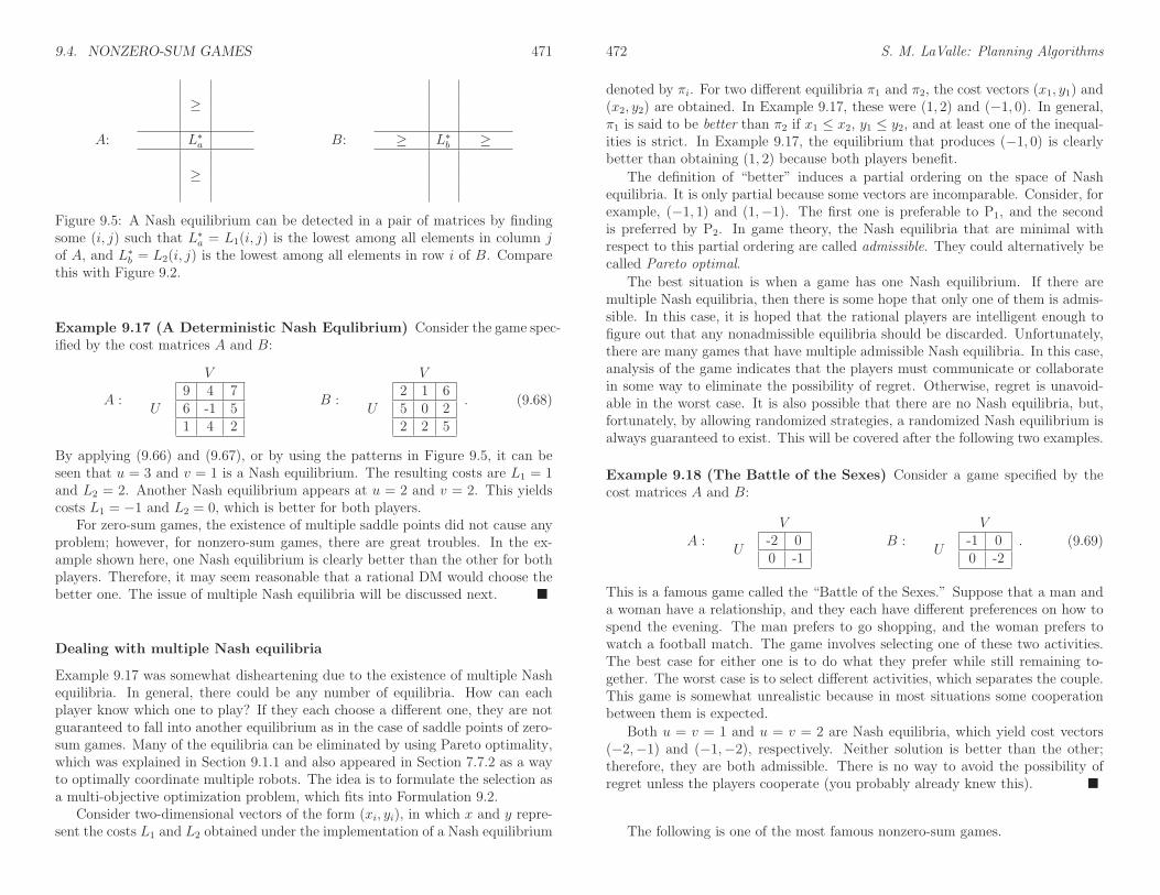
9.4. NONZERO-SUM GAMES 471
A:
≥
L∗
a
≥
B: ≥ L∗
b ≥
Figure 9.5: A Nash equilibrium can be detected in a pair of matrices by findingsome (i, j) such that L∗
a = L1(i, j) is the lowest among all elements in column jof A, and L∗
b = L2(i, j) is the lowest among all elements in row i of B. Comparethis with Figure 9.2.
Example 9.17 (A Deterministic Nash Equlibrium) Consider the game spec-ified by the cost matrices A and B:
A :
V
U9 4 76 -1 51 4 2
B :
V
U2 1 65 0 22 2 5
. (9.68)
By applying (9.66) and (9.67), or by using the patterns in Figure 9.5, it can beseen that u = 3 and v = 1 is a Nash equilibrium. The resulting costs are L1 = 1and L2 = 2. Another Nash equilibrium appears at u = 2 and v = 2. This yieldscosts L1 = −1 and L2 = 0, which is better for both players.
For zero-sum games, the existence of multiple saddle points did not cause anyproblem; however, for nonzero-sum games, there are great troubles. In the ex-ample shown here, one Nash equilibrium is clearly better than the other for bothplayers. Therefore, it may seem reasonable that a rational DM would choose thebetter one. The issue of multiple Nash equilibria will be discussed next.
Dealing with multiple Nash equilibria
Example 9.17 was somewhat disheartening due to the existence of multiple Nashequilibria. In general, there could be any number of equilibria. How can eachplayer know which one to play? If they each choose a different one, they are notguaranteed to fall into another equilibrium as in the case of saddle points of zero-sum games. Many of the equilibria can be eliminated by using Pareto optimality,which was explained in Section 9.1.1 and also appeared in Section 7.7.2 as a wayto optimally coordinate multiple robots. The idea is to formulate the selection asa multi-objective optimization problem, which fits into Formulation 9.2.
Consider two-dimensional vectors of the form (xi, yi), in which x and y repre-sent the costs L1 and L2 obtained under the implementation of a Nash equilibrium
472 S. M. LaValle: Planning Algorithms
denoted by πi. For two different equilibria π1 and π2, the cost vectors (x1, y1) and(x2, y2) are obtained. In Example 9.17, these were (1, 2) and (−1, 0). In general,π1 is said to be better than π2 if x1 ≤ x2, y1 ≤ y2, and at least one of the inequal-ities is strict. In Example 9.17, the equilibrium that produces (−1, 0) is clearlybetter than obtaining (1, 2) because both players benefit.
The definition of “better” induces a partial ordering on the space of Nashequilibria. It is only partial because some vectors are incomparable. Consider, forexample, (−1, 1) and (1,−1). The first one is preferable to P1, and the secondis preferred by P2. In game theory, the Nash equilibria that are minimal withrespect to this partial ordering are called admissible. They could alternatively becalled Pareto optimal.
The best situation is when a game has one Nash equilibrium. If there aremultiple Nash equilibria, then there is some hope that only one of them is admis-sible. In this case, it is hoped that the rational players are intelligent enough tofigure out that any nonadmissible equilibria should be discarded. Unfortunately,there are many games that have multiple admissible Nash equilibria. In this case,analysis of the game indicates that the players must communicate or collaboratein some way to eliminate the possibility of regret. Otherwise, regret is unavoid-able in the worst case. It is also possible that there are no Nash equilibria, but,fortunately, by allowing randomized strategies, a randomized Nash equilibrium isalways guaranteed to exist. This will be covered after the following two examples.
Example 9.18 (The Battle of the Sexes) Consider a game specified by thecost matrices A and B:
A :
V
U-2 00 -1
B :
V
U-1 00 -2
. (9.69)
This is a famous game called the “Battle of the Sexes.” Suppose that a man anda woman have a relationship, and they each have different preferences on how tospend the evening. The man prefers to go shopping, and the woman prefers towatch a football match. The game involves selecting one of these two activities.The best case for either one is to do what they prefer while still remaining to-gether. The worst case is to select different activities, which separates the couple.This game is somewhat unrealistic because in most situations some cooperationbetween them is expected.
Both u = v = 1 and u = v = 2 are Nash equilibria, which yield cost vectors(−2,−1) and (−1,−2), respectively. Neither solution is better than the other;therefore, they are both admissible. There is no way to avoid the possibility ofregret unless the players cooperate (you probably already knew this).
The following is one of the most famous nonzero-sum games.

9.4. NONZERO-SUM GAMES 473
Example 9.19 (The Prisoner’s Dilemma) The following game is very simpleto express, yet it illustrates many interesting issues. Imagine that a heinous crimehas been committed by two people. The authorities know they are guilty, butthey do not have enough evidence to convict them. Therefore, they develop aplan to try to trick the suspects. Each suspect (or player) is placed in an isolatedprison cell and given two choices. Each player can cooperate with the authorities,u = 1 or v = 1, or refuse, u = 2 or v = 2. By cooperating, the player admitsguilt and turns over evidence to the authorities. By refusing, the player claimsinnocence and refuses to help the authorities.
The cost Li represents the number of years that the player will be sentencedto prison. The cost matrices are assigned as
A :
V
U8 030 2
B :
V
U8 300 2
. (9.70)
The motivation is that both players receive 8 years if they both cooperate, which isthe sentence for being convicted of the crime and being rewarded for cooperatingwith the authorities. If they both refuse, then they receive 2 years because theauthorities have insufficient evidence for a longer term. The interesting casesoccur if one refuses and the other cooperates. The one who refuses is in bigtrouble because the evidence provided by the other will be used against him. Theone who cooperates gets to go free (the cost is 0); however, the other is convictedon the evidence and spends 30 years in prison.
What should the players do? What would you do? If they could make acoordinated decision, then it seems that a good choice would be for both to refuse,which results in costs (2, 2). In this case, however, there would be regret becauseeach player would think that he had a chance to go free (receiving cost 0 byrefusing). If they were to play the game a second time, they might be inclined tochange their decisions.
The Nash equilibrium for this problem is for both of them to cooperate, whichresults in (8, 8). Thus, they pay a price for not being able to communicate andcoordinate their strategy. This solution is also a security strategy for the players,because it achieves the lowest cost using worst-case analysis.
Randomized Nash equilibria
What happens if a game has no Nash equilibrium over the space of deterministicstrategies? Once again the problem can be alleviated by expanding the strategyspace to include randomized strategies. In Section 9.3.3 it was explained thatevery zero-sum game under Formulation 9.7 has a randomized saddle point onthe space of randomized strategies. It was shown by Nash that every nonzero-sum game under Formulation 9.8 has a randomized Nash equilibrium [29]. This
474 S. M. LaValle: Planning Algorithms
is a nice result; however, there are a couple of concerns. There may still existother admissible equilibria, which means that there is no reliable way to avoidregret unless the players collaborate. The other concern is that randomized Nashequilibria unfortunately cannot be computed using the linear programming ap-proach of Section 9.3.3. The required optimization is instead a form of nonlinearprogramming [6, 24, 30], which does not necessarily admit a nice, combinatorialsolution.
Recall the definition of randomized strategies from Section 9.3.3. For a pair(w, z) of randomized strategies, the expected costs, L1(w, z) and L2(w, z), can becomputed using (9.57). A pair (w∗, z∗) of strategies is said to be a randomizedNash equilibrium if
L1(w∗, z∗) = minw∈W
L1(w, z∗)
(9.71)
and
L2(w∗, z∗) = minz∈Z
L2(w∗, z)
. (9.72)
In game-theory literature, this is usually referred to as a mixed Nash equilibrium.Note that (9.71) and (9.72) are just generalizations of (9.66) and (9.67) from thespace of deterministic strategies to the space of randomized strategies.
Using the cost matrices A and B, the Nash equilibrium conditions can bewritten as
w∗Az∗ = minw∈W
wAz∗
(9.73)
and
w∗Bz∗ = minz∈Z
w∗Bz
. (9.74)
Unfortunately, the computation of randomized Nash equilibria is considerablymore challenging than computing saddle points. The main difficulty is that Nashequilibria are not necessarily security strategies. By using security strategies, it ispossible to decouple the decisions of the players into separate linear programmingproblems, as was seen in Example 9.16. For the randomized Nash equilibrium, theoptimization between the players remains coupled. The resulting optimization isoften referred to as the linear complementarity problem. This can be formulatedas a nonlinear programming problem [24, 30], which means that it is a nonlinearoptimization that involves both equality and inequality constraints on the domain(in this particular case, a bilinear programming problem is obtained [3]).
Example 9.20 (Finding a Randomized Nash Equilibrium) To get an ideaof the kind of optimization that is required, recall Example 9.18. A randomizedNash equilibrium that is distinct from the two deterministic equilibria can befound. Using the cost matrices from Example 9.18, the expected cost for P1 given

9.4. NONZERO-SUM GAMES 475
randomized strategies w and z is
L1(w, z) = wAz
=(
w1 w2
)
(
−2 00 −1
)(
z1z2
)
=− 2w1z1 − w2z2
=− 3w1z1 + w1 + z1,
(9.75)
in which the final step uses the fact that w2 = 1− w1 and z2 = 1− z1. Similarly,the expected cost for P2 is
L2(w, z) = wBz
=(
w1 w2
)
(
−1 00 −2
)(
z1z2
)
=− w1z1 − 2w2z2
=− 3w1z1 + 2w1 + 2z1.
(9.76)
If z is fixed, then the final equation in (9.75) is linear in w; likewise, if w isfixed, then (9.76) is linear in z. In the case of computing saddle points for zero-sum games, we were allowed to make this assumption; however, it is not possiblehere. We must choose (w∗, z∗) to simultaneously optimize (9.75) while z = z∗ and(9.76) while w = w∗.
It turns out that this problem is simple enough to solve with calculus. Usingthe classical optimization method of taking derivatives, a candidate solution canbe found by computing
∂L1(w1, z1)
∂w1
= 1− 3z1 (9.77)
and∂L2(w1, z1)
∂z1= 2− 3w1. (9.78)
Extrema occur when both of these simultaneously become 0. Solving 1− 3z1 = 0and 2− 3w1 = 0 yields (w∗, z∗) = (2/3, 1/3), which is a randomized Nash equilib-rium. The deterministic Nash equilibria are not detected by this method becausethey occur on the boundary of W and Z, where the derivative is not defined.
The computation method in Example 9.20 did not appear too difficult becausethere were only two actions per player, and half of the matrix costs were 0. In gen-eral, two complicated equations must be solved simultaneously. The expressions,however, are always second-degree polynomials. Furthermore, they each becomelinear with respect to the other variables if w or z is held fixed.
476 S. M. LaValle: Planning Algorithms
Summary of possible solutions The solution possibilities to remember for anonzero-sum game under Formulation 9.8 are as follows.
1. There may be multiple, admissible (deterministic) Nash equilibria.
2. There may be no (deterministic) Nash equilibria.
3. There is always at least one randomized Nash equilibrium.
9.4.2 More Than Two Players
The ideas of Section 9.4.1 easily generalize to any number of players. The maindifficulty is that complicated notation makes the concepts appear more difficult.Keep in mind, however, that there are no fundamental differences. A nonzero-sumgame with n players is formulated as follows.
Formulation 9.9 (An n-Player Nonzero-Sum Game)
1. A set of n players, P1, P2, . . ., Pn.
2. For each player Pi, a finite, nonempty set U i called the action space for Pi.For convenience, assume that each U i is a set of consecutive integers from 1to |U i|. Each ui ∈ U i is referred to as an action of Pi.
3. For each player Pi, a function, Li : U1 × U2 × · · · × Un → R ∪ ∞ called
the cost function for Pi.
A matrix formulation of the costs is no longer possible because there are too manydimensions. For example, if n = 3 and |U i| = 2 for each player, then Li(u
1, u2, u3)is specified by a 2 × 2 × 2 cube of 8 entries. Three of these cubes are needed tospecify the game. Thus, it may be helpful to just think of Li as a multivariatefunction and avoid using matrices.4
The Nash equilibrium idea generalizes by requiring that each Pi experiencesno regret, given the actions chosen by the other n − 1 players. Formally, a set(u1∗, . . . , un∗) of actions is said to be a (deterministic) Nash equilibrium if
Li(u1∗, . . . , ui∗, . . . , un∗) = min
ui∈U i
Li(u1∗, . . . , u(i−1)∗, ui, u(i+1)∗, . . . , un∗)
(9.79)
for every i ∈ 1, . . . , n.For n > 2, any of the situations summarized at the end of Section 9.4.1 can
occur. There may be no deterministic Nash equilibria or multiple Nash equilib-ria. The definition of an admissible Nash equilibrium is extended by defining thenotion of better over n-dimensional cost vectors. Once again, the minimal vectors
4If you enjoy working with tensors, these could be used to capture n-player cost functions[7].

9.4. NONZERO-SUM GAMES 477
with respect to the resulting partial ordering are considered admissible (or Paretooptimal). Unfortunately, multiple admissible Nash equilibria may still exist.
It turns out that for any game under Formulation 9.9, there exists a randomizedNash equilibrium. Let zi denote a randomized strategy for Pi. The expected costfor each Pi can be expressed as
Li(z1, z2, . . . , zn) =
m1∑
i1=1
m2∑
i2=1
· · ·mn∑
in=1
Li(i1, i2, . . . , in)z1i1z2i2 · · · znin . (9.80)
Let Zi denote the space of randomized strategies for Pi. An assignment,(z1∗, . . . , zn∗), of randomized strategies to all of the players is called a randomizedNash equilibrium if
Li(z1∗, . . . , zi∗, . . . , zn∗) = minzi∈Zi
Li(z1∗, . . . , z(i−1)∗, zi, z(i+1)∗, . . . , zn∗)
(9.81)
for all i ∈ 1, . . . , n.As might be expected, computing a randomized Nash equilibrium for n > 2
is even more challenging than for n = 2. The method of Example 9.20 can begeneralized to n-player games; however, the expressions become even more com-plicated. There are n equations, each of which appears linear if the randomizedstrategies are fixed for the other n−1 players. The result is a collection of n-degreepolynomials over which n optimization problems must be solved simultaneously.
Example 9.21 (A Three-Player Nonzero-Sum Game) Suppose there are threeplayers, P1, P2, and P3, each of which has two actions, 1 and 2. A deterministicstrategy is specified by a vector such as (1, 2, 1), which indicates u1 = 1, u2 = 2,and u3 = 1.
Now some costs will be defined. For convenience, let
L(i, j, k) =(
L1(i, j, k), L2(i, j, k), L3(i, j, k))
(9.82)
for each i, j, k ∈ 1, 2. Let the costs be
L(1, 1, 1) = (1, 1,−2) L(1, 1, 2) = (−4, 3, 1)
L(1, 2, 1) = (2,−4, 2) L(1, 2, 2) = (−5,−5, 10) (9.83)
L(2, 1, 1) = (3,−2,−1) L(2, 1, 2) = (−6,−6, 12)
L(2, 2, 1) = (2, 2,−4) L(2, 2, 2) = (−2, 3,−1).
There are two deterministic Nash equilibria, which yield the costs (2,−4, 2) and(3,−2,−1). These can be verified using (9.79). Each player is satisfied with theoutcome given the actions chosen by the other players. Unfortunately, both Nashequilibria are both admissible. Therefore, some collaboration would be neededbetween the players to ensure that no regret will occur.
478 S. M. LaValle: Planning Algorithms
9.5 Decision Theory Under Scrutiny
Numerous models for decision making were introduced in this chapter. Theseprovide a foundation for planning under uncertainty, which is the main focus ofPart III. Before constructing planning models with this foundation, it is importantto critically assess how appropriate it may be in applications. You may have hadmany questions while reading Sections 9.1 to 9.4. How are the costs determined?Why should we believe that optimizing the expected cost is the right thing to do?What happens if prior probability distributions are not available? Is worst-caseanalysis too conservative? Can we be sure that players in a game will followthe assumed rational behavior? Is it realistic that players know each other’scost functions? The purpose of this section is to help shed some light on thesequestions. A building is only as good as its foundation. Any mistakes made bymisunderstanding the limitations of decision theory will ultimately work their wayinto planning formulations that are constructed from them.
9.5.1 Utility Theory and Rationality
This section provides some justification for using cost functions and then minimiz-ing their expected value under Formulations 9.3 and 9.4. The resulting frameworkis called utility theory, which is usually formulated using rewards instead of costs.As stated in Section 9.1.1, a cost can be converted into a reward by multiplying by−1 and then swapping each maximization with minimization. We will thereforetalk about a reward R with the intuition that a higher reward is better.
Comparing rewards
Imagine assigning reward values to various outcomes of a decision-making pro-cess. In some applications numerical values may come naturally. For example,the reward might be the amount of money earned in a financial investment. Inrobotics applications, one could negate time to execute a task or the amount of en-ergy consumed. For example, the reward could indicate the amount of remainingbattery life after a mobile robot builds a map.
In some applications the source of rewards may be subjective. For example,what is the reward for washing dishes, in comparison to sweeping the floor? Eachperson would probably assign different rewards, which may even vary from dayto day. It may be based on their enjoyment or misery in performing the task,the amount of time each task would take, the perceptions of others, and so on.If decision theory is used to automate the decision process for a human “client,”then it is best to consult carefully with the client to make sure you know theirpreferences. In this situation, it may be possible to sort their preferences and thenassign rewards that are consistent with the ordering.
Once the rewards are assigned, consider making a decision under Formulation9.1, which does not involve nature. Each outcome corresponds directly to an

9.5. DECISION THEORY UNDER SCRUTINY 479
action, u ∈ U . If the rewards are given by R : U → R, then the cost, L, can bedefined as L(u) = −R(u) for every u ∈ U . Satisfying the client is then a matterof choosing u to minimize L.
Now consider a game against nature. The decision now involves comparingprobability distributions over the outcomes. The space of all probability distri-butions may be enormous, but this is simplified by using expectation to mapeach probability distribution (or density) to a real value. The concern should bewhether this projection of distributions onto real numbers will fail to reflect thetrue preferences of the client. The following example illustrates the effect of this.
Example 9.22 (Do You Like to Gamble?) Suppose you are given three choices:
1. You can have 1000 Euros.
2. We will toss an unbiased coin, and if the result is heads, then you will receive2000 Euros. Otherwise, you receive nothing.
3. With probability 2/3, you can have 3000 Euros; however, with probability1/3, you have to give me 3000 Euros.
The expected reward for each of these choices is 1000 Euros, but would you reallyconsider these to be equivalent? Your love or disdain for gambling is not beingtaken into account by the expectation. How should such an issue be consideredin games against nature?
To begin to fix this problem, it is helpful to consider another scenario. Manypeople would probably agree that having more money is preferable (if having toomuch worries you, then you can always give away the surplus to your favorite char-ities). What is interesting, however, is that being wealthy decreases the perceivedvalue of money. This is illustrated in the next example.
Example 9.23 (Reality Television) Suppose you are lucky enough to appearon a popular reality television program. The point of the show is to test how faryou will go in making a fool out of yourself, or perhaps even torturing yourself,to earn some money. You are asked to do some unpleasant task (such as eatingcockroaches, or holding your head under water for a long time, and so on.). Letu1 be the action to agree to do the task, and let u2 mean that you decline theopportunity. The prizes are expressed in U.S. dollars. Imagine that you are astarving student on a tight budget.
Below are several possible scenarios that could be presented on the televisionprogram. Consider how you would react to each one.
1. Suppose that u1 earns you $1 and u2 earns you nothing. Purely optimizingthe reward would lead to choosing u1, which means performing the unpleas-ant task. However, is this worth $1? The problem so far is that we are not
480 S. M. LaValle: Planning Algorithms
taking into account the amount of discomfort in completing a task. Perhapsit might make sense to make a reward function that shifts the dollar valuesby subtracting the amount for which you would be just barely willing toperform the task.
2. Suppose that u1 earns you $10,000 and u2 earns you nothing. $10,000 isassumed to be an enormous amount of money, clearly worth enduring anytorture inflicted by the television program. Thus, u1 is preferable.
3. Now imagine that the television host first gives you $10 million just forappearing on the program. Are you still willing to perform the unpleasanttask for an extra $10,000? Probably not. What is happening here? Yoursense of value assigned to money seems to decrease as you get more of it,right? It would not be too interesting to watch the program if the contestantswere all wealthy oil executives.
4. Suppose that you have performed the task and are about to win the prize.Just to add to the drama, the host offers you a gambling opportunity. Youcan select action u1 and receive $10,000, or be a gambler by selecting u2and have probability 1/2 of winning $25,000 by the tossing of a fair coin.In terms of the expected reward, the clear choice is u2. However, you justcompleted the unpleasant task and expect to earn money. The risk of losingit all may be intolerable. Different people will have different preferences inthis situation.
5. Now suppose once again that you performed the task. This time your choicesare u1, to receive $100, or u2, to have probability 1/2 of receiving $250 bytossing a fair coin. The host is kind enough, though, to let you play 100times. In this case, the expected totals for the two actions are $10,000 and$12,500, respectively. This time it seems clear that the best choice is to gam-ble. After 100 independent trials, we would expect that, with extremely highprobability, over $10,000 would be earned. Thus, reasoning by expected-caseanalysis seems valid if we are allowed numerous, independent trials. In thiscase, with high probability a value close to the expected reward should bereceived.
Based on these examples, it seems that the client or evaluator of the decision-making system must indicate preferences between probability distributions overoutcomes. There is a formal way to ensure that once these preferences are assigned,a cost function can be designed for which its expectation faithfully reflects thepreferences over distributions. This results in utility theory, which involves thefollowing steps:

9.5. DECISION THEORY UNDER SCRUTINY 481
1. Require that the client is rational when assigning preferences. This notionis defined through axioms.
2. If the preferences are assigned in a way that is consistent with the axioms,then a utility function is guaranteed to exist. When expected utility isoptimized, the preferences match exactly those of the client.
3. The cost function can be derived from the utility function.
The client must specify preferences among probability distributions of out-comes. Suppose that Formulation 9.2 is used. For convenience, assume that U andΘ are finite. Let X denote a state space based on outcomes.5 Let f : U ×Θ → Xdenote a mapping that assigns a state to every outcome. A simple example is todeclare that X = U × Θ and make f the identity map. This makes the outcomespace and state space coincide. It may be convenient, though, to use f to collapsethe space of outcomes down to a smaller set. If two outcomes map to the samestate using f , then it means that the outcomes are indistinguishable as far asrewards or costs are concerned.
Let z denote a probability distribution over X, and let Z denote the set of allprobability distributions over X. Every z ∈ Z is represented as an n-dimensionalvector of probabilities in which n = |X|; hence, it is considered as an element of Rn.This makes it convenient to “blend” two probability distributions. For example,let α ∈ (0, 1) be a constant, and let z1 and z2 be any two probability distributions.Using scalar multiplication, a new probability distribution, αz1 + (1 − α)z2, isobtained, which is a blend of z1 and z2. Conveniently, there is no need to normalizethe result. It is assumed that z1 and z2 initially have unit magnitude. The blendhas magnitude α + (1− α) = 1.
The modeler of the decision process must consult the client to represent pref-erences among elements of Z. Let z1 ≺ z2 mean that z2 is strictly preferred overz1. Let z1 ≈ z2 mean that z1 and z2 are equivalent in preference. Let z1 z2 meanthat either z1 ≺ z2 or z1 ≈ z2. The following example illustrates the assignmentof preferences.
Example 9.24 (Indicating Preferences) Suppose that U = Θ = 1, 2, whichleads to four possible outcomes: (1, 1), (1, 2), (2, 1), and (2, 2). Imagine that na-ture represents a machine that generates 1 or 2 according to a probability distri-bution. The action is to guess the number that will be generated by the machine.If you pick the same number, then you win that number of gold pieces. If you donot pick the same number, then you win nothing, but also lose nothing.
Consider the construction of the state space X by using f . The outcomes(2, 1) and (1, 2) are identical concerning any conceivable reward. Therefore, theseshould map to the same state. The other two outcomes are distinct. The statespace therefore needs only three elements and can be defined as X = 0, 1, 2.
5In most utility theory literature, this is referred to as a reward space, R [5].
482 S. M. LaValle: Planning Algorithms
Let f(2, 1) = f(1, 2) = 0, f(1, 1) = 1, and f(2, 2) = 2. Thus, the last two statesindicate that some gold will be earned.
The set Z of probability distributions over X is now considered. Each z ∈ Z isa three-dimensional vector. As an example, z1 = [1/2 1/4 1/4] indicates that thestate will be 0 with probability 1/2, 1 with probability 1/4, and 2 with probability1/4. Suppose z2 = [1/3 1/3 1/3]. Which distribution would you prefer? It seemsin this case that z2 is uniformly better than z1 because there is a greater chanceof winning gold. Thus, we declare z1 ≺ z2. The distribution z3 = [1 0 0] seemsto be the worst imaginable. Hence, we can safely declare z3 ≺ z1 and z1 ≺ z2.
The procedure of determining the preferences can become quite tedious forcomplicated problems. In the current example, Z is a 2D subset of R3. Thissubset can be partitioned into a finite set of regions over which the client may beable to clearly indicate preferences. One of the major criticisms of this frameworkis the impracticality of determining preferences over Z [34].
After the preferences are determined, is there a way to ensure that a real-valuefunction on X exists for which the expected value exactly reflects the preferences?If the axioms of rationality are satisfied by the assignment of preferences, thenthe answer is yes. These axioms are covered next.
Axioms of rationality
To meet the goal of designing a utility function, it turns out that the preferencesmust follow rules called the axioms of rationality. They are sensible statementsof consistency among the preferences. As long as these are followed, then a util-ity function is guaranteed to exist (detailed arguments appear in [14, 34]). Thedecision maker is considered rational if the following axioms are followed whendefining ≺ and ≈:6
1. If z1, z2 ∈ Z, then either z1 z2 or z2 z1.“You must be able to make up your mind.”
2. If z1 z2 and z2 z3, then z1 z3.“Preferences must be transitive.”
3. If z1 ≺ z2, thenαz1 + (1− α)z3 ≺ αz2 + (1− α)z3, (9.84)
for any z3 ∈ Z and α ∈ (0, 1).“Evenly blending in a new distribution does not alter preference.”
4. If z1 ≺ z2 ≺ z3, then there exists some α ∈ (0, 1) and β ∈ (0, 1) such that
αz1 + (1− α)z3 ≺ z2 (9.85)
6Alternative axiom systems exist [14, 36].

9.5. DECISION THEORY UNDER SCRUTINY 483
andz2 ≺ βz1 + (1− β)z3. (9.86)
“There is no heaven or hell.”
Each axiom has an intuitive interpretation that makes practical sense. The firstone simply indicates that the preference direction can always be inferred for a pairof distributions. The second axiom indicates that preferences must be transitive.7
The last two axioms are somewhat more complicated. In the third axiom, z2 isstrictly preferred to z1. An attempt is made to cause confusion by blending in athird distribution, z3. If the same “amount” of z3 is blended into both z1 and z2,then the preference should not be affected. The final axiom involves z1, z2, andz3, each of which is strictly better than its predecessor. The first equation, (9.85),indicates that if z2 is strictly better than z1, then a tiny amount of z3 can beblended into z1, with z2 remaining preferable. If z3 had been like “heaven” (i.e.,infinite reward), then this would not be possible. Similarly, (9.86) indicates thata tiny amount of z1 can be blended into z3, and the result remains better than z2.This means that z1 cannot be “hell,” which would have infinite negative reward.8
Constructing a utility function
If the preferences have been determined in a way consistent with the axioms, thenit can be shown that a utility function always exists. This means that there existsa function U : X → R such that, for all z1, z2 ∈ Z,
z1 ≺ z2 if and only if Ez1 [U ] < Ez2 [U ], (9.87)
in which Ezi denotes the expected value of U , which is being treated as a randomvariable under the probability distribution zi. The existence of U implies that itis safe to determine the best action by maximizing the expected utility.
A reward function can be defined using a utility function, U , as R(u, θ) =U(f(u, θ)). The utility function can be converted to a cost function as L(u, θ) =−R(u, θ) = −U(f(u, θ)). Minimizing the expected cost, as was recommendedunder Formulations 9.3 and 9.4 with probabilistic uncertainty, now seems justifiedunder the assumption that U was constructed correctly to preserve preferences.
Unfortunately, establishing the existence of a utility function does not producea systematic way to construct it. In most circumstances, one is forced to design Uby a trial-and-error process that involves repeatedly checking the preferences. Inthe vast majority of applications, people create utility and cost functions withoutregard to the implications discussed in this section. Thus, undesirable conclusions
7For some reasonable problems, however, transitivity is not desirable. See the Candorcet andSimpson paradoxes in [34].
8Some axiom systems allow infinite rewards, which lead to utility and cost functions withinfinite values, but this is not considered here.
484 S. M. LaValle: Planning Algorithms
U(x)
x
Figure 9.6: The utility of new amounts of money decreases as the total accumu-lation of wealth increases. The utility function may even bounded.
may be reached in practice. Therefore, it is important not to be too confidentabout the quality of an optimal decision rule.
Note that if worst-case analysis had been used, then most of the problemsdiscussed here could have been avoided. Worst-case analysis, however, has itsweaknesses, which will be discussed in Section 9.5.3.
Example 9.25 (The Utility of Money) We conclude the section by depictinga utility function that is often applied to money. Suppose that the state spaceX = R, which corresponds to the amount of U.S. dollars earned. The utilityof money applied by most people indicates that the value of new increments ofmoney decreases as the total accumulated wealth increases. The utility functionmay even be bounded. Imagine there is some maximum dollar amount, such as$10100, after which additional money has no value. A typical utility curve is shownin Figure 9.6 [5].
9.5.2 Concerns Regarding the Probabilistic Model
Section 9.5.1 addressed the source of cost functions and the validity of takingtheir expectations. This section raises concerns over the validity of the probabilitydistributions used in Section 9.2. The two main topics are criticisms of Bayesianmethods in general and problems with constructing probability distributions.
Bayesians vs. frequentists
For the past century and a half, there has been a fundamental debate amongstatisticians on the meaning of probabilities. Virtually everyone is satisfied withthe axioms of probability, but beyond this, what is their meaning when makinginferences? The two main camps are the frequentists and the Bayesians. A formof Bayes’ rule was published in 1763 after the death of Bayes [4]. During most ofthe nineteenth century Bayesian analysis tended to dominate literature; however,

9.5. DECISION THEORY UNDER SCRUTINY 485
during the twentieth century, the frequentist philosophy became more popular asa more rigorous interpretation of probabilities. In recent years, the credibility ofBayesian methods has been on the rise again.
As seen so far, a Bayesian interprets probabilities as the degree of belief ina hypothesis. Under this philosophy, it is perfectly valid to begin with a priordistribution, gather a few observations, and then make decisions based on theresulting posterior distribution from applying Bayes’ rule.
From a frequentist perspective, Bayesian analysis makes far too liberal useof probabilities. The frequentist believes that probabilities are only defined asthe quantities obtained in the limit after the number of independent trials tendsto infinity. For example, if an unbiased coin is tossed over numerous trials, theprobability 1/2 represents the value to which the ratio between heads and the totalnumber of trials will converge as the number of trials tends to infinity. On theother hand, a Bayesian might say that the probability that the next trial resultsin heads is 1/2. To a frequentist, this interpretation of probability is too strong.
Frequentists have developed a version of decision theory based on their philos-ophy; comparisons between the two appear in [34]. As an example, a frequentistwould advocate optimizing the following frequentist risk to obtain a decision rule:
R(θ, π) =
∫
y
L(π(y), θ)P (y|θ)dy, (9.88)
in which π represents the strategy, π : Y → U . The frequentist risk averages overall data, rather than making a decision based on a single observation, as advocatedby Bayesians in (9.26). The probability P (y|θ) is assumed to be obtained inthe limit as the number of independent data trials tends to infinity. The maindrawback in using (9.88) is that the optimization depends on θ. The resultingbest decision rule must depend on θ, which is unknown. In some limited cases, itmay be possible to select some π that optimizes (9.88) for all θ, but this rarelyoccurs. Thus, the frequentist risk can be viewed as a constraint on the desirabilityof strategies, but it usually is not powerful enough to select a single one. Thisproblem is reminiscent of Pareto optimality, which was discussed in Section 9.1.1.The frequentist approach attempts to be more conservative and rigorous, with theresult being that weaker statements are made regarding decisions.
The source of prior distributions
Suppose that the Bayesian method has been adopted. The most widespread con-cern in all Bayesian analyses is the source of the prior distribution. In Section9.2, this is represented as P (θ) (or p(θ)), which represents a distribution (or den-sity) over the nature action space. The best way to obtain P (θ) is by estimatingthe distribution over numerous independent trials. This brings its definition intoalignment with frequentist views. This was possible with Example 9.11, in whichP (θ) could be reliably estimated from the frequency of occurrence of letters across
486 S. M. LaValle: Planning Algorithms
numerous pages of text. The distribution could even be adapted to a particularlanguage or theme.
In most applications that use decision theory, however, it is impossible or toocostly to perform such experiments. What should be done in this case? If a priordistribution is simply “made up,” then the resulting posterior probabilities maybe suspect. In fact, it may be invalid to call them probabilities at all. Sometimesthe term subjective probabilities is used in this case. Nevertheless, this is com-monly done because there are few other options. One of these options is to resortto frequentist decision theory, but, as mentioned, it does not work with singleobservations.
Fortunately, as the number of observations increases, the influence of the prioron the Bayesian posterior distributions diminishes. If there is only one observation,or even none as in Formulation 9.3, then the prior becomes very influential. Ifthere is little or no information regarding P (θ), the distribution should be designedas carefully as possible. It should also be understood that whatever conclusionsare made with this assumption, they are biased by the prior. Suppose this modelis used as the basis of a planning approach. You might feel satisfied computing the“optimal” plan, but this notion of optimality could still depend on some arbitraryinitial bias due to the assignment of prior values.
If there is no information available, then it seems reasonable that P (θ) shouldbe as uniform as possible over Θ. This was referred to by Laplace as the “principleof insufficient reason” [23]. If there is no reason to believe that one element is morelikely than another, then they should be assigned equal values. This can also bejustified by using Shannon’s entropy measure from information theory [2, 10, 39].In the discrete case, this is
−∑
θ∈Θ
P (θ) lgP (θ), (9.89)
and in the continuous case it is
−∫
Θ
p(θ) lg p(θ)dθ. (9.90)
This entropy measure was developed in the context of communication systemsto estimate the minimum number of bits needed to encode messages deliveredthrough a noisy medium. It generally indicates the amount of uncertainty associ-ated with the distribution. A larger value of entropy implies a greater amount ofuncertainty.
It turns out that the entropy function is maximized when P (θ) is a uniformdistribution, which seems to justify the principle of insufficient reason. This can beconsidered as a noninformative prior. The idea is even applied quite frequentlywhen Θ = R, which leads to an improper prior. The density function cannotmaintain a constant, nonzero value over all of R because its integral would beinfinite. Since the decisions made in Section 9.2 do not depend on any normalizing

9.5. DECISION THEORY UNDER SCRUTINY 487
factors, a constant value can be assigned for p(θ) and the decisions are not affectedby the fact that the prior is improper.
The main difficulty with applying the entropy argument in the selection of aprior is that Θ itself may be chosen in a number of arbitrary ways. Uniform as-signments to different choices of Θ ultimately yield different information regardingthe priors. Consider the following example.
Example 9.26 (A Problem with Noninformative Priors) Consider a deci-sion about what activities to do based on the weather. Imagine that there isabsolutely no information about what kind of weather is possible. One possibleassignment is Θ = p, c, in which p means “precipitation” and c means “clear.”Maximizing (9.89) suggests assigning P (p) = P (c) = 1/2.
After thinking more carefully, perhaps we would like to distinguish between dif-ferent kinds of precipitation. A better set of nature actions would be Θ = r, s, c,in which c still means “clear,” but precipitation p has been divided into r for “rain”and s for “snow.” Now maximizing (9.89) assigns probability 1/3 to each natureaction. This is clearly different from the original assignment. Now that we distin-guish between different kinds of precipitation, it seems that precipitation is muchmore likely to occur. Does our preference to distinguish between different formsof precipitation really affect the weather?
Example 9.27 (Noninformitive Priors for Continuous Spaces) Similar trou-bles can result in continuous spaces. Recall the parameter estimation problemdescribed in Example 9.12. Suppose instead that the task is to estimate a linebased on some data points that were supposed to fall on the line but missed dueto noise in the measurement process.
What initial probability density should be assigned to Θ, the set of all lines?Suppose that the line lives in Z = R
2. The line equation can be expressed as
θ1z1 + θ2z2 + θ3 = 0. (9.91)
The problem is that if the parameter vector, θ = [θ1 θ2 θ3], is multiplied bya scalar constant, then the same line is obtained. Thus, even though θ ∈ R
3, aconstraint must be added. Suppose we require that
θ21 + θ22 + θ13 = 1 (9.92)
and θ1 ≥ 0. This mostly fixes the problem and ensures that each parameter valuecorresponds to a unique line (except for some duplicate cases at θ1 = 0, but thesecan be safely neglected here). Thus, the parameter space is the upper half of asphere, S2. The maximum-entropy prior suggests assigning a uniform probabilitydensity to Θ. This may feel like the right thing to do, but this notion of uniformityis biased by the particular constraint applied to the parameter space to ensureuniqueness. There are many other choices. For example, we could replace (9.92)
488 S. M. LaValle: Planning Algorithms
by constraints that force the points to lie on the upper half of the surface of cube,instead of a sphere. A uniform probability density assigned in this new parameterspace certainly differs from one over the sphere.
In some settings, there is a natural representation of the parameter space thatis invariant to certain transformations. Section 5.1.4 introduced the notion ofHaar measure. If the Haar measure is used as a noninformative prior, then ameaningful notion of uniformity may be obtained. For example, suppose thatthe parameter space is SO(3). Uniform probability mass over the space of unitquaternions, as suggested in Example 5.14, is an excellent choice for a noninfor-mative prior because it is consistent with the Haar measure, which is invariant togroup operations applied to the events. Unfortunately, a Haar measure does notexist for most spaces that arise in practice.9
Incorrect assumptions on conditional distributions
One final concern is that many times even the distribution P (y|θ) is incorrectlyestimated because it is assumed arbitrarily to belong to a family of distributions.For example, it is often very easy to work with Gaussian densities. Therefore, itis tempting to assume that p(y|θ) is Gaussian. Experiments can be performed toestimate the mean and variance parameters. Even though some best fit will befound, it does not necessarily imply that a Gaussian is a good representation. Con-clusions based on this model may be incorrect, especially if the true distributionhas a different shape, such as having a larger tail or being multimodal. In manycases, nonparametric methods may be needed to avoid such biases. Such methodsdo not assume a particular family of distributions. For example, imagine estimat-ing a probability distribution by making a histogram that records the frequencyof y occurrences for a fixed value of θ. The histogram can then be normalizedto contain a representation of the probability distribution without assuming aninitial form.
9.5.3 Concerns Regarding the Nondeterministic Model
Given all of the problems with probabilistic modeling, it is tempting to abandonthe whole framework and work strictly with the nondeterministic model. This onlyrequires specifying Θ, without indicating anything about the relative likelihoodsof various actions. Therefore, most of the complicated issues presented in Sections9.5.1 and 9.5.2 vanish. Unfortunately, this advantage comes at a substantial price.Making decisions with worst-case analysis under the nondeterministic model hasits own shortcomings. After considering the trade-offs, you can decide which ismost appropriate for a particular application of interest.
9A locally compact topological group is required [18, 35].

9.5. DECISION THEORY UNDER SCRUTINY 489
The first difficulty is to ensure that Θ is sufficiently large to cover all possi-bilities. Consider Formulation 9.6, in which nature acts twice. Through a natureobservation action space, Ψ(θ), interference is caused in the measurement process.Suppose that Θ = R and h(θ, ψ) = θ + ψ. In this case, Ψ(θ) can be interpretedas the measurement error. What is the maximum amount of error that can oc-cur? Perhaps a sonar is measuring the distance from the robot to a wall. Basedon the sensor specifications, it may be possible to construct a nice bound on theerror. Occasionally, however, the error may be larger than this bound. Sonarssometimes fail to hear the required echo to compute the distance. In this case thereported distance is ∞. Due to reflections, extremely large errors can sometimesoccur. Although such errors may be infrequent, if we want guaranteed perfor-mance, then large or even infinite errors should be included in Ψ(θ). The problemis that worst-case reasoning could always conclude that the sensor is useless byreporting ∞. Any statistically valid information that could be gained from thesensor would be ignored. Under the probabilistic model, it is easy to make Ψ(θ)quite large and then assign very small probabilities to larger errors. The prob-lem with nondeterministic uncertainty is that Ψ(θ) needs to be smaller to makeappropriate decisions; however, theoretically “guaranteed” performance may nottruly be guaranteed in practice.
Once a nondeterministic model is formulated, the optimal decision rule mayproduce results that seem absurd for the intended application. The problem isthat the DM cannot tolerate any risk. An action is applied only if the result canbe guaranteed. The hope of doing better than the worst case is not taken intoaccount. Consider the following example:
Example 9.28 (A Problem with Conservative Decision Making) Supposethat a friend offers you the choice of either a check for 1000 Euros or 1 Euro incash. With the check, you must take it to the bank, and there is a small chancethat your friend will have insufficient funds in the account. In this case, you willreceive nothing. If you select the 1 Euro in cash, then you are guaranteed to earnsomething.
The following cost matrix reflects the outcomes (ignoring utility theory):
U
Θ1 10001 0
. (9.93)
Using probabilistic analysis, we might conclude that it is best to take the check.Perhaps the friend is even known to be very wealthy and responsible with bank-ing accounts. This information, however, cannot be taken into account in thedecision-making process. Using worst-case analysis, the optimal action is to takethe 1 Euro in cash. You may not feel too good about it, though. Imagine theregret if you later learn that the account had sufficient funds to cash the checkfor 1000 Euros.
490 S. M. LaValle: Planning Algorithms
Thus, it is important to remember the price that one must pay for wanting re-sults that are absolutely guaranteed. The probabilistic model offers the flexibilityof incorporating statistical information. Sometimes the probabilistic model canbe viewed as a generalization of the nondeterministic model. If it is assumed thatnature acts after the robot, then the nature action can take this into account, asincorporated into Formulation 9.4. In the nondeterministic case, Θ(u) is speci-fied, and in the probabilistic case, P (θ|u) is specified. The distribution P (θ|u)can be designed so that nature selects with very high probability the θ ∈ Θ thatmaximizes L(u, θ). In Example 9.28, this would mean that the probability thatthe check would bounce (resulting in no earnings) would by very high, such as0.999999. In this case, even the optimal action under the probabilistic model isto select the 1 Euro in cash. For virtually any decision problem that is modeledusing worst-case analysis, it is possible to work backward and derive possible pri-ors for which the same decision would be made using probabilistic analysis. InExample 9.4, it seemed as if the decision was based on assuming that with veryhigh probability, the check would bounce, even though there were no probabilisticmodels.
This means that worst-case analysis under the nondeterministic model can beconsidered as a special case of a probabilistic model in which the prior distributionassigns high probabilities to the worst-case outcomes. The justification for thiscould be criticized in the same way that other prior assignments are criticized inBayesian analysis. What is the basis of this particular assignment?
9.5.4 Concerns Regarding Game Theory
One of the most basic limitations of game theory is that each player must know thecost functions of the other players. As established in Section 9.5.1, it is even quitedifficult to determine an appropriate cost function for a single decision maker. Itis even more difficult to determine costs and motivations of other players. In mostpractical settings this information is not available. One possibility is to modeluncertainty associated with knowledge of the cost function of another player.Bayesian analysis could be used to reason about the cost based on observations ofactions chosen by the player. Issues of assigning priors once again arise. One ofthe greatest difficulties in allowing uncertainties in the cost functions is that a kindof “infinite reflection” occurs [19]. For example, if I am playing a game, does theother player know my cost function? I may be uncertain about this. Furthermore,does the other player know that I do not completely know its cost function? Thiskind of second-guessing can occur indefinitely, leading to a nightmare of nestedreasoning and assignments of prior distributions.10
The existence of saddle points or Nash equilibria was assured by using ran-
10Readers familiar with the movie The Princess Bride may remember the humorous dialogbetween Vizzini and the Dread Pirate Roberts about which goblet contains the deadly Iocanepowder.

9.5. DECISION THEORY UNDER SCRUTINY 491
domized strategies. Mathematically, this appears to be a clean solution to a frus-trating problem; however, it also represents a substantial change to the model.Many games are played just once. For the expected-case results to converge, thegame must be played an infinite number of times. If a game is played once, oronly a few times, then the players are very likely to experience regret, even thoughthe theory based on expected-case analysis indicates that regret is eliminated.
Another issue is that intelligent human players may fundamentally alter theirstrategies after playing a game several times. It is very difficult for humans tosimulate a randomized strategy (assuming they even want to, which is unlikely).There are even international tournaments in which the players repeatedly engagein classic games such as Rock-Paper-Scissors or the Prisoner’s Dilemma. For aninteresting discussion of a tournament in which people designed programs thatrepeatedly compete on the Prisoner’s Dilemma, see [41]. It was observed thateven some cooperation often occurs after many iterations, which secures greaterrewards for both players, even though they cannot communicate. A famous strat-egy arose in this context called Tit-for-Tat (written by Anatol Rapoport), whichin each stage repeated the action chosen by the other player in the last stage. Theapproach is simple yet surprisingly successful.
In the case of nonzero-sum games, it is particularly disheartening that multipleNash equilibria may exist. Suppose there is only one admissible equilibrium amongseveral Nash equilibria. Does it really seem plausible that an adversary wouldthink very carefully about the various Nash equilibria and pick the admissibleone? Perhaps some players are conservative and even play security strategies,which completely destroys the assumptions of minimizing regret. If there aremultiple admissible Nash equilibria, it appears that regret is unavoidable unlessthere is some collaboration between players. This result is unfortunate if suchcollaboration is impossible.
Further Reading
Section 9.1 covered very basic concepts, which can be found in numerous books and onthe Internet. For more on Pareto optimality, see [38, 40, 42, 46]. Section 9.2 is inspiredmainly by decision theory books. An excellent introduction is [5]. Other sources include[14, 15, 25, 34]. The “game against nature” view is based mainly on [8]. Patternclassification, which is an important form of decision theory, is covered in [1, 15, 16, 28].Bayesian networks [32] are a popular representation in artificial intelligence researchand often provide compact encodings of information for complicated decision-makingproblems.
Further reading on the game theory concepts of Sections 9.3 and 9.4 can be foundin many books (e.g., [3, 31]). A fun book that has many examples and intuitions is [41].For games that have infinite action sets, see [3]. The computation of randomized Nashequilibria remains a topic of active research. A survey of methods appears in [26]; seealso [21, 27]. The coupled polynomial equations that appear in computing randomizedNash equilibria may seem to suggest applying algorithms from computational algebraic
492 S. M. LaValle: Planning Algorithms
geometry, as were needed in Section 6.4 to solve this kind of problem in combinatorialmotion planning. An approach that uses such tools is given in [12]. Contrary to thenoncooperative games defined in Section 9.4, cooperative game theory investigates waysin which various players can form coalitions to improve their rewards [33].
Parts of Section 9.5 were inspired by [5]. Utility theory appears in most decisiontheory books (e.g., [5]) and in some artificial intelligence books (e.g., [36]). An in-depthdiscussion of Bayesian vs. frequentist issues appears in [34]. For a thorough introductionto constructing cost models for decision making, see [20].
Exercises
1. Suppose that a single-stage two-objective decision-making problem is defined inwhich there are two objectives and a continuous set of actions, U = [−10, 10].The cost vector is L = [u2 u− 1]. Determine the set of Pareto-optimal actions.
2. Let
Θ
U
−1 3 2 −1
−1 0 7 −1
1 5 5 −2
define the cost for each combination of choices by the decision maker and nature.Let nature’s randomized strategy be [1/5 2/5 1/10 3/10].
(a) Use nondeterministic reasoning to find the minimax decision and worst-casecost.
(b) Use probabilistic reasoning to find the best expected-case decision and ex-pected cost.
3. Many reasonable decision rules are possible, other than those considered in thischapter.
(a) Exercise 2(a) reflects extreme pessimism. Suppose instead that extremeoptimism is used. Select the choice that optimizes the best-case cost for thematrix in Exercise 2.
(b) One approach is to develop a coefficient of optimism, α ∈ [0, 1], which allowsone to interpolate between the two extreme scenarios. Thus, a decision,u ∈ U , is chosen by minimizing
α maxθ∈Θ
L(u, θ)
+ (1− α) minθ∈Θ
L(u, θ)
. (9.94)
Determine the optimal decision for this scenario under all possible choicesfor α ∈ [0, 1]. Give your answer as a list of choices, each with a specifiedrange of α.

9.5. DECISION THEORY UNDER SCRUTINY 493
4. Suppose that after making a decision, you observe the choice made by nature. Howdoes the cost that you received compare with the best cost that could have beenobtained if you chose something else, given this choice by nature? This differencein costs can be considered as regret or minimum “Doh!”11 Psychologists haveargued that some people make choices based on minimizing regret. It reflectshow badly you wish you had done something else after making the decision.
(a) Develop an expression for the worst-case regret, and use it to make a mini-max regret decision using the matrix from Exercise 2.
(b) Develop an expression for the expected regret, and use it to make a minimumexpected regret decision.
5. Using the matrix from Exercise 2, consider the set of all probability distributionsfor nature. Characterize the set of all distributions for which the minimax decisionand the best expected decision results in the same choice. This indicates how toprovide reverse justification for priors.
6. Consider a Bayesian decision-theory scenario with cost function L. Show that thedecision rule never changes if L(u, θ) is replaced by aL(u, θ) + b, for any a > 0and b ∈ R.
7. Suppose that there are two classes, Ω = ω1, ω2, with P (ω1) = P (ω2) =12 . The
observation space, Y , is R. Recall from probability theory that the normal (orGaussian) probability density function is
p(y) =1
σ√2π
e−(y−µ)2/2σ2
, (9.95)
in which µ denotes the mean and σ2 denotes the variance. Suppose that p(y|ω1)is a normal density in which µ = 0 and σ2 = 1. Suppose that p(y|ω2) is anormal density in which µ = 6 and σ2 = 4. Find the optimal classification rule,γ : Y → Ω. You are welcome to solve the problem numerically (by computer) orgraphically (by careful function plotting). Carefully explain how you arrived atthe answer in any case.
8. Let
Θ
U
2 −2 −2 1
−1 −2 −2 6
4 0 −3 4
give the cost for each combination of choices by the decision maker and nature.Let nature’s randomized strategy be [1/4 1/2 1/8 1/8].
(a) Use nondeterministic reasoning to find the minimax decision and worst-casecost.
11In 2001, the Homer Simpson term“Doh!” was added to the Oxford English Dictionary asan expression of regret.
494 S. M. LaValle: Planning Algorithms
(b) Use probabilistic reasoning to find the best expected-case decision and ex-pected cost.
(c) Characterize the set of all probability distributions for which the minimaxdecision and the best expected decision results in the same choice.
9. In a constant-sum game, the costs for any u ∈ U and v ∈ V add to yield
L1(u, v) + L2(u, v) = c (9.96)
for some constant c that is independent of u and v. Show that any constant-sumgame can be transformed into a zero-sum game, and that saddle point solutionscan be found using techniques for the zero-sum formulation.
10. Formalize Example 9.7 as a zero-sum game, and compute security strategies forthe players. What is the expected value of the game?
11. Suppose that for two zero-sum games, there exists some nonzero c ∈ R for whichthe cost matrix of one game is obtained by multiplying all entries by c in the costmatrix of the other. Prove that these two games must have the same deterministicand randomized saddle points.
12. In the same spirit as Exercise 11, prove that two zero-sum games have the samedeterministic and randomized saddle points if c is added to all matrix entries.
13. Prove that multiple Nash equilibria of a nonzero-sum game specified by matricesA and B are interchangeable if (A,B) as a game yields the same Nash equilibriaas the game (A,−A).
14. Analyze the game of Rock-Paper-Scissors for three players. For each player, assigna cost of 1 for losing, 0 for a tie, and −1 for winning. Specify the cost functions.Is it possible to avoid regret? Does it have a deterministic Nash equilibrium? Canyou find a randomized Nash equilibrium?
15. Compute the randomized equilibrium point for the following zero-sum game:
V
U0 -1
-1 2
. (9.97)
Indicate the randomized strategies for the players and the resulting expected valueof the game.
Implementations
16. Consider estimating the value of an unknown parameter, θ ∈ R. The prior prob-ability density is a normal,
p(θ) =1
σ√2π
e−(θ−µ)2/2σ2
, (9.98)

9.5. DECISION THEORY UNDER SCRUTINY i
with µ = 0 and σ = 4. Suppose that a sequence, y1, y2, . . ., yk, of k observationsis made and that each p(yi|θ) is a normal density with µ = θ and σ = 9. Supposethat u represents your guess of the parameter value. The task is select u tominimize the expectation of the cost, L(u, θ) = (u− θ)2. Suppose that the “true”value of θ is 4. Determine the u∗, the minimal action with respect to the expectedcost after observing: yi = 4 for every i ∈ 1, . . . , k.
(a) Determine u∗ for k = 1.
(b) Determine u∗ for k = 10.
(c) Determine u∗ for k = 1000.
This experiment is not very realistic because the observations should be generatedby sampling from the normal density, p(yi|θ). Repeat the exercise using valuesdrawn with the normal density, instead of yk = 4, for each k.
17. Implement an algorithm that computes a randomized saddle point for zero-sumgames. Assume that one player has no more than two actions and the other mayhave any finite number of actions.
18. Suppose that a K-stage decision-making problem is defined using multiple objec-tives. There is a finite state space X and a finite action set U(x) for each x ∈ X.A state transition equation, xk+1 = f(xk, uk), gives the next state from a currentstate and input. There are N cost functionals of the form
Li(u1, . . . , uK) =K∑
k=1
l(xk, uk) + lF (xF ), (9.99)
in which F = K+1. Assume that lF (xF ) = ∞ if xF ∈ Xgoal (for some goal regionXgoal ⊂ X) and lF (xF ) = 0 otherwise. Assume that there is no termination action(which simplifies the problem). Develop a value-iteration approach that finds thecomplete set of Pareto-optimal plans efficiently as possible. If two or more plansproduce the same cost vector, then only one representative needs to be returned.
ii S. M. LaValle: Planning Algorithms

Bibliography
[1] E. Alpaydin. Machine Learning. MIT Press, Cambridge, MA, 2004.
[2] R. B. Ash. Information Theory. Dover, New York, 1990.
[3] T. Basar and G. J. Olsder. Dynamic Noncooperative Game Theory, 2nd Ed.Academic, London, 1995.
[4] T. Bayes. An essay towards solving a problem in the doctrine of chances.Philosophical Transactions of the Royal Society of London, 53, 1763.
[5] J. O. Berger. Statistical Decision Theory. Springer-Verlag, Berlin, 1980.
[6] D. P. Bertsekas. Nonlinear Programming. Athena Scientific, Belmont, MA,1999.
[7] R. L. Bishop and S. I. Goldberg. Tensor Analysis on Manifolds. Dover, NewYork, 1980.
[8] D. Blackwell and M. A. Girshik. Theory of Games and Statistical Decisions.Dover, New York, 1979.
[9] A. Bloch. Murphy’s Law and Other Reasons Why Things Go Wrong. PriceStern Sloan Adult, New York, 1977.
[10] T. M. Cover and J. A. Thomas. Elements of Information Theory. Wiley,New York, 1991.
[11] G. B. Dantzig. Linear Programming and Extensions. Princeton UniversityPress, Princeton, NJ, 1963.
[12] R. S. Datta. Using computer algebra to compute Nash equilibria. In Pro-ceedings International Symposium on Symbolic and Algebraic Computation,2003.
[13] M. de Berg, M. van Kreveld, M. Overmars, and O. Schwarzkopf. Compu-tational Geometry: Algorithms and Applications, 2nd Ed. Springer-Verlag,Berlin, 2000.
[14] M. H. DeGroot. Optimal Statistical Decisions. McGraw-Hill, New York, 1970.
iii
iv BIBLIOGRAPHY
[15] P. A. Devijver and J. Kittler. Pattern Recognition: A Statistical Approach.Prentice-Hall, Englewood Cliffs, NJ, 1982.
[16] R. O. Duda, P. E. Hart, and D. G. Stork. Pattern Classification, 2nd Ed.Wiley, New York, 2000.
[17] M. A. Erdmann. On Probabilistic Strategies for Robot Tasks. PhD thesis,Massachusetts Institute of Technology, Cambridge, MA, 1989.
[18] G. B. Folland. Real Analysis: Modern Techniques and Their Applications.Wiley, New York, 1984.
[19] P. J. Gmytrasiewicz, E. H. Durfee, and D. K. Wehe. A decision-theoretic ap-proach to coordinating multi-agent interactions. In Proceedings InternationalJoint Conference on Artificial Intelligence, pages 62–68, 1991.
[20] S. A. Klugman, H. H. Panjer, and G. E. Willmot. Loss Models: From Datato Decisions, 2nd Ed. Wiley, New York, 2004.
[21] D. Koller, N. Megiddo, and B. von Stengel. Efficient computation of equilibriafor extensive two-person games. Games and Economic Behavior, 14:247–259,1996.
[22] A. N. Kolmogorov and S. V. Fomin. Introductory Real Analysis. Dover, NewYork, 1975.
[23] P.-S. Laplace. Theorie Analityque des Probabilites. Courceir, Paris, 1812.
[24] D. G. Luenberger. Introduction to Linear and Nonlinear Programming. Wiley,New York, 1973.
[25] I. M. Makarov, T. M. Vinogradskaya, A. A. Rubchinsky, and V. B. Sokolov.The Theory of Choice and Decision Making. Mir Publishers, Moscow, 1987.
[26] R. McKelvey and A. McLennan. Computation of equilibria in finite games.In H. Amman, D. A. Kendrick, and J .Rust, editors, The Handbook of Com-putational Economics, pages 87–142. Elsevier, New York, 1996.
[27] D. A. Miller and S. W. Zucker. Copositive-plus Lemke algorithm solvespolymatrix games. Operations Research Letters, 10:285–290, 1991.
[28] T. M. Mitchell. Machine Learning. McGraw-Hill, New York, 1997.
[29] J. Nash. Noncooperative games. Annals of Mathematics, 54(2):286–295,1951.
[30] S. G. Nash and A. Sofer. Linear and Nonlinear Programming. McGraw-Hill,New York, 1996.

BIBLIOGRAPHY v
[31] G. Owen. Game Theory. Academic, New York, 1982.
[32] J. Pearl. Probabilistic Reasoning in Intelligent Systems: Networks of PlausibleInference. Morgan Kaufmann, San Francisco, CA, 1988.
[33] B. Peleg and P. Sudlolter. Introduction to the Theory of Cooperative Games.Springer-Verlag, Berlin, 2003.
[34] C. P. Robert. The Bayesian Choice, 2nd. Ed. Springer-Verlag, Berlin, 2001.
[35] H. L. Royden. Real Analysis. MacMillan, New York, 1988.
[36] S. Russell and P. Norvig. Artificial Intelligence: A Modern Approach, 2ndEdition. Prentice-Hall, Englewood Cliffs, NJ, 2003.
[37] H. Sagan. Introduction to the Calculus of Variations. Dover, New York, 1992.
[38] Y. Sawaragi, H. Nakayama, and T. Tanino. Theory of Multiobjective Opti-mization. Academic, New York, 1985.
[39] C. E. Shannon. A mathematical theory of communication. Bell SystemsTechnical Journal, 27:379–423, 1948.
[40] W. Stadler. Fundamentals of multicriteria optimization. In W. Stadler, ed-itor, Multicriteria Optimization in Engineering and in the Sciences, pages1–25. Plenum Press, New York, 1988.
[41] P. D. Straffin. Game Theory and Strategy. Mathematical Association ofAmerica, Washington, DC, 1993.
[42] D. Vanderpooten. Multiobjective programming: Basic concepts and ap-proaches. In R. Slowinski and J. Teghem, editors, Stochastic vs. FuzzyApproaches to Multiobjective Mathematical Programming under Uncertainty,pages 7–22. Kluwer, Boston, MA, 1990.
[43] J. von Neumann. Zur Theorie der Gesellschaftsspiele. Mathematische An-nalen, 100:295–320, 1928.
[44] J. von Neumann and O. Morgenstern. Theory of Games and Economic Be-havior. Princeton University Press, Princeton, NJ, 1944.
[45] G. Walker and D. Walker. The Official Rock Paper Scissors Strategy Guide.Fireside, 2004.
[46] S. Zionts. Multiple criteria mathematical programming: An overview andseveral approaches. In P. Serafini, editor, Mathematics of Multi-ObjectiveOptimization, pages 227–273. Springer-Verlag, Berlin, 1985.