UNIVERSITY OF CALIFORNIA, SAN DIEGO

Network Computing: Limits and Achievability

A dissertation submitted in partial satisfaction of the

requirements for the degree

Doctor of Philosophy

in

Electrical Engineering (Communication Theory and Systems)

by

Nikhil Karamchandani

Committee in charge:

Professor Massimo Franceschetti, ChairProfessor Ken Zeger, Co-ChairProfessor Young-Han KimProfessor Alon OrlitskyProfessor Alexander Vardy

2011

Copyright

Nikhil Karamchandani, 2011

All rights reserved.

The dissertation of Nikhil Karamchandani is approved, and

it is acceptable in quality and form for publication on micro-

film and electronically:

Co-Chair

Chair

University of California, San Diego

2011

iii

TABLE OF CONTENTS

Signature Page . . . . . . . . . . . . . . . . . . . . . . . . . . . . . . . . . . . iii

Table of Contents . . . . . . . . . . . . . . . . . . . . . . . . . . . . . . . . . . iv

List of Figures . . . . . . . . . . . . . . . . . . . . . . . . . . . . . . . . . . . . vi

List of Tables . . . . . . . . . . . . . . . . . . . . . . . . . . . . . . . . . . . . vii

Acknowledgements . . . . . . . . . . . . . . . . . . . . . . . . . . . . . . . . . viii

Vita . . . . . . . . . . . . . . . . . . . . . . . . . . . . . . . . . . . . . . . . . x

Abstract of the Dissertation . . . . . . . . . . . . . . . . . . . . . . . . . .. . . xi

Chapter 1 Introduction . . . . . . . . . . . . . . . . . . . . . . . . . . . . . 1

Chapter 2 One-shot computation: Time and Energy Complexity . .. . . . . 42.1 Introduction . . . . . . . . . . . . . . . . . . . . . . . . . . 5

2.1.1 Statement of results . . . . . . . . . . . . . . . . . . 72.2 Problem Formulation . . . . . . . . . . . . . . . . . . . . . 8

2.2.1 Preliminaries . . . . . . . . . . . . . . . . . . . . . 102.3 Noiseless Grid Geometric Networks . . . . . . . . . . . . . 112.4 Noisy Grid Geometric Networks . . . . . . . . . . . . . . . 152.5 General Network Topologies . . . . . . . . . . . . . . . . . 23

2.5.1 Computing symmetric functions in noiseless networks 232.5.2 Computing symmetric functions in noisy networks . 252.5.3 A generalized lower bound for symmetric functions . 26

2.6 Conclusion . . . . . . . . . . . . . . . . . . . . . . . . . . 272.6.1 Target functions . . . . . . . . . . . . . . . . . . . . 272.6.2 On the role ofǫ andδ . . . . . . . . . . . . . . . . . 282.6.3 Network models . . . . . . . . . . . . . . . . . . . 29

2.1 Computing the arithmetic sum overN (n, 1) . . . . . . . . . 292.2 Completion of the proof of Theorem 2.4.3 . . . . . . . . . . 32

2.2.1 Proof of Lemma 2.4.4 . . . . . . . . . . . . . . . . 322.2.2 Proof of Lemma 2.4.5 . . . . . . . . . . . . . . . . 34

2.3 Scheme for computing partial sums at cell-centers . . . . .. 37

Chapter 3 Function computation over linear channels . . . . . . .. . . . . . 393.1 Introduction . . . . . . . . . . . . . . . . . . . . . . . . . . 403.2 Problem Formulation and Notation . . . . . . . . . . . . . . 413.3 Lower bounds . . . . . . . . . . . . . . . . . . . . . . . . . 45

iv

3.4 Bounds for specific functions . . . . . . . . . . . . . . . . . 503.4.1 T -threshold Function . . . . . . . . . . . . . . . . . 513.4.2 Maximum Function . . . . . . . . . . . . . . . . . . 533.4.3 K-largest Values Function . . . . . . . . . . . . . . 54

3.5 A general scheme for computation . . . . . . . . . . . . . . 563.6 Conclusions . . . . . . . . . . . . . . . . . . . . . . . . . . 57

Chapter 4 Repeated Computation: Network Coding for Computing . . .. . 594.1 Introduction . . . . . . . . . . . . . . . . . . . . . . . . . . 60

4.1.1 Network model and definitions . . . . . . . . . . . . 624.1.2 Classes of target functions . . . . . . . . . . . . . . 664.1.3 Contributions . . . . . . . . . . . . . . . . . . . . . 69

4.2 Min-cut upper bound on computing capacity . . . . . . . . . 694.3 Lower bounds on the computing capacity . . . . . . . . . . 704.4 On the tightness of the min-cut upper bound . . . . . . . . . 794.5 An example network . . . . . . . . . . . . . . . . . . . . . 854.6 Conclusions . . . . . . . . . . . . . . . . . . . . . . . . . . 904.7 Appendix . . . . . . . . . . . . . . . . . . . . . . . . . . . 91

Chapter 5 Linear Codes, Target Function Classes, and Network ComputingCapacity . . . . . . . . . . . . . . . . . . . . . . . . . . . . . . . 1015.1 Introduction . . . . . . . . . . . . . . . . . . . . . . . . . . 102

5.1.1 Contributions . . . . . . . . . . . . . . . . . . . . . 1035.2 Network model and definitions . . . . . . . . . . . . . . . . 106

5.2.1 Target functions . . . . . . . . . . . . . . . . . . . . 1065.2.2 Network computing and capacity . . . . . . . . . . 108

5.3 Linear coding over different ring alphabets . . . . . . . . . .1135.4 Linear network codes for computing target functions . . .. 117

5.4.1 Non-reducible target functions . . . . . . . . . . . . 1175.4.2 Reducible target functions . . . . . . . . . . . . . . 126

5.5 Computing linear target functions . . . . . . . . . . . . . . 1315.6 The reverse butterfly network . . . . . . . . . . . . . . . . . 137

Bibliography . . . . . . . . . . . . . . . . . . . . . . . . . . . . . . . . . . . . 142

v

LIST OF FIGURES

Figure 2.1: Grid geometric networkN (n, r). . . . . . . . . . . . . . . . . . . 6Figure 2.2: Computation of the identity function in noiseless grid geometric

networks. . . . . . . . . . . . . . . . . . . . . . . . . . . . . . . . 11Figure 2.3: Computation of the identity function in noiseless grid geometric

networks. . . . . . . . . . . . . . . . . . . . . . . . . . . . . . . . 12Figure 2.4: Computation of symmetric functions in noiselessgrid geometric

networks. . . . . . . . . . . . . . . . . . . . . . . . . . . . . . . . 13Figure 2.5: Scheduling of cells in noisy broadcast grid geometric networks. . . 16Figure 2.6: Computation of the identity function in noisy broadcast grid geo-

metric networks. . . . . . . . . . . . . . . . . . . . . . . . . . . . 17Figure 2.7: Then-noisy star network. . . . . . . . . . . . . . . . . . . . . . . 19Figure 2.8: Computation of symmetric functions in noisy broadcast grid geo-

metric networks. . . . . . . . . . . . . . . . . . . . . . . . . . . . 21Figure 2.9: Computation of symmetric functions in arbitrarynoiseless networks. 25Figure 2.10: Some notation with regards to cellAm

i . . . . . . . . . . . . . . . . 29Figure 2.11: Partition of the networkN (n, 1) into smaller cells. . . . . . . . . . 30Figure 2.12: Hierarchical scheme for computing the arithmetic sum of input mes-

sages. . . . . . . . . . . . . . . . . . . . . . . . . . . . . . . . . . 31

Figure 3.1: Description of the network operation . . . . . . . . .. . . . . . . 42Figure 3.2: A(1, l) code for theT -threshold function . . . . . . . . . . . . . . 51Figure 3.3: A(1, l) code forK-largest values function . . . . . . . . . . . . . 55

Figure 4.1: An example of a multi-edge tree. . . . . . . . . . . . . . .. . . . . 66Figure 4.2: Description of the Reverse Butterfly networkN1 and the line net-

workN2. . . . . . . . . . . . . . . . . . . . . . . . . . . . . . . . 78Figure 4.3: Description of the networkNM ,L. . . . . . . . . . . . . . . . . . . 84Figure 4.4: Description of the networkN3. . . . . . . . . . . . . . . . . . . . . 86

Figure 5.1: Decomposition of the space of all target functions into various classes.103Figure 5.2: Description of the networkN4. . . . . . . . . . . . . . . . . . . . . 113Figure 5.3: Description of the networkN5,s. . . . . . . . . . . . . . . . . . . . 123Figure 5.4: A network where there is no benefit to using linearcoding over

routing for computingf . . . . . . . . . . . . . . . . . . . . . . . . 128Figure 5.5: The butterfly network and its reverseN6. . . . . . . . . . . . . . . 137Figure 5.6: The reverse butterfly network with a code that computes the modq

sum target function. . . . . . . . . . . . . . . . . . . . . . . . . . 139Figure 5.7: The reverse butterfly network with a code that computes the arith-

metic sum target function. . . . . . . . . . . . . . . . . . . . . . . 141

vi

LIST OF TABLES

Table 2.1: Results for noiseless grid geometric networks. . .. . . . . . . . . . 8Table 2.2: Results for noisy grid geometric networks. . . . . . .. . . . . . . . 8

Table 4.1: Examples of target functions. . . . . . . . . . . . . . . . .. . . . . 64

Table 5.1: Summary of our main results for certain classes oftarget functions. . 105Table 5.2: Definitions of some target functions. . . . . . . . . . .. . . . . . . 107Table 5.3: Definition of the4-ary mapf . . . . . . . . . . . . . . . . . . . . . . 113

vii

ACKNOWLEDGEMENTS

First and foremost, I would like to express my deepest gratitude towards Profes-

sor Massimo Franceschetti for his guidance and mentorship throughout the duration of

my graduate studies. He has always treated me as a colleague and given me complete

freedom to find and explore areas of research that interest me. He has been most instru-

mental in teaching me how to conduct scientific research and present complicated ideas

in an accessible manner. For all this and more, I will be forever grateful.

I have been fortunate to have Professor Ken Zeger as a mentor and collabora-

tor. His zeal for technical correctness and simple exposition are extraordinary and have

greatly inspired me to pursue these virtues in all my future research. I gratefully ac-

knowledge the support of my undergraduate advisor Prof. D. Manjunath, initial graduate

advisor Prof. Rene Cruz, and Ph.D. defense committee members,Professor Young-Han

Kim, Professor Alon Orlitsky, and Professor Alexander Vardy, who have all been very

kind in devoting time to discuss research ideas whenever I have approached them. Fi-

nally, I thank Prof. Christina Fragouli for hosting me duringmy summer internship,

providing a very stimulating research environment, and herguidance during that period

and thereafter.

It has been my good fortune to have known many wonderful colleagues during

my stay here. In particular, I would like to acknowledge my labmates Rathinakumar

Appuswamy, Ehsan Ardestanizadeh, Lorenzo Coviello, Paolo Minero, and colleagues

Jayadev Acharya, Abhijeet Bhorkar, Hirakendu Das, Arvind Iyengar, Lorenzo Keller,

Mohammad Naghshvar, Matthew Pugh for their warm friendshipand patient ear in dis-

cussing various research problems. I would also like to thank the ECE department staff,

especially M’Lissa Michelson, John Minan, and Bernadette Villaluz, for all their help

with administrative affairs.

Graduate life would not have been as pleasant without the companionship and

support of my friends, especially Ankur Anchlia, Gaurav Dhiman, Nitin Gupta, Samarth

Jain, Mayank Kabra, Uday Khankhoje, Himanshu Khatri, Neha Lodha, Vikram Mavala-

nkar, Gaurav Misra, Abhijeet Paul, Nikhil Rasiwasia, Vivek Kumar Singh, Ankit Sri-

vastava, Aneesh Subramaniam, and Neeraj Tripathi.

I owe the greatest debt to my family, especially my parents Mrs. Monita Karam-

viii

chandani and Mr. Prakash Karamchandani, and my brother Ankit Karamchandani, for

their unconditional love and support even during my long absence. Finally, a most spe-

cial thanks to my wife, Megha Gupta, for always being there and making the worst days

seem a lot better.

Chapter 2, in part, has been submitted for publication of the material. The dis-

sertation author was the primary investigator and author ofthis paper. Chapter 3, in

part, has been submitted for publication of the material. The dissertation author was a

primary investigator and author of this paper. Chapter 4, in part, is a reprint of the mate-

rial as it appears in R. Appuswamy, M. Franceschetti, N. Karamchandani and K. Zeger,

“Network Coding for Computing: Cut-set bounds”,IEEE Transactions on Information

Theory, vol. 57, no. 2, February 2011. The dissertation author was aprimary investiga-

tor and author of this paper. Chapter 5 , in part, has been submitted for publication of the

material. The dissertation author was a primary investigator and author of this paper.

ix

VITA

2005 B.Tech. in Electrical Engineering, Indian Institute ofTechnology,Mumbai.

2007 M.S. in Electrical Engineering (Communication Theory and Sys-tems), University of California, San Diego.

2011 Ph.D. in Electrical Engineering (Communication Theoryand Sys-tems), University of California, San Diego.

PUBLICATIONS

R. Appuswamy, M. Franceschetti, N. Karamchandani and K. Zeger, “Linear Codes,Target Function Classes, and Network Computing Capacity”, submitted to the IEEETransactions on Information Theory, May 2011.

N. Karamchandani, R. Appuswamy, and M. Franceschetti, “Time and energy complexityof function computation over networks”, submitted to the IEEE Transactions on Infor-mation Theory, revised May 2011.

L. Keller, N. Karamchandani, C. Fragouli, and M. Franceschetti, “ Combinatorial de-signs for function computation over linear channels”, submitted to the Elsevier PhysicalCommunication, Apr. 2011.

R. Appuswamy, M. Franceschetti, N. Karamchandani and K. Zeger, “Network Codingfor Computing: Cut-set bounds”, IEEE Transactions on Information Theory, Feb. 2011.

N. Karamchandani and M. Franceschetti, “Scaling laws for delay sensitive traffic inRayleigh fading networks”, Proceedings of the Royal Society, May 2008.

x

ABSTRACT OF THE DISSERTATION

Network Computing: Limits and Achievability

by

Nikhil Karamchandani

Doctor of Philosophy in Electrical Engineering (Communication Theory and Systems)

University of California, San Diego, 2011

Professor Massimo Franceschetti, ChairProfessor Ken Zeger, Co-Chair

Advancements in hardware technology have ushered in a digital revolution, with

networks of thousands of small devices, each capable of sensing, computing, and com-

municating data, fast becoming a near reality. These networks are envisioned to be used

for monitoring and controlling our transportation systems, power grids, and engineer-

ing structures. They are typically required to sample a fieldof interest, do ‘in-network’

computations, and then communicate a relevant summary of the data to a designated

sink node(s), most often a function of the raw sensor measurements. In this thesis, we

study such problems of network computing under various communication models. We

derive theoretical limits on the performance of computation protocols as well as de-

sign efficient schemes which can match these limits. First, we begin with the one-shot

xi

computation problem where each node in a network is assignedan input bit and the ob-

jective is to compute a functionf of the input messages at a designated receiver node.

We study the energy and latency costs of function computation under both wired and

wireless communication models. Next, we consider the case where the network opera-

tion is fixed, and its end result is to convey a fixed linear transformation of the source

transmissions to the receiver. We design communication protocols that can compute

functions without modifying the network operation. This model is motivated by practi-

cal considerations since constantly adapting the node operations according to changing

demands is not always feasible in real networks. Thereafter, we move on to the case of

repeated computation where source nodes in a network generate blocks of independent

messages and a single receiver node computes a target function f for each instance of

the source messages. The objective is to maximize the average number of timesf can

be computed per network usage, i.e., thecomputing capacity. We provide a general-

izedmin-cutupper bound on the computing capacity and study its tightness for different

classes of target functions and network topologies. Finally, we study the use of linear

codes for network computing and quantify the benefits of non-linear coding vs linear

coding vs routing for computing different classes of targetfunctions.

xii

Chapter 1

Introduction

Advancements in hardware technology have ushered in a digital revolution, with

networks of thousands of small devices, each capable of sensing, computing, and com-

municating data, fast becoming a near reality. These networks are envisioned to be used

for monitoring and controlling our transportation systems, power grids, and engineering

structures. They are typically required to sample a field of interest, do ‘in-network’ com-

putations, and then communicate a relevant summary of the data to a designated node(s),

most often a function of the raw sensor measurements. For example, in environmental

monitoring a relevant function can be the average temperature in a region. Another ex-

ample is an intrusion detection network, where a node switches its message from0 to 1

if it detects an intrusion and the function to be computed is the maximum of all the node

messages. The engineering problem in these scenarios is to design schemes for compu-

tation which are efficient with respect to relevant metrics such as energy consumption

and latency.

This new class ofcomputing networksrepresents a paradigm shift from the way

traditionalcommunication networksoperate. While the goal in the latter is usually to

connect (multiple) source-destination pairs so that each destination can recover the mes-

sages from its intended source(s), the former aim to merge the information from the

different sources to deliver useful summaries of the data tothe destinations. Though

there is a huge body of literature on communication networksand they have been stud-

ied extensively by both theorists and practitioners, computing networks are not as well

1

2

understood. As argued above, such networks are going to be pervasive in the future and

hence deserve close attention from the scientific community.

In this thesis, we study such problems of network computing under various com-

munication models. We derive theoretical limits on the performance of computation pro-

tocols as well as design efficient schemes which can match these limits. The analysis

uses tools fromcommunication complexity, information theory, andnetwork coding.

The thesis is organized as follows. In Chapter 2, we consider the following one-

shot network computation problem:n nodes are placed on a√n×√n grid, each node

is connected to every other node within distancer(n) of itself, and it is given an ar-

bitrary input bit. Nodes communicate with each other and a designated receiver node

computes a target functionf of the input bits, wheref is either theidentity or a sym-

metric function. We first consider a model where links are interference and noise-free,

suitable for modeling wired networks. We then consider a model suitable for wireless

networks. Due to interference, only nodes which do not shareneighbors are allowed to

transmit simultaneously; and when a node transmits a bit allof its neighbors receive an

independent noisy copy of the bit. We present lower bounds onthe minimum number

of transmissions and the minimum number of time slots required to computef . We also

describe efficient schemes that match both of these lower bounds up to a constant factor

and are thus jointly (near) optimal with respect to the number of transmissions and the

number of time slots required for computation. Finally, we extend results on symmetric

functions to more general network topologies, and obtain a corollary that answers an

open question posed by El Gamal in 1987 regarding computation of theparity function

over ring and tree networks.

In Chapter 3, we consider the case where the network operationis fixed, and its

end result is to convey a fixed linear transformation of the source transmissions to the

receiver. We design communication protocols that can compute functions without mod-

ifying the network operation, by appropriately selecting the codebook that the sources

employ to map their input messages to the symbols they transmit over the network. We

consider both the cases, when the linear transformation is known at the receiver and the

sources and when it is apriori unknown to all. The model studied here is motivated by

practical considerations: implementing networking protocols is hard and it is desirable

3

to reuse the same network protocol to compute different target functions.

Chapter 4 considers the case of repeated computation where source nodes in a

directed acyclic network generate blocks of independent messages and a single receiver

node computes a target functionf for each instance of the source messages. The objec-

tive is to maximize the average number of timesf can be computed per network usage,

i.e., thecomputing capacity. Thenetwork codingproblem for a single-receiver network

is a special case of the network computing problem in which all of the source messages

must be reproduced at the receiver. For network coding with asingle receiver, routing

is known to achieve the capacity by achieving the networkmin-cutupper bound. We

extend the definition of min-cut to the network computing problem and show that the

min-cut is still an upper bound on the maximum achievable rate and is tight for comput-

ing (using coding) any target function in multi-edge tree networks and for computing

linear target functions in any network. We also study the bound’s tightness for different

classes of target functions such asdivisibleandsymmetricfunctions.

Finally, in Chapter 5 we study the use of linear codes for network computing

in single-receiver networks with various classes of targetfunctions of the source mes-

sages. Such classes includereducible, injective, semi-injective, andlinear target func-

tions over finite fields. Computing capacity bounds and achievability are given with

respect to these target function classes for network codes that use routing, linear coding,

or nonlinear coding.

Chapter 2

One-shot computation: Time and

Energy Complexity

We consider the following network computation problem:n nodes are placed on

a√n × √n grid, each node is connected to every other node within distancer(n) of

itself, and it is given an arbitrary input bit. Nodes communicate with each other and a

designated sink node computes a functionf of the input bits, wheref is either theiden-

tity or asymmetricfuction. We first consider a model where links are interference and

noise-free, suitable for modeling wired networks. Then, weconsider a model suitable

for wireless networks. Due to interference, only nodes which do not share neighbors are

allowed to transmit simultaneously; and when a node transmits a bit all of its neighbors

receive an independent noisy copy of the bit. We present lower bounds on the minimum

number of transmissions and the minimum number of time slotsrequired to compute

f . We also describe efficient schemes that match both of these lower bounds up to a

constant factor and are thus jointly (near) optimal with respect to the number of trans-

missions and the number of time slots required for computation. Finally, we extend

results on symmetric functions to more general network topologies, and obtain a corol-

lary that answers an open question posed by El Gamal in 1987 regarding computation

of theparity function over ring and tree networks.

4

5

2.1 Introduction

Network computation has been studied extensively in the literature, under a wide

variety of models. In wired networks with point-to-point noiseless communication links,

computation has been traditionally studied in the context of communication complex-

ity [1]. Wireless networks, on the other hand, have three distinguishing features: the

inherentbroadcastmedium, interference, andnoise. Due to the broadcast nature of

the medium, when a node transmits a message, all of its neighbors receive it. Due to

noise, the received message is a noisy copy of the transmitted one. Due to interference,

simultaneous transmissions can lead to message collisions.

A simpleprotocol modelintroduced in [2] allows only nodes which do not share

neighbors to transmit simultaneously to avoid interference. The works in [3–5] study

computation restricted to the protocol model of operation and assuming noiseless trans-

missions. A noisy broadcast communication model over independent binary symmetric

channels was proposed in [6] in which when a node transmits a bit, all of its neighbors

receive an independent noisy copy of the bit. Using this model, the works in [7–9] con-

sider computation in acomplete networkwhere each node is connected to every other

node and only one node is allowed to transmit at any given time. An alternative to

the complete network is therandom geometric networkin whichn nodes are randomly

deployed in continuous space inside a√n × √n square and each node can commu-

nicate with all other nodes in a ranger(n). Computation in such networks under the

protocol model of operation and with noisy broadcast communication has been stud-

ied in [10–13]. In these works the connection radiusr(n) is assumed to be of order

Θ(√

log n)

1, which is the threshold required to obtain a connected random geometric

network, see [14, Chapter 3].

We consider the class ofgrid geometric networksin which every node in a√n × √n grid is connected to every other node within distancer from it2, see Fig-

1Throughout the thesis we use the following subset of the Bachman-Landau notation for positivefunctions of the natural numbers:f(n) = O(g(n)) asn → ∞ if ∃k > 0, n0 : ∀n > n0 f(n) ≤ kg(n);f(n) = Ω(g(n)) asn → ∞ if g(n) = O(f(n)); f(n) = Θ(g(n)) asn → ∞ if f(n) = O(g(n)) andf(n) = Ω(g(n)). The intuition is thatf is asymptotically bounded up to constant factors from above,below, or both, byg.

2The connection radiusr can be a function ofn, but we suppress this dependence in the notation forease of exposition.

6

ρ

√n

N (n, r)

r =√

5

1

Figure 2.1: NetworkN (n, r): each node is connected to all nodes within distancer.The (red) nodeρ is the sink that has to compute a functionf of the input.

ure 2.1. This construction has many useful features. By varying the connection radius

we can study a broad variety of networks with contrasting structural properties, ranging

from the sparsely connectedgrid network forr = 1 to the densely connected complete

network whenr ≥√

2n. This provides intuition about how network properties likethe

average node degree impact the cost of computation and leadsto natural extension of

our schemes to more general network topologies. Whenr ≥√

2n, all nodes are con-

nected to each other and the network reduces to the complete one. Above the critical

connectivity radius for the random geometric networkr = Θ(√

log n), the grid geo-

metric network has structural properties similar to its random geometric counterpart and

all the results in this paper also hold in that scenario. Thus, our study includes the two

network structures studied in previous works as special cases. At the end of the paper,

we also present some extensions of our results to arbitrary network topologies.

We consider both noiseless wired communication over binarychannels and noisy

wireless communication over binary symmetric channels using the protocol model. We

focus on computing two specific classes of functions with binary inputs, and measure

the latency by the number of time slots it takes to compute thefunction and the energy

cost by the total number of transmissions made in the network. Theidentityfunction (i.e.

recover all source bits) is of interest because it can be usedto compute any other function

7

and thus gives a baseline to compare with when considering other functions. The class

of symmetricfunctions includes all functionsf such that for any inputx ∈ 0, 1n and

permutationπ on1, 2, . . . , n,

f (x1, x2, . . . , xn) = f(xπ(1), xπ(2), . . . , xπ(n)

).

In other words, the value of the function only depends on the arithmetic sum of the input

bits, i.e.,∑n

i=1 xi. Many functions which are useful in the context of sensor networks

are symmetric, for example theaverage, maximum, majority, andparity.

2.1.1 Statement of results

Under the communication models described above, and for anyconnection ra-

diusr ∈ [1,√

2n], we prove lower bounds on the latency and on the number of transmis-

sions required for computing the identity function. We thendescribe a scheme which

matches these bounds up to a constant factor. Next, we consider the class of symmetric

functions. For a particular symmetric target function (parity function), we provide lower

bounds on the latency and the number of transmissions for computing the function. We

then present a scheme which can compute any symmetric function while matching the

above bounds up to a constant factor. These results are summarized in Tables 2.1 and

2.2. They illustrate the effect of the average node degreeΘ(r2) on the cost of com-

putation under both communication models. By comparing the results for the identity

function and symmetric functions, we can also quantify the gains in performance that

can be achieved by using in-network aggregation for computation, rather than collect-

ing all the data and perform the computation at the sink node.Finally, we extend our

schemes to computing symmetric functions in more general network topologies and ob-

tain a lower bound on the number of transmissions for arbitrary connected networks. A

corollary of this result answers an open question originally posed by El Gamal in [6]

regarding the computation of the parity function over ring and tree networks.

We point out that most of previous work ignored the issue of latency and is only

concerned with minimizing the number of transmissions required for computation. Our

schemes are latency-optimal, in addition to being efficientin terms of the number of

8

Table 2.1: Results for noiseless grid geometric networks.

Function No. of time slots No. of transmissionsIdentity Θ

(n/r2

)Θ(n3/2/r

)

Symmetric Θ (√

n/r) Θ (n)

Table 2.2: Results for noisy grid geometric networks.

Function No. of time slots No. of transmissionsIdentity maxΘ(n), Θ

(r2 log log n

) maxΘ

(n3/2/r

), Θ (n log log n)

Symmetric maxΘ (√

n/r) , Θ(r2 log log n

) maxΘ

(n log n/r2

), Θ (n log log n)

transmissions required. The works in [5, 11] consider the question of latency, but only

for the case ofr = Θ(√

log n).

The rest of the chapter is organized as follows. We formally describe the problem

and mention some preliminary results in Section 2.2. Grid geometric networks with

noiseless links are considered in Section 2.3 and their noisy counterparts are studied in

Section 2.4. Extensions to general network topologies are presented in Section 2.5. In

Section 2.6 we draw conclusions and mention some open problems.

2.2 Problem Formulation

A networkN of n nodes is represented by an undirected graph. Nodes in the

network represent communication devices and edges represent communication links.

For each nodei, letN(i) denote its set of neighbors. Each nodei is assigned an input

bit xi ∈ 0, 1. Let x denote the vector whoseith component isxi. We refer tox as the

input to the network. The nodes communicate with each other so that a designated sink

nodev∗ can compute atarget functionf of the input bits,

f : 0, 1n → B

9

whereB denotes the co-domain off . Time is divided into slots of unit duration. The

communication models are as follows.

• Noiseless point-to-point model: If a nodei transmits a bit on an edge(i, j) in a

time slot, then nodej receives the bit without any error in the same slot. All the

edges in the network can be used simultaneously, i.e., thereis no interference.

• Noisy broadcast model: If a node i transmits a bitb in time slot t, then each

neighboring node inN(i) receives an independent noisy copy ofb in the same slot.

More precisely, neighborj ∈ N(i) receivesb ⊕ ηi,j,t where⊕ denotes modulo-2

sum.ηi,j,t is a bernoulli random variable that takes value1 with probabilityǫ and

0 with probability1 − ǫ. The noise bitsηi,j,t are independent overi, j andt. A

network in the noisy broadcast model with link error probability 1− ǫ is called an

ǫ-noise network. We restrict to the protocol model of operation, namely two nodes

i andj can transmit in the same time slot only if they do not have any common

neighbors, i.e.,N(i) ∩ N(j) = φ. Thus, any node can receive at most one bit

in a time slot. In the protocol model originally introduced in [2] communication

is reliable. In our case, even if bits do not collide at the receiver because of the

protocol model of operation, there is still a probability oferrorǫ which models the

inherent noise in the wireless communication medium.

A scheme for computing a target functionf specifies the order in which nodes

in the network transmit and the procedure for each node to decide what to transmit in

its turn. A scheme is defined by the total number of time slotsT of its execution, and

for each slott ∈ 1, 2, . . . , T, by a collection ofSt simultaneously transmitting nodesvt

1, vt2, . . . v

tSt

and corresponding encoding functions

φt

1, φt2, . . . , φ

tSt

. In any time

slot t ∈ 1, 2, . . . , T, nodevtj computes the functionφt

j : 0, 1×0, 1ϕtj → 0, 1 of

its input bit and theϕtj bits it received before timet and then transmits this value. In the

noiseless point-to-point case, nodes in the listSt are repeated for each distinct edge on

which they transmit in a given slot. After theT rounds of communication, the sink node

ρ computes an estimatef of the value of the functionf . The durationT of a scheme

and the total number of transmissions∑T

i=1 St are constants for all inputsx ∈ 0, 1n.

10

Our scheme definition has a number of desirable properties. First, schemes are

oblivious in the sense that in any time slot, the node which transmits isdecided ahead

of time and does not depend on a particular execution of the scheme. Without this

property, the noise in the network may lead to multiple nodestransmitting at the same

time, thereby causing collisions and violating the protocol model. Second, the definition

rules out communication bysilence: when it is a node’s turn to transmit, it must send

something.

We call a scheme aδ-error scheme for computingf if for any inputx ∈ 0, 1n,

Pr

(f(x) 6= f(x)

)≤ δ. For both the noiseless and noisy broadcast communication

models, our objective is to characterize the minimum numberof time slotsT and the

minimum number of transmissions required by anyδ-error scheme for computing a tar-

get functionf in a networkN . We first focus on grid geometric networks of connection

radiusr, denoted byN (n, r), and then extend our results to more general network

topologies.

2.2.1 Preliminaries

We mention some known useful results.

Remark 2.2.1. For any connection radiusr < 1, every node in the grid geometric

networkN (n, r) is isolated and hence computation is infeasible. On the other hand, for

anyr ≥√

2n, the networkN (n, r) is fully connected. Thus the interesting regime is

when the connection radiusr ∈ [1,√

2n].

Remark 2.2.2.For any connection radiusr ∈ [1,√

2n], every node in the grid geometric

networkN (n, r) hasΘ (r2) neighbors.

Theorem 2.2.3.(Gallager’s Coding Theorem) [10, Page 3, Theorem 2], [15]: For any

γ > 0 and any integerm ≥ 1, there exists a code for sending anm-bit message over a

binary symmetric channel usingO(m) transmissions such that the message is received

correctly with probability at least1− e−γm.

11

ρ

√n

N (n, r)

2r√n/4

Figure 2.2: Each dashed (magenta) line represents a cut of networkN (n, r) whichseparates at leastn/4 nodes from the sinkρ. Since the cuts are separated by a distanceof at least2r, the edges in any two cuts, denoted by the solid (blue) lines,are disjoint.

2.3 Noiseless Grid Geometric Networks

We begin by considering computation of the identity function. We have the

following straightforward lower bound.

Theorem 2.3.1.Let f be the identity function, letδ ∈ [0, 1/2), and letr ∈ [1,√

2n].

Anyδ-error scheme for computingf overN (n, r) requires at leastΩ (n/r2) time slots

andΩ(n3/2/r

)transmissions.

Proof. To compute the identity function the sink nodeρ should receive at least(n− 1)

bits. Sinceρ hasO (r2) neighbors and can receive at most one bit on each edge in a time

slot, it will require at leastΩ (n/r2) time slots to compute the identity function.

Let a cut be any set of edges separating at least one node from the sinkρ. It is

easy to verify that there exists a collection ofΩ (√n/r) disjoint cuts such that each cut

separatesΩ(n) nodes from the sinkρ, see Figure 2.2 for an example. Thus to ensure that

ρ can compute the identity function, there should be at leastΩ(n) transmissions across

each cut. The lower bound on the total number of transmissions then follows.

We now present a simple scheme for computing the identity function which is

order-optimal in both the latency and the number of transmissions.

12

ρ

r/√

8

√n

N (n, r)

Figure 2.3: The scheme for computing the identity function works in three phases: thesolid (blue) lines depict the first horizontal aggregation phase, the dashed (magenta)lines denote the second vertical aggregation phase, and thedotted (red) lines representthe final phase of downloading data to the sink.

Theorem 2.3.2.Letf be the identity function and letr ∈ [1,√

2n]. There exists a zero-

error scheme for computingf overN (n, r) which requires at mostO (n/r2) time slots

andO(n3/2/r

)transmissions.

Proof. Let c = r/√

8. Consider a partition of the networkN (n, r) into cells of size

c × c, see Figure 2.3. Note that each node is connected to all nodesin its own cell as

well as in any neighboring cell. The scheme works in three phases, see Figure 2.3. In the

first phase, bits are horizontally aggregated towards the left-most column of cells along

parallel linear chains. In the second phase, the bits in the left-most cells are vertically

aggregated towards the nodes in the cell containing the sinknodeρ. In the final phase,

all the bits are collected at the sink node.

The first phase has bits aggregating alongO (√nr) parallel linear chains each of

lengthO (√n/r). By pipelining the transmissions, this phase requiresO (

√n/r) time

slots and a total ofO (√nr × n/r2) transmissions in the network. Since each node in

the left-most column of cells hasO (√n/r) bits and there areO (r2) parallel chains

each of lengthO (√n/r), the second phase usesO (r2 ×√n/r × n/r2) transmissions

andO (√n/r ×√n/r) time slots. In the final phase, each of theO (r2) nodes in the cell

with ρ hasO (n/r2) bits and hence it requiresO(n) transmissions andO (n/r2) slots to

13

ρ

r/√

8

√n

N (n, r)

(a)

ρ

r/√

8

√n

N (n, r)

(b)

Figure 2.4: Figures(a) and (b) represent the casesr ≤ √8 log n andr >√

8 log nrespectively. The scheme for computing any symmetric function works in two phases:the solid (blue) lines indicate the first phase which is the same in both cases. The secondphase differs in the two cases. It is represented by the dashed (magenta) lines in Fig.(a)and the dashed (red) lines in Fig.(b).

finish. Adding the costs, the scheme can compute the identityfunction withO(n3/2/r

)

transmissions andO (n/r2) time slots.

Now we consider the computation of symmetric functions. We have the follow-

ing straightforward lower bound:

Theorem 2.3.3.Let δ ∈ [0, 1/2) and letr ∈ [1,√

2n]. There exists a symmetric target

functionf such that anyδ-error scheme for computingf overN (n, r) requires at least

Ω (√n/r) time slots and(n− 1) transmissions.

Proof. Let f be the parity function. To compute this function, each non-sink node in the

network should transmit at least once. Hence, at least(n−1) transmissions are required.

Since the bit of the farthest node requires at leastΩ (√n/r) time slots to reachρ, we

have the desired lower bound on the latency of any scheme.

Next, we present a matching upper bound.

14

Theorem 2.3.4.Let f be any symmetric function and letr ∈ [1,√

2n]. There exists a

zero-error scheme for computingf overN (n, r) which requires at mostO (√n/r) time

slots andO (n) transmissions.

Proof. We present a scheme which can compute the arithmetic sum of the input bits

overN (n, r) in at mostO (√n/r) time slots andO (n) transmissions. This suffices to

prove the result sincef is symmetric and thus its value only depends on the arithmetic

sum of the input bits.

Again, consider a partition of the noiseless networkN (n, r) into cells of size

c × c with c = r/√

8. For each cell, pick one node arbitrarily and call it the “cell-

center”. For the cell containingρ, chooseρ to be the cell center. The scheme works in

two phases, see Figure 2.4.

First phase: All the nodes in a cell transmit their input bits to the cell-center.

This phase requires only one time-slot andn transmissions and at the end of the phase

each cell-center knows the arithmetic sum of the input bits in its cell, which is an element

of 0, 1, . . . ,Θ (r2).Second phase:In this phase, the bits at the cell-centers are aggregated sothatρ

can compute the arithmetic sum of all the input bits in the network. There are two cases,

depending on the connection radiusr.

• r ≤ √8 log n : Since each cell-center is connected to the other cell-centers

in its neighboring cells, this phase can be mapped to computing the arithmetic sum

over the noiseless networkN (Θ (n/r2) , 1) where each node observes a message in

0, 1, . . . ,Θ (r2). See Figure 2.4(a) for an illustration. In Appendix 2.1 we present a

scheme to complete this phase usingO (n/r2) transmissions andO (√n/r) time slots.

• r > √8 log n : The messages at cell-centers are aggregated towardsρ along a

tree, see Figure 2.4(b). The value at each cell-center can be viewed as a⌈log n⌉-length

binary vector. To transmit its vector to the parent (cell-center) node in the tree, every

leaf node (in parallel) transmits each bit of the vector to a distinct node in the parent

cell. In the next time slot, each of these intermediate nodesrelays its received bit to the

corresponding cell-center. The parent cell-center can then reconstruct the message and

aggregate it with its own value to form another⌈log n⌉-length binary vector. Note that it

requires two time slots andO (log n) transmissions by a cell-center to traverse one level

15

of depth in the aggregation tree. This step is performed repeatedly (in succession) till

the sink nodeρ receives the sum of all the input bits in the network. Since the depth

of the aggregation tree isO (√n/r), the phase requiresO (

√n/r) time slots. There are

O (log n) transmissions in each cell of the network. Hence the phase requires a total of

O (n/r2 × log n) = O (n) transmissions.

Adding the costs of the two phases, we conclude that it is possible to compute

any symmetric function usingO(n) transmissions andO (√n/r) time slots.

2.4 Noisy Grid Geometric Networks

We start by considering the computation of the identity function. We have the

following lower bound.

Theorem 2.4.1.Let f be the identity function. Letδ ∈ (0, 1/2), let ǫ ∈ (0, 1/2),

and letr ∈ [1,√

2n]. Anyδ-error scheme for computingf over anǫ-noise grid geo-

metric networkN (n, r) requires at leastmaxn − 1,Ω (r2 log log n) time slots and

maxΩ(n3/2/r

),Ω (n log log n) transmissions.

Proof. The lower bound ofΩ(n3/2/r

)transmissions follows from the same argument

as in the proof of Theorem 2.3.1. The other lower bound ofΩ (n log log n) transmissions

follows from [8, Corollary 2].

We now turn to the number of time slots required. For computing the identity

function, the sink nodeρ should receive at least(n − 1) bits. However, the sink can

receive at most one bit in any slot and hence any scheme for computing the identity

function requires at least(n − 1) time slots. For the remaining lower bound, consider

a partition of the networkN (n, r) into cells of sizec × c with c = r/√

8. Since the

total number of transmissions in the network is at leastΩ (n log log n) and there are

O (n/r2) cells, there is at least one cell where the number of transmissions is at least

Ω (r2 log log n). Since all nodes in a cell are connected to each other, at mostone of them

can transmit in a slot. Thus any scheme for computing the identity function requires at

leastΩ (r2 log log n) time slots.

16

1

1

11

2

2 2

2

3

3

3

4

44

5

55

5

11

1 1

1

34

r/√

8

N (n, r)

6× r/√

8 > 2r

Figure 2.5: Cells with the same number (and color) can be active in the sametime slotand different numbers (colors) activate one after the other. Each cell is active once in49slots.

Next, we present an efficient scheme for computing the identity function in noisy

broadcast networks, which matches the above bounds.

Theorem 2.4.2.Let f be the identity function. Letδ ∈ (0, 1/2), let ǫ ∈ (0, 1/2), and

let r ∈ [1,√

2n]. There exists aδ-error scheme for computingf over anǫ-noise grid

geometric networkN (n, r) which requires at most

maxO (n) , O (r2 log log n) time slots andmaxO(n3/2/r

), O (n log log n) trans-

missions.

Proof. Consider the usual partition of the networkN (n, r) into cells of sizec× c with

c = r/√

8. By the protocol model of operation any two nodes are allowed to transmit

in the same time slot only if they do not have any common neighbors. Cells are sched-

uled according to the scheme shown in Figure 2.5 to ensure that all transmissions are

successful. Thus, each cell is scheduled once every7 × 7 time slots. Within a cell, at

most one node can transmit in any given time slot and nodes take turns to transmit one

after the other. For each cell, pick one node arbitrarily andcall it the “cell-center”. The

scheme works in three phases, see Figure 2.6.

First phase:There are two different cases, depending on the connection radius

r.

• r ≤ √n/ log n: In this case, each node in its turn transmits its input bit tothe

17

ρ

r/√

8

√n

N (n, r)

Figure 2.6: The scheme for computing the identity function in a noisy network involvesthree phases: the solid (blue) lines indicate the first in-cell aggregation phase, the dashed(magenta) lines represent the second horizontal aggregation phase, and the dotted (red)lines represent the final vertical aggregation phase.

corresponding cell-center using a codeword of lengthO (log n) such that the cell-center

decodes the message correctly with probability at least1−1/n2. The existence of such a

code is guaranteed by Theorem 2.2.3. This phase requires at mostO (r2 log n) time slots

and at mostO (n log n) transmissions in the network. Since there areO (n/r2) cells in

the network, the probability that the computation fails in at least one cell is bounded by

O (1/n).

• r ≥ √n/ log n: In this case, each cell uses the more sophisticated scheme

described in [8, Section 7] for recovering all the input messages from the cell at the

cell-center. This scheme requires at mostO (r2 log log n) time slots and a total of at

mostO (n/r2 × r2 log log n) transmissions in the network. At the end of the scheme,

a cell-center has all the input messages from its cell with probability of error at most

O(log n/n). Since there are at mostlog2 n cells in the network for this case, the proba-

bility that the computation fails in at least one cell is bounded byO(log3 n/n).

Thus at the end of the first phase, all cell-centers in the network have the input

bits of the nodes in their cells with probability at least1−O(log3 n/n).

Second phase:In this phase, the messages collected at the cell-centers are ag-

gregated horizontally towards the left-most cells, see Figure 2.6. Note that there are

18

√n/r horizontal chains and each cell-center hasO (r2) input messages. In each such

chain, the rightmost cell-center maps its set of messages into a codeword of length

O (√nr) and transmits it to the next cell-center in the horizontal chain. The receiving

cell-center decodes the incoming codeword, appends its owninput messages, re-encodes

it into a codeword of lengthO (√nr), and then transmits it to the next cell-center, and

so on. This phase requires at mostO (√nr ×√n/r) time slots and a total of at most

O (√nr × n/r2) transmissions in the network. From Theorem 2.2.3, this stepcan be

executed without error with probability at least1−O (1/n).

Third phase:In the final phase, the messages at the cell-centers of the left-most

column are aggregated vertically towards the sink nodeρ, see Figure 2.6. Each cell-

center maps its set of input messages into a codeword of lengthO (√nr) and transmits

it to the next cell-center in the chain. The receiving cell-center decodes the incoming

message, re-encodes it, and then transmits it to the next node, and so on. By pipelining

the transmissions, this phase requires at mostO (√nr ×√n/r) time slots and at most

O (√nr × n/r2) transmissions in the network. This phase can also be executed without

error with probability at least1−O (1/n).

It now follows that at the end of the three phases, the sink node ρ can com-

pute the identity function with probability of error at mostO(log3 n/n). Thus for

n large enough, we have aδ-error scheme for computing any symmetric function in

the networkN (n, r). Adding the costs of the phases, the scheme requires at most

maxO (n) , O (r2 log log n) time slots andmaxO(n3/2/r

), O (n log log n) trans-

missions.

We now discuss the computation of symmetric functions in noisy broadcast net-

works. We begin with a lower bound on the latency and the number of transmissions

required.

Theorem 2.4.3.Let δ ∈ (0, 1/2), let ǫ ∈ (0, 1/2), and letr ∈ [1, n1/2−β] for any

β > 0. There exists a symmetric target functionf such that anyδ-error scheme

for computingf over an ǫ-noise grid geometric networkN (n, r) requires at least

maxΩ (√n/r) ,Ω (r2 log log n) time slots andmaxΩ (n log n/r2) ,Ω (n log log n)

transmissions.

19

ǫ

x1 x2 x3 xn−2 xn−1 xn

A∗

Figure 2.7: Then-noisy star network.

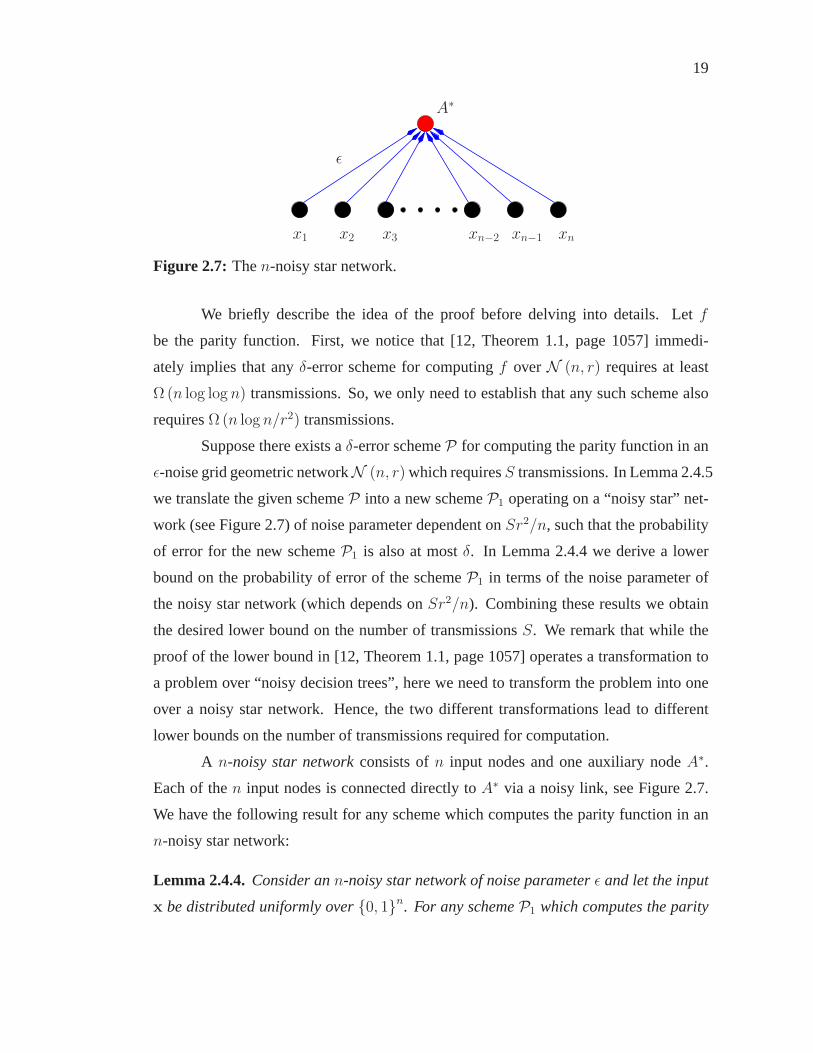
We briefly describe the idea of the proof before delving into details. Letf

be the parity function. First, we notice that [12, Theorem 1.1, page 1057] immedi-

ately implies that anyδ-error scheme for computingf overN (n, r) requires at least

Ω (n log log n) transmissions. So, we only need to establish that any such scheme also

requiresΩ (n log n/r2) transmissions.

Suppose there exists aδ-error schemeP for computing the parity function in an

ǫ-noise grid geometric networkN (n, r) which requiresS transmissions. In Lemma 2.4.5

we translate the given schemeP into a new schemeP1 operating on a “noisy star” net-

work (see Figure 2.7) of noise parameter dependent onSr2/n, such that the probability

of error for the new schemeP1 is also at mostδ. In Lemma 2.4.4 we derive a lower

bound on the probability of error of the schemeP1 in terms of the noise parameter of

the noisy star network (which depends onSr2/n). Combining these results we obtain

the desired lower bound on the number of transmissionsS. We remark that while the

proof of the lower bound in [12, Theorem 1.1, page 1057] operates a transformation to

a problem over “noisy decision trees”, here we need to transform the problem into one

over a noisy star network. Hence, the two different transformations lead to different

lower bounds on the number of transmissions required for computation.

A n-noisy star networkconsists ofn input nodes and one auxiliary nodeA∗.

Each of then input nodes is connected directly toA∗ via a noisy link, see Figure 2.7.

We have the following result for any scheme which computes the parity function in an

n-noisy star network:

Lemma 2.4.4.Consider ann-noisy star network of noise parameterǫ and let the input

x be distributed uniformly over0, 1n. For any schemeP1 which computes the parity

20

function (onn bits) in the network and in which each input node transmits its input bit

only once, the probability of error is at least(1− (1− 2ǫ)n) /2.

Proof. See Appendix 2.2.1.

We have the following lemma relating the original networkN (n, r) and a noisy

star network.

Lemma 2.4.5.Letα ∈ (0, 1). If there is aδ-error schemeP for computing the parity

function (onn input bits) inN (n, r) withS transmissions, then there is aδ-error scheme

P1 for computing the parity function (onαn input bits) in anαn-noisy star network with

noise parameterǫO(Sr2/n), with each input node transmitting its input bit only once.

Proof. See in Appendix 2.2.2.

We are now ready to complete the proof of Theorem 2.4.3.

Proof (of Theorem 2.4.3).Let α ∈ (0, 1). If there is aδ-error scheme for computing

the parity function inN (n, r) which requiresS transmissions, then by combining the

Lemmas 2.4.5 and 2.4.4, the following inequalities must hold:

δ ≥1−

(1− 2ǫO(Sr2/n)

)αn

2,

=⇒(1− 2ǫO(Sr2/n)

)αn

≥ 1− 2δ

=⇒(

2−2ǫO(Sr2/n)

)αn (a)

≥ 1− 2δ

=⇒ S ≥ Ω

(n (log n− log log (1/(1− 2δ)))

r2 log(1/ǫ)

)(2.1)

where(a) follows since2−x ≥ 1 − x for everyx > 0. Thus we have that anyδ-error

scheme for computing the parity function in anǫ-noise networkN (n, r) requires at

leastΩ (n log n/r2) transmissions.

We now consider the lower bound on the number of time slots. Since the mes-

sage of the farthest node requires at leastΩ (√n/r) time slots to reachρ, we have the

corresponding lower bound on the duration of anyδ-error scheme. The lower bound

of Ω (r2 log log n) time slots follows from the same argument as in the proof of Theo-

rem 2.4.1.

21

r/√

8

Θ(√

log n/ log log n)

A cell in N (n, r)

Sub-cell

Figure 2.8: Each cell in the networkN (n, r) is divided into sub-cells of side

Θ(√

log n/ log log n)

. Each sub-cell has a “head”, denoted by a yellow node. The

sum of input messages from each sub-cell is obtained at its head node, depicted by thesolid (blue) lines. These partial sums are then aggregated at the cell-center. The latterstep is represented by the dashed (magenta) lines.

We now present an efficient scheme for computing any symmetric function in a

noisy broadcast network which matches the above lower bounds.

Theorem 2.4.6.Letf be any symmetric function. Letδ ∈ (0, 1/2), let ǫ ∈ (0, 1/2), and

let r ∈ [1,√

2n]. There exists aδ-error scheme for computingf over anǫ-noise grid

geometric networkN (n, r) which requires at most

maxO (√n/r) , O (r2 log log n) time slots andmaxO (n log n/r2) , O (n log log n)

transmissions.

Proof. We present a scheme which can compute the arithmetic sum of the input bits

overN (n, r). Note that this suffices to prove the result sincef is symmetric and thus

its value only depends on the arithmetic sum of the input bits.

Consider the usual partition of the networkN (n, r) into cells of sizec× c with

c = r/√

8. For each cell, we pick one node arbitrarily and call it the “cell-center”. As

22

before, cells are scheduled to prevent interference between simultaneous transmissions

according to Figure 2.5. The scheme works in three phases.

First phase: The objective of the first phase is to ensure that each cell-center

computes the arithmetic sum of the input messages from the corresponding cell. De-

pending on the connection radiusr, this is achieved using two different strategies.

• r ≤√

log n/ log log n: In Appendix 2.3, we describe a scheme which can

compute the partial sums at all cell-centers with probability at least1 − O(1/n) and

requiresO (n/r2 × log n) total transmissions andO (log n) time slots.

• r >√

log n/ log log n: In this case, we first divide each cell into smaller

sub-cells withΘ (log n/ log log n) nodes each, see Figure 2.8. Each sub-cell has an

arbitrarily chosen “head” node. In each sub-cell, we use theIntra-cell schemefrom [10,

Section III] to compute the sum of the input bits from the sub-cell at the corresponding

head node. This requiresO (log log n) transmissions from each node in the sub-cell.

Since there areO (r2) nodes in each cell and only one node in a cell can transmit in

a time slot, this step requiresO (r2 log log n) time slots and a total ofO (n log log n)

transmissions in the network. The probability that the computation fails in at least one

sub-cell is bounded byO(1/n).

Next, each head node encodes the sum of the input bits from itssub-cell into a

codeword of lengthO (log n) and transmits it to the corresponding cell-center. This step

requires a total ofO (n log log n) transmissions in the network andO (r2 log log n) time

slots and can be performed also with probability of error at mostO(1/n).

The received values are aggregated so that at the end of the first phase, all cell-

centers know the sum of their input bits in their cell with probability at least1−O(1/n).

The phase requiresO (n log log n) transmissions in the network andO (r2 log log n)

time slots to complete.

Second phase:In this phase, the partial sums stored at the cell-centers are aggre-

gated along a tree (see for example, Figure 2.6) so that the sink nodeρ can compute the

sum of all the input bits in the network. We have the followingtwo cases, depending on

the connection radiusr.

• r ≥ (√n log n)

1/3: For this regime, our aggregation scheme is similar to

the Inter-cell schemein [10, Section III]. Each cell-center encodes its message into a

23

codeword of lengthΘ (log n). Each leaf node in the aggregation tree sends its codeword

to the parent node which decodes the message, sums it with itsown message and then re-

encodes it into a codeword of lengthΘ (log n). The process continues till the sink node

ρ receives the sum of all the input bits in the network. From Theorem 2.2.3, this phase

carries a probability of error at mostO(1/n). It requiresO (n log n/r2) transmissions

in the network andO (√n/r × log n) time slots.

• r ≤ (√n log n)

1/3: In this regime, the above simple aggregation scheme

does not match the lower bound for the latency in Theorem 2.4.3. A more sophisticated

aggregation scheme is presented in [11, Section V], which uses ideas from [16] to effi-

ciently simulate a scheme for noiseless networks in noisy networks. The phase carries

a probability of error at mostO(1/n). It requiresO (n log n/r2) transmissions in the

network andO (√n/r) time slots.

Combining the two phases, the above scheme can compute any symmetric func-

tion with probability of error at mostO(1/n). Thus forn large enough, we have aδ-error

scheme for computing any symmetric function in the networkN (n, r). It requires at

mostmaxO (√n/r) , O (r2 log log n) time slots and

maxO (n log n/r2) , O (n log log n) transmissions.

2.5 General Network Topologies

In the previous sections, we focused on grid geometric networks for their suitable

regularity properties and for ease of exposition. The extension to random geometric net-

works in the continuum plane whenr = Ω(√

log n)

is immediate, and we focus here on

extensions to more general topologies. First, we discuss extensions of our schemes for

computing symmetric functions and then present a generalized lower bound on the num-

ber of transmissions required to compute symmetric functions in arbitrary connected

networks.

2.5.1 Computing symmetric functions in noiseless networks

One of the key components for efficiently computing symmetric functions in

noiseless networks in Theorem 2.3.4 was the hierarchical scheme proposed for comput-

24

ing the arithmetic sum function in the grid geometric network N (n, 1). The main idea

behind the scheme was to consider successively coarser partitions of the network and at

any given level aggregate the partial sum of the input messages in each individual cell of

the partition using results from the finer partition in the previous level of the hierarchy.

Using this idea we extend the hierarchical scheme to any connected noiseless network

N and derive an upper bound on the number of transmissions required for the scheme.

Let each node in the network start with an input bit and denotethe set of nodes byV.

The scheme is defined by the following parameters:

• The number of levelsh.

• For each leveli, a partitionΠi = P 1i , P

2i , . . . , P

sii of the set of nodes in the

networkV into si disjoint cells such that eachP ji = ∪k∈T j

iP k

i−1 whereT ji ⊆

1, 2, . . . , si−1, i.e., each cell is composed of one or more cells from the next

lower level in the hierarchy. See Figure 2.9 for an illustration. Here,Π0 =

i : i ∈ V andΠh = V.

• For each cellP ji , a designated cell-centercji ∈ P j

i . Let c1h be the designated sink

nodev∗.

• For each cellP ji , letSj

i denote a Steiner tree with the minimum number of edges

which connects the corresponding cell-center with all the cell-centers of its com-

ponent cellsP ki−1, i.e., the set of nodes∪k∈T j

icki−1 ∪ cji . Let lji denote the number

of edges inSji .

Using the above definitions, the hierarchical scheme from Theorem 2.3.4 can now be

easily extended to general network topologies. We start with the first level in the hier-

archy and then proceed recursively. At any given level, we compute the partial sums

of the input messages in each individual cell of the partition at the corresponding cell-

centers by aggregating the results from the previous level along the minimum Steiner

tree. It is easy to verify that after the final level in the scheme, the sink nodev∗ pos-

sesses the arithmetic sum of all the input messages in the networkN . The total number

25

P 1t+1

P 1tP 2

t

P 3t P 4

t

c1t+1

c1tc2t

c3tc4t

Figure 2.9: Cell P 1t+1 is composed ofP k

t 4k=1 smaller cells from the previous level inthe hierarchy. Each of the cell-centersckt (denoted by the green nodes) holds the sum ofthe input bits in the corresponding cellP k

t . These partial sums are aggregated along theminimum Steiner treeS1

t+1 (denoted by the brown bold lines) so that the cell-centerc1t+1

(denoted by the blue node) can compute the sum of all the inputbits inP 1t+1.

of transmissions made by the scheme is at most

h−1∑

t=0

st+1∑

j=1

ljt+1 · log(∣∣P j

t+1

∣∣) .

Thus, we have a scheme for computing the arithmetic sum function in any arbitrary

connected network. In the proof of Theorem 2.3.4, the above bound is evaluated for the

grid geometric networkN (n, 1) with h = log√n, st = n/22t, ljt ≤ 4 ·2t−1,

∣∣P jt

∣∣ = 22t,

and is shown to beO(n).

2.5.2 Computing symmetric functions in noisy networks

We generalize the scheme in Theorem 2.4.6 for computing symmetric functions

in a noisy grid geometric networkN (n, r) to a more general class of network topolo-

gies and derive a corresponding upper bound on the number of transmissions required.

The original scheme consists of two phases: an intra-cell phase where the network is

26

partitioned into smaller cells, each of which is a clique, and partial sums are computed

in each individual cell; and an inter-cell phase where the partial sums in cells are aggre-

gated to compute the arithmetic sum of all input messages at the sink node. We extend

the above idea to more general topologies. First, for anyz ≥ 1, consider the following

definition:

Clique-cover property C(z): a networkN of n nodes is said to satisfy the

clique-cover propertyC(z) if the set of nodesV is covered by at most⌊n/z⌋ cliques,

each of size at mostlog n/ log log n.

For example, a grid geometric networkN (n, r) with r = O(√

log n/ log log n)

satisfiesC(z) for z = O(r2). On the other hand, a tree network satisfiesC(z) only for

z ≤ 2. Note that any connected network satisfies propertyC(1). By regarding each dis-

joint clique in the network as a cell, we can easily extend theanalysis in Theorem 2.4.6

to get the following result, whose proof is omitted.

Theorem 2.5.1.Let δ ∈(0, 1

2

), ǫ ∈

(0, 1

2

)andN be any connected network ofn

nodes withn ≥ 2/δ. For z ≥ 1, if N satisfiesC(z), then there exists aδ-error scheme

for computing any symmetric function overN which requires at mostO(n log n/z)

transmissions.

2.5.3 A generalized lower bound for symmetric functions

The proof techniques that we use to obtain lower bounds are also applicable to

more general network topologies. Recall thatN(i) denotes the set of neighbors for any

nodei. For any network, define the average degree as

d(n) =

∑

i∈V|N(i)|

n.

A slight modification to the proof of Theorem 2.4.3 leads to the following result:

Theorem 2.5.2.Let δ ∈(0, 1

2

)and let ǫ ∈

(0, 1

2

). There exists a symmetric target

functionf such that anyδ-error scheme for computingf over any connected network of

n nodes with average degreed(n), requires at leastΩ(

n log nd(n)

)transmissions.

27

Proof. Let f be the parity function. The only difficulty in adapting the proof of Theo-

rem 2.4.3 arises from the node degree not being necessarily the same for all the nodes.

We circumvent this problem as follows: in addition to decomposing the network into

the set of source nodesσ and auxiliary nodesA, such that|σ| = αn for α ∈ (0, 1), as

in the proof of Lemma 2.4.5 (see Appendix 2.2.2); we also let every source node with

degree more than2d(n)α

be an auxiliary node. There can be at mostαn2

of such nodes

in the network since the average degree isd(n). Thus, we obtain an(

αn2, (1− α

2)n)

decomposition of the network such that each source node has degree at most2d(n)α

. The

rest of the proof then follows in the same way.

As an application of the above result, we have the following lower bound for

ring or tree networks.

Corollary 2.5.3. Let f be the parity function, letδ ∈(0, 1

2

), and letǫ ∈

(0, 1

2

). Any

δ-error scheme for computingf over any ring or tree network ofn nodes requires at

leastΩ (n log n) transmissions.

The above result answers an open question, posed originallyby El Gamal [6].

2.6 Conclusion

We conclude with some observations and directions for future work.

2.6.1 Target functions

We considered all symmetric functions as a single class and presented a worst-

case characterization (up to a constant) of the number of transmissions and time slots

required for computing this class of functions. A natural question to ask is whether it

is possible to obtain better performance if one restricts toa particular sub-class of sym-

metric functions. For example, two sub-classes of symmetric functions are considered

in [3]: type-sensitiveand type-threshold. Since the parity function is a type-sensitive

function, the characterization for noiseless networks in Theorems 2.3.3 and 2.3.4, as

well as noisy broadcast networks in Theorems 2.4.3 and 2.4.6also holds for the re-

stricted sub-class of type-sensitive functions. A similargeneral characterization is not

28

possible for type-threshold functions since the trivial function (f(x) = 0 for all x) is also

in this class and it requires no transmissions and time slotsto compute. The following

result, whose proof follows similar lines as the results in previous sections and is omit-

ted, characterizes the number of transmissions and the number of time slots required

for computing the maximum function, which is an example type-threshold function.

This can be compared with the corresponding results for the whole class of symmetric

functions in Theorems 2.4.3 and 2.4.6.

Theorem 2.6.1.Let f be the maximum function. Letδ ∈ (0, 1/2), ǫ ∈ (0, 1/2), and

r ∈ [1,√

2n]. Anyδ-error scheme for computingf over anǫ-noise networkN (n, r)

requires at leastmaxΩ (√n/r) ,Ω (r2) time slots andmaxΩ (n log n/r2) ,Ω (n)

transmissions. Further, there exists aδ-error scheme for computingf which requires

at mostmaxO (√n/r) , O (r2) time slots andmaxO (n log n/r2) , O (n) transmis-

sions.

2.6.2 On the role ofǫ and δ

Throughout the paper, the channel error parameterǫ and the thresholdδ on the

probability of error are taken to be given constants. It is also interesting to study how the

cost of computation depends on these parameters. The careful reader might have noticed

that our proposed schemes work also when only an upper bound on the channel error

parameterǫ is considered, and always achieve a probability of errorδ that is either zero

or tends to zero asn→∞. It is also clear that the cost of computation should decrease

with smaller values ofǫ and increase with smaller values ofδ. Indeed, from (2.1) in

the proof of Theorem 2.4.3 we see that the lower bound on the number of transmissions

required for computing the parity function depends onǫ as1/(− log ǫ). On the other

hand, from the proof of Theorem 2.4.6 the upper bound on the number of transmissions

required to compute any symmetric function depends onǫ as1/ (− log(ǫ(1− ǫ))). The

two expressions are close for small values ofǫ.

29

2.6.3 Network models

We assumed that each node in the network has a single bit value. Our results

can be immediately adapted to obtain upper bounds on the latency and number of trans-

missions required for the more general scenario where each nodei observes a block of

input messagesx1i , x

2i , . . . , x

ki with eachxj

i ∈ 0, 1, . . . , q, q ≥ 2. However, finding

matching lower bounds seems to be more challenging.

Appendix

2.1 Computing the arithmetic sum overN (n, 1)

m

m/2

Ami

Am/2i1

Am/2i2

Am/2i3

Am/2i4

u(Ami ), u

(Am/2i3

)u(Am/2i4

)

Figure 2.10: Ami is a square cell of sizem × m. This figure illustrates some notation

with regards toAmi .

Consider a noiseless networkN (n, 1) where each nodei has an input message

xi ∈ 0, 1, . . . , q − 1. We present a scheme which can compute the arithmetic sum

of the input messages over the network inO (√n+ log q · log n) time slots and using

O (n+ log q) transmissions. We briefly present the main idea of the schemebefore

30

√n

2k+1

ρ

A2k+1

1A2k+1

2

u(A2k+1

2 ) u(A2k+1

1 )

Figure 2.11: This figure illustrates the partition of the networkN (n, 1) into smaller

cellsA2k+1

i

n

22(k+1)

i=1, each of size2k+1 × 2k+1.

delving into details. Our scheme divides the network into small cells and computes the

sum of the input messages in each individual cell at designated cell-centers. We then

proceed recursively and in each iteration we double the sizeof the cells into which the

network is partitioned and compute the partial sums by aggregating the computed values

from the previous round. This process finally yields the arithmetic sum of all the input

messages in the network.

Before we describe the scheme, we define some notation. Consider anm ×msquare cell in the network, see Figure 2.10. Denote this cellbyAm

i and the node in the

lower-left corner ofAmi by u (Am

i ). For anym which is a power of2, m ≥ 2, Ami can

be divided into4 smaller cells, each of sizem/2×m/2, see Figure 2.10. Denote these

cells byA

m/2ij

4

j=1.

Without loss of generality, letn be a power of4. The scheme has the following

steps :

1. Letk = 0.

2. Consider the partition of the network into cellsA2k+1

i

n

22(k+1)

i=1each of size2k+1×

31

A2k+1

i

2k

2k+1

A2ki1

A2ki2

A2ki3

A2ki4

u(A2k

i1

)u(A2k

i2

)

u(A2k+1

i

), u(A2k

i3

)u(A2k

i4

)

Figure 2.12: Step2 of the scheme for computing the sum of input messages. The net-work is divided into smaller cells, each of size2k+1 × 2k+1. For any such cellA2k+1

i ,

j ∈ 1, 2, 3, 4, each corner nodeu(A2k

ij

)has the sum of the input messages corre-

sponding to the nodes in the cellA2k

ij. Then the sum of the input messages corresponding

to the cellA2k+1

i is aggregated atu(A2k+1

i

), along the tree shown in the figure.

2k+1, see Figure 2.11. Note that each cellA2k+1

i consists of exactly four cellsA2k

i1, . . . , A2k

i4

, see Figure 2.12. Each corner nodeu

(A2k

ij

), j = 1, 2, 3, 4 pos-

sesses the sum of the input messages corresponding to the nodes in the cellA2k

ij.

The partial sums stored atu(A2k

ij

), j = 1, 2, 3, 4 are aggregated at the node

u(A2k+1

i

), along the tree shown in Figure 2.12. Each node in the tree makes

at mostlog(22(k+1)q

)transmissions.

At the end of this step, each corner nodeu(A2k+1

i

)has the sum of the input mes-

sages corresponding to the nodes in the cellA2k+1

i . By pipelining the transmissions

along the tree, this step takes at most

2(2k + log

(22(k+1)q

))time slots.

32

The total number of transmissions in the network for this step is at most

n

22(k+1)· 4 · 2k · log

(22(k+1)q

)=

4n

2k+1(k + 1 + log q) .

3. Letk ← k + 1. If 2k+1 ≤ √n, return to step2, else terminate.

Note that at the end of the process, the nodeρ can compute the sum of the input messages

for any inputx ∈ 0, 1, . . . , q − 1n. The total number of steps in the scheme islog√n.

The number of time slots that the scheme takes is at most

log√

n−1∑

k=0

2(2k + log

(22(k+1)q

))

≤ O(log q · log n+

√n).

The total number of transmissions made by the scheme is at most

log√

n−1∑

k=0

4n(k + 1 + log q)

2k+1

≤ O (n+ log q) .

2.2 Completion of the proof of Theorem 2.4.3

2.2.1 Proof of Lemma 2.4.4

For everyi ∈ 1, 2, . . . , n, let yi be the noisy copy ofxi that the auxiliary node

A∗ receives. Denote the received vector byy. The objective ofA∗ is to compute the

parity of the input bitsx1, x2, . . . , xn. Thus, the target functionf is defined as

f (x) = x1 ⊕ x2 ⊕ . . .⊕ xn.

Since the inputx is uniformly distributed, we havePr (f(x) = 0) = Pr (f(x) = 1) =

1/2. In the following, we first show that Maximum Likelihood estimation is equivalent

to using the parity of the received bitsy1, y2, . . . , yn i.e. f(y) as an estimate forf(x), and

then compute the corresponding probability of error. From the definition of Maximum

33

Likelihood estimation, we have

f =

1 if Pr (y|f(x) = 1) > Pr (y|f(x) = 0)

0 otherwise.

Next,

Pr (y|f(x) = 1) =∑

x∈0,1n

s.tf(x)=1

Pr(x|f(x = 1)) · Pr (y|x)

(a)= κ

∑

x∈0,1n

s.tf(x)=1

Pr (y1|x1) Pr (y2|x2) . . .Pr (yn|xn)

whereκ = 2−(n−1) and(a) follows sincex is uniformly distributed over0, 1n and

from the independence of the channels between the sources and the auxiliary node.

Similarly,

Pr (y|f(x) = 0) = κ∑

x∈0,1n

s.tf(x)=0

Pr (y1|x1) Pr (y2|x2) . . .Pr (yn|xn) .

Putting things together, we have

Pr (y|f(x) = 0)− Pr (y|f(x) = 1) = κ

∑

x∈0,1n

s.tf(x)=0

n∏

i=1

Pr (yi|xi)−∑

x∈0,1n

s.tf(x)=1

n∏

i=1

Pr (yi|xi)

(a)= κ

n∏

i=1

(Pr(yi|xi = 0)− Pr(yi|xi = 1))

= κ (−1)n1(y) (1− 2ǫ)n , (2.2)

wheren1(y) is the number of components iny with value1. The above equality(a) can

be verfied by noting that the product in(a) produces a sum of2n monomials and that the

sign of each monomial is positive if the number of terms of themonomial conditioned

34

onxi = 1 is even, and negative otherwise. From (2.2), we now have

Pr (y|f(x) = 0)− Pr (y|f(x) = 1)

> 0 if f(y) = 0

< 0 if f(y) = 1.

Thus, we have shown that Maximum Likelihood estimation is equivalent to usingf(y)

as an estimate forf(x). The corresponding probability of error is given by

PrML (Error) = Pr (f(y) 6= f(x))

=

⌈n2⌉∑

j=1

Pr

(n∑

i=1

xi ⊕ yi = 2j − 1

)

=

⌈n2⌉∑

j=1

(n

2j − 1

)ǫ2j−1 (1− ǫ)n−2j+1

=1− (1− 2ǫ)n

2.

Hence, for any schemeP1 which computes the parity functionf in an n-noisy star

network, the probability of error is at least(1− (1− 2ǫ)n) /2.

2.2.2 Proof of Lemma 2.4.5

We borrow some notation from [8] and [12]. Consider the nodes in a network

and mark a subsetσ of them as input nodes and the restA as auxiliary nodes. Such a

decomposition of the network is called an(|σ| , |A|)-decomposition. An input value to

this network is an element of0, 1|σ|. Consider a schemeP on such a network which

computes a functionf of the input. The scheme is said to bem-bounded with respect to

an (|σ| , |A|)-decomposition if each node inσ makes at mostm transmissions. Recall

from Section 2.2 that for any scheme in our model, the number of transmissions that

any node makes is fixed a priori and does not depend on a particular execution of the

scheme. Following [8] and [12] we define thesemi-noisy network, in which whenever it

is the turn of an input node to transmit, it sends its input bitwhose independentǫ-noisy

copies are received by its neighbors, while the transmission made by auxiliary nodes are

not subject to any noise.

35

The proof now proceeds by combining three lemmas. Suppose there exists aδ-

error schemeP for computing the parity function in anǫ-noise networkN (n, r) which

requiresS transmissions. We first show in Lemma 2.2.1 that this impliesthe existence of

a suitable decomposition of the network and aδ-error,O (S/n)-bounded schemePd for

computing the parity function in this decomposed network. Lemma 2.2.2 translates the

schemePd into a schemePs for computing in a semi-noisy network and Lemma 2.2.3

translatesPs into a schemeP1 for computing in a noisy star network, while ensuring

that the probability of error does not increase at any intermediate step. The proof is

completed using the fact that the probability of error for original schemeP is at mostδ.

Let α ∈ (0, 1). We have the following lemma.

Lemma 2.2.1.If there is aδ-error schemeP for computing the parity function (onn in-

put bits) inN (n, r) withS transmissions, then there is an(αn, (1− α)n)-decomposition

ofN (n, r) and aδ-error, O (S/n)-bounded schemePd for computing the parity func-

tion (onαn bits) in this decomposed network.

Proof. If all nodes in the network makeO (S/n) transmissions, then the lemma fol-

lows trivially. Otherwise, we decompose the network into the set of input nodesσ and

auxiliary nodesA as follows. Consider the set of nodes which make more thanSn(1−α)

transmissions each during the execution of the schemeP. SinceP requiresS transmis-

sions, there can be at most(1 − α)n of such nodes. We let these nodes be auxiliary

nodes and let their input be0. Thus, we have an(αn, (1− α)n)-decomposition of the

networkN (n, r). The scheme now reduces to computing the parity (onαn bits) over

this decomposed network. By construction, each input node makes at most Sn(1−α)

trans-

missions and hence the scheme isO (S/n)-bounded.

The following lemma is stated without proof, as it follows immediately from [8,

Section 6, page 1833], or [12, Lemma 5.1, page 1064].

Lemma 2.2.2. (FROM NOISY TO SEMI-NOISY)For any functionf : 0, 1αn → 0, 1and anyδ-error, O (S/n)-bounded schemePd for computingf in an (αn, (1− α)n)-

decomposition ofN (n, r), there exists an(αn, n)-decomposed semi-noisy network of

(1 + α)n nodes such that each input node has at mostO (r2) neighbors and aδ-error,

O (S/n)-bounded schemePs for computingf in the semi-noisy network.

36

We now present the final lemma needed to complete the proof.

Lemma 2.2.3. (FROM SEMI-NOISY TO NOISY STAR)For any functionf : 0, 1αn →0, 1 and anyδ-error, O (S/n)-bounded schemePs for computingf in an (αn, n)-

decomposed semi-noisy network where each input node has at most O (r2) neighbors,

there exists aδ-error schemeP1 for computingf in anαn-noisy star network with noise

parameterǫO(Sr2/n), with each input node transmitting its input bit only once.

Proof. In a semi-noisy network, when it is the turn of an input node totransmit during

the execution ofPs, it transmits its input bit. Since the bits sent by the input nodes do

not depend on bits that these nodes receive during the execution of the scheme, we can

assume that the input nodes make their transmissions at the beginning of the scheme

an appropriate number of times, and after that only the auxiliary nodes communicate

without any noise. Further, since any input node in the(αn, n)-decomposed network

has at mostO (r2) neighbors, at mostO (r2) auxiliary nodes receive independentǫ-

noisy copies of each such input bit. SincePs is anO (S/n)-bounded scheme, each

input node makes at mostO (S/n) transmissions and hence the auxiliary nodes receive

a total of at mostO (Sr2/n) independentǫ-noisy copies of each input bit.

Next, we use the schemePs to construct a schemeP1 for computingf in an

αn-noisy star network of noise parameterǫO(Sr2/n) with each input node transmitting its

input bit only once. Lemma 2.2.4 shows that upon receiving anǫO(Sr2/n)-noisy copy for

every input bit, the auxiliary nodeA∗ in the noisy star network can generateO (Sr2/n)

independentǫ-noisy copies for each input bit. Then onwards, the auxiliary nodeA∗ can

simulate the schemePs. This is true since forPs only the auxiliary nodes operate after

the initial transmissions by the input nodes, and their transmissions are not subject to

any noise.

Lemma 2.2.4. [8, Lemma 36, page 1834] Lett ∈ N, ǫ ∈ (0, 1/2), andγ = ǫt. There

is a randomized algorithm that takes as input a single bitb and outputs a sequence oft

bits such that if the input is aγ-noisy copy of0 (respectively of1), then the output is a

sequence of independentǫ-noisy copies of0 (respectively of1).

37

2.3 Scheme for computing partial sums at cell-centers

We describe an adaptation of the scheme in [10, Section III],which requires at

mostO(

n log nr2

)transmissions andO (log n) time slots. The scheme in [10, Section III]

is described forr >√

log n and while the same ideas work forr ≤√

log n/ log log n,

the parameters need to be chosen carefully so that the schemecan compute efficiently

in the new regime.

Recall that the network is partitioned into cells of sizec × c wherec = r/√

8.

Consider any cellA1 in the network and denote its cell-center byv1. The scheme has

the following steps:

1. Every node inA1 takes a turn to transmit its input bitxi, 6λ

(log nc2

)times, where

λ = − ln (4ǫ(1− ǫ)). Thus, every node inA1 receives8λ

(log nc2

)independent noisy

copies of the entire input. This step requiresn · 8λ

(log nc2

)transmissions and8 log n

λ

time slots.

2. Each node inA1 forms an estimate for the input bits of the other nodes inA1 by

taking themajority of the noisy bits that it received from each of them. It is easy

to compute the probability that a node has a wrong estimate for any given input bit

to be at mostc2 · e− 4 log n

c2 , see for example Gallager’s book [15, page 125]. Each

node then computes the arithmetic sum of all the decoded bitsand thus has an

estimate of the sum of all the input bits in the cellA1.

3. Each node inA1 transmits its estimate to the cell-centerv1 using a codeword of

lengthk log nc2

such thatk is a constant and the cell-center decodes the message with

probability of error at moste−4 log n

c2 . The existence of such a code is guaranteed by

Theorem 2.2.3 and from the fact that the size of the estimate in bitslog(c2 + 1) ≤log n/c2, sincec2 = r2

8≤ log n

8 log log n. At the end of this step,v1 hasc2 independent

estimates for the sum of the input bits corresponding to the nodes inA1. The total

number of transmissions for this step is at mostn · k log nc2

and it requires at most

k log n time slots.

4. The cell-centerv1 takes themodeof thesec2 values to make the final estimate for

the sum of the input bits inA1.

38

We can now bound the probability of error for the scheme as follows.

Pr(Error) ≤(4(c2e−

4 log n

c2 + e−4 log n

c2

)(1− (c2e−

4 log n

c2 + e−4 log n

c2 )))c2

(a)

≤(4 · 9c2e− 4 log n

c2

)c2

(b)

≤ 1

n2, for n large enough

where(a) follows since8c2 = r2 ≥ 1; and(b) follows sincec2 log c2 ≤ log n. Thus,

every cell-centervi can compute the sum of the input bits corresponding to the nodes

in Ai with probability of error at most1n2 . The total probability of error is then at most

nc2· 1

n2 ≤ 1n. The total number of transmissions in the network for this scheme is at most

(8λ

+ k)· n log n

c2, i.e. O

(n log n

r2

)and it takes at most

(8λ

+ k)· log n, i.e.,O (log n) time

slots.

Chapter 2, in part, has been submitted for publication of the material. The dis-

sertation author was the primary investigator and author ofthis paper.

Chapter 3

Function computation over linear

channels

We consider multiple sources communicating over a network to a common sink.

We assume that the network operation is fixed, and its end result is to convey a fixed

unkown linear transformation of the source data to the sink.We design communication

protocols that can perform computation without modifying the network operation, by

appropriately selecting the codebook that the sources employ to map their measurements

to the data they send over the network. The model studied in this chapter is motivated

by practical considerations: since implementing networking protocols is hard, there is a

strong incentive to reuse the same network protocol to compute different functions.

39

40

3.1 Introduction

In sensor networks, the need for energy efficiency has stimulated research efforts

towards in-network aggregation and function computation,see for example [3, 17, 18].

Recent work [19,20] has also pointed out the need to havesimplecoding schemes, since

“systems are hard to develop and debug”. They advocate a solution where most nodes

in the network perform the same operations regardless of thefunction to be computed,

and the onus of guaranteeing successful computation is on a few special nodes that are

allowed to vary their operation.

Motivated by the above considerations, we consider the problem of computing

functions in a network where multiple sources are connectedto a single sink via relays.

The sources may have several different possible codebooks,and can select which one

to employ depending on the function to be computed. Given a certain target function,

each source transmits a codeword corresponding to its observed message. The relay

nodes, however, perform the same linear operations, for example randomized network

coding (which is a practical and efficient way of transmitting data in a network [21])

irrespective of the target function, i.e., the vectors inserted by the sources are randomly

combined and forwarded towards the sink, using linear coefficients that are unknown to

both the sources and the sink. The sink then proceeds to evaluate the target function of

the source messages.

Following [22–24], we use subspace coding for computing functions in our net-

work model. Given a target function, we assume that each source uses a codebook

consisting of subspaces. Each source message is mapped to a subspace in the codebook.

When a source generates a message, it injects the basis vectors of the corresponding

subspace into the network. The network operation is abstracted by assuming that the

sink collects enough linear combinations of these vectors to learn the joint span of the

injected subspaces. Given this information, the sink then attempts to compute the target

function of the source messages. Our objective is to design codebooks which minimize

the number of symbols each source needs to transmit, while guaranteeing successful

function computation by the sink.

Thus, we envision a network architecture where intermediate network nodes al-

ways perform the same operations for information transfer,which leads to a simple

41

implementation. At the same time, the sink has the flexibility to utilize the network to

learn different functions of the source data by informing the source nodes to employ the

corresponding codebooks. Here we focus on non-coherent communication where we

have no knowledge about the network transformation; in [25]we look at the case where

this transformation is fixed and known.

We note that a scheme which optimizes the intermediate node operations accord-

ing to the function to be computed might need fewer transmissions. However, it would

be more complex to implement, would require topology knowledge, and might be sen-

sitive to the employed communication protocol. In contrast, our approach is transparent

both to the topology and the employed communication protocol: the only requirement

we impose is that we gather sufficient linear independent combinations. As a result, our

protocol would be very well suited to dynamically changing topologies, and could be

applied without change on top of very different communication protocols.

The chapter is organized as follows. Section 3.2 presents the problem formu-

lation. In Section 3.3, we present various lower bounds on the number of symbols

each source needs to transmit to evaluate an arbitrary function. In Section 3.4, we dis-

cuss various example target functions. In particular, we provide lower bounds as well

as near-optimal coding schemes for theidentity, T -threshold, maximumandK-largest

valuesfunctions. Finally, in Section 3.3, we present a constructive scheme to evaluate

arbitrary functions.

3.2 Problem Formulation and Notation

We consider a set ofs sourcesσ1, σ2, . . . , σs connected to a sinkρ via a network

N . Each sourceσi is either inactive or observes a messagexi ∈ A, whereA is a finite

alphabet. For ease of notation, when a sourceσi is inactive we will setxi = φ. The sink

needs to compute atarget functionf of the source messages, wheref is of the form

f : (A ∪ φ)s −→ B.

Some example target functions are defined below.

42

x1∈A∪φ

x2

πx11 ⊆ F

lq

xs

NetworkN

Sinkρ

f (x1, . . . , xs)

s∑

i=1

πxii

Figure 3.1: Description of the network operation

Definition 3.2.1.

• The identitytarget function hasB = (A ∪ φ)s and is defined by

f (x1, . . . , xs) = (x1, . . . , xs) .

• For m ≥ 1, the arithmetic sumtarget function hasA = 1, . . . ,m, B =

0, 1, . . . ,ms, and is defined by

f (x1, . . . , xs) = x1 + x2 + · · ·+ xs

where ‘+’ denotes ordinary integer summation. For anya ∈ A ∪ φ, we set

a+ φ = a.

• LetA be an ordered set. Themaximumtarget function hasB = A and is defined

by

f (x1, . . . , xs) = max x1, . . . , xs .

For anya ∈ A ∪ φ, we setmaxa, φ = a.

• Theparity target function hasA = B = 0, 1, and is defined by

f (x1, . . . , xs) = x1 ⊕ x2 ⊕ . . .⊕ xs

where⊕ denotesmod-2 addition. Again, for anya ∈ A∪ φ we seta⊕ φ = a.

43

• Themajority target function hasA = B = 0, 1, and is defined by

f (x1, . . . , xs) =

1 if |i : xi = 1| > |i : xi = 0|

0 otherwise.

We consider operation using subspace coding. We denote a subspace byπ and

the union of two subspacesπ1, π2 is defined asπ1 + π2 = x + y : x ∈ π1,y ∈ π2.The network operates as follows.

• At each source, every alphabet symbol is mapped to a subspace, which serves as

the corresponding codeword. Thus, each sourceσi has an associated codebook

Ci =πj

i

j∈A whereπj

i is ad-dimensional subspace1 of an l-dimensional vector

spaceFlq whered, l ≥ 1 are design parameters. When the sourceσi is active and

observes a messagexi ∈ A, it injects into the networkN a set ofd vectors from

Flq which span the subspaceπxi

i . When the source isσi inactive, it does not make

any transmissions and hence we setπφi = ∅.

• The sinkρ receives from the networkN a set of vectors fromFlq which span the

union of the input subspaces2 i.e.,ρ observes∑s

i=1 πxii .

• The sink uses the received information to compute the value of f (x1, x2, . . . , xs).

A (d, l) feasible code for computingf is a collection of codebooksC1, C2, . . . , Cssuch that eachπj

i in the codebooks is ad-dimensional subspace ofFlq and the sink can

compute the value off (x1, x2, . . . , xs) for any choice of input messagesx1, x2, . . . , xs

where eachxi ∈ A ∪ φ.For a(d, l) feasible code for computingf , each source transmits at mostd · l

symbols fromFq, and we thus consider the associated cost3 to bed · l. Our code design

seeks to achieve

Emin(f)=inf d · l : ∃ a (d, l) feasible code for computingf .1Although restricting our code design to subspaces of equal dimension may not always be optimal, it

significantly simplies the design, and is a standard approach in the literature [22,26].2In practice, networks operate in rounds. The duration of a round can be chosen large enough to ensure

that the sink receives enough linear independent combinations to span the union of the input subspaces.3In this work, the field sizeq is considered to be fixed and hence not included in the cost.

44

We begin by showing that for the purpose of minimizing the cost d · l, it suffices to

consider codes which use one-dimensional subspaces.

Theorem 3.2.2.Given any(d, l) feasible code for computing a target functionf , there

also exists a(1, d · l) feasible code for computingf .

Proof. Partition(A∪φ)s intoP1, P2, . . . , P|B| so that eachPi consists of all the input

vectors which result in the same function value. Then a necessary and sufficient condi-

tion for successful computation is that the sink should receive different union subspaces

for any two input vectorsx andy if they belong to distinct partitions.

Let πji ⊆ F

lq : i ∈ 1, . . . , s, j ∈ A denote the collection ofd-dimensional

subspaces associated with the given(d, l) feasible code for computingf . The above

necessary condition implies that these subspaces satisfy acollection of inequalities, each

of the forms∑

i=1

πaii 6=

s∑

i=1

πbii (3.1)

where eachai, bi ∈ A∪ φ. Now corresponding to eachd-dimensional subspaceπji in

the above code, construct a one-dimensional subspaceπji ⊆ F

d·lq by concatenating the

d basis vectors ofπji into a single vector. It can be verified that the collection ofone-

dimensional subspacesπji : i ∈ 1, . . . , s, j ∈ A constructed this way also satisfy

all the inequalities that the original code satisfied, i.e.,if (3.1) holds for someai, bi,then

s∑

i=1

πaii 6=

s∑

i=1

πbii . (3.2)

Since (3.1) holds, there exists at least one basis vector, say v1 ∈ πa11 , which is not in

∑si=1 π

bii . This immediately implies thatπa1

1 cannot be an element of∑s

i=1 πbii , which

proves (3.2).

Thus the collection of one-dimensional subspacesπji : i ∈ 1, . . . , s, j ∈ A

ensures that for any two input vectors in distinct partitions, the sink receives different

union subspaces. Since this is sufficient for function computation, we have shown that

we can construct a(1, d · l) feasible code from any(d, l) feasible code.

In the sequel, we will only consider codes which use one-dimensional subspaces.

We will denote the dimension of any subspaceπ by dim(π). Also, for any vectorx, the

45

j-th component will be denoted by(x)j. Consider a set of indicesI =(i1, i2, . . . , i|I|

)⊆

1, . . . , s. For anya =(a1, a2, . . . , a|I|

)∈ (A∪φ)|I| and any vectorx ∈ (A∪φ)s,

let x(I, a) = (x1, x2, . . . , xs) denote a vector which is obtained fromx by substituting

the components corresponding to the index setI with values from the vectora and

retaining all the other components. That is, for eachj ∈ 1, . . . , |I|, (x(I, a))ij= (a)j

and for eachk 6∈ I, (x(I, a))k = (x)k . We conclude this section with a lemma that is

often used in the subsequent sections.

Lemma 3.2.3. If there exist one-dimensional subspacesπ1, π2, . . . , πK ⊆ Flq and a

subspaceπ∗ ⊆ Flq such that

πi 6⊆ π∗ +∑

j<i

πj ∀ i ∈ 1, . . . , K (3.3)

thenl ≥ K.

Proof. (3.3) implies that the basis vectors for theK one-dimensional subspaces are

linearly independent. The result then follows.

3.3 Lower bounds

The number ofd-dimensional subspaces ofFlq for anyd ≤ l, l ≥ 1 is given by

the gaussian binomial coefficient

[l

d

]

q

=(ql − 1)(ql−1 − 1) · · · (ql−d+1 − 1)

(qd − 1)(qd−1 − 1) · · · (q − 1). (3.4)

We have the following upper bound on the number ofd-dimensional subspaces..

Lemma 3.3.1. The number ofd-dimensional subspaces ofFlq is at most4qd(l−d) [22,

Lemma 4].

Recall thatx(I, a) denotes a vector which is obtained fromx by substituting the

components corresponding to the index setI with values from the vectora and retaining

all the other components. Consider a target function with thefollowing property.

46

Function propertyP : There existsk ∈ 1, . . . , s andx ∈ (A∪φ)s such that

for anya, b ∈ A,

f(x(k, a)) 6= f(x(k, b)).

Examples: The identity function and arithmetic sum function satisfypropertyP.

We have the following simple lower bound for functions whichsatisfy property

P.

Lemma 3.3.2.For any target functionf which satisfies propertyP,

Emin(f) ≥ logq (|A| (q − 1)) + 1.

Proof. From the definition of propertyP, there existsk such that sourceσk must assign

a distinct one-dimensional subspace to eacha ∈ A. From (3.4), we have

ql − 1

q − 1≥ |A|

=⇒ l ≥ logq (|A| (q − 1)) + 1.

Consider a target function with the following property.

Function propertyQ(k) : There existsx ∈ (A ∪ φ)s and a collection ofk

distinct indicesi1, i2, . . . , ik such that for everyj ∈ 1, 2, . . . , k, we have(x)j 6= φ and

f (x(i1, . . . , ij−1, φ, . . . , φ)) 6= f (x(i1, . . . , ij−1, ij, φ, . . . , φ)) . (3.5)

Example 3.3.3.

• The identity function satisfies propertyQ(s) by choosing each(x)j equal to any

element of the alphabetA.

• The arithmetic sum function satisfies propertyQ(s) by choosing each(x)j equal

to some non-zero element of the alphabetA.

• The parity function satisfies propertyQ(s) by choosing each(x)j equal to1.

47

• The majority function satisfies propertyQ(s) by choosing(x)j equal to1 if j is

even and0 otherwise whens is even and vice-versa whens is odd.

Lemma 3.3.4.For any target functionf which satisfies propertyQ(k),

Emin(f) ≥ k.

Proof. Let

Πc =∑

t6∈i1,i2,...,ikπ

(x)t

t .

From (3.5), any feasible code for computingf should satisfy for everyj ∈ 1, 2, . . . , k

π(x)ij

ij+

k∑

m=j+1

π(x)imim

+ Πc 6=k∑

m=j+1

π(x)imim

+ Πc

=⇒ π(x)ij

ij6⊆

k∑

m=j+1

π(x)imim

+ Πc.

Then using Lemma 3.2.3 for the collection ofk one-dimensional subspacesπ(x)i1i1

, . . . , π(x)ikik

and the subspaceΠc, the result follows.

We borrow the following definition from [18].

Definition 3.3.5. For any target functionf : (A ∪ φ)s −→ B, any index setI ⊆1, 2, . . . , s, and anya,b ∈ (A∪φ)|I|, we writea ≡ b if for everyx ∈ (A∪φ)s,

we havef (x(I, a)) = f (x(I,b)).

It can be verified that≡ is an equivalence relation4 for everyf andI.

Definition 3.3.6. For everyf andI, let RI,f denote the total number of equivalence

classes induced by≡ and let

ΦI,f : (A ∪ φ)|I| −→ 1, 2, . . . , RI,f4Witsenhausen [27] represented this equivalence relation in terms of the independent sets of a char-

acteristic graph and his representation has been used in various problems related to function computa-tion [28, 29]. Although≡ is defined with respect to a particular index setI and a functionf , we do notmake this dependence explicit – the values ofI andf will be clear from the context.

48

be any function such thatΦI,f (a) = ΦI,f (b) iff a ≡ b.

That is,ΦI,f assigns a unique index to each equivalence class, and

RI,f =∣∣ΦI,f (a) : a ∈ (A ∪ φ)|I|

∣∣ .

The value ofRI,f is independent of the choice ofΦI,f .

Example 3.3.7.

• Let f be the identity target function. Then for everya,b ∈ (A ∪ φ)|I| we have

a ≡ b if and only if a = b. The number of distinct equivalence classes is

RI,f = (|A|+ 1)|I|.

• Let A = 1, . . . ,m for somem ≥ 1 and letf be the arithmetic sum target

function. Fora,b ∈ (A ∪ φ)|I|, we havea ≡ b if and only if

|I|∑

i=1

(a)i =

|I|∑

i=1

(b)i

and the number of such possible sums is

RI,f = m |I|+ 1.

Lemma 3.3.8.For any target functionf ,

Emin(f) ≥ maxI

max

√logq (RI,f )

3,logq(RI,f )

3 |I|

.

Proof. Consider anyI = i1, i2, . . . , i|I|. For anya,b ∈ (A∪φ)|I| such thata 6≡ b,

any feasible code should satisfy

∑

j∈1,...,|I|π

(a)j

ij6=

∑

j∈1,...,|I|π

(b)j

ij. (3.6)

49

Note that for anyI anda ∈ (A ∪ φ)|I|, dim(∑

j∈1,...,|I| π(a)j

ij

)≤ |I| since it is

composed of the union of at most|I| one-dimensional subspaces. Then from Defini-

tion 4.1.4 and (3.6), there exist at leastRI,f distinct subspaces, each with dimension at

most|I|. From Lemma 3.3.1, we have

4 ·minl,|I|∑

j=1

qj(l−j) ≥ RI,f . (3.7)

This implies that

4 ·l∑

j=1

qj(l−j) ≥ RI,f

=⇒4l · q( l2)

2

≥ RI,f

=⇒ logq(4l) +

(l

2

)2

≥ logq(RI,f ).

Sincelogq(4l) ≤ 2l2, we have

3l2 ≥ logq(RI,f )

=⇒ l ≥

√logq(RI,f )

3.

From (3.7), we also have

4 ·|I|∑

j=1

qj(l−j) ≥ RI,f

=⇒4 |I| · qd(l−d) ≥ RI,f with d = argmaxj∈1,|I|

qj(l−j)

=⇒ logq(4 |I|) + d(l − d)+ ≥ logq(RI,f ).

50

Sincelogq(4 |I|) ≤ 2 |I| andd ≤ |I|, we have

2 |I| l + |I| l ≥ logq(RI,f )

=⇒ l ≥ logq(RI,f )

3 |I| .

Example 3.3.9.

• For the arithmetic sum target functionf , we get

Emin(f) ≥

√logq(s |A|+ 1)

3.

Comment: Note that when|A| ≫ s, the bounds in the above examples are better

than the ones presented earlier in the section.

3.4 Bounds for specific functions

Any target function can be computed by first reconstructing all the source mes-

sages at the sink (i.e., computing the identity functionf(x1, x2, . . . , xs) = (x1, x2, . . . , xs)

with eachxi ∈ A ∪ φ) and then deriving the function value. Hence, the following

lemma provides an upper bound on the cost for computing any functionf .

Lemma 3.4.1. There exists a(1, l) feasible code for computing the identity function

such that

l = s+ ⌈logq |A|⌉.

Proof. It is easy to see that this can be achieved simply by using coding vectors of

lengths, where each sourceσi when active uses the basis vectorei as its coding vector

and appends this to the information packet that consists of⌈logq |A|⌉ symbols.

In the previous section, we provided lower bounds onEmin(f) for arbitrary func-

tions. Functions for which the lower bound is of the same order ass + ⌈logq |A|⌉ are

51

• Let H be thel × s parity check matrix of aq-ary

code with minimum distancedmin = T + 1.

• Sourceσi usesCi = hi, wherehi is a column ofH.

• If the dimension of the subspace that the sink receives

is less thanT , it outputs0. Otherwise, it outputs1.

Figure 3.2: A (1, l) code for theT -threshold function

hard to compute in the sense that it is almost optimal (up to a constant factor) to first

recover all the source messages and then compute the function. For example, when

s ≥ logq |A|, this is true for the arithmetic sum function, the parity function, and the

majority function. Next, we discuss some example target functions.

3.4.1 T -threshold Function

LetA = 1. TheT -threshold function is defined as5

f (x1, x2, . . . , xs) =

1 if x1 + x2 + . . .+ xs ≥ T

0 otherwise.

Lemma 3.4.2.There exists a(1, l) feasible code for computing theT -threshold function

with T < (1− 1/q)s, such that

l ≤ sHq

(T

s

)

whereHq is theq-ary entropy function defined as

Hq(x) = x logq

(q − 1

x

)+ (1− x) logq

(1

1− x

)∀ x ∈ (0, 1).

Proof. Consider the scheme in Figure 3.2. The scheme uses al× s parity check matrix

of a binary code with minimum distancedmin = T + 1. From the Gilbert-Varshamov

5The function computes whether the number of active sources is at leastT or not.

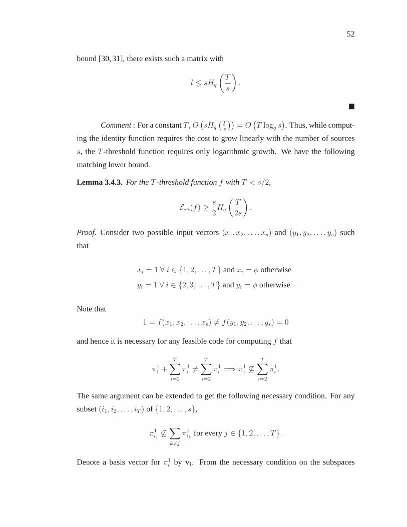
52

bound [30,31], there exists such a matrix with

l ≤ sHq

(T

s

).

Comment: For a constantT ,O(sHq

(Ts

))= O

(T logq s

). Thus, while comput-

ing the identity function requires the cost to grow linearlywith the number of sources

s, theT -threshold function requires only logarithmic growth. We have the following

matching lower bound.

Lemma 3.4.3.For theT -threshold functionf with T < s/2,

Emin(f) ≥ s

2Hq

(T

2s

).

Proof. Consider two possible input vectors(x1, x2, . . . , xs) and (y1, y2, . . . , ys) such

that

xi = 1 ∀ i ∈ 1, 2, . . . , T andxi = φ otherwise

yi = 1 ∀ i ∈ 2, 3, . . . , T andyi = φ otherwise.

Note that

1 = f(x1, x2, . . . , xs) 6= f(y1, y2, . . . , ys) = 0

and hence it is necessary for any feasible code for computingf that

π11 +

T∑

i=2

π1i 6=

T∑

i=2

π1i =⇒ π1

1 6⊆T∑

i=2

π1i .

The same argument can be extended to get the following necessary condition. For any

subset(i1, i2, . . . , iT ) of 1, 2, . . . , s,

π1ij6⊆∑

k 6=j

π1ik

for everyj ∈ 1, 2, . . . , T.

Denote a basis vector forπ1i by vi. From the necessary condition on the subspaces

53

π11, π

12, . . . , π

1s , any collection ofT vectors fromv1,v2, . . . ,vs are linearly independent.

The l × s matrix with the vectorsv1,v2, . . . ,vs as columns corresponds to the parity

check matrix of aq-ary linear code of lengths and minimum distance at leastT + 1.

Using the bounds in [30,31], forT < s/2 we have

l ≥ sHq

(T

2s

)− 1

2logq

(4T

(1− T

2s

)).

The result then follows since

1

2logq

(4T

(1− T

2s

))≤ s

2Hq

(T

2s

). (3.8)

For s ≤ 11, (3.8) can be verified numerically. Lets ≥ 12. Then (3.8) holds if we show

that for every1 ≤ T < s/2,

s · T2s

ln

(2s

T

)≥ ln(4T ) or equivalently,

T ln

(2s

T

)− 2 ln(4T ) ≥ 0. (3.9)

For T = 1, (3.9) holds sinces ≥ 8. Differentiating the left-hand side of (3.9) with

respect toT , we get

ln(2s)− ln(T )− 1− 2

T

which is greater than zero sinces ≥ 12 andT ≤ s/2. Thus, (3.9) is true for every

1 ≤ T < s/2 and thus (3.8) holds.

3.4.2 Maximum Function

Lemma 3.4.4.There exists a(1, l) feasible code for computing the maximum function

such that

l ≤ min|A| , s+ ⌈logq |A|⌉)

.

Proof. Consider the following two schemes for computing the maximumfunction.

• A (1, |A|) scheme: Let v1,v2, . . . ,v|A| be linearly independent vectors of length|A|each. For every sourceσi, let Ci =

(v1,v2, . . . ,v|A|

). This scheme hasl = |A|.

54

• A (1, s + ⌈logq |A|⌉) scheme: We can compute the identity function withl = s +

⌈logq |A|⌉ and hence can compute the maximum function also. This schemeis useful if

A ≥ s.

Comment: Thus when|A| ≪ s, the first scheme is much more efficient than

reconstructing all the source messages.

Lemma 3.4.5.For the maximum target functionf ,

Emin(f) ≥ min|A| , s.

Proof. LetA =(a1, a2, . . . , a|A|

)be an ordered set (in decreasing order) and letM =

min|A| , s. Consider an input vectorx such that

(x)i = ai ∀ i ∈ 1, . . . ,M and(x)i = φ otherwise

and a collection ofM indicesi1, i2, . . . , iM such that eachij = j. Then from (3.5), it

can be easily verified that the maximum target functionf satisfies propertyQ(M). The

result then follows from Lemma 3.3.4.

3.4.3 K-largest Values Function

LetA = (a1, a2, . . . , a|A|) be an ordered set (in increasing order). For any given

input vector(x1, x2, . . . , xs), let (x1, x2, . . . , xs) denote the vector which is a permuta-

tion of the input vector and satisfiesxi ≥ xi+1 for eachi. Then theK-largest values

function is given by

f (x1, x2, . . . , xs) = (x1, x2, . . . , xK) .

Lemma 3.4.6. There exists a(1, l) feasible code for computing theK-largest values

function withK < N/2, such that

l ≤ |A| · sHq

(K

2s

).

55

• Let H be the(l/ |A|)× s parity check matrix of a

binary code with minimum distanceK + 1.

• If sourceσi takes valueaj from the alphabetA, then it

transmits a vector which is all zero except the

(j − 1)× (l/ |A|) + 1 to j × (l/ |A|) elements,

which take values from thei-th column ofH.

• Each vector in the union subspaceΠ that the sink

receives is parsed into|A| sub-vectors of lengthl/ |A|.• Let Πj ⊆ F

l/|A|q denote the subspace spanned by

collecting thej-th sub-vector of each vector inΠ.

• Thus by calculatingdim(Π|A|), dim(Π|A|−1) . . . ,

the sink can compute theK largest values.

Figure 3.3: A (1, l) code forK-largest values function

Proof. Consider the scheme in Figure 3.3.

Again from [30,31], there exists a parity check matrix such that

l

|A| ≤ sHq

(K

2s

).

Comment: Again, for constant|A| andK, the cost only grows logarithmically

with the number of sourcess.

Lemma 3.4.7.For theK-largest values target functionf withK < s/2,

Emin(f) ≥ s

2Hq

(K

2s

).

Proof. If the receiver can correctly compute theK-largest values, then it can also deduce

if the number of active sources is greater thanK or not. Thus, it can also compute

the T -threshold function with the thresholdT = K. The result then follows from

Lemma 3.4.3.

56

3.5 A general scheme for computation

We now present a general method to compute functions under our network

model. We will illustrate the method for boolean functions of the form f : As →0, 1. For a general function, the output can be considered as a string of bits and the

above scheme can be used separately to compute each bit of theoutput.

Sincef has boolean output, it can be written as

f (x1, x2, . . . , xs) =s∑

i=1

s∏

j=1

Bij

wheres is some integer such that1 ≤ s ≤ |A|s; Bij are boolean variables such that

the value ofBij depends only onxj; and the sum and product represent boolean OR and

AND. By taking the complement, we have

f (x1, x2, . . . , xs) =s∏

i=1

s∑

j=1

Bij.

Given any inputxj, sourcej creates a vectorvj of lengths such thati-th component is

Bij. Each sourcej then sends the corresponding vectorvj into the network and the sink

collects linear combinations of these vectors. If thei-th component of any of the vectors

in the union subspace at the sink is1, then a boolean variableAi is assigned the value1.

This implies that

Ai =s∑

j=1

Bij

and hence,

f (x1, x2, . . . , xs) =s∏

i=1

Ai.

Thus, we have a(1, s) scheme to compute any functionf with binary output.

Comment: Since the cost associated with the above code iss, the above scheme

is efficient when the number of input vectors for which the function value is1 (or 0) is

much smaller than the total number of possible input vectors.

We now present an example to illustrate the above method.

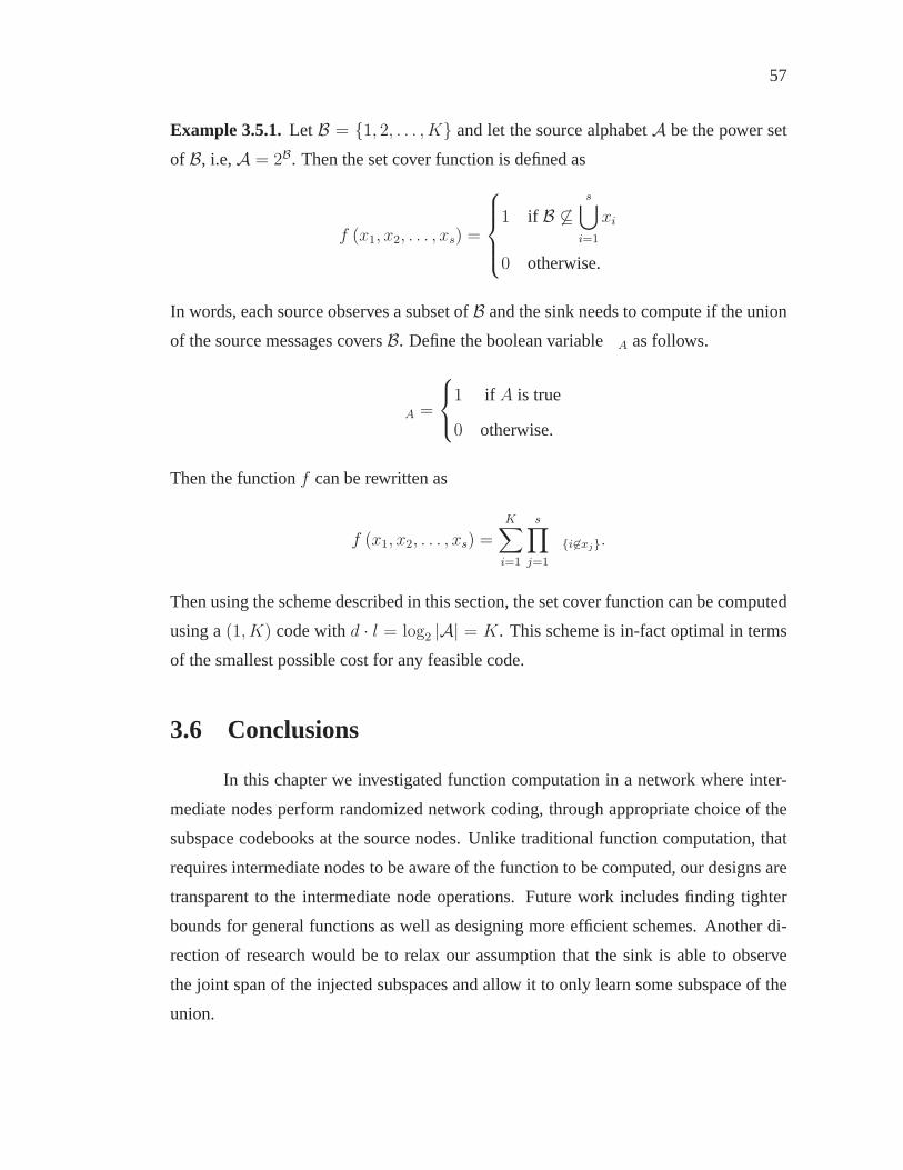
57

Example 3.5.1.Let B = 1, 2, . . . , K and let the source alphabetA be the power set

of B, i.e,A = 2B. Then the set cover function is defined as

f (x1, x2, . . . , xs) =

1 if B 6⊆s⋃

i=1

xi

0 otherwise.

In words, each source observes a subset ofB and the sink needs to compute if the union

of the source messages coversB. Define the boolean variable1A as follows.

1A =

1 if A is true

0 otherwise.

Then the functionf can be rewritten as

f (x1, x2, . . . , xs) =K∑

i=1

s∏

j=1

1i6∈xj.

Then using the scheme described in this section, the set cover function can be computed

using a(1, K) code withd · l = log2 |A| = K. This scheme is in-fact optimal in terms

of the smallest possible cost for any feasible code.

3.6 Conclusions

In this chapter we investigated function computation in a network where inter-

mediate nodes perform randomized network coding, through appropriate choice of the

subspace codebooks at the source nodes. Unlike traditionalfunction computation, that

requires intermediate nodes to be aware of the function to becomputed, our designs are

transparent to the intermediate node operations. Future work includes finding tighter

bounds for general functions as well as designing more efficient schemes. Another di-

rection of research would be to relax our assumption that thesink is able to observe

the joint span of the injected subspaces and allow it to only learn some subspace of the

union.

58

Chapter 3, in part, has been submitted for publication of the material. The dis-

sertation author was a primary investigator and author of this paper.

Chapter 4

Repeated Computation: Network

Coding for Computing

The followingnetwork computingproblem is considered. Source nodes in a di-

rected acyclic network generate independent messages and asingle receiver node com-

putes a target functionf of the messages. The objective is to maximize the average

number of timesf can be computed per network usage, i.e., the “computing capacity”.

Thenetwork codingproblem for a single-receiver network is a special case of the net-

work computing problem in which all of the source messages must be reproduced at

the receiver. For network coding with a single receiver, routing is known to achieve

the capacity by achieving the networkmin-cutupper bound. We extend the definition

of min-cut to the network computing problem and show that themin-cut is still an up-

per bound on the maximum achievable rate and is tight for computing (using coding)

any target function in multi-edge tree networks and for computing linear target func-

tions in any network. We also study the bound’s tightness fordifferent classes of target

functions.

59

60

4.1 Introduction

We consider networks where source nodes generate independent messages and

a single receiver node computes a target functionf of these messages. The objective is

to characterize the maximum rate of computation, that is themaximum number of times

f can be computed per network usage.

Giridhar and Kumar [3] have recently stated:

“In its most general form, computing a function in a network involves com-municating possibly correlated messages, to a specific destination, at a de-sired fidelity with respect to a joint distortion criterion dependent on thegiven function of interest. This combines the complexity ofsource codingof correlated sources, with rate distortion, different possible network collab-orative strategies for computing and communication, and the inapplicabilityof the separation theorem demarcating source and channel coding.”

The overwhelming complexity of network computing suggeststhat simplifications be

examined in order to obtain some understanding of the field.

We present a natural model of network computing that is closely related to the

network coding model of Ahlswede, Cai, Li, and Yeung [32, 33].Network coding is a

widely studied communication mechanism in the context of network information the-

ory. In network coding, some nodes in the network are labeledas sources and some as

receivers. Each receiver needs to reproduce a subset of the messages generated by the

source nodes, and all nodes can act as relays and encode the information they receive on

in-edges, together with the information they generate if they are sources, into codewords

which are sent on their out-edges. In existing computer networks, the encoding opera-

tions are purely routing: at each node, the codeword sent over an out-edge consists of a

symbol either received by the node, or generated by it if it isa source. It is known that

allowing more complex encoding than routing can in general be advantageous in terms

of communication rate [32, 34, 35]. Network coding with a single receiver is equiva-

lent to a special case of our function computing problem, namely when the function to

be computed is the identity, that is when the receiver wants to reproduce all the mes-

sages generated by the sources. In this chapter, we study network computation for target

functions different than the identity.

61

Some other approaches to network computation have also appeared in the litera-

ture. In [28,29,36–39] network computing was considered asan extension of distributed

source coding, allowing the sources to have a joint distribution and requiring that a func-

tion be computed with small error probability. For example,[36] considered a network

where two correlated uniform binary sources are both connected to the receiver and de-

termine the maximum rate of computing the parity of the messages generated by the

two sources. A rate-distortion approach to the problem has been studied in [40–42].

However, the complexity of network computing has restricted prior work to the analysis

of elementary networks. Networks with noisy links were studied in [6–8,10,12,43–46].

For example, [6] considered broadcast networks where any transmission by a node is re-

ceived by each of its neighbors via an independent binary symmetric channel. Random-

ized gossip algorithms [47] have been proposed as practicalschemes for information

dissemination in large unreliable networks and were studied in the context of distributed

computation in [47–52].

In the present chapter, our approach is somewhat (tangentially) related to the

field of communication complexity [1, 53] which studies the minimum number of mes-

sages that two nodes need to exchange in order to compute a function of their inputs

with zero error. Other studies of computing in networks havebeen considered in [3, 4],

but these were restricted to the wireless communication protocol model of Gupta and

Kumar [2].

In contrast, our approach is more closely associated with wired networks with

independent noiseless links. Our work is closest in spirit to the recent work of [54–57]

on computing the sum (over a finite field) of source messages innetworks. We note that

in independent work, Kowshik and Kumar [58] obtain the asymptotic maximum rate of

computation in tree networks and present bounds for computation in networks where all

nodes are sources.

Our main contributions are summarized in Section 4.1.3, after formally intro-

ducing the network model.

62

4.1.1 Network model and definitions

In this chapter, anetworkN consists of a finite, directed acyclic multigraph

G = (V , E), a set ofsource nodesS = σ1, . . . , σs ⊆ V, and areceiverρ ∈ V. Such

a network is denoted byN = (G,S, ρ). We will assume thatρ 6∈ S and that the graph1

G contains a directed path from every node inV to the receiverρ. For each nodeu ∈ V,

let Ei(u) andEo(u) denote the set of in-edges and out-edges ofu respectively. We will

also assume (without loss of generality) that if a network node has no in-edges, then it

is a source node.

An alphabetA is a finite set of size at least two. For any positive integerm, any

vectorx ∈ Am, and anyi ∈ 1, 2, . . . ,m, let xi denote thei-th component ofx. For

any index setI = i1, i2, . . . , iq ⊆ 1, 2, . . . ,m with i1 < i2 < . . . < iq, letxI denote

the vector(xi1 , xi2 , . . . , xiq) ∈ A|I|.

Thenetwork computingproblem consists of a networkN and atarget function

f of the form

f : As −→ B

(see Table 4.1 for some examples). We will also assume that any target function de-

pends on all network sources (i.e. they cannot be constant functions of any one of their

arguments). Letk andn be positive integers. Given a networkN with source setS and

alphabetA, amessage generatoris any mapping

α : S −→ Ak.

For eachi, α(σi) is called amessage vectorand its componentsα(σi)1 , . . . , α(σi)k are

calledmessages.2

Definition 4.1.1. A (k, n) network codefor computing a target functionf in a network

N consists of the following:

1Throughout the chapter, we will use “graph” to mean a directed acyclic multigraph, and “network”to mean a single-receiver network. We may sometimes writeE(G) to denote the edges of graphG.

2For simplicity, we assume that each source has exactly one message vector associated with it, but allof the results in this chapter can readily be extended to the more general case.

63

(i) For any nodev ∈ V − ρ and any out-edgee ∈ Eo(v), anencoding function:

h(e) :

∏

e∈Ei(v)

An

×Ak −→ An if v is a source node

∏

e∈Ei(v)

An −→ An otherwise.

(ii) A decoding function:

ψ :

|Ei(ρ)|∏

j=1

An −→ Bk.

Given a(k, n) network code, every edgee ∈ E carries a vectorze of at most

n alphabet symbols3, which is obtained by evaluating the encoding functionh(e) on the

set of vectors carried by the in-edges to the node and the node’s message vector if it

is a source. The objective of the receiver is to compute the target functionf of the

source messages, for any arbitrary message generatorα. More precisely, the receiver

constructs a vector ofk alphabet symbols such that for eachi ∈ 1, 2, . . . , k, the i-

th component of the receiver’s computed vector equals the value of the desired target

functionf applied to thei-th components of the source message vectors, for any choice

of message generatorα. Let e1, e2, . . . , e|Ei(ρ)| denote the in-edges of the receiver.

Definition 4.1.2. A (k, n) network code is calleda solution for computingf in N(or simply a (k, n) solution) if the decoding functionψ is such that for eachj ∈1, 2, . . . , k and for every message generatorα, we have

ψ(ze1 , · · · , ze|Ei(ρ)|

)

j= f

(α(σ1)j , · · · , α(σs)j

). (4.1)

If there exists a(k, n) solution, we say the rational numberk/n is anachievable com-

puting rate.

In the network coding literature, one definition of thecoding capacityof a net-

work is the supremum of all achievable coding rates [59, 60].We adopt an analogous

definition for computing capacity.

3By default, we will assume that edges carry exactlyn symbols.

64

Table 4.1: Examples of target functions.

Target functionf AlphabetA f (x1, . . . , xs) Comments

identity arbitrary (x1, . . . , xs)

arithmetic sum 0, . . . , q − 1 x1 + · · ·+ xs ‘+’ is ordinary integer addition

modr sum 0, . . . , q − 1 x1 ⊕ . . .⊕ xs ⊕ is mod r addition

histogram 0, . . . , q − 1 (c0, . . . , cq−1) ci = |j : xj = i| ∀ i ∈ Alinear finite field a1x1 + . . . + asxs arithmetic performed in the field

maximum ordered set max x1, . . . , xs

Definition 4.1.3. Thecomputing capacityof a networkN with respect to target function

f is

Ccod(N , f) = sup

k

n: ∃ (k, n) network code for computingf in N

.

Thus, the computing capacity is the supremum of all achievable computing rates

for a given networkN and a target functionf . Some example target functions are

defined in Table 4.1.

Definition 4.1.4. For any target functionf : As −→ B, any index setI ⊆ 1, 2, . . . , s,and anya, b ∈ A|I|, we write a ≡ b if for every x, y ∈ As, we havef(x) = f(y)

wheneverxI = a, yI = b, andxj = yj for all j 6∈ I.

It can be verified that≡ is an equivalence relation4 for everyf andI.

Definition 4.1.5. For everyf andI, let RI,f denote the total number of equivalence

classes induced by≡ and let

ΦI,f : A|I| −→ 1, 2, . . . , RI,f4Witsenhausen [27] represented this equivalence relation in terms of the independent sets of a char-

acteristic graph and his representation has been used in various problems related to function computa-tion [28, 29, 37]. Although≡ is defined with respect to a particular index setI and a functionf , we donot make this dependence explicit – the values ofI andf will be clear from the context.

65

be any function such thatΦI,f (a) = ΦI,f (b) iff a ≡ b.

That is,ΦI,f assigns a unique index to each equivalence class, and

RI,f =∣∣ΦI,f (a) : a ∈ A|I|∣∣ .

The value ofRI,f is independent of the choice ofΦI,f . We callRI,f the footprint size

of f with respect toI.

Remark 4.1.6. Let Ic = 1, 2, . . . , s − I. The footprint sizeRI,f has the following

interpretation. Suppose a network has two nodes,X andY , and both are sources. A

single directed edge connectsX to Y . Let X generatex ∈ A|I| andY generatey ∈A|Ic|. X communicates a functiong(x) of its input, toY so thatY can computef(a)

wherea ∈ As, aI = x, andaIc = y. Then for anyx, x ∈ A|I| such thatx 6≡ x, we

needg(x) 6= g(x). Thus∣∣g(A|I|)∣∣ ≥ RI,f , which implies a lower bound on a certain

amount of “information” thatX needs to send toY to ensure that it can compute the

functionf . Note thatg = ΦI,f achieves the lower bound. We will use this intuition to

establish a cut-based upper bound on the computing capacityCcod(N , f) of any network

N with respect to any target functionf , and to devise a capacity-achieving scheme for

computing any target function in multi-edge tree networks.

Definition 4.1.7. A set of edgesC ⊆ E in networkN is said toseparatesources

σm1 , . . . , σmdfrom the receiverρ, if for each i ∈ 1, 2, . . . , d, every directed path

from σmito ρ contains at least one edge inC. The setC is said to be acut in N if it

separates at least one source from the receiver. For any networkN , defineΛ(N ) to be

the collection of all cuts inN . For any cutC ∈ Λ(N ) and any target functionf , define

IC = i : C separatesσi from the receiverRC,f = RIC ,f . (4.2)

Since target functions depend on all sources, we haveRC,f ≥ 2 for any cutC

and any target functionf . The footprint sizesRC,f for some example target functions

are computed below.

66

A multi-edge treeis a graph such that for every nodev ∈ V, there exists a nodeu

such that all the out-edges ofv are in-edges tou, i.e.,Eo(v) ⊆ Ei(u) (e.g. see Figure 4.1).

Figure 4.1: An example of a multi-edge tree.

4.1.2 Classes of target functions

We study the following four classes of target functions: (1)divisible, (2) sym-

metric, (3)λ-exponential, (4)λ-bounded.

Definition 4.1.8. A target functionf : As −→ B is divisible if for every index set

I ⊆ 1, . . . , s, there exists a finite setBI and a functionf I : A|I| −→ BI such that the

following hold:

(1) f 1,...,s = f

(2)∣∣f I(A|I|)∣∣ ≤ |f (As)|

(3) For every partitionI1, . . . , Iγ of I, there exists a function

g : BI1 × · · · × BIγ −→ BI such that for everyx ∈ A|I|, we have

f I(x) = g(f I1(xI1) , . . . , f

Iγ(xIγ

)).

Examples of divisible target functions include the identity, maximum,mod r

sum, and arithmetic sum.

Divisible functions have been studied previously5 by Giridhar and Kumar [3]

and Subramanian, Gupta, and Shakkottai [4]. Divisible target functions can be com-

puted in networks in a divide-and-conquer fashion as follows. For any arbitrary partition

5The definitions in [3,4] are similar to ours but slightly morerestrictive.

67

I1, . . . , Iγ of the source indices1, . . . , s, the receiverρ can evaluate the target func-

tion f by combining evaluations off I1 , . . . , f Iγ . Furthermore, for everyi = 1, . . . , γ,

the target functionf Ii can be evaluated similarly by partitioningIi and this process can

be repeated until the function value is obtained.

Definition 4.1.9. A target functionf : As −→ B is symmetricif for any permutationπ

of 1, 2, . . . , s and any vectorx ∈ As,

f(x1, x2, . . . , xs) = f(xπ(1), xπ(2), . . . , xπ(s)).

That is, the value of a symmetric target function is invariant with respect to the

order of its arguments and hence, it suffices to evaluate the histogram target function for

computing any symmetric target function. Examples of symmetric functions include the

arithmetic sum, maximum, andmod r sum. Symmetric functions have been studied in

the context of computing in networks by Giridhar and Kumar [3], Subramanian, Gupta,

and Shakkottai [4], Ying, Srikant, and Dullerud [10], and [43].

Definition 4.1.10. Let λ ∈ (0, 1]. A target functionf : As −→ B is said to beλ-

exponentialif its footprint size satisfies

RI,f ≥ |A|λ|I| for everyI ⊆ 1, 2, . . . , s.

Let λ ∈ (0,∞). A target functionf : As −→ B is said to beλ-boundedif its footprint

size satisfies

RI,f ≤ |A|λ for everyI ⊆ 1, 2, . . . , s.

Example 4.1.11.The following facts are easy to verify:

• The identity function is1-exponential.

• LetA be an ordered set. The maximum (or minimum) function is1-bounded.

• Let A = 0, 1, . . . , q − 1 whereq ≥ 2. Themod r sum target function with

q ≥ r ≥ 2 is logq r-bounded.

68

Remark 4.1.12.Giridhar and Kumar [3] defined two classes of functions:type-threshold

andtype-sensitivefunctions. Both are sub-classes of symmetric functions. In addition,

type-threshold functions are also divisible andc-bounded, for some constantc that is

independent of the network size. However, [3] uses a model ofinterference for simulta-

neous transmissions and their results do not directly compare with ours.

Following the notation in Leighton and Rao [61], themin-cutof any networkNwith unit-capacity edges is

min-cut(N ) = minC∈Λ(N )

|C||IC |

. (4.3)

A more general version of the network min-cut plays a fundamental role in the field of

multi-commodity flow [61,62]. The min-cut provides an upperbound on the maximum

flow for any multi-commodity flow problem. The min-cut is alsoreferred to as “spar-

sity” by some authors, such as Harvey, Kleinberg, and Lehman[34] and Vazirani [62].

We next generalize the definition in (4.3) to the network computing problem.

Definition 4.1.13. If N is a network andf is a target function, then define

min-cut(N , f) = minC∈Λ(N )

|C|log|A|RC,f

. (4.4)

Example 4.1.14.

• If f is the identity target function, then

min-cut(N , f) = minC∈Λ(N )

|C||IC |

.

Thus for the identity function, the definition of min-cut in (4.3) and (4.4) coincide.

• LetA = 0, 1, . . . , q − 1. If f is the arithmetic sum target function, then

min-cut(N , f) = minC∈Λ(N )

|C|logq ((q − 1) |IC |+ 1)

. (4.5)

69

• LetA be an ordered set. Iff is the maximum target function, then

min-cut(N , f) = minC∈Λ(N )

|C| .

4.1.3 Contributions

The main results of this chapter are as follows. In Section 4.2, we show (Theo-

rem 4.2.1) that for any networkN and any target functionf , the quantity min-cut(N , f)

is an upper bound on the computing capacityCcod(N , f). In Section 4.3, we note that

the computing capacity for any network with respect to the identity target function is

equal to the min-cut upper bound (Theorem 4.3.1). We show that the min-cut bound on

computing capacity can also be achieved for all networks with linear target functions

over finite fields (Theorem 5.5.6) and for all multi-edge treenetworks with any target

function (Theorem 4.3.3). For any network and any target function, a lower bound on

the computing capacity is given in terms of the Steiner tree packing number (Theo-

rem 4.3.5). Another lower bound is given for networks with symmetric target functions

(Theorem 4.3.7). In Section 4.4, the tightness of the above-mentioned bounds is ana-

lyzed for divisible (Theorem 4.4.2), symmetric (Theorem 4.4.3),λ-exponential (Theo-

rem 4.4.4), andλ-bounded (Theorem 4.4.5) target functions. Forλ-exponential target

functions, the computing capacity is at leastλ times the min-cut. If every non-receiver

node in a network is a source, then forλ-bounded target functions the computing capac-

ity is at least a constant times the min-cut divided byλ. It is also shown, with an example

target function, that there are networks for which the computing capacity is less than an

arbitrarily small fraction of the min-cut bound (Theorem 4.4.7). In Section 4.5, we dis-

cuss an example network and target function in detail to illustrate the above bounds. In

Section 4.6, conclusions are given and various lemmas are proven in the Appendix.

4.2 Min-cut upper bound on computing capacity

The following shows that the maximum rate of computing a target functionf in

a networkN is at most min-cut(N , f).

70

Theorem 4.2.1.If N is a network with target functionf , then

Ccod(N , f) ≤ min-cut(N , f).

Proof. Let the network alphabet beA and consider any(k, n) solution for computing

f in N . Let C be a cut and for eachi ∈ 1, 2, . . . , k, let a(i), b(i) ∈ A|IC |. Suppose

j ∈ 1, 2, . . . , k is such thata(j) 6≡ b(j), where≡ is the equivalence relation from

Definition 4.1.4. Then there existx, y ∈ As satsifying: f(x) 6= f(y), xIC= a(j),

yIC= b(j), andxi = yi for everyi 6∈ IC .

The receiverρ can compute the target functionf only if, for every such paira(1), . . . , a(k)

and

b(1), . . . , b(k)

corresponding to the message vectors generated by

the sources inIC , the edges in cutC carry distinct vectors. Since the total number of

equivalence classes for the relation≡ equals the footprint sizeRC,f , the edges in cutC

should carry at least(RC,f )k distinct vectors. Thus, we have

An|C| ≥ (RC,f )k

and hence for any cutC,k

n≤ |C|

log|A|RC,f

.

Since the cutC is arbitrary, the result follows from Definition 5.2.6 and (4.4).

The min-cut upper bound has the following intuition. Given any cutC ∈ Λ(N ),

at leastlog|A|RC,f units of information need to be sent across the cut to successfully

compute a target functionf . In subsequent sections, we study the tightness of this

bound for different classes of functions and networks.

4.3 Lower bounds on the computing capacity

The following result shows that the computing capacity of any networkN with

respect to the identity target function equals the coding capacity for ordinary network

coding.

71

Theorem 4.3.1.If N is a network with the identity target functionf , then

Ccod(N , f) = min-cut(N , f) = min-cut(N ).

Proof. Rasala Lehman and Lehman [63, p.6, Theorem 4.2] showed that for any single-

receiver network, the conventional coding capacity (when the receiver demands the mes-

sages generated by all the sources) always equals the min-cut(N ). Since the target func-

tion f is the identity, the computing capacity is the coding capacity and min-cut(N , f)

= min-cut(N ), so the result follows.

Theorem 4.3.2.If N is a network with a finite field alphabet and with a linear target

functionf , then

Ccod(N , f) = min-cut(N , f).

Proof. The proof of this result is relegated to Section 5.5. It also follows from [56,

Theorem 2].

Theorems 4.3.1 and 5.5.6 demonstrate the achievability of the min-cut bound

for arbitrary networks with particular target functions. In contrast, the following result

demonstrates the achievability of the min-cut bound for arbitrary target functions and a

particular class of networks. The following theorem concerns multi-edge tree networks,

which were defined in Section 4.1.1.

Theorem 4.3.3.If N is a multi-edge tree network with target functionf , then

Ccod(N , f) = min-cut(N , f).

Proof. Let A be the network alphabet. From Theorem 4.2.1, it suffices to show that

Ccod(N , f) ≥ min-cut(N , f). SinceEo(v) is a cut for nodev ∈ V − ρ, and using (4.2),

we have

min-cut(N , f) ≤ minv ∈ V−ρ

|Eo(v)|log|A|REo(v),f

. (4.6)

72

Consider any positive integersk, n such that

k

n≤ min

v ∈ V−ρ

|Eo(v)|log|A|RIEo(v),f

. (4.7)

Then we have

|A||Eo(v)|n ≥ RkIEo(v),f

for every nodev ∈ V − ρ. (4.8)

We outline a(k, n) solution for computingf in the multi-edge tree networkN . Each

sourceσi ∈ S generates a message vectorα(σi) ∈ Ak. Denote the vector ofi-th

components of the source messages by

x(i) = (α(σ1)i , · · · , α(σs)i) .

Every nodev ∈ V −ρ sends out a unique index (as guaranteed by (4.8)) overA|Eo(v)|n

corresponding to the set of equivalence classes

ΦIEo(v),f (x(l)IEo(v)

) for l ∈ 1, · · · , k. (4.9)

If v has no in-edges, then by assumption, it is a source node, sayσj. The set of

equivalence classes in (4.9) is a function of its own messagesα(σj)l for l ∈ 1, . . . , k.On the other hand ifv has in-edges, then letu1, u2, · · · , uj be the nodes with out-edges

to v. For eachi ∈ 1, 2, · · · , j, using the uniqueness of the index received fromui,

nodev recovers the equivalence classes

ΦIEo(ui),f (x

(l)IEo(ui)

) for l ∈ 1, · · · , k. (4.10)

Furthermore, the equivalence classes in (4.9) can be identified byv from the equivalance

classes in (4.10) (andα(v) if v is a source node) using the fact that for a multi-edge tree

networkN , we have a disjoint union

IEo(v) =

j⋃

i=1

IEo(ui).

If each nodev follows the above steps, then the receiverρ can identify the equiv-

73

alence classesΦIEi(ρ),f

(x(i))

for i ∈ 1, . . . , k. The receiver can evaluatef(x(l)) for

eachl from these equivalence classes. The above solution achieves a computing rate of

k/n. From (4.7), it follows that

Ccod(N , f) ≥ minv ∈ V−ρ

|Eo(v)|log|A|RIEo(v),f

. (4.11)

We next establish a general lower bound on the computing capacity for arbitrary

target functions (Theorem 4.3.5) and then another lower bound specifically for symmet-

ric target functions (Theorem 4.3.7).

For any networkN = (G,S, ρ) with G = (V , E), define aSteiner tree6 of N to

be a minimal (with respect to nodes and edges) subgraph ofG containingS andρ such

that every source inS has a directed path to the receiverρ. Note that every non-receiver

node in a Steiner tree has exactly one out-edge. LetT (N ) denote the collection of all

Steiner trees inN . For each edgee ∈ E(G), let Je = i : ti ∈ T (N ) ande ∈ E(ti).Thefractional Steiner tree packing numberΠ(N ) is defined as the linear program

Π(N ) = max∑

ti∈T (N )

ui subject to

ui ≥ 0 ∀ ti ∈ T (N ),∑

i∈Je

ui ≤ 1 ∀ e ∈ E(G).(4.12)

Note thatΠ(N ) ≥ 1 for any networkN , and the maximum value of the sum in (4.12)

is attained at one or more vertices of the closed polytope corresponding to the linear

constraints. Since all coefficients in the constraints are rational, the maximum value

in (4.12) can be attained with rationalui’s. The following theorem provides a lower

bound7 on the computing capacity for any networkN with respect to a target function

f and uses the quantityΠ(N ). In the context of computing functions,ui in the above

6Steiner trees are well known in the literature for undirected graphs. For directed graphs a “Steinertree problem” has been studied and our definition is consistent with such work (e.g., see [64]).

7In order to compute the lower bound, the fractional Steiner tree packing numberΠ(N ) can be eval-uated using linear programming. Also note that if we construct thereverse multicast networkby lettingeach source in the original networkN become a receiver, letting the receiver in theN become the onlysource, and reversing the direction of each edge, then it canbe verified that the routing capacity for thereverse multicast network is equal toΠ(N ).

74

linear program indicates the fraction of the time the edges in treeti are used to compute

the desired function. The fact that every edge in the networkhas unit capacity implies∑

i∈Jeui ≤ 1.

Lemma 4.3.4.For any Steiner treeG′ of a networkN , letN ′ = (G′, S, ρ). LetC ′ be a

cut inN ′. Then there exists a cutC in N such thatIC = IC′.

(Note thatIC′ is the set indices of sources separated inN ′ by C ′. The setIC′

may differ from the indices of sources separated inN byC ′.)

Proof. Define the cut

C =⋃

i′∈IC′

Eo(σi′). (4.13)

C is the collection of out-edges inN of a set of sources disconnected by the cutC ′ in

N ′. If i ∈ IC′, then, by (4.13),C disconnectsσi from ρ in N , and thusIC′ ⊆ IC .

Let σi be a source. such thati ∈ IC and LetP be a path fromσi to ρ in N .

From (4.13), it follows that there existsi′ ∈ IC′ such thatP contains at least one edge in

Eo(σi′). If P also lies inN ′ and does not contain any edge inC ′, thenσi′ has a path to

ρ in N ′ that does not contain any edge inC ′, thus contradicting the fact thatσi′ ∈ IC′.

Therefore, eitherP does not lie inN ′ or P contains an edge inC ′. Thusσi ∈ IC′, i.e.,

IC ⊆ IC′.

Theorem 4.3.5.If N is a network with alphabetA and target functionf , then

Ccod(N , f) ≥ Π(N ) · minC∈Λ(N )

1

log|A|RC,f

.

Proof. SupposeN = (G,S, ρ). Consider a Steiner treeG′ = (V ′, E ′) of N , and let

N ′ = (G′, S, ρ). From Lemma 4.3.4 (takingC ′ to beEo(v) in N ′), we have

∀ v ∈ V ′ − ρ, ∃ C ∈ Λ(N ) such thatI ′Eo(v) = IC . (4.14)

Now we lower bound the computing capacity for the networkN ′ with respect to target

75

functionf .

Ccod(N ′, f)

= min-cut(N ′, f) [from Theorem 4.3.3] (4.15)

= minv ∈ V ′−ρ

1

log|A|RI′Eo(v)

,f

[from Theorem 4.2.1, (4.6), (4.11)]

≥ minC∈Λ(N )

1

log|A|RIC ,f

[from (4.14)]. (4.16)

The lower bound in (4.16) is the same for every Steiner tree ofN . We will use this

uniform bound to lower bound the computing capacity forN with respect tof . Denote

the Steiner trees ofN by t1, . . . , tT . Let ǫ > 0 and letr denote the quantity on the

right hand side of (4.16). On every Steiner treeti, a computing rate of at leastr − ǫ is

achievable by (4.16). Using standard arguments for time-sharing between the different

Steiner trees of the networkN , it follows that a computing rate of at least(r− ǫ) ·Π(N )

is achievable inN , and by lettingǫ→ 0, the result follows.

The lower bound in Theorem 4.3.5 can be readily computed and is sometimes

tight. The procedure used in the proof of Theorem 4.3.5 may potentially be improved

by maximizing the sum

∑

ti∈T (N )

ui ri subject to

ui ≥ 0 ∀ ti ∈ T (N ) ,∑

i∈Je

ui ≤ 1 ∀ e ∈ E(G)(4.17)

whereri is any achievable rate8 for computingf in the Steiner tree networkNi =

(ti, S, ρ).

We now obtain a different lower bound on the computing capacity in the special

case when the target function is the arithmetic sum. This lower bound is then used to give

an alternative lower bound (in Theorem 4.3.7) on the computing capacity for the class of

symmetric target functions. The bound obtained in Theorem 4.3.7 is sometimes better

than that of Theorem 4.3.5, and sometimes worse (Example 4.3.8 illustrates instances

8From Theorem 4.3.3,ri can be arbitrarily close to min-cut(ti, f).

76

of both cases).

Theorem 4.3.6.If N is a network with alphabetA = 0, 1, . . . , q − 1 and the arith-

metic sum target functionf , then

Ccod(N , f) ≥ minC∈Λ(N )

|C|logq Pq,s

wherePq,s denotes the smallest prime number greater thans(q − 1).

Proof. Let p = Pq,s and letN ′ denote the same network asN but whose alphabet isFp,

the finite field of orderp.

Let ǫ > 0. From Theorem 5.5.6, there exists a(k, n) solution for computing the

Fp-sum of the source messages inN ′ with an achievable computing rate satisfying

k

n≥ min

C∈Λ(N )|C| − ǫ.

This (k, n) solution can be repeated to derive a(ck, cn) solution for any integerc ≥ 1

(note that edges in the networkN carry symbols from the alphabetA = 0, 1, . . . , q −1, while those in the networkN ′ carry symbols from a larger alphabetFp). Any

(ck, cn) solution for computing theFp-sum inN ′ can be ‘simulated’ in the network

N by a(ck, ⌈cn logq p⌉

)code (e.g. see [65]). Furthermore, sincep ≥ s(q − 1) + 1 and

the source alphabet is0, 1, . . . , q − 1, theFp-sum of the source messages in network

N is equal to their arithmetic sum. Thus, by choosingc large enough, the arithmetic

sum target function is computed inN with an achievable computing rate of at least

minC∈Λ(N )

|C|

logq p− 2ǫ.

Sinceǫ is arbitrary, the result follows.

Theorem 4.3.7.If N is a network with alphabetA = 0, 1, . . . , q−1 and a symmetric

target functionf , then

Ccod(N , f) ≥min

C∈Λ(N )|C|

(q − 1) · logq P (s)

77

whereP (s) is the smallest prime number9 greater thans.

Proof. From Definition 4.1.9, it suffices to evaluate the histogram target functionf for

computingf . For any set of source messages(x1, x2, . . . , xs) ∈ As, we have

f (x1, . . . , xs) = (c0, c1, . . . , cq−1)

whereci = |j : xj = i| for eachi ∈ A. Consider the networkN ′ = (G,S, ρ) with

alphabetA′ = 0, 1. Then for eachi ∈ A, ci can be evaluated by computing the

arithmetic sum target function inN ′ where every source nodeσj is assigned the message

1 if xj = i, and0 otherwise. Since we know that

q−1∑

i=0

ci = s

the histogram target functionf can be evaluated by computing the arithmetic sum target

functionq−1 times in the networkN ′ with alphabetA′ = 0, 1. Let ǫ > 0. From The-

orem 4.3.6 in the Appendix, there exists a(k, n) solution for computing the arithmetic

sum target function inN ′ with an achievable computing rate of at least

k

n≥

minC∈Λ(N )

|C|

log2 P (s)− ǫ.

The above(k, n) solution can be repeated to derive a(ck, cn) solution for any in-

teger c ≥ 1. Note that edges in the networkN carry symbols from the alphabet

A = 0, 1, . . . , q − 1, while those in the networkN ′ carry symbols fromA′ = 0, 1.Any (ck, cn) code for computing the arithmetic sum function inN ′ can be simulated

in the networkN by a (ck, ⌈cn logq 2⌉) code10. Thus by choosingc large enough, the

above-mentioned code can be simulated in the networkN to derive a solution for com-9From Bertrand’s Postulate [66, p.343], we haveP (s) ≤ 2s.

10To see details of such a simulation, we refer the interested reader to [65].

78

puting the histogram target functionf with an achievable computing rate11 of at least

1

(q − 1)· 1

logq 2·

minC∈Λ(N )

|C|

log2 P (s)− 2ǫ.

Sinceǫ is arbitrary, the result follows.

σ1

σ1

σ2

σ2

N1

σ3

ρ

ρ

N2

Figure 4.2: The Reverse Butterfly NetworkN1 has two binary sourcesσ1, σ2 andnetworkN2 has three binary sourcesσ1, σ2, σ3, each withA = 0, 1. Each network’sreceiverρ computes the arithmetic sum of the source messages.

Example 4.3.8.Consider networksN1 andN2 in Figure 4.2, each with alphabetA =

0, 1 and the (symmetric) arithmetic sum target functionf . Theorem 4.3.7 provides

a larger lower bound on the computing capacityCcod(N1, f) than Theorem 4.3.5, but a

smaller lower bound onCcod(N2, f).

• For networkN1 (in Figure 4.2), we havemaxC∈Λ(N1)

RC,f = 3 and minC∈Λ(N1)

|C| = 2,

both of which occur, for example, whenC consists of the two in-edges to the

receiverρ. Also, (q − 1) logq P (s, q) = log2 3 andΠ(N1) = 3/2, so

Ccod(N1, f) ≥ (3/2)/ log2 3 [from Theorem 4.3.5]

Ccod(N1, f) ≥ 2/ log2 3 [from Theorem 4.3.7]. (4.18)

11Theorem 4.3.7 provides a uniform lower bound on the achievable computing rate for any symmetricfunction. Better lower bounds can be found by considering specific functions; for example Theorem 4.3.6gives a better bound for the arithmetic sum target function.

79

In fact, we get the upper boundCcod(N1, f) ≤ 2/ log2 3 from Theorem 4.2.1, and

thus from (4.18),Ccod(N1, f) = 2/ log2 3.

• For networkN2, we have maxC∈Λ(N2)

RC,f = 4 and minC∈Λ(N2)

|C| = 1, both of which

occur whenC = (σ3, ρ). Also, (q − 1) logq P (s, q) = log2 5 andΠ(N2) = 1,

so

Ccod(N2, f) ≥ 1/ log2 4 [from Theorem 4.3.5]

Ccod(N2, f) ≥ 1/ log2 5 [from Theorem 4.3.7].

From Theorem 4.3.3, we haveCcod(N2, f) = 1/ log2 4.

Remark 4.3.9. An open question, pointed out in [59], is whether the coding capacity

of a network can be irrational. Like the coding capacity, thecomputing capacity is the

supremum of ratiosk/n for which a(k, n) solution exists. Example 4.3.8 demonstrates

that the computing capacity of a network (e.g.N1) with unit capacity links can be

irrational when the target function is the arithmetic sum function.

4.4 On the tightness of the min-cut upper bound

In the previous section, Theorems 4.3.1 - 4.3.3 demonstrated three special in-

stances for which the min-cut(N , f) upper bound is tight. In this section, we use The-

orem 4.3.5 and Theorem 4.3.7 to establish further results onthe tightness of the min-

cut(N , f) upper bound for different classes of target functions.

The following lemma provides a bound on the footprint sizeRI,f for any divisi-

ble target functionf .

Lemma 4.4.1. For any divisible target functionf : As −→ B and any index setI ⊆1, 2, . . . , s, the footprint size satisfies

RI,f ≤ |f (As)| .

Proof. From the definition of a divisible target function, for anyI ⊆ 1, 2, . . . , s, there

80

exist mapsf I , f Ic, andg such that

f(x) = g(f I(xI), f

Ic

(xIc))∀ x ∈ As

whereIc = 1, 2, . . . , s − I. From the definition of the equivalence relation≡ (see

Definition 4.1.4), it follows thata, b ∈ A|I| belong to the same equivalence class when-

everf I(a) = f I(b). This fact implies thatRI,f ≤∣∣f I(A|I|)∣∣. We need

∣∣f I(A|I|)∣∣ ≤

|f (As)| to complete the proof which follows from Definition 4.1.8(2).

Theorem 4.4.2.If N is a network with a divisible target functionf , then

Ccod(N , f) ≥ Π(N )

|Ei(ρ)|·min-cut(N , f)

whereEi(ρ) denotes the set of in-edges of the receiverρ.

Proof. LetA be the network alphabet. From Theorem 4.3.5,

Ccod(N , f) ≥ Π(N ) · minC∈Λ(N )

1

log|A|RC,f

≥ Π(N ) · 1

log|A| |f (As)| [from Lemma 4.4.1]. (4.19)

On the other hand, for any networkN , the set of edgesEi(ρ) is a cut that separates the

set of sourcesS from ρ. Thus,

min-cut(N , f)

≤ |Ei(ρ)|log|A|REi(ρ),f

[from (4.4)]

=|Ei(ρ)|

log|A| |f (As)| [from IEi(ρ) = S and Definition 4.1.5]. (4.20)

Combining (4.19) and (4.20) completes the proof.

Theorem 4.4.3.If N is a network with alphabetA = 0, 1, . . . , q − 1 and symmetric

81

target functionf , then

Ccod(N , f) ≥ logq Rf

(q − 1) · logq P (s)·min-cut(N , f)

whereP (s) is the smallest prime number greater thans and12

Rf = minI⊆1,...,s

RI,f .

Proof. The result follows immediately from Theorem 4.3.7 and sincefor any network

N and any target functionf ,

min-cut(N , f) ≤1

logq Rf

· minC∈Λ(N )

|C| [from (4.4) and the definition ofRf ].

The following results provide bounds on the gap between the computing capacity

and the min-cut forλ-exponential andλ-bounded functions (see Definition 4.1.10).

Theorem 4.4.4.If λ ∈ (0, 1] andN is a network with aλ-exponential target function

f , then

Ccod(N , f) ≥ λ ·min-cut(N , f).

Proof. We have

min-cut(N , f)

= minC∈Λ(N )

|C|log|A|RC,f

≤ minC∈Λ(N )

|C|λ |IC |

[from f beingλ-exponential]

=1

λ·min-cut(N ) [from (4.3)].

12From our assumption,Rf ≥ 2 for any target functionf .

82

Therefore,

min-cut(N , f)

Ccod(N , f)≤ 1

λ· min-cut(N )

Ccod(N , f)≤ 1

λ

where the last inequality follows because a computing rate of min-cut(N ) is achievable

for the identity target function from Theorem 4.3.1, and thecomputing capacity for any

target functionf is lower bounded by the computing capacity for the identity target

function (since any target function can be computed from theidentity function), i.e.,

Ccod(N , f) ≥ min-cut(N ).

Theorem 4.4.5.Letλ > 0. If N is a network with alphabetA and aλ-bounded target

functionf , and all non-receiver nodes in the networkN are sources, then

Ccod(N , f) ≥log|A| Rf

λ·min-cut(N , f)

where

Rf = minI⊆1,...,s

RI,f .

Proof. For any networkN such that all non-receiver nodes are sources, it follows from

Edmond’s Theorem [67, p.405, Theorem 8.4.20] that

Π(N ) = minC∈Λ(N )

|C| .

Then,

Ccod(N , f)

≥ minC∈Λ(N )

|C| · minC∈Λ(N )

1

log|A|RC,f

[from Theorem 4.3.5]

≥ minC∈Λ(N )

|C|λ

[from f beingλ-bounded]. (4.21)

83

On the other hand,

min-cut(N , f)

= minC∈Λ(N )

|C|log|A|RC,f

≤ minC∈Λ(N )

|C|log|A| Rf

[from the definition ofRf ]. (4.22)

Combining (4.21) and (4.22) gives

min-cut(N , f)

Ccod(N , f)≤ min

C∈Λ(N )

|C|log|A| Rf

· 1

minC∈Λ(N )

|C|λ

=λ

log|A| Rf

.

Since the maximum and minimum functions are1-bounded, andRf = |A| for

each, we get the following corollary.

Corollary 4.4.6. LetA be any ordered alphabet and letN be any network such that

all non-receiver nodes in the network are sources. If the target functionf is either the

maximum or the minimum function, then

Ccod(N , f) = min-cut(N , f).

Theorems 4.4.2 - 4.4.5 study the tightness of the min-cut(N , f) upper bound

for different classes of target functions. In particular, we show that forλ-exponential

(respectively,λ-bounded) target functions, the computing capacityCcod(N , f) is at least

a constant fraction of the min-cut(N , f) for any constantλ and any networkN (re-

spectively, any networkN where all non-receiver nodes are sources). The following

theorem shows by means of an example target functionf and a networkN , that the min-

cut(N , f) upper bound cannot always approximate the computing capacity Ccod(N , f)

up to a constant fraction. Similar results are known in network coding as well as in

84

1

L

M Sources

σ1 σ2 σM−1 σM

σ0

ρ

Figure 4.3: NetworkNM ,L hasM binary sourcesσ1, σ2, . . . , σM, with A = 0, 1,connected to the receiver nodeρ via a relayσ0. Each bold edge denotesL parallelcapacity-one edges.ρ computes the arithmetic sum of the source messages.

multicommodity flow. It was shown in [61] that whens source nodes communicate in-

dependently with the same number of receiver nodes, there exist networks whose max-

imum multicommodity flow isO(1/ log s) times a well known cut-based upper bound.

It was shown in [68] that with network coding there exist networks whose maximum

throughput isO(1/ log s) times the best known cut bound (i.e. meagerness). Whereas

these results do not hold for single-receiver networks (by Theorem 4.3.1), the following

similar bound holds for network computing in single-receiver networks. The proof of

Theorem 4.4.7 uses Lemma 4.7.1 which is presented in the Appendix.

Theorem 4.4.7.For any ǫ > 0, there exists a networkN such that for the arithmetic

sum target functionf ,

Ccod(N , f) = O

(1

(log s)1−ǫ

)·min-cut(N , f).

Proof. Consider the networkNM ,L depicted in Figure 4.3 with alphabetA = 0, 1 and

the arithmetic sum target functionf . Then we have

min-cut(NM ,L, f) = minC∈Λ(NM ,L)

|C|log2 (|IC |+ 1)

[from (4.5)].

Let m be the number of sources disconnected from the receiverρ by a cutC in the

85

networkNM ,L. For each such sourceσ, the cutC must contain the edge(σ, ρ) as well as

either theL parallel edges(σ, σ0) or theL parallel edges(σ0, ρ). Thus,

min-cut(NM ,L, f) = min1≤m≤M

L+m

log2(m+ 1)

. (4.23)

Letm∗ attain the minimum in (4.23) and definec∗= min-cut(NM ,L, f). Then,

c∗/ ln 2 ≥ min1≤m≤M

m+ 1

ln(m+ 1)

(4.24)

≥ minx≥2

x

lnx

> min

x≥2

x

x− 1

> 1,

L = c∗ log2 (m∗ + 1)−m∗ [from (4.23)]

≤ c∗ log2

(c∗

ln 2

)−(c∗

ln 2− 1

)(4.25)

where (4.25) follows since the functionc∗ log2 (x+ 1) − x attains its maximum value

over(0,∞) atx = (c∗/ ln 2)− 1. Let us chooseL = ⌈(logM)1−(ǫ/2)⌉. We have

L =

O(min-cut(NM ,L, f) log2(min-cut(NM ,L, f))) [from (4.25)], (4.26)

min-cut(NM ,L, f) = Ω((logM)1−ǫ) [from (4.26)], (4.27)

Ccod(NM,L, f)

= O(1) [from Lemma 4.7.1]

= O

(1

(logM)1−ǫ

)·min-cut(NM ,L, f) [from (4.27)].

4.5 An example network

In this section, we evaluate the computing capacity for an example network and

a target function (which is divisible and symmetric) and show that the min-cut bound

is not tight. In addition, the example demonstrates that thelower bounds discussed in

86

σ3

σ1 σ2

ρ

Figure 4.4: NetworkN3 has three binary sources,σ1, σ2, andσ3 with A = 0, 1 andthe receiverρ computes the arithmetic sum of the source messages.

Section 4.3 are not always tight and illustrates the combinatorial nature of the computing

problem.

Theorem 4.5.1.The computing capacity of networkN3 with respect to the arithmetic

sum target functionf is

Ccod(N3, f) =2

1 + log2 3.

Proof. For any(k, n) solution for computingf , letw(1), w(2), w(3) ∈ 0, 1k denote the

message vectors generated by sourcesσ1, σ2, σ3, respectively, and letz1, z2 ∈ 0, 1n

be the vectors carried by edges(σ1, ρ) and(σ2, ρ), respectively.

Consider any positive integersk, n such thatk is even and

k

n≤ 2

1 + log2 3. (4.28)

Then we have

2n ≥ 3k/22k/2. (4.29)

We will describe a(k, n) network code for computingf in the networkN3. Define

87

vectorsy(1), y(2) ∈ 0, 1k by:

y(1)i =

w

(1)i + w

(3)i if 1 ≤ i ≤ k/2

w(1)i if k/2 ≤ i ≤ k

y(2)i =

w

(2)i if 1 ≤ i ≤ k/2

w(2)i + w

(3)i if k/2 ≤ i ≤ k.

The firstk/2 components ofy(1) can take on the values0, 1, 2, and the lastk/2 compo-

nents can take on the values0, 1, so there are a total of3k/22k/2 possible values fory(1),

and similarly fory(2). From (4.29), there exists a mapping that assigns unique values to

z1 for each different possible value ofy(1), and similarly forz2 andy(2). This induces a

solution forN3 as summarized below.

The sourceσ3 sends its full message vectorw(3) (k < n) to each of the two nodes

it is connected to. Sourceσ1 (respectively,σ2) computes the vectory(1) (respectively,

y(2)), then computes the vectorz1 (respectively,z2), and finally sendsz1 (respectively,

z2) on its out-edge. The receiverρ determinesy(1) andy(2) from z1 andz2, respectively,

and then computesy(1) + y(2), whosei-th component isw(1)i + w

(2)i + w

(3)i , i.e., the

arithmetic sum target functionf . The above solution achieves a computing rate ofk/n.

From (4.28), it follows that

Ccod(N3, f) ≥ 2

1 + log2 3. (4.30)

We now prove a matching upper bound on the computing capacityCcod(N3, f).

Consider any(k, n) solution for computing the arithmetic sum target functionf in net-

workN3. For anyp ∈ 0, 1, 2, 3k, let

Ap = (z1, z2) : w(1) + w(2) + w(3) = p.

That is, each element ofAp is a possible pair of input edge-vectors to the receiver when

the function value equalsp.

Let j denote the number of components ofp that are either0 or3. Without loss of

generality, suppose the firstj components ofp belong to0, 3 and definew(3) ∈ 0, 1k

88

by

w(3)i =

0 if pi ∈ 0, 11 if pi ∈ 2, 3.

Let

T = (w(1), w(2)) ∈ 0, 1k × 0, 1k : w(1) + w(2) + w(3) = p

and notice that

(z1, z2) : (w(1), w(2)) ∈ T,w(3) = w(3)

⊆ Ap. (4.31)

If w(1) + w(2) + w(3) = p, then:

(i) pi − w(3)i = 0 impliesw(1)

i = w(2)i = 0;

(ii) pi − w(3)i = 2 impliesw(1)

i = w(2)i = 1;

(iii) pi − w(3)i = 1 implies(w

(1)i , w

(2)i ) = (0, 1) or (1, 0).

Thus, the elements ofT consist ofk-bit vector pairs(w(1), w(2)) whose firstj compo-

nents are fixed and equal (i.e., both are0 whenpi = 0 and both are1 whenpi = 3),

and whose remainingk− j components can each be chosen from two possibilities (i.e.,

either(0, 1) or (1, 0), whenpi ∈ 1, 2). This observation implies that

|T | = 2k−j. (4.32)

Notice that if onlyw(1) changes, then the sumw(1) +w(2) +w(3) changes, and soz1 must

change (sincez2 is not a function ofw(1)) in order for the receiver to compute the target

function. Thus, ifw(1) changes andw(3) does not change, thenz1 must still change, re-

gardless of whetherw(2) changes or not. More generally, if the pair(w(1), w(2)) changes,

then the pair(z1, z2) must change. Thus,

∣∣(z1, z2) : (w(1), w(2)) ∈ T,w(3) = w(3)∣∣ ≥ |T | (4.33)

89

and therefore

|Ap|≥∣∣(z1, z2) : (w(1), w(2)) ∈ T,w(3) = w(3)

∣∣ [from (4.31)]

≥ |T | [from (4.33)]

= 2k−j. [from (4.32)] (4.34)

We have the following inequalities:

4n ≥∣∣(z1, z2) : w(1), w(2), w(3) ∈ 0, 1k

∣∣

=∑

p∈0,1,2,3k

|Ap| (4.35)

=k∑

j=0

∑

p∈0,1,2,3k

|i:pi∈0,3|=j

|Ap|

≥k∑

j=0

∑

p∈0,1,2,3k

|i:pi∈0,3|=j

2k−j [from (4.34)]

=k∑

j=0

(k

j

)2k2k−j

= 6k (4.36)

where (4.35) follows since theAp’s must be disjoint in order for the receiver to compute

the target function. Taking logarithms of both sides of (4.36), gives

k

n≤ 2

1 + log2 3

which holds for allk andn, and therefore

Ccod(N3, f) ≤ 2

1 + log2 3. (4.37)

Combining (4.30) and (4.37) concludes the proof.

90

Corollary 4.5.2. For the networkN3 with the arithmetic sum target functionf ,

Ccod(N3, f) < min-cut(N3, f).

Proof. Consider the networkN3 depicted in Figure 4.4 with the arithmetic sum target

functionf . It can be shown that the footprint sizeRC,f = |IC | + 1 for any cutC, and

thus

min-cut(N3, f) = 1 [from (4.5)].

The result then follows immediately from Theorem 4.5.1.

Remark 4.5.3. In light of Theorem 4.5.1, we compare the various lower bounds on the

computing capacity of the networkN3 derived in Section 4.3 with the exact computing

capacity. It can be shown thatΠ(N3) = 1. If f is the arithmetic sum target function,

then

Ccod(N3, f) ≥ 1/2 [from Theorem 4.3.5]

Ccod(N3, f) ≥ 1/ log2 5 [from Theorem 4.3.7]

Ccod(N3, f) ≥ 1/2 [from Theorem 4.4.2].

Thus, this example demonstrates that the lower bounds obtained in Section 4.3 are not

always tight and illustrates the combinatorial nature of the problem.

4.6 Conclusions

We examined the problem of network computing. The network coding problem

is a special case when the function to be computed is the identity. We have focused on

the case when a single receiver node computes a function of the source messages and

have shown that while for the identity function the min-cut bound is known to be tight

for all networks, a much richer set of cases arises when computing arbitrary functions, as

the min-cut bound can range from being tight to arbitrarily loose. One key contribution

of the chapter is to show the theoretical breadth of the considered topic, which we hope

91

will lead to further research. This work identifies target functions (most notably, the

arithmetic sum function) for which the min-cut bound is not always tight (even up to a

constant factor) and future work includes deriving more sophisticated bounds for these

scenarios. Extensions to computing with multiple receivernodes, each computing a

(possibly different) function of the source messages, are of interest.

4.7 Appendix

Define the function

Q :M∏

i=1

0, 1k −→ 0, 1, . . . ,Mk

as follows. For everya = (a(1), a(2), . . . , a(M)) such that eacha(i) ∈ 0, 1k,

Q(a)j =M∑

i=1

a(i)j for everyj ∈ 1, 2, . . . , k. (4.38)

We extendQ for X ⊆M∏

i=1

0, 1k by definingQ(X) = Q(a) : a ∈ X.

We now present Lemma 4.7.1. The proof uses Lemma 4.7.2, whichis presented

thereafter. We define the following function which is used inthe next lemma. Let

γ(x) = H−1

(1

2

(1− 1

x

))⋂[0,

1

2

]for x ≥ 1 (4.39)

whereH−1 denotes the inverse of the binary entropy functionH(x) = −x log2 x− (1−x) log2(1− x). Note thatγ(x) is an increasing function ofx.

Lemma 4.7.1. If limM→∞

L

log2M= 0, then lim

M→∞Ccod(NM ,L, f) = 1.

Proof. For anyM andL, a solution with computing rate1 is obtained by having each

sourceσi send its message directly toρ on the edge(σi, ρ). HenceCcod(NM ,L, f) ≥ 1.

Now suppose thatNM ,L has a(k, n) solution with computing ratek/n > 1 and for each

i ∈ 1, 2, . . . ,M, let

gi : 0, 1k −→ 0, 1n

92

be the corresponding encoding function on the edge(σi, ρ). Then for anyA1, A2, . . . , AM

⊆ 0, 1k, we have

(M∏

i=1

|gi (Ai)|)· 2nL ≥

∣∣∣∣∣Q(

M∏

i=1

Ai

)∣∣∣∣∣ . (4.40)

EachAi represents a set of possible message vectors of sourceσi. The left-hand side

of (4.40) is the maximum number of different possible instantiations of the information

carried by the in-edges to the receiverρ (i.e., |gi (Ai)| possible vectors on each edge

(σi, ρ) and2nL possible vectors on theL parallel edges(σ0, ρ)). The right-hand side

of (4.40) is the number of distinct sum vectors that the receiver needs to discriminate,

using the information carried by its in-edges.

For eachi ∈ 1, 2, . . . ,M, let zi ∈ 0, 1n be such that∣∣g−1

i (zi)∣∣ ≥ 2k−n and

chooseAi = g−1i (zi) for eachi. Also, letU (M) =

M∏

i=1

Ai. Then we have

∣∣Q(U (M)

)∣∣ ≤ 2nL [from |gi (Ai)| = 1 and (4.40)]. (4.41)

Thus (4.41) is a necessary condition for the existence of a(k, n) solution for computing

f in the networkNM ,L. Lemma 4.7.2 shows that13

∣∣Q(U (M)

)∣∣ ≥ (M + 1)γ(k/n)k (4.42)

where the functionγ is defined in (4.39). Combining (4.41) and (4.42), any(k, n)

solution for computingf in the networkNM ,L with rater = k/n > 1 must satisfy

r γ(r) log2(M + 1) ≤ 1

nlog2

∣∣Q(U (M)

)∣∣ ≤ L. (4.43)

From (4.43), we have

r γ(r) ≤ L

log2(M + 1). (4.44)

13One can compare this lower bound to the upper bound∣∣Q(U (M)

)∣∣ ≤ (M + 1)k which follows from(4.38).

93

The quantityrγ(r) is monotonic increasing from0 to∞ on the interval[1,∞) and the

right hand side of (4.44) goes to zero asM → ∞. Thus, the rater can be forced to

be arbitrarily close to1 by makingM sufficiently large, i.e.Ccod(NM ,L, f) ≤ 1. In

summary,

limM−→∞

Ccod(NM ,L, f) = 1.

Lemma 4.7.2.Let k, n,M be positive integers, withk > n. For eachi ∈ 1, . . . ,M,

letAi ⊆ 0, 1k be such that|Ai| ≥ 2k−n and letU (M) =M∏

i=1

Ai. Then,

∣∣Q(U (M)

)∣∣ ≥ (M + 1)γ(k/n)k.

Proof. The result follows from Lemmas 4.7.4 and 4.7.7.

The remainder of this Appendix is devoted to the proofs of lemmas used in the

proof of Lemma 4.7.2. Before we proceed, we need to define some more notation. For

everyj ∈ 1, 2, . . . , k, define the map

h(j) : 0, 1, . . . ,Mk −→ 0, 1, . . . ,Mk

by

(h(j)(p)

)i=

max 0, pi − 1 if i = j

pi otherwise.(4.45)

That is, the maph(j) subtracts one from thej-th component of the input vector (as long

as the result is non-negative) and leaves all the other components the same. For every

j ∈ 1, 2, . . . , k, define the map

φ(j) : 20,1k × 0, 1k −→ 0, 1k

94

by

φ(j)(A, a) =

h(j)(a) if h(j)(a) /∈ A

a otherwise(4.46)

for everyA ⊆ 0, 1k anda ∈ 0, 1k. Define

φ(j) : 20,1k −→ 20,1k

by

φ(j)(A) =φ(j)(A, a) : a ∈ A

. (4.47)

Note that∣∣φ(j)(A)

∣∣ = |A| . (4.48)

A setA is said to beinvariant under the mapφ(j) if the set is unchanged whenφ(j) is

applied to it, in which case from (4.46) and (4.47) we would have that for eacha ∈ A,

h(j)(a) ∈ A. (4.49)

Lemma 4.7.3.For anyA ⊆ 0, 1k and all integersm andt such that1 ≤ m ≤ t ≤ k,

the setφ(t)(φ(t−1)(· · ·φ(1)(A))) is invariant under the mapφ(m).

Proof. For anyA′ ⊆ 0, 1k, we have

φ(i)(φ(i)(A′)) = φ(i)(A′) ∀ i ∈ 1, 2, . . . , k. (4.50)

The proof of the lemma is by induction ont. For the base caset = 1, the proof

is clear sinceφ(1)(φ(1)(A)) = φ(1)(A) from (4.50). Now suppose the lemma is true for

all t < τ (whereτ ≥ 2). Now supposet = τ . Let B = φ(τ−1)(φ(τ−2)(· · ·φ(1)(A))).

Sinceφ(τ)(φ(τ)(B)) = φ(τ)(B) from (4.50), the lemma is true whenm = t = τ . In

the following arguments, we takem < τ . From the induction hypothesis,B is invariant

under the mapφ(m), i.e.,

φ(m)(B) = B. (4.51)

95

Consider any vectorc ∈ φ(τ)(B). From (4.49), we need to show thath(m)(c) ∈ φ(τ)(B).

We have the following cases.

cτ = 1 :

c, h(τ)(c) ∈ B [from cτ = 1, c ∈ φ(τ)(B)] (4.52)

h(m)(c) ∈ B [from (4.51), (4.52)] (4.53)

h(τ)(h(m)(c)

)= h(m)

(h(τ)(c)

)∈ B [from (4.51), (4.52)] (4.54)

h(m)(c) ∈ φ(τ)(B) [from (4.53), (4.54)].

cτ = 0 :

∃ b ∈ B with h(τ)(b) = c [from cτ = 0, c ∈ φ(τ)(B)] (4.55)

h(m)(b) ∈ B [from (4.51), (4.55)] (4.56)

h(m)(h(τ)(b)

)= h(τ)

(h(m)(b)

)∈ φ(τ)(B) [from (4.56)] (4.57)

h(m) (c) ∈ φ(τ)(B) [from (4.55), (4.57)].

Thus, the lemma is true fort = τ and the induction argument is complete.

LetA1, A2, . . . , AM ⊆ 0, 1k be such that|Ai| ≥ 2k−n for eachi. LetU (M) =M∏

i=1

Ai and extend the definition ofφ(j) in (4.47) to products by

φ(j)(U (M)) =M∏

i=1

φ(j)(Ai).

U (M) is said to beinvariant underφ(j) if

φ(j)(U (M)) = U (M).

It can be verifed thatU (M) is invariant underφ(j) iff eachAi is invariant underφ(j). For

eachi ∈ 1, 2, . . . ,M, let

Bi = φ(k)(φ(k−1)(· · ·φ(1)(Ai)))

96

and from (4.48) note that

|Bi| = |Ai| ≥ 2k−n. (4.58)

Let

V (M) = φ(k)(φ(k−1)(· · ·φ(1)(U (M)))) =M∏

i=1

Bi

and recall the definition of the functionQ (4.38).

Lemma 4.7.4.∣∣Q(U (M)

)∣∣ ≥∣∣Q(V (M)

)∣∣ .

Proof. We begin by showing that

∣∣Q(U (M)

)∣∣ ≥∣∣Q(φ(1)(U (M))

)∣∣ . (4.59)

For everyp ∈ 0, 1, . . . ,Mk−1, let

ϕ(p) =r ∈ Q

(U (M)

): (r2, · · · , rk) = p

ϕ1(p) =s ∈ Q

(φ(1)(U (M))

): (s2, · · · , sk) = p

and note that

Q(U (M)

)=

⋃

p∈0,1,...,Mk−1

ϕ(p) (4.60)

Q(φ(1)(U (M))

)=

⋃

p∈0,1,...,Mk−1

ϕ1(p) (4.61)

where the unions are disjoint. We show that for everyp ∈ 0, 1, . . . ,Mk−1,

|ϕ(p)| ≥ |ϕ1(p)| (4.62)

which by (4.60) and (4.61) implies (4.59).

If |ϕ1(p)| = 0, then (4.62) is trivial. Now consider anyp ∈ 0, 1, . . . ,Mk−1

such that|ϕ1(p)| ≥ 1 and let

Kp = max i : (i, p1, · · · , pk−1) ∈ ϕ1(p) .

97

Then we have

|ϕ1(p)| ≤ Kp + 1. (4.63)

Since(Kp, p1, · · · , pk−1) ∈ ϕ1(p), there exists(a(1), a(2), . . . , a(M)) ∈ U (M) such that

M∑

i=1

φ(1)(Ai, a

(i))

= (Kp, p1, · · · , pk−1). (4.64)

Then from the definition ofφ(1) in (4.46), there areKp of thea(i)’s from among

a(1), . . . , a(M) such thata(i)1 = 1 and φ(1)

(Ai, a

(i))

= a(i). Let I = i1, . . . , iKp⊆ 1, 2, . . . ,M be the index set for these vectors and leta(i) = h(1)(a(i)) for eachi

∈ I. Then for eachi ∈ I, we have

a(i) =(1, a

(i)2 , . . . , a

(i)k

)∈Ai

a(i)=(0, a

(i)2 , . . . , a

(i)k

)∈Ai [from φ(1)

(Ai, a

(i))

= a(i), (4.46)].

Let

R =

M∑

i=1

b(i) :b(i) ∈ a(i), a(i) for i ∈ I,b(i) = a(i) for i /∈ I

⊆ ϕ(p). (4.65)

From (4.64) and (4.65), for everyr ∈ R we have

r1 ∈ 0, 1, . . . , |I| ,ri = pi ∀ i ∈ 2, 3, . . . , k

and thus

|R| = |I|+ 1 = Kp + 1. (4.66)

Hence, we have

|ϕ(p)| ≥ |R| [from (4.65)]

= Kp + 1 [from (4.66)]

≥ |ϕ1(p)| [from (4.63)]

98

and then from (4.60) and (4.61), it follows that

∣∣Q(U (M)

)∣∣ ≥∣∣Q(φ(1)(U (M))

)∣∣ .

For anyA ⊆ 0, 1k and anyj ∈ 1, 2, . . . , k, we know that∣∣φ(j)(A)

∣∣ ⊆ 0, 1k.

Thus, the same arguments as above can be repeated to show that

∣∣Q(φ(1)(U (M))

)∣∣ ≥∣∣Q(φ(2)(φ(1)(U (M)))

)∣∣

≥∣∣Q(φ(3)(φ(2)(φ(1)(U (M))))

)∣∣...

≥∣∣Q(φ(k)(φ(k−1)(· · ·φ(1)(U (M))))

)∣∣

=∣∣Q(V (M)

)∣∣ .

For anys, r ∈ Zk, we say thats ≤ r if sl ≤ rl for everyl ∈ 1, 2, . . . , k.

Lemma 4.7.5.Letp ∈ Q(V (M)

). If q ∈ 0, 1, . . . ,Mk andq ≤ p, thenq ∈ Q

(V (M)

).

Proof. Sinceq ≤ p, it can be obtained by iteratively subtracting1 from the components

of p, i.e., there existt ≥ 0 andi1, i2, . . . , it ∈ 1, 2, . . . , k such that

q = h(i1)(h(i2)

(· · ·(h(it)(p)

))).

Consider anyi ∈ 1, 2, . . . , k. We show thath(i)(p) ∈ Q(V (M)

), which implies by

induction thatq ∈ Q(V (M)

). If pi = 0, thenh(i)(p) = p and we are done. Suppose that

pi > 0. Sincep ∈ Q(V (M)

), there existsb(j) ∈ Bj for everyj ∈ 1, 2, . . . ,M such

that

p =M∑

j=1

b(j)

andb(m)i = 1 for somem ∈ 1, 2, . . . ,M. From Lemma 4.7.3,V (M) is invariant under

99

φ(i) and thus from (4.49),h(i)(b(m)) ∈ Bm and

h(i)(p) =m−1∑

j=1

b(j) + h(i)(b(m)) +M∑

j=m+1

b(j)

is an element ofQ(V (M)

).

The lemma below is presented in [44] without proof, as the proof is straightfor-

ward.

Lemma 4.7.6.For all positive integersk, n,M , andδ ∈ (0, 1),

min0 ≤ mi ≤ M,

Pki=1 mi ≥ δMk

k∏

i=1

(1 +mi) ≥ (M + 1)δk . (4.67)

For anya ∈ 0, 1k, let |a|H denote the Hamming weight ofa, i.e., the number

of non-zero components ofa. The next lemma uses the functionγ defined in (4.39).

Lemma 4.7.7.∣∣Q(V (M)

)∣∣ ≥ (M + 1)γ(k/n)k.

Proof. Let δ = γ(k/n). The number of distinct elements in0, 1k with Hamming

weight at most⌊δk⌋ equals

⌊δk⌋∑

j=0

(k

j

)≤ 2kH(δ) [from [69, p.15, Theorem 1]]

= 2(k−n)/2 [from (4.39)].

For eachi ∈ 1, 2, . . . ,M, |Bi| ≥ 2k−n from (4.58) and hence there existsb(i) ∈ Bi

such that∣∣b(i)

∣∣H≥ δk. Let

p =M∑

i=1

b(i) ∈ Q(V (M)

).

100

It follows thatpj ∈ 0, 1, 2, . . . ,M for everyj ∈ 1, 2, . . . , k, and

k∑

j=1

pj =M∑

i=1

∣∣b(i)∣∣H≥ δMk. (4.68)

The number of vectorsq in 0, 1, . . . ,Mk such thatq p equalsk∏

j=1

(1 + pj), and

from Lemma 4.7.5, each such vector is also inQ(V (M)

). Therefore,

∣∣Q(V (M)

)∣∣ ≥k∏

j=1

(1 + pj)

≥ (M + 1)δk [from (4.68) and Lemma 4.7.6].

Sinceδ = γ(k/n), the result follows.

Chapter 4, in part, is a reprint of the material as it appears inR. Appuswamy,

M. Franceschetti, N. Karamchandani and K. Zeger, “Network Coding for Computing:

Cut-set bounds”,IEEE Transactions on Information Theory, vol. 57, no. 2, February

2011. The dissertation author was a primary investigator and author of this paper.

Chapter 5

Linear Codes, Target Function Classes,

and Network Computing Capacity

We study the use of linear codes for network computing in single-receiver net-

works with various classes of target functions of the sourcemessages. Such classes

include reducible, injective, semi-injective, and lineartarget functions over finite fields.

Computing capacity bounds and achievability are given with respect to these target func-

tion classes for network codes that use routing, linear coding, or nonlinear coding.

101

102

5.1 Introduction

Network codingconcerns networks where each receiver demands a subset of

messages generated by the source nodes and the objective is to satisfy the receiver de-

mands at the maximum possible throughput rate. Accordingly, research efforts have

studied coding gains over routing [32, 34, 68], whether linear codes are sufficient to

achieve the capacity [70–73], and cut-set upper bounds on the capacity and the tight-

ness of such bounds [34,63,68].

Network computing, on the other hand, considers a more general problem in

which each receiver node demands a target function of the source messages [17,45,54,

56, 58, 74]. Most problems in network coding are applicable to network computing as

well. Network computing problems arise in various networksincluding sensor networks

and vehicular networks.

In [74], a network computing model was proposed where the network is modeled

by a directed, acyclic graph with independent, noiseless links. The sources generate

independent messages and a single receiver node computes a target functionf of these

messages. The objective is to characterize the maximum rateof computation, that is,

the maximum number of timesf can be computed per network usage. Each node in

the network sends out symbols on its out-edges which are arbitrary, but fixed, functions

of the symbols received on its in-edges and any messages generated at the node. In

linear network computing, this encoding is restricted to belinear operations. Existing

techniques for computing in networks use routing, where thecodeword sent out by a

node consists of symbols either received by that node, or generated by the node if it is a

source (e.g. [75]).

In network coding, it is known that linear codes are sufficient to achieve the cod-

ing capacity for multicast networks [32], but they are not sufficient in general to achieve

the coding capacity for non-multicast networks [71]. In network computing, it is known

that when multiple receiver nodes demand a scalar linear target function of the source

messages, linear network codes may not be sufficient in general for solvability [76].

However, it has been shown that for single-receiver networks, linear coding is sufficient

for solvability when computing a scalar linear target function [56, 65]. Analogous to

the coding capacity for network coding, the notion of computing capacity was defined

103

Semi−injective

Linear Injective

All target functions

Reducible

Figure 5.1: Decomposition of the space of all target functions into various classes.

for network computing in [17] and is the supremum of achievable rates of computing

the network’s target function.

One fundamental objective in the present chapter is to understand the perfor-

mance of linear network codes for computing different typesof target functions. Specif-

ically, we compare the linear computing capacity with that of the (nonlinear) comput-

ing capacity and the routing computing capacity for variousdifferent classes of target

functions in single-receiver networks. Such classes include reducible, injective, semi-

injective, and linear target functions over finite fields. Informally, a target function is

semi-injective if it uniquely maps at least one of its inputs, and a target function is

reducible if it can be computed using a linear transformation followed by a function

whose domain has a reduced dimension. Computing capacity bounds and achievability

are given with respect to the target function classes studied for network codes that use

routing, linear coding, or nonlinear coding.

Our specific contributions will be summarized next.

5.1.1 Contributions

Section 5.2 gives many of the formal definitions used in the chapter (e.g. target

function classes and computing capacity types). We show that routing messages through

the intermediate nodes in a network forces the receiver to obtain all the messages even

104

though only a function of the messages is required (Theorem 5.2.10), and we bound the

computing capacity gain of using nonlinear versus routing codes (Theorem 5.2.12).

In Section 5.3, we demonstrate that the performance of optimal linear codes

may depend on how ‘linearity’ is defined (Theorem 5.3.2). Specifically, we show that

the linear computing capacity of a network varies dependingon which ring linearity is

defined over on the source alphabet.

In Sections 5.4 and 5.5, we study the computing capacity gainof using linear

coding over routing, and nonlinear coding over linear coding. In particular, we study

various classes of target functions, including injective,semi-injective, reducible, and

linear. The relationships between these classes is illustrated in Figure 5.1.

Section 5.4 studies linear coding for network computing. Weshow that if a target

function is not reducible, then the linear computing capacity and routing computing

capacity are equal whenever the source alphabet is a finite field (Theorem 5.4.8); the

same result also holds for semi-injective target functionsover rings. We also show that

whenever a target function is injective, routing obtains the full computing capacity of

a network (Theorem 5.4.9), although whenever a target function is neither reducible

nor injective, there exists a network such that the computing capacity is larger than the

linear computing capacity (Theorem 5.4.11). Thus for non-injective target functions

that are not reducible, any computing capacity gain of usingcoding over routing must

be obtained through nonlinear coding. This result is tight in the sense that if a target

function is reducible, then there always exists a network where the linear computing

capacity is larger than the routing capacity (Theorem 5.4.12). We also show that there

exists a reducible target function and a network whose computing capacity is strictly

greater than its linear computing capacity, which in turn isstrictly greater than its routing

computing capacity. (Theorem 5.4.14).

Section 5.5 focuses on computing linear target functions over finite fields. We

characterize the linear computing capacity for linear target functions over finite fields in

arbitrary networks (Theorem 5.5.6). We show that linear codes are sufficient for linear

target functions and we upper bound the computing capacity gain of coding (linear or

nonlinear) over routing (Theorem 5.5.7). This upper bound is shown to be achievable

for every linear target function and an associated network,in which case the computing

105

Table 5.1: Summary of our main results for certain classes of target functions. ThequantitiesCcod(N , f), Clin(N , f), andCrout(N , f) denote the computing capacity, linearcomputing capacity, and routing computing capacity, respectively, for a networkN withs sources and target functionf . The columns labeledf andA indicate contraints on thetarget functionf and the source alphabetA, respectively.

Result f A Location

∀f ∀N Clin(N , f) = Crout(N , f)non-reducible field

Theorem 5.4.8semi-injective ring

∀f ∀N Ccod(N , f) = Crout(N , f) injective Theorem 5.4.9

∀f ∃N Ccod(N , f) > Clin(N , f)non-injective &non-reducible field Theorem 5.4.11

∀f ∃N Clin(N , f) > Crout(N , f) reducible ring Theorem 5.4.12

∃f ∃N Ccod(N , f) > Clin(N , f) > Crout(N , f) reducible Theorem 5.4.14

∀f ∀N Ccod(N , f) = Clin(N , f) ≤ s Crout(N , f) linear field Theorem 5.5.7

∀f ∃N Clin(N , f) = s Crout(N , f) linear field Theorem 5.5.8

∃f ∃N Ccod(N , f) is irrational arithmetic sum Theorem 5.6.3

capacity is equal to the routing computing capacity times the number of network sources

(Theorem 5.5.8).

Finally, Section 5.6 studies an illustrative example for the computing problem,

namely the reverse butterfly network – obtained by reversingthe direction of all the

edges in the multicast butterfly network (the butterfly network studied in [32] illus-

trated the capacity gain of network coding over routing). For this network and the

arithmetic sum target function, we evaluate the routing andlinear computing capac-

ity (Theorem 5.6.1) and the computing capacity (Theorem 5.6.3). We show that the

latter is strictly larger than the first two, which are equal to each other. No network with

such properties is presently known for network coding. Among other things, the reverse

butterfly network also illustrates that the computing capacity can be a function of the

coding alphabet (i.e. the domain of the target functionf ). In contrast, for network cod-

ing, the coding capacity and routing capacity are known to beindependent of the coding

alphabet used [59].

Our main results are summarized in Table 5.1.

106

5.2 Network model and definitions

In this chapter, anetworkN = (G,S, ρ) consists of a finite, directed acyclic

multigraphG = (V , E), a setS = σ1, . . . , σs ⊆ V of s distinct source nodesand

a singlereceiverρ ∈ V. We assume thatρ /∈ S, and that the graph1 G contains a

directed path from every node inV to the receiverρ. For each nodeu ∈ V, let Ei(u)

andEo(u) denote the in-edges and out-edges ofu respectively. We assume (without

loss of generality) that if a network node has no in-edges, then it is a source node. If

e = (u, v) ∈ E , we will use the notationhead(e) = u andtail(e) = v.

An alphabetis a finite set of size at least two. Throughout this chapter,A will

denote asource alphabetandB will denote areceiver alphabet. For any positive integer

m, any vectorx ∈ Am, and anyi ∈ 1, 2, . . . ,m, let xi denote thei-th component of

x. For any index setI = i1, i2, . . . , iq ⊆ 1, 2, . . . ,m with i1 < i2 < . . . < iq, let

xI denote the vector(xi1 , xi2 , . . . , xiq) ∈ A|I|. Sometimes we viewA as an algebraic

structure such as a ring, i.e., with multiplication and addition. Throughout this chapter,

vectors will always be taken to be row vectors. LetFq denote a finite field of orderq. A

superscriptt will denote the transpose for vectors and matrices.

5.2.1 Target functions

For a given networkN = (G,S, ρ), we uses throughout the chapter to denote

the number|S| of receivers inN . For given networkN , a target functionis a mapping

f : As −→ B.

The goal in network computing is to computef at the receiverρ, as a function of the

source messages. We will assume that all target functions depend on all the network

sources (i.e. a target function cannot be a constant function of any one of its arguments).

Some example target functions that will be referenced are listed in Table 5.2.

Definition 5.2.1. Let alphabetA be a ring. A target functionf : As −→ B is said to be

reducibleif there exists an integerλ satisfyingλ < s, ans× λ matrixT with elements1Throughout the remainder of the chapter, we use “graph” to mean a multigraph, and in the context of

network computing we use “network” to mean a single-receiver network.

107

Table 5.2: Definitions of some target functions.

Target functionf AlphabetA f (x1, . . . , xs) Comments

identity arbitrary (x1, . . . , xs) B = As

arithmetic sum 0, . . . , q − 1 x1 + · · ·+ xs ‘+’ is ordinary integer addition,

B = 0, 1, · · · , s(q − 1)modr sum 0, . . . , q − 1 x1 ⊕ . . .⊕ xs ⊕ is mod r addition, B = A

linear ring a1x1 + . . . + asxs arithmetic in the ring,B = Amaximum ordered set max x1, . . . , xs B = A

in A, and a mapg : Aλ −→ B such that for allx ∈ As,

g(xT ) = f(x). (5.1)

Reducible target functions are not injective, since, for example, if x andy are

distinct elements of the null-space ofT , then

f(x) = g(xT ) = g(0) = g(yT ) = f(y).

Example 5.2.2.Suppose the alphabet isA = F2 and the target function is

f : F32 −→ 0, 1,

where

f(x) = (x1 + x2)x3.

Then, by choosingλ = 2,

T =

1 0

1 0

0 1

,

108

andg(y1, y2) = y1y2, we get

g(xT ) = g(x1 + x2, x3)

= (x1 + x2)x3

= f(x).

Thus the target functionf is reducible.

Example 5.2.3.The notion of reducibility requires that for a target functionf : As −→B, the setA must be a ring. If we impose any ring structure to the domains of the

identity, arithmetic sum, maximum, and minimum target functions, then these can be

shown (via our Example 5.4.2 and Lemma 5.4.3) to be non-reducible.

5.2.2 Network computing and capacity

Let k andn be positive integers. Given a networkN with source setS and

alphabetA, amessage generatoris any mapping

α : S −→ Ak.

For each sourceσi ∈ S, α(σi) is called amessage vectorand its components

α(σi)1 , . . . , α(σi)k

are calledmessages2.

Definition 5.2.4. A (k, n) network code in a networkN consists of the following:

(i) Encoding functionsh(e), for every out-edgee ∈ Eo(v) of every nodev ∈ V − ρ,2For simplicity we assume each source has associated with it exactly one message vector, but all of

the results in this chapter can readily be extended to the more general case.

109

of the form:

h(e) :

∏

e∈Ei(v)

An

×Ak −→ An if v is a source node

h(e) :∏

e∈Ei(v)

An −→ An otherwise.

(ii) A decoding functionψ of the form:

ψ :∏

e∈Ei(v)

An −→ Bk.

Furthermore, given a(k, n) network code, every edgee ∈ E carries a vectorze of

at mostn alphabet symbols3, which is obtained by evaluating the encoding functionh(e)

on the set of vectors carried by the in-edges to the node and the node’s message vector

if the node is a source. The objective of the receiver is to compute the target function

f of the source messages, for any arbitrary message generatorα. More precisely, the

receiver constructs a vector ofk alphabet symbols, such that for eachi ∈ 1, 2, . . . , k,the i-th component of the receiver’s computed vector equals the value of the desired

target functionf , applied to thei-th components of the source message vectors, for any

choice of message generatorα.

Definition 5.2.5. Suppose in a networkN , the in-edges ofρ aree1, e2, . . . , e|Ei(ρ)|. A

(k, n) network code is said tocomputef in N if for eachj ∈ 1, 2, . . . , k, and for

each message generatorα, the decoding function satisfies

ψ(ze1 , · · · , ze|Ei(ρ)|

)

j= f

((α(σ1)j , · · · , α(σs)j)

). (5.2)

If there exists a(k, n) code that computesf in N , then the rational numberk/n is said

to be anachievable computing rate.

In the network coding literature, one definition of thecoding capacityof a net-

work is the supremum of all achievable coding rates [59]. We use an analogous defini-

3By default, we assume that edges carry exactlyn symbols.

110

tion for the computing capacity.

Definition 5.2.6. Thecomputing capacityof a networkN with respect to a target func-

tion f is

Ccod(N , f) = supkn

: ∃ (k, n) network code that computesf in N.

The notion of linear codes in networks is most often studied with respect to finite

fields. Here we will sometimes use more general ring structures.

Definition 5.2.7. Let alphabetA be a ring. A(k, n) network code in a networkN is

said to be alinear network code (overA) if the encoding functions are linear overA.

Definition 5.2.8. The linear computing capacityof a networkN with respect to target

functionf is

Clin(N , f) = supkn

: ∃ (k, n) linear network code that computesf in N.

The routing computing capacityCrout(N , f) is defined similarly by restricting

the encoding functions to routing. We call the quantityCcod(N , f) − Clin(N , f) the

computing capacity gainof using nonlinear coding over linear coding. Similar “gains”,

such as,Ccod(N , f)− Crout(N , f) andClin(N , f)− Crout(N , f) are defined.

Note that Definition 5.2.7 allows linear codes to have nonlinear decoding func-

tions. In fact, since the receiver alphabetB need not have any algebraic structure to it,

linear decoding functions would not make sense in general. We do, however, examine

a special case whereB = A and the target function is linear, in which case we show

that linear codes with linear decoders can be just as good as linear codes with nonlinear

decoders (Theorem 5.5.7).

Definition 5.2.9. A set of edgesC ⊆ E in networkN is said toseparatesources

σm1 , . . . , σmdfrom the receiverρ, if for each i ∈ 1, 2, . . . , d, every directed path

from σmito ρ contains at least one edge inC. Define

IC = i : C separatesσi from the receiver .

111

The setC is said to be acut inN if it separates at least one source from the receiver (i.e.

|IC | ≥ 1). We denote byΛ(N ) the collection of all cuts inN .

SinceIC is the number of sources disconnected byC and there ares sources, we

have

|IC | ≤ s. (5.3)

For network coding with a single receiver node and multiple sources (where

the receiver demands all the source messages), routing is known to be optimal [63].

Let Crout(N ) denote the routing capacity of the networkN , or equivalently the routing

computing capacity for computing the identity target function. It was observed in [63,

Theorem 4.2] that for any single-receiver networkN ,

Crout(N ) = minC∈Λ(N )

|C||IC |

. (5.4)

The following theorem shows that if the intermediate nodes in a network are restricted

to perform routing, then in order to compute a target function the receiver is forced to

obtain all the source messages. This fact motivates the use of coding for computing

functions in networks.

Theorem 5.2.10.If N is a network with target functionf , then

Crout(N , f) = Crout(N ) .

Proof. Since any routing code that computes the identity target function can be used to

compute any target functionf , we have

Crout(N , f) ≥ Crout(N ) .

Conversely, it is easy to see that every component of every source message must be

received byρ in order to computef , so

Crout(N , f) ≤ Crout(N ) .

112

Theorem 5.2.12 below gives a general upper bound on how much larger the

computing capacity can be relative to the routing computingcapacity. It will be shown

later, in Theorem 5.5.7, that for linear target functions over finite fields, the bound in

Theorem 5.2.12 can be tightened by removing the logarithm term.

Lemma 5.2.11.If N is network with a target functionf : As −→ B, then

Ccod(N , f) ≤ (log2 |A|) minC∈Λ(N )

|C| .

Proof. Using [74, Theorem II.1], one finds the term min-cut(N , f) defined in [74, Equa-

tion (3)] in terms of a quantityRIC ,f , which in turn is defined in [74, Definition 1.5].

Since target functions are restricted to not being constantfunctions of any of their argu-

ments, we haveRIC ,f ≥ 2, from which the result follows.

Theorem 5.2.12.If N is network with a target functionf : As −→ B, then

Ccod(N , f) ≤ s (log2 |A|) Crout(N , f)

Proof.

Ccod(N , f) ≤ (log2 |A|) minC∈Λ(N )

|C| [from Lemma 5.2.11]

≤ s (log2 |A|) Crout(N , f) . [from (5.3), (5.4), and Theorem 5.2.10]

113

5.3 Linear coding over different ring alphabets

Whereas the size of a finite field characterizes the field, thereare, in general, dif-

ferent rings of the same size, so one must address whether thelinear computing capacity

of a network might depend on which ring is chosen for the alphabet. In this section, we

illustrate this possibility with a specific computing problem.

LetA = a0, a1, a2, a3 and letf : A2 −→ 0, 1, 2 be as defined in Table 5.3.

We consider different ringsR of size4 forA and evaluate the linear computing capacity

Table 5.3: Definition of the4-ary mapf .

f a0 a1 a2 a3

a0 0 1 1 2

a1 1 0 2 1

a2 1 2 0 1

a3 2 1 1 0

of the networkN4 shown in Figure 5.2 with respect to the target functionf . Specifically,

we letR be either the ringZ4 of integers modulo4 or the product ringZ2 × Z2 of 2-

dimensional binary vectors. Denote the linear computing capacity here by

Clin(N4)R = sup

kn

: ∃ (k, n) R-linear code that computesf in N.

The received vectorz at ρ can be viewed as a function of the source vectors generated

σ1 σ2 ρ

Figure 5.2: NetworkN4 has two sourcesσ1 andσ2 and a receiverρ.

atσ1 andσ2. For any(k, n) R-linear code, there existk × n matricesM1 andM2 such

thatz can be written as

z(α(σ1) , α(σ2)) = α(σ1)M1 + α(σ2)M2. (5.5)

114

Letmi,1, · · · ,mi,k denote the row vectors ofMi, for i ∈ 1, 2.

Lemma 5.3.1.LetA be the ringZ4 and letf : A2 −→ 0, 1, 2 be the target function

shown in Table 5.3, whereai = i, for eachi. If a (k, n) linear code overA computesf

in N4 andρ receives a zero vector, thenα(σ1) = α(σ2) ∈ 0, 2k.

Proof. If α(σ1) = α(σ2) = 0, thenρ receives a0 by (5.5) and must decode a0 since

f((0, 0)) = 0 (from Table 5.3). Thus,ρ always decodes a0 upon receiving a0. But

f((x1, x2)) = 0 if and only if x1 = x2 (from Table 5.3), so wheneverρ receives a0, the

source messages satisfyα(σ1) = α(σ2).

Now suppose, contrary to the lemma’s assertion, that there exist messagesα(σ1)

andα(σ2) such thatz(α(σ1) , α(σ2)) = 0 andα(σ1)j 6∈ 0, 2 for somej ∈ 1, . . . , k.Sinceα(σ1)j is invertible inZ4 (it is either1 or 3), we have from (5.5) that

m1,j =k∑

i=1i6=j

−α(σ1)−1j α(σ1)im1,i +

k∑

i=1

−α(σ1)−1j α(σ2)im2,i (5.6)

= y(1)M1 + y(2)M2 (5.7)

wherey(1) andy(2) arek-dimensional vectors defined by

y(1)i =

−α(σ1)

−1j α(σ1)i if i 6= j

0 if i = j

y(2)i = −α(σ1)

−1j α(σ2)i . (5.8)

Also, define thek-dimensional vectorx by

xi =

0 if i 6= j

1 if i = j.(5.9)

We have from (5.5) thatz(x, 0) = m1,j and from (5.5) and (5.7) thatz(y(1), y(2)) = m1,j.

Thus, in order for the code to computef , we must havef(xj, 0) = f(y(1)j , y

(2)j ). But

115

f(xj, 0) = f(1, 0) = 1 and

f(y(1)j , y

(2)j ) = f(0,−α(σ1)

−1j α(σ2)j)

= f(0,−α(σ1)−1j α(σ1)j) [from α(σ1) = α(σ2)]

= f(0,−1)

= f(0, 3) [from 3 = −1 in Z4]

= 2 [from Table 5.3],

a contradiction. Thus,α(σ1) ∈ 0, 2k.

Theorem 5.3.2.The networkN4 in Figure 5.2 with alphabetA = a0, a1, a2, a3 and

target functionf : A2 −→ 0, 1, 2 shown in Table 5.3, satisfies

Clin(N4, f)Z4 ≤ 2

3

Clin(N4, f)Z2×Z2 = 1.

(For A = Z4, we identifyai = i, for eachi, and forA = Z2 × Z2, we identify eachai

with the2-bit binary representation ofi.)

Proof. Consider a(k, n) Z2 × Z2-linear code that computesf . From (5.5), we have

z(x, 0) = 0 wheneverxM1 = 0. Sincef((0, 0)) 6= f((xi, 0)) (wheneverxi 6= 0), it

must therefore be the case thatxM1 = 0 only whenx = 0, or in other words, the rows

of M1 must be independent, son ≥ k. Thus,

Clin(N , f)Z2×Z2 ≤ 1. (5.10)

Now suppose thatA is the ringZ2 × Z2 where,a0 = (0, 0), a1 = (0, 1), a2 = (1, 0),

anda3 = (1, 1) and let⊕ denote the addition overA. For anyx ∈ A2, the value

f(x), as defined in Table 5.3, is seen to be the Hamming distance betweenx1 andx2. If

k = n = 1 andM1 = M2 = [a3] (i.e., the1× 1 identity matrix), thenρ receivesx1⊕ x2

from whichf can be computed by summing its components. Thus, a computingrate of

116

k/n = 1 is achievable. From (5.10), it then follows that

Clin(N , f)Z2×Z2 = 1.

We now prove thatClin(N , f)Z4 ≤ 2/3. LetA denote the ringZ4 whereai = i

for 0 ≤ i ≤ 3. For a given(k, n) linear code overA that computesf , then-dimensional

vector received byρ can be written as in (5.5). LetK denote the collection of all message

vector pairs(α(σ1) , α(σ2)) such thatz(α(σ1) , α(σ2)) = 0. Define the2k × n matrix

M =

[M1

M2

]

and notice thatK = y ∈ A2k : yM = 0. Then,

4n = |A|n

≥∣∣yM : y ∈ A2k

∣∣ [from y ∈ A2k =⇒ yM ∈ An]

≥ |A|2k

|K| [from y(1), y(2) ∈ A2k, y(1)M = y(2)M =⇒ y(1) − y(2) ∈ K]

≥ |A|2k

2k[from Lemma 5.3.1]

= 43k/2. [from |A| = 4]

Thus,k/n ≤ 2/3, soClin(N4, f)Z4 ≤ 23.

117

5.4 Linear network codes for computing target functions

Theorem 5.2.10 showed that if intermediate network nodes use routing, then a

network’s receiver learns all the source messages irrespective of the target function it

demands. In Section 5.4.1, we prove a similar result when theintermediate nodes use

linear network coding. It is shown that whenever a target function is not reducible the

linear computing capacity coincides with the routing capacity and the receiver must

learn all the source messages. We also show that there existsa network such that the

computing capacity is larger than the routing capacity whenever the target function is

non-injective. Hence, if the target function is not reducible, such capacity gain must be

obtained from nonlinear coding. Section 5.4.2 shows that linear codes may provide a

computing capacity gain over routing for reducible target functions and that linear codes

may not suffice to obtain the full computing capacity gain over routing.

5.4.1 Non-reducible target functions

Verifying whether or not a given target function is reducible may not be easy.

We now define a class of target functions that are easily shownto not be reducible.

Definition 5.4.1. A target functionf : As −→ B is said to besemi-injectiveif there

existsx ∈ As such thatf−1(f(x)) = x.

Note that injective functions are semi-injective.

Example 5.4.2.If f is the arithmetic sum target function, thenf is semi-injective (since

f(x) = 0 impliesx = 0) but not injective (sincef(0, 1) = f(1, 0) = 1). Other exam-

ples of semi-injective target functions include the identity, maximum, and minimum

functions.

Lemma 5.4.3. If alphabetA is a ring, then semi-injective target functions are not re-

ducible.

Proof. Suppose that a target functionf is reducible. Then there exists an integerλ

satisfyingλ < s, matrixT ∈ As×λ, and mapg : Aλ −→ B such that

g(xT ) = f(x) for eachx ∈ As. (5.11)

118

Sinceλ < s, there exists a non-zerod ∈ As such thatdT = 0. Then for eachx ∈ As,

f(d+ x) = g((d+ x)T ) = g(xT ) = f(x) (5.12)

sof is not semi-injective.

Definition 5.4.4. LetA be a finite field and letM be a subspace of the vector spaceAs

over the scalar fieldA. Let

M⊥ =y ∈ As : xyt = 0 for all x ∈M

and letdim(M) denote the dimension ofM overA.

Lemma 5.4.5. 4 If A is a finite field andM is a subspace of vector spaceAs, then

(M⊥)⊥ = M.

Lemma 5.4.6 will be used in Theorem 5.4.8. The lemma states analternative

characterization of reducible target functions when the source alphabet is a finite field

and of semi-injective target functions when the source alphabet is a group.

Lemma 5.4.6.LetN be a network with target functionf : As −→ B and alphabetA.

(i) LetA be a finite field.f is reducible if and only if there exists a non-zerod ∈ As

such that for eacha ∈ A and eachx ∈ As,

f(ad+ x) = f(x).

(ii) Let A be a group.f is semi-injective if and only if there existsx ∈ As such that

for every non-zerod ∈ As,

f(d+ x) 6= f(x).

4This lemma is a standard result in coding theory regarding dual codes over finite fields, even thoughthe operationxyt is not an inner product (e.g. [77, Theorem 7.5] or [78, Corollary 3.2.3]). An analogousresult for orthogonal complements over inner product spaces is well known in linear algebra (e.g. [79,Theorem 5 on pg. 286]).

119

(The arithmetic inad+x andd+x is performed component-wise over the corresponding

A.)

Proof. (i) If f is reducible, then there exists an integerλ satisfyingλ < s, matrix

T ∈ As×λ, and mapg : Aλ −→ B such that

g(xT ) = f(x) for eachx ∈ As. (5.13)

Sinceλ < s, there exists a non-zerod ∈ As such thatdT = 0. Then for eacha ∈ A and

eachx ∈ As,

f(ad+ x) = g((ad+ x)T ) = g(xT ) = f(x). (5.14)

Conversely, suppose that there exists a non-zerod such that (5.14) holds for everya ∈ Aand everyx ∈ As and letM be the one-dimensional subspace ofAs spanned byd. Then

f(t+ x) = f(x) for everyt ∈M, x ∈ As. (5.15)

Note thatdim(M⊥) = s − 1. Let λ = s − 1, let T ∈ As×λ be a matrix such that its

columns form a basis forM⊥, and letRT denote the row space ofT . Define the map

g : RT −→ f(As)

as follows. For anyy ∈ RT such thaty = xT for x ∈ As, let

g(y) = g(xT ) = f(x). (5.16)

120

Note that ify = x(1)T = x(2)T for x(1) 6= x(2), then

(x(1) − x(2))T = 0

x(1) − x(2) ∈ (M⊥)⊥ [from construction ofT ]

x(1) − x(2) ∈M [from Lemma 5.4.5]

f(x(1)) = f((x(1) − x(2)) + x(2))

= f(x(2)). [from (5.15)]

Thusg is well defined. Then from (5.16) and Definition 5.2.1,f is reducible.

(ii) Sincef is semi-injective, there exists ax ∈ As such thatx = f−1(f(x)),which in turn is true if and only if for each non-zerod ∈ As, we havef(d+ x) 6= f(x).

The following example shows that if the alphabetA is not a finite field, then the

assertion in Lemma 5.4.6(i) may not be true.

Example 5.4.7.LetA = Z4, let f : A −→ A be the target function defined byf(x) =

2x, and letd = 2. Then, for alla ∈ A,

f(2a+ x) = 2(2a+ x)

= 2x [from 4 = 0 in Z4]

= f(x)

but,f is not reducible, sinces = 1.

Theorem 5.4.8 establishes for a network with a finite field alphabet, whenever

the target function is not reducible, linear computing capacity is equal to the routing

computing capacity, and therefore if a linear network code is used, the receiver ends

up learning all the source messages even though it only demands a function of these

messages.

For network coding (i.e. whenf is the identity function), many multi-receiver

networks have a larger linear capacity than their routing capacity. However, all single-

receiver networks are known to achieve their coding capacity with routing [63]. For

121

network computing, the next theorem shows that with non-reducible target functions

there is no advantage to using linear coding over routing.5

Theorem 5.4.8.LetN be a network with target functionf : As −→ B and alphabet

A. If A is a finite field andf is not reducible, orA is a ring with identity andf is

semi-injective, then

Clin(N , f) = Crout(N , f) .

Proof. Since any routing code is in particular a linear code,

Clin(N , f) ≥ Crout(N , f) .

Now consider a(k, n) linear code that computes the target functionf in N and letC

be a cut. We will show that for any two collections of source messages, if the messages

agree at sources not separated fromρ by C and the vectors agree on edges inC, then

there exist two other source message collections with different target function values,

such that the receiverρ cannot distinguish this difference. In other words, the receiver

cannot properly compute the target function in the network.

For eache ∈ C, there existk×nmatricesM(e)1, . . . ,M(e)s such that the vector

carried one iss∑

i=1

α(σi)M(e)i.

For any matrixM , denote itsj-th column byM (j). Let w andy be differentk × s

matrices overA, whosej-th columns agree for allj /∈ IC .

Let us suppose that the vectors carried on the edges ofC, when the the column

vectors ofw are the source messages, are the same as when the the column vectors ofy

are the source messages. Then, for alle ∈ C,

s∑

i=1

w(i)M(e)i =s∑

i=1

y(i)M(e)i. (5.17)

We will show that this leads to a contradiction, namely thatρ cannot computef . Letm

be an integer such that ifd denotes them-th row ofw − y, thend 6= 0. For the case

5As a reminder, “network” here refers to single-receiver networks in the context of computing.

122

whereA is a field andf is not reducible, by Lemma 5.4.6(i), there exista ∈ A and

x ∈ As such thatad 6= 0 and

f(ad+ x) 6= f(x). (5.18)

In the case whereA is a ring with identity andf is semi-injective, we obtain (5.18) from

Lemma 5.4.6(ii) in the special case ofa = 1.

Let u be anyk× s matrix overA whosem-th row isx and letv = u+a(w− y).From (5.18), the target functionf differs on them-th rows ofu andv. Thus, the vectors

on the in-edges of the receiverρ must differ between two cases: (1) when the sources

messages are the columns ofu, and (2) when the sources messages are the columns

of v. The vector carried by any in-edge of the receiver is a function of each of the

message vectorsα(σj), for j /∈ IC , and the vectors carried by the edges in the cutC.

Furthermore, thej-th columns ofu andv agree ifj /∈ IC . Thus, at least one of the

vectors on an edge inC must change when the set of source message vectors changes

fromu to v. However this is contradicted by the fact that for alle ∈ C, the vector carried

on e when the columns ofu are the source messages is

s∑

i=1

u(i)M(e)i =s∑

i=1

u(i)M(e)i + as∑

i=1

(w(i) − y(i)))M(e)i [from (5.17)]

=s∑

i=1

v(i)M(e)i (5.19)

which is also the vector carried one when the columns ofv are the source messages.

Hence, for any two different matricesw andy whosej-th columns agree for all

j /∈ IC , at least one vector carried by an edge in the cutC has to differ in value in the

case where the source messages are the columns ofw from the case where the source

messages are the columns ofy. This fact implies that

(|A|n)|C| ≥ (|A|k)|IC |

123

and thus

k

n≤ |C||IC |

.

Since the cutC is arbitrary, we conclude (using (5.4)) that

k

n≤ min

C∈Λ(N )

|C||IC |

= Crout(N , f) .

Taking the supremum over all(k, n) linear network codes that computef in N , we get

Clin(N , f) ≤ Crout(N , f) .

v

σ1 σ2 σs−1 σs

ρ

Figure 5.3: NetworkN5,s has sourcesσ1, σ2, . . . , σs, each connected to the relayv byan edge andv is connected to the receiver by an edge.

Theorem 5.4.8 showed that if a network’s target function is not reducible (e.g.

semi-injective target functions) then there can be no computing capacity gain of using

linear coding over routing. The following theorem shows that if the target function is

injective, then there cannot even be any nonlinear computing gain over routing.

Note that if the identity target function is used in Theorem 5.4.9, then the result

124

states that there is no coding gain over routing for ordinarynetwork coding. This is con-

sistent since our stated assumption in Section 5.2 is that only single-receiver networks

are considered here (for some networks with two or more receivers, it is well known that

linear coding may provide network coding gain over network routing).

Theorem 5.4.9.If N is a network with an injective target functionf , then

Ccod(N , f) = Crout(N , f) .

Proof. It follows from [63, Theorem 4.2] that for any single-receiver networkN and

the identity target functionf , we haveCcod(N , f) = Crout(N , f). This can be straight-

forwardly extended to injective target functions for network computing.

Theorem 5.4.8 showed that there cannot be linear computing gain for networks

whose target functions are not reducible, and Theorem 5.4.9showed that the same is

true for target functions that are injective. However, Theorem 5.4.11 will show via an

example network that nonlinear codes may provide a capacitygain over linear codes if

the target function is not injective. This reveals a limitation of linear codes compared to

nonlinear ones for non-injective target functions that arenot reducible. For simplicity,

in Theorem 5.4.11 we only consider the case when there are twoor more sources. We

need the following lemma first.

Lemma 5.4.10.The computing capacity of the networkN5,s shown in Figure 5.3, with

respect to a target functionf : As −→ B, satisfies

Ccod(N5,s, f) ≥ min

1,

1

log|A| |f (As)|

.

Proof. Suppose

log|A| |f (As)| < 1. (5.20)

Let k = n = 1 and assume that each source node sends its message to nodev. Let

g : f (As) −→ A

125

be any injective map (which exists by (5.20)). Then the nodev can computeg and send

it to the receiver. The receiver can compute the value off from the value ofg and thus

a rate of1 is achievable, soCcod(N5,s, f) ≥ 1.

Now suppose

log|A| |f (As)| ≥ 1. (5.21)

Choose integersk andn such that

1

log|A| |f (As)| − ǫ ≤k

n≤ 1

log|A| |f (As)| . (5.22)

Now choose an arbitrary injective map (which exists by (5.22))

g : (f (As))k −→ An.

Sincen ≥ k (by (5.21) and (5.22)), we can still assume that each source sends itsk-

length message vector to nodev. Nodev computesf for each of thek sets of source

messages, encodes those values into ann-length vector overA using the injective map

g and transmits it to the receiver. The existence of a decodingfunction which satisfies

(5.2) is then obvious from the fact thatg is injective. From (5.22), the above code

achieves a computing rate of

k

n≥ 1

log|A| |f (As)| − ǫ.

Sinceǫ was arbitrary, it follows that the computing capacityCcod(N5,s, f) is at least

1/ log|A| |f (As)|.

Theorem 5.4.11.Let A be a finite field alphabet. Lets ≥ 2 and let f be a target

function that is neither injective nor reducible. Then there exists a networkN such that

Ccod(N , f) > Clin(N , f) .

126

Proof. If N is the networkN5,s shown in Figure 5.3 with alphabetA, then

Clin(N , f) = 1/s [from Theorem 5.4.8 and (5.4)]

< min

1,

1

log|A| |f (As)|

[from s ≥ 2 and|f (As)| < |A|s]

≤ Ccod(N , f) . [from Lemma 5.4.10]

The same proof of Theorem 5.4.11 shows that it also holds if the alphabetA is a

ring with identity and the target functionf is semi-injective but not injective.

5.4.2 Reducible target functions

In Theorem 5.4.12, we prove a converse to Theorem 5.4.8 by showing that if a

target function is reducible, then there exists a network inwhich the linear computing

capacity is larger than the routing computing capacity. Theorem 5.4.14 shows that,

even if the target function is reducible, linear codes may not achieve the full (nonlinear)

computing capacity of a network.

Theorem 5.4.12.LetA be a ring. If a target functionf : As −→ B is reducible, then

there exists a networkN such that

Clin(N , f) > Crout(N , f) .

Proof. Sincef is reducible, there existλ < s, a matrixT ∈ As×λ, and a mapg :

Aλ −→ f(As) such that

g(xT ) = f(x) for everyx ∈ As. [from Definition 5.2.1] (5.23)

LetN denote the networkN5,s with alphabetA and target functionf . Letk = 1, n = λ

and let the decoding function beψ = g. Sincen ≥ 1, we assume that all the source

127

nodes transmit their messages to nodev. For each source vector

x = (α(σ1) , α(σ2) , . . . , α(σs))

nodev computesxT and sends it to the receiver. Having received then-dimensional

vectorxT , the receiver computes

ψ(xT ) = g(xT ) [from ψ = g]

= f(x). [from (5.23)]

Thus there exists a linear code that computesf inN with an achievable computing rate

of

k

n=

1

λ

> 1/s [from λ ≤ s− 1]

= Crout(N ) [from (5.4)]

which is sufficient to establish the claim.

For target functions that are not reducible, any improvement on achievable rate

of computing using coding must be provided by nonlinear codes (by Theorem 5.4.8).

However, within the class of reducible target functions, itturns out that there are tar-

get functions for which linear codes are optimal (i.e., capacity achieving) as shown in

Theorem 5.5.7, while for certain other reducible target functions, nonlinear codes might

provide a strictly larger achievable computing rate compared to linear codes.

Remark 5.4.13. It is possible for a networkN to have a reducible target functionf but

satisfyClin(N , f) = Crout(N , f) since the network topology may not allow coding to

exploit the structure of the target function to obtain a capacity gain. For example, the

3-node network in Figure 5.4 withf(x1, x2) = x1 + x2 and finite field alphabetA has

Clin(N , f) = Crout(N , f) = 1.

128

σ1 σ2ρ

Figure 5.4: A network where there is no benefit to using linear coding overrouting forcomputingf .

Theorem 5.4.11 demonstrates that for every non-injective,non-reducible target

function, some network has a nonlinear computing gain over linear coding, and Theo-

rem 5.4.12 shows that for every reducible (hence non-injective) target function, some

network has a linear computing gain over routing. The following theorem shows that

for some reducible target function, some network has both ofthese linear and nonlinear

computing gains.

Theorem 5.4.14.There exists a networkN and a reducible target functionf such that:

Ccod(N , f) > Clin(N , f) > Crout(N , f) .

Proof. LetN denote the networkN5,3 shown in Figure 5.3 withs = 3, alphabetA =

F2, and letf be the target function in Example 5.2.2. The routing capacity is given by

Crout(N , f) = 1/3. [from (5.4)] (5.24)

Let k = n = 1. Assume that the sources send their respective messages to nodev. The

target functionf can then be computed atv and sent to the receiver. Hence,k/n = 1 is

an achievable computing rate and thus

Ccod(N , f) ≥ 1. (5.25)

Now consider any(k, n) linear code that computesf in N . Such a linear code imme-

diately implies a(k, n) linear code that computes the target functiong(x1, x2) = x1x2

in networkN5,2 as follows. From the(k, n) linear code that computesf in N , we get a

129

3k × n matrixM such that the nodev in networkN computes

(α(σ1) α(σ2) α(σ3)

)M

and the decoding function computesf from the resulting vector. Now, inN5,2, we let

the nodev compute (α(σ1) 0 α(σ2)

)M

and send it to the receiver. The receiver can compute the function g from the received

n-dimensional vector using the relationg(x1, x2) = f(x1, 0, x2). Using the fact that the

functiong is not reducible (in fact, it is semi-injective),

k

n≤ Clin(N5,2, g)

= Crout(N5,2, g) [from Theorem 5.4.8]

= 1/2. [from (5.4)]

Consequently,

Clin(N , f) ≤ 1/2. (5.26)

Now we will construct a(1, 2) linear code that computesf in N . Let k = 1, n = 2 and

M =

1 0

1 0

0 1

.

Let the sources send their respective messages tov while v computes

(α(σ1) α(σ2) α(σ3)

)M

and transmits the result to the receiver from whichf is computable. Since the above

130

code achieves a computing rate of1/2, combined with (5.26), we get

Clin(N , f) = 1/2. (5.27)

The claim of the theorem now follows from (5.24), (5.25), and(5.27).

131

5.5 Computing linear target functions

We have previously shown that for reducible target functions there may be a

computing capacity gain for using linear codes over routing. In this section, we show

that for a special subclass of reducible target functions, namely linear target functions6

over finite fields, linear network codes achieve the full (nonlinear) computing capac-

ity. We now describe a special class of linear codes over finite fields that suffice for

computing linear target functions over finite fields at the maximum possible rate.

Throughout this section, letN be a network and letk, n, and c be positive

integers such thatk/n = c. Eachk symbol message vector generated by a sourceσ ∈ Scan be viewed as ac-dimensional vector

α(σ) = (α(σ)1 , α(σ)2 , . . . , α(σ)c) ∈ Fqk

whereα(σ)i ∈ Fqn for eachi. Likewise, the decoderψ generates a vector ofk symbols

from Fq, which can be viewed as ac-dimensional vector of symbols fromFqn. For each

e ∈ E , the edge vectorze is viewed as an element ofFqn.

For every nodeu ∈ V−ρ, and every out-edgee ∈ Eo(u), we choose an encoding

functionh(e) whose output is:

∑

e∈Ei(u)

γ(e)e ze +

c∑

j=1

β(e)j α(u)j if u ∈ S

∑

e∈Ei(u)

γ(e)e ze otherwise

(5.28)

for someγ(e)e , β

(e)j ∈ Fqn and we use a decoding functionψ whosej-th component

outputψj is:

∑

e∈Ei(ρ)

δ(e)j ze for all j ∈ 1, 2, . . . , c (5.29)

for certainδ(e)j ∈ Fqn. Here we view eachh(e) as a function of the in-edges toe and

6The definition of “linear target function” was given in Table5.2.

132

the source messages generated byu and we viewψ as a function of the inputs to the

receiver. The chosen encoder and decoder are seen to be linear.

Let us denote the edges inE by e1, e2, . . . , e|E|. For each sourceσ and each edge

ej ∈ Eo(σ), let x(ej)1 , . . . , x

(ej)c be variables, and for eachej ∈ Ei(ρ), letw(ej)

1 , . . . , w(ej)c

be variables. For everyei, ej ∈ E such thathead(ei) = tail(ej), let y(ej)ei be a variable.

Let x, y, w be vectors containing all the variablesx(ej)i , y(ej)

ei , andw(ej)i , respectively. We

will use the short hand notationF[y] to mean the ring of polynomialsF[· · · , y(ej)ei , · · · ]

and similarly forF[x, y, w].

Next, we define matricesAτ (x), F (y), andB(w).

(i) For eachτ ∈ 1, 2, · · · , s, letAτ (x) be ac× |E|matrixAτ (x), given by

(Aτ (x))i,j =

x

(ej)i if ej ∈ Eo(στ )

0 otherwise(5.30)

(ii) Let F (y) be a|E| × |E|matrix, given by

(F (y))i,j =

y

(ej)ei if ei, ej ∈ E andhead(ei) = tail(ej)

0 otherwise(5.31)

(iii) Let B(w) be ac× |E|matrix, given by

(B(w))i,j =

w

(ej)i if ej ∈ Ei(ρ)

0 otherwise.(5.32)

Consider an(nc, n) linear code of the form in (5.28)–(5.29).

Since the graphG associated with the network is acyclic, we can assume that the

edgese1, e2, . . . are ordered such that the matrixF is strictly upper-triangular, and thus

we can apply Lemma 5.5.1. LetI denote the identity matrix of suitable dimension.

Lemma 5.5.1.(Koetter-Medard [73, Lemma 2]) The matrixI −F (y) is invertible over

the ringFq[y].

133

Lemma 5.5.2.(Koetter-Medard [73, Theorem 3]) Fors = 1 and for allτ ∈ 1, . . . , s,the decoder in(5.29)satisfies

ψ = α(σ1)Aτ (β)(I − F (γ))−1B(δ)t.

Lemma 5.5.3. (Alon [80, Theorem 1.2]) LetF be an arbitrary field, and letg =

g(x1, . . . , xm) be a polynomial inF[x1, . . . , xm]. Suppose the degreedeg(g) of g is∑m

i=1 ti, where eachti is a nonnegative integer, and suppose the coefficient of∏m

i=1 xtii

in g is nonzero. Then, ifS1, . . . , Sm are subsets ofF with |Si| > ti, there ares1 ∈ S1,

s2 ∈ S2, . . . , sm ∈ Sm so that

g(s1, . . . , sm) 6= 0.

For eachτ ∈ 1, 2, . . . , s, define thec× c matrix

Mτ (x, y, w) = Aτ (x)(I − F (y))−1B(w)t (5.33)

where the components ofMτ (x, y, w) are viewed as lying inFq[x, y, w].

Lemma 5.5.4. If for all τ ∈ 1, 2, . . . , s,

det (Mτ (x, y, w)) 6= 0

in the ringFq[x, y, w], then there exists an integern > 0 and vectorsβ, γ, δ overFqn

such that for allτ ∈ 1, 2, . . . , s the matrixMτ (β, γ, δ) is invertible in the ring ofc× cmatrices with components inFqn.

Proof. The quantity

det

(s∏

τ=1

Mτ (x, y, w)

)

is a nonzero polynomial inFq[x, y, w] and therefore also inFqn [x, y, w] for anyn ≥ 1.

Therefore, we can choosen large enough such that the degree of this polynomial is

less thanqn. For such ann, Lemma 5.5.3 implies there exist vectorsβ, γ, δ (whose

134

components correspond to the components of the vector variablesx, y, w) overFqn such

that

det

(s∏

τ=1

Mτ (β, γ, δ)

)6= 0. (5.34)

and therefore, for allτ ∈ 1, 2, . . . , s

det (Mτ (β, γ, δ)) 6= 0.

Thus, eachMτ (β, γ, δ) is invertible.

The following lemma improves upon the upper bound of Lemma 5.2.11 in the

special case where the target function is linear over a finitefield.

Lemma 5.5.5. If N is network with a linear target functionf over a finite field, then

Ccod(N , f) ≤ minC∈Λ(N )

|C| .

Proof. The same argument is used as in the proof of Lemma 5.2.11, except instead of

usingRIC ,f ≥ 2, we use the fact thatRIC ,f = |A| for linear target functions.

Theorem 5.5.6. If N is a network with a linear target functionf over finite fieldFq,

then

Clin(N , f) = minC∈Λ(N )

|C| .

Proof. We have

Clin(N , f) ≤ Ccod(N , f)

≤ minC∈Λ(N )

|C| . [from Lemma 5.5.5]

For a lower bound, we will show that there exists an integern and an(nc, n) linear code

that computesf with a computing rate ofc = minC∈Λ(N )

|C|.From Lemma 5.5.1, the matrixI−F (y) in invertible over the ringFq[x, y, w] and

therefore also overFqn [x, y, w]. Since any minimum cut between the sourceστ and the

135

receiverρ has at leastc edges, it follows from [73, Theorem 2]7 thatdet (Mτ (x, y, w)) 6=0 for everyτ ∈ 1, 2, . . . , s. From Lemma 5.5.4, there exists an integern > 0 and

vectorsβ, γ, δ overFqn such thatMτ (β, γ, δ) is invertible for everyτ ∈ 1, 2, . . . , s.Sincef is linear, we can write

f(u1, . . . , us) = a1u1 + · · ·+ asus.

For eachτ ∈ 1, 2, . . . , s, let

Aτ (β) = aτ (Mτ (β, γ, δ))−1Aτ (β). (5.35)

If a linear code corresponding to the matricesAτ (β), B(δ), andF (γ) is used in network

N , then thec-dimensional vector overFqn computed by the receiverρ is

ψ =s∑

τ=1

α(στ ) Aτ (β)(I − F (γ))−1B(δ)t [from Lemma 5.5.2]

=s∑

τ=1

α(στ ) aτ (Mτ (β, γ, δ))−1Aτ (β)(I − F (γ))−1B(δ)t [from (5.35)]

=s∑

τ=1

aτ α(στ ) [from (5.33)]

= (f(α(σ1)1 , . . . , α(σs)1) , . . . , f(α(σ1)c , . . . , α(σs)c))

which proves that the linear code achieves a computing rate of c.

Theorem 5.5.7 below proves the optimality of linear codes for computing linear

target functions in a single-receiver network. It also shows that the computing capacity

of a network for a given target function cannot be larger thanthe number of network

sources times the routing computing capacity for the same target function. This bound

tightens the general bound given in Theorem 5.2.12 for the special case of linear target

functions over finite fields. Theorem 5.5.8 shows that this upper bound can be tight.

Theorem 5.5.7.If N is network withs sources and linear target functionf over finite

7Using the implication(1) =⇒ (3) in [73, Theorem 2].

136

fieldFq, then

Clin(N , f) = Ccod(N , f) ≤ s Crout(N , f) .

Proof.

s Crout(N , f) ≥ minC∈Λ(N )

|C| [from (5.4) and Theorem 5.2.10]

≥ Ccod(N , f) [from Lemma 5.5.5]

≥ Clin(N , f)

= minC∈Λ(N )

|C| . [from Theorem 5.5.6]

We note that the inequality in Theorem 5.5.7 can be shown to apply to certain

target functions other than linear functions over finite fields, such as the minimum, max-

imum, and arithmetic sum target functions.

Theorem 5.5.8.For everys, if a target functionf : As −→ A is linear over finite field

Fq, then there exists a networkN with s sources, such that

Clin(N , f) = s Crout(N , f) .

Proof. LetN denote the networkN5,s shown in Figure 5.3. Then

Clin(N , f) = 1 [from Theorem 5.5.6]

Crout(N , f) = Crout(N ) [from Theorem 5.2.10]

= 1/s. [from (5.4)]

137

5.6 The reverse butterfly network

In this section we study an example network which illustrates various concepts

discussed previously in this chapter and also provides someinteresting additional results

for network computing.

Source

Receiver1 Receiver2

σ1 σ2

ρ

(a) The butterfly network (b) The reverse-butterfly network

Figure 5.5: The butterfly network and its reverseN6.

The networkN6 shown in Figure 5.5(b) is called thereverse butterfly network.

It hasS = σ1, σ2, receiver nodeρ, and is obtained by reversing the direction of all the

edges of the multicast butterfly network shown in Figure 5.5(a).

Theorem 5.6.1.The routing and linear computing capacities of the reverse butterfly

networkN6 with alphabetA = 0, 1, . . . , q − 1 and arithmetic sum target function

f : A2 −→ 0, 1, . . . , 2(q − 1) are

Crout(N6, f) = Clin(N6, f) = 1.

Proof. We have

Clin(N6, f) = Crout(N6) [from Theorem 5.4.8]

= 1. [from (5.4)]

138

Remark 5.6.2. The arithmetic sum target function can be computed in the reverse but-

terfly network at a computing rate of1 using only routing (by sendingσ1 down the left

side andσ2 down the right side of the graph). Combined with Theorem 5.6.1, it follows

that the routing computing capacity is equal to1 for all q ≥ 2.

Theorem 5.6.3.The computing capacity of the reverse butterfly networkN6 with alpha-

betA = 0, 1, . . . , q−1 and arithmetic sum target functionf : A2 −→ 0, 1, . . . , 2(q−1) is

Ccod(N6, f) =2

logq (2q − 1).

Remark 5.6.4.The computing capacityCcod(N6, f) obtained in Theorem 5.6.3 is a func-

tion of the coding alphabetA (i.e. the domain of the target functionf ). In contrast, for

ordinary network coding (i.e. when the target function is the identity map), the cod-

ing capacity and routing capacity are known to be independent of the coding alphabet

used [59]. For the reverse butterfly network, if, for example, q = 2, thenCcod(N6, f) is

approximately equal to1.26 and increases asymptotically to2 asq →∞.

Remark 5.6.5.The ratio of the coding capacity to the routing capacity for the multicast

butterfly network with two messages was computed in [59] to be4/3 (i.e. coding

provides a gain of about33%). The corresponding ratio for the reverse butterfly network

increases as a function ofq from approximately1.26 (i.e. 26%) whenq = 2 to 2 (i.e.

100%) whenq =∞. Furthermore, in contrast to the multicast butterfly network, where

the coding capacity is equal to the linear coding capacity, in the reverse butterfly network

the computing capacity is strictly greater than the linear computing capacity.

Remark 5.6.6. Recall that capacity is defined as the supremum of a set of rational

numbersk/n such that a(k, n) code that computes a target function exists. It was

pointed out in [59] that it remains an open question whether the coding capacity of a

network can be irrational. Our Theorem 5.6.3 demonstrates that the computing capacity

of a network (e.g. the reverse butterfly network) with unit capacity links can be irrational

when the target function to be computed is the arithmetic sumtarget function of the

source messages.

139

σ1 σ2

ρ

x1 ⊕

x2

y 2

x1⊕x

2⊕y 2

x1

y 1

x 1⊕ x 2⊕ y 1⊕ y 2

x2 ⊕

y2

Figure 5.6: The reverse butterfly network with a code that computes the mod q sumtarget function.

The following lemma is used to prove Theorem 5.6.3.

Lemma 5.6.7. The computing capacity of the reverse butterfly networkN6 with A =

0, 1, . . . , q − 1 and the modq sum target functionf is

Ccod(N6, f) = 2.

Proof. The upper bound of2 on Ccod(N6, f) follows from [74, Theorem II.1]. To es-

tablish the achievability part, letk = 2 andn = 1. Consider the code shown in Fig-

ure 5.6, where ‘⊕’ indicates themod q sum. The receiver nodeρ getsα(σ1)1 ⊕ α(σ2)1

andα(σ1)1 ⊕ α(σ2)1 ⊕ α(σ1)2 ⊕ α(σ2)2 on its in-edges, from which it can compute

α(σ1)2 ⊕ α(σ2)2. This code achieves a rate of 2.

Proof of Theorem 5.6.3:We have

Ccod(N6, f) ≤ 2/ logq(2q − 1). [from [74, Theorem II.1]]

140

To establish the lower bound, we use the fact the that arithmetic sum of two elements

fromA = 0, 1, . . . , q − 1 is equal to theirmod 2q − 1 sum. Let the reverse butterfly

network have alphabetA = 0, 1, . . . , 2(q−1). From Lemma 5.6.7 (with alphabetA),

themod 2q − 1 sum target function can be computed inN6 at rate2. Indeed for every

n ≥ 1, there exists a(2n, n) network code that computes the mod2q−1 sum target func-

tion at rate2. So for the remainder of this proof, letk = 2n. Furthermore, every such

code usingA can be “simulated” usingA by a corresponding(2n,⌈n logq (2q − 1)

⌉)

code for computing the mod2q− 1 sum target function, as follows. Letn′ be the small-

est integer such thatqn′ ≥ (2q − 1)n, i.e.,n′ =⌈n logq (2q − 1)

⌉. Let g : An → An′

be

an injection (which exists sinceqn′ ≥ (2q − 1)n) and let the functiong−1 denote the in-

verse ofg on it’s imageg(A). Letx(1), x(2) denote the first and last, respectively, halves

of the message vectorα(σ1) ∈ A2n, where we viewx(1) andx(2) as lying inAn (since

A ⊆ A). The corresponding vectorsy(1), y(2) for the sourceσ2 are similarly defined.

Figure 5.7 illustrates a(2n, n′) code for networkN6 using alphabetA where

‘⊕’ denotes themod 2q−1 sum. Each of the nodes inN6 converts each of the received

vectors overA into a vector overA using the functiong−1, then performs coding in

Figure 5.6 overA, and finally converts the result back toA. Similarly, the receiver node

T computes the component-wise arithmetic sum of the source message vectorsα(σ1)

andα(σ2) using

α(σ1) + α(σ2)

=(g−1(g(x(1) ⊕ x(2) ⊕ y(1) ⊕ y(2)))⊖ g−1(g(x(2) ⊕ y(2))),

g−1(g(x(2) ⊕ y(2))))

= (x(1) ⊕ y(1), x(2) ⊕ y(2)).

For anyn ≥ 1, the above code computes the arithmetic sum target functionin

N at a rate ofk

n′ =2n⌈

n logq (2q − 1)⌉ .

Thus for anyǫ > 0, by choosingn large enough we obtain a code that computes the

141

σ1 σ2

ρ

g(x (1)⊕x (2))

g(y(2

) )

g(x

(1) )

g(x

(1)⊕x

(2)⊕y

(2) )

g(y

(1) )

g(x (2)⊕y (2))

g(x(1

) ⊕ x(2

) ⊕ y(1

) ⊕ y(2

) )

Figure 5.7: The reverse butterfly network with a code that computes the arithmetic sumtarget function. ‘⊕’ denotesmod 2q − 1 addition.

arithmetic sum target function, and which achieves a computing rate of at least

2

logq (2q − 1)− ǫ.

Chapter 5, in part, has been submitted for publication of the material. The dis-

sertation author was a primary investigator and author of this paper.

Bibliography

[1] E. Kushilevitz and N. Nisan.Communication Complexity. Cambridge UniversityPress, 1997.

[2] P. Gupta and P. R. Kumar. The capacity of wireless networks. IEEE Transactionson Information Theory, 46(2):388–404, March 2000.

[3] A. Giridhar and P. R. Kumar. Computing and communicating functions over sensornetworks. IEEE Journal on Selected Areas in Communication, 23(4):755–764,April 2005.

[4] S. Subramanian, P. Gupta, and S. Shakkottai. Scaling bounds for function compu-tation over large networks. InProceedings of the IEEE International Symposiumon Information Theory, pages 136–140, 2007.

[5] N. Khude, A. Kumar, and A. Karnik. Time and energy complexity of distributedcomputation in wireless sensor networks. InProceedings of the IEEE InternationalConference on Computer Communications (INFOCOM), pages 2625–2637, 2005.

[6] A. El Gamal. Reliable communication of highly distributed information. In T. M.Cover and B. Gopinath, editors,Open Problems in Communication and Computa-tion, pages 60–62. Springer-Verlag, 1987.

[7] R. G. Gallager. Finding parity in a simple broadcast network. IEEE Transactionson Information Theory, 34(2):176–180, March 1988.

[8] N. Goyal, G. Kindler, and M. Saks. Lower bounds for the noisy broadcast problem.SIAM Journal on Computing, 37(6):1806–1841, March 2008.

[9] C. Li, H. Dai, and H. Li. Finding the k largest metrics in a noisy broadcast network.In Proceedings of the Annual Allerton Conference on Communication, Control,and Computing, pages 1184–1190, 2008.

[10] L. Ying, R. Srikant, and G. E. Dullerud. Distributed symmetric function computa-tion in noisy wireless sensor networks.IEEE Transactions on Information Theory,53(12):4826–4833, December 2007.

142

143

[11] Y. Kanoria and D. Manjunath. On distributed computation in noisy random planarnetworks. InProceedings of the IEEE International Symposium on InformationTheory, pages 626–630, 2007.

[12] C. Dutta, Y. Kanoria, D. Manjunath, and J. Radhakrishnan.A tight lower bound forparity in noisy communication networks. InProceedings of the nineteenth annualACM-SIAM symposium on Discrete Algorithms, pages 1056–1065, 2008.

[13] C. Li and H. Dai. Towards efficient designs for in-networkcomputing with noisywireless channels. InProceedings of the IEEE International Conference on Com-puter Communications (INFOCOM), pages 1–8, 2010.

[14] M. Franceschetti and R. Meester. Random networks for communication. Cam-bridge University press, 2007.

[15] R. G. Gallager.Information Theory and Reliable Communication. John Wiley andSons, New York, 1968.

[16] S. Rajagopalan and L. J. Schulman. A coding theorem for distributed computation.In Proceedings of the Annual ACM Symposium on Theory of Computing(STOC),pages 790–799, 1994.

[17] A. Giridhar and P. R. Kumar. Toward a theory of in-networkcomputation in wire-less sensor networks.IEEE Communications Magazine, 44(4):98–107, April 2006.

[18] R. Appuswamy, M. Franceschetti, N. Karamchandani, and K. Zeger. Networkcoding for computing: Cut-set bounds.IEEE Transactions on Information Theory,57(2):1015–1030, February 2011.

[19] Jeongyeup Paek, Ben Greenstein, Omprakash Gnawali, Ki-Young Jang, AugustJoki, Marcos Vieira, John Hicks, Deborah Estrin, Ramesh Govindan, and EddieKohler. The tenet architecture for tiered sensor networks.ACM Transactions onSensor Networks (TOSN), 6:34:1–34:44, July 2010.

[20] O. Gnawali, K. Jang, J. Paek, Marcos Vieira, Ramesh Govindan, Ben Greenstein,August Joki, Deborah Estrin, and Eddie Kohler. The tenet architecture for tieredsensor networks. InProceedings of the ACM Conference on Embedded NetworkedSensor Systems (SenSys), pages 153–166. ACM, Oct 2006.

[21] T. Ho, M. Medard, R. Koetter, D. R Karger, M. Effros, J. Shi, and B. Leong.A random linear network coding approach to multicast.IEEE Transactions onInformation Theory, 52(10):4413–4430, October 2006.

[22] R. Koetter and F. R. Kschischang. Coding for errors and erasures in random net-work coding. IEEE Transactions on Information Theory, 54(8):3579–3591, Aug2008.

144

[23] M. Jafari Siavoshani, C. Fragouli, and S. Diggavi. Noncoherent multisource net-work coding. InProceedings of the IEEE International Symposium on InformationTheory (ISIT), pages 817–821. IEEE, Jul 2008.

[24] C. Fragouli, M. Jafari Siavoshani, S. Mohajer, and S. Diggavi. On the capacity ofnon-coherent network coding. InProceedings of the IEEE International Sympo-sium on Information Theory (ISIT), pages 273–277. IEEE, Jun 2009.

[25] L. Keller, N. Karamchandani, and C. Fragouli. Function computation over lin-ear channels. InProceedings of the IEEE International Symposium on NetworkCoding (NetCod). IEEE, 2010.

[26] D. Silva, F. R. Kschischang, and R. Koetter. A rank-metricapproach to errorcontrol in random network coding.IEEE Transactions on Information Theory,54(9):3951–3967, Sep 2008.

[27] H. Witsenhausen. The zero-error side information problem and chromatic num-bers.IEEE Transactions on Information Theory, 22(5):592–593, September 1976.

[28] V. Doshi, D. Shah, M. Medard, and S. Jaggi. Graph coloring and conditional graphentropy. InProceedings of the Fortieth Asilomar Conference on Signals,Systemsand Computers, pages 2137–2141, 2006.

[29] A. Orlitsky and J. R. Roche. Coding for computing.IEEE Transactions on Infor-mation Theory, 47(3):903–917, March 2001.

[30] F. J. MacWilliams and N. J. A. Sloane.The Theory of Error-Correcting Codes.North-Holland Mathematical Library, 1977.

[31] L. Keller, M.J. Siavoshani, C. Fragouli, K. Argyraki, and S. Diggavi. Identityaware sensor networks. InProceedings of the IEEE Conference on ComputerCommunications (INFOCOM). IEEE, April 2009.

[32] R. Ahlswede, N. Cai, S.-Y. R. Li, and R. W. Yeung. Network information flow.IEEE Transactions on Information Theory, 46(4):1204–1216, July 2000.

[33] R. W. Yeung.A First Course in Information theory. Springer, 2002.

[34] N. J. A. Harvey, R. Kleinberg, and A. R. Lehman. On the capacity of informationnetworks. IEEE Transactions on Information Theory & IEEE/ACM Transactionson Networking (joint issue), 52(6):2345–2364, June 2006.

[35] C. K. Ngai and R. W. Yeung. Network coding gain of combination networks. InProceedings of the IEEE Information Theory Workshop, pages 283–287, 2004.

[36] J. Korner and K. Marton. How to encode the modulo-two sum of binary sources.IEEE Transactions on Information Theory, 25(2):29–221, March 1979.

145

[37] V. Doshi, D. Shah, M. Medard, and S. Jaggi. Distributed functional compressionthrough graph coloring. InProceedings of the Data Compression Conference,pages 93–102, 2007.

[38] N. Ma and P. Ishwar. Two-terminal distributed source coding with alternatingmessages for function computation. InProceedings of the IEEE InternationalSymposium on Information Theory, pages 51–55, 2008.

[39] P. Cuff, H. Su, and A. El Gamal. Cascade multiterminal source coding. InProceed-ings of the IEEE International Symposium on Information Theory, pages 1199–1203, 2009.

[40] H. Yamamoto. Wyner - ziv theory for a general function ofthe correlated sources.IEEE Transactions on Information Theory, 28(5):803–807, September 1982.

[41] H. Feng, M. Effros, and S. Savari. Functional source coding for networks withreceiver side information. InProceedings of the forty-second Allerton Conferenceon Computation, Communication and Control, pages 1419–1427, 2004.

[42] V. Doshi, D. Shah, and M. Medard. Source coding with distortion through graphcoloring. In Proceedings of the IEEE International Symposium on InformationTheory, pages 1501–1505, 2007.

[43] N. Karamchandani, R. Appuswamy, and M. Franceschetti. Distributed compu-tation of symmetric functions with binary inputs. InProceedings of the IEEEInformation Theory Workshop, pages 76–80, 2009.

[44] O. Ayaso, D. Shah, and M. Dahleh. Lower bounds on information rates for dis-tributed computation via noisy channels. InProceedings of the forty-fifth AllertonConference on Computation, Communication and Control, 2007.

[45] B. Nazer and M. Gastpar. Computing over multiple-access channels.IEEE Trans-actions on Information Theory, 53(10):3498–3516, October 2007.

[46] N. Ma, P. Ishwar, and P. Gupta. Information-theoretic bounds for multiround func-tion computation in collocated networks. InProceedings of the IEEE InternationalSymposium on Information Theory, pages 2306–2310, 2009.

[47] S. Boyd, A. Ghosh, B. Prabhakar, and D. Shah. Randomized gossip algorithms.IEEE Transactions on Information Theory, 52(6):2508–2530, June 2006.

[48] D. Kempe, A. Dobra, and J. Gehrke. Gossip-based computation of aggregate in-formation. InProceedings of the forty-fourth annual IEEE Symposium on Foun-dations of Computer Science, pages 482–491, 2003.

146

[49] D. Mosk-Aoyama and D. Shah. Fast distributed algorithms for computing separa-ble functions.IEEE Transactions on Information Theory, 54(7):2997–3007, July2008.

[50] O. Ayaso, D. Shah, and M. Dahleh. Counting bits for distributed function com-putation. InProceedings of the IEEE International Symposium on InformationTheory, pages 652–656, 2008.

[51] A. G. Dimakis, A. D. Sarwate, and M. J. Wainwright. Geographic gossip: effi-cient aggregation for sensor networks. InProceedings of the fifth internationalconference on Information Processing in Sensor Networks, pages 69–76, 2006.

[52] F. Benezit, A. G. Dimakis, P. Thiran, and M. Vetterli. Gossip along the way:Order-optimal consensus through randomized path averaging. In Proceedings ofthe forty-fifth Allerton Conference on Computation, Communication and Control,2007.

[53] A. C. Yao. Some complexity questions related to distributive computing. InPro-ceedings of the eleventh annual ACM Symposium on Theory of Computing, pages209–213, 1979.

[54] A. Ramamoorthy. Communicating the sum of sources over a network. InProceed-ings of the IEEE International Symposium on Information Theory, pages 1646–1650, 2008.

[55] M. Langberg and A. Ramamoorthy. Communicating the sum of sources in a 3-sources/3-terminals network. InProceedings of the IEEE International Symposiumon Information Theory, pages 2121–2125, 2009.

[56] B. K. Rai, B. K. Dey, and S. Shenvi. Some bounds on the capacity of communi-cating the sum of sources. InITW 2010, Cairo, 2010.

[57] B. K. Rai and B. K. Dey. Feasible alphabets for communicating the sum of sourcesover a network. InProceedings of the IEEE International Symposium on Informa-tion Theory, pages 1353–1357, 2009.

[58] H. Kowshik and P. R. Kumar. Zero-error function computation in sensor networks.In Proceedings of the IEEE Conference on Decision and Control, pages 3787–3792, 2009.

[59] J. Cannons, R. Dougherty, C. Freiling, and K. Zeger. Network routing capacity.IEEE Transactions on Information Theory, 52(3):777–788, March 2006.

[60] R. Dougherty, C. Freiling, and K. Zeger. Unachievabilityof network coding ca-pacity. IEEE Transactions on Information Theory & IEEE/ACM Transactions onNetworking (joint issue), 52(6):2365–2372, June 2006.

147

[61] T. Leighton and S. Rao. Multicommodity max-flow min-cut theorems and theiruse in designing approximation algorithms.Journal of the ACM, 46(6):787–832,November 1999.

[62] V. V. Vazirani. Approximation Algorithms. Springer, first edition, 2004.

[63] A. R. Lehman and E. Lehman. Complexity classification of network informationflow problems. InProceedings of the fifteenth annual ACM-SIAM symposium onDiscrete algorithms, pages 142–150, 2003.

[64] K. Jain, M. Mahdian, and M. R. Salavatipour. Packing steiner trees. InProceedingsof the fourteenth annual ACM-SIAM symposium on Discrete algorithms, pages266–274, 2003.

[65] R. Appuswamy, M. Franceschetti, N. Karamchandani, and K. Zeger. Networkcomputing capacity for the reverse butterfly network. InProceedings of the IEEEInternational Symposium on Information Theory, pages 259–262, 2009.

[66] G. H. Hardy and E. M. Wright.An Introduction to the Theory of Numbers. OxfordUniversity Press, fifth edition, 1979.

[67] D. B. West.Introduction to Graph Theory. Prentice-Hall, 2001.

[68] N. J. A. Harvey, R. D. Kleinberg, and A. R. Lehman. Comparingnetwork codingwith multicommodity flow for the k-pairs communication problem. M.I.T. LCS,Tech. Rep. 964, 2004.

[69] W. Hoeffding. Probability inequalities for sums of bounded random variables.Journal of the American Statistical Association, 58(301):13–30, March 1963.

[70] S.-Y. R. Li, R. W. Yeung, and N. Cai. Linear network coding.IEEE Transactionson Information Theory, 49(2):371–381, February 2003.

[71] R. Dougherty, C. Freiling, and K. Zeger. Insufficiency of linear coding in networkinformation flow. IEEE Transactions on Information Theory, 51(8):2745–2759,August 2005.

[72] R. Dougherty, C. Freiling, and K. Zeger. Linear network codes and systems ofpolynomial equations.IEEE Transactions on Information Theory, 54(5):2303–2316, May 2008.

[73] R. Koetter and M. Medard. An algebraic approach to network coding. IEEE/ACMTransactions on Networking, 11(5):782–795, October 2003.

[74] R. Appuswamy, M. Franceschetti, N. Karamchandani, and K. Zeger. Networkcoding for computing: cut-set bounds.IEEE Transactions on Information Theory,57(2):1015–1030, February 2011.

148

[75] J. Paek, B. Greenstein, O. Gnawali, K. Jang, A. Joki, M. Vieira, J. Hicks, D. Estrin,R. Govindan, and E. Kohler. The tenet architecture for tieredsensor networks.ACM Transactions on Sensor Networks, 6(4), July 2010.

[76] B. K. Rai and B. K. Dey. Sum-networks: System of polynomial equations, un-achievability of coding capacity, reversibility, insufficiency of linear network cod-ing. 2009.

[77] R. Hill. A First Course in Coding Theory. Oxford University Press, 1990.

[78] G. Nebe, E. M. Rains, and N. J. A. Sloane.Self-Dual Codes and Invariant Theory.Springer, 2006.

[79] K. M. Hoffman and R. Kunze.Linear Algebra. Prentice Hall, 1971.

[80] N. Alon. Combinatorial nullstellensatz.Combinatorics, Probability, and Comput-ing, 8(1):7–29, 1999.