UNIVERSITY OF CALIFORNIA, IRVINE DISSERTATION DOCTOR …dft.uci.edu/theses/peter.pdf · University...
114
UNIVERSITY OF CALIFORNIA, IRVINE Two new approaches for electronic structure: Partition Density Functional Theory and Potential Functional Theory DISSERTATION submitted in partial satisfaction of the requirements for the degree of DOCTOR OF PHILOSOPHY in Physics by Peter A Elliott Dissertation Committee: Professor Kieron Burke, Chair Professor Ruqian Wu Professor Craig Martens 2009
Transcript of UNIVERSITY OF CALIFORNIA, IRVINE DISSERTATION DOCTOR …dft.uci.edu/theses/peter.pdf · University...

UNIVERSITY OF CALIFORNIA,IRVINE
Two new approaches for electronic structure:Partition Density Functional Theory and Potential Functional Theory
DISSERTATION
submitted in partial satisfaction of the requirementsfor the degree of
DOCTOR OF PHILOSOPHY
in Physics
by
Peter A Elliott
Dissertation Committee:Professor Kieron Burke, Chair
Professor Ruqian WuProfessor Craig Martens
2009

Portions of Chapter 3 c© 2008 Physical Review LettersChapter 3.6 c© 2009 Canadian Journal of Chemistry
Portion of Chapter 4 c© 2009 Journal of Chemical Theory and ComputationAll other materials c© 2009 Peter A Elliott

The dissertation of Peter A Elliottis approved and is acceptable in quality and form for
publication on microfilm and in digital formats:
Committee Chair
University of California, Irvine2009
ii

TABLE OF CONTENTS
Page
LIST OF FIGURES v
LIST OF TABLES vi
ACKNOWLEDGMENTS vii
CURRICULUM VITAE viii
ABSTRACT OF THE DISSERTATION x
1 Introduction 1
2 Background 4
2.1 Quantum Mechanics . . . . . . . . . . . . . . . . . . . . . . . . . . . 42.2 Green’s function . . . . . . . . . . . . . . . . . . . . . . . . . . . . . . 62.3 Semiclassical Methods . . . . . . . . . . . . . . . . . . . . . . . . . . 82.4 DFT . . . . . . . . . . . . . . . . . . . . . . . . . . . . . . . . . . . . 11
2.4.1 Exchange-Correlation functionals . . . . . . . . . . . . . . . . 152.4.2 Thomas-Fermi Theory . . . . . . . . . . . . . . . . . . . . . . 18
3 Potential Functional Theory 20
3.1 What is missing in DFT? . . . . . . . . . . . . . . . . . . . . . . . . . 223.2 Semiclassical Density . . . . . . . . . . . . . . . . . . . . . . . . . . . 263.3 Semiclassic Kinetic Energy Density . . . . . . . . . . . . . . . . . . . 293.4 Including gradient terms . . . . . . . . . . . . . . . . . . . . . . . . . 323.5 Potential Scaling . . . . . . . . . . . . . . . . . . . . . . . . . . . . . 343.6 B88 Derivation . . . . . . . . . . . . . . . . . . . . . . . . . . . . . . 473.7 Implications for DFT . . . . . . . . . . . . . . . . . . . . . . . . . . . 60
4 Partition Density Functional Theory 63
4.1 Partition Theory . . . . . . . . . . . . . . . . . . . . . . . . . . . . . 654.2 Partition density functional theory . . . . . . . . . . . . . . . . . . . 694.3 Homonuclear Diatomic Molecule . . . . . . . . . . . . . . . . . . . . . 734.4 Heteronuclear Diatomic Molecule . . . . . . . . . . . . . . . . . . . . 754.5 Metal Chain . . . . . . . . . . . . . . . . . . . . . . . . . . . . . . . . 814.6 Significance . . . . . . . . . . . . . . . . . . . . . . . . . . . . . . . . 84
iii

5 Conclusion 87
Appendices 100
A Exchange energy for non-interacting Beryllium . . . . . . . . . . . . . 100B Finding EF . . . . . . . . . . . . . . . . . . . . . . . . . . . . . . . . 102C Charge-neutral scaling inequality . . . . . . . . . . . . . . . . . . . . 103
iv

LIST OF FIGURES
Page
2.1 Contour in the complex energy plane . . . . . . . . . . . . . . . . . . 7
3.1 Cartoons of the Fermi energy in a simple metal and in a molecule . . 223.2 Contour used for the Thomas-Fermi contribution . . . . . . . . . . . 273.3 Exact and semiclassical densities for 2 well example . . . . . . . . . . 283.4 Exact and semiclassical kinetic energy densities for the 2 well example 313.5 Example of charge neutral scaling . . . . . . . . . . . . . . . . . . . . 363.6 Hartree energies for Helium iso-electronic series . . . . . . . . . . . . 433.7 Hartree-exchange energies for Beryllium iso-electronic series . . . . . 443.8 EX divided by Z5/3 versus Z−1/3 . . . . . . . . . . . . . . . . . . . . . 513.9 The leading term for LDA . . . . . . . . . . . . . . . . . . . . . . . . 523.10 The next coefficient in the exchange asymptotic series . . . . . . . . . 533.11 LDA does not significantly contribute to the higher orders . . . . . . 543.12 The ∆c coefficient for the gradient correction . . . . . . . . . . . . . . 553.13 Percentage error of Eq. (3.76) . . . . . . . . . . . . . . . . . . . . . . 563.14 The percentage error for LDA, GEA and the modified GEA (MGEA) 573.15 The percentage error for B88, PBE, and the excogitated B88 functional 58
4.1 Cartoon of fragmentation . . . . . . . . . . . . . . . . . . . . . . . . . 654.2 Homonuclear exact fragment densities . . . . . . . . . . . . . . . . . . 674.3 Exact partition potential for homonuclear case . . . . . . . . . . . . . 694.4 Convergence of fragment density in homonuclear case . . . . . . . . . 744.5 Convergence of molecular density in homonuclear case . . . . . . . . . 754.6 Error in molecular density for each PDFT iteration cycle . . . . . . . 764.7 Heteronuclear exact fragment densities . . . . . . . . . . . . . . . . . 774.8 Exact partition potential for heteronuclear case . . . . . . . . . . . . 784.9 The molecular energy as a function of the fractional occupation . . . 784.10 Convergence of fragment density in heteronuclar case . . . . . . . . . 794.11 Convergence of molecular density in heteronuclear case . . . . . . . . 804.12 Error in exact heteronuclear molecular density during PDFT iterations 814.13 Exact fragment density for 12 atom chain . . . . . . . . . . . . . . . . 824.14 The exact partition potential for chain . . . . . . . . . . . . . . . . . 824.15 The convergence of the fragment occupation values . . . . . . . . . . 84
v

LIST OF TABLES
Page
3.1 Hartree energies for the helium iso-electronic series . . . . . . . . . . 413.2 Hartree-exchange energies for the beryllium iso-electronic series . . . 423.3 ∆c = c1 − cLDA
1 values for several different functionals. . . . . . . . . . 58
vi

ACKNOWLEDGMENTS
I would like to thank...
Mum, Dad, Alan, Nana
Ciaran Bourke
Co-authors Adam and Morrel.
Burke group, past and present. Theo chem students.
Dave, Hugo, John, Ruairi, Shane, Aoife, Fiona, Jim, Mike, Donghyung, Attila,Christoph, Dmitrij, Ingolf
NSF: CHE-0809859
Acknowledge copyright - APS, JCTC, CJC
vii

CURRICULUM VITAE
Peter A Elliott
EDUCATION
Doctor of Philosophy in Physics 2009
University of California, Irvine Irvine, California
Master of Physics 2006
Rutgers, The State University of New Jersey New Brunswick, New Jersey
Bachelor of Arts in Theoretical Physics 2004
Trinity College Dublin Dublin, Ireland
TEACHING EXPERIENCE
Fall 04 - Lab Instructor - Elements of Physics (for Pharmacists)Spring 05 - Recitation Instructor - Analytical Physics IISummer 05 - Recitation Instructor - General PhysicsFall 05 - Course Administrator & Lab Instructor - Elements of PhysicsSpring 06 - Lab Instructor - General Physics Lab
CONFERENCES AND PRESENTATIONS
• - Time-Dependent Density Functional Theory: Prospects and Applications, 2ndInternational Workshop and School, Benasque, Spain, September 2005
• Poster - Semiclassical Origins of Density Functionals - Time-Dependent Den-sity Functional Theory Gordon Research Conference, July 2007
• Talk - Semiclassical Approaches in Density Functional - American PhysicalSociety March Meeting 2008
• Poster - Time-dependent density functional theory for plasmonics - ISIS postersession June 13, 2008, and CASTL NSF site visit
• Talk - Density Functional Theory and Semiclassical Methods - American Phys-ical Society March Meeting 2009
• Poster - Partition Density Functional Theory - From Basic Concepts to RealMaterials, KITP Santa Barbara, November 2009
viii

PUBLICATIONS
1. Semiclassical origins of density functionals, P. Elliott, D. Lee, A. Cangi, andK. Burke, Phys. Rev. Lett. 100, 256406 (2008).
2. Excited states from time-dependent density functional theory, P. Elliott, F.Furche, and K. Burke, in Reviews in Computational Chemistry, Volume 26,eds. K. B. Lipkowitz and T. R. Cundari (Wiley-VCH, New York 2008), pp91-165.
3. Density functional partition theory with fractional occupations, P. Elliott, M. H.Cohen, A. Wasserman and K. Burke, J. Chem. Theory Comput. 5, 827 (2009).
4. Non-empirical ’derivation’ of B88 exchange functional, P. Elliott and K. Burke,Can. J. Chem. 87, 1485 (2009).
5. Partition Density Functional Theory, P. Elliott, M.H. Cohen, A. Wasserman,K. Burke, submitted. Also arXiv:0901.0942 (2009).
6. Potential scaling in density functional theory, P. Elliott and K. Burke, in prep.Previous version: arXiv: 0906.0340 (2009).
SELECTED HONORS AND AWARDS
Gold Medal 2004
Trinity College Dublin
ix

ABSTRACT OF THE DISSERTATION
Two new approaches for electronic structure:Partition Density Functional Theory and Potential Functional Theory
By
Peter A Elliott
Doctor of Philosophy in Physics
University of California, Irvine, 2009
Professor Kieron Burke, Chair
In this work I discuss two new approaches to the electronic structure problem. Both
these approaches share the same goal of making electronic structure calculations faster
and more accurate and both involve the popular electronic structure method of density
functional theory (DFT). The first is potential functional theory which makes use
of semiclassical methods to understand and improve density functional theory. In
particular it explains why local approximations in DFT work as well as they do and
why the generalized gradient approximations developed in the late 1980’s, early 1990’s
were needed at all. I also develop direct potential functional approximations for the
density and kinetic energy density for particles in an arbitrary potential with hard
walls. As such they avoid solving the difficult Schrodinger’s equation. I demonstrate
their accuracy on a simple system. The second is partition density functional theory
(PDFT) which solves for molecular properties while only requiring calculations on
smaller fragments. This would greatly speed up computations and allow much large
systems to be studied. I give a detailed derivation of PDFT before demonstrating its
formal exactness on three types of system. Both these approaches have the potential
to cure some of the problems DFT suffers from and these possible consequences are
discussed.
x

Chapter 1
Introduction
The goal of electronic structure to be able to understand and predict the behavior of
a wide range of materials, be they atoms, molecules, clusters, or solids. It specifically
deals with the ground state of the electrons in the system, however knowledge of this
also provides a great deal of other information (such as the ground state geometry).
From a certain perspective, this problem is already solved. The solution of Schrodinger’s
equation in quantum mechanics within the Born-Oppenheimer approximation gives
us exactly the information we seek. Unfortunately, to solve the problem exactly is
essentially impossible if you wish to study systems with 1000’s of electrons, even 2
electrons can be a very hard problem to solve exactly. This is due to the interaction
between the electrons being extremely difficult to handle. So the problem becomes
to solve the Schrodinger equation without actually solving the Schrodinger equation.
Many different approaches for solving this problem have been developed, each one
has advantages and disadvantages usually involving a trade off between accuracy and
computational efficiency.
Density functional theory (DFT) is one such method that has become popular. It
1

maps the interacting problem to that of a non-interacting system which may be solved
much more easily. It is based upon the rigorous theorem of Hohenberg-Kohn[1] and
the scheme of Kohn and Sham[2]. DFT requires an approximation to an unknown
quantity named the exchange-correlation energy, however there are now many ap-
proximations that work well enough for chemical applications. In fact there is a
plethora of such exchange-correlation approxiamtions, due to the fact that there is
no systematic way to approach its approximation. The simplest of these is a local
density approximation which works far better than one would expect given its sim-
plicity. Despite working with non-interacting fermions, DFT still scales with roughly
the cube of the system size and eventually becomes computationally too expensive
for large systems.
Semiclassical methods lie somewhere inbetween the non-intuitive nano-scale world
of quantum mechanics and the classical Newtonian world of everyday live. These
methds are also a way to avoid solving the Schrodinger equation directly giving ap-
proximations that will become exact in certain limits. The ~ → 0 limit is commonly
called the semiclassical limit.
In this work, I explore two new methods for solving the electronic structure prob-
lem. In both cases, the goal is to be more accurate and more efficient. In the first,
semiclassical methods are used to develop approximations to the density and kinetic
energy density as functionals of the potential. These can then be analyzed from the
perspective of DFT and shed new light on why DFT works. In particular it answers
why local approximations work so well and why the so called generalized gradient ap-
proximations needed to be developed ontop of the simple gradient corrections. This
work not only has the potential to improve DFT but also to become a distinct elec-
tronic structure method in its own right. The second method is partition density
functional theory (PDFT) which solves for molecular properties while only requiring
2
calculations on smaller fragments. This would greatly speed up computations and
allow much large systems to be studied, as it, in principle, scales linearly with system
size.
This dissertation is organized as follows: first I give the relevant background infor-
mation on quantum mechanics, semiclassical methods and finally DFT (including a
detailed look at the generalized gradient approximations (GGAs)). Next is the poten-
tial functional theory section dealing with semiclassical methods and DFT. It includes
the derivation of potential functionals for the density and kinetic energy density for a
simple system as well as detailed analysis into what DFT misses and in the case of the
GGAs, why they have to be made the way they are. Then we move to PDFT, which
is introduced via partition theory, before being rigorous derived and investigated, and
then demonstrated on a series of system. Lastly I conclude with a detailed overview
of the results for each approach followed by a discussion on how they may influence
eachother.
3

Chapter 2
Background
In this chapter, we review the relevant background in semiclassical methods and
density functional theory.
2.1 Quantum Mechanics
I start this chapter with quantum mechanics so that the problem of electronic struc-
ture discussed in later chapters is well defined. I shall be extremely brief as quantum
mechanics is taught at the undergraduate level. We begin with the time-independent
Schrodinger equation[3]:
Hψ = Eψ (2.1)
The Hamiltonian at this stage contains both the nuclei and the electrons that make
up a given piece of matter. We next make the Born-Oppenheimer approximation that
separates the nuclear and electronic degrees of freedom, and we concentrate on the
4

electronic Hamiltonian defined by
[
T + Vee + Vext
]
ψ = Eψ (2.2)
where T is the kinetic energy of the electrons, Vext is the electron-nuclear interaction
defined explicitly below, and Vee is the coulomb interaction between the electrons. In
co-ordinate space, this is written as
[
−~
2
2m
N∑
α=1
∇2α +
1
2
N∑
α=1
N∑
β 6=α
e2
|rα − rβ|+
N∑
α=1
vext(rα)
]
ψ(r1, ..., rN ) = Eψ(r1, ..., rN )
(2.3)
for N electrons. The external potential is
vext(r) =M∑
a=1
−Za
|r − Ra|(2.4)
which is the coulomb potential from M nuclei with atomic numbers {Za} at positions
{Ra}. We will not deal with electric or magnetic fields. The probability to find any
electron at a point r is given by the density of the system as defined by
n(r) = N
∫
d3r2 . . .
∫
d3rN |ψ(r, r2, . . . , rN)|2 (2.5)
This them defines the electronic structure problem. We wish to find the ground state
energy for a given number of electrons in a given external potential.
In all the numerical examples that appear later, we will work with non-interacting
fermions in one dimension. The non-interacting Schrodinger equation for this case is
[
−~
2
2m∂2
x + vext(x)
]
φj(x) = ǫjφj(x) (2.6)
5

where ∂2x = d2/dx2 and the density is given by
n(x) =N∑
j=1
|φj(x)|2 (2.7)
2.2 Green’s function
Very closely related to Schrodigner’s equation is the Green’s function. For non-
interacting fermions in 1d, the Green’s function satisfies the equation
(
−~
2
2m∂2
x + vext(x) − E
)
G(x, x′;E) = −δ(x− x′) (2.8)
with the appropriate boundary conditions. The Green’s function can be written in
terms of the eigenfunctions from Eq. (2.6)
G(x, x′;E) =∑
j
ψj(x)ψj(x′)
E − ǫj(2.9)
where ψj(x) is chosen to be real in this equation. The density of the system can be
written as
n(x) =1
2πi
∮
C
dE G(x;E) (2.10)
where G(x;E) = G(x, x;E) and the contour C crosses the real energy axis at the
fermi energy EF.
6

EN + 1EN
Im(E)
Re(E)
EF
Figure 2.1: Contour in the complex energy plane that crosses the real axis at thefermi energy.
In 1 dimension, a different form for G(x, x′;E) may be used
G(x, x′;E) =ψ1(x;E)ψ2(x
′;E)
W (E), for x ≤ x′
=ψ1(x
′;E)ψ2(x;E)
W (E), for x ≥ x′ (2.11)
where ψ1/2(x;E) satisfy the Schrodinger equation
(
−~
2
2m∂2
x + vext(x) − E
)
ψ1/2(x;E) = 0 (2.12)
with ψ1(x;E) only satisfying the left boundary condition and ψ2(x;E) the right. The
Wronskian, W (E), is given by
W (E) = ψ1(x)∂xψ2(x) − ψ2(x)∂xψ1(x) (2.13)
7

2.3 Semiclassical Methods
Semiclassical methods exist in the world between the quantum mechanics of the very
small scale and the classical newtonian mechanics of everyday life. The transition
between these two seemingly contradicting world views is an extremely important
problem in physics and has been well studied over the years[4]. We will just look
at the most well-known semiclassical approximation, the Wentzel-Kramers-Brillouin-
Jeffreys (WKB) approximation.
We begin by rewriting the 1-d Schrodinger equation, Eq. (2.6), as
[
~2 d
2
dx2+ [kj(x)]
2
]
ψj(x) = 0 (2.14)
where
kj(x) =√
2m(ǫj − vext(x)) (2.15)
Then we write the wavefunctin as
φ(x) = e−iS(x)/~ (2.16)
and evaluate Eq. (2.14)
−i~S ′′(x) − [S ′(x)]2 + [k(x)]2 = 0 , (2.17)
which is the Riccati equation. If we expand S(x) in powers of ~:
S(x) =∞∑
n=0
~nSn(x) (2.18)
8

and split into even and odd powers S(x) = S+(x) + S−(x), we find
S−(x) = −i~
2log[S ′
+(x)] , (2.19)
which gives
φ(x) =c
√
S ′+(x)
e−iS+(x)/~ . (2.20)
If we write
S+(x) =
∫ x
dx′ Qj(x′) , (2.21)
then the wavefunction becomes
φ(x) =c
√
Qj(x)exp[−
i
~
∫ x
dx′Qj(x′)] (2.22)
Again using Eq. (2.14), we find the equation for Q(x)
~2
(
−Q′′
j (x)
2Qj(x)+
3
4
[
Q′j(x)
Qj(x)
]2)
− [Qj(x)]2 + [kj(x)]
2 = 0 (2.23)
where Q(x) will have only even powers of ~ in its expansion. Including just the zero’th
order approximation gives Q(x) = kj(x), which is the usual WKB wavefunction seen
in most quantum mechanics textbooks
φj(x) =c
√
kj(x)exp[−
i
~θj(x)] (2.24)
where
θj(x) =
∫ x
dx′ kj(x′) (2.25)
9

For a flat box with an arbitrary potential between two hard walls at x = 0 and x = L,
the boundary conditions are
φj(0) = 0 = φj(L) (2.26)
then the WKB wavefunction for this system is
φj(x) =c
√
kj(x)sin[
1
~θj(x)] (2.27)
which is valid when ǫj >> v(x). The approximation diverges at turning points, where
vext(a) = ǫj, which we will discuss later and avoid in our examples. The boundary
condition give the quantization condition
Θj = θj(L) = jπ (2.28)
which discretizes the energy spectrum.
The WKB approximation can be systematically expanded by including more orders
of ~. The next order for Qj(x) will be
Qj(x) = kj(x) + ~2Q(2)(x) (2.29)
which when inserted into Eq. (2.23) gives
Q(2)(x) = −k′′j (x)
4k2j (x)
+3
8
[
k′j(x)]2
k3j (x)
(2.30)
For simplicity, this can be written as
Q(2)(x) = +v′′(x)
4k3j (x)
+5
8
[v′(x)]2
k5j (x)
(2.31)
10

using
k′j(x) = −v′(x)
kj(x), k′′j (x) = −
v′′(x)
kj(x)−
[v′(x)]2
k3j (x)
(2.32)
2.4 DFT
Density functional theory (DFT) is an extremely popular method for solving elec-
tronic structure problems in many fields, due to its balance of reasonable accuracy
with computational efficiency[5]. The price you pay for this efficiency is that DFT
requires an approximation to an unknown quantity, namely the exchange-correlation
(XC) energy as a functional of the density. No systematic approach exists to con-
struct these approximations, which is the reason why so many exist, and is part of the
motivation for the semiclassical approach of chapter 3. I shall introduce DFT in such
a way that the analogies drawn later in chapter 4 are easier to see, before going into a
detailed review of generalized gradient approximations for the XC energy. For a more
complete review of DFT, I recommend the Primer in DFT[5], The ABC of DFT[6]
online book and the background chapter of Ref. [7]. During this review, I shall make
general statements about these approximations and it is understood that more in-
formation can be found by reading these sources. Also, for simplicity everything is
written for the spin-unpolarized case, thus I do not include spin labels. However the
extension to spin-DFT can be found in the sources listed above, and for our purposes,
everything written has a simple spin-densities equivalent.
In DFT, the Hohenberg-Kohn[1] theorem states that for a given electron-electron
interaction the external potential is a unique functional of the density. Hence if the
density is known, then in principle all other properties of the system are known as
these are functionals of the external potential. In particular the total energy of an
11

interacting system can be written as a functional of the density:
E[n] = F [n] + Vext[n] (2.33)
where
Vext[n] =
∫
d3r n(r) vext(r) (2.34)
is the external potential energy and F [n] is the universal functional, as defined by the
Levy-Lieb constrained search over all wavefunctions Ψ yielding density n(r):
F [n] = minΨ→n(r)
〈Ψ|T + Vee|Ψ〉 (2.35)
where T and Vee are the kinetic energy and electron-electron interaction operators
respectively.
Now imagine we have solved the interacting problem, and found ground-state (gs)
density n(r), then for some perverse reason we want to know the non-interacting
system for which this is the gs density of. We can apply the Hohenberg-Kohn theorem
again, this time it states that there is a potential for a non-interacting system that
is a unique functional of the density. We name this potential the Kohn-Sham (KS)
potential vS(r). Therefore if we solve the Kohn-Sham equation[2]:
[
−1
2∇2
j + vS(r)
]
φj(r) = εjφj(r) (2.36)
for N non-interacting fermions in this KS potential, then the sum of the orbital
densities is the exact same density as if we solved for N interacting electrons in the
12

external potential, i.e.
n(r) =N∑
j=1
|φj(r)|2 (2.37)
We split the KS potential into vS(r) = vext(r) + vHXC(r), where vHXC(r) is the extra
piece added to the external potential to make the KS potential.
Now suppose we cannot solve the exact system, can we use this non-interacting system
to find the exact density and energy? The answer is yes, and is done by considering
all quantities as density functionals. We first define an energy ES[n]:
ES[n] = 〈ΦKS[n]|T + Vext|ΦKS[n]〉 (2.38)
= TS[n] + Vext[n] (2.39)
where ΦKS[n] is the KS wavefunction of density n(r), and TS[n] is the non-interacting
kinetic energy. If we then define EHXC[n] as the difference between the total system
energy and this non-interacting energy:
EHXC[n] = E[n] − ES[n] (2.40)
then minimization of this functional with respect to the density yields
vHXC(r) =δEHXC[n]
δn(r)(2.41)
as the total energy is by definition stationary and vHXC(r) = − δES[n]/δn(r) (as the
KS system is stationary when the potential is vS(r)).
This then defines a closed loop, once EHXC[n] is known (or approximated), then vHXC(r)
13

can be found and an iterative cycle begins where the KS equation is solved to find a
new density and the cycle repeats. At self-consistency n(r) will be (or approximate)
the molecular density and the total energy is given by Eq. 2.40. This is the Kohn-
Sham approach[2].
Finally we note that the universal functional can be written in terms of the KS
quantities, F [n] = TS[n] +U [n] +EXC[n], where we separate EHXC[n] = U [n] +EXC[n],
as the Hartree energy U [n] is known, but the exchange-correlation (XC) is not. The
Hartree energy is defined as
U [n] =1
2
∫
d3r
∫
d3r′n(r)n(r′)
|r − r′|(2.42)
leading to the KS potential being written as
vS(r) = v(r) + vH(r) + vXC(r) (2.43)
where
vH(r) =δU [n]
δn(r)=
∫
d3r′n(r′)
|r − r′|(2.44)
is the Hartree potential, and
vXC[n](r) =δEXC[n]
δn(r)(2.45)
is the XC potential.
With good approximations to EXC[n], some of which are discussed next, this scheme
has proven useful in many applications[5].
14

2.4.1 Exchange-Correlation functionals
The exchange-correlation functionals in common use can be loosely divided into two
classes. Non-empirical functionals, largely developed by Perdew and co-workers[8],
that start from the uniform and slowly-varying gases, and empirically-fitted function-
als that are typically more accurate for systems close to the fit set[9, 10, 11]. The
former apply more broadly and are more commonly used in physics, especially for
bulk metals. The latter are more popular in chemistry, and are more accurate for
specific systems and properties, such as transition-state barriers.
We start with the simplest approximation for the XC energy, namely the local density
approximation (LDA)[2]. The LDA can be defined as follows, for a point r in space,
with density n(r) at the point, then the XC energy density as this point is that of a
uniform electron gas with constant density nunif = n(r). For the exchange part, this
can be found analytically:
ELDAX
[n] = AX
∫
d3r n4/3(r) =
∫
d3r ǫLDAX
(n(r)) (2.46)
where
AX = −3
4
[
3
π
]1/3
= −0.7386 (2.47)
whereas for correlation, Monte-Carlo simulations were parameterized[] in order to
write it as a density functional.
LDA works remarkably well given its simplicity, however it does not reach the levels of
accuracy needed for chemical applications. Thus more complicated functionals have
been developed and the widely used analogy is of a ladder of increasingly sophisticated
density-functional approximations[12] leading up to heaven (chemical accuracy), but
15

at higher computational cost. We shall only concentrate on the next step up after
LDA, the generalized gradient approximations.
If in LDA, the information given to the XC functional is just the density at a point,
then to make a more accurate approximation, we could add information about how
rapidly the density is varying at that point. Hence we make a semi-local approxima-
tion, i.e one which includes the gradient of the density. To do so, first we introduce
the dimensionless measure of the gradient:
s(r) =|∇n(r)|
2kF(r)n(r)(2.48)
where kF(r) = (3π2n(r))1/3 is the local Fermi wavevector. This is often written in
terms of x = |∇n|2/n4/3, which is simply proportional to s. Assuming smoothness in s
and no preferred spatial direction, we know any sensible approximation depends only
on s2. The gradient expansion is defined as the expansion of the energy as a functional
of the density around the uniform limit. The leading correction for exchange is:
E(2)X [n] = µ
∫
d3r s2(r) ǫLDAX
(n(r)), (2.49)
where ǫLDAX
(n(r)) = AXn4/3 and µ is a constant. Alternatively, we may write:
E(2)X [n] = −β
∫
d3r n4/3(r) x2. (2.50)
with
β =3
16π
[
1
3π2
]1/3
µ. (2.51)
In a very slowly-varying electron gas, the gradient is very small, and the exchange
energy will be accurately given by ELDAX
+ E(2)X . For such systems, the constant
16

µ = 10/81[13], so that β ≈ 0.0024.
The gradient expansion approximation (GEA) means applying this form to a finite
system, using the value of µ from the slowly-varying gas. The GEA for exchange
typically reduces the LDA error by about 50%. However it’s counterpart for corre-
lation worsens the LDA error, as its energy density is not even always negative. In
many cases, GEA strongly overcorrects LDA leading to positive correlation energies
and giving poor total energies[14].
A generalized gradient approximation (GGA) seeks to include the information con-
tained in s(r) while improving on the success of LDA. The B88 exchange functional
was designed to reduce to the GEA form when s is small, but also recover the cor-
rect −n(r)/2r decay of the exchange energy density for large r in atoms. Thus it
interpolates between two known limits, and has the form:
∆EB88
X[n] = −βB88
∫
d3r n4/3(r)x2
1 + 6xβB88 sinh−1[21/3x], (2.52)
where ∆EX denotes the correction to LDA. Thus the B88 functional[9] contains one
unknown parameter, βB88. In 1988 Becke found this parameter by fitting to the
Hartree-Fock exchange energies of the noble gases, finding a value of 0.0053. In fact,
Becke notes that this value is consistent with the observation of a high-Z asymptote
for β. In Ref. [15], Becke calculates what value of β in Eq. (2.50) is required in order
to give the HF exchange energy for each atom in the first two rows of the periodic
table along with the noble gas atoms. Thus, β is treated as a function of Z, and he
observes that it converges for high-Z. Thanks to the previous section on asymptotic
series, we can now understand why this convergence occurs. Although the B88 form
reduces to that of the gradient expansion for small gradients, the value for β is about
twice as large as that predicted from the slowly-varying gas.
17

Another common GGA for exchange is the Perdew-Burke-Ernzerhof (PBE) approximation[8],
usually written in terms of an enhancement factor, FX(s), to the LDA exchange energy
density:
EPBEX
[n] =
∫
d3r FPBEX
(s) ǫLDAX
[n] (2.53)
where
F PBEX
(s) = 1 + κ−κ
1 + µs2/κ, (2.54)
and µ = 0.2195 and κ = 0.8040. This form for the enhancement factor is chosen so
that it reduces to LDA for s = 0 and again recovers the form of the gradient expansion
for small s. For large s it becomes a constant determined by the parameter κ. Both
κ and µ are determined via satisfaction of various exact conditions. The value of
µ was chosen to preserve the good linear response of LDA for the uniform electron
gas under a weak perturbation[16, 17], while κ is set by the Lieb-Oxford bound[18]
on the exchange-correlation energy. (That condition is obviously violated by B88,
while PBE does not accurately recover the X energy density in the tails of Coulombic
systems).
2.4.2 Thomas-Fermi Theory
Before leaving DFT, we must discuss Thomas-Fermi (TF) theory[19, 20] which is
now seen as the original DFT. It amounts to making an LDA-like approximation for
the non-interacting kinetic energy functional, making no approximation to the XC
energy, and minimizing the total energy functional directly. So we approximate the
18

universal functional as
F [n] ≈ FTF[n] = T LDAS
[n] + U [n] (2.55)
where
T LDAS
[n] = T(0)S [n] = AS
∫
d3r n5/3(r) (2.56)
with AS = (3/10)(3π2)2/3. The total energy is written with this approximation and
then minimized with respect to the density. This approach is often called pure-DFT
or orbital-free-DFT to differentiate it from the standard KS DFT.
Although TF is not accurate for chemical applications, as we will see later, it has many
interesting properties and in fact will serve as the major link between the semiclassical
work of chapter 3 and DFT. In fact the link between WKB and Thomas-Fermi was
studied as early as 1957[21].
Since we will work in 1d non-interacting systems, we will need the TF approximation
in this case. The total energy is written as
E[n] = TTFS
[n] + Vext[n] =π2
6
∫
dx n3(x) +
∫
dx n(x) vext(x) (2.57)
Finally note that just as for the GEA exchange energy, the TF kinetic energy density
functional has gradient corrections, these will be introduced when they are needed in
later chapters.
19

Chapter 3
Potential Functional Theory
The name potential functional theory (PFT) is not quite precise since one can say that
everything is a functional of the potential. It is the potential that defines the system.
As noted in the introduction, the exact solution of the Schrodinger equation would
be called a potential functional. To clarify this ambiguity, PFT is an approximation
that just uses the potential as input to directly yield a quantity without solving any
Schrodinger equations. The WKB wavefunction of Eq. (2.27) is an example of a
potential functional.
In this chapter, we will use semiclassical methods to analyze DFT and provide a
derivation of potential functionals for the density and kinetic energy density that
clearly show what DFT is missing. During the analysis of DFT, two topics emerged
that required treatment in separate sections. Both use the scaling of the potential to
shed new light on density functionals, the first of these finds new inequalities that the
universal functional must obey and the second is a derivation (in the loosest sense)
of the popular B88 exchange energy density functional. Finally we look at some of
the implications for DFT that we can already see.
20

Semiclassical methods are standard in physics and in a tour-de-force, Schwinger[22]
used semiclassical methods to rigorously derive the asymptotic expansion of the en-
ergies of neutral atoms for large Z. Now, in the pre-KS world of pure DFT, i.e.,
Thomas-Fermi and related theories, there is a long history of derivation of density
functionals via semiclassical arguments, including the gradient expansion for both
the kinetic[23] and exchange[13] energies, by considering an infinite slowly-varying
electron gas. But its failure for finite systems led to these other approaches to XC
functional construction.
To understand the essential difference between solids of moderate density variation
and all finite systems, consider the cartoons of Fig. 3.1. Both prototypes can be
treated semiclassically, i.e., via expansion in ~, which is equivalent to an expansion
in gradients of the potential. For the valence electrons of a simple metal, the Fermi
energy, EF , is everywhere above the (pseudo)-potential, and periodic boundary con-
ditions apply. This makes semiclassics simple, because there are no turning points,
evanescent regions, or Coulomb cores. In finite systems (and typical insulators), EF
cuts the potential surface, leading to turning points and evanescent regions. Without
a pseudopotential, there are also Coulomb cores, which require special treatment. The
dominant term (in a sense specified below) in all cases is correctly given by the local
density approximation, but in the latter case, there are important quantum correc-
tions, which produce many features missing from semilocal density approximations,
such as shell structure, self-interaction, etc.
Our semiclassical analysis applies to all systems, and explains the universality of local
approximations (without mentioning the uniform gas). For slowly-varying densities,
it is equivalent to the density-gradient expansion, but includes quantum corrections
for other cases. These corrections explain why the gradient approximation had to be
‘generalized’ and why local and semilocal approximations miss essential features of
21

Figure 3.1: Cartoons of potential and Fermi energy in a simple metal (left) andmolecule (right).
the kinetic energy. Insights based on our approach have already produced a revised
version of PBE that is proving successful in many contexts[24]. Ultimately, the theory
suggests that potential functionals[25] provide a more promising and systematic route
to higher accuracy.
We illustrate this with a model in one dimension, and find much more accurate results
by correcting this. We close with a discussion of the implications for modern DFT
development.
3.1 What is missing in DFT?
We begin by discussing an asymptotic limit for all matter that corresponds to a
semiclassical expansion, of which Schwinger’s results are a specific example. The
approach to the limit identifies the essential failure of the gradient expansion for
finite systems. We (re)-introduce a potential scaling[26]:
vζext(r) = ζ4/3 vext(ζ
1/3r), N → ζN, (3.1)
where vext(r) is the one-body potential. For molecules with nuclear positions Rα and
charges Zα, under this scaling, Zα → ζZα and Rα → ζ−1/3Rα. In an electric field,
22

E → ζ5/3E . We say an approximation is large-N asymptotically exact to the p-th
degree (AEp) if it recovers exactly the first p corrections for a given quantity under
the potential scaling of Eq. (3.1). For neutral atoms, scaling ζ is the same as scaling
Z, which is well-known:
E(ζ) = −0.768745 ζ7/3 + ζ2/2 − 0.269900 ζ5/3 + ... (3.2)
and is ‘unreasonably accurate’[22], with less than 10% error even for H. An approxima-
tion that reproduces these three coefficients is AE2 and is likely to be very accurate.
Lieb[26] showed that Thomas-Fermi theory becomes exact in the limit ζ → ∞ for
all systems. However, TF theory recovers only the first term in Eq. (3.2), while
Schwinger derived all three, but only for neutral atoms.
Because of this exactness for any system, as ζ → ∞,
nζ(r) → ζ2(
nTF (ζ1/3r) + nQC(ζ, r)/ζ1/3 + ...)
(3.3)
where nQC becomes negligible compared to nTF everywhere except in regions whose
size is vanishing. So consider instead scaling the density rather than the potential,
denoted by a subscript:
nζ(r) = ζ2 n(ζ1/3r). (3.4)
This density-scaling is unusual, in that both the coordinate[27] and the particle num-
ber are scaled[28] (N to ζN). The universal functional is
F [n] = minΨ→n
〈Ψ| T + Vee |Ψ〉 (3.5)
where Ψ is any antisymmetric wavefunction with density n(r) and T and Vee are the
23

kinetic and Coulomb repulsion operators, respectively. For large ζ, we find:
F [nζ ] = ζ7/3 F TF [n] + ζ5/3 FWD[n] + ζ F2[n] + ... (3.6)
using the arguments of Ref. [29], i.e., that the gradients of the density become small
almost everywhere under this scaling. Here F TF [n] = T(0)S [n] + U [n], where TS is
the non-interacting KS kinetic energy, U the Hartree energy, and a superscript (j)
denotes the j-th order contribution to the gradient expansion of a functional. The
second term is FWD[n] = T(2)S +E
(0)X , i.e. the leading gradient correction to the kinetic
energy, TW/9, where TW =∫
d3r |∇n|2/(8n) is the von Weizsacker term[23], and the
Dirac correction, i.e., the local approximation to exchange, while F2[n] = T(4)S +E
(2)X .
Thus, scaling the density in this way justifies using the complete WD correction to
TF theory (rather than just one or the other).
Next, we compare the expansion of Eq. (3.2) with that of Eq. (3.6). Since T = −E
for atoms, and T ≈ TS to the order we are working with, we see that ζ-scaling the
density produces Eq. (3.6), which is the usual gradient expansion, but misses the ζ2
term of Eq. (3.2). This quantum correction has long been recognized as missing from
TF theory, but the gradient expansion misses it altogether. If TF theory is AE0,
why is TFWD not AE1? The answer is that, for systems like those on the left of Fig
3.1, without turning points, edges, or Coulomb cores, there is no quantum correction,
and the gradient expansion is the asymptotic expansion. For all others, there are
quantum corrections to the energy, qualitatively changing its asymptotic expansion.
Because EF → ∞ as ζ → ∞, these can be calculated with semiclassical techniques,
just as Schwinger did for atoms.
To give an explicit example of these principles, we consider non-interacting spinless
fermions in 1d in a potential v(x) with infinite walls at x = 0 and L. For this case,
24

vζ(x) = ζ4 v(ζx), and the analog of Eq. (3.6) is
T [nζ ] = ζ5 T (0)[n] + ζ3 T (2)[n] + ζ T (4)[n] + ... (3.7)
where T (0) = π2∫
dxn3(x)/6, T (2) = −TW/3, etc. [30]. Even a flat box (v(x) = 0)
yields some insight. Then:
T ζ =π2
6L2
(
ζ5N3 + ζ4 3
2N2 + ζ3 1
2N
)
(3.8)
and the exact ground-state density is
nζ(x) =kζ
F
π−
sin(2kζFx)
2L sin(ζπx/L)(3.9)
where kζF = ζ π (ζ N + 1/2)/L. As ζ → ∞, n → ζ2N/L and T is dominated by
its leading term, agreeing with TF theory[26]. For N = 1, T [nζ ] = π2 (5ζ5 − 2ζ3 +
...)/(12L2), missing the quantum correction. The second term in Eq. (3.9) contains
quantum oscillations and is of O(ζ), i.e., one order less, everywhere but at the edges
(a region of size L/ζ), where it cancels the dominant term.
How can one calculate exactly the leading correction to the dominant term in E[vζ ] for
any system? As ζ → ∞, vζ(r) dominates over kinetic energy, and the system becomes
semiclassical. In d dimensions, the diagonal Green’s function for non-interacting
particles satisfies:
g[vζ ](~, r, E) = ζ1−4/d g[v](~/ζ1/d, ζ1/dr, E/ζ4/d) (3.10)
So as ζ → ∞, effectively ~ → 0. Furthermore, in 1d[31]:
g(x,E) = gsemi(x,E)
(
1 +O
(
1
E3/2
dv
dx
))
(3.11)
25

where gsemi is approximated semiclassically. We can extract, e.g., the density from
the Green’s function, via Eq. (2.10), with C any contour in the complex energy E-
plane that encloses all the eigenvalues E1, ..., EN along the real axis. By choosing a
vertical line along E = EF + iη, which is then closed by a large circle enclosing all the
occupied poles, the smallest |E| used is EF, which is growing with ζ. The semiclassical
approximation is combined with the best choice of contour to give a density error of
O(1/ζ).
To illustrate how these quantum corrections can be found for both the density and
the kinetic energy density, we use a 1d system with an arbitrary potential but with
hard walls at x = 0 and x = L. Using the WKB approximation for this problem
requires that EF > v(x) everywhere.
3.2 Semiclassical Density
If the WKB approximation, Eq (2.27), is used for ψ1(x) and ψ2(x) in Eq. (2.11) and
then this Green’s function inserted into Eq. (2.10), then an approximation to the
density can be found. Also note that WKB yields the exact results for v = 0, but
only once the boundary conditions are imposed. The WKB wavefunction satisfying
the boundary conditions on the left is sin θ(x)/√
k(x), θ(x) =∫ x
0dx′ k(x′) is the
semiclassical phase, yielding
gsemi(x,E) =cos θ(L) − cos [2θ(x) − θ(L)]
k(x) sin θ(L). (3.12)
where for brevity we drop the E argument of θ(x), θ(L), and k(x). The first term
yields the TF result using cot[θ(L)] → −i as the dominate piece when we shift off the
real axis and perform the contour integral as shown in Fig. 3.2
26

C
branch cut
C’
I1
I2
Figure 3.2: The contour in the complex energy plane is split into two parts due tothe branch cut along the real axis, starting at E = v(x).
Thus we find that the dominate correction is
nTF(x) =kF (x)
π(3.13)
where the subscript F implies evaluation at EF . This then leaves the quantum cor-
rection to TF as
nQC(x) = −1
4π
∮
C
dE
k(x)
e2iθ(x) + e−2i(θ(x)−θ(L))
e2iθ(L) − 1(3.14)
The semiclassical quantization condition is θ(L)/π an integer, so θF (L) = π(N +
δ), 0 ≤ δ ≤ 1. The most convenient choice is δ = 1/2. As N → ∞, EF >> η for
the dominant contributions to the integral, so we expand all quantities to first order
in η. This is the same as the ℓ contour used in Ref. [31]. Substituting u = TFη and
y = τF(x)/TF,
nQC(x) = −ℑ{e2iθF(x)}
2πTFkF(x)
∫ ∞
0
due−yu + e−(1−y)u
e−u + 1, (3.15)
with τF(x) =∫ x
0dx′/kF(x
′) the classical time for a particle at EF to travel from 0 to
x, TF = τF(L), and finally
nsemi(x) =kF(x)
π−
sin 2θF(x)
2TFk
F(x) sinα(x)
, (3.16)
where α(x) = πτF(x)/TF.
27

Figure 3.3: Densities for v(x) = −80 sin2(2πx) for N = 4.
We plot results for v(x) = −80 sin2(2πx), a well with two deep valleys. The four
lowest single particle energies are −46.32,−42.50, 10.18, 37.25, so that the lower two
have turning points. In Fig. 3.3, we show the density, both exact and approximate,
for N = 4 particles. The density is not automatically normalized, but its error is less
than 0.2%.
Evaluating T(0)S tests the accuracy of a density: The exact value is 153.0, it is 115.5
in self-consistent TF, 114.6 in non-self-consistent TFW, and 151.4 for nsemi.
Although the lower two eigenstates will have turning points where vext(a) = ǫj, the
Fermi energy does not, allowing us to use Eq. (3.16). We do not deal with turning
points in this work, prefering to work with this type of system as it is less complicated
and easily to see the quantum corrections. We use the semiclassical approximation
of Airy functions to deal with this case, but this is work as yet unpublished.
The exact solution was found numerically by solving the solving the Schrodinger
equation on a real space grid using a finite-difference method for the derivative in the
kinetic energy. The Fermi energies are found using the Newton method described in
the appendix B.
28

3.3 Semiclassic Kinetic Energy Density
The kinetic energy density (KED) may be defined in two ways:
τ 1(x) = −1
2
N∑
j=1
ψ∗j (x)∂
2xψj(x) (3.17)
and
τ 2(x) = +1
2
N∑
j=1
|∂xψj(x)|2 (3.18)
Both integrate to the same quantity TS, the total kinetic energy,
TS =
∫
τ 1(x)dx =
∫
τ 2(x)dx (3.19)
as can be seen by an integration by parts with the requirement that ψj(x) → 0 as
x → ±∞. This will not be true for systems with periodic boundary conditions. We
will use the definition:
τ(x) =N∑
j=1
(ǫj − v(x))|ψj(x)|2 (3.20)
This definition will yield the same KED as τ 1(x), as can be seen by inserting the
definition of ǫj from Eq. (2.6) into Eq. (3.20). In the 1DSE code written, this is the
definition used. We may use a similar definition to write τ(x) in terms of the Green’s
function
τ(x) =1
2πi
∮
C
dE k2(x)G(x;E) (3.21)
We use the same Green’s function as for the density, Eq. (3.12), and insert into Eq.
29

(3.21).
τ(x) =1
2πi
∮
C
dE k(x)cos[θ(L)] − cos[2θ(x) − θ(L)]
sin[θ(L)](3.22)
Picking out the dominate piece of Eq. (3.22) when E has a small imaginary part
and either the particle number or the box size is large gives the Thomas-Fermi (TF)
kinetic energy density
τTF(x) =k3
F(x)
6π(3.23)
If the Thomas-Fermi contribution is subtracted off, then the kinetic energy density
will be
τ(x) = τTF(x) + τOSC(x) (3.24)
where
τOSC(x) =1
2πi
∮
C
dE k(x)exp[iθ(L)] − cos[2θ(x) − θ(L)]
sin[θ(L)](3.25)
We choose the same contour as for the quantum corrections to the density, along ℓ
where E = ǫF+iξ and ξ goes from 0 → ∞. We also choose ǫF to be always larger than
ξ and thus we can expand quantities in ξ. This can be done as we know from Ref.
[31] that the integrand falls off as 1/E2 in the complex E plane. The final expression
30
can be written as:
τOSC(x) = k2F(x)nOSC(x) (1 + β(x)γ(x)) /2
−kF(x)β(x)
4TF
(
1
6+ cot[α(x)]
cos 2[θ1F (x)]
sin[α(x)]
)
(3.26)
where β(x) = π[T(2)F /TF + k−2
F(x)]/(2TF), γ(x) = π(1/2− csc2[α(x)])/(2k2
F(x)TF),TF =
T (ǫF) and T(2)F =
∫ L
0dx′/p3
F (x′).
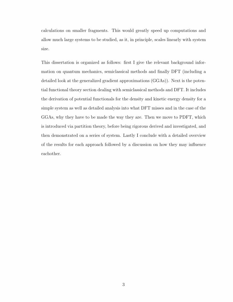
Figure 3.4: Kinetic energy densities of Fig. 3.3.
We plot results for the same potential as for Fig. 3.3, v(x) = −80 sin2(2πx). In fact,
tsemiS
is ill-behaved right at the end points, so we model its approach to the boundaries
with a simple parabola for x < 0.0875, with constant chosen to match the logarithmic
derivative at that point. The resulting integrated TS is 156.2, compared to the exact
result 157.2.
We emphasize that the correct semiclassical treatment has reduced the error in self-
consistent TF theory by a factor of 40. Thus the semiclassical approach is far more
powerful and systematic than the usual gradient expansion. How then do density
31

functionals achieve the accuracy needed for chemical and materials applications?
The answer already appears for the flat box. Inserting the exact density in T (0)
yields π2
6L2 (ζ5N3 + ζ4 9
8N2 + ζ3 3
8N), i.e. reasonably accurate quantum corrections, be-
cause most of the contribution comes from regions of not-too-rapidly varying density.
In the double-well potential, T(0)S on the exact density is only 4 times worse than
our semiclassical approximation. Thus semilocal functionals, applied to the highly
accurate densities from the KS scheme, contain typically good approximations to the
quantum corrections in the energy. In fact, for the flat box, the leading gradient
correction worsens the energy. If we alter the coefficient of TW from −1/3 to +0.424,
the corresponding ‘generalized’ gradient expansion is AE1, and far more accurate for
particles in boxes.
3.4 Including gradient terms
We can include terms of higher order in ~ in the WKB wavefunction to find gradient
corrections to the semiclassical kinetic energy formula, Eq. (3.26). Careful analysis
of this formula shows that it includes terms of order ~2. As we shall see, the next
order gradient correction to Thomas-Fermi is of order ~, hence to be a complete semi-
classical description, one must include these terms. Below I shall simply demonstrate
that using the WKB wavefunction with higher order terms and the Green’s function
methods developed above, one can recover the known gradient correction to TF[30].
However, since quantum correction terms can also be found by including these terms,
we can go further than these simple corrections. This is an obvious candidate for
future work and may shed light on the generalized gradient corrections of DFT.
32

Recall that for higher order WKB, the wavefunction is given by
φ(x) =c
√
Q(x)sin[
1
~
∫ x
dx′Q(x′)] (3.27)
where to next order
Q(x) = k(x) + ~2Q(2)(x) (3.28)
and
Q(2)(x) = +v′′(x)
4k3(x)+
5[v′(x)]2
8k5(x)(3.29)
If we now construct the Green’s function
G(x, x′;E) = −2 sin [γ1(x;E)] sin [γ2(x;E)]
~√
Q(x;E)Q(x′;E) sin [Γ(E)](3.30)
where
γ1(x;E) = γ(x;E) =1
~
∫ x
0
Q(x′′;E)dx′′ (3.31)
γ2(x;E) =1
~
∫ L
x′
Q(x′′;E)dx′′ (3.32)
Γ(E) =1
~
∫ L
0
Q(x′′;E)dx′′ (3.33)
If we first calculate the TF like term, τ1(x), TF in the sense that this gives TF to first
order and we calculate the contour integral in the same manner. As in the previous
case, we shift off the real axis and follow the contour of Fig. 3.2, then
τ1(x) = −1
4π~
∮
EF
dE[k(x;E)]2
Q(x;E)(3.34)
33

integrates to
τ1(x) =k3
F
6π~+ ~
[
v′′
8πkF
+5v′2
48πk3F
]
(3.35)
using
1
Q=
1
k− ~
2
(
v′′
4k5+
5v′2
8k7
)
+ ... (3.36)
This is exactly the gradient correction to Thomas-Fermi as calculated in Ref. [30].
3.5 Potential Scaling
Density scaling has been a particularly useful tool for the analysis and development
of DFT. A singular example is uniform coordinate scaling[27], where the coordi-
nates of a given density are linearly scaled, but normalization is preserved. This
has led to fundamental exact conditions on the exchange-correlation (XC) energy
functional[27, 32, 33, 34]. For example, the form of the local approximation to
the exchange energy can be deduced from this scaling. The adiabatic-connection
formulation[35, 36, 37, 38], much studied and used in DFT development, is essen-
tially an integral over the uniform coordinate scaling parameter[27, 39, 40]. Here, the
electron-electron interaction is scaled by a constant while the density is kept fixed,
linking the non-interacting Kohn-Sham and the fully interacting systems, and leads
to many more conditions. For example, the adiabatic connection formula is behind
rationalizing the hybrid approach[41, 42, 43, 44].
Recently, a different form of density scaling was used in the development of the PBEsol
functional[45]. Here, both the coordinate and the particle number are scaled, leading
to new insights into the XC functional. We refer to this as charge-neutral scaling[29],
34

as it is equivalent to simultaneously changing the charges on atoms and the number
of electrons, so as to keep overall neutrality.
In this section, we extend the use of density scaling as a tool in DFT. Most importantly
we introduce the concept that any form of density scaling defines a related form of
potential scaling. This leads to more exact conditions on the various DFT quantities
as functionals of densities of different particle number. Yang and others[25] have
emphasized the duality of the potential with the density, but have not related scaling
of one to the other.
Potential Scaling
Consider a density n(r) that is the ground-state density of some interacting problem
with potential vext(r). Now, introduce some positive parameter, 0 < γ < ∞, which
produces a family of densities, nγ(r), with γ defined so that γ → ∞ corresponds to
the high-density limit.
A simple example is the uniform coordinate scaling of Levy and Perdew[27]:
nγ(r) = γ3n(γr), 0 < γ <∞, (3.37)
where the prefactor was chosen to keep the density normalizd. For example, un-
der uniform coordinate scaling with γ > 1, the density of He is squeezed into a
smaller volume, and looks like a distorted version of a two-electron ion[46]. This
scaling has become a mainstay of DFT and leads to many important results. Most
importantly, when particles interact, the coordinate-scaled wavefunction is not the
ground-state wavefunction of the scaled density. Considering such a wavefunction as
a trial state in the Rayleigh-Ritz principle yields useful inequalities for the various
35

density functionals[27]:
T [nγ ] ≤ γ2 T [n], γ ≥ 1, (3.38)
Vee[nγ ] ≥ γ Vee[n], γ ≥ 1, (3.39)
and a similar condition applies for the correlation energy E [n] itself.
0 1 2 3 4r
0
1
2
3
4
5
4πr2 n(
r)
Figure 3.5: The exact radial densities of Beryllium (solid line)[47], and of the CNscaled (with ζ = 2) Helium (dashed line)[48].
A second example that we focus on here is what we call charge-neutral (CN) scaling,
in which
nζ(r) = ζ2n(ζ1/3r), 0 < ζ <∞ (3.40)
and so Nζ = ζN . We use ζ as the scaling parameter to distinguish from coordinate
scaling. This choice both scales the coordinate and changes the particle number. For
Coulomb-interacting matter, this ensures neutrality as a function of ζ. For example,
36

for single atoms, it simply implies Zζ = ζZ and the atom remains neutral. Lieb and
Simon[49] showed that Thomas-Fermi (TF) theory becomes exact for neutral atoms
as ζ → ∞, and Lieb[26] later generalized the proof to all Coulomb-interacting matter.
In Fig 1, we illustrate this scaling on the He atom density.
In both coordinate and CN scaling, as the scaling parameter is taken to ∞, the
solution simplifies. Under uniform coordinate scaling to the high-density limit, the
system becomes effectively non-interacting. Under CN scaling to the high-density
limit, Thomas-Fermi theory becomes relatively exact. In either case, we can ask how
the potential changes when the density is scaled. We define this as the potential
scaling conjugate to the given density scaling, but consider it for all values of the
scaling parameter, not just in the high-density limit.
Under coordinate scaling, in the large γ limit,
vγ(r) = γ2v(γr). (3.41)
We therefore define our potential scaling by this equation, applied for all γ. We use
a superscript to indicate that the potential has been scaled, not the density. This
is simply how the external potential would change when the density is scaled, if
the particles were non-interacting particles. For example, for a neutral atom, this
changes the nuclear charge by γ, keeping the particle number fixed. As γ → ∞, the
repulsion between electrons becomes negligible relative to the nuclear attraction, and
the density becomes that of the non-interacting limit, scaled by γ.
Similarly, under CN scaling with ζ → ∞, the TF equations become relatively exact[50],
and
vζ(r) = ζ4/3v(ζ1/3r), Nζ = ζN. (3.42)
37

Again, the conjugate potential scaling is defined by this, applied to all values of ζ.
Analogously, if self-consistent TF theory were exact, this is how the potential would
scale for any ζ as the density is scaled.
Although chosen to match the corresponding density scaling in the high-density or
high-potential limit, these potential scalings can be applied for any values of their
scaling parameter. Since scaling the potential is much more common in quantum
problems than scaling the density, often solutions are known or can be accurately
calculated for different scalings of the potential, but not of the density. In this paper,
we find relations and inequalities between such solutions that complement the ground-
breaking results of the previous generation[27].
Uniform coordinate scaling
In the old work[27], Levy and Perdew compared two different wavefunctions with the
same density, whereas we compare two different wavefunctions in the same potential.
To do this, begin from a given potential vext(r) with ground-state density n(r). Define
nγ(r) as the ground-state density of vγext(r), given by Eq. (3.41). Then nγ
1/γ(r) is a
useful trial density for the original problem. It is found by first scaling the potential,
solving the problem, and then scaling backwards to the original problem. (In Fig. 1,
the dashed line corresponds nζ(r) for the He density, with ζ = 2.) This is exactly
what was done (but with an approximate scale factor) in Ref. [46].
If nγ1/γ(r) is used as trial density for vext(r), the variational principle states that
F [nγ1/γ ] + γ−2V γ
ext[nγ ] ≥ F [n] + γ−2V γ
ext[nγ ], (3.43)
which may be rearranged as
F [nγ1/γ ] − F [n] ≥ γ−2(V γ
ext[nγ ] − V γext[n
γ]). (3.44)
38

Conversely, nγ(r) may be used as a trial density for vγext(r), yielding
Evγext
[nγ ] = F [nγ] + V γext[nγ ]
≥ F [nγ] + V γext[n
γ ], (3.45)
which can also be rearranged as
F [nγ] − F [nγ ] ≤ V γext[nγ ] − V γ
ext[nγ ]. (3.46)
Combining the two inequalities yields a constraint on the universal functional F [n]:
F [nγ1/γ ] −
F [nγ]
γ2≥ F [n] −
F [nγ]
γ2, (3.47)
which may be written in a concise form, with λ = 1/γ,
∆F λ[n1/λλ ] ≥ ∆F λ[n], (3.48)
where
∆F λ[n] = F [n] − λ2F [n1/λ]. (3.49)
Now, F [n] is typically dominated by the kinetic energy contribution, but this can be
removed, because TS[nγ ] = γ2 TS[n]. Thus
∆EλHXC
[n1/λλ ] ≥ ∆Eλ
HXC[n], (3.50)
where EHXC = U + EXC. This tells us that if we begin from, e.g., the lowest value of
Z that binds a given N electrons, then ∆EλHXC
[n1/λλ ] is an increasing function of λ.
39

Simple results can be extracted from this very general formula by taking γ to be very
large. This makes nγ(r) an essentially non-interacting density, because the external
potential dominates. Thus
n1/λλ (r) → nNI(r), λ→ 0, (3.51)
where nNI(r) is the density of the system with only an infinitesimal electron-electron
repulsion. But ∆EλHXC
[n] also simplifies as λ → 0, because all terms scale less than
quadratically. Thus
∆EλHXC
[n] → EHXC[n], λ→ 0, (3.52)
yielding the universal result that
EHXC[nNI] ≥ EHXC[n], (3.53)
applying to all potentials. For γ < 1, Eq. (3.48) is less useful, as most systems of
interest lose an electron when the external potential becomes too small. To further
simplify Eq. (3.50), we note that both the Hartree and exchange energies scale linearly
with γ, i.e.,
EHX[nγ ] = γ EHX[n], (3.54)
so that
∆EλHX
[n] = (1 − λ)EHX[n]. (3.55)
40

Table 3.1: The Hartree energies, U , for the helium iso-electronic series as calculatedwith the oep exact-exchange method as implemented in the OPMKS code[51]. Wealso demonstrate how, for two values of atomic number Z ′, the inequalities of Eq.(3.59) with γ = Z ′/Z, are satisfied. Note that if γ < 1, the inequality is reversed.The values for bordering values of Z bracket the value of U at atomic number Z andthese bounds become tighter as Z ′ increases.
Z U Z’=4 Z’=201 0.790970 3.163880 15.8194002 2.051538 4.103076 20.5153803 3.303373 4.404497 22.0224874 4.554137 4.554137 22.7706856 7.054819 4.703213 23.51606310 12.055315 4.822126 24.11063020 24.555661 4.911132 24.555661
Inserted into Eq. (3.50), we find
EHX[nγλ] + ∆′Eλ [nγ
λ] ≥ EHX[n] + ∆′Eλ[n], (3.56)
where
∆′Eλ [n] = ∆Eλ[n]/(1 − λ). (3.57)
The simplest way to test this result is by doing a Kohn-Sham calculation without any
correlation (such as oep exact exchange). Then the correlation contributions vanish
on both sides of Eq. (3.56), and so
EHX[n] ≤ EHX[nγ ]/γ ≤ EHX[nNI] (3.58)
This simplifies even further for the special case of two electrons in a spin singlet,
where EX[n] = −U [n]/2, so the inequality becomes a bound on the Hartree energy
41

Table 3.2: Hartree-exchange energies for the beryllium iso-electronic series. Valueswere also calculated with the OPMKS code with oep exact-exchange. Also shown aretwo examples of the inequalities of Eq. (3.58), again using γ = Z ′/Z. Although thequantities are more complicate that those in Table 3.1, the overall trend is the same.
Ion Z EHX Z’=10 Z’=16Be 4 4.489776 11.224440 17.959104B+ 5 6.119120 12.238240 19.581184O4+ 8 10.893545 13.616931 21.787090Ne6+ 10 14.051482 14.051482 22.482371S12+ 16 23.498356 14.686473 23.498356
Ca16+ 20 29.788628 14.894314 23.830902
alone:
U [n] ≤ U [nγ ]/γ ≤ U [nNI] (3.59)
In Table 3.1, we analyze the above inequality, Eq. (3.59), while in Fig 3.6, we plot
U [nγ ]/γ as a function of γ for exact-exchange calculations of the two-electron ion
series, beginning with H−. Indeed, the function increases toward the Bohr atom
limit of 5/4, found by inserting a doubly-occupied 1s Hydrogen atom orbital into the
Hartree energy.
To test the exchange contribution in a non-trivial way, i.e., Eq. (3.56), we repeated
the calculations for the four-electron ion series, this time beginning from Be. Again
the inequality is satisfied, and the limiting value is found by evaluating the Hartree
and exchange energies of doubly-occupied 1s and 2s Hydrogenic orbitals, as calculated
in Appendix A. These values are reported in Table 3.2 and plotted in Fig 3.7.
Lastly, we can even include extremely accurate estimates of the correlation contri-
butions for the two-electron series. We work from the data in Table I of Ref. [52].
Since the two-electron ions are generally weakly correlated, one can approximate the
scaling of their correlation energies with a Taylor-series around the high-density limit:
42

0 5 10 15 20Z,
0.8
1
1.2
U[n
γ ]/γ
Figure 3.6: Using the Hartree energies from Table 3.1, Eq. (3.59) is illustrated forγ = Z ′/Z and Z = 1. The trend is identical to that seen in Table 3.1, however it isclear that the value is approaching it’s asymptote, 5/4. This is the Hartree energyfor density consisting of the doubly occupied hydrogen 1s orbital.
EC[n] = E(0)C [n] + λE
(1)C [n] (3.60)
where E(p)C [n] are scale-invariant functionals. Since TC = −EC + ∂EC[nγ]/∂γ(γ =
1)[27], and TC is reported in their table, one can solve for these two coefficients. This
yields a value of -47.6 mH for E(0)C for He, in excellent agreement with the value of
47.9 estimated in Ref. [46], and predicts a value of -56.1 mH for H−. Using this
approximate scaling, we can insert all terms into Eq. (3.50) explicitly and find their
behavior. The numerical corrections to our previous results are negligible.
Charge-neutral Scaling
In this section, we repeat all the logic of the previous section, but apply it now to CN
scaling. After repeating similar steps (given in Appendix C), we arrive at the general
43

0 10 20 30Z,
4
5
6
EH
X[n
γ ]/γ
Figure 3.7: The Hartree-exchange energies reported in Table 3.2 are used to illustratethe inequalities of Eq. (3.58) with γ = Z ′/Z and Z = 4. Compared to Fig. 3.6, thevalue of EHX[nγ ]/γ is not as fully converged to its asymptote, however the maximumvalue of γ is 4 times smaller. The asymptotic value for this case is 586373/93312 =6.284, which is found by doubly occupying both 1s and 2s hydrogenic orbitals withZ = 4 and calculating Hartree and exchange energies.
result:
∆Fα[n1/αα ] ≥ ∆Fα[n] , (3.61)
where
∆Fα[n] = F [n] − α7/3F [n1/α] , (3.62)
and α = 1/ζ. Just as we did for coordinate scaling, we can refine our inequality sub-
stantially. By construction, ∆Fα[n] = 0 for FTF[n], so we define the useful functional:
FNT [n] = F [n] − FTF[n] (3.63)
44

as the Non-Thomas-Fermi contribution to F [n]. Our inequality then reads:
∆FNTα[n1/αα ] ≥ ∆FNTα[n] , (3.64)
where
∆FNTα[n] = FNT [n] − α7/3FNT [n1/α] . (3.65)
We find an interesting result in the limit α→ 0, if we make the reasonable assumption
that all non-Thomas-Fermi contributions scale less strongly than ζ7/3 :
FNT [nTF] ≥ FNT [n] , (3.66)
as TF becomes relatively exact in the high ζ. This inequality is fiendishly hard to test,
even in the large ζ limit. Consider, e.g., the He atom. The corresponding TF density
is well-known[53] but we would have to evaluate the exact interacting functional on
it to find the non-TF contribution. All the above results also apply directly to non-
interacting electrons in a potential, such as the Bohr atom[54], with F replaced by TS,
and the TF contributions calculated with no Hartree term. But the same difficulties
remain.
There is one case where we know enough already to test. For the hydrogen atom (or
any one-electron system), F = T only, and is given by the von Weizacker functional.
The TF density (with or without interaction) is well-known and singular at the origin,
making the von Weizacker energy diverge. Thus, the formula is satisfied, but not very
informative.
Lastly, we consider Thomas-Fermi-Dirac-Weizsaker theory[23] (TFDW). Here we add
45
to TF the local exchange
E(0)X [n] = AX
∫
d3r n4/3(r), (3.67)
where AX = −(3/4)(3/π)1/3, and the next order gradient correction to the kinetic
energy,
T(2)S [n] =
1
72
∫
d3r|∇n(r)|2
n(r). (3.68)
Both these terms scale the same way under CN density scaling, i.e.,
F (2)[nζ ] = T (2)[nζ ] + E(0)X [nζ ] = ζ5/3(T (2)[n] + E
(0)X [n]). (3.69)
Then can write the inequality as
F (2)[nζ ] ≥ ζ5/3F (2)[n], (3.70)
where n(r) has been evaluated self-consistently within TFDW and ζ ≥ 1. Thus
F (2)[nTF] ≥ F (2)[nζ ]/ζ5/3 ≥ F (2)[n], (3.71)
where nTF(r) is the Thomas-Fermi solution for the same potential as for n(r).
Conclusion
Potential scaling, conjugate to a given density scaling, promises to be a useful tool
in density functional theory. It leads to many exact conditions that can be used in
functional construction. We have applied it to two distinct types of scaling: uniform
coordinate scaling and charge neutral scaling. In both cases, we have found sev-
eral interesting bounds. Uniform coordinate scaling was useful for analyzing Kohn-
46

Sham DFT, leading to inequalities involving the only unknown in DFT, the exchange-
correlation functional. The limit of this inequality involves evaluating the Hartree-
exchange-correlation energy of the density of non-interacting fermions in the external
potential. This connection between the interacting and non-interacting systems res-
onates with standard approaches in many-body perturbation theory. We illustrate
the bounds on the Hartree-exchange energy this inequality provides by performing
OEP exact exchange calculations on helium and beryllium, showing the approach
to their asymptote. On the other hand, charge-neutral scaling provides inequalities
involving Thomas-Fermi quantities. The Thomas-Fermi approximation becomes rel-
atively exact for all electronic systems[49, 26] and these relations link the corrections
to Thomas-Fermi with the true system, including those of TFDW theory. However
evaluating the TF density within these theories often leads to divergences[55, 56].
In the derivation of these inequalities, the variational principle was used to link the
unscaled and scaled systems. If we now use an approximate functional and use its
self-consistent densities, the inequalities are automatically satisfied if the previous
scaling relationships are true. This makes it more difficult to use these inequalities
as exact conditions for functional construction, however work is ongoing to interprete
the effect of these inequalities on potential functionals, like those of Ref. [25].
We thank Eberhard Engel for use of the OPMKS code and also thank Cyrus Umrigar
for providing exact densities.
3.6 B88 Derivation
As discussed in chapter 2.4.1, the natural successor to LDA is a semi-local (or
gradient-corrected) approximation which adds information about the derivative of
the density at that point. In fact, in the same paper in which LDA is introduced, so
47

too is the gradient expansion approximation (GEA) for XC. The coefficients of the
GEA are determined by the energy of a slowly-varying gas[13, 14, 57]. However it
was found that the GEA often worsened LDA results and two decades passed before
substantial improvements were made.
Generalized gradient approximations (GGAs) effectively resum the gradient expan-
sion, but using only |∇n|. The B88 functional[9] is the most used GGA for exchange
overall (as part of B3LYP[10, 58]), but the most popular GGA in solid state appli-
cations is PBE[8]. Neither reduces to the GEA in the limit of small gradients. In
this paper we explain the reason why this must be the case. Asymptotic expressions
for the energy components as functionals of N , the number of electrons, display ‘un-
reasonable accuracy’[59] even for low N . In order to give good energies for finite
systems, any approximate XC functional must have accurate coefficients in its large-
N expansion. LDA gives the dominant contribution, but the GEA does not yield an
accurate leading correction for atoms. Popular GGAs such as B88 and PBE do get
this correction right.
In Ref. [29], the underlying ideas behind this work were developed, however the rea-
soning was based upon scaling the density and not on the potential scaling discussed
below. We refine these ideas and explicitly show how they can be used for functional
development, and in particular we show how the parameter in B88 may be derived in
a non-empirical manner.
Asymptotic expansion in N Begin with any system (atom, molecule, cluster, or
solid) containing N electrons. We then imagine changing the number of electrons to
N ′. Since we usually begin from a neutral system, usually we consider only N ′ > N .
Thus we define a scaling parameter ζ = N ′/N > 1. As we change the particle
number, we simultaneously change the one-body potential vext(r) as in Eq. (3.1) so
as to retain overall charge neutrality. We refer to this as charge-neutral (CN) scaling.
48

For an isolated atom, Z → ζZ under this scaling, so it remains neutral as the electron
number grows. For molecules with nuclear positions Rα and charges Zα, Zα → ζZα
and Rα → ζ−1/3Rα. In the special case of neutral atoms, the resulting series for the
energy is well-known:
E = −a0N7/3 − a1N
2 − a2N5/3 − ... (3.72)
where a0 = 0.768745, a1 = −1/2, and a2 = 0.269900 [59, 60]. We say an approxima-
tion is large-N asymptotically exact to the p-th degree (AEp) if it recovers exactly
the first p+1 coefficients for a given quantity under the potential scaling of Eq. (3.1).
Lieb and Simon[49, 26] showed that Thomas-Fermi (TF) theory becomes exact in the
limit ζ → ∞ for all systems. TF is exact in a statistical sense, in that TF gives the
correct first term of Eq. (3.72), but not the other terms. We say TF is AE0 for the
total energy.
A similar expression exists for the exchange component of the energy alone:
EX = −c0N5/3 − c1N − ... (3.73)
where c0 = 0.2208 = 9a2/11 and c1 will be the main topic of this paper. In a
similar fashion, Schwinger demonstrated that the local approximation for exchange
is AE0, and this coefficient is given exactly by local exchange evaluated on the TF
density[59, 60, 50]. However in order to give atomic exchange energies needed for
chemical accuracy, any exchange approximation should be at least AE1.
Now suppose we want to make a local approximation for EX but know nothing about
the uniform gas. Dimensional analysis (coordinate scaling[27]) tells us that it must
49

be of the form:
ELDAX
[n] = AXI, I =
∫
d3r n4/3(r). (3.74)
Requiring that this gives the leading contribution to Eq. (3.73) then fixes the value
of the constant AX. Using any (all-electron) Hartree-Fock atomic code, such as were
already available in the 1960’s[61], one calculates I for densities running down a
particular column of the periodic table and then deduces its dependence on Z5/3.
A modern alternative is to use the fully numerical OPMKS code[51] using the OEP
exact exchange functional to find densities for neutral atoms from Z = 1 to Z = 88.
By fitting, one finds I = 0.2965Z5/3 and hence AX = −0.7446. This is remarkably
close to the derived result of
AX = −3
4
[
3
π
]1/3
= −0.7386. (3.75)
Thus, without any recourse to the uniform electron gas, we have derived the correct
local approximation to EX[n].
This demonstrates that, via asymptotic exactness, the local approximation to ex-
change is a universal feature of all systems as N → ∞, when scaled appropriately.
(In fact, Schwinger only proved this for atoms[59], we know of no proof for arbitrary
systems).
Theory
LDA yields the dominant term in either the asymptotic charge-neutral expansion
(ζ → ∞) or the gradient expansion for the slowly-varying electron gas, s → 0. We
next show that, contrary to popular myth, the important expansion is the charge-
neutral expansion, not the gradient expansion.
50

0 0.2 0.4 0.6 0.8 1
Z-1/3
-0.4
-0.35
-0.3
-0.25
-0.2
Ex /
Z5/
3-0.2208
Figure 3.8: The OEP exact exchange energies EX for neutral atoms from Z = 1 to 88,divided by Z5/3 in order to pick out the leading term in its asymptotic series. Theleading corrections are proportional to powers of Z−1/3. The values for the noble gasatoms are given as the circle symbols.
The charge-neutral expansion can be applied to any type of matter, be it molecule
or extended solid. For any finite system, the density decays exponentially far from
the nuclei. This is a key distinction between finite systems and bulk matter, treated
with periodic boundary conditions. Bulk matter has no such regions.
But, for slowly-varying gases, or more generally when there are no classical turning
points at the Fermi surface, the charge-neutral scaling and the gradient expansion
become identical, i.e., the gradient expansion for the slowly-varying gas is simply a
special case of charge-neutral scaling. To see that this is so, consider just the kinetic
energy as a density-functional. Here the gradient expansion is known out to 6th
order[55], and eventually the integrated quantity itself diverges for atomic densities,
due to the evanescent tail. But no such divergence occurs for extended systems with
finite density everywhere[55, 56].
Thus CN scaling applies to all systems, but only becomes identical to the gradient
expansion for slowly-varying bulk systems. For the dominant contribution, effectively
the local Fermi wavelength becomes short on the length scale on which the density is
51

0 0.2 0.4 0.6 0.8 1
Z-1/3
-0.35
-0.3
-0.25
-0.2
Ex /
Z5/
3-0.2208
Figure 3.9: We add to Fig. 3.8 the results for the LDA functional evaluated on theOEP densities (dashed-line) keeping the XX values (solid line). As in Fig. 3.8, theNoble gas atom are highlighted with circle and square symbols for XX and LDArespectively.
changing, so that the local approximation applies, and yields the exact answer for this
term. Hence LDA reproduces the AE0 terms, but GEA does not produce the leading
corrections. All this has been amply demonstrated for simple 1d model systems[50],
and for the Kohn-Sham kinetic energy for atoms[62].
Here we apply the same reasoning for exchange. The local approximation becomes
relatively exact as ζ → ∞, but the gradient expansion does not reproduce the leading
correction in the CN expansion. Below, we use the simple reasoning of Ref. [29] to
recover this leading correction. We perform a much more extensive calculation of the
asymptotic behavior, using methods developed in Ref. [62]. We find, in agreement
with Ref. [29], that the leading correction for atoms is about double that given by
the gradient expansion, matching quite closely that of B88 and of PBE. Reversing
this logic for B88, we show that B88 may be more or less derived non-empirically via
the constraint that the approximation be AE1. If we enforce AE1 exactly, we find a
slightly different value for β, and discuss the properties of the resulting functional,
excogitated B88.
52

0 0.2 0.4 0.6
Z-1/3
-0.25
-0.2
-0.15
-0.1
-0.05
(EX
X -
ExL
DA
) / Z
Figure 3.10: We now find the next coefficient in the exchange asymptotic series.To minimize the error due to shell structure oscillations, the LDA exchange energyis subtracted from the exact exchange for each atom. As both give the leadingcorrection, their difference will then have ∆cZ, ∆c = c1 − cLDA
1 , as the leading termin its asymptotic expansion, . The dashed line is the result of fitting to the noble gasatoms (circle symbols).
Extracting asymptotic coefficients
Under the potential scaling of Eq. (3.1), any approximation for the exchange energy
that reduces to LDA in the uniform limit has an expansion in N like Eq. (3.73),
with the same value for c0. However the coefficient c1 depends on the particular
approximation. Below we explain the procedure used to extract these coefficients.
As mentioned in the previous section, the OPMKS[51] electronic structure code is a
fully numerical electronic structure code that has the ability to perform optimized
effective potential (OEP) calculations. We evaluate the various approximations using
atomic densities found with the OEP exact exchange (XX) method. The densities
found using this method will be extremely close to the exact densities despite the
fact that correlation is missing. Moreover the effect of correlation will contribute at
higher orders in the asymptotic expansions of the energy than those we are interested
in. Thus EXX calculations are in principle sufficient for extracting the coefficient we
53

0 20 40 60 80Z
-20
-15
-10
-5
0
5
EX
- c
0Z5/
3
Figure 3.11: In order to see that LDA does not significantly contribute to the higherorders of the exchange asymptotic series, we plot the difference between LDA andthe leading term c0Z
5/3 (dashed line), as a function of Z. The exact exchange valueis also shown (solid line).
seek.
In Fig. 3.8, we plot EX/Z5/3 vs Z−1/3 where EX is the exchange energy from the
exact exchange calculation. Since the leading term in the asymptotic expansion of
Eq. (3.73) is Z5/3, this procedure picks out the c0 coefficient as a constant while
all other terms are functions of Z−1/3. One can see that the curve in Fig. 3.8 is
heading towards the exact value of c0 = −0.2208, but it is difficult to extract higher
coefficients due to oscillation of the curve due to the shell structure.
To overcome this difficulty, in Fig.3.9 we add the LDA curve to Fig.3.8. It can be seen
that it too recovers the exact c0 coefficient, but also clearly differs in higher orders
in the asymptotic expansion. More usefully, we see that the LDA curve mimics the
oscillations shown by exact exchange, so subtracting LDA from EXX will minimize
this effect and make the extraction of asymptotic coefficients more accurate.
In Fig. 3.10, we plot (EX − ELDAX
)/Z vs Z−1/3 and find that it behaves close to
linearly. There appears to be no Z4/3 term in EX. Such a contribution was argued
54

0 0.2 0.4 0.6
Z-1/3
-0.125
-0.1
-0.075
-0.05
EX
(2) /
Z
Figure 3.12: We use the same procedure as in Fig. 3.10 to find the ∆c coefficient forthe gradient correction to LDA, E
(2)X [n], as defined in Eq. (2.49). The dashed line
was fitted to the noble gas atoms (circle symbols).
not to exist in Ref. [29], but this was based on CN scaling of the density and studying
the behavior of the terms in the gradient expansion. That reasoning is insufficient, as
the expansion should be performed in terms of the potential, as described in Sec. 3.6.
But since the Scott correction (the Z2 contribution to the total energy) comes from
the core region, there is no reason to expect an analogous contribution for exchange.
In order to show this and also to precisely determine the c1 coefficient, one should use
the techniques developed by Schwinger for deriving the Scott correction to the total
energy[59], but apply them to exchange.
To further reduce the remaining uncertainty due to shell structure oscillations, we
choose simply to use the noble gas atoms (excluding helium) for our fit. The strongest
deviations from linearity come from the transition metals and lanthanides and ac-
tinides. We fit the difference (EX − ELDAX
)/Z with a straight line in Z−1/3, and
extrapolate to Z → ∞, finding ∆c = −0.2240, where ∆c = c1 − cLDA1 , and
EX ≈ ELDAX
− 0.2240Z + 0.2467Z2/3. (3.76)
55

The coefficient of the last term is given by the slope of the dashed line in Fig. 3.10,
although the meaning of this term is unclear in the presence of such strong oscillating
contributions.
0 20 40 60 80Z
-0.8
-0.4
0
0.4
0.8
%E
rror
of
( E
X
LD
A -
0.2
240
Z +
0.2
467
Z2/
3 )
Figure 3.13: The percentage error of the approximate asymptotic series given in Eq.(3.76) is plotted as a function of Z. The error is remarkably low and demonstratesthe power of these asymptotic series.
If instead we used the alkaline earth atoms (excluding beryllium), we find an almost
identical value, ∆c = −0.2236. If we use all elements with Z > 10, we find a
similar value, ∆c = −0.2164. If all elements from Z = 1 to 88 are used, we find
∆c = −0.1982. In Ref. [29], ∆c was found using noble gas atoms, except with
the helium value included, and that method gave a value of ∆c = −0.1978. In our
analysis, atoms with Z < 10 are not used as they are not necessarily dominated by
the asymptotic series.
Since LDA displays the shell oscillations that prevented us from fitting EXX directly,
the value of the LDA c1 coefficient cannot be found exactly. But we estimate 0 ≥
cLDA1 ≥ −0.04, i.e., at least five times smaller in magnitude than ∆c. In Fig 3.11,
we show EX − c0 Z5/3 as a function of Z for both the exact values and within LDA,
demonstrating that the linear contribution comes almost entirely from the beyond-
LDA terms.
56

Finally we determine ∆c for GEA. In Fig. 3.12, we plot (EGEAX
− ELDAX
)/Z vs Z−1/3
in order to find ∆c = cGEA1 − cLDA
1 , finding ∆c = −0.1062. This plot is much closer
to linear than the previous one. The leading corrections to LDA in the asymptotic
expansion produce corrections to the shell structure beyond those captured by LDA
evaluated on the exact density [50, 62]. Although the smooth contribution can be
partially captured by GEA, there is almost no correction to the shell structure. Just
as for the kinetic energy[62], GEA yields a correction to the smooth part that is about
half of the accurate value.
20 40 60 80Z
-10
-5
0
5
10
100
× (E
XX
- E
X
appr
ox )
/ E
XX
LDAGEAMGEA
Figure 3.14: The percentage error for LDA, GEA and the modified GEA (MGEA)
exchange functionals for Z > 10. The coefficient of E(2)X is multiplied by 2.109 in
order to make the MGEA AE1 asymptotically exact.
To understand the power of these asymptotic expansions, we add the corrections of
Eq. (3.76) to the LDA energies, and in Fig. 3.13 plot the percentage error relative to
exact exchange, as a function of Z. For all but the second row of the periodic table,
the resulting error is below 0.5% in magnitude, and typically of order 0.2%.
Generalized gradient approximations
Generalized gradient expansions were designed to improve energetics over LDA for
electron systems of interest and relevance. Early versions, such as PW91[63, 64], were
57

Table 3.3: ∆c = c1 − cLDA1 values for several different functionals.
EX LDA GEA B88 PBE∆c −0.2240 - −0.1062 −0.2216 −0.1946
tortured into reducing to the gradient expansion when the density is slowly varying.
But this was later given up, in both B88 and PBE exchange, which both reduce to the
gradient expansion form for slow variations, but with coefficients much larger than
that of the gradient expansion.
Our analysis explains why this must be so. Regardless of its derivation, any modern
GGA for exchange is tested against the neutral atoms. Any approximation that
cannot recover the right c1 will be generally inaccurate for these energies, and so
discarded. Thus any that become popular have already passed this test.
20 40 60 80Z
-1
-0.5
0
0.5
1
100
× (E
XX
- E
X
appr
ox )
/ E
XX
MGEAB88PBEExcogitated B88
Figure 3.15: We add to Fig. 3.14 the results for B88, PBE, and the excogitated B88functional, all evaluated on the OEP exact exchange densities.
In Table 3.3, we give the results for ∆c for several different functionals. The same
methodology was used in all extractions. Both popular GGA’s recover (at least
approximately) the accurate value. B88, designed specifically for molecular systems, is
very close to the accurate value. PBE exchange is less so, but is also designed to bridge
molecular and solid-state systems. The PBE value is between that of GEA and B88,
58

but much closer to the latter than the former. Taking advantage of this insight, a new
variation on PBE, called PBEsol[45], restores the original gradient expansion, thereby
worsening atomization energies (total energy differences), but improving many lattice
constants of solids over PBE and LDA.
Deriving the β in B88
The exchange energies found using GGAs such as B88 or PBE are generally dominated
by their gradient expansion components for most chemically relevant densities. Thus,
to make B88 AE1, it is sufficient to impose this exact condition on just the E(2)X [n]
functional form. Since both B88 and the GEA are built on top of LDA, we can simple
look at the ∆c values calculated above. If we set µ = 2.109µAK in Eq. (2.49), we
multiply the c1 coefficient of GEA by a factor of 2.109, making it AE1. In Fig. 3.14,
we name this functional MGEA for modified GEA and plot its percentage errors. The
values for LDA and GEA are also shown. It can be seen that modifying GEA to be
AE1 has greatly reduced the error.
We now require that the B88 functional form, Eq. (2.52), reduce to this MGEA for
small values of x. Using Eq. (2.51), this corresponds to using a value of β = 0.0050.
Thus we have derived an excogitated B88 that is free of any empirical parameters.
The actual value used in B88 is βB88 = 0.0053 (for spin-polarized systems this becomes
0.0042, which is the value given in Ref. ([9])), so the values are very close. This is
not surprising as fitting to Hartree-Fock exchange energies is an approximate way
of demanding asymptotic exactness. Interestingly, the value quoted as the high-Z
asymptote in Ref. [9] and found using Ref. [15] is essentially the same as our value,
but was evidently rejected in favor of a better fit. In Fig. 3.15, we plot the percentage
errors for B88, PBE, and the excogitated B88. As is typical for empirically-fitted
functionals, B88 performs very well for systems close to the data set used in the fitted
procedure. Although the error for PBE is higher than both B88 and the excogitated
59

B88, it is systematic in its overestimation. As noted, PBE was designed to perform
reasonably well for a wide range of systems, so again its behavior is not surprising. On
this data set, the excogitated B88 was never going to do better than B88, although
it remains to be seen how it performs for more complicated systems.
conclusion
We have carefully and systematically extracted the leading large-Z correction to the
exchange energy of atoms. Our results differ slightly from those of Ref. [29] but yield
the same qualitative conclusion, i.e., that the gradient expansion yields an error of
a factor of 2 or more for this coefficient. We have clarified some of the reasoning,
and applied it more generally to any atom, molecule, or cluster. By looking in detail
at the exchange energy asymptotic series for neutral atoms, we have demonstrated
the power of using such series for functional development. Requiring that the small
gradient expansion of B88 capture the two leading coefficients of the asymptotic
expansion is a method by which the unknown coefficient β can be found. This gives
a coefficient very close to the one actually used in B88 and thus is an ex post facto
‘derivation’ of B88. Inserting our most accurate estimate for β into the B88 form
yields an excogitated B88.
We thank Eberhard Engel for the use of his atomic OPMKS code, and NSF CHE-
0809859 .
3.7 Implications for DFT
So what does this mean for modern electronic structure theory? Most importantly,
this work unites rigorous proofs about TF theory[26], Schwinger’s semiclassical results
for neutral atoms[22], and modern functional development for KS calculations.
60

Exchange: We have shown that the local approximation to exchange becomes exact
as ζ → ∞ for all systems, consistent with the fact that all popular functionals recover
this limit. Furthermore, to be AE1 for EX of atoms, their small gradient limit must
be about double that of the gradient expansion[29], and this is also true for both
empirical[9] and non-empirical functionals[8]. These functionals agree for moderate
gradients, and differ for large gradients. For periodic systems without turning points,
the gradient expansion is AE to the order of the gradients. Restoring the original gra-
dient expansion greatly improves lattice parameters[24]. Finally, recent beyond-GGA
functionals that recover the 4th-order gradient expansion yield good approximations
for the enhanced gradient coefficient in atoms[29].
To apply the methods developed here directly to atoms, we need to generalize them
to include turning points, evanescent regions, and Coulomb cores. Such a scheme
might produce a derivation of an GGA beyond the small gradient limit.
Correlation: As the behavior ofEC is not governed by a simple asymptotic expansion[29],
we have not found a universal limit in which local correlation becomes exact. Con-
sistent with this, most non-empirical EC functionals are designed to be exact when
the density is uniform[8], but this condition is violated by empirical functionals[10].
Now EXC for a large jellium cluster is dominated by a bulk contribution (exact in
LDA), and a surface contribution, which can be accurately approximated by a GGA.
Restoring the density-gradient expansion for EX in PBE yields a highly accurate
surface exchange energy, so the analog is to recover the surface correlation energy[24].
KS kinetic energy: A holy grail for many years[65] has been to find an accurate
kinetic energy functional, TS[n], bypassing the construction of KS orbitals. Almost all
approaches begin from a semilocal expression, sometimes enhanced by non-locality
based on linear response. This study shows that, if one is interested in total energies,
61

a vital feature is to be asymptotically correct for neutral atoms. Thus, as ζ → ∞ in
either potential- or density-scaling, the functional must reduce to TF. For atoms, the
gradient expansion of TS[n] works rather well. The coefficient of Z2 is -0.65 in TF
theory, -0.53 if T (2) is included, and -0.52 if T (4) is added [53]. Thus each succesive
term in the gradient expansion brings it closer to being AE1, since the exact value is
-1/2. Generalizing the gradient expansion to make it AE2 produces a more accurate
functional for total energies of both atoms and molecules[53]. Lastly, our example
here shows how much simpler the kinetic energy is as a functional of the potential
than of the density.
62

Chapter 4
Partition Density Functional
Theory
In the world of electronic structure, molecules and solids are typically considered in
one of two distinct ways. In the first, the system is treated as a whole and molecular
orbitals (or bloch wavefunctions for bulk solids) are calculated. These are solutions
of some effective potential theory, such as Kohn-Sham[1, 2] density functional theory
or Hartree-Fock[66, 67], and often describe well the system near equilibrium geome-
tries. The major difficulty is then finding usefully accurate approximations to the
total energy. In the second view, one considers isolated atoms as the starting point,
and then weak interactions between such units. This view appears necessary for
strongly-correlated solids such as NiO, strongly-correlated molecules such as Cr2, or
any molecule as its bonds are stretched. In such cases, standard approximations for
the single-reference approach usually fail, often quite completely. Thus the worlds of
weak- and strong-correlation have practically divided[68].
In this work, we show that the partition theory of Ref. [69] plays a role analogous to
63

that of the Kohn-Sham formalism in density functional theory (DFT). In Kohn-Sham
theory[2], a reference system is created which is much easier to solve and in which
the interactions between electrons have been turned off. In partition theory[69, 70],
the reference system has been constructed from effective isolated fragments (e.g.,
atoms) between which there are no interactions. In both theories, the total electronic
density of the system is used as the connection between reference and reality: it
remains unchanged from one to the other, and so uniquely defines the reference.
Many other analogies are made within the paper. Suffice to say that, just as KS DFT
is particularly well-suited to weakly-correlated systems, partition theory works best
for weakly interacting fragments.
I start with the relevant background information on partition theory. Following this,
density functional partition theory (PDFT) is formally introduced, before being ana-
lyzed in detail. Next I illustration PDFT on three different systems, each highlighting
a feature of PDFT. The point of these illustrations is to show that PDFT is an ex-
act theory and will provide the exact molecular energy and molecular density at
self-consistency.The first system studied is a homonuclear diatomic molecule. This
system is also used to demonstrate partition theory, so we can see the PDFT converge
to the PT results. Next we move to the more complecated case of a heteronuclear
diatomic molecule, which creates non-symmetric charges on the two atoms. In both
of these examples, neutral diatomic molecules are used as the kinetic energy density
functional is known analytically for two or less fermions, in the final example I study
a 12 atom, 12 fermion chain. This example is much more complicated, but is still
solved exactly.
64

Figure 4.1: Two examples of binary fragmentation into fragments A and B. The figureon the left shows a hydrogen molecule at equilibrium bond length, while on the right,an ethene molecule is shown with one substituent cornered off as a fragment.
4.1 Partition Theory
Partition theory[69] provides a method for breaking a system into a sum of fragments.
Begin from the one-body potential, v(r), which is typically a sum of contributions,
most from individual nuclei; e.g.
v(r) = −∑
β
Zβ
|r − Rβ|, (4.1)
where Zβ is the atomic charge of a nucleus at point Rβ. In partition theory, we group
these contributions into Nf fragments of our choosing:
v(r) =
Nf∑
α=1
vα(r) , (4.2)
and each vα(r) is the sum over one or more nuclei. The simplest possible choice is to
divide the system into two parts (Nf=2), which we call binary fragmentation. These
parts would obviously be the two nuclei in a diatomic molecule, but could also be the
nuclei of a chemical group extracted from a large molecule, or those of a molecule
interacting with a surface. One can imagine many examples that could prove useful,
examples of which can be seen in Fig. 4.1. An alternative choice is atomization,
in which every term in Eq. (4.1) above is separated, and the number of fragments
matches the number of nuclei.
65

Once the fragments have been picked, the partition problem is to find fragment den-
sities nα(r) such that they add to the total molecular density:
Nf∑
α=1
nα(r) = n(r) . (4.3)
Within partition theory, this is done by minimizing the total energy of the frag-
ments, Ef , with the constraint that the sum of the fragment densities must match
the molecular density, i.e. Eq. (4.3). The total energy of the fragments is
Ef =
Nf∑
α=1
ǫα , (4.4)
where ǫα is the energy of each fragment. Since there is no constraint that a fragment’s
particle number, Nα, be an integer, the PPLB formulation[71, 72] is used. Thus
ǫα = (1 − να)Eα[npα] + ναEα[npα+1] (4.5)
and
nα(r) = (1 − να)npα+ ναnpα+1 (4.6)
where
Eα[n] = F [n] + Vα[n] = F [n] +
∫
d3r n(r) vα(r) (4.7)
is the energy density functional for each fragment α. The fragment particle number
is Nα = pα + να, pα and pα + 1 are the lower and upper bordering integers of Nα and
0 ≤ να < 1. The PPLB scheme is simply that of the fragment in contact with an
infinite but distant reservoir.
66

Figure 4.2: Top panel: The exact density (solid line) for two non-interacting fermionsin the potential defined in Eq. (4.19) with R = 3 and shown below. The two exactpartition densities (dotted lines) for this system. Bottom panel: The correspondingmolecular potential (solid line) as defined in Eq. (4.19).
We note the following:
• if all fragments are separated from each other, these fragment densities become
exactly those of the isolated fragments, n(0)α (r).
• One solves the Hamiltonian for each isolated fragment independently of the
other fragments. It is the sum of these fragment energies that is minimized.
• In principle finding the minimum requires first solving for the molecular density,
and so is even more work than solving the initial problem. But an exactly
analogous statement can be made about KS DFT.
The process of finding the minimum produces an extremely useful conceptual tool.
67

Minimizing the Lagrangian:
G = Ef − µ
Nf∑
α=1
∫
d3r nα(r) −N
+
∫
d3r vp(r)
Nf∑
α=1
nα(r) − n(r)
(4.8)
yields the solution to the partition problem[69]. The Lagrange multiplier µ is iden-
tified as the chemical potential, while the Lagrange multiplier that constrains the
sum of the fragment densities to be the molecular density is a potential, dubbed the
partition potential, vp(r). This is a global property of the molecule, uniquely defined
once we have chosen a particular fragmentation. It has the interesting aspect that,
when added to any fragment potential, the sum is exactly that potential for which the
fragment density is a ground state density. In the upper panel of Fig. 4.2, the exact
total density for a model system is shown. It is the solution for two non-interacting
fermions in the potential shown in the lower panel of Fig. 4.2 and is discussed in
detail in Sec. 4.3. Solving the partition problem yields the two fragment densities,
which are also shown in the upper panel of Fig. 4.2. It can be seen that adding these
two fragments densities will give the total density. In the lower panel of Fig. 4.3,
we show the exact partition potential for this problem. When added to a fragment
potential, it gives an effective potential for each fragment, this is shown as the dotted
line in the lower panel of Fig. 4.3. The ground-state density of this effective potential
can be seen in the upper panel of Fig. 4.3, it is exactly the same as the fragment
density shown in the upper panel of Fig. 4.2.
We emphasize here that once a choice of fragmentation has been made, the entire
procedure is then unambiguously defined, and leads to unique fragments. The user
chooses fragments depending on which aspects they wish to study, usually guided by
chemical intuition.
68

Figure 4.3: Top panel: The fragment density (dotted line) for the B atom of Fig.4.1. Bottom panel: The exact partition potential vp(x) (solid line) for this system,the nuclear potential vB(x) (dotted line), and the fragment potential vB(x) + vp(x)(dashed line). This potential has the fragment density shown in the upper panel asits ground state density.
4.2 Partition density functional theory
In this section, we develop a methodology which allows one to calculate a molecular
density and energy from individual calculations on fragments, via a self-consistent
loop. In this sense, it is the analog of the KS method, in which the energy is found from
self-consistent calculations on non-interacting electrons. Clearly such a capability in
general could have tremendous significance for many areas of current research, from
O(N) scaling to QM/MM methods.
To do so, think of the total fragment energy, Eq. (4.4), as analogous to the KS energy
of Eq. (2.39). Then define the partition energy as
Ep = E − Ef , (4.9)
69

analogous to Eq. (2.40), the Hartree-XC energy in KS theory. If E0f =
∑
α ǫ0α is the
total energy of the isolated fragments, then we can write
Ep = Edis + Erel, (4.10)
where Erel is the fragment relaxation energy:
Erel = E0f − Ef (4.11)
and Edis = E − E0f , is the dissociation energy. For any bound molecule, Edis < 0.
Furthermore, since E0f is the ground state energy for the isolated fragments system,
Ef > E0f . Thus Ep < 0 and is expected to be much smaller than the total energy (on
the scale of chemical bonding), and vanishes as the fragments are pulled apart.
We can consider the partition energy as a functional, Ep[{nα}], of the fragment den-
sities alone, for the given external potential and choice of fragmentation. Now, we
examine the effect of making small variations in one fragment density, δnα(r), to the
partition energy. The first term of Eq. (4.9) is the ground-state energy of the sys-
tem, so variations in the density are zero, because we are at its minimum. For Ef ,
the second term, only the α-th fragment energy changes. Since the fragment density
minimizes the α-th fragment in the presence of vp(r), then vp(r) = δǫα/δnα(r), so
that
vp(r) =δEp[{nα}]
δnα(r), (4.12)
i.e., given any expression for Ep[{nα}], we can extract the corresponding partition
potential, vp(r), and then calculate new fragment densities, which are then used to
generate a new partition potential, and so on. Thus approximating Ep[{nα}] produces
a closed loop, and a direct scheme for doing a PDFT calculation. The steps of a PDFT
70

calculation are:
1. Guess the fragment densities {nα}. A reasonable guess would be {n0α(r)}, the
densities of the isolated fragments.
2. The fragment charges, {Nα} , are determined by the fragment chemical poten-
tials.
3. Construct the partition potential, vp(r), using Eq. (4.12).
4. Solve for each nα(r) in its respective fragment potential vα(r) + vp(r).
5. Cycle steps 2, 3 and 4 until self-consistency.
6. Along with the fragment densities, this yields the total molecular density and
the molecular energy (via E = Ef + Ep).
In principle, any electronic structure method can be used to calculate the fragments.
However, in practice, most of such methods will not provide a way to functionally
differentiate the corresponding Ep. Even within KS DFT, one does not usually know
the non-interacting kinetic energy, TS, as a functional of the density. Only with an
explicit density functional can the corresponding derivative needed for the partition
potential be taken.
To derive an expression for vp(r), we write Ep[n] in terms of DFT quantities:
Ep[n] = F [n] −
Nf∑
α=1
F [nα] +
Nf∑
α=1
Nf∑
β 6=α
∫
nα(r)vβ(r). (4.13)
For simplicity, we assume Nα is an integer, otherwise Eq. (4.5) must be used. so we
can write the partition potential in terms of functional derivatives of the universal
71

functional:
vp(r) =δF [n]
δn(r)−δF [nα]
δnα(r)+
Nf∑
β 6=α
vβ(r) . (4.14)
This gives an expression for vp(r) for each of the Nf fragments. Using the fact that
the universal function can be decomposed into F [n] = TS[n] + U [n] + EXC[n], this
leads to
vp[{nα}](r) =δTS[n]
δn(r)−δTS[nα]
δnα(r)+vXC[n](r)−vXC[nα](r)+
Nf∑
β 6=α
(vβ(r) + vH[nβ](r)) (4.15)
for any α, and using the fact that the Hartree potential is linear in n(r). Explicit
density functional expressions are needed for both TS[n] and EXC[n]. However since
the expression only depends on differences between the functional derivatives of these,
some of the error due to approximating these may cancel.
To find the fragment occupations, note that at self-consistency, the chemical poten-
tials of all the fragments will be equal. We choose N(k+1)α = N
(k)α − Γ
(
µ(k)α − µ(k)
)
,
where Γ is another positive constant and µ is the average of the fragment chemical
potentials, used in conjunction with Eq. (4.5) for the functionals.
If we use DFT to perform the fragment calculation, the KS potential for the α-th
fragment is found from Eq. (4.12) in KS quantities:
vS,f,α[nα, nα](r) = vS[nα](r) + (v(r) + vHXC[n](r) − vS[n](r)) , (4.16)
where vS[n](r) = −δTS[n]/δn(r), and n(r) = nα(r) + nα(r). This is the central result
of this paper, as it gives the fragment KS potential for a pair of trial densities, nα(r)
and nα(r), in terms of quantities from KS-DFT.
72

4.3 Homonuclear Diatomic Molecule
For one or two electron systems, the kinetic energy density functional is given exactly
by the von Weizsacker functional:
TW[n] =1
8
∫
d3r|∇n(r)|2
n(r), (4.17)
and if we study non-interacting fermions, then Ep[n] as a density functional is known
exactly. Taking the functional derivative with respect to a fragment density yields
the partition potential, which for a binary fragmentation of a symmetric system is:
vp(r) = vB(r) +
(
n′2(r)
8n2(r)−n′′(r)
4n(r)
)
−
(
n′2A(r)
8n2A(r)
−n′′
A(r)
4nA(r)
)
(4.18)
in the absence of electron interaction. For a non-symmetric system, the general
formalism[71] for non-integer particle number must be used. If we work in one di-
mension, then the 1-fermion fragments can be solved easily.
For this example, we use a 1/ cosh2(x) potential for the each ’nucleus’, giving the
total potential for a diatomic system with separation R as:
v(x) = vA(x) + vB(x)
= −1
cosh2(x−R/2)−
1
cosh2(x+R/2).
(4.19)
In Fig. 4.4, we show the convergence for one of the two fragment densities for this
73

-3 -2 -1 0 1 2 3 4 5x
0
0.1
0.2
0.3
0.4
0.5
n 1(x)
012Exact
Figure 4.4: The density for the left (A) fragment as defined by Eq. (4.19) with R = 3for the first 3 self-consistency cycles, labelled 0, 1, 2 respectively. Also shown is theexact fragment density from a partition theory calculation. Even after just 2 cycles,the fragment density is almost on top of the exact density, on this scale. For moreself-consistency steps, it continues converging towards the exact answer. Calculationswere performed using 3-site finite difference formulas for derivatives and 2001 gridpoints with a grid spacing of 0.013a.u.
problem, thought several self-consistency cycles. The total potential is the same as
that shown in the lower panel of Fig. 4.7, while the two fragment potentials, vA(x) and
vB(x), are given in Eq. (4.19) with R = 3. For the initial fragment densities(cycle 0),
we use the densities for the two isolated fragments. We then use these to construct a
partition potential from Eq. (4.18), which is then used to construct effective fragment
potentials, vα(x) + vp(x). If we then solve for each fragment density in this new
potential, we find the cycle 1 density, shown as the dot-dashed line in Fig. 4.4. It
can be seen that some of the density for this fragment has been shifted towards the
other ’nuclei’, as compared the isolated case. This is due to the partition potential
lowering the fragment potential, vA, so as to move density into the bonding region,
as would be expected.
In Fig. 4.5, the total density, i.e., the sum of the two fragment densities, is shown. The
exact molecular density for this problem is also given, it is found by directly solving
for two non-interacting fermions in total potential v(x). In both this case and for the
fragments, the density is found by solving the Schrodinger equation numerically on a
74

-5 -4 -3 -2 -1 0 1 2 3 4 5x
0
0.1
0.2
0.3
0.4
0.5
n(x)
0123Exact
Figure 4.5: Total densities for various cycles 0, 1, 2, 3 of the self-consistency calculationfor this system. Also shown is the exact density for the full system. The densityafter just 2 cycles is very close to the exact density and after 3 cycles it cannot bedistinguished from the exact density on this scale. Convergence continues at morecycles are added. Since the two fragment densities are added together, deviationsfrom the exact result can be seen more clearly for the total density.
real space grid. Derivatives of the density are found using a finite-difference scheme.
Similar to the fragment density, we see convergence towards the exact result, however
we also include the result after the 3rd cycle as summing the fragment densities
amplifies their individual errors. In Fig. 4.6, we show the density differences from
the overlapped ’atomic’ densities. Clearly the calculation converges to the exact
molecular density.
The energy of the molecule may also be calculated using Eq. (4.9) for each set of
fragment densities. Again we see the calculation converge to the exact energy of
−1.22008. The energy of the initial guess was −1.17854, while after 3 cycles, it was
−1.22006, essentially converged for this level of calculation .
4.4 Heteronuclear Diatomic Molecule
In the previous section, we illustrated PDFT on a model system of a homonuclear
diatomic molecule. We found, as expected, that PDFT gave exactly the right en-
75

-5 -4 -3 -2 -1 0 1 2 3 4 5x
-0.1
-0.05
0
0.05
0.1
0.15
n ex(x
)-Σ
n α(x)
01234
Figure 4.6: Difference between the exact molecular density, nex(x), and the sum ofthe fragment densities for each self-consistency cycle of the PDFT calculation. It isthe difference between each of the PDFT densities in Fig. 4.5 and the exact density.After each cycle this difference decreases and the convergence to the exact answer isclear.
ergy and density. While this demonstrated the principle of PDFT, a more powerful
example of its usefulness and relevance to real systems is a heteronuclear diatomic
molecule. Unlike the symmetric case, the covalently-bonded fragments will contain
fractional numbers of electrons, necessitating the use of PPLB formalism[71]. In
partition theory, the AB heteronuclear system has been studied[73] for insight into
molecular dissociation.
For this example, we use a 1/ cosh2(x) potential for each ’nucleus’, giving the total
potential for a diatomic system with separation R as:
v(x) = vA(x) + vB(x) = −1
cosh2(x+R/2)−
1.1
cosh2(x−R/2). (4.20)
Here, the A fragment plays the role of a Lewis base while B is a Lewis acid. The
small difference in nuclear charges is choosen so as to mimic the effect of screening in
an interacting system. The total particle number is two, allowing us to use the von
Weizsacker functional even when fractional charges are present.
The minimization of the Lagrangian, Eq. (4.8), in the partition problem is over both
76

-5 0 50
0.25
0.5
0.75n(
x)
-5 0 5x
-1
-0.5
0
v(x)
Figure 4.7: Top panel: The exact density (solid line) for two non-interacting fermionsin the potential defined in Eq. (4.20) with R = 3 and shown below. The two exactpartition densities (dashed lines) for this system. Bottom panel: The correspondingmolecular potential (solid line) as defined in Eq. (4.20).
77

-5 0 50
0.25
0.5
0.75
n(x)
-5 0 5x
-1
-0.5
0v(
x)
Figure 4.8: Top panel: The fragment density (dashed line) for the B atom of 4.1.Bottom panel: The exact partition potential vp(x) (solid line) for this system, thenuclear potential vB(x) (dotted line), and the fragment potential vB(x)+vp(x) (dashedline). This potential has the fragment density shown in the upper panel as its groundstate density and the same is true for the A atom.
0.5 0.55 0.6 0.65 0.7 0.75 0.8Occupation of A (N
A)
-1.3015
-1.301
-1.3005
-1.3
-1.2995
-1.299
Mol
ecul
ar E
nerg
y
Figure 4.9: The molecular energy after 3 iteration cycles as a function of the fractionaloccupation of the A fragment (NA) used in each PDFT calculation. The occupation onB is thus 2−NA. The initial fragment densities are the same for each calculation andare simply those of the respective free fragments. The minimum occurs atNA = 0.655,which is then the occupation used in all subsequent calculations.
78

-5 0 5x
0
0.1
0.2
0.3
0.4
n A(x
)
012Exact
Figure 4.10: The density for the left (A) fragment as defined by Eq. (4.20) withR = 3 for the first 3 self-consistency cycles, labelled 0, 1, 2 respectively. Also shown isthe exact fragment density. Even after just 2 cycles, the fragment density is almoston top of the exact density, on this scale. For more self-consistency steps, it continuesconverging towards the exact answer. Calculations were performed using 3-site finitedifference formulas for derivatives and 2001 grid points with a grid spacing of 0.013a.u.
the density nα(x) and the occupation Nα. As described above, we find self-consistent
solutions for fixed values of Nα. In 4.9, we plot the molecular energy found after 3
iteration cycles for 5 occupation numbers. We can clearly see that there is a minimum
at NA = 0.655 and in fact, it is already extremely close to the exact molecular energy.
The convergence for the other occupation numbers is very slow, but the minimum
at NA = 0.655 remains even after 10 iteration steps. For practical calculation the
occupancy may be set on the fly, but for the purposes of this demonstration, this
procedure is sufficient.
To see how the density converges for each iteration, we will use the final occupation
NA = 0.655 from now on. In 4.10, we show the convergence for one of the two
fragment densities for this problem, through several self-consistency cycles. The total
potential is the same as that shown in the lower panel of 4.7, while the two fragment
potentials, vA(x) and vB(x), are given in Eq. (4.20) with R = 3. For the initial
fragment densities(cycle 0), we use the densities for the two isolated fragments. We
then use these to construct a partition potential from Eq. (4.18), which is then used
to construct effective fragment potentials, vα(x) + vp(x). If we then solve for each
79

-5 -4 -3 -2 -1 0 1 2 3 4 5x
0
0.25
0.5
0.75
n(x)
012exact
Figure 4.11: Molecular densities for various cycles 0, 1, 2 of the self-consistency cal-culation for this system. Also shown is the exact density for the full system. Thedensity after just 2 cycles is very close to the exact density and after 3 cycles it cannotbe distinguished from the exact density on this scale. Convergence continues as morecycles are added, as can seen in 4.12.
fragment density in this new potential, we find the cycle 1 density, shown as the
dot-dashed line in 4.10. It can be seen that the density for this fragment has been
shifted towards the other ’nucleus’, as compared to the isolated case. This is due to
the partition potential lowering the fragment potential, vA, so as to move density into
the bonding region, as would be expected.
In 4.11, the solid line is the total molecular density, found by directly solving for two
non-interacting fermions in total potential v(x). It is the same as that shown in 4.7. In
both this case and for the fragments, the density is found by solving the Schrodinger
equation numerically on a real-space grid. Derivatives of the density are found using
a finite-difference scheme. If we sum the A fragment density shown in 4.10 with its
counterpart on B at each iteration step, we find the corresponding molecular density.
These are plotted in 4.11 and it can be seen that the density at each self-consistency
cycle is converging to the exact answer. The convergence towards the exact molecular
density can be seen more clearly in 4.12 where we show the density differences from
the overlapped ’atomic’ densities. We add in the results for more iteration steps and
80

-5 -4 -3 -2 -1 0 1 2 3 4 5x
-0.1
-0.05
0
0.05
0.1
0.15
n ex(x
)-Σ α n
α(x)
01234
Figure 4.12: Difference between the exact molecular density, nex(x), and the sum ofthe fragment densities for each self-consistency cycle of the PDFT calculation. Itis the difference between each of the PDFT densities in 4.11 and the exact density.After each cycle this difference decreases and the convergence to the exact answer isclear.
it is clear that the error decreases with every iteration.
The energy of the molecule may also be calculated using Eq. (4.9) for each set of
fragment densities. Again we see the calculation converge to the exact energy of
−1.30106. The energy of the initial guess was −1.26067, while after 3 cycles, it was
−1.30104, essentially converged for this level of calculation .
4.5 Metal Chain
In Eq. (4.16), vS[nα](r) is simply the KS fragment potential from the previous itera-
tion, but vS[n](r) is the KS potential for a trial density for the whole molecule. Many
methods exist for finding this[74, 75, 76, 77, 78, 79]. We iterate[80]:
v(m+1)S (r) = v
(m)S (r) + γ
[
n(m)(r) − n(k)(r)]
, (4.21)
where n(m)(r) is the density found from potential v(m)S (r), γ > 0 is a constant, and
n(k)(r) is the target density (sum of fragment densities from the k’th PDFT iteration)
81

-20 -15 -10 -5 0x
0
0.2
0.4
0.6
n(x)
Figure 4.13: Solid line: The exact spin-unpolarized ground state of 12 electrons in thepotential of Eq. (4.22). Dashed lines: The fractionally occupied fragment densities.By symmetry, the other half of the density is simply the mirror image of that shown.
-18 -15 -12x
-1
-0.5
0
v(x)
Figure 4.14: The exact partition potential (solid line) for the atomized chain andthe fragment potential for the last atom (dashed line). The ground state with anoccupation of 0.77 in this potential can be seen as the end fragment density in Fig 1.
whose KS potential we are trying to find. As noted previously, the fragment occupa-
tions are found using the chemical potentials, using N(k+1)α = N
(k)α − Γ
(
µ(k)α − µ(k)
)
,
where Γ is a positive constant and µ is the average of the fragment chemical potentials.
Note that this use of the inversion algorithm can also be useful (possibly more useful)
for pure PT, to find vp(r) for a known n(r). Replace vS(r) by vp(r) in Eq. (4.21),
n(k)(r) is the fixed molecular density, and n(n)f (r) is the sum of fragment densities
found from individual calculations on the fragments using v(n)p (r) to construct the
fragment potentials.
82

To show that our algorithm converges, we performed a PDFT calculation on a 12-
atom 1d chain with 12 spin-unpolarized non-interacting fermions, with potential:
v(x) =12∑
α=1
−1
cosh2[x+ (α− 6.5)R]. (4.22)
We chose complete atomization into 12 fragments, so we only ever solve one- or two-
electron problems in a single well. Fig. 4.13 shows the atomic and molecular densities
after convergence. The molecular density is identical to that found by direct solution
of the eigenvalue problem for the entire molecule, and doubly occupying the first 6
eigenstates, which are delocalized over the entire molecule. We see a small alternation
between higher and lower densities throughout the molecule. The fragment density
occupations reflect this, being 0.77,1.13,0.98,1.06,1.02,1.04 moving inwards towards
the center of the chain. In Fig. 4.14, we show both the partition potential and
effective fragment potential for the last atom. The (not very large) vp(r) polarizes
the density toward the molecular center, and shifts the density inwards compared to
a free atom. The partition potential continues throughout the whole chain, lowering
each fragment potential in the bonding region between atoms. The depth of these
troughs oscillates, reflecting the oscillation in occupations. In Fig. 4.15, we show
the convergence of the occupation numbers to their final values, after some initial
oscillations. The total energy of the molecular system can be found via Eq. (4.9).
We find Ef = −5.888 and Ep = −1.803 leading to E = −7.691, which is exactly that
of the direct solution. Since E(0)f is −6, |Erel| ≪ |Ep| ≪ |E|, as expected.
Our calculation was in fact far more expensive than a regular KS calculation, be-
cause we invert the KS problem for each trial molecular density exactly. But the
purpose here was not speed, but the calculation of exact partition potentials for small
molecules and simple solids. It produces the exact partition potential corresponding
to a given KS calculation for the molecule.
83
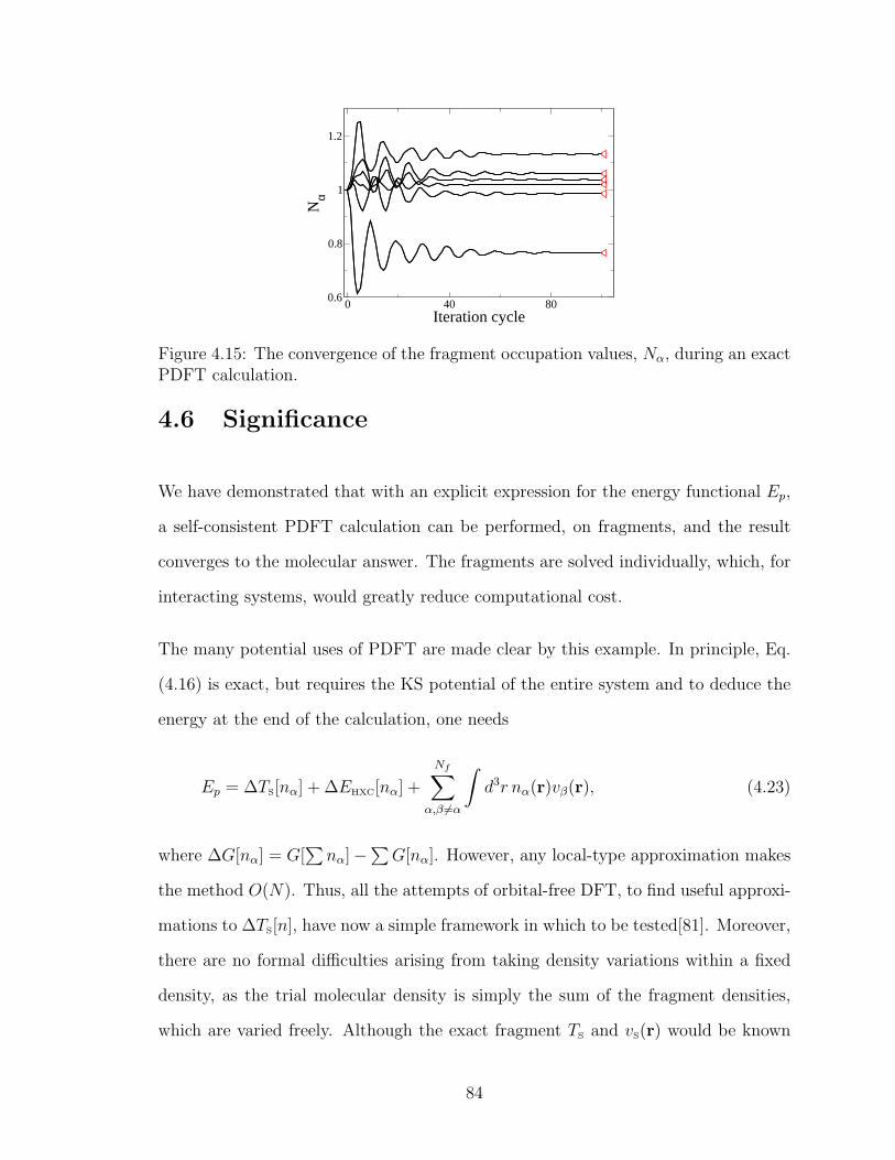
0 40 80Iteration cycle
0.6
0.8
1
1.2
Nα
Figure 4.15: The convergence of the fragment occupation values, Nα, during an exactPDFT calculation.
4.6 Significance
We have demonstrated that with an explicit expression for the energy functional Ep,
a self-consistent PDFT calculation can be performed, on fragments, and the result
converges to the molecular answer. The fragments are solved individually, which, for
interacting systems, would greatly reduce computational cost.
The many potential uses of PDFT are made clear by this example. In principle, Eq.
(4.16) is exact, but requires the KS potential of the entire system and to deduce the
energy at the end of the calculation, one needs
Ep = ∆TS[nα] + ∆EHXC[nα] +
Nf∑
α,β 6=α
∫
d3r nα(r)vβ(r), (4.23)
where ∆G[nα] = G[∑
nα]−∑
G[nα]. However, any local-type approximation makes
the method O(N). Thus, all the attempts of orbital-free DFT, to find useful approxi-
mations to ∆TS[n], have now a simple framework in which to be tested[81]. Moreover,
there are no formal difficulties arising from taking density variations within a fixed
density, as the trial molecular density is simply the sum of the fragment densities,
which are varied freely. Although the exact fragment TS and vS(r) would be known
84

during a calculation, approximations for ∆TS would take full advantage of any can-
cellation of errors. For embedding calculations, a simple approximation would be to
treat the system plus some fraction of its environment (a border region) exactly, and
all the rest approximately. Since the KS potential is typically near-sighted, such a
scheme should converge rapidly.
For the dissociation of molecules, one can also see how to ensure correct dissociation
energies within PDFT: simply constrain occupations to be those of the isolated frag-
ments. For H2, we constrain the spin occupations on the fragments to be (0,1) and
vice versa. Of course, this is what happens when symmetry is broken as the bond
is stretched, and the difficulty is in producing a scheme that seamlessly goes over
to (1/2,1/2) occupations as R reduces to the equilibrium value. The value of our
formalism is that it produces a framework for both addressing these questions and
constructing approximate solutions.
There is a simple adiabatic connection formula for PDFT. Consider scaling all bond
lengths between fragments by λ−1 (again keeping intrafragment densities fixed), where
0 < λ ≤ 1. For each λ, we find those molecular densities whose fragment densities
match those of our molecule, and define the corresponding partition energy, Ep(λ).
At λ = 1, we have the original molecule; as λ → 0, the bonds become large and
the fragments do not interact, so that Ep(0) = 0. For intermediate λ, the molecular
density is simply that of the fragments, overlapped a distance R/λ apart. Then
E = Ef +
∫ 1
0
dλdEp(λ)
dλ. (4.24)
This allows all the methods of traditional intermolecular symmetry-adapted pertur-
bation theory (SAPT)[82] to be applied to this problem, but with the advantage
that the fragment densities remain fixed. Interestingly, because the fragments will
85

generally have dipole moments, the partition energy decays as 1/R3, so that the in-
tegrand above behaves as λ2. (For physical systems that are well-separated and have
attractive van der Waals forces, such effects must be cancelled by analogous terms in
Erel).
There has been considerable previous work on schemes designed to allow a frag-
ment calculation of a larger molecule, either within the framework of orbital-free
DFT or atomic deformation potentials, sometimes producing the same (or similar)
equations. Among the earliest, Cortona’s crystal potential (later called embedding
potential)[83, 90] is an intuitive prescription for vp(r). But our formalism reproduces
the exact solution of the original problem, using only quantities that are already de-
fined in KS-DFT. For example, this is not possible in general without the ensemble
definition of Eq. (4.5), which produces the correct self-consistent occupations (unlike,
e.g., the self-consistent atomic deformation method[84, 85], where this choice leads to
a basis set dependence[86]) . We also never freeze the total density[87, 88, 89], but
only ever consider it as a sum of fragment densities. This avoids ever needing density
variations that are limited by some frozen total density, which produces bizarre func-
tional derivatives, different from those of KS DFT. None of these issues arise once
smooth (e.g. local or gradient-corrected) approximations are made to the kinetic en-
ergy functional[83, 90, 85], but they are vital in a formally exact theory. Thus the
present PDFT can be regarded as a formal exactification (and therefore justification)
of these pioneering works.
86

Chapter 5
Conclusion
In this work I have discussed two new approaches to the electronic structure problem.
Both these approaches share the same goal of making electronic structure calculations
faster and more accurate.
The first is potential functional theory which used semiclassical methods to find direct
expressions for the density and kinetic energy density as functionals of the potential.
These expressions were derived for an arbitrary potential in a box with hard walls and
with no turning points at the Fermi energy, which although quite primitive already
provides us with much insight. Extending this approach to the more general case that
involves turning points is part of ongoing work, as is the possibility of extending it to
three dimensional systems. If this were to be done, it could be used to massively speed
up DFT using the scheme investigated in Ref. [91]. In any case, the main motivation
behind the area of potential functional theory is to understand and improve DFT.
This work allows us to explain why local approximations like Thomas-Fermi or LDA
exchange work so well, namely they are the dominate terms in the semiclassical limit.
We can also see why gradient corrections like GEA fail to the improve upon local
87

approximations as they miss the important quantum oscillation corrections. It also
explains why generalized gradient approximations had to be developed before DFT
became accurate enough for chemistry, and allowed us to provide an ex post facto
derivations of the previously empirical B88 GGA exchange functional. It may also be
possible to fix the GEA by including these quantum corrections.
The second approach is partition density functional theory whereby the electronic
structure of a system can be found by performing calculations on smaller fragments
making up the system. Due to the scaling of computational time with system size for
current electronic structure methods, working on smaller pieces would greatly speed
up such calculations. Unfortunately this speed up comes at the price of having to
approximate more unknown pieces as a density functionals, however there is good
reason to believe that the quantities involved may be quite amenable to approxima-
tion. PDFT may also help solve the problem DFT suffers from when dissociating
atoms as the unknown partition energy Ep[n] must vanish in this limit, making it
easier to approximate.
It is interesting to speculate how the two approaches may influence eachother. In
PDFT, the most difficult term to approximate is ∆TS[n], the difference between the
molecular kinetic energy and the fragment kinetic energies as a density functional.
From test calculations and experience, I expect that local or semi-local approxima-
tions will not be enough to capture this difference, and it is mainly this difference that
causes the dip in the partition potential in a bonding region. However the kinetic
energy in an evanescent region between two atoms is exactly the kind of quantity
PFT allows us to find. Another interesting feature of PDFT is that different methods
could be used on the different fragments, so PDFT gives the exact prescription on
how to perform a QM/MM-like calculation. If in the eventually the density as a
potential functional is not accurate enough for chemical purposes, then it still may be
88

a cheap way to include quantum effects in a border region or solvation, PDFT would
be the correct tool to make use of this.
89

Bibliography
[1] Inhomogeneous electron gas, P. Hohenberg and W. Kohn, Phys. Rev. 136, B 864
(1964).
[2] Self-consistent equations including exchange and correlation effects, W. Kohn and
L.J. Sham, Phys. Rev. 140, A 1133 (1965).
[3] An Undulatory Theory of the Mechanics of Atoms and Molecules, E. Schrodinger,
Phys. Rev. 28, 1049 (1926).
[4] Semiclassical approximations in wave mechanics, M. V. Berry and K. E. Mount,
Rep. Prog. Phys. bf 35, 315 (1972).
[5] A Primer in Density Functional Theory, ed. C. Fiolhais, F. Nogueira, and M.
Marques (Springer-Verlag, NY, 2003).
[6] see dft.uci.edu
[7] Excited states from time-dependent density functional theory, P. Elliott, F. Furche,
and K. Burke, in Reviews in Computational Chemistry, eds. K. B. Lipkowitz and
T. R. Cundari, (Wiley, Hoboken, NJ, 2009), pp 91-165.
[8] Generalized gradient approximation made simple, J.P. Perdew, K. Burke, and
M. Ernzerhof, Phys. Rev. Lett. 77, 3865 (1996); 78, 1396 (1997) (E).
90

[9] Density-functional exchange-energy approximation with correct asymptotic behav-
ior, A. D. Becke, Phys. Rev. A 38, 3098 (1988).
[10] Development of the Colle-Salvetti correlation-energy formula into a functional
of the electron density, C. Lee, W. Yang, and R. G. Parr, Phys. Rev. B 37, 785
(1988).
[11] Density-functional thermochemistry. III. The role of exact exchange, A.D. Becke,
J. Chem. Phys. 98, 5648 (1993).
[12] Jacobs Ladder of Density Functional Approximations for the Exchange-
Correlation Energy, J. P. Perdew and K. Schmidt, in Density Functional Theory
and Its Applications to Materials, eds. V. E. Van Doren, K. Van Alsenoy, and P.
Geerlings (American Institute of Physics, Melville, NY, 2001).
[13] Kohn-Sham exchange potential exact to first order in ρ(K → 0)/ρ0, P.R. An-
toniewicz and L. Kleinman, Phys. Rev. B 31, 6779 (1985).
[14] Correlation energy of an electron gas with a slowly varying high density, S.-K.
Ma and K. A. Brueckner, Phys. Rev. 165, 18 (1968).
[15] Density functional calculations of molecular bond energies, A. D. Becke, J. Chem.
Phys. 84, 4524 (1986).
[16] Static dielectric response of the electron gas, C. Bowen, G. Sugiyama, and B. J.
Alder, Phys. Rev. B 50, 14838 (1994).
[17] Static Response and Local Field Factor of the Electron Gas, S. Moroni, D. M.
Ceperley, and G. Senatore, Phys. Rev. Lett. 75, 689 (1995).
[18] Improved lower bound on the indirect Coulomb energy, E. H. Lieb and S. Oxford,
Int. J. Quantum Chem. 19, 427 (1981).
91

[19] The calculation of atomic fields, L.H. Thomas, Proc. Camb. Phil. Soc. 23, 542
(1926).
[20] A statistical method for the determination of some atomic properties and the
application of this method to the theory of the periodic system of elements E.
Fermi, Zeit. Fur Physik 48, 73 (1928).
[21] The Thomas-Fermi approximation in quantum mechanics N. H. March, Adv. in
Phys. 6, 1 (1957).
[22] Thomas-Fermi model: The leading correction, J. Schwinger, Phys. Rev. A 22,
1827 (1980); Thomas-Fermi model: The second correction, ibid. 24, 2353 (1981).
[23] Quantum corrections to the Thomas-Fermi equation, D.A. Kirzhnits, Sov. Phys.
JETP 5, 64 (1957).
[24] Generalized gradient approximation for solids and their surfaces, J. Perdew, A.
Ruzsinszky, G.I. Csonka, O.A. Vydrov, G.E. Scuseria, L.A. Constantin, X. Zhou,
and K. Burke, arXiv:0707:2088
[25] Potential Functionals: Dual to Density Functionals and Solution to the v-
Representability Problem, W. Yang, P.W. Ayers, and Q. Wu, Phys. Rev. Lett.
92, 146404 (2004)
[26] Thomas-fermi and related theories of atoms and molecules, E.H. Lieb, Rev. Mod.
Phys. 53, 603 (1981).
[27] Hellmann-Feynman, virial, and scaling requisites for the exact universal density
functionals. Shape of the correlation potential and diamagnetic susceptibility for
atoms, M. Levy and J.P. Perdew, Phys. Rev. A 32, 2010 (1985).
[28] A new chemical concept: Shape chemical potentials, G.K.L. Chan and N.C.
Handy, J. Chem. Phys. 109, 6287 (1998).
92

[29] Relevance of the slowly-varying electron gas to atoms, molecules, and solids, J.
P. Perdew, L. A. Constantin, E. Sagvolden, and K. Burke, Phys. Rev. Lett. 97,
223002 (2006).
[30] Recursion representation of gradient expansion for free fermion ground state in
one dimension, L. Samaj and J.K Percus, J. Chem. Phys. 111, 1809 1999.
[31] Quantum density oscillations in an inhomogeneous electron gas, W. Kohn and
L. Sham, Phys. Rev. 137, A1697 (1965).
[32] Density-functional exchange-correlation through coordinate scaling in adiabatic
connection and correlation hole, M. Levy, Phys. Rev. A 43, 4637 (1991).
[33] Tight bound and convexity constraint on the exchange-correlation-energy func-
tional in the low-density limit, and other formal tests of generalized-gradient ap-
proximations, M. Levy and J.P. Perdew, Phys. Rev. B 48, 11638 (1993); ibid.,
55, 13321 (1997)(E).
[34] Nonuniform coordinate scaling requirements for exchange-correlation energy, M.
Levy and H. Ou-Yang, Phys. Rev. A 42, 651 (1990).
[35] Exchange-correlation energy of a metallic surface: Wave-vector analysis, D.C.
Langreth and J.P. Perdew, Phys. Rev. B 15, 2884 (1977).
[36] Theory of nonuniform electronic systems. I. Analysis of the gradient approxima-
tion and a generalization that works, D.C. Langreth and J.P. Perdew, Phys. Rev.
B 21, 5469 (1980).
[37] The surface energy of a bounded electron gas, J. Harris and R.O. Jones, J. Phys.
F 4, 1170 (1974).
93

[38] Exchange and correlation in atoms, molecules, and solids by the spin-density-
functional formalism, O. Gunnarsson and B.I. Lundqvist, Phys. Rev. B 13, 4274
(1976).
[39] Some remarks on scaling relations in density functional theory, W. Yang, in
Density Matrices and Density Functionals, eds. R. Erdahl and V. H. Smith, Jr.
(D. Reidel Publishing Company, Dordrecht, The Netherlands, 1987), pp 499-506.
[40] A new functional with homogeneous coordinate scaling in density functional the-
ory: F[ρ,λ], M. Levy, W. Yang, and R. G. Parr, J. Chem. Phys. 83, 2334 (1985).
[41] Rationale for mixing exact exchange with density functional approximations, J.P.
Perdew, M. Ernzerhof, and K. Burke, J. Chem. Phys. 105, 9982 (1996).
[42] The adiabatic connection method: A non-empirical hybrid, K. Burke, M. Ernz-
erhof, and J.P. Perdew, Chem. Phys. Lett. 265, 115 (1997).
[43] Mixing exact exchange with GGA: When to say when, K. Burke, J.P. Perdew,
and M. Ernzerhof, in Electronic Density Functional Theory: Recent Progress and
New Directions, eds. J.F. Dobson, G. Vignale, and M.P. Das (Plenum, NY, 1998),
page 57.
[44] Construction of the adiabatic connection, M. Ernzerhof, Chem. Phys. Lett. 263,
499 (1996).
[45] Generalized gradient approximation for solids and their surfaces, J. Perdew, A.
Ruzsinszky, G.I. Csonka, O.A. Vydrov, G.E. Scuseria, L.A. Constantin, X. Zhou,
and K. Burke, Phys. Rev. Lett. 100, 136406 (2008).
[46] Adiabatic connection from accurate wavefunction calculations, D. Frydel, W. Ter-
illa, and K. Burke, J. Chem. Phys. 112, 5292 (2000).
94

[47] Comparison of approximate and exact density functionals: A quantum monte
carlo study, C.J. Umrigar and X. Gonze, in High Performance Computing and
its Application to the Physical Sciences, Proceedings of the Mardi Gras 1993
Conference, edited by D. A. Browne et al. (World Scientific, Singapore, 1993).
[48] Accurate exchange-correlation potentials and total-energy components for the he-
lium isoelectronic series, C.J. Umrigar and X. Gonze, Phys. Rev. A 50, 3827
(1994).
[49] Thomas-Fermi Theory Revisited, E.H. Lieb and B. Simon, Phys. Rev. Lett. 31,
681 (1973).
[50] Semiclassical Origins of Density Functionals, P. Elliott, D. Lee, A. Cangi, and
K. Burke, Phys. Rev. Lett. 100, 256406 (2008).
[51] OPMKS: atomic DFT program, University of Frankfurt, Germany., E. Engel
[52] Local correlation energies of two-electron atoms and model systems, C.J. Huang
and C.J. Umrigar, Phys. Rev. A 56, 290 (1997).
[53] Exact Condition on the Kohn-Sham Kinetic Energy, and Modern Parametriza-
tion of the Thomas-Fermi Density, D. Lee, K. Burke, L.A. Constantin, J.P.
Perdew, submitted to J. Chem. Phys. (Fall 2008).
[54] Semiclassical theory of atoms, B.-G. Englert, Lect. Notes Phys. 300 (1988).
[55] Sixth-order term of the gradient expansion of the kinetic-energy density func-
tional, D. R. Murphy, Phys. Rev. A 24, 1682 (1981).
[56] Numerical test of the sixth-order gradient expansion for the kinetic energy: Ap-
plication to the monovacancy in jellium, Z. D. Yan, J. P. Perdew, T. Korhonen,
and P. Ziesche, Phys. Rev. A 55, 4601 (1997).
95

[57] Exchange and correlation energy in a nonuniform fermion fluid, M. Rasolt and
D. J. W. Geldart, Phys. Rev. B 34, 1325 (1986).
[58] Density-functional thermochemistry. III. The role of exact exchange, A. D. Becke,
J. Chem. Phys. 98, 5648 (1993).
[59] Thomas-Fermi model: The leading correction, J. Schwinger, Phys. Rev. A 22,
1827 (1980); Thomas-Fermi model: The second correction, ibid. 24, 2353 (1981).
[60] Semiclassical atom, B.-G. Englert and J. Schwinger, Phys. Rev. A 32, 26 (1985).
[61] C. Froese-Fischer, The Hartree-Fock method for atoms: a numerical approach
(Wiley, New York, 1977).
[62] Condition on the Kohn-Sham Kinetic Energy, and Modern Parametrization of
the Thomas-Fermi Density, D. Lee, L. A. Constantin, J. P. Perdew, and K. Burke,
J. Chem. Phys. 130, 034107 (2009).
[63] Unified theory of exchange and correlation beyond the local density approxima-
tion, J. P. Perdew, in Electronic Structure of Solids 91, eds. P. Ziesche and H.
Eschrig (Akademie Verlag, Berlin, 1991), pp. 11.
[64] Derivation of a generalized gradient approximation: The PW91 density func-
tional, K. Burke, J. P. Perdew, and Y. Wang, in Electronic Density Functional
Theory: Recent Progress and New Directions, eds. J. F. Dobson, G. Vignale, and
M. P. Das (Plenum, NY, 1998), pp. 81.
[65] R. M. Dreizler and E. K. U. Gross, Density Functional Theory (Springer-Verlag,
Berlin, 1990).
[66] The wave mechanics of an atom with a non-coulomb central field I. Theory and
methods, D. R. Hartree, Proc. Cambridge Phil. Soc. 24, 89 (1928).
96

[67] Naherungsmethode zur Losung des quantenmechanischen Mehrkorperprobleme,
V. Fock, Z. Phys. 61, 126 (1930).
[68] Peter Fulde, Electron Correlations in Molecules and Solids (Springer-Verlag,
Berlin, 1991).
[69] On the foundations of Chemical Reactivity Theory, M. H. Cohen and A. Wasser-
man, J. Phys. Chem. A 111, 2229 (2007).
[70] On hardness and electronegativity equalization in Chemical Reactivity Theory,
M. H. Cohen and A. Wasserman, J. Stat. Phys. 125, 1125 (2006).
[71] Density-functional theory for fractional particle number: Derivative discontinu-
ities of the energy, J. P. Perdew, R.G. Parr, M. Levy, and J.L. Balduz, Jr., Phys.
Rev. Lett. 49, 1691 (1982).
[72] What do the Kohn-Sham orbitals mean? How do atoms dissociate?, J.P. Perdew,
in Density Functional Methods in Physics, edited by R.M. Dreizler and J. da
Providencia (Plenum, NY, 1985), p. 265.
[73] Charge Transfer in Partition Theory, M. H. Cohen, A. Wasserman, R. Car, and
K. Burke, J. Phys. Chem. A 113, 2183 (2009).
[74] Kohn-Sham method as a free-energy minimization at infinite temperature, R.G.
Parr and Y.A. Wang, Phys. Rev. A 55, 3226 (1997).
[75] From electron densities to Kohn-Sham kinetic energies, orbital energies,
exchange-correlation potentials, and exchange-correlation energies, Q. Zhao, R.C.
Morrison, and R.G. Parr, Phys. Rev. A 50, 2138 (1994).
[76] On the Optimal Mixing of the Exchange Energy and the Electron-Electron Inter-
action Part of the Exchange-Correlation Energy, O. Gritsenko, R. van Leeuwen,
and E.J. Baerends, Int. J. Quantum Chem. 30, 1375 (1996).
97

[77] A direct optimization method for calculating density functionals and exchange-
correlation potentials from electron densities, Q. Wu and W. Yang, J. Chem. Phys.
118, 2498 (2003).
[78] Correlation energies for some two- and four-elactron systems along the adiabatic
connection in density functional theory, F. Colonna, A. Savin, J. Chem. Phys.
110, 2828 (1999).
[79] Separation of the exchange-correlation potential into exchange plus correlation:
An optimized effective potential approach, C. Filippi, C.J. Umrigar, and X. Gonze,
Phys. Rev. A 54, 4810 (1996).
[80] Algorithm to derive exact exchange-correlation potentials from correlated densi-
ties in atoms, K. Peirs, D. Van Neck, and M. Waroquier, Phys. Rev. A 67, 012505
(2003).
[81] The energy-differences based exact criterion for testing approximations to the
functional for the kinetic energy of non-interacting electrons, Y. A. Bernard, M.
Dulak, J. W. Kaminski, T. A. Wesolowski, J. Phys. A: Math. Theor. 41, 055302
(2008).
[82] Dispersion Energy from Density-Functional Theory Description of Monomers, A.
J. Misquitta, B. Jeziorski, and K. Szalewicz, Phys. Rev. Lett. 91, 033201 (2003).
[83] Self-consistently determined properties of solids without band-structure calcula-
tions P. Cortona, Phys. Rev. B 44, 8454 (1991).
[84] Self-consistent deformation method for application of density functional theory L.
L. Boyer, H.T. Stokes, M.M. Ossowski, and M.J. Mehl, Phys. Rev. B 78, 045121
(2008).
98

[85] Development of a Kohn-Sham like potential in the self-consistent atomic defor-
mation model M.J. Mehl, H.T. Stokes, and L.L. Boyer, J. Phys. Chem. Solids 57,
1405 (1996).
[86] Water molecule by the self-consistent atomic deformation method, M. M. Os-
sowski, L. L. Boyer, M. J. Mehl, and M. R. Pederson, Phys. Rev. B 68, 245107
(2003).
[87] Frozen density functional approach for ab inition calculations of solvated
molecules T.A. Wesolowski and A. Warshel, J. Phys. Chem. A 97, 8050 (1993).
[88] Electronic-structure calculations by first-principles density-based embedding of ex-
plicitly correlated systems N. Govind, Y.A. Wang, and E.A. Carter, J. Chem. Phys.
110, 7677 (1999).
[89] Self-consistent embedding theory for locally correlated configuration interaction
wave functions in condensed matter P. Huang, and E.C. Carter, J. Chem. Phys.
125, 084102 (2006).
[90] Direct determination of self-consistent total energies and charge densities of
solids: A study of the cohesive properties of the alkali halides P. Cortona, Phys.
Rev. B 46, 2008 (1992).
[91] Adiabatic Connection and the KohnSham Variety of PotentialFunctional Theory,
E. K. U. Gross and C. R. Proetto, J. Chem. Theory Comput. 5, 844 (2009).
99

Appendices
A Exchange energy for non-interacting Beryllium
The limit of the inequality, Eq. (3.56), is the Hartree-exchange functional evaluated on
the density of the corresponding non-interacting system. Since the g.s. orbitals which
sum to this density are known analytically (they are simply hydrogenic orbitals), we
may calculate the exact Hartree-exchange value.
Written in spherical coordinates, r = |r|, the 1s and 2s hydrogenic orbitals are:
φ1s(r) =
(
Z3
π
)1/2
e−Zr , (A.1)
φ2s(r) =
(
Z3
32π
)1/2
(2 − Zr)e−Zr/2 . (A.2)
For beryllium, both these orbitals are doubly occupied, giving the total density as
n(r) = 2|φ1s(r)|2 + 2|φ2s(r)|
2 . (A.3)
The Hartree energy is defined by Eq. (2.42), however in the special case of spherical
100

densities it may be written as:
U [n] =1
2
∫ ∞
0
dr (f [n](r))2 , (A.4)
where
f [n](r) = 4π
∫ ∞
r
dr′ r′n(r′) , (A.5)
and we use square brackets to indicate that it is a functional of the density. The
exchange energy for a spin-unpolarized system is:
EX = −21
2
occ∑
i,j
∫
d3r
∫
d3r′φ∗
i (r)φ∗j(r
′)φj(r)φi(r′)
|r − r′|, (A.6)
where the factor 2 is due to spin, and the sum is over occupied orbitals only, in this
case 1s and 2s. If we define a new quantity, n(r):
n(r) = φ1s(r)φ2s(r) , (A.7)
then we may write
EX = −2 (U [n1s] + 2U [n] + U [n2s]) . (A.8)
We can use Eq. (A.5) and Eq. (A.4) for each term separately and then combine to
find the total exchange energy. The answer will be equivalent to solving Eq. (A.6)
using the orbitals, however this method avoids performing integrals involving 1/|r−r′|
and, in this case, are easy to solve using integration by parts. The values for Hartree,
exchange and their sum are:
U [n] =5 × 23 × 431
2634=
49565
5184= 9.561 ,
101

EX = −59 × 71 × 73
2736= −
305797
93312= −3.277 ,
EHX =383 × 1531
2736=
586373
93312= 6.284 .
B Finding EF
Solving the quantization condition for the Fermi energy:
θF(L) =
∫ L
0
dx kF(x) = (N + 0.5)π (B.9)
can be done via a Newton-like method. An initial guess for ǫF is made, usually the
flat box value:
ǫgF
=
[
(N + 1/2)π
L
]2
This will differ from the correct ǫF by ∆ǫ, which we will assume to be small. Then
we can expand Eq. (B.9) as
θ1(L, ǫgF) +
∆ǫ
2τ1(L, ǫ
gF) = (N + 1/2)π (B.10)
thus ∆ǫ may be calculated. This can be added to the first initial guess ǫgF to find a
new initial guess and the process repeated until ǫF is found to the accuracy required.
102

C Charge-neutral scaling inequality
We follow the steps in deriving Eq. (3.48) but applied to the charge neutral scaling
defined in Eq. (3.42). Taking nζ1/ζ(r) as a trial density for the v(r) system, then the
variational principle states:
F [nζ1/ζ ] + V [nζ
1/ζ ] ≥ F [n] + V [n] , (C.11)
where nζ(r) is the exact density for the scaled potential vζ(r). Conversely, use nζ(r)
as a trial density for the vζ(r) system:
F [nζ ] + ζ7/3V [n] ≥ F [nζ ] + ζ7/3V [nζ1/ζ ] (C.12)
where we have used V ζ [nζ ] = ζ7/3V [n]. Combining these inequalities gives:
F [nζ ] − F [nζ ]
ζ7/3≥ F [n] − F [nζ
1/ζ ] , (C.13)
which may be written as
∆F ζ [nζ1/ζ ] ≥ ∆F ζ [n] , (C.14)
with
∆F ζ [n] = F [n] −F [nζ ]
ζ7/3. (C.15)
103