UNIVERSITY OF CALIFORNIA, IRVINE · 2012 Ph.D., University of California, Irvine: Irvine, CA; Earth...

UNIVERSITY OF CALIFORNIA, IRVINE

Ecosystem Controls and the Impacts of Climate on Vegetation Production and Patterns in California’s Mountains

DISSERTATION

Submitted in partial satisfaction of the requirements for the degree of

DOCTOR OF PHILOSOPHY

in Earth System Science

by

Aaron W. Fellows

Dissertation Committee:

Professor Michael L. Goulden, Chair

Professor James T. Randerson

Professor Diane Pataki

2012

All rights reserved

INFORMATION TO ALL USERSThe quality of this reproduction is dependent on the quality of the copy submitted.

In the unlikely event that the author did not send a complete manuscriptand there are missing pages, these will be noted. Also, if material had to be removed,

a note will indicate the deletion.

All rights reserved. This edition of the work is protected againstunauthorized copying under Title 17, United States Code.

ProQuest LLC.789 East Eisenhower Parkway

P.O. Box 1346Ann Arbor, MI 48106 - 1346

UMI 3494315

Copyright 2012 by ProQuest LLC.

UMI Number: 3494315

ii

TABLE OF CONTENTS

LIST OF FIGURES ....................................................................................................................... iv

LIST OF TABLES ......................................................................................................................... vi

ACKNOWLEDGMENTS ............................................................................................................ vii

CURRICULUM VITAE .............................................................................................................. viii

ABSTRACT OF THE DISSERTATION ...................................................................................... ix

Chapter 1: Introduction ................................................................................................................... 1

1.1 Climate change impacts on vegetation .............................................................................. 1

1.2 Tree mortality .................................................................................................................... 2

1.3 The underlying causes of tree mortality ............................................................................ 3

1.4 The importance of tree mortality in ecosystems ................................................................ 4

1.5 Climate change and species distribution shifts .................................................................. 5

1.6 Climate controls on forest functions .................................................................................. 7

1.7 Approach ........................................................................................................................... 8

1.8 Dissertation Outline ........................................................................................................... 9

Chapter 2: Rapid vegetation redistribution in Southern California following the early 2000s drought .......................................................................................................................................... 11

2.1 Introduction ..................................................................................................................... 11

2.2 Methods ........................................................................................................................... 13

2.3 Results ............................................................................................................................. 18

2.4 Discussion ........................................................................................................................ 30

2.5 Conclusions ..................................................................................................................... 36

Chapter 3: How does a semiarid forest survive at the warm and dry edge of its range? ............. 37

3.1 Introduction ..................................................................................................................... 37

3.2 Methods ........................................................................................................................... 39

3.3 Results ............................................................................................................................. 46

3.4 Discussion ........................................................................................................................ 57

Chapter 4: Can the short-term meteorological controls on canopy photosynthesis explain the long-term relationship between climate and vegetation along an elevation gradient? ................. 66

4.1 Introduction ..................................................................................................................... 66

iii

4.2 Methods ........................................................................................................................... 68

4.3 Results ............................................................................................................................. 78

4.4 Discussion ........................................................................................................................ 87

Chapter 5: Has Fire Suppression Increased the Amount of Carbon Stored in Western US Forests?....................................................................................................................................................... 93

5.1 Abstract ............................................................................................................................ 93

5.2 Introduction ..................................................................................................................... 94

5.3 Methods ........................................................................................................................... 95

5.4 Results ............................................................................................................................. 97

5.5 Discussion ...................................................................................................................... 100

Chapter 6: Conclusion................................................................................................................. 104

6.1 Overview ....................................................................................................................... 104

6.2 General Conclusions ...................................................................................................... 106

6.3 Things to have done differently ..................................................................................... 108

6.4 Future Work ................................................................................................................... 109

References ................................................................................................................................... 110

iv

LIST OF FIGURES

Figure 1.1: Photograph of dead conifer trees………………………………………………….…..2 Figure 1.2: Factors leading to widespread tree dieback…………………………...……..………..3

Figure 1.3: Example of Species Distribution Shift………………………………………………..6 Figure 1.4: Short- and Long-term controls on GPP………..……………………………..……….8 Figure 2.1: Map of elevation gradient……………………………………………………………13

Figure 2.2: Species fraction cover with elevation………………………………………………..20

Figure 2.3: Live and dead conifer fraction cover .…………………………………….…………21

Figure 2.4: Composite midmontane species distribution……………………………..………….23

Figure 2.5: Composite subalpine species distribution……………………………….…………..24

Figure 2.6: Conifer diameter size distribution…………………………………………….……..26

Figure 2.7: Reported bark beetle outbreaks……………………………………………….….….28

Figure 2.8: Reported bark beetle outbreaks with temperature record…………………….….….29

Figure 3.1: Map of the study area……………………………………………………………….40

Figure 3.2: Environmental data time series at site……………………………………….……...47

Figure 3.3: Soil matric water potential…………………………………………………………..48

Figure 3.4: Predawn and midday water potential time series…………………………...……….49

Figure 3.5: Leaf level Amax time series…..…………………………………………..……….….50

Figure 3.6: Amax, leaf area, and GEE time series…..…………………………………….……....52

Figure 3.7: GEE time series for 2007, 2008, and 2009…..………………………………………53

Figure 3.8: GEE response to temperature….………………………………………….…………54

Figure 3.9: GEE response to vapor pressure deficit………………………………….………….55

Figure 3.10: 2009 water balance………………………………………………………...……….56

v

Figure 3.11: Low temperature carbon sink to source transition…….…………………………...61

Figure 4.1: Runoff vs. P- PM ET……………………….……………………………………….73

Figure 4.2: GPPshort calculation………………………………………………………………….75

Figure 4.3: EVI-GPP regression………………………………………………………...………76

Figure 4.4: Radiosonde and tower temperature time series……………………………...………79

Figure 4.5: Transect meteorological gradient………………………………………….………...80

Figure 4.6: Transect vegetation gradient………………………………………………………...81

Figure 4.7: Light response curve……………………………………………………...…………82

Figure 4.8: Temperature scalar…………………………………………………………………..83

Figure 4.9: Precipitation and GPP time series…………………………………………….……..84

Figure 4.10: Fraction of unstressed observation with elevation……………………..…..………86

Figure 4.11: GPPlong and GPPshort with elevation………………………………………………...87

Figure 5.1: Tree density and carbon storage by tree size……………………………….…..….100

vi

LIST OF TABLES

Table 2.1: Terms and calculations........................................................................…………...…..16

Table 2.2: Species distribution properties……………………………………….………….……25

Table 2.3: Conifer seedlings…………………………………………………………….….……27

Table 3.1: Tree density, basal area, and plant functional type…..…………………………..…..46

Table 3.2: Conifer leaf gas exchange…..………………………………………………...………51 Table 3.3: Ecosystem level properties………………………………………………………...…53 Table 3.4: Climate constraints on tower productivity…..…………………………………….…55 Table 4.1: Site information……………………………………….…………………………...…77 Table 5.1: Stand density and carbon stored in aboveground live biomass for various categories…………………………………………………………..……………………….…....98

vii

ACKNOWLEDGMENTS

I thank Michael Goulden for the opportunities, his insight into how ecosystems work,

guidance, and continued support. He was integral to my learning process through his creative

ideas, his understanding of the scientific process, and his questions and constructive criticism.

This dissertation would not have been possible without his guidance.

I also thank my dissertation committee, Jim Randerson and Diane Pataki, for their review

of this manuscript and helpful comments and questions.

I owe a debt of gratitude to Greg Winston, Scot Parker, Anne Kelly, and Ray Anderson

who helped collect data that was important in this dissertation. Mike Lawler, Francesca

Hopkins, Adrian Rocha, Andrew Mcmillan, Liza Litvak, and Heather McCarthy also provided

key insights into challenges that I faced along the way and helped to broaden and deepen my

scientific interests.

The Department of Earth System Science was a great place to learn about a breadth of

ideas. I am grateful to the entire faculty and my fellow students, who helped to change the way I

view the Earth. I would also like to extend thanks to the administrative staff, who provided

logistical support, with a special thanks to Cynthia Dennis and Morgan Sibley.

I am also thankful to Susan Hicks and my family for their support and encouragement.

The American Geophysical Union provided permission to include copyrighted material.

Grants awarded to Michael Goulden from the Kearney Foundation and the DOE Program

for Ecosystem Research provided funding for this research.

viii

CURRICULUM VITAE

Aaron W. Fellows EDUCATION: 2012 Ph.D., University of California, Irvine: Irvine, CA; Earth Systems Science

Thesis title: “Ecosystem Controls and the Impacts of Climate on Vegetation Production and Patterns in California’s Mountains.”

2008 M.S., University of California, Irvine: Irvine, CA; Earth System Science 2004 B.S., University of Pittsburgh, Pittsburgh, PA; Physics & Astronomy 2004 B.A., University of Pittsburgh, Pittsburgh, PA; Architectural Studies WORK EXPERIENCE: 2011 Instructor, University of California, Irvine; Irvine, CA, ESS 1 2005-present Graduate Student Researcher, University of California, Irvine; Irvine, CA 2006- 09 Teaching Assistant, University of California, Irvine, Earth System Science, Geology, Field Methods, and Land Interactions 2004 (summer) Field Assistant, University of Pittsburgh, P.I.: Dr. Walter Carson PUBLICATIONS: Refereed Journal Articles Fellows, A. W., and M. L. Goulden (2008), Has fire suppression increased the amount of carbon stored in western U.S. forests?, Geophys. Res. Lett., 35, L12404,doi:10.1029/2008GL033965. Non-refereed Conference Presentations 2010 Fellows, Aaron and Michael Goulden. "Climate contributes to zonal forest mortality in Southern California’s San Jacinto Mountains." Poster presentation at American Geophysical Union, Annual Meetings, Dec. 2010. 2007 Fellows, Aaron and Michael Goulden. “Does Western US forest thickening increase carbon stored in aboveground biomass?” Poster presentation at American Geophysical Union, Annual Meetings, Dec. 2007.

ix

ABSTRACT OF THE DISSERTATION

Ecosystem Controls and the Impacts of Climate on Vegetation Production and Patterns in California’s Mountains

By

Aaron W. Fellows

Doctor of Philosophy in Earth System Science

University of California, Irvine, 2012

Professor Michael L. Goulden, Chair

Climate change is anticipated to have widespread impacts on the biosphere, including

redistribution of vegetation and increases in tree mortality. In California, climate change is

predicted to lead to warmer and possibly drier conditions. The response of vegetation to these

changes remains uncertain due to our limited understanding of the sensitivity of vegetation to

weather and the range of potential responses. This dissertation addresses these uncertainties by

examining the effects of climate-mediated tree mortality and weather controls on vegetation in

California’s mountains.

Climate-mediated tree mortality occurred in 2002-04 in the semi-arid San Jacinto

Mountains, CA. Conifer tree mortality was widespread, rapid, and focused at low elevations.

This pattern of tree mortality was consistent with reduced precipitation associated with climate

variability. Increased mortality at low elevation rapidly drove mid-montane vegetation

distributions upslope.

x

Low elevation forests are thought to be vulnerable to climate change, but a limited

understanding of their function constrains predictions of possible responses to changes in

climate. We found that low elevation mixed conifer forests in Southern California maintain a

year-round growing season by continuing carbon uptake in the cool winters, and extracting water

stored from deep soils in the dry summers. Low elevation forests may be sensitive to certain

changes in climate including increased atmospheric vapor pressure deficit and reductions in

precipitation.

We hypothesized that reduced temperatures at high elevations and increased temperatures

and reduced water availability at low elevations shape elevation patterns of canopy level

photosynthesis in the San Jacinto Mountains. Short-term meteorological controls on canopy

photosynthesis were insufficient to predict the elevational pattern of production. Additional

controls may also be important, including controls on leaf-area, feedbacks and thresholds to

growth, fire disturbances, and edaphic properties.

Ecosystem level processes may also be affected by fire suppression. Increased forest

stem density due to fire suppression in Western US forests is thought to account for a portion of

the North American carbon sink. Stem density increased in California’s mountains from 1930s-

1990s, but this did not appear to increase carbon stored in aboveground biomass due to a

concomitant loss of large trees.

1

Chapter 1: Introduction

1.1 Climate change impacts on vegetation

There is growing concern that global climate change will have large impacts on the

biosphere and that climate change has already led to shifts in the phenology, species

distributions, community composition, and changes in the structure and function of ecosystems

(for reviews: [McCarty, 2001; Parmesan, 2006; Parmesan and Yohe, 2003; Walther et al.,

2002]). Recent attention has focused on the likelihood that tree mortality will increase with

climate change, and that recent tree mortality may reflect ongoing climate change [Adams et al.,

2009; van Mantgem et al., 2009].

In California, climate change is expected to lead to warmer and perhaps drier conditions,

with a possible reduction in precipitation and a likely temperature increase of 1.5°-4.5°C by 2100

[Cayan et al., 2008; Seager and Vecchi, 2010; Seager et al., 2007]. Recent widespread tree

mortality [Walker, 2006] and species distribution shifts (eg. [Kelly and Goulden, 2008]) that

coincided with climate trends indicate that montane vegetation in California can respond rapidly

to shifts in climate. However, the extent, magnitude, and sensitivity to climate change remains

uncertain.

2

1.2 Tree mortality

Increased accounts of tree mortality are being reported globally [Allen et al., 2010].

Western North America has undergone widespread conifer mortality, including in British

Columbia, Idaho, the Southwest US, and Southern California [Allen et al., 2010; Breshears et

al., 2005; Raffa et al., 2008; Walker, 2006].

Drought driven tree mortality occurred in California in the early 1990s [Savage, 1994]

and again in the early 2000s [Walker, 2006]. Conifer tree mortality in the early 2000s was very

high with an average of 20-100 mature stems dying per hectare (Fig.1; [Minnich, 2007; Walker,

2006]). In response to high tree mortality and forest fires in the early 2000s, Minnich [2007]

commented: “this episode may quite possibly become one of the great transformations in

California vegetation since the beginning of European settlement.”

Figure 1: Photograph of dead conifer trees. Standing dead conifer trees in the San Jacinto Mountains bear witness to widespread conifer tree mortality that occurred between 2002-04.

3

1.3 The underlying causes of tree mortality

The proximate cause of recent widespread tree mortality in the Western US was bark

beetle outbreak [Raffa et al., 2008]. The underlying causes may be more complex. Predisposing

factors, such as overstocking, air pollution, or climate change may leave forests weakened and

susceptible to widespread tree mortality (Fig. 2; [Mueller-Dombois, 1988] ). Periodic

perturbations in climate, such as a severe drought, may act as precipitating factors that weaken

the forests further. Weakened forests are susceptible to stand-level dieback by biotic agents,

which is often the modifying factor. Savage [1994] suggested that stand thickening due to fire

suppression, along with chronic air pollution, predisposed Southern California’s forests to high

mortality and that a drought around 1990 triggered bark beetle outbreaks that led to widespread

tree mortality in the region [Savage, 1994].

Figure 2: Factors leading to widespread tree dieback (cf. [Mueller-Dombois, 1988] ).

The complexity and interaction of these factors underscore the difficulty of tree mortality

attribution. Nonetheless, recent studies point to climate as a key factor driving increased tree

mortality [Adams et al., 2009; Allen et al., 2010]. Breshears et al. [2005] found that Southwest

4

US pinyon pine mortality at a focus site reached 90% in response to drought and above average

temperatures. Kurz et al. [2008] estimated that tree mortality from bark beetle outbreaks

converted portions of British Columbia forests from a small net carbon sink to a large net carbon

source, and linked this event with weather. Background mortality in the Western US has also

increased, coincident with recent warming trends [van Mantgem et al., 2009].

The growing reports of tree mortality, the well-established link with drought, and

possible links with increased temperature, indicate that climate is important [Allen et al., 2010].

Recent studies have also pointed out mechanisms that link tree mortality with a drier and warmer

climate, such as increased cavitation, increased carbon starvation, or possible changes in

carbohydrate allocation, which in turn weaken trees to bark beetle outbreak [Adams et al., 2009;

Sala, 2009; Sperry and Tyree, 1990].

1.4 The importance of tree mortality in ecosystems

Tree mortality plays an important role in ecosystems by altering population and

community structure, shifting live biomass to necromass, and changing light, nutrient, and

moisture availabilities [Franklin et al., 1987]. The death of a tree removes it from a population,

while creating new resources and habitats. Widespread tree mortality may also have appreciable

impacts on carbon, energy and water cycles [Adams et al., 2010].

Widespread mortality in Southern California’s mountains had an immediate and direct

human impact. Remaining snags threatened people and property with falling debris. Dead trees

increased fuel loads leaving forests and mountain towns vulnerable to catastrophic fire [Walker,

2006]. In response to the increased tree mortality of the early 2000s and increased fuel loads, the

US Forest Service thinned small vegetation and removed dead trees in portions of the San

5

Jacinto Mountains [USDA, 2007]. This forest management was intended to both improve forest

health and reduce the risk of fires in the Mount San Jacinto State Park and the mountain towns of

Idyllwild and Pine Cove, CA. Thinning and removal of dead vegetation was extensive in the

lower mixed conifer ecotone and required numerous work hours, improvement of small roads,

and the removal of trees from steep mountain slopes using heavy machinery and helicopters.

Tree mortality focused at the margin of a species’ range may also drive a rapid vegetation

redistribution. Understanding the patterns of climate/weather mediated tree mortality, such as

the tree mortality that occurred in the early 2000s in Southern California, is important for

understanding: 1) the sensitivity of montane vegetation to certain climate drivers and 2) how

vegetation may redistribute under climate change.

1.5 Climate change and species distribution shifts

Montane climate gradients are typically characterized by a decrease in temperature and

an increase in precipitation with elevation. Vegetation rises and falls in abundance with changes

in climate along these montane gradients [Stephenson, 1990; Urban et al., 2000; Whittaker and

Niering, 1975]. Climate change is anticipated to shift both montane climate gradients and

vegetation distributions upslope [Hayhoe et al., 2004]. A climate envelope approach assumes

that as the climate warms and dries with climate change, cooler and wetter montane climates will

shift upslope and vegetation will follow; individuals near the dry or warm parts of their species’

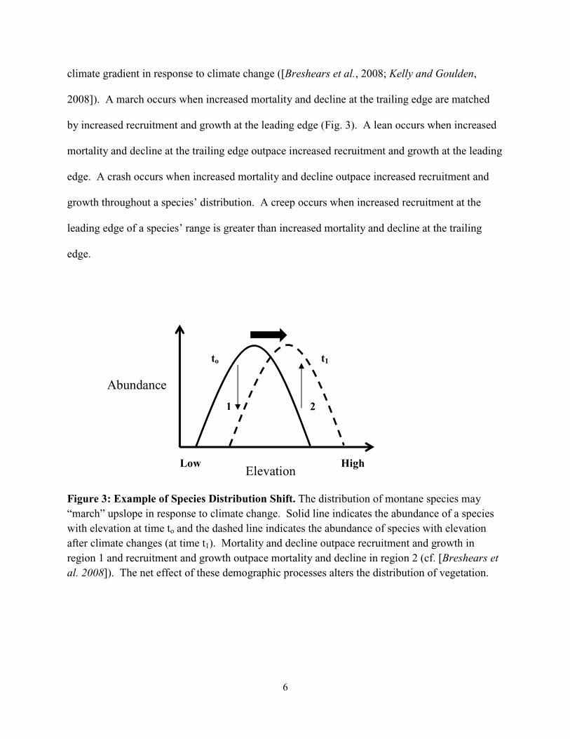
range will decline or die and new regions will open upslope to recruitment and growth (Fig. 3).

The type of redistribution, however, depends on how forest demography changes along the

climate gradient. Species’ distributions may “march,” “lean,” “crash,” or “creep” along a

6

climate gradient in response to climate change ([Breshears et al., 2008; Kelly and Goulden,

2008]). A march occurs when increased mortality and decline at the trailing edge are matched

by increased recruitment and growth at the leading edge (Fig. 3). A lean occurs when increased

mortality and decline at the trailing edge outpace increased recruitment and growth at the leading

edge. A crash occurs when increased mortality and decline outpace increased recruitment and

growth throughout a species’ distribution. A creep occurs when increased recruitment at the

leading edge of a species’ range is greater than increased mortality and decline at the trailing

edge.

Figure 3: Example of Species Distribution Shift. The distribution of montane species may “march” upslope in response to climate change. Solid line indicates the abundance of a species with elevation at time to and the dashed line indicates the abundance of species with elevation after climate changes (at time t1). Mortality and decline outpace recruitment and growth in region 1 and recruitment and growth outpace mortality and decline in region 2 (cf. [Breshears et al. 2008]). The net effect of these demographic processes alters the distribution of vegetation.

Abundance

Elevation High Low

1 2

to t1

7

1.6 Climate controls on forest functions

The response of ecosystems to climate change remains uncertain, in part, due to our

limited understanding of controls on ecosystem processes, such as carbon uptake. Gross Primary

Production (GPP) is the annual gross carbon uptake into an ecosystem; GPP provides a measure

of the carbon available for vegetation respiration, growth, and defense, and is important in tree

growth and survival. GPP is governed by a number of variables or controls, including light,

temperature, and water availability among others [Chapin et al., 2002]. Understanding the

physical controls on GPP is important for predicting how forests will respond to climate change.

Understanding forest function is particularly important at warm and dry range margins as these

are thought to be especially vulnerable to climate change (see Fig. 3).

We can think about the impacts of the physical environment on GPP in terms of short-

term and long-term controls. Short-term controls, such as light, temperature, and water

availability, caused by weather have a direct and immediate effect on plant and ecosystem gas

exchange. Long-term climate equilibrated controls affects carbon uptake at long time scales by

influencing leaf area, plant size, plant density, plant-species composition, and soil resources (Fig.

4). Determining the relative importance of short- and long-term controls is important for

understanding how vegetation may respond to climate.

8

Figure 4: Short- and long-term controls on GPP.

1.7 Approach

Southern California montane forests provide an especially useful system for investigating

the effects of climate and weather on vegetation because: 1) the local vegetation distributions are

thought to be strongly controlled by climate, 2) climate change is anticipated to have a regional

impact, and 3) recent changes, including tree mortality and species distribution shifts, have been

linked to weather and climate.

Understanding how climate and weather impact vegetation is complicated, in part, due to

the multiple temporal and spatial scales at which they affect ecosystem processes. This

dissertation used multiple approaches to gain perspective on these different temporal and spatial

scales. We made ecosystem level measurements at a single field site in a low elevation mixed

Meteorology; Light, Temp, & Plant Available Water

GPP

Climate

Soil properties

Plant Size, LAI, Species

Short-term Long-term

9

conifer forest to understand: 1) temporal variations in productivity from seconds to years, and 2)

the processes that occur as vegetation responds to weather. We addressed spatial patterns by

focusing on an elevation gradient to understand the potential impacts of climate changes on

vegetation [Crimmins et al., 2011; Kelly and Goulden, 2008; Lenoir et al., 2008]. Spatial

patterns of meteorology with elevation were determined using weather stations and radiosonde

temperature profiles. Vegetation cover was determined on the western slopes of the San Jacinto

Mountains using sampling transects, and productivity was determined using remote sensing

based Enhanced Vegetation Index [Huete et al., 2002].

1.8 Dissertation Outline

Chapter 2: We investigated widespread tree mortality that occurred in Southern California

forests between 2002-04 [Minnich, 2007; Walker, 2006]. We wanted to know: 1) how the early

2000s Southern California tree mortality varied with elevation, 2) whether the mortality

impacted species’ distributions and 3) whether the mortality was unique in a historical context.

This study addresses possible patterns of vegetation redistribution that may occur with changes

in weather and climate and the links between particular climate events and the redistribution of

vegetation that occurs as a result of associated tree mortality.

Chapter 3: In principle, forests located at their warm and dry climatic range limit would be at

greatest risk from climate change. We wanted to determine: 1) how temperature, atmospheric

drought stress, and soil water drought impact mixed conifer production and 2) the mechanisms

that allowed a mixed conifer forest to survive at its warm and dry range limit.

10

Chapter 4: Temperature and water availability place strong first order physiological controls on

GPP [Law et al., 2002]. In principle, reduced water availability is thought to limit GPP at low

elevations and cold temperatures are thought to limit GPP at high elevations in montane

California. We considered how temperature and water availability shape the pattern of GPP with

elevation. We wanted to know: 1) how GPP is governed by short-term controls of temperature

and water availability, 2) how temperature and water availability vary with elevation in the San

Jacinto Mountains, 3) how might the elevation pattern of GPP be shaped by the short-term

controls of temperature and water availability, and 4) does this short-term pattern agree with the

long-term climate equilibrated pattern of GPP with elevation.

Chapter 5: In addition to climate change, fire suppression in Western US forests is thought to

have large impacts on the structure and function of Western US ecosystems. Fire suppression

has led to an increase in stem density, which is thought to contribute to the North American

carbon sink. We considered the effects of fire suppression on carbon stored in aboveground live

biomass by accounting for changes in forest stem density and concomitant shifts in forest

structure.

Chapter 6: In the final chapter, I draw together the main conclusions of each chapter, address

potential shortcomings, and suggest future work.

11

Chapter 2: Rapid vegetation redistribution in

Southern California following the early 2000s drought

2.1 Introduction

California is expected to warm 1.5 to 4.5ºC by 2100 with global climate change [Cayan

et al., 2008], while precipitation is expected decline [Seager and Vecchi, 2010]. Climate

envelope models indicate that cooler and wetter climates will shift upslope and northward, and

vegetation will follow. Individual organisms near the dry or warm parts of their species’ range

will decline or die, while new regions open upslope to recruitment and growth. In particular, tree

mortality focused at the low elevation warm and dry edge of species’ ranges may drive species’

distributions upslope.

Widespread tree mortality associated with pest or pathogen outbreaks occurred in

Western North America over the last decade [Allen et al., 2010; Breshears et al., 2005; Raffa et

12

al., 2008; Walker, 2006]. In many cases, drought coupled with warm temperature was

considered an underlying factor. There is widespread suspicion that this mortality is similar to

what may occur under climate change [Allen et al., 2010].

Several studies have attributed recent changes in species distribution to changes in

climate. Comparisons with historical vegetation surveys have found an upslope shift in species’

distribution consistent with regional changes in temperature (eg. [Lenoir et al., 2008]). Kelly

and Goulden [2008] found that the cover-weighted mean elevation of 9 of the 10 most widely

spread species along a Southern California elevation transect shifted upslope by ~65 m, a result

that was consistent with regional climate trends. Ecotone shifts have been attributed to weather

and climate (eg. [Allen and Breshears, 1998; Beckage et al., 2008]), and local shifts in plant

distribution may occur rapidly in response to climate events. We are still uncertain, however,

about the possible patterns of vegetation redistribution that may occur with changes in weather

and climate and, in particular, the links between particular climate events and the redistribution

of vegetation that occurs as a result of associated tree mortality.

We investigated the widespread tree mortality that occurred in Southern California

montane forests between 2002-04, which followed a severe and prolonged drought [Walker,

2006]. We sought to understand the processes that lead to rapid redistribution of species cover.

We wanted to know if the early 2000s Southern California tree mortality 1) had an elevational

pattern, 2) impacted species’ distributions and 3) was unique in a historical context.

13

2.2 Methods

2.2.1 Site

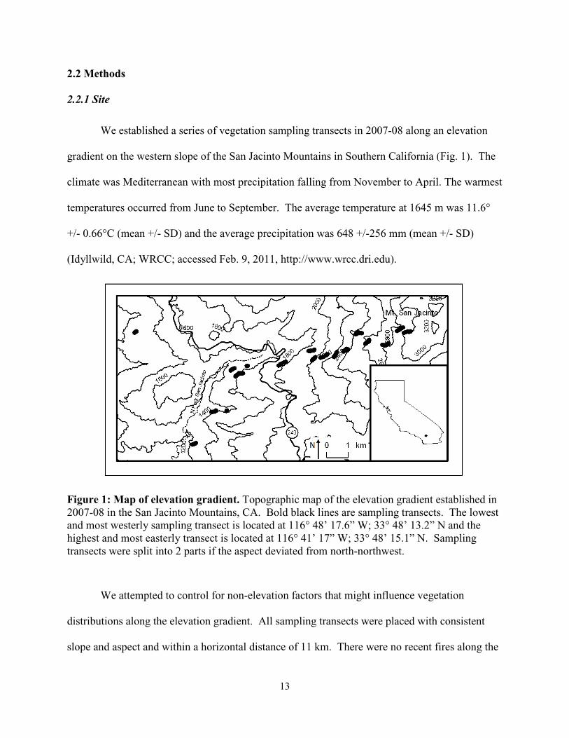
We established a series of vegetation sampling transects in 2007-08 along an elevation

gradient on the western slope of the San Jacinto Mountains in Southern California (Fig. 1). The

climate was Mediterranean with most precipitation falling from November to April. The warmest

temperatures occurred from June to September. The average temperature at 1645 m was 11.6°

+/- 0.66°C (mean +/- SD) and the average precipitation was 648 +/-256 mm (mean +/- SD)

(Idyllwild, CA; WRCC; accessed Feb. 9, 2011, http://www.wrcc.dri.edu).

Figure 1: Map of elevation gradient. Topographic map of the elevation gradient established in 2007-08 in the San Jacinto Mountains, CA. Bold black lines are sampling transects. The lowest and most westerly sampling transect is located at 116° 48’ 17.6” W; 33° 48’ 13.2” N and the highest and most easterly transect is located at 116° 41’ 17” W; 33° 48’ 15.1” N. Sampling transects were split into 2 parts if the aspect deviated from north-northwest.

We attempted to control for non-elevation factors that might influence vegetation

distributions along the elevation gradient. All sampling transects were placed with consistent

slope and aspect and within a horizontal distance of 11 km. There were no recent fires along the

14

elevation gradient, except for a small segment of the lowest sampling transect that last burned in

1974, and sampling transects below 1661 m, which last burned in 1924. Timber harvest and

grazing ended in the early 1900s. Soils were coarse grained and derived from granodiorite

across the entire elevation gradient (Soil Map from http://websoilsurvey.nrcs.usda.gov/).

2.2.2 Field observations of species distributions and mortality

Cover

We measured conifer tree cover in 2007-08 on 300-m one-dimensional sampling

transects that followed elevation isocontours. The sampling transects were located at 122 m

elevation intervals from 1295 m to 3002 m (Fig. 1). We determined cover by measuring the

length of each tree canopy projected onto the one-dimensional sampling transect. Sampling

transects were positioned along consistent slopes with north-northwest aspect to reduce the

confounding effects of topography. Sampling transects were broken into segments if the aspect

deviated from north-northwest. We recorded live and dead cover by species along each transect.

Dead trees had died within five years; they had lost most to all of their needles, retained branches

to ~0.25 in diameter, had some bark sloughing off, and were in a similar state of decay. Almost

all of the dead trees in this state of decay remained standing at the time of the survey.

Calculations and assumptions

The fraction cover of a species was calculated as the sum of species’ cover divided by the

length of the sampling transect (for species j: Fraction Coverj=∑ cover of species j on sampling

transect (m) / 300 m). Live07-08 was calculated as the fraction cover of live vegetation measured

15

in 2007-08 (for species j: Live07-08,j=∑ live coverj on sampling transect in meters/ 300 m; Table

1). Dead07-08 was the fraction cover of dead vegetation measured in 2007-08 (for species j:

Dead07-08,j=∑ dead coverj on sampling transect in meters/ 300 m). Live02 was the sum of live and

dead fraction cover measured in 2007-08 (for species j: Live02,j=∑ Live07-08,j + Dead07-08,j).

Mortality was calculated as the sum of a species dead fraction cover divided by the sum of live

and dead fraction cover (for species j: Mortalityj = ∑ Dead07-08,j / ∑ Live02,j).

Our approach assumed that live cover prior to the widespread tree mortality in 2002 was

equal to the sum of live and dead cover measured in 2007-08. However, dead tree crowns may

have contracted from their original shape by the time we measured cover, which would have us

underestimate Dead07-08. Moreover, growth and infilling of living trees may have increased

Live07-08. Our measurements, therefore, provide a conservative estimate of mortality and would

tend to minimize any trend in mortality with elevation.

We determined fraction cover and mortality for two broad conifer tree groups:

midmontane and subalpine. The midmontane conifer group included Abies concolor, Pinus

lambertiana, P. coulteri, P. jeffreyi, P. ponderosa, and Calocedrus decurrens species. The

subalpine conifer group included Pinus contorta and P. flexilis species.

We also analyzed conifer tree distributions and mortality at the species level. The cover-

weighted mean elevation for each species was calculated by summing the product of species’

cover and elevation over all elevations for a species and dividing by the sum of that species

cover over all elevations (for species j: cover-weighted mean elevationj = ∑ (fraction coverj on

sampling transect * elevation of that sampling transect) / ∑ fraction coverj over all sampling

transects); Table 1).

16

Term Definition Calculation

Live07-08 Sum of species’ 2007-08 live cover divided by sampling transect length

Σ measured live cover (m)/300 m

Dead07-08 Sum of species’ 2007-08 dead cover divided by sampling transect length

Σ measured dead cover (m)/300 m

Live02 Estimated fraction of live cover on transect in 2002

Live07-08 + Dead07-08

Cover-weighted mean elevation

Center of a species’ distribution Σ (Fraction cover*elevation) at each elevation / Σ Fraction cover over all elevations; Fraction cover could be Live07-08, Live02, or Dead07-08

Mortality Proportion of dead cover Dead07-08/ Live02

Normalized cover

Species’ fraction cover normalized by the largest fraction cover of that species on any one transect along the entire elevation gradient

Σ (Fraction cover for spj/ Maximum Fraction cover for spj on gradient)

Table 1: Terms and calculations.

We pooled Pinus coulteri, P. jeffreyi, and P. ponderosa into a yellow pine group, and P.

contorta and P. flexilis into a subalpine group. In both cases, we were unable to unambiguously

identify all dead pines to species. The effect of tree mortality on species’ cover-weighted mean

elevation was determined by subtracting the estimated 2002 cover-weighted mean elevation from

the 2007-08 cover-weighted mean elevation. We tested if this difference was significantly

different from zero using a two tailed t-test.

We normalized the fraction cover of each species on each transect by the maximum

fraction cover of that species found on any sampling transect on the entire elevation gradient (for

species j: normalized coverj = fraction coverj on sampling transect / fraction covermax,j; where

fraction covermax,j = maximum fraction cover of species j found on the entire elevation gradient;

17

Table 1). We constructed normalized distributions averaged across species by setting the transect

nearest the cover-weighted mean elevation of each species to zero and averaging the normalized

covers corresponding to 122 m above and 122 m below the cover-weighted mean elevation.

Size Distribution

Diameter at breast height (DBH) of all conifer trees greater than or equal to 138 cm tall

was recorded in ten (100 m2) subplots equally spaced along each sampling transect. Conifer

seedlings (less than 138 cm tall) were counted in subplots above 1661 m elevation.

We calculated mean conifer tree density (stems ha-1) above and below 2200 m to

compare conifer size structure in high and low elevation forests. Live and dead conifer trees

were binned into 10 cm DBH size classes to estimate the forest structure before tree mortality.

2.2.3 Historical weather

We obtained historical records of annual precipitation, monthly mean temperature, and

annual temperature for the southern interior region from the California climate tracker website

([Abatzoglou et al., 2009]; downloaded Jan. 19, 2011; http://www.wrcc.dri.edu/monitor/cal-

mon/frames_version.html). The southern interior region encompasses Southern California’s

Mountains. The climate tracker record combines multiple weather stations into a homogenous

record of precipitation and temperature from 1895 to 2009. Inspection of weather stations

included in the southern interior record showed that only 1 of the 17 stations reported data during

1895. Six stations reported data by 1905 and fourteen stations reported data by 1949. We used

the entire southern interior precipitation record to examine relative precipitation amounts over

18

the past ~100 years, and data from 1949 onwards to examine quantitative trends in precipitation

and temperature.

2.2.4 Historic tree mortality

We searched for historic reports of widespread tree mortality in The Los Angeles Times

newspaper using the Proquest database (accessed Feb 9, 2011, http://www.proquest.com/en-

US/). We searched the following terms: “beetle” and “san jacinto”; “beetle” and “san

bernardino”; “beetle” and “angeles national forest”; “beetle” and “san bernardino national

forest”; “beetle” and “idyllwild”, and “pine beetle”. We immediately rejected articles with titles

not referring to bark beetles or tree mortality, and reviewed the remaining articles. Articles that

reported widespread tree mortality or bark beetle outbreaks in Southern California were recorded

to the year and verified with governmental and scientific reports when possible.

2.3 Results

2.3.1 Species and Plant functional type distribution

The various conifer species covered discrete elevation ranges from 1417 m to the highest

transect at 3002 m (Fig. 2). Several species had large overlapping ranges. Midmontane conifers

species spanned 1417 m to 2758 m and subalpine conifer species spanned 2637 m to 3002 m

(Fig. 3). Total conifer cover peaked at 2271 m, which was near the midpoint of the conifer

range. Evergreen and deciduous oaks, including Quercus chrysolepis, Q. kelloggii, and Q.

wislizeni, contributed to non-conifer cover below 2149 m. Chaparral species, mostly

19

Arctostaphylos spp. and Adenostoma fasciculatum, contributed to non-conifer cover below

1539 m.

2.3.2 Recent weather and climate trends

Temperature increased in the southern interior region over the past ~60 years. Regional

temperatures have increased 0.0208 °C yr-1 since 1949 (p <0.01; linear regression, slope different

from 0). We determined the changes in the 11-year running standard deviation and an 11-year

running coefficient of variation of precipitation from 1949 to 2005. Precipitation variability

increased from 1949 to the 1980s and then declined. Precipitation amount has not changed

since 1949 (p=0.53; linear regression, slope different from 0).

Decreased precipitation and above average annual temperatures preceded the 2002-04

conifer mortality. Annual southern interior precipitation in 2002 was 48% of average and the 8th

lowest in the 116 year record. The five year preceding mean precipitation was 84% of average in

2002 and 69% of average in 2003. Annual southern interior temperature in 2002 was 0.82 °C

above average and the 11th warmest in the record.

20

Figure 2: Species fraction cover with elevation. Live07-08 at each sampling transect on the elevation gradient. Species include: Abies concolor (black circle), Calocedrus decurrens (open square), Pinus lambertiana (open triangle), and a yellow pine group, which included Pinus coulteri, P. ponderosa, and P. jeffreyi (black diamond). Subalpine species include: Pinus contorta (inverted open triangle) and P. flexilis (black square).

1200 1400 1600 1800 2000 2200 2400 2600 2800 30000

0.1

0.2

0.3

0.4

0.5

0.6

Fra

ctio

n C

over

Elevation (m)

Abies concolorCalocedrus decurrensPinus lambertianaP. coulteri, ponderosa, jeffreyi

P. contortaP. flexilis

Midmontane:

Subalpine:

21

Figure 3: Live and dead conifer fraction cover. a) Live07-08 and Dead07-08 midmontane and subalpine fraction cover. Midmontane species include: Abies concolor, Calocedrus decurrens, Pinus lambertiana, P. coulteri, P. ponderosa, and P. jeffreyi. Subalpine species include: Pinus contorta and P. flexilis. b) Conifer mortality (D; open triangle) including all conifers over the elevation gradient. Elevation (m) is in meters.

1200 1400 1600 1800 2000 2200 2400 2600 2800 30000

0.1

0.2

0.3

0.4

0.5

0.6

Con

ifer

Mor

talit

y

Elevation (m)

0

0.2

0.4

0.6

0.8

Fra

ctio

n C

over

Live07-08

Midmontane

Live07-08

Subalpine

Dead07-08

Midmontane

Dead07-08

Subalpine

r2 = 0.50, p < 0.01

a)

b)D(m) = -0.0003*m + 0.74

22

2.3.3 Mortality Patterns

Conifer mortality was 15% over the entire survey. The fraction of dead cover was

greatest from 1783 m to 2271 m reaching 9 to 18% (Fig 3). Conifer mortality increased with

decreasing elevation (Fig. 3; p<0.01; linear regression; slope different from zero). Nearly 40%

of the live 2002 conifer cover died at the lower conifer ecotone (Fig. 3).

We separated the conifers into midmontane and subalpine conifer groups. Midmontane

conifer mortality exceeded subalpine mortality (Fig. 3). Overall, midmontane conifer mortality

was 17%, whereas subalpine mortality was 3%. Midmontane conifer mortality increased with

decreasing elevation (Fig. 4, p=0.02; linear regression; slope different from zero). Subalpine

conifer tree mortality did not show a statistically significant trend with elevation (Fig. 5, p=0.32;

linear regression; slope different from zero).

We compared species’ mortality within the midmontane conifer group. Abies concolor,

Calocedrus deccurrens, Pinus lambertiana and Yellow Pine (Pinus coulteri, ponderosa, jeffreyi)

mortality was high, ranging from 9% to 25% over the elevation gradient (Table 2). The cover-

weighted mean elevation of dead cover was below the cover-weighted mean elevation of Live02

cover for each midmontane species (Table 2), indicating that midmontane conifer tree mortality

was focused in the lower portion of the species’ ranges. This mortality caused a 37 +/- 33 m

(mean +/- 95% CI; p=0.04) upslope shift in the midmontane conifer cover-weighted mean

elevation.

23

Figure 4: Composite midmontane species distribution. a) Live02 (black triangle) and Live07-08

(open triangle) midmontane composite species distributions. The composite species distributions were determined by setting the sampling transect nearest the Live02 cover-weighted mean elevation to zero for each midmontane species and then averaging the normalized cover of each species at the corresponding sampling transect above and below the cover-weighted mean elevation. Positive values are meters above and negative values are meters below the cover-weighted mean elevation. The center elevation is the cover-weighted mean elevation for each species. b) Conifer mortality (D; open triangle) over the composite species distribution. Elevation (m) is in meters.

0

0.2

0.4

0.6

0.8N

orm

aliz

ed C

over

Live02

Live07-08

-800 -600 -400 -200 0 200 400 600 8000

0.2

0.4

0.6

0.8

1

Con

ifer M

orta

lity

Elevation - Center Elevation (m)

r2 = 0.53, p = 0.02

b)

a)

D(m) = -0.0003*m + 0.13

24

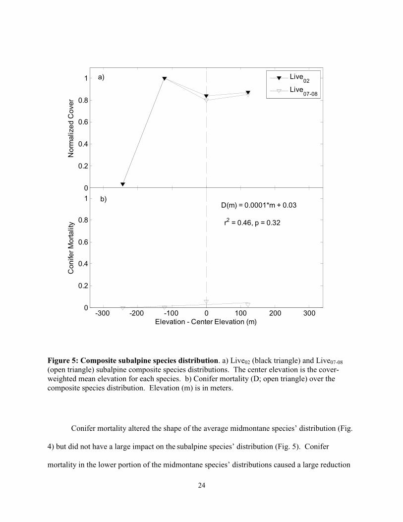
Figure 5: Composite subalpine species distribution. a) Live02 (black triangle) and Live07-08

(open triangle) subalpine composite species distributions. The center elevation is the cover-weighted mean elevation for each species. b) Conifer mortality (D; open triangle) over the composite species distribution. Elevation (m) is in meters.

Conifer mortality altered the shape of the average midmontane species’ distribution (Fig.

4) but did not have a large impact on the subalpine species’ distribution (Fig. 5). Conifer

mortality in the lower portion of the midmontane species’ distributions caused a large reduction

0

0.2

0.4

0.6

0.8

1N

orm

aliz

ed C

over

Live02

Live07-08

-300 -200 -100 0 100 200 3000

0.2

0.4

0.6

0.8

1

Con

ifer M

orta

lity

Elevation - Center Elevation (m)

r2 = 0.46, p = 0.32

a)

b)D(m) = 0.0001*m + 0.03

25

in live conifer cover at low elevations (Fig. 4). The pattern of subalpine conifer mortality

paralleled the Live02 subalpine species’ cover, resulting in a small -1 m change in the cover-

weighted mean elevation of these species.

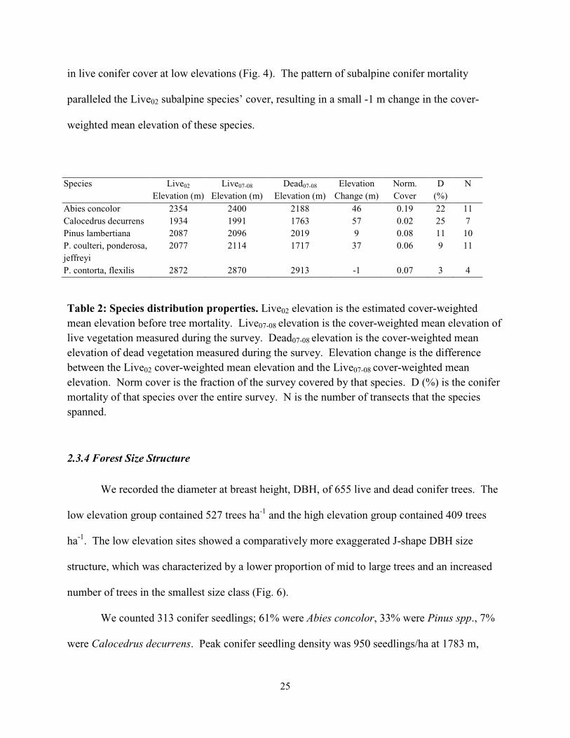
Species Live02

Elevation (m) Live07-08

Elevation (m) Dead07-08

Elevation (m) Elevation

Change (m) Norm. Cover

D (%)

N

Abies concolor 2354 2400 2188 46 0.19 22 11 Calocedrus decurrens 1934 1991 1763 57 0.02 25 7 Pinus lambertiana 2087 2096 2019 9 0.08 11 10 P. coulteri, ponderosa, jeffreyi

2077 2114 1717 37 0.06 9 11

P. contorta, flexilis 2872 2870 2913 -1 0.07 3 4

Table 2: Species distribution properties. Live02 elevation is the estimated cover-weighted mean elevation before tree mortality. Live07-08 elevation is the cover-weighted mean elevation of live vegetation measured during the survey. Dead07-08 elevation is the cover-weighted mean elevation of dead vegetation measured during the survey. Elevation change is the difference between the Live02 cover-weighted mean elevation and the Live07-08 cover-weighted mean elevation. Norm cover is the fraction of the survey covered by that species. D (%) is the conifer mortality of that species over the entire survey. N is the number of transects that the species spanned.

2.3.4 Forest Size Structure

We recorded the diameter at breast height, DBH, of 655 live and dead conifer trees. The

low elevation group contained 527 trees ha-1 and the high elevation group contained 409 trees

ha-1. The low elevation sites showed a comparatively more exaggerated J-shape DBH size

structure, which was characterized by a lower proportion of mid to large trees and an increased

number of trees in the smallest size class (Fig. 6).

We counted 313 conifer seedlings; 61% were Abies concolor, 33% were Pinus spp., 7%

were Calocedrus decurrens. Peak conifer seedling density was 950 seedlings/ha at 1783 m,

26

which was in the lower midmontane conifer forest (Table 3). We did not find a statistically

significant trend in conifer seedling densities with elevation. We did not find any seedlings

above the local adult tree species’ range.

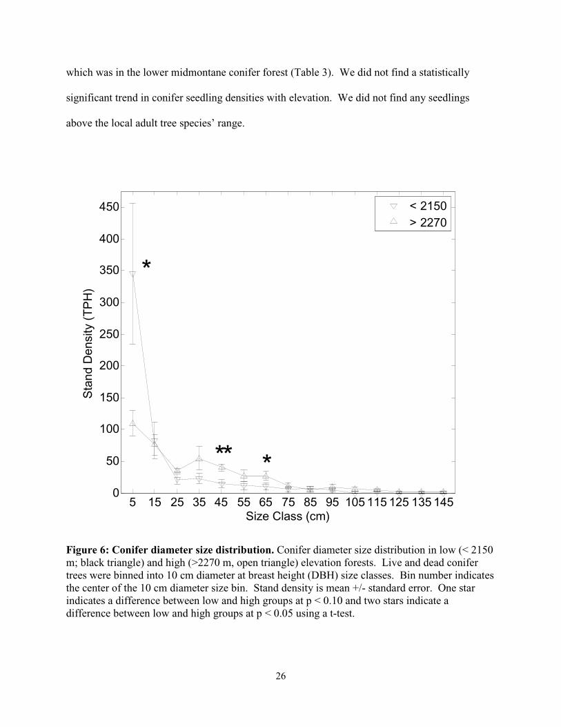
Figure 6: Conifer diameter size distribution. Conifer diameter size distribution in low (< 2150 m; black triangle) and high (>2270 m, open triangle) elevation forests. Live and dead conifer trees were binned into 10 cm diameter at breast height (DBH) size classes. Bin number indicates the center of the 10 cm diameter size bin. Stand density is mean +/- standard error. One star indicates a difference between low and high groups at p < 0.10 and two stars indicate a difference between low and high groups at p < 0.05 using a t-test.

5 15 25 35 45 55 65 75 85 95 105 115 125 135 1450

50

100

150

200

250

300

350

400

450

Size Class (cm)

Sta

nd D

ensi

ty (

TP

H)

< 2150> 2270

*

*

**

27

Elevation (m) Mid-montane seedlings (seedlings ha-1)

Subalpine seedlings (seedlings ha-1)

1661 170 0 1783 950 0 1905 670 0 2027 160 0 2149 260 0 2271 50 0 2393 40 0 2515 50 0 2637 150 10 2758 260 40 2880 0 30 3002 0 290 Table 3: Conifer seedlings. Midmontane and subalpine conifer seedling density (conifer trees with a height less than 138 cm).

2.3.5 Historical Context

The Los Angeles Times contained reports beginning in 1903 of episodic tree mortality

caused by bark beetle outbreaks. Bark beetles outbreaks were reported approximately every 15

years, with a large number of articles published between 1950 and 1960. There were often

several articles published in one year, or several consecutive years, likely indicating an extensive

bark beetle outbreak. Reported bark beetle outbreaks in Southern California were episodic and

coincided with periods of low precipitation (Fig. 7). Years with reported bark beetle outbreaks

had significantly lower annual precipitation and lower mean precipitation in the preceding five

years than years with no reports (p < 0.05). Reported bark beetle outbreaks in Southern

California also coincided with warmer annual temperature, though the correlation was weaker

(Fig. 8; p < 0.05). We found no correlation between winters temperatures and reported bark

beetle outbreaks (Fig. 8).

28

1900 1920 1940 1960 1980 2000 2020 100

200

300

400

500

600

700

800

900

1000

P (

mm

)

Time (year)

Figure 7: Reported bark beetle outbreaks with precipitation record. Bark beetle outbreaks reported in the Los Angeles Times newspaper (black circles) are plotted on top of the previous 5 year moving average (bold black line) of the annual southern interior precipitation record (light gray line).

29

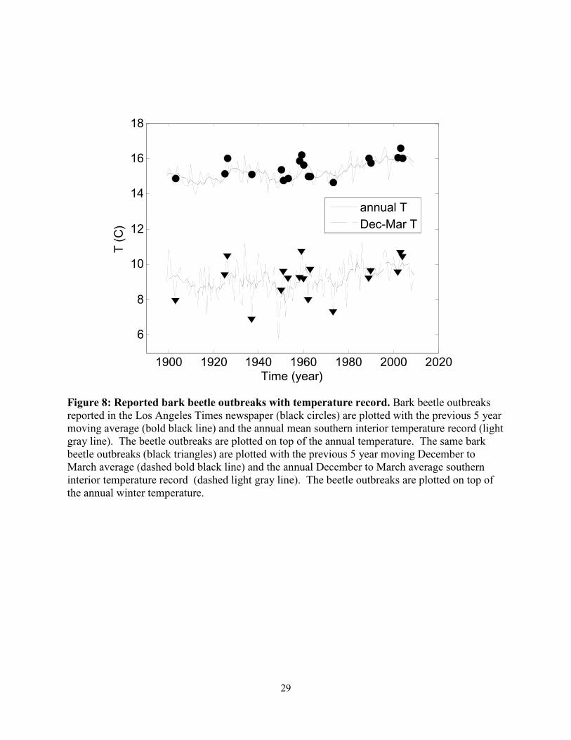
Figure 8: Reported bark beetle outbreaks with temperature record. Bark beetle outbreaks reported in the Los Angeles Times newspaper (black circles) are plotted with the previous 5 year moving average (bold black line) and the annual mean southern interior temperature record (light gray line). The beetle outbreaks are plotted on top of the annual temperature. The same bark beetle outbreaks (black triangles) are plotted with the previous 5 year moving December to March average (dashed bold black line) and the annual December to March average southern interior temperature record (dashed light gray line). The beetle outbreaks are plotted on top of the annual winter temperature.

1900 1920 1940 1960 1980 2000 2020

6

8

10

12

14

16

18T

(C

)

Time (year)

annual TDec-Mar T

30

2.4 Discussion

2.4.1 How do the patterns of species distribution and mortality compare with previous reports?

Conifer species covered discrete elevation distributions that were similar to the ranges

previously reported for California ([Whittaker and Niering, 1975], Fig. 2). Likewise, the rates of

conifer tree mortality observed were similar to those reported previously for Southern California

[Walker, 2006]. We found 15% conifer tree mortality over the entire gradient, which is in

agreement with the 12.7% of conifers >= 12.7 cm in diameter reported by Walker et al. [2006] to

have died between 2002-2004. We found high mortality in Calocedrus deccurrens (25%), Abies

concolor (23%), Pinus lambertiana (11%), and Yellow Pine (Pinus coulteri, ponderosa, jeffreyi)

(7%), which broadly agrees with the pattern reported by Walker et al. (2006), though they found

higher mortality in Pinus lambertiana (21%) and Yellow Pine (Pinus coulteri, ponderosa,

jeffreyi) (17%) and lower mortality in Abies concolor (17%) and far lower mortality in

Calocedrus deccurrens (0.2%). These differences may be attributed to the scope, objectives, and

methods of the two studies. Walker et al. [2006] reported tree mortality over a broader region

that included multiple mountain ranges and did not focus on elevation gradients.

The 15% conifer mortality we calculated for 2002-04 was far above the long-term

mortality. Ansley and Battles [1998] found baseline tree mortality in a Sierra Nevada old growth

forest was 0.6% yr-1. Stephenson and van Mantgem [2005] reported that average turnover, tree

mortality and recruitment, were less than 2% yr-1 in the Sierra Nevada Mountains. Minnich

[2007] speculated that the regional tree mortality between 2002-04 surpassed the combined

regional tree mortality over the last century.

31

2.4.2 What are the patterns of vegetation redistribution?

Midmontane conifer trees in the San Jacinto Mountains died at lower elevations (Fig. 3).

The rapid reduction in live midmontane conifer cover at low-elevation altered the distribution of

conifer cover and caused the midmontane distribution to skew upslope by 2007-08 (Fig. 4). The

rapid shift in midmontane species distribution led to a mean ~ 37 m upslope shift in the cover-

weighted mean elevation averaged across all midmontane conifers (Table 2).

Most species did not show a change in range extent. Abies concolor was the exception

with 100% mortality at its lowest elevation. In general, high conifer mortality near the lower

conifer ecotone broadened the range periphery, rather than shifted the lower ecotone boundary

[Jump et al., 2009]. We found no evidence of seedling recruitment to higher elevations,

indicating that the upper range extent was also static.

Patterns of vegetation redistribution in response to changes in climate include a “march,”

“lean,” “crash,” and “creep” [Breshears et al., 2008; Kelly and Goulden, 2008]. The pattern of

redistribution is a balance of forest demographic processes. A march is characterized by a shift in

the range margins and central tendency of a species along a climate gradient and is a result of

increased mortality and decline at the tailing edge matched by increased recruitment and growth

at the leading edge. A lean is characterized by a shift in the central tendency along the climate

gradient while range limits do not change and is a result of recruitment and growth at the leading

edge outpaced by mortality and decline at the trailing edge. A crash occurs when there is an

overall decline across a species’ range and is a result of mortality and decline outpacing

recruitment and growth throughout a species’ entire distribution. A creep occurs when a species’

distribution expands upslope and is a result of recruitment at the leading edge of a species’ range

32

outpacing mortality and decline at the trailing edge. Our observations were most consistent with

an increased lean in the early 2000s.

2.4.3 What are the likely causes of redistribution?

The 2002-04 mortality followed a period of decreased precipitation and above average

annual temperatures. In 2002, annual southern interior precipitation was 48% of average, which

was the 8th lowest in the 116 year record, and annual southern interior temperature was 102% of

average, which was the 11th warmest year on record. The five year preceding mean precipitation

was 84% of average in 2002 and 69% of average in 2003. This drought likely triggered the 2002-

04 bark beetle outbreak that led to widespread conifer tree death in Southern California [Walker,

2006].

Montane conifer forests in Southern California tend to be comparatively more water

limited at lower elevation than at higher elevation [see Chapter 4]. In these forests, precipitation

increases with elevation to ~1500 m, where it remains constant with elevation and Penman-

Monteith evapotranspiration increases with decreasing elevation, likely leading to reduced plant

available water at low elevations [see Chapter 4]. The early 2000s drought likely led to even

greater reductions in plant water availability in low and mid elevation forests.

Water stressed trees may be more susceptible to bark beetle attacks and mortality due to

reductions in carbohydrate allocation to defensive compounds [Adams et al., 2009; Sala, 2009].

Further, warmer temperatures may increase vulnerability to bark beetle outbreak by exacerbating

drought stress or by increasing tree pest metabolism directly, which can allow beetles overcome

tree defenses [Raffa et al., 2008]. The reduced water availability and higher temperatures

33

associated with the preceding drought likely increased the vulnerability of low elevation conifer

trees to the 2002-4 bark beetle attacks.

Predisposing factors may have additionally weakened these forests leaving them

vulnerable to drought driven beetle attack [Mueller-Dombois, 1988]. For example, high rates of

forest mortality in the San Jacinto Mountains during the early 1990s were attributed to air

pollution, stem densification, and drought [Savage, 1994].

Regional changes in climate may have also predisposed low elevation conifers to greater

mortality. The 0.0208 C yr-1 of regional warming over the past 60 years (Fig. 8) resulted in a

~3.5 m yr-1 upslope shift in temperature with elevation assuming a –0.006 C/m lapse rate (=temp

increase/lapse rate). The difference between potential evapotranspiration and precipitation in the

San Jacinto Mountain has also increased by approximately 2.667 mm yr-1 [Crimmins et al.,

2011]. These changes in climate may have reduced conifer tree vigor at their dry and warm

range extent, predisposing conifer trees to drought and beetle attack.

2.4.4 How did redistribution and mortality compare between midmontane and subalpine

forests?

Midmontane conifer mortality was high and focused in the low portion of the species’

ranges, whereas subalpine conifer mortality was low and independent of elevation. The

observed conifer mortality patterns were consistent with the hypothesis that the early 2000s

drought drove reductions in plant available water, and that these reductions in plant available

water were greatest at low elevations. Midmontane conifer distributions ranged from 1417 m to

2758 m (Fig. 3) and spanned a range of decreasing water limitation from low to high elevation.

34

Subalpine conifer tree distributions ranged above 2637 m, an area where water limitation may be

uncommon (Fig. 3).

2.4.5 Is species redistribution a common occurrence?

Southern California bark beetle outbreaks and conifer mortality have repeatedly occurred

over the past 100 years and are strongly associated with prolonged extended drought (Fig 7).

Los Angeles Times articles expressed alarm at the extent of some of these past outbreaks. For

example, a 1903 article titled “Pine Forests Doomed by Dakota Beetle” speculated that “at the

present rate of death among the large pine trees, it will be only a matter of a few years before the

forest will be destroyed.”

Redistribution of conifer vegetation may have occurred with past mortality, if mortality

was located at species’ range margins. Two pieces of evidence suggest that past conifer

mortality may have been greatest in low elevation conifer forests. First, the size structure of live

and dead conifer trees in low elevation forests showed a strong J-shape characterized by a large

number of small conifer trees and few moderate to large conifer trees (Fig 6). Bark beetles may

prefer moderate to large trees and past bark beetle outbreaks may have contributed to the J-

shaped structure. Previous conifer mortality, such as that reported in the early 1990s, may have

also been greatest at low elevations and shifted vegetation upslope [Savage, 1994]. Second, an

article published on January 29, 1950 in the Los Angeles Times was titled “Pine Beetle

Infestation Fight Began” and reported from Idyllwild, CA that the “greatest damage from the

pine bark beetles has occurred in the regions bordering the chaparral belts,” providing anecdotal

evidence of high tree mortality at low elevations.

35

Episodic tree mortality and subsequent regrowth may shift midmontane conifer

distributions in a response to natural climate variability. Decadal climate variability in California

has been linked to large scale oscillations in the Earth system, such as the Pacific Decadal

Oscillation (PDO; [Biondi, 2001; McCabe et al., 2004]) and El Niño–Southern Oscillation

(ENSO; [Cayan et al., 1999]). We found that episodic tree mortality coincided with periods of

prolonged low precipitation and warmer annual temperatures over the past 100 years (Fig 7, Fig

8). Seedling recruitment is also episodic in Western conifer forests and depends on multiple

biotic and abiotic factors that include climate [North et al., 2005; van Mantgem et al., 2006].

The growth of trees at tree line in montane California respond to similar climate variability

[Millar, 2004]. Shifts in demography, growth, and decline coupled with past climate variability

may have led to changes in vegetation distributions over the history of this forest: vegetation

distributions retracted when mortality was high at the trailing edge and expanded when

recruitment was high at the leading edge. The patterns of conifer mortality we observed may be

part of a natural cycle of differential expansions and contractions in the lower and upper parts of

species’ ranges associated with climate variability.

Recent studies have related changes in vegetation distributions with climate trends,

including a rapid shift in a low elevation ecotone in response to drought [Allen and Breshears,

1998] or a downslope shift in vegetation presence in response to reduced water deficit [Crimmins

et al., 2011]. Kelly and Goulden [2008] showed that vegetation cover “leaned” upslope in

response to changes in local climate. Attribution of biotic responses to global climate change,

however, is difficult especially at small spatial scales, over short time periods, and for single

events [Parmesan et al., 2011]. We found evidence that tree mortality has reoccurred over the

past 100 years in Southern California forests, and past mortality was correlated with climate

36

variability. This historic baseline of vegetation mortality underscores the difficulty in attributing

vegetation responses to global climate change in montane California.

2.5 Conclusions

Climate change is anticipated to drive vegetation distribution shifts. Our current

understanding is: 1) Shifts in vegetation distributions are important because they can change

range extents, change the probability of a species presence, and impact species’ cover across the

landscape, 2) Vegetation distributions appear to respond rapidly to certain climate drivers, and 3)

Vegetation distributions shifts can occur in discrete events. These results indicate that vegetation

distributions may respond rapidly to climate change, but predicting how vegetation distributions

will change will ultimately require sorting out the climate controls and feedbacks on forest

demographics and accurate predictions of regional climate.

37

Chapter 3: How does a semiarid forest survive at the

warm and dry edge of its range?

3.1 Introduction

Widespread tree mortality occurred during the last decade across Western North America

including British Columbia, Idaho, Colorado, the Southwest US, and Southern California [Allen

et al., 2010; Breshears et al., 2005; Raffa et al., 2008; Walker, 2006]. Similarly, background

mortality rates have increased in the Western US coincident with recent changes in climate [van

Mantgem et al., 2009]. Drought coupled with warm temperature was thought to contribute to

this mortality [Adams et al., 2009; Allen et al., 2010]. There is a growing suspicion that climate

change is at least partly responsible for observed mortality, and a growing concern that further

climate change would lead to increased tree mortality [Allen et al., 2010].

California statewide temperature is anticipated to increase 1.5oC to 4.5oC by 2070-2099

due to global climate change [Cayan et al., 2008]. Precipitation projections are less certain;

38

Earlier model runs disagreed on whether precipitation will increase or decrease, though more

recent projections have begun to consistently indicate a reduction in precipitation in the US

Southwest [Seager and Vecchi, 2010].

Increased temperature and decreased precipitation is anticipated to shift montane

climates upslope. Upslope shifts in montane climate associated with climate change are

anticipated to drive concomitant upslope shifts in vegetation [Loarie et al., 2008]. A plant

species is thought to be especially susceptible to mortality and decline at its warm and dry range

extent. Southern California semiarid forests have already undergone changes that are consistent

with the anticipated impacts of climate change. For example, vegetation distribution in Southern

California shifted upslope between 1977 and 2007, consistent with changes in climate over the

same period [Kelly and Goulden, 2008].

Low elevation forests at their warm and dry climatic range limit are thought to be at

greatest risk to increased tree mortality due to climate change. We wanted to determine 1) how

weather, in particular, temperature, atmospheric drought stress, and soil water drought stress

impacted mixed conifer productivity and 2) understand the mechanisms that allowed a mixed

conifer forest to survive near its warm and dry ecotone. We anticipated that low elevation

forests would to be strongly controlled by weather and that low precipitation and high

evaporative demand, in particular, would drive an unfavorable vegetation water balance that

would place strong limitations on forest production.

39

3.2 Methods

3.2.1 Site

Our field site was located at ~1700 m on the western side of the San Jacinto Mountains

within the Hall Canyon Research Natural Area (33o 48’ 29” N, 116o 46’ 18” W). The Ameriflux

site is part of the Southern California Climate Gradient (Oak Pine Forest / US-SCf). The site

was near the warm and dry low elevation mixed conifer ecotone and consisted of Oak, Pine, and

Fir trees and a sparse shrub understory. Chaparral shrubland with scattered large trees covered

the landscape just a 100 m lower in elevation (Fig. 1). The topography was complex. The site

was unburned since ~1880. Selective logging in the area ended in the early 1900s.

3.2.2 Field Observations

Eddy covariance

We used eddy covariance to determine the controls of weather on gross ecosystem

exchange (GEE; [Goulden et al., 2006]). We focused on GEE because it provides a measure of

the carbon available for plant growth and respiration. Measurements of net exchanges of carbon

dioxide, water vapor, and energy were made ~ 5m above the forest canopy. Data gaps in the

eddy covariance time series were caused by power loss, equipment failure, and non-turbulent

atmospheric conditions (u* < 0.30 m s-1). Short data gaps in environmental or physical

parameters were filled by interpolation (gaps <= 2.5 hours). Longer gaps (gaps > 2.5 hours)

were filled with the mean for the time of day calculated over 25-day intervals. Filled

temperature and water vapor mixing ratios were used to assemble a continuous vapor pressure

deficit (VPD), at a mean atmospheric pressure of 83 kPa. Respiration was calculated by

extrapolating to darkness the response of NEE to incoming solar radiation for 25 day periods.

40

Gross Ecosystem Exchange (GEE) was calculated by adding respiration to the measured net

carbon dioxide exchange. Missing GEE data was filled using the gap-filled incoming solar

radiation and the response of GEE to incoming solar radiation for 25 day periods including the

missing observations. Missing evapotranspiration (ET) data was filled similarly to GEE.

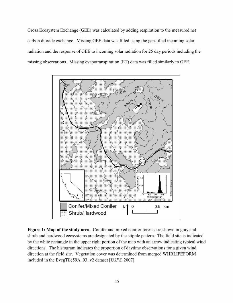
Figure 1: Map of the study area. Conifer and mixed conifer forests are shown in gray and shrub and hardwood ecosystems are designated by the stipple pattern. The field site is indicated by the white rectangle in the upper right portion of the map with an arrow indicating typical wind directions. The histogram indicates the proportion of daytime observations for a given wind direction at the field site. Vegetation cover was determined from merged WHRLIFEFORM included in the EvegTile59A_03_v2 dataset [USFS, 2007].

N

41

We determined the eddy covariance energy budget closure based on the change in energy

stored in the top 2m of soil, the latent heat flux, and the sensible heat flux. Energy storage in the

soil was determined every half hour at 5 depths by multiplying the change in temperature

measured at 5, 10, 25, 100, and 200 cm by the heat capacity of soil (including the water and

mineral fractions and assuming a 1.05 g cm-3 soil bulk density [Vargas and Allen, 2008]). The

total amount of energy stored in the top 2 m of soil was determined by summing the depth

weighted change in energy storage over the 2 m soil profile. Latent heat, sensible heat, and the

energy stored in the top 2 m of soil accounted for 65% of net radiation. We adjusted the carbon

dioxide and water vapor fluxes to account for this lack of energy budget closure [Twine et al.,

2000].

We determined the short-term half hourly response of GEE to incoming solar radiation

(K), temperature (T), and vapor pressure deficit (VPD). The forest had evergreen and deciduous

components. To minimize the confounding effect of changing leaf area and soil moisture stress

on the response of GEE to K, T, and VPD, we selected observations from two time periods with

consistent phenology and minimal soil moisture stress: Jan-May in 2007-2009 and Jul-Aug in

2008-2009. We determined the GEE response to light for these two periods based on

observations that were minimally impacted by T (T >8oC) and VPD (VPD < 2 kPa). We

determined GEE response to T and VPD using high light observations (K > 500 W m-2) from the

same time periods. We excluded T limiting observations (T <8oC) to determine the GEE

response to VPD. We excluded VPD limiting observations (VPD > 2kPa) to determine the GEE

response to T. Observations were binned and Jul-Aug GEE was homogenized with Jan-May

GEE by dividing the Jul-Aug observations by the ratio of light saturating Jul-Aug GEE to light

saturating Jan-May GEE.

42

Matric Potential and Soil Moisture

Soil matric potential (ψs, Campbell Scientific; CS229) was measured every 30 min at 5,

10, 25, 100, and 200 centimeters depths. Probes at 5, 10, and 25 centimeter depths were situated

in a backfilled ~4 cm diameter hole. Probes at 100 and 200 centimeter depths were situated in a

second backfilled hole. The holes were dug with a soil auger and refilled with the original soil

from each depth, such that the soil depth profile was preserved. The soil matric potential sensors

measured the change in temperature (δT) that resulted from applying a fixed current to a heating

element in the sensor. We related δT to ψs following [Flint et al., 2002], which requires sensor

specific measures of δT when the sensor is completely dry and completely saturated. We

measured a dry δT in the lab for each sensor prior to installation (refer to Campbell Scientific

manual), but field observed δTs exceeded the values produced in the lab. We, therefore, used the

greatest δT observed in the field to estimate the dry δT and the smallest δT observed in the field

to estimate the wet δT for each sensor. We scaled the resultant ψs from 0 to –10 MPa to produce

a relative measurement of ψs over a plausible range of ψs values.

We measured volumetric soil moisture in the top 30 cm of soil (Campbell Scientific;

CS616). We determined an empirical relationship between the depth weighted five, ten, and

twenty-five cm depth ψs and measured soil moisture in the top 30cm. We then applied the

empirical relationship to ψs measured in deeper soils to calculate the soil moisture storage in the

top 2m of soil. We determined the total amount of extractable water in the top two meters of soil

by taking the difference of the maximum volumetric water content and the minimum volumetric

water content.

The relationship between ψs and volumetric water storage did not rely on our ψs scaling

approach. Scaling ψs to -1000 MPa instead of -10 MPa changed the calculated soil water storage

43

by less than 5% over the 2 m soil profile. Measurements of soil texture indicated no change over

the 2 m profile supporting our assumption that the relationship of ψs and volumetric water

storage was consistent over the 2 m depth profile.

Forest Inventory

We established a 2-ha plot with an embedded a 0.1 ha plot in the eddy covariance

footprint. We recorded the diameter at breast height (DBH; 1.37 m) of all trees with a DBH

greater than 50 cm DBH in the 2 ha plot, and the DBH of all trees with a DBH in the 0.1 ha plot.

Leaf Area

We measured the leaf area index (LAI) 8 times during 2009 (Licor LAI-2000). Each LAI

measurement was made shortly after sunrise and consisted of 10 spot measurements along the

centerline of the inventory plot. We extrapolated LAI over three years using an empirical

relationship between the LAI-2000 observations and the local MODIS EVI pixel (LAI = 5.0724

* EVI + 0.0416; r2 = 0.68; EVI downloaded March 2010 from http://daac.ornl.gov/; MODIS

product was MOD13Q1 Collection 5).

Leaf-level gas exchange

We selected 5 to 9 trees of each Oak, Pine, and Fir species in the tower footprint for

intensive leaf level measurements in 2009. This sample of trees spanned the dominant species,

size classes, and local topographic gradient. We measured carbon assimilation (Amax) on the

most recent fully expanded leaves of each focus tree using a Licor 6400 portable photosynthesis

44

system. Measurements were made within 2.5 hours of solar noon on freshly clipped and non-

clipped branches. Clipping branches impacted mean leaf gas exchanges by less than 10%. We

did not clip Black Oak branches for leaf gas measurements. Chamber carbon dioxide mixing

ratio was controlled at 380 ppm and chamber photon flux density was controlled at 1000 µmol

m-2 s-1. Temperature and humidity varied with ambient conditions. Several of the species had

needle leaves. We inserted leaves into the chamber to minimize needle overlap and minimize

chamber leaks. We calculated leaf gas exchange using the projected leaf area within the

chamber.

We calculated a forest weighted Amax by 1) averaging Amax for each species, 2)

calculating a species weighted Amax over the forest (Amax, weighted) by summing the product of

each species Amax and the species fraction basal area normalized to one for all non-dormant

species, and 3) multiplying the forest weighted Amax and LAI. The forest weighted Amax was

calculated by: GEEmax, leaf = Amax, weighted * LAI(EVI)).

Water Potential: We measured predawn (ψpd) and midday water potentials (ψmd) on focal trees

using a Scholander pressure chamber. Predawn water potentials were measured on 1-2 twigs

from each tree. Samples were clipped two to three hours before sunrise, sealed in plastic bags,

stored in a cooler, and analyzed within two hours. Midday water potentials were measured on

one twig from each tree. Midday measurements were made immediately after clipping.

45

3.2.3 Calculations and Data Analysis

We calculated a potential GEE (GEEpotential) using incoming solar radiation (K),

temperature (T), and evaporative demand (VPD):

GEEpotential = Tscaler* Vscaler* GEE(K)

Tscaler is a temperature scalar determined by normalizing the GEE response to T, Vscaler is a

VPD scalar determined by normalizing the GEE response to VPD, and GEE(K) is GEE

determined from incoming solar radiation. GEE(K) is calculated every half hour from Oct. 1 to

June 10 (winter) using gap-filled K and the GEE response to light generated from observations

between Jan-May. GEE(K) was determined from June 10 to Sept. 30 (summer) using gap-filled

K and the GEE response to light generated from the Jul-Aug. GEE(K) was scaled by T and

VPD. This approach compared well with observed GEE (GEEpotential = 0.72 * observed GEE +

0.90; r2 =0.68; p < 0.01). The effect of T on GEE was determined by Σ GEE (K) - Σ T0-1 * GEE

(K). The effect of VPD on GEE was determined by Σ GEE (K) - Σ V0-1 * GEE (K).

We calculated the Amax-weighted day of the year (DOYA) by Σ(day of the year * Amax)/

Σ(Amax) for the water year. We calculated the TGEE by Σ(T * GEE)/ Σ(GEE).

We determined the difference between multiple groups or years using a one-way analysis

of variance. We determined the difference between slopes using analysis of covariance.

Reported confidence intervals are 95% CI unless otherwise stated.

46

3.3 Results

3.3.1 Forest Composition

The mixed conifer forest was located just above the shrubland to conifer forest ecotone

(Fig 1). The forest was composed of Oak and Pine species (Table 1). Two oaks composed the

largest fraction of total basal area: Quercus kelloggii, a deciduous oak, and Q. chrysolepis, an

evergreen oak. Four pine species composed the second largest fraction of total basal area: Pinus

lambertiana, P. Coulteri, P. ponderosa, and scattered P. jeffreyi. Calocedrus decurrens and a

limited number of Abies concolor also occurred within the tower footprint. There was a sparse

shrub understory of Ceanothus spp. and Arctostapholous spp. The site experienced substantial

tree mortality in the early 1990s and again in the early 2000s [Savage, 1994; Walker, 2006] and

many dead conifer snags remained standing.

Species Density (trees ha-1)

BA (m2 ha-1)

Plant Function Type

Abies concolor 10 0.0053 Evergreen conifer

Pinus lambertiana 252.5 4.80 Evergreen conifer

P. coulteri, ponderosa, and jeffreyi (yellow)

153 6.59 Evergreen conifer

Calocedrus decurrens 298.5 12.5 Evergreen conifer

Quercus chrysolepis 212 5.90 Evergreen broadleaf

Q. kelloggii 145.5 10.29 Deciduous broadleaf

Total 1071.5 40.09 ---

Table 1: Tree density, basal area, and plant functional type. Density (stand density; tree per hectare) and basal area (BA; m2 of tree per hectare) of dominant vegetation measured at the site. Plant Functional Type indicates the species’ plant functional type.

3.3.2 Weather

The local climate was Mediterranean, with most precipitation falling from October to

May (Fig. 2). Temperature was highest from June to September and the last day of frost ranged

47

from mid-April through May (Table 3). Hot and dry summers resulted in increased midday

VPDs, which averaged near two kPa for the entire summer. Mean summer temperature and

VPD varied little from year to year.

Figure 2: Environmental data time series at site. a) Daily mean temperature (T; ºC), b) daily mean vapor pressure deficit (VPD; kPa), c) cumulative precipitation (Pcum; mm) from nearby Idyllwild, CA, and d) daily mean volumetric soil moisture (%)

The mean precipitation was obtained from the Idyllwild, CA precipitation record and was

found to be 648 +/- 256 mm from 1943 to 2010 (mean +/- stdev; http://www.wrcc.dri.edu/,

0

10

20

30

T (

o C)

0

1

2

3

4

VP

D (

kPa)

0

200

400

600

Pcu

m (

mm

)

Jan07 Jan08 Jan09 Jan10 Jan110

10

20

SM

(%

)

Date

a)

b)

c)

d)

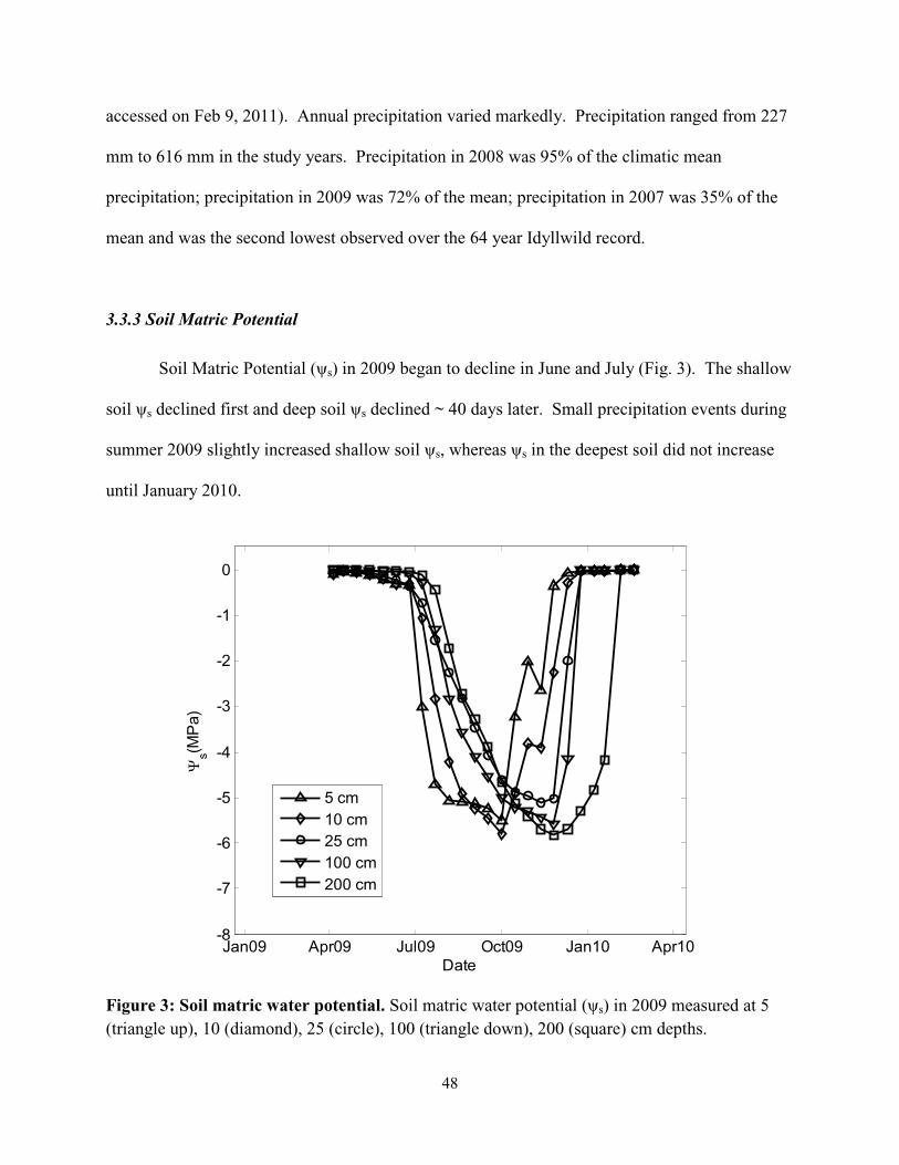
48

accessed on Feb 9, 2011). Annual precipitation varied markedly. Precipitation ranged from 227

mm to 616 mm in the study years. Precipitation in 2008 was 95% of the climatic mean

precipitation; precipitation in 2009 was 72% of the mean; precipitation in 2007 was 35% of the

mean and was the second lowest observed over the 64 year Idyllwild record.

3.3.3 Soil Matric Potential

Soil Matric Potential (ψs) in 2009 began to decline in June and July (Fig. 3). The shallow

soil ψs declined first and deep soil ψs declined ~ 40 days later. Small precipitation events during

summer 2009 slightly increased shallow soil ψs, whereas ψs in the deepest soil did not increase

until January 2010.

Figure 3: Soil matric water potential. Soil matric water potential (ψs) in 2009 measured at 5 (triangle up), 10 (diamond), 25 (circle), 100 (triangle down), 200 (square) cm depths.

Jan09 Apr09 Jul09 Oct09 Jan10 Apr10-8

-7

-6

-5

-4

-3

-2

-1

0

Date

Ψs(M

Pa)

5 cm10 cm25 cm100 cm200 cm

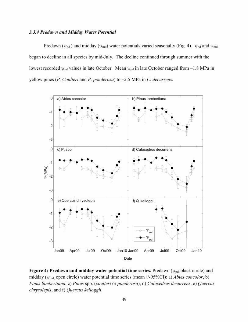
49

3.3.4 Predawn and Midday Water Potential

Predawn (ψpd ) and midday (ψmd) water potentials varied seasonally (Fig. 4). ψpd and ψmd

began to decline in all species by mid-July. The decline continued through summer with the

lowest recorded ψpd values in late October. Mean ψpd in late October ranged from –1.8 MPa in

yellow pines (P. Coulteri and P. ponderosa) to –2.5 MPa in C. decurrens.

Figure 4: Predawn and midday water potential time series. Predawn (ψpd; black circle) and midday (ψmd, open circle) water potential time series (mean+/-95%CI): a) Abies concolor, b) Pinus lambertiana, c) Pinus spp. (coulteri or ponderosa), d) Calocedrus decurrens, e) Quercus chrysolepis, and f) Quercus kelloggii.

-3

-2

-1

0

-3

-2

-1

0

Ψ(M

Pa)

Jan09 Apr09 Jul09 Oct09 Jan10

-3

-2

-1

0


Date

Ψmd

Ψpd

a) Abies concolor b) Pinus lambertiana

c) P. spp d) Calocedrus decurrens

e) Quercus chrysolepis f) Q. kelloggii

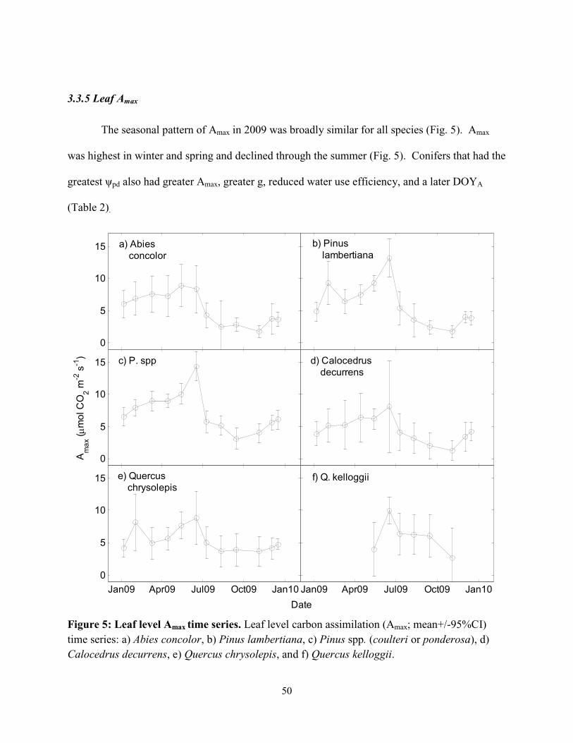
50

3.3.5 Leaf Amax

The seasonal pattern of Amax in 2009 was broadly similar for all species (Fig. 5). Amax

was highest in winter and spring and declined through the summer (Fig. 5). Conifers that had the

greatest ψpd also had greater Amax, greater g, reduced water use efficiency, and a later DOYA

(Table 2).

Figure 5: Leaf level Amax time series. Leaf level carbon assimilation (Amax; mean+/-95%CI) time series: a) Abies concolor, b) Pinus lambertiana, c) Pinus spp. (coulteri or ponderosa), d) Calocedrus decurrens, e) Quercus chrysolepis, and f) Quercus kelloggii.

0

5

10

15

0

5

10

15

Am

ax ( µ

mol

CO

2 m-2

s-1

)


5

10

15


Date

b) Pinus lambertiana

c) P. spp d) Calocedrus decurrens

f) Q. kelloggiie) Quercus chrysolepis

a) Abies concolor

51

Table 2: Conifer leaf gas exchange. Ψ group indicates the relative range of annual conifer tree Ψpd and n indicates the number of trees in each bin. Ψpd (MPa) is the range of annual mean predawn water potential. Amax (µmol CO2 m

-2 s-1) is the mean (+/- 95%CI) of each conifer’s mean carbon assimilation measurements. g (mol H2O m-2 s-1) is the mean (+/- 95%CI) of each conifer’s mean stomatal measurements. A g-1

(µmol CO2 mol H2O-1) is the mean (+/- 95%CI) of

each conifer’s mean water use efficiency. DOYA (day) is the Amax-weighted day of year for all leaf gas measurements. Letters indicate difference between groups.

3.3.6 GEE

The forest remained photosynthetically active the entire year (Fig. 6; Fig. 7). Leaf level

Amax measurements yielded a similar seasonal pattern to the seasonal pattern of light saturated

GEE measured by eddy covariance (GEEmax; Fig. 6). The agreement confirmed a seasonal

pattern in 2009 characterized by increased rates of carbon uptake from January through June, a

peak in GEE near July, and a decline in GEE through October.

Mean 60 day binned GEEmax, reached ~11 µmol CO2 m-2 s-1 in early July in 2008 and

2009 and in early May in 2007. The lowest 60 day binned GEEmax occurred late in the 2007

water year and early 2008 water year when GEEmax declined to near 4 µmol CO2 m-2 s-1 (Fig. 7).

GEE during the summer of 2007 was 64% of the year’s average annual GEE (Table 3). This was

lower than in 2008 or 2009, when GEE during the summer was 116% and 96% of the year’s

average annual GEE respectively (Table 3).

Ψ group Ψ range (MPa)

Amax (µmol CO2 m

-2 s-1) g (mol

H2O m-2 s-1) A g-1 (µmol CO2

mol H2O-1)

DOYA

(day) Low (n=10) -0.86 to -1.00 6.84 (0.94)a 0.086 (0.017)a 93 (8)a Apr 10a

Medium (n=10) -1.00 to -1.14 6.07 (0.82)a,b 0.062 (0.008)b 107 (7)b Apr 7a,b

High (n=9) -1.14 to -1.78 5.19 (0.97)b 0.053 (0.010)b 107 (9)b Mar 31b

52

Figure 6: Amax, leaf area, and GEE time series. Time series in 2009 of: a) carbon assimilation (Amax (µmol CO2 m

-2 s-1); mean +/- standard error) weighted by the proportion of non-dormant species basal area, b) LAI (m2 m-2), and c) the product of weighted Amax and LAI (black square) and daily mean eddy covariance GEE (gray) for observations with incoming solar radiation greater than 500 W m-2

.

0

5

10

15A

ma

x( µ

mol

CO

2 m

-2 s

-1)

1

1.5

2

LAI

(m2 m

-2)


10

20

30

GE

E( µ

mol

CO

2 m

-2 s

-1)

DOY

c)

b)

a)

53

Figure 7: GEE time series for 2007, 2008, and 2009. Sixty day mean Gross Ecosystem Exchange (GEE (µmol CO2 m

-2 s-1)) for observations with incoming solar radiation greater than 500 W m-2 for 2007, 2008, and 2009.

Table 3: Ecosystem level properties. P (mm) is the annual Idyllwild, CA precipitation measured from Oct 1 to Sep 30. T (oC) is the mean annual air temperature measured at the top of the eddy covariance tower. Ts (

oC) is the mean summer (June 10 to Sept. 30) air temperature measured at the tower. TGEE (

oC) is the GEE-weighted mean annual air temperature. VPDs is the mean summer VPD. GEEs (%) is ratio of mean Gross Ecosystem Exchange (GEE) measured during the summer to the mean annual GEE. Dfrost (day) is the last day of the year that the temperature was below 0 oC. LAIpeak (day) was the day of the year that peak LAI occurred. LAIs (m

2 m-2) was mean summer LAI.

Oct Jan Apr Jul Oct0

2

4

6

8

10

12

14

16G

EE

( µm

ol C

O2 m

-2 s

-1)

Month

200720082009

= mean 2-sided 95% CI

Year P(mm) T (oC) Ts (oC) TGEE(oC) VPDs(kPa) GEEs (%) Dfrost(day) LAIpeak(day) LAIs(m

2 m-2)

2007 227 13.36 20.91 15.09 1.96 64% 111 161 1.73

2008 616 13.06 21.40 16.65 1.92 116% 146 209 1.91

2009 464 13.74 20.51 16.16 1.90 96% 106 161 1.78

54

3.3.7 Climate constraints

GEE dropped when temperatures decreased below 8ºC (Fig. 8) and also with increased

VPD (Fig. 9). High VPD placed an overall greater control on GEE than low temperature (Table

4). High VPD during the summer reduced the annual sum of calculated GEE(K) by 170 to 186

gC m-2 yr-1 (13 to 14% of GEE(K); Table 4). These reductions were greater than direct

reductions in GEE due to cold temperature, which ranged from 40 to 58 gC m-2 yr-1 (3 to 4% of

GEE(K); Table 4).

Figure 8: GEE response to temperature. Gross Ecosystem Exchange (GEE(µmol CO2 m-2 s-1);

mean +/- 95% CI) response to temperature (T (oC)) for observations with vapor pressure deficits less than 2 kPa and for periods between January-May (black triangle) and July-August (open triangle). July-August observations were divided by the ratio of mean light saturating summer GEE to mean light saturating winter GEE.

-5 0 5 10 15 20 25 300

2

4

6

8

10

12

T ( oC )

GE

E ( µ

mol

CO

2 m-2

s-1

)

Jan-MayJul-Aug

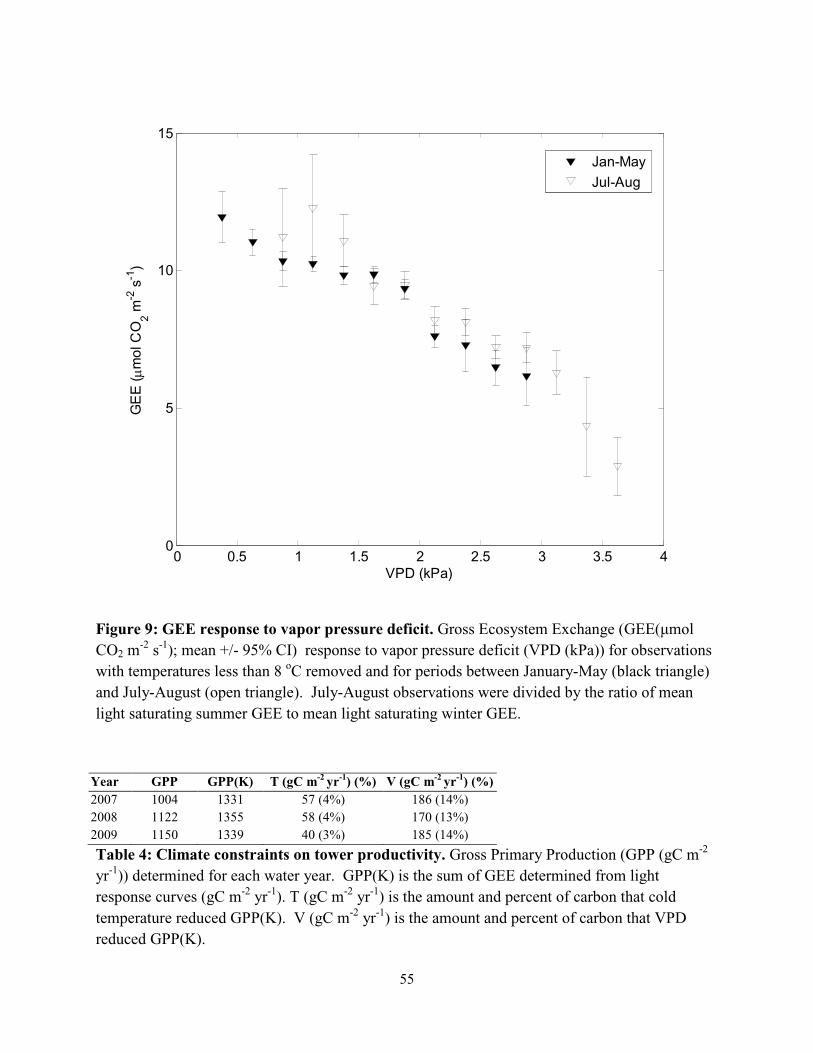
55

Figure 9: GEE response to vapor pressure deficit. Gross Ecosystem Exchange (GEE(µmol CO2 m

-2 s-1); mean +/- 95% CI) response to vapor pressure deficit (VPD (kPa)) for observations with temperatures less than 8 oC removed and for periods between January-May (black triangle) and July-August (open triangle). July-August observations were divided by the ratio of mean light saturating summer GEE to mean light saturating winter GEE.

Year GPP GPP(K) T (gC m-2 yr-1) (%) V (gC m-2 yr-1) (%) 2007 1004 1331 57 (4%) 186 (14%) 2008 1122 1355 58 (4%) 170 (13%) 2009 1150 1339 40 (3%) 185 (14%)

Table 4: Climate constraints on tower productivity. Gross Primary Production (GPP (gC m-2 yr-1)) determined for each water year. GPP(K) is the sum of GEE determined from light response curves (gC m-2 yr-1). T (gC m-2 yr-1) is the amount and percent of carbon that cold temperature reduced GPP(K). V (gC m-2 yr-1) is the amount and percent of carbon that VPD reduced GPP(K).

0 0.5 1 1.5 2 2.5 3 3.5 40

5

10

15G

EE

( µm

ol C

O2 m

-2 s

-1)

VPD (kPa)

Jan-MayJul-Aug

56

3.3.8 Soil water balance:

Total plant extractible water in the top 2 m of soil (S0-200) was 226 mm. The initial

decline in S0-200 in 2009 coincided closely with the last large rainfall of the water year. The

initial S0-200 decline was similar to evapotranspiration (ET). ET continued after S0-200 showed

nearly no change. S0-200 declined by ~200 mm from April 20 to Sept. 30 (Fig. 10). ET was

greater than 400 mm of water over the same period exceeding the sum of S0-200 and summer

precipitation by over 200 mm.

Figure 10: 2009 water balance. Water balance in 2009: Storage top 2m is water stored in the top 2 m of soil (bold line). ΣET is the cumulative evapotranspiration measured at the eddy covariance tower (dashed line). Σ P is cumulative precipitation (mm; solid line).

Jan09 Apr09 Jul09 Oct09 Jan10-300

-200

-100

0

100

200

300

400

500

mm

Wat

er

Date

Storage top 2m

Σ ET

Σ P

Loss

Input

57

Averaged water year annual ET was 602mm over the three study years, which exceeded

the 436 mm mean precipitation for the same period. Averaged annual ET was 93% of the long-

term mean precipitation in Idyllwild, CA. ET was lowest in 2007 when 481 mm of water

evaporated. ET was 657 mm in 2008 and 668 mm in 2009.

3.4 Discussion

3.4.1 Leaf level responses to drought stress

The Mediterranean climate drove a clear seasonal pattern of leaf gas exchange; species’

Amax declined during the summer (Fig. 5). The observed magnitude of Amax was similar to

previously reported Amax for semiarid conifer and oak vegetation [Kolb and Stone, 2000; Pavlik

and Barbour, 1991], with the exception of Black Oak where previous reports found greater Amax

in the nearby San Bernardino Mountains, CA [Grulke et al., 2005].

ψpd measurements indicated a decline in plant water access during the seasonal summer

drought (Fig. 4). Soil water availability began to decline in July, coincident with the onset of

summer drought, and was reduced over the entire summer. The decline in ψpd was both longer

and more extreme than that measured in the mid and upper montane forests in the Sierra Nevada

[Royce and Barbour, 2001].

We pooled all conifer species into three groups based on their annual ψpd. Conifers with

the least negative ψpd had greater annual mean Amax and annual stomatal conductance, g (Table

2). Trees with improved soil water availability also had a later DOYA, a pattern that was driven

primarily by increased Amax in spring and early summer. Reduced water use efficiency in the

least water stressed trees was most pronounced in winter months and water use efficiency

58

converged to similar values in summer. Several of the conifers that were in the least water

stressed group were located near a local topographic low area in the plot. Water may have

flowed toward this local low and ths location may have had deeper soils. These data indicated

that conifers rooted in more favorable sites have increased carbon uptake at the expense of

greater overall water loss.

3.4.2 What are the environmental controls on forest productivity?

Cold temperature, high evaporative demand, and reduced soil water availability all

limited ecosystem GEE. Of the three, the direct impacts of cold temperature had a relatively

minor impact on GEE while high evaporative demand led to consistently large reductions in

GEE each year (Table 4) and reductions in GEE due to soil water limitations were most apparent

in the 2007 drought year (Table 3; Fig 7).

Cold Temperature

Cold temperature limited productivity in two ways: 1) direct constraint on evergreen

photosynthesis and 2) indirectly through black oak phenology.

Direct constraints on GEE due to cold temperature occurred below ~8oC (Fig. 8). Low

temperatures only occurred during non-summer periods (Fig. 2), which were characterized by

large temperature variability, with occasional cold events below 8oC that led to brief constraints

on GEE. Overall, cold constraints on GPP were minor, resulting a decreased carbon uptake by

~40 to 58 gC m2 yr-1 or 3 to 4% (Table 4).

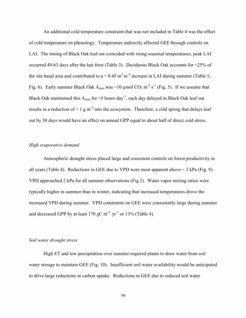
59

An additional cold temperature constraint that was not included in Table 4 was the effect

of cold temperature on phenology. Temperature indirectly affected GEE through controls on

LAI. The timing of Black Oak leaf out coincided with rising seasonal temperatures; peak LAI

occurred 49-63 days after the last frost (Table 3). Deciduous Black Oak accounts for ~25% of

the site basal area and contributed to a ~ 0.45 m2 m-2 increase in LAI during summer (Table 1;

Fig. 6). Early summer Black Oak Amax was ~10 µmol CO2 m-2 s-1 (Fig. 5). If we assume that

Black Oak maintained this Amax for ~5 hours day-1, each day delayed in Black Oak leaf out

results in a reduction of ~ 1 g m-2 into the ecosystem. Therefore, a cold spring that delays leaf

out by 30 days would have an effect on annual GPP equal to about half of direct cold stress.

High evaporative demand

Atmospheric drought stress placed large and consistent controls on forest productivity in

all years (Table 4). Reductions in GEE due to VPD were most apparent above ~ 2 kPa (Fig. 9).

VPD approached 2 kPa for all summer observations (Fig 2). Water vapor mixing ratios were

typically higher in summer than in winter, indicating that increased temperatures drove the

increased VPD during summer. VPD constraints on GEE were consistently large during summer

and decreased GPP by at least 170 gC m-2 yr-1 or 13% (Table 4).

Soil water drought stress

High ET and low precipitation over summer required plants to draw water from soil

water storage to maintain GEE (Fig. 10). Insufficient soil water availability would be anticipated

to drive large reductions in carbon uptake. Reductions in GEE due to reduced soil water

60

availability did not appear to be great in 2008 or 2009 as high rates of carbon uptake continued

late into the water year.

Soil drought stress appeared to be large in 2007. We estimated that plant available water,

S0-200, in the top 2 m of soil stored ~226 mm of water. Precipitation in 2007 was 227 mm and

nearly equaled S0-200; the soil in 2007 was probably not recharged with water below 2 m.

Reductions in GEE during the summer of 2007 (Table 3; Fig 7) were likely driven by this

reduced soil water availability. According to our potential GEE calculation, reductions in GEE

due to VPD were only slightly greater in 2007 than in other years (Table 4) and the difference

was insufficient to account for the large reductions in GEE observed in the 2007 summer

compared with GEE observed in the 2008 or 2009 summers. The reduction in GEE owing to

reduced soil water availability in 2007 indicates that production in this forest may decline when

winter precipitation is low and soil water pools are not recharged over the wet winter period.

3.4.3 How does a semiarid forest survive at the warm and dry edge of its range?

Two attributes of this ecosystem allow mixed conifer forests to survive at their low

elevation forest ecotone: 1) GEE remains high at low temperatures and 2) vegetation accesses

water stored in deep soils. These attributes extend this forest’s growing season over the entire

year, including a cool wet winter and a warm dry summer.

Low Temperature GEE

This mixed conifer forest maintained large carbon uptake at low temperatures. GEE

response to temperature showed high carbon uptake over a wide breadth of temperatures with

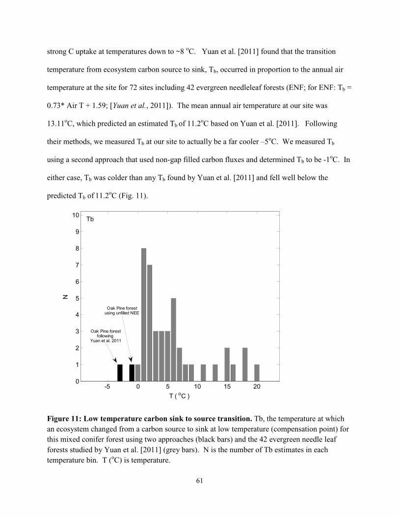
61

strong C uptake at temperatures down to ~8 oC. Yuan et al. [2011] found that the transition

temperature from ecosystem carbon source to sink, Tb, occurred in proportion to the annual air

temperature at the site for 72 sites including 42 evergreen needleleaf forests (ENF; for ENF: Tb =

0.73* Air T + 1.59; [Yuan et al., 2011]). The mean annual air temperature at our site was

13.11oC, which predicted an estimated Tb of 11.2oC based on Yuan et al. [2011]. Following

their methods, we measured Tb at our site to actually be a far cooler –5oC. We measured Tb

using a second approach that used non-gap filled carbon fluxes and determined Tb to be -1oC. In

either case, Tb was colder than any Tb found by Yuan et al. [2011] and fell well below the

predicted Tb of 11.2oC (Fig. 11).

Figure 11: Low temperature carbon sink to source transition. Tb, the temperature at which an ecosystem changed from a carbon source to sink at low temperature (compensation point) for this mixed conifer forest using two approaches (black bars) and the 42 evergreen needle leaf forests studied by Yuan et al. [2011] (grey bars). N is the number of Tb estimates in each temperature bin. T (oC) is temperature.

-5 0 5 10 15 200

1

2

3

4

5

6

7

8

9

10

N

T ( oC )

Tb

Oak Pine forestfollowing

Yuan et al. 2011

Oak Pine forestusing unfilled NEE

62

Globally, most photosynthesis occurs when leaf temperatures are ~ 21oC [Helliker and

Richter, 2008]. Mean GEE-weighted temperatures, TGEE, of 15oC to 17oC indicated that either

most photosynthesis occurred at lower leaf temperatures than typical or the leaves in the canopy

warmed through strong thermal adjustment. Reduced CO2 uptake in the late summer when

temperatures were still high reduced TGEE. TGEE in the 2007 drought year was lower than TGEE in

2008 or 2009.

Infrequently cold but not too cold winter temperatures may have created an environment

for high GEE at low temperatures. The lowest recorded half hourly temperature with

K > 0 W m –2 was -6.8ºC and freezing temperatures did not last very long. This forest was well

adapted to maintain photosynthesis at cold temperatures just above freezing. We hypothesize

that ecosystems with the coldest periods of the year just above freezing will be the most cold

adapted ecosystems (eg. [Waring and Franklin, 1979]). Ecosystems located in warmer

environments will favor warm adapted species and ecosystem with a large number of days below

freezing may favor cold dormant species and a shift in the growing season to warmer periods of

the year.

Deep soil water access

Vegetation relied on stored water to support productivity over the dry summer (Fig. 10).

Precipitation during the summer was insufficient to meet high evaporative demands. Most

precipitation in 2009, for example, fell between October and April with small convective

rainstorms contributing little precipitation over the remaining water year; small rainstorms added

7 mm of water between days 110 and 273 in 2009 (excluding interception losses). Water for

63

evaporation must have come from water stored in the soil. ET exceeded the sum of water stored

in the top two meters of soil and summer precipitation by ~200 mm and ET continued after Stwo

showed only small changes (Fig. 10). These patterns indicated that vegetation accessed water

stored deeper than 2m in the soil and may have extracted water at depth exceeding ~4 m.

Vegetation in mixed conifer forests is deeply rooted, which allows access to water stored

in deep soils and ameliorates late summer vegetation drought stress. Soils at the field site,

however, did not appear to be as deep, nor were they indicated as deep on maps. Rather, trees

may have accessed water stored in underlying fractured bedrock. Arkley [1981] performed a

water balance in the nearby San Bernardino Mountains and concluded that “highly productive

forests of California survive through the frequent dry summers by using water stored deep in the

decomposed granite or fractured rock substrate.” Water stored in bedrock contributed at least

70% of water used during the growing season in low elevation Sierra Nevada forests [Witty et

al., 2003].

Soil water storage in deep soils may also act to buffer the large interannual fluctuations in

precipitation. Severe droughts similar to the 2007 drought may exceed soil water storage

buffering capacity and lead to the large reductions in GEE like we observed in 2007 (Table 3).

3.4.4 Are low elevation mixed conifer forests vulnerable to climate change?

Climate change is predicted to increase California statewide temperature [Cayan et al.,

2008]. Precipitation projections are less certain; earlier models indicated possible increases, but

more recent model runs have indicated possible reductions [Seager and Vecchi, 2010].

64

In principle, warming associated with climate change could help this forest by reducing

cold stress, or it could hurt this forest by increasing drought stress. Warmer winters would

reduce cold stress but the anticipated benefit would be small because cold stress is already small.

Warmer summers may have a greater impact on production in this forest. Increased

temperatures will increase VPD if there is not a sufficiently large increase in absolute humidity.

High VPDs exert strong controls on GEE. To assess how warming may affect this forest, we

estimated how much a daily 3 oC temperature increase would affect GEEpotential. Reductions in

cold stress increased carbon uptake by ~31 gC m-2 yr-1, but the effect of increased VPD

(assuming the same vapor pressure) led to a reduction of ~115 gC m-2 yr-1, driving an overall

decrease in gross production.

Increases in mean precipitation may have a small benefit by increasing water availability.

However, these forests are deeply rooted and do not appear to be strongly water limited in

typical years. Reductions in mean precipitation or an increase in precipitation variability that

leads to more drought years may result in large reductions in carbon uptake if precipitation fails

to recharge soil water storage. In a severe drought, even deeply rooted vegetation may not be

able to access water stored in the soil. For example, below average precipitation in 2007 reduced

summer GEE markedly. Several consecutive years of drought may drive sustained reductions in

GEE, which may have implications for vegetation health [McDowell et al., 2008]. Tree

mortality in the San Jacinto Mountains has occurred with prolonged droughts over the past 100

years (Chapter 2) and, recently, high tree mortality in the San Jacinto Mountains followed severe

and prolonged droughts, indicating that these forests are vulnerable to reductions in precipitation

[Savage, 1994; Walker, 2006].

65

Overall, this forest appears most vulnerable to increases in VPD and reductions in

precipitation that may accompany climate change. Increased certainty in the response of low

elevation forest productivity to climate change would benefit from improved estimates of: 1)

regional climate scenarios and 2) plant available water, including landscape level estimates of

soil water holding capacity and rooting depth of vegetation.

66

Chapter 4: Can the short-term meteorological controls

on canopy photosynthesis explain the long-term

relationship between climate and vegetation along an

elevation gradient?

4.1 Introduction

Elevational climate patterns and vegetation are well correlated in Western US mountains.

Vegetation distributions in the Sierra Nevada mountains in central California and the Peninsular

Range in Southern California are strongly correlated with elevational patterns in climate

[Hamilton, 1983; Hanawalt and Whittaker, 1976; Kelly and Goulden, 2008; Urban et al., 2000].

Net plant production in Arizona’s Santa Catalina Mountains increases with increasing

precipitation and decreasing temperature at higher elevations [Whittaker and Niering, 1975].

67

Despite these established correlations, the means by which climate shapes vegetation patterns is

unclear.

We consider the relationship between climate and gross primary production.

Meteorological controls of temperature and water availability place controls on the short-term

variability in ecosystem production [Law et al., 2002], and the cumulative effects of short-term

ecosystem production may directly determine the long-term climate-equilibrated pattern of plant

production. Additional controls, however, influence the long-term pattern in production through

processes impacting leaf area, vegetation structure, species composition, disturbance, and soil

properties [Chapin et al., 2002].

We determined how the short-term controls of temperature and water availability would

be expected to shape the pattern of production with elevation in the San Jacinto Mountains, CA,

and whether those relationships drive the long-term pattern of production with elevation. We

used gross primary production (GPP), the total carbon uptake by an ecosystem, as our measure

of production. We focused on five questions: 1) How does canopy photosynthesis respond to

short-term changes in light, temperature, and water availability? 2) How do temperature and

water availability vary with elevation? 3) How does this elevational pattern of temperature and

water availability affect canopy photosynthesis with elevation? 4) How does the long-term,

climate-equilibrated pattern of GPP vary with elevation? 5) Can the short-term meteorological

controls on canopy gas exchange explain the observed long-term relationship between climate

and GPP?

We established an elevation transect on the western slope of the San Jacinto Mountains in

Southern California (33o 49’ N, 116o 46’ W). We determined the physiological responses of a

68

mid-elevation forest to short-term meteorological controls of light, temperature, and water

availability. We then extended these physiological responses to the entire montane elevation

gradient based on the relationship between meteorology and elevation. Finally, we compared

this short-term control derived GPP (GPPshort) with the observed long-term, climate-equilibrated

pattern in GPP (GPPlong). Our approach was empirical and based on an extrapolation of the

physiological responses observed at a site located midway along the elevation transect. We

implicitly assumed that ecosystems across the landscape have similar soil types, structure,

ecosystem function, and history to the central site. By making these assumptions, we were able

to consider whether short-term meteorological controls could directly shape the elevational

pattern in GPP.

4.2 Methods

4.2.1 Vegetation patterns over the elevation transect

We determined how vegetation cover varied with elevation from 1295 m to 3002 m using

300-m long belt transects at 122-m elevation intervals (Chapter 2 of this dissertation). We

measured the total fraction cover (Σ projected vegetation crown onto a one dimensional sampling

transect / length of the sampling transect) for all woody vegetation. We then calculated the

normalized cover for four vegetation groups (normalized cover = Σ vegetation group cover (m)

/Σ total vegetation cover (m)): Chaparral shrubs, Oaks, Mid-elevation Pines and Firs, and

Subalpine conifers. Chaparral shrubs were reported by Adenostoma fasciculatum,

Arctostaphylos glandulosa, and A. glauca; Oaks by Quercus chrysolepis, Q. kelloggii, and Q.

wislizenii; Mid-elevation Pines and Firs by Abies concolor, Pinus coulteri, P. lambertiana, P.

ponderosa, P. jefferyi; Subalpine conifer by Pinus flexilis and P. contorta.

69

4.2.2 Short-term ecosystem level response to meteorology

We used eddy covariance techniques to measure the exchanges of carbon dioxide, water

vapor, and energy ~ 5 m above the canopy at a central site located at 1708 m ([Goulden et al.,

2006]; Ameriflux site: Southern California Climate Gradient Oak Pine Forest / US-SCf; Table

1). This site was a mixed conifer forest with a diverse mixture of evergreen shrubs, evergreen

and deciduous oak trees, evergreen conifer trees, and deciduous oak trees (Chapter 3 of this

dissertation). The latent heat flux, sensible heat flux, and energy stored in the top two meters of

soil accounted for 65% of net radiation. We adjusted the turbulent fluxes accordingly [Twine et

al., 2000]. We also measured incoming solar radiation (K) and temperature (T) at the top of the

eddy covariance tower.

Respiration was determined by extending the Net Ecosystem Exchange (NEE) light

response to darkness for 25 day periods. Half-hourly Gross Ecosystem Exchange (GEE) was

calculated by subtracting respiration from observed NEE.

We determined the response of GEE to K and T. GEE response to K was determined

from observations that were minimally impacted by temperature (8 oC < T < 22 oC) and

separated for two intervals that corresponded to shifts in ecosystem phenology (January through

May and July through August). GEE response to T was determined for bright light (K > 500 W

m-2) during the same intervals. GEE was averaged for one degree temperature bins. July-August

observations were homogenized with January-May observations by dividing the July- August

observations by the ratio of mean July-August to mean January-May high light observations.

GEE response to T was then normalized to construct a temperature scalar (T0-1).

70

We constructed continuous K and T time series at the central site by filling short data

gaps. Short data gaps were filled using interpolation (gaps <= 2.5 hours). Longer data gaps

(gaps > 2.5 hours) were filled with the corresponding mean for the time of day from a 25 day

period.

4.2.3 Transect meteorology

We determined the elevational pattern of temperature and soil water availability from

1990 to 2009 for the western slope of the San Jacinto Mountains.

Temperature

The temperature lapse was determined from radiosonde soundings at the Miramar station

(NKX; 33o 51’ 0” -117o 6’ 36” ). The Miramar radiosonde was launched ~120 km upwind of the

prevailing weather patterns twice a day from 1990 to 2009 (http://weather.uwyo.edu/upperair

/sounding.html on 9/20/2010). We linearly interpolated the radiosonde temperatures to 122-m

intervals from 853 m to 3414 m. We adjusted the 2008 water year air temperature measured at

the central site by the difference in temperature between the radiosonde temperature measured at

the central site altitude and that measured at 122-m intervals.

Precipitation

We obtained precipitation (P) records from weather stations on the western slopes of the

San Jacinto and nearby San Bernardino Mountains from the Western Regional Climate Center

(WRCC; http://www.wrcc.dri.edu accessed April 2010) and the National Climatic Data Center

71

(NCDC; http://www.ncdc.noaa.gov accessed April 2011). WRCC cooperative observer network

weather stations (COOP) records calculated mean precipitation by including years with no more

than 5 missing observations in any month of the year. Mean annual precipitation was determined

from NCDC daily precipitation records following the same approach. Precipitation records

shorter than 10 years were adjusted to the long-term mean precipitation using Idyllwild’s long-

term mean precipitation.

We normalized the precipitation elevation profile by dividing all precipitation records by

the mean precipitation above 1500 m for each mountain independently. This approach corrected

for a north to south gradient in precipitation.

Evapotranspiration

We determined evapotranspiration (ET) at 122-m intervals every 30 min using the

Penman-Monteith Equation (PM):

λv ET = (∆ (Rn-G) + ρ cp VPD ga )/(∆ + γ(1 + ga/gs))

where ET is evaporation, ∆ is the slope of saturation specific humidity with air temperature, Rn is

net radiation, G is ground heat flux, ρ is air density, cp is the specific heat capacity of air, VPD is

the vapor pressure deficit, ga is the aerodynamic conductance, gs is the surface conductance, γ is

the psychrometric constant, and λv is the latent hear of vaporization.

We adjusted Rn measured at the tower by the local elevational gradient in Rn

(Rn=0.004641*elevation(m)+109.14; [Jin et al., 2011]) and set G to zero (c.f. [Lundquist and

Loheide, 2011]). VPD is the difference between the vapor pressure and the saturation vapor

72

pressure, which, in turn, depends on temperature. The saturation vapor pressure for all

elevations was determined from the radiosonde adjusted tower temperature. We assumed the

water vapor mixing ratio was constant with elevation and set to the observation at the central site

(c.f. [Lundquist and Loheide, 2011]). Atmospheric pressure was determined by altitude

([Campbell and Norman, 1998]; c.f. [Lundquist and Loheide, 2011]). We determined ga and gs

at half-hourly intervals at the tower for the 2008 water year by inverting the PM equation and

then applied the 2008 ga and gs to all elevations and years.

Data gaps in the eddy covariance time series were caused by power failure, equipment

failure, and non-turbulent atmospheric conditions (u* < 0.30 m s-1), which led to gaps in the PM

ET. Gaps in the PM ET were filled with a relationship between PM ET and K for 25 day periods

at each elevation independently.

4.2.4 Soil water storage capacity

We estimated soil water storage for the entire San Jacinto River watershed, which

included a large part of the transect. We used a water balance approach similar to Stephenson

[1990]: Water storage change = P - ET - Runoff (R). P was determined from Idyllwild, CA

precipitation measurements from 1949 to 1990 and was adjusted for elevation. ET was

determined from PM ET and was adjusted for elevation. R was determined from historic

monthly San Jacinto River discharge during 1949 to 1990 (San Jacinto Rv + canal; ID

11069501). Rainy season P - ET (months when P exceeded PM ET) was summed over the water

year and regressed against the annual R.

73

R increased when the rainy season P - ET exceeded 315 mm (Fig. 1). We extended the

linear portion of the Rainy season P - ET vs. R curve to no discharge to determine the soil water

storage capacity (Discharge = 0.583* Surplus -184; p= 0.02; r2 = 0.62; n=8; Fig. 1). Soil water

storage was estimated as 315 mm in the San Jacinto River watershed. We assumed this soil

water storage estimate was constant at all elevations over the transect.

Figure 1: Runoff vs. P- PM ET. Rainy Season P – PM ET (mm) is the difference between precipitation (P) and the Penman-Monteith evaporation (PM ET) for periods when P exceeds PM ET. Runoff is the San Jacinto River discharge. Filled triangles are used in the regression and open triangle are the remaining years.

0 200 400 600 800 10000

50

100

150

200

250

300

350

400

Rainy Season P - PM ET (mm)

Run

off (

mm

)

Soil Water Storage

74

4.2.5 Plant water availability

Plant water availability was calculated every 30 min at 122-m intervals using a simple

bucket model. Precipitation input was driven by the daily Idyllwild, CA precipitation record

(COOPID 44211). The precipitation at each elevation was determined by multiplying Idyllwild

precipitation by the normalized elevational mean precipitation curve. Precipitation was added to

the soil water storage at the start of each day, and water removed by evapotranspiration every 30

min. Precipitation that exceeded soil water storage capacity was runoff.

Higher elevations receive more precipitation as snow [Minnich, 1986]. The Southern

California snowpack was intermittent over most elevations and persisted until June at the highest

elevations [Minnich, 2007]. Snow melt typically occurred before or near the last seasonal

rainfall, indicating that explicitly accounting for water stored in snow would not improve our

plant available water estimate.

4.2.6 GPP determined by short-term meteorological controls

We determined how meteorological controls on canopy photosynthesis affected carbon

uptake over the transect (Fig. 2). We estimated Gross Ecosystem Exchange, GEE, over the

elevation gradient every half hour as:

GEEshort = WA T0-1 GEE(K)

where GEE(K) was the GEE estimated from incoming solar radiation and a light response curve.

The January through May light response curve was used to determine GEE(K) from Oct. 1 to

June 10 and the July through August light response curve was used to determine GEE(K) from

June 10 to Sept. 30. T0-1 was the temperature scalar. WA was a binary multiplier that accounted

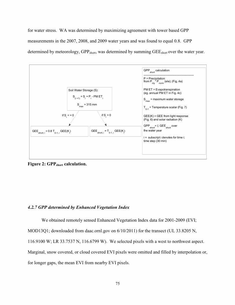
75

for water stress. WA was determined by maximizing agreement with tower based GPP

measurements in the 2007, 2008, and 2009 water years and was found to equal 0.8. GPP

determined by meteorology, GPPshort, was determined by summing GEEshort over the water year.

Figure 2: GPPshort calculation.

4.2.7 GPP determined by Enhanced Vegetation Index

We obtained remotely sensed Enhanced Vegetation Index data for 2001-2009 (EVI;

MOD13Q1; downloaded from daac.ornl.gov on 6/10/2011) for the transect (UL 33.8205 N,

116.9100 W; LR 33.7537 N, 116.6799 W). We selected pixels with a west to northwest aspect.

Marginal, snow covered, or cloud covered EVI pixels were omitted and filled by interpolation or,

for longer gaps, the mean EVI from nearby EVI pixels.

if Si > 0

GEEshort, i

= 0.8 T0-1, i

GEE(Ki) GEE

short, i = T

0-1, i GEE(K

i)

GPPshort

calculation

-------------------------------------------------------P = Precipitation from P

idy* P

norm (ele); (Fig. 4a)

PM ET = Evapotranspiration (eg. annual PM ET in Fig. 4c)

Smax

= maximum water storage

T0-1

= Temperature scalar (Fig. 7)

GEE(K) = GEE from light response (Fig. 6) and solar radiation (K)

GPPshort

= Σ GEEshort

over

the water year

i = subscript i denotes for time i;time step (30 min)

if Si < = 0

Soil Water Storage (S):

S(i +1)

= Si + P

i - PM ET

i

Smax

= 315 mm

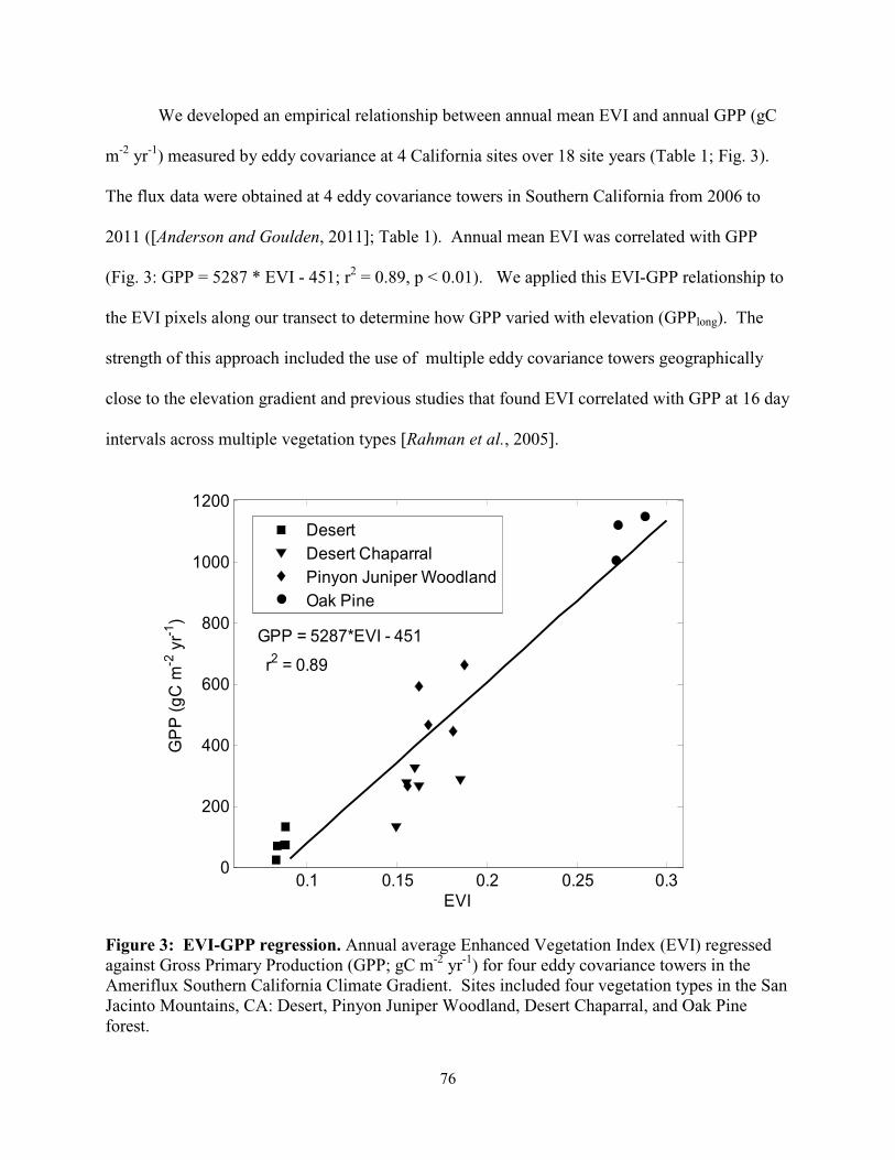
76

We developed an empirical relationship between annual mean EVI and annual GPP (gC

m-2 yr-1) measured by eddy covariance at 4 California sites over 18 site years (Table 1; Fig. 3).

The flux data were obtained at 4 eddy covariance towers in Southern California from 2006 to

2011 ([Anderson and Goulden, 2011]; Table 1). Annual mean EVI was correlated with GPP

(Fig. 3: GPP = 5287 * EVI - 451; r2 = 0.89, p < 0.01). We applied this EVI-GPP relationship to

the EVI pixels along our transect to determine how GPP varied with elevation (GPPlong). The

strength of this approach included the use of multiple eddy covariance towers geographically

close to the elevation gradient and previous studies that found EVI correlated with GPP at 16 day

intervals across multiple vegetation types [Rahman et al., 2005].

Figure 3: EVI-GPP regression. Annual average Enhanced Vegetation Index (EVI) regressed against Gross Primary Production (GPP; gC m-2 yr-1) for four eddy covariance towers in the Ameriflux Southern California Climate Gradient. Sites included four vegetation types in the San Jacinto Mountains, CA: Desert, Pinyon Juniper Woodland, Desert Chaparral, and Oak Pine forest.

0.1 0.15 0.2 0.25 0.30

200

400

600

800

1000

1200

EVI

GP

P (g

C m

-2 y

r-1)

DesertDesert ChaparralPinyon Juniper WoodlandOak Pine

GPP = 5287*EVI - 451

r2 = 0.89

77

Table 1: Site information. Sites used to determine the relationship between mean Enhanced Vegetation Index (EVI) and Gross Primary Production (GPP). These sites were part of the Ameriflux Southern California Climate Gradient (SCCG; US-SCx). The site ID and vegetation type are given. Elevation is the elevation of the tower in meters (m). Tower Site and MODIS Target are the latitude and longitude of the eddy covariance tower and corresponding EVI pixel in Degrees Minutes, and Seconds (DMS) used to develop the relationship between GPP and EVI. Years are the range of years included in the comparison.

Site ID

Vegetation Type

Elevation (m)

Tower Site (DMS)

MODIS Target (DMS)

Years

US- SCd Desert 274 33o 39’ 6” N 116o 22’ 20” W 33o 39’ 6” N 116o 22’ 27” W 2007-11

US-SCw Pinyon Juniper Woodland

1277 33o 36’ 18” N 116o 27’ 17” W 33o 35’ 18” N 116o 26’ 39” W 2007-11

US-SCc Desert Chaparral

1298 33o 36’ 36” N 116o 27’ 1” W 33o 36’ 36” N 116o 26’ 55” W 2007-11

US-SCf Oak Pine Forest

1708 33o 48’ 28” N 116o 46’ 18” W 33o 48’ 28” N 116o 26’ 25” W 2007-09

78

4.3 Results

4.3.1 Climate and meteorology

Seasonal and interannual climate

The climate in the San Jacinto Mountains is Mediterranean with mild, wet winters and

warm, dry summers. Most precipitation arrives during winter; over 80% of precipitation falls

from October to May ([WRCC]; http://www.wrcc.dri.edu accessed April 2010). Mean annual

precipitation from 1990 and 2009 was ~640 mm in Idyllwild, CA. Interannual precipitation

variability is large; precipitation ranged from 227mm in 2007 to 1283mm in 1993. Seasonal

temperatures at the central site ranged from above 25oC in summer to below 0oC in winter

(Fig. 4).

Elevational gradient in meteorology

Precipitation increased from the base of the mountain to ~1500m, and remained constant

at higher elevations (Fig. 5a). The mean lapse was -5.4oC km-1, during both winter and summer

(Fig. 5b). January mean temperature dropped below freezing at around 3000m. The Miramar

radiosonde, which was located near the coast, indicated a temperature inversion at ~1000m,

which may not have extended inland to the San Jacinto transect. PM ET was greatest at low

elevations and reached ~1150 mm yr-1 at 1000m (Fig 5c). PM ET decreased with elevation

above ~1200m by ~ 0.25 mm m-1. These patterns of meteorology are broadly consistent with

previous reports from Southern California [Minnich, 2007] and Sierra Nevada Mountains

[Armstrong and Stidd, 1967; Stephenson, 1988; Urban et al., 2000].

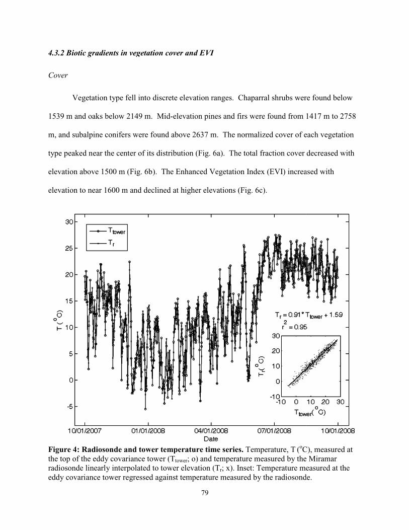
4.3.2 Biotic gradients in vegetation cover and EVI

Cover

Vegetation type fell into discrete elevation ranges. Chaparral shrubs

1539 m and oaks below 2149 m. Mid

m, and subalpine conifers were found

type peaked near the center of its distribution (Fig.

elevation above 1500 m (Fig. 6b). The Enhanced Vegetation Index (EVI) increa

elevation to near 1600 m and declined at higher elevations (Fig.

Figure 4: Radiosonde and tower temperature time series. the top of the eddy covariance tower (radiosonde linearly interpolated to tower elevation (eddy covariance tower regressed against temperature measured by the radiosonde.

79

nts in vegetation cover and EVI

tation type fell into discrete elevation ranges. Chaparral shrubs were found

m. Mid-elevation pines and firs were found from 1417

were found above 2637 m. The normalized cover of each vegetation

type peaked near the center of its distribution (Fig. 6a). The total fraction cover decreased with

b). The Enhanced Vegetation Index (EVI) increa

nd declined at higher elevations (Fig. 6c).

: Radiosonde and tower temperature time series. Temperature, T (oC),

the top of the eddy covariance tower (Ttower; o) and temperature measured by the Miramar interpolated to tower elevation (Tr; x). Inset: Temperature measured at the

eddy covariance tower regressed against temperature measured by the radiosonde.

were found below

from 1417 m to 2758

m. The normalized cover of each vegetation

a). The total fraction cover decreased with

b). The Enhanced Vegetation Index (EVI) increased with

C), measured at

; o) and temperature measured by the Miramar Temperature measured at the

eddy covariance tower regressed against temperature measured by the radiosonde.

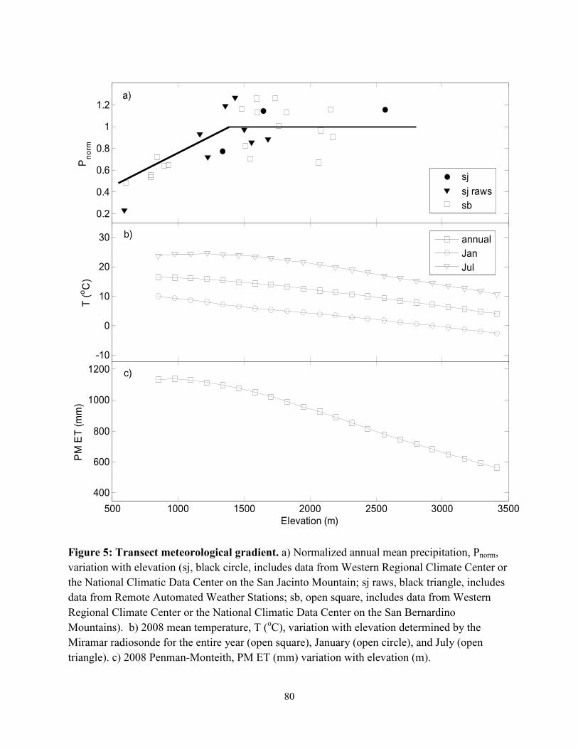
80

Figure 5: Transect meteorological gradient. a) Normalized annual mean precipitation, Pnorm, variation with elevation (sj, black circle, includes data from Western Regional Climate Center or the National Climatic Data Center on the San Jacinto Mountain; sj raws, black triangle, includes data from Remote Automated Weather Stations; sb, open square, includes data from Western Regional Climate Center or the National Climatic Data Center on the San Bernardino Mountains). b) 2008 mean temperature, T (oC), variation with elevation determined by the Miramar radiosonde for the entire year (open square), January (open circle), and July (open triangle). c) 2008 Penman-Monteith, PM ET (mm) variation with elevation (m).

0.2

0.4

0.6

0.8

1

1.2

Pno

rm

sjsj rawssb

-10

0

10

20

30

T (o C

)

annualJanJul

500 1000 1500 2000 2500 3000 3500

400

600

800

1000

1200

Elevation (m)

PM

ET

(mm

)

c)

b)

a)

81

Figure 6: Transect vegetation gradient. a) Normalized cover with elevation for selected Chaparral spp. (filled inverted triangle; Adenostoma fasciculatum, Arctostaphylos glandulosa, and Arctostaphylos glauca), Oak spp. (open circle; Quercus chrysolepis, kelloggii, and wislizenii), mid-elevation pines and firs (open star; mid-conifer; Abies concolor, Pinus coulteri, P. lambertiana, P. ponderosa, P. jeffreyi), and subalpine conifers (filled triangle; Pinus flexilis and P. contorta) b) Fraction Cover is the sum of all species cover divided by the length of the sampling transect (300 m) c) Enhanced Vegetation Index (EVI; filled inverted triangle; mean +/- 95% CI) variation with elevation. All plots show symbols at 122-m intervals connected by lines. Dashed vertical line indicates central site elevation.

0

0.5

1

1.5

Fra

ctio

n C

over

0

0.5

1

1.5N

orm

aliz

ed C

over

ChaparralOak

Mid ConiferSubalpine Conifer

500 1000 1500 2000 2500 3000 3500

0.15

0.2

0.25

0.3

0.35

EV

I

Elevation (m)

c)

b)

a)

Short-term controls on GEE at the central site

GEE increased rapidly with K

7). GEE was reduced at high and low temperatures (Fig.

ceased at -4oC. GEE was nearly consistent from 8

Figure 7: Light response curve. response to incoming solar radiation, K (W mdash; GEE(K)= 0.22 + ((18.36*K)/(K+565.79))) with the July through comparison, and b) July through August((22.10*K)/(K+624.44))) with the January through May regression for comparison (light dash).

82

rols on GEE at the central site

GEE increased rapidly with K under low light levels before saturating at

). GEE was reduced at high and low temperatures (Fig. 8). GEE declined below 8

GEE was nearly consistent from 8oC to 19oC and declined above 1

: Light response curve. Gross Ecosystem Exchange (GEE (µmol CO2 mresponse to incoming solar radiation, K (W m-2) for: a) January through May (2007 to 2009dash; GEE(K)= 0.22 + ((18.36*K)/(K+565.79))) with the July through August regression for

and b) July through August (2008 and 2009; bold solid; GEE(K)= 0.18 + with the January through May regression for comparison (light dash).

before saturating at higher K (Fig.

). GEE declined below 8oC and

C and declined above 19oC.

m-2 s-1)) 2007 to 2009; bold

August regression for bold solid; GEE(K)= 0.18 +

with the January through May regression for comparison (light dash).

83

Figure 8: Temperature scalar. Normalized Gross Ecosystem Exchange response to tower temperature, T0-1, for saturating incoming solar radiation (K > 500 W m-2) for January through May in (2007 to 2009; black triangle) and July through August ) 2008 and 2009; open triangle).

-10 0 10 20 30 400

0.2

0.4

0.6

0.8

1

1.2

1.4

T ( oC )

T0

-1

Jan-MayJul-Aug

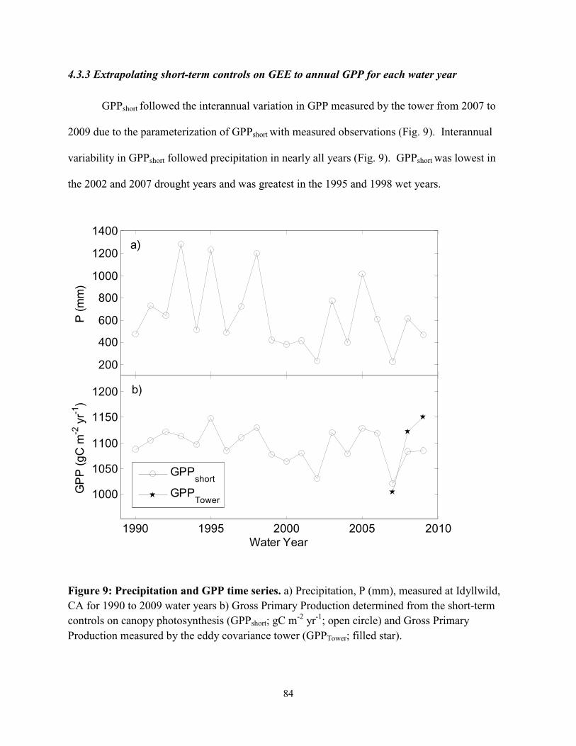
84

4.3.3 Extrapolating short-term controls on GEE to annual GPP for each water year

GPPshort followed the interannual variation in GPP measured by the tower from 2007 to

2009 due to the parameterization of GPPshort with measured observations (Fig. 9). Interannual

variability in GPPshort followed precipitation in nearly all years (Fig. 9). GPPshort was lowest in

the 2002 and 2007 drought years and was greatest in the 1995 and 1998 wet years.

Figure 9: Precipitation and GPP time series. a) Precipitation, P (mm), measured at Idyllwild, CA for 1990 to 2009 water years b) Gross Primary Production determined from the short-term controls on canopy photosynthesis (GPPshort; gC m-2 yr-1; open circle) and Gross Primary Production measured by the eddy covariance tower (GPPTower; filled star).

200

400

600

800

1000

1200

1400

P (m

m)

1990 1995 2000 2005 2010

1000

1050

1100

1150

1200

Water Year

GP

P (g

C m

-2 y

r-1)

GPPshort

GPPTower

b)

a)

85

4.3.4 Extrapolating the short-term controls on GEE at the central site to higher and lower

elevations

Seasonal summer reductions in precipitation forced vegetation to draw and deplete water

from the stored water pool, resulting in reductions in GEE. Complete reduction of the soil water

pool occurred at all elevations but occurred most often at low elevations. The fraction of

daytime observations with water limitation decreased with increasing elevation (Fig. 10), and the

fraction of daytime observations with temperature limitation increased with elevation.

Elevations between 1500 m and 2300 m had the greatest fraction of unstressed daytime

observations. GPPshort showed a smooth, broad pattern with elevation varying by less than 200

gC m-2 s-1 over the transect (Fig. 11). GPPshort was reduced by less than 20% at high elevations

due primarily to decreased temperatures, and at low elevations by decreased water availability

and increased temperatures (Fig. 10). GPPshort peaked near 2300 m, which was ~600 m above

the elevation of the central site and above the mixed pine and oak forest distribution that was

used to parameterize the GPPshort calculation (Fig. 11).

4.3.5 Long-term climate equilibrated GPP gradient

The elevational pattern of GPPlong was smooth over the transect with peak carbon uptake

at mid-elevations and reductions in carbon uptake at low and high elevations (Fig. 11). GPPlong

varied by two-fold across the transect, from 574 gC m-2 yr-1 to 1135 gC m-2 yr-1 around 1600 m.

86

Figure 10: Fraction of unstressed observation with elevation. Fraction of sunlight observation not limited by water (open inverted triangle), by temperature (open triangle), and by neither water nor temperature (black circle) for the 1990 – 2009 water years.

500 1000 1500 2000 2500 3000 3500

0.3

0.4

0.5

0.6

0.7

0.8

0.9

Elevation (m)

Fra

ctio

n of

uns

tress

ed s

unlig

ht o

bser

vatio

ns

WaterTemperatureWater and Temperature

87

Figure 11: GPPlong and GPPshort with elevation. Annual mean Gross Primary Production (GPP; gC m-2 yr-1; mean +/- 95% CI) for 2001 to 2009 water years determined by Enhanced Vegetation Index (GPPlong; filled triangle) and by GPPshort calculation (open circle). Vertical lines indicate the boundary between vegetation groups: Chaparral refers to Chaparral shrubs, Oak refers to Oak species, Mid conifer to Mid-elevation Pines and Firs, Subalpine refers to Subalpine conifers.

4.4 Discussion

4.4.1 Cover and GPP peaked at mid-elevation

Cover was greatest at mid-elevation. Fraction cover exceeded 100% at 1500 m from

overlapping tree canopies and declined with elevation above 1500 m (Fig. 6). Our survey went

500 1000 1500 2000 2500 3000 3500

500

600

700

800

900

1000

1100

1200

1300

GP

P (g

C m

-2 y

r-1)

Elevation (m)

GPPlong

GPPshort

Mid conifer SubalpineOakChaparral

88

as low as ~1295 m. Cover was likely similar or reduced at progressively lower elevations

through the Chaparral shrubland. The normalized cover of vegetation types rose and fell with

elevation (Fig. 5). Vegetation types shifted from small stature shrub and oak vegetation to larger

stature oak and conifer forests near 1500 m (Fig. 6). GPPlong was also greatest at mid-elevations

peaking near 1600 m (Fig. 11).

Previous studies have found similar elevational patterns of production, which correspond

to climate. Hanawalt and Whittaker [1976] indicated production peaked at mid-elevation in the

San Jacinto Mountains based on litter density. They attributed this pattern to precipitation and

temperature. Similar climate-related patterns were reported by Whittaker and Niering [1975] in

the Arizona’s Santa Catalina Mountains, where both precipitation and plant production increased

with elevation.

4.4.2 Can the short-term meteorological controls on canopy photosynthesis explain the long-

term relationship between climate and GPP?

The elevational patterns of temperature, precipitation, and PET were qualitatively

consistent with the hypothesis that meteorology controls the patterns of cover and productivity

(Fig. 5; Fig. 10). Drought limitation increased at lower elevations; cold limitation increased at

higher elevations; mid-elevations were comparatively less limited by either temperature or water,

leading to peak GPPshort at mid-elevation.

These controls, however, were insufficient to explain the magnitude of the long-term

pattern of GPP with elevation (Fig. 11). The discrepancies were large: GPPshort exceeded GPPlong

at high and low elevation; GPPshort varied less than 200 g m-2 yr-1 over the transect, whereas

89

GPPlong varied by over 550 g m-2 yr-1 (Fig. 11). These large discrepancies indicate that GPP was

shaped by more than the short-term controls on canopy gas exchange.

A discrepancy between short- and long-term responses of vegetation to meteorology has

been observed in experimental manipulations. For example, the short-term response in

community composition of tundra vegetation to light, temperature, and nutrient manipulations

was a poor predictor of the long-term response in community composition [Chapin et al., 1995].

The initial response of tundra vegetation to manipulations in meteorology were dominated by

growth whereas the long-term response reflected changes in growth, mortality, species

competition, and feedbacks to resource availability.

4.4.3 What might drive the discrepancy between GPPlong and GPPshort?

Leaf area is an important controller of GPP [Cowling and Field, 2003]. Accounting for

cover improved our prediction of the long-term pattern of GPP with elevation. In our initial

calculation, GPPshort was 91% to 140% of GPPlong from ~1500 to ~2500m. When we scaled

GPPshort by cover (GPPshort * cover at a given elevation / cover at central site elevation), the

scaled GPPshort values were 96% to 79% of GPPlong over the same elevation range. After

correcting for leaf area, GPPshort underestimated GPPlong , but the overall agreement in the

elevational pattern of GPP was improved: the underestimation was similar over a broad elevation

range and the pattern of GPP with elevation showed a similar decline to GPPlong.

While leaf area has a direct impact on GPP, additional climate controls and associated

feedbacks may also shape the elevational pattern of leaf area and GPP through their impacts on

90

species composition, stem density, or nutrient and water availability. We considered: 1)

feedbacks and thresholds to growth, 2) fire, and 3) soil properties.

Feedbacks and thresholds to growth

Small changes in meteorology may drive disproportionally large responses in GPP due to

positive feedbacks on ecosystem processes [Chapin et al., 1996]. Increased production in mid-

elevations may arise from feedbacks that reinforce and amplify the effect of a favorable

environment on productivity. Positive feedbacks to increased productivity may include the

development of taller vegetation, higher leaf area, and an extensive root system that subsequently

increase carbon uptake. For example, tall vegetation can support more leaves, and tall vegetation

may evade disturbances at the forest floor such as surface fires [Petit and Hampe, 2006]. Deeper

rooting and increased accesses to soil water may buffer vegetation from periodic droughts and

increase the growing season by avoiding summer drought [Arkley, 1981; Witty et al., 2003].

Thresholds in ecosystems may lead to sharp changes in vegetation and productivity with

small changes in the physical environment. For example, small changes in temperature or

climate extremes with elevation may lead to sharp change in meteorology (eg. freezing) that

drive shifts in vegetation. Additional thresholds may effect new sets of feedbacks that drive

shifts in vegetation distributions and productivity (eg. depth to stored water).

91

Fire

Fire is a key disturbance in Southern California’s montane ecosystems, resetting

succession and affecting species composition [Everett, 2008; Keeley and Davis, 2007; Minnich,

2007]. A shift in fire regime with elevation may be particularly important for setting species

composition that can affect carbon uptake. Fires in the low elevation Chaparral are often

characterized by high intensity crown fires [Keeley and Davis, 2007], whereas fires in higher

elevation conifer forests tend to be less intense ground fires [Everett, 2008]. Increased intensity

crown fires in low elevation shrubland favor the establishment of Chaparral species and

eliminate mixed conifer vegetation [Minnich, 2007]. This can effect a feedback in which the

establishment of Chaparral shrublands further promotes high intensity crown fires, which favor

the establishment of Chaparral shrublands. Chaparral shrublands tend to have lower productivity

than forests (eg. compare Sky Oaks with Blodgett Forest [Falge et al., 2002] or GPP at this

forest).

Soil constraints

Soil properties can control GPP by affecting nutrient and water availability [Chapin et

al., 2002]. We estimated water storage was 315 mm over the entire transect, an amount that is

consistent with water storage estimates in the top 3 to 3.5 m of regolith in Southern California

and the Sierra Nevada [Arkley, 1981; Witty et al., 2003]. However, soil properties almost

certainly change with elevation. Soil depth and clay content were greatest in mid-elevation on

the western slopes of the Southern Sierra Nevada Mountains, indicating locally increased

weathering [Dahlgren et al., 1997; O'Geen, 2007]. Deep soils at mid-elevation ranges may have

92

increased water storage capacity, potentially explaining the increased productivity in mid-

elevation forests.

4.4.4 Implications for the response of vegetation to climate change in montane California

We determined the response of vegetation to meteorology using a mid-elevation mixed

conifer forest. We extended this vegetation response to meteorology to the local montane

climate gradient and found that short-term constraints placed proportionally small limitations on

GPP at elevations where this forest type does not exist (Fig. 11).

In trying to understand how montane patterns of GPP will respond to climate change, an

approach that heavily weights short-term meteorological controls on production over additional

controls may not capture the actual response of vegetation to changes in climate. A mechanistic

understanding of long-term controls is required. Sorting out the relative importance of short- and

long-term controls has implications for the type, magnitude, and timescale of changes in GPP

with climate change. For example, thresholds and feedbacks in montane environments may lead

to punctuated responses of GPP to climate change. If meteorological controls on soil

development limit GPP, GPP may change much more slowly than changes in climate.

Key uncertainties remain: 1) landscape scale surveys of soil properties that directly

impact GPP, including total plant available water and 2) determination of a more mechanistic

understanding of the long-term controls on vegetation including identification and quantification

of thresholds and feedbacks in montane ecosystems. These uncertainties limit our understanding

of the response of vegetation to climate change.

93

Chapter 5: Has Fire Suppression Increased the

Amount of Carbon Stored in Western US Forests?

As appears in Fellows, A. W., and M. L. Goulden, Has fire suppression increased the amount of carbon stored in western U.S. forests?,Geophys. Res. Lett., 35, L12404, 2008.copyright 2008 American Geophysical Union. Reproduced/modified by permission of American Geophysical Union. 5.1 Abstract

Active 20th century fire suppression in western US forests, and a resulting increase in

stem density, is thought to account for a significant fraction of the North American carbon sink.

We compared California forest inventories from the 1930s with inventories from the 1990s to

quantify changes in aboveground biomass. Stem density in mid-montane conifer forests

increased by 34%, while live aboveground carbon stocks decreased by 26%. Increased stem

density reflected an increase in the number of small trees and a net loss of large trees. Large

trees contain a disproportionate amount of carbon, and the loss of large trees accounts for the

decline in biomass between surveys. 20th century fire suppression and increasing stand density

may have decreased, rather than increased, the amount of aboveground carbon in western US

forests.

94

5.2 Introduction

Active fire suppression since the early 20th century has caused a widespread increase in

the stem density of Western US forests [Chang, 1996]. The abundance of fire intolerant tree

species and smaller individuals has increased under a lengthened fire return interval, leading to

more dense forests [McKelvey et al., 1996]. Increased stand thickness has accelerated density

dependent and pest-induced mortality [Smith et al., 2005], and resulted in a shift from sparser

forests, which are dominated by a few large trees, to denser forests, which are dominated by

many small trees [Bouldin, 1999]. This trend is particularly pronounced in California’s mid-

elevation mixed conifer forest [Minnich et al., 1995].

The process of forest thickening is thought to result in the annual uptake of 2300 kg

C/ha/yr, which corresponds to an overall sink of 0.052 Pg Carbon/year for the western US

[Houghton et al., 1999], or 8 to 17% of the apparent 0.3 to 0.6 Pg C/yr conterminous US sink

[Goodale et al., 2002; Houghton and Hackler, 2000; Houghton et al., 1999; 2000; Pacala et al.,

2001]. However, the magnitude of the thickening-induced sink is highly uncertain, since it is

derived from only a few modeling [Covington and Moore, 1994; Hurtt et al., 2002; Keane et al.,

1990] and observational [Tilman et al., 2000] studies. A carbon sink associated with thickening

is intuitively appealing; increasing stem density must store more carbon in aboveground biomass

if all trees are equivalent. But the systematic loss of large trees, which contain a disproportionate

amount of carbon, requires a detailed consideration of the associated demographic shifts.

We compared forest inventory observations from the 1930s that were made in California

by the Weislander Vegetation Type Mapping project (VTM; [Minnich et al., 1995; Weislander,

95

1935]) with observations from the 1990s made by the Forest Inventory Analysis (FIA; [Waddell

et al., 2005]). Our goals were to characterize the demographic shifts in California forest over the

60-year period and to quantify the change in carbon stored in aboveground live biomass with

thickening.

5.3 Methods

269 VTM plots were compared with 260 FIA plots from spatially overlapping, legally

designated wilderness areas in California to determine how stem density and aboveground

biomass changed from the 1930s to 1990s. We obtained VTM data from the Weislander

Vegetation Type Mapping Project at the University of California, Berkeley (vtm.berkeley.edu)

and FIA data from the United States Forest Service (http://fia.fs.fed.us/).

The plots measured during the two surveys were not collocated, and, in many cases, it has

proven difficult to identify the precise location of the original VTM plots [Keeley, 2004]. We

therefore compared large samples of plots from the two studies. Designated wilderness is

generally inaccessible and not logged, which reduces the likelihood of confounding changes in

forest structure caused by active management. The selected plots spanned much of California,

and covered large ranges of elevation, mean annual precipitation (MAP), forest type, and fire

regime.

The VTM recorded the number of trees by species in four size classes within 0.08 ha

plots during 1929 to 1934 (10-30 cm, 30-61cm, 61-91 cm, and >91cm). The FIA recorded tree

diameter by species within multiple fixed and variable radius plots during 1990 to 1994. We

homogenized the methods by correcting the area of the VTM plots for topography to match the

96

FIA methods, using the recorded slope and simple trigonometric functions. Differences in plot

selection criteria between the VTM and FIA required us to omit plots with no trees from the

analysis [Bouldin, 1999]. We degraded the FIA DBH information by binning individuals into

VTM size classes.

The estimation of biomass from stem counts requires information on the average biomass

for each species and size bin. The VTM resolution does not allow us to accurately determine the

biomass for each bin. We therefore used the average biomass determined from the FIA data and

applied it to both the VTM and FIA species and size bins. The average biomass for each bin

was determined by extrapolating the DBH of each reserved tree in the FIA to aboveground

biomass using aggregated allometric equations and then averaging over the species and size bin

[Jenkins et al., 2003]. Reserved trees are in forests that are closed to harvest, which included

plots both inside and outside of our analysis areas. For groupings with < 30 trees, average

biomass was determined from both reserved and non-reserved forests or, in limited cases, from a

congener with similar biomass characteristics. Giant Sequoia, Sequoiadendron giganteum,

average biomass was determined from reserved areas despite having fewer than 30 trees because

this value was within the range of other species. We converted biomass to carbon using 0.45 g

C/g biomass.

Historical accounts indicate that early 1900’s forests contained larger trees than

contemporary forests [Bouldin, 1999]. Our reliance on the FIA dataset to determine the average

biomass for each bin provides a conservative estimate of VTM biomass. Aggregated allometric

equations often reduce the errors associated with variations in geographic range, species

composition, and size distribution, but may lead to errors of as much as 30%, when compared to

site-specific allometric equations [Jenkins et al., 2003]. These types of error may have impacted

97

the accuracy of our biomass estimates, but would not be expected to affect the comparison

between data sets.

Changes in stem density and carbon content between the surveys were compared as a

function of elevation, precipitation, forest type, and geographic location. The forest type for each

plot was identified using the GAP LANDCOV spatial dataset [Davis et al., 1998]. Plot elevation

and MAP were determined using spatial data sets from the California Spatial Library [CaSIL,

2000; Teale, 1997].

Data were square root transformed and tested for normality using a Kolmogorov-Smirnov

test. All data were normally or near normally distributed after transformation. A two-sample t-

test assuming unequal variance was used to determine statistical difference. Reported means are

back transformed means of the square root transformed data.

5.4 Results

The stem density averaged across all plots increased by an insignificant 4% from the

1930s to the 1990s (Tab. 1). By contrast, the live aboveground carbon stocks declined by a

highly significant 34%, which corresponds to an average loss of ~0.7 Mg C/ha/year between

surveys (Tab. 1; p <0.001).

98

Stand Density (stems ha-1) Carbon in Biomass (Mg ha-1) Count Category VTM FIA % p VTM FIA % p n(VTM) n (FIA)

Elevation (m): 0-914: 281 181 -36 0.05 97 73 -25 0.26 39 26

914-2438: 204 242 19 0.10 126 77 -39 <0.001 151 180 >2438: 231 233 1 0.96 123 89 -28 0.04 79 54

All: 223 233 4 0.54 120 79 -34 <0.001 269 260 Forest Type:

mid-montane conifer: 195 261 34 0.07 118 87 -26 0.10 53 77

upper-montane conifer: 240 254 6 0.72 172 122 -29 0.03 76 44

Precipitation in conifer (cm)

1-114: 226 194 -14 0.45 97 68 -30 0.14 35 46 ≥114: 219 302 38 0.013 171 121 -29 0.01 94 75

Geographic Region:

NorCa/Sierra: 206 269 31 0.008 138 100 -28 0.004 154 140 SoCa/Tr/Vent: 245 195 -20 0.06 99 53 -46 <0.001 115 120

Table 1: Stand density and carbon stored in aboveground live biomass for various categories. VTM gives mean values for 1929-1934 forests for the region studied. FIA gives mean values for the 1990-1994 forests for the region studied. p gives p-value for significance of change between VTM and FIA surveys. Mid-montane conifer forests include Sierra mixed conifer, ponderosa pine, Jeffrey pine, white fir, and mixed conifer-hardwood forests in the GAP dataset. Upper-montane forests include subalpine conifer and red fir forests in the GAP dataset. Precipitation in conifer (cm) includes plots from both upper and mid-montane conifer plots for mean annual precipitation amounts <114 cm and ≥114 cm. NorCa/Sierra are plots in northern California or the Sierra Nevada Range. SoCa/Tr/Vent are plots in Southern California, Transverse Range, or Ventana wilderness.

The changes in density and biomass varied with forest type (Tab. 1). Middle elevation

plots (914 to 2438m) showed the greatest increases in stem density and decreases in

aboveground biomass. Higher elevation plots had a constant stem density and a more modest

decline in biomass. Lower elevation plots showed declines in both stem density and biomass.

Changes in structure also depended on precipitation. Conifer plots receiving a MAP of at least

114 cm thickened (p=0.01), whereas plots receiving a MAP of less than 114 cm showed no

99

change in stem density. Geographical regions exhibited contrasting trends. Plots pooled from

Northern California and the Sierra Nevada Mountains showed a significant increase in stem

density and a significant loss of carbon, whereas plots pooled from Southern California, the

Ventana wilderness, and Transverse range showed an insignificant thinning and a highly

significant loss of carbon.

The trend towards increasing tree density and decreasing biomass was especially

pronounced within wet (>= 114 cm MAP) conifer (Ponderosa Pine, Jeffrey Pine, Sierra Mixed

conifer, White Fir, Mixed Hardwood Conifer forests, Subalpine conifer, and Red Fir) forests

(Tab. 1; Figure 1). The stem density in these forests increased by 38%, while the aboveground

biomass decreased by 29%. The size structure of these forests changed markedly over time. The

increase in stem density was driven entirely by smaller trees. Increases in 10-30 cm DBH trees

(p<0.001) and 30-61 cm DBH trees (p=0.02) led to an increase of 119 stems/ha and a gain of ~17

MgC/ha in aboveground biomass. At the same time, declines in 61-90 cm DBH trees (p=0.001)

and >90 cm DBH trees (p=0.007) led to a decrease of 29 stems/ha and a loss of 64 MgC/ha. The

loss of carbon from large trees outweighed the gain in small trees, resulting in an overall loss of

carbon in aboveground biomass.

100

a )

Ste

m d

ensi

ty (

stem

s ha

-1)

0

1 0 0

2 0 0

3 0 0

4 0 0

V T M (~ 1 9 3 0 )F IA (~ 1 9 9 0 )

b )

D B H s iz e c la s s (c m )

to ta l 1 0 -3 0 3 0 -6 1 6 1 -9 1 > 9 1

Car

bon

in li

ve a

bove

grou

nd

biom

ass

(MgC

ha-

1)

0

5 0

1 0 0

1 5 0

2 0 0

2 5 02 5 0

Figure 1: Tree density and carbon storage by tree size. Median and 95% confidence intervals for (a) tree density and (b) carbon stored in live aboveground biomass for conifer forests receiving ≥ 114cm mean annual precipitation.

5.5 Discussion

5.5.1 Patterns of forest density and biomass

The increases in stand density we observed are consistent with the patterns of forest

thickening that have been reported in previous studies. We observed the greatest increases in

stem density in mid-elevation conifer forests, where fire suppression is believed to have altered

101

historic fire regimes the most. Previous studies have also reported that thickening has been

greatest at mid elevation (cf. [Bouldin, 1999; Minnich et al., 1995]). Higher elevation forests

showed a negligible amount of thickening (Tab. 1), a pattern that is generally attributed to a

longer natural fire return interval and a reduced impact of fire suppression [Chang, 1996].

Previous studies have shown that the increase in stem density is driven almost entirely by an

increase in the smaller classes, and that the abundance of larger trees has decreased (cf. [Bouldin,

1999; Minnich et al., 1995]). Bouldin [1999] and Minnich et al. [1995] reported somewhat

greater rates of stand density increases than we found. This discrepancy may arise from our

focus on wilderness. Some of the plots analyzed by Bouldin [1999] may have been logged,

which would be expected to result in a greater increased density of small trees.

We observed thinning in low elevation forests (p=0.05). This thinning was driven by a

reduction in smaller (<61 cm) trees (p=0.07) and the retention of larger trees. These patterns

may indicate a lack of recruitment in low elevation forests. Several reports indicate that

regeneration of California oaks is currently poor, especially at low elevations, on sites with a

southern aspect or thin soil, and in areas that have a low MAP [Standiford et al., 1996].

Fire suppression leads to an accumulation of carbon in Coarse Woody Debris (CWD) and

the forest floor [McKelvey et al., 1996]. Using expansion factors embedded in the FIA database

indicates that California’s reserved forests contain 17±0.9 Mg C/ha (standard error) of CWD and

standing dead trees. This is less than the 41 Mg C/ha lost from aboveground biomass implying

that much of the carbon lost from aboveground biomass has already decayed.

Previous analyses indicate that California’s forests sequestered carbon during 1990 to

2002 and that this uptake was greatest where past management caused forest regrowth [Bemis

102

and Allen, 2005]. Our findings neither confirm nor contradict these results. We focused on

wilderness areas, where active management did not occur. Moreover, Bemis and Allen [2005]

examined forest changes over 12 years during the 1990s, whereas we integrated changes in

Californian forest from the 1930s to 1990s.

5.5.2 Mechanism accounting for biomass loss with thickening

The forest thickening we observed did not result in a large increase in aboveground

biomass, as has been assumed [Houghton et al., 1999]. The relationship between DBH and

biomass is markedly non-linear [Jenkins et al., 2003]. A single large tree (>90 cm) contains the

same amount of carbon as 60 small (10-30 cm) trees. Trees <61 cm DBH accounted for nearly

85% of the total stems across all surveys, but just ~33% of the biomass. We found that

thickening was largely driven by an increase in small trees, which stored a small amount of

carbon. Thickened forests also showed a reduction in the number of large trees, which stored a

large amount of carbon. The loss of carbon from the reduction in large trees outweighed the gain

in carbon from the increase in small trees and resulted in an overall loss of aboveground

biomass.

Trees in denser forests face greater competition for water and other resources. Ponderosa

pines in high-density stands have lower xylem water potentials and rates of photosynthesis,

indicating greater drought stress [Kolb et al., 1998]. These trees also have decreased resin

production and foliar toughness, suggesting an increased susceptibility to insect and pathogen

attack [Kolb et al., 1998]. Western conifer forests undergo periodic drought associated with

climatic cycles such as the Pacific Decadal Oscillation [Swetnam and Betancourt, 1998]. Trees

103

that are growing in denser stands are thought to be especially vulnerable to attack or mortality

during dry periods [Kolb et al., 1998; Smith et al., 2005].

Large trees may be particularly prone to mortality under these conditions [Smith et al.,

2005]. Some bark beetles prefer large trees, which have a thicker phloem ([Cole et al., 1969];

but see [Kolb et al., 2006]). Large trees may have increased vulnerability to cavitation during

drought, either because their leaves are higher off the ground or because restrictions in the xylem

cause more negative xylem water potential compared with small trees [Hubbard et al., 1999].

Large trees may be more exposed to wind and radiation than small trees, further increasing

drought stress. Large trees may have higher respiration costs associated with greater biomass

([Makela and Valentine, 2001]; but see [Ryan and Waring, 1992]). Finally, large trees are often

approaching the end of their natural lifespan [Day et al., 2001].

The effect of thickening on stand structure in California’s conifer forests appears simple,

direct, and strong. Fire suppression increases the density, and, probably, the leaf area, of forest.

The trees in denser forests are exposed to greater stress during periodic extreme drought. Large

trees are more likely to suffer mortality than small trees. Fire suppression leads over time to a

forest with more small trees and fewer large trees. Large trees contain a disproportionate amount

of biomass. Fire suppression in California’s conifer forests therefore leads to an increase in stand

density and a decrease in aboveground biomass due to a loss of large trees. This loss of carbon

from aboveground biomass in thickened stands conflicts with the assumption that forest

thickening in western forests has led to a significant carbon sink in North America, and

underscores the importance of demography as a controller of forest carbon balance.

104

Chapter 6: Conclusion

6.1 Overview

Chapters two through four of this dissertation focused on how weather affects vegetation

in California’s Mountains. Chapter 2 addressed how tree mortality associated with drought

impacted vegetation distributions. Chapter 3 addressed how climate controls the productivity of

a low elevation forest and explored how a semi-arid low elevation forest survives at the warm

and dry edge of its range. Chapter 4 asked whether short-term controls on vegetation

productivity alone can explain the overall pattern in productivity with elevation, and concluded

that additional climate equilibrated controls help shape the overall pattern of productivity with

elevation. Chapter 5 addressed how fire suppression may affect carbon storage in California’s

forests.

6.1.1 Brief chapter review

Chapter 2

We examined the pattern of widespread tree mortality that occurred in 2002-04 in the San

Jacinto Mountains. Conifer mortality was likely triggered by drought and was focused in low

elevation mid-montane forests. Tree mortality in the low elevation range led to a rapid

105

redistribution of vegetation characterized by an upslope shift in the cover-weighted mean

elevation of mid-montane conifer trees. Drought driven tree mortality has occurred during past

dry periods, indicating that drought driven forest mortality may be cyclical and that past species’

distribution shifts may have occurred with past changes in meteorology.

Chapter 3

We investigated forest function in a mixed conifer forest near its warm and dry ecotone.

Low temperatures placed weak controls on forest Gross Primary Productivity (GPP). High vapor

pressure deficit placed proportionally greater control on GPP. Reductions in precipitation

appeared to drive large reductions in GPP, which was most evident in the late 2007 and early

2008 water years. This forest survived at its low elevation ecotone by maintaining high carbon

uptake at low temperatures and extracting water stored in deep soils, which extended its growing

season.

Chapter 4

We considered the effect of direct short-term meteorological controls on canopy-level

photosynthesis in shaping the long-term pattern in GPP with elevation. Short-term constraints on

GPP were driven by reduced temperatures at high elevations and by increased temperatures and

reduced water availability at low elevations leading to a comparatively longer growing season in

the mid-elevation range. Short-term controls, however, were insufficient to explain the

magnitude of change in GPP with elevation indicating that additional controls are required to

reconcile the discrepancy.

106

Chapter 5

Active 20th century fire suppression in western US forests and a resulting increase in stem

density are thought to account for a significant fraction of the North American carbon sink. We

compared the 1930s Vegetation Type Mapping dataset with the 1990s Forest Inventory Analysis

dataset to quantify changes in aboveground biomass. We found a change in forest structure

characterized by an increase in stem density and a net loss of large trees. Large trees contain a

disproportionate amount of carbon, and a loss of large trees accounts for the decline in biomass

between surveys. 20th century fire suppression and increasing stand density do not appear to lead

to a large increase in carbon stored in aboveground biomass.

6.2 General Conclusions

Climate change is anticipated to have large impacts on the biosphere and appears to have

already led to shifts in the phenology, species distributions, community composition, and

changes in the structure and function of ecosystems ( for reviews: [McCarty, 2001; Parmesan,

2006; Parmesan and Yohe, 2003; Walther et al., 2002]). Outstanding questions remain: Will

vegetation respond rapidly or slowly? Will vegetation redistribute under climate change? What

are the ecosystem properties and climate factors that lead to sensitivity of vegetation to

meteorology?

This dissertation addresses these questions by investigating climate-mediated tree

mortality and the response of a low elevation mixed conifer forest to meteorology in California’s

mountains. Observed tree mortality in 2002-04 in the semi-arid San Jacinto Mountains was

107

widespread, rapid, and focused at low elevations. The patterns of conifer mortality were

consistent with reduced precipitation associated with climate variability. Past drought associated

with climate variability may have driven similar patterns in tree mortality and associated species

redistribution over the history of this forest. Similarly, future shifts in climate and possible

reductions in precipitation may lead to rapid vegetation redistribution through similar drought

driven tree mortality and an upslope “lean” in vegetation distributions.

In principle, low elevation forests located at their warm and dry range margin are at

greatest risk to climate change. The sensitivity of low elevation forests to climate change

depends on the function of these forests. Mixed conifer forests maintain a year-round carbon

uptake by using water stored in deep water pools and maintaining high rates of carbon uptake at

low temperatures. These attributes allow mixed conifer forests to persist despite a long seasonal

drought and high evaporative demand during summer periods. However, this function may also

make these forests vulnerable to climate change.

The predicted increase in temperature with climate change would have a minimal direct

effect on winter carbon uptake in low elevation forests. However, concomitant increases in

summer vapor pressure deficit (VPD) are anticipated to drive a relatively large reduction in GPP.

Decreased precipitation appears to drive large reductions in GPP under severe drought years and

may have a threshold beyond which forests begin to show signs of stress. Increased VPD and

reduced water availability could have large impacts on low elevation vegetation under climate

change. This finding, combined with the observed patterns of drought-driven conifer mortality

provides evidence that semi-arid forests at their warm and dry range margins will be susceptible

to climate change.

108

However, the response of montane forests to climate change will require understanding

how soil water availability varies at the landscape scale and will require understanding additional

long-term controls on productivity, including feedbacks and thresholds that may have non-linear

effects on vegetation and productivity. A mechanistic understanding of these long-term controls

will be needed to predict how vegetation will respond to climate change.

6.3 Things to have done differently

Identification of the elevational pattern in tree mortality would have been strengthened by

including similar surveys on additional slopes or additional mountain ranges in Southern

California. A stronger approach may have repeated surveys of previous vegetation inventories.

Hamilton [1983] and Wright [1966], for example, report data from Southern California

mountains that might be available for determining how vegetation changed with elevation.

The response of individual species to weather would have been improved by including

measurements at the individual tree scale. For example, the use of sap flow sensors would have

established a continuous time series of vegetation processes at the species level. Coupling these

measurements with targeted leaf gas exchange measurements (spot measurements, response

curves, etc.) may have provided additional information about climate controls on species

function at the individual level.

More generally, closing the water budget along the elevation gradient may have given us

more information about how vegetation responds to climate. In particular, we need to understand

weather, soil depth, and soil water holding capacity over the broad landscape.

109

6.4 Future Work

Some questions:

Was tree mortality greatest at the lower portion of a species’ range over the broader landscape?

Kelly and Goulden [2008] indicated that tree mortality was also greatest at the low elevation

species’ range limit. However, incorporating additional mountain ranges and a broader

geographical range would strengthen these observations.

These forests appeared to have undergone past periods of high tree mortality coincident with past

drought associated with climate variability, and this may have led to previous vegetation

distribution shifts. However, we still don’t know how stable vegetation distributions are with

respect to changes in weather/climate at different timescales. How much must climate change to

see long-term shifts in vegetation distributions? This will require an improved understanding of

the different controls on processes and feedbacks that shape vegetation distributions.

What are the impacts of tree mortality on the landscape? How do biogeochemistry, hydrology,

and vegetation recover from tree mortality? Similarly high periods of tree mortality have

occurred in the past. A chronosequence of the time since tree mortality may be a useful

experimental design.

110

References

Abatzoglou, J. T., K. T. Redmond, and L. M. Edwards (2009), Classification of Regional Climate Variability

in the State of California, Journal of Applied Meteorology and Climatology, 48(8), 1527-1541.

Adams, H. D., M. Guardiola-Claramonte, G. A. Barron-Gafford, J. C. Villegas, D. D. Breshears, C. B. Zou, P.

A. Troch, and T. E. Huxman (2009), Temperature sensitivity of drought-induced tree mortality portends

increased regional die-off under global-change-type drought, Proceedings of the National Academy of

Sciences, 106(17), 7063-7066.

Adams, H. D., A. K. Macalady, D. D. Breshears, C. D. Allen, N. L. Stephenson, S. R. Saleska, T. E. Huxman,

and N. g. McDowell (2010), Climate-Induced Tree Mortality: Earth System Consequences, Eos Trans.

AGU, 91(17).

Allen, C. D., and D. D. Breshears (1998), Drought-induced shift of a forest–woodland ecotone: Rapid

landscape response to climate variation, Proceedings of the National Academy of Sciences, 95(25),

14839-14842.

Allen, C. D., et al. (2010), A global overview of drought and heat-induced tree mortality reveals emerging

climate change risks for forests, in Forest Ecology and Management, edited, pp. 660-684.

Anderson, R. G., and M. L. Goulden (2011), Relationships between climate, vegetation, and energy

exchange across a montane gradient, J. Geophys. Res., 116(G1), G01026.

Ansley, J.-A. S., and J. J. Battles (1998), Forest Composition, Structure, and Change in an Old-Growth

Mixed Conifer Forest in the Northern Sierra Nevada, Journal of the Torrey Botanical Society, 125(4), 297-

308.

Arkley, R. J. (1981), Soil Moisture Use by Mixed Conifer Foret in a Summer-Dry Climate, Soil Science

Society of America(45), 423-427.

Armstrong, C. F., and C. K. Stidd (1967), A moisture-balance profile on the Sierra Nevada, Journal of

Hydrology(5), 258-268.

Beckage, B., B. Osborne, D. G. Gavin, C. Pucko, T. Siccama, and T. Perkins (2008), A rapid upward shift of

a forest ecotone during 40 years of warming in the Green Mountains of Vermont, Proceedings of the

National Academy of Sciences, 105(11), 4197-4202.

Bemis, G. R., and J. Allen (2005), Inventory of California greenhouse gas emissions and sinks: 1990-2002

update, in Report CEC-600-2005-025, edited, California Energy Commission, Sacramento, Calif.

Biondi, F., Alexander Gershunov, Daniel R. Cayan (2001), North pacific decadal climate variability since

1661, Journal of Climate(14), 5-10.

Bouldin, J. (1999), Twentieth-century changes in forests of the Sierra Nevada, California, Ph.D. thesis, UC

Davis.

111

Breshears, D. D., T. E. Huxman, H. D. Adams, C. B. Zou, and J. E. Davison (2008), Vegetation

synchronously leans upslope as climate warms, Proceedings of the National Academy of Sciences,

105(33), 11591-11592.

Breshears, D. D., et al. (2005), Regional vegetation die-off in response to global-change-type drought,

Proceedings of the National Academy of Sciences of the United States of America, 102(42), 15144-15148.

Campbell, G. S., and J. M. Norman (1998), An Introduction to Environmental Biophysics, 2 ed., Springer-

Verlag New York.

CaSIL (2000), Digital Elevation Maps (DEM), edited, California Spatial Information Library, Sacramento,

CA.

Cayan, D., K. T. Redmond, and L. G. Riddle (1999), ENSO and Hydrologic Extremes in the Western United

States*, Journal of Climate, 12(9), 2881-2893.

Cayan, D., E. Maurer, M. Dettinger, M. Tyree, and K. Hayhoe (2008), Climate change scenarios for the

California region, Climatic Change, 87(0), 21-42.

Chang, C.-R. (1996), Ecosystem responses to fire and variations in fire regimes, in Sierra Nevada

Ecosystem Project: Final Report to Congress, 2, 1041-1069, edited, University of California, Center for

Water and Wildland Resources, Davis, CA.

Chapin, F. S., M. S. Torn, and M. Tateno (1996), Principles of Ecosystem Sustainability, The American

Naturalist, 148(6), 1016-1037.

Chapin, F. S., P. A. Matson, and H. A. Mooney (2002), Principles of Terrestrial Ecosystem Ecology, 472

pp., Springer-Verlag, New York.

Chapin, F. S., G. R. Shaver, A. E. Giblin, K. J. Nadelhoffer, and J. A. Laundre (1995), Responses of Arctic

Tundra to Experimental and Observed Changes in Climate, Ecology, 76(3), 694-711.

Cole, W. E., G. D. Amman, and Intermountain Forest and Range Experiment Station (Ogden Utah) (1969),

Mountain pine beetle infestations in relation to lodgepole pine diameters, 7 p. pp., U.S. Dept. of

Agriculture Forest Service Intermountain Forest & Range Experiment Station, Ogden, Utah.

Covington, W. W., and M. M. Moore (1994), Southwestern Ponderosa Forest Structure - Changes since

Euro-American Settlement, J Forest, 92(1), 39-47.

Cowling, S. A., and C. B. Field (2003), Environmental control of leaf area production: Implications for

vegetation and land-surface modeling, Global Biogeochem. Cycles, 17(1), 1007.

Crimmins, S. M., S. Z. Dobrowski, J. A. Greenberg, J. T. Abatzoglou, and A. R. Mynsberge (2011), Changes

in Climatic Water Balance Drive Downhill Shifts in Plant Species’ Optimum Elevations, Science,

331(6015), 324-327.

Dahlgren, R. A., J. L. Boettinger, G. L. Huntington, and R. G. Amundson (1997), Soil development along an

elevational transect in the western Sierra Nevada, California, Geoderma, 78(3-4), 207-236.

Day, M. E., M. S. Greenwood, and A. S. White (2001), Age-related changes in foliar morphology and

physiology in red spruce and their influence on declining photosynthetic rates and productivity with tree

age, Tree Physiology, 21(16), 1195-1204.

112

Everett, R. G. (2008), Dendrochronology-based fire history of mixed-conifer forests in the San Jacinto

Mountains, California, Forest Ecology and Management, 256(11), 1805-1814.

Falge, E., et al. (2002), Seasonality of ecosystem respiration and gross primary production as derived

from FLUXNET measurements, Agricultural and Forest Meteorology, 113(1-4), 53-74.

Flint, A. L., G. S. Campbell, K. M. Ellett, and C. Calissendorff (2002), Calibration and Temperature

Correction of Heat Dissipation Matric Potential Sensors, Soil Sci. Soc. Am. J., 66(5), 1439-1445.

Franklin, J. F., H. H. Shugart, and M. E. Harmon (1987), Tree Death as an Ecological Process, BioScience,

37(8), 550-556.

Goodale, C. L., et al. (2002), Forest carbon sinks in the Northern Hemisphere, Ecol Appl, 12(3), 891-899.

Goulden, M. L., G. C. Winston, A. M. S. McMillan, M. E. Litvak, E. L. Read, A. V. Rocha, and J. Rob Elliot

(2006), An eddy covariance mesonet to measure the effect of forest age on land–atmosphere exchange,

Global Change Biology, 12(11), 2146-2162.

Grulke, N. E., W. Dobrowolski, P. Mingus, and M. E. Fenn (2005), California black oak response to

nitrogen amendment at a high O3, nitrogen-saturated site, Environmental Pollution, 137(3), 536-545.

Hamilton, M. P. (1983), A Floristic Basis for the Management of Rare Plants and Their Communities in

the San Jacinto Mountains, California, Cornell University.

Hanawalt, R. B., and R. H. Whittaker (1976), Altitudinally Coordinated Patterns of Soils and Vegetation

in-the San Jacinto Mountains, California, Soil Science, 121(2), 114-124.

Hayhoe, K., et al. (2004), Emissions pathways, climate change, and impacts on California, Proceedings of

the National Academy of Sciences of the United States of America, 101(34), 12422-12427.

Helliker, B. R., and S. L. Richter (2008), Subtropical to boreal convergence of tree-leaf temperatures,

Nature, 454(7203), 511-514.

Houghton, R. A., and J. L. Hackler (2000), Changes in terrestrial carbon storage in the United States. 1:

The roles of agriculture and forestry, Global Ecol Biogeogr, 9(2), 125-144.

Houghton, R. A., J. L. Hackler, and K. T. Lawrence (1999), The US carbon budget: Contributions from

land-use change, Science, 285(5427), 574-578.

Houghton, R. A., J. L. Hackler, and K. T. Lawrence (2000), Changes in terrestrial carbon storage in the

United States. 2: The role of fire and fire management, Global Ecol Biogeogr, 9(2), 145-170.

Hubbard, R. M., B. J. Bond, and M. G. Ryan (1999), Evidence that hydraulic conductance limits

photosynthesis in old Pinus ponderosa trees, Tree Physiology, 19(3), 165-172.

Huete, A., K. Didan, T. Miura, E. P. Rodriguez, X. Gao, and L. G. Ferreira (2002), Overview of the

radiometric and biophysical performance of the MODIS vegetation indices, Remote Sensing of

Environment, 83(1-2), 195-213.

Hurtt, G. C., S. W. Pacala, P. R. Moorcroft, J. Caspersen, E. Shevliakova, R. A. Houghton, and B. Moore

(2002), Projecting the future of the US carbon sink, Proceedings of the National Academy of Sciences of

the United States of America, 99(3), 1389-1394.

113

Jenkins, J. C., D. C. Chojnacky, L. S. Heath, and R. A. Birdsey (2003), National-scale biomass estimators for

United States tree species, Forest Science, 49(1), 12-35.

Jin, Y., J. T. Randerson, and M. L. Goulden (2011), Continental-scale net radiation and evapotranspiration

estimated using MODIS satellite observations, Remote Sensing of Environment, 115(9), 2302-2319.

Jump, A. S., C. Mátyás, and J. Peñuelas (2009), The altitude-for-latitude disparity in the range retractions

of woody species, Trends in Ecology & Evolution, 24(12), 694-701.

Keane, R. E., S. F. Arno, and J. K. Brown (1990), Simulating Cumulative Fire Effects in Ponderosa Pine

Douglas-Fir Forests, Ecology, 71(1), 189-203.

Keeley, J. E. (2004), VTM Plots as Evidence of Historical Change: Goldmine or Landmine?, Madrono, 51,

372-378.

Keeley, J. E., and F. W. Davis (2007), Chaparral, in Terrestrial Vegetation of California, edited by M. G.

Barbour, Todd Keeler-Wolf, Allan A. Schoenherr, pp. 339-366, University of California Press, Berkeley

and Los Angeles.

Kelly, A. E., and M. L. Goulden (2008), Rapid shifts in plant distribution with recent climate change,

Proceedings of the National Academy of Sciences, 105(33), 11823-11826.

Kolb, T. E., and J. E. Stone (2000), Differences in leaf gas exchange and water relations among species

and tree sizes in an Arizona pine–oak forest, Tree Physiology, 20(1), 1-12.

Kolb, T. E., K. M. Holmberg, M. R. Wagner, and J. E. Stone (1998), Regulation of ponderosa pine foliar

physiology and insect resistance mechanisms by basal area treatments, Tree Physiology, 18(6), 375-381.

Kolb, T. E., N. Guerard, R. W. Hofstetter, and M. R. Wagner (2006), Attack preference of Ips pini on Pinus

ponderosa in northern Arizona: tree size and bole position, Agr Forest Entomol, 8(4), 295-303.

Kurz, W. A., C. C. Dymond, G. Stinson, G. J. Rampley, E. T. Neilson, A. L. Carroll, T. Ebata, and L. Safranyik

(2008), Mountain pine beetle and forest carbon feedback to climate change, Nature, 452(7190), 987-

990.

Law, B. E., et al. (2002), Environmental controls over carbon dioxide and water vapor exchange of

terrestrial vegetation, Agricultural and Forest Meteorology, 113(1-4), 97-120.

Lenoir, J., J. C. Gégout, P. A. Marquet, P. de Ruffray, and H. Brisse (2008), A Significant Upward Shift in

Plant Species Optimum Elevation During the 20th Century, Science, 320(5884), 1768-1771.

Loarie, S. R., B. E. Carter, K. Hayhoe, S. McMahon, R. Moe, C. A. Knight, and D. D. Ackerly (2008), Climate

Change and the Future of California's Endemic Flora, PLoS ONE, 3(6), e2502.

Lundquist, J. D., and S. P. Loheide, II (2011), How evaporative water losses vary between wet and dry

water years as a function of elevation in the Sierra Nevada, California, and critical factors for modeling,

Water Resour. Res., 47, W00H09.

Makela, A., and H. T. Valentine (2001), The ratio of NPP to GPP: evidence of change over the course of

stand development, Tree Physiology, 21(14), 1015-1030.

114

McCabe, G. J., M. A. Palecki, and J. L. Betancourt (2004), Pacific and Atlantic Ocean influences on

multidecadal drought frequency in the United States, Proceedings of the National Academy of Sciences,

101(12), 4136-4141.

McCarty, J. P. (2001), Review: Ecological Consequences of Recent Climate Change, Conservation Biology,

15(2), 320-331.

McDowell, N., et al. (2008), Mechanisms of plant survival and mortality during drought: why do some

plants survive while others succumb to drought?, New Phytologist, 178(4), 719-739.

McKelvey, K., C. Skinner, C.-R. Chang, D. Erman, S. Husari, D. Parsons, J. Wagtendonk, and C.

Weatherspoon (1996), An overview of fire in the Sierra Nevada, 2, in Sierra Nevada Ecosystem Project:

Final Report to Congress, edited, pp. 1033-1039, University of California, Center for Water and Wildland

resources, Davis, CA.

Millar, C. I., Robert D. Westfall, Diane L. Delany, John C. King and Lisa J. Graumlich (2004), Response of

Subalpine Conifers in the Sierra Nevada, California, U.S.A., to 20th-century Warming and Decadal

Climate Variability, Arctic, Antarctic, and Alpine Research, 36(2), 181-200.

Minnich, R. A. (1986), Snow levels and amounts in the mountains of southern California Journal of

Hydrology, 89(1-2), 37-58.

Minnich, R. A. (2007), Southern California Conifer Forests, in Terrestrial Vegetation of California, edited

by M. G. Barbour, Keeler-Wolf, Todd, and Schoenherr, Allan A., pp. 502-538, University of California

Press, Berkeley, CA.

Minnich, R. A., M. G. Barbour, J. H. Burk, and R. F. Fernau (1995), Sixty Years of Change in Californian

Conifer Forests of the San Bernardino Mountains, Conservation Biology, 9(4), 902-914.

Mueller-Dombois, D. (1988), Towards a unifying theory for stand-level dieback, GeoJournal, 17(2), 249-

251.

North, M., M. Hurteau, R. Fiegener, and M. Barbour (2005), Influence of Fire and El Nino on Tree

Recruitment Varies by Species in Sierran Mixed Conifer, Forest Science, 51(3), 187-197.

O'Geen, A., Randy A. Dahlgren, Daniel Sanchez-Mata (2007), California Soils and Examples of Ultramafic

Vegetaiton, in Terrestrial Vegetation of California, edited by M. G. Barbour, Todd Keeler-Wolf, Allan A.

Schoenherr, pp. 71-106, University of California Press, Berkeley and Los Angeles, CA.

Pacala, S. W., et al. (2001), Consistent land- and atmosphere-based US carbon sink estimates, Science,

292(5525), 2316-2320.

Parmesan, C. (2006), Ecological and evolutionary responses to recent climate change, in Annual Review

of Ecology Evolution and Systematics, edited, pp. 637-669.

Parmesan, C., and G. Yohe (2003), A globally coherent fingerprint of climate change impacts across

natural systems, Nature, 421(6918), 37-42.

Parmesan, C., C. Duarte, E. Poloczanska, A. J. Richardson, and M. C. Singer (2011), Overstretching

attribution, Nature Clim. Change, 1(1), 2-4.

115

Pavlik, B. M., and M. G. Barbour (1991), Seasonal Patterns of Growth, Water Potential and Gas Exchange

of Red and White Fir Saplings across a Montane Ecotone, American Midland Naturalist, 126(1), 14-29.

Petit, R. J., and A. Hampe (2006), Some evolutionary consequences of being a tree, in Annual Review of

Ecology Evolution and Systematics, edited, pp. 187-214, Annual Reviews, Palo Alto.

Raffa, K. F., B. H. Aukema, B. J. Bentz, A. L. Carroll, J. A. Hicke, M. G. Turner, and W. H. Romme (2008),

Cross-scale Drivers of Natural Disturbances Prone to Anthropogenic Amplification: The Dynamics of Bark

Beetle Eruptions, BioScience, 58(6), 501-517.

Rahman, A. F., D. A. Sims, V. D. Cordova, and B. Z. El-Masri (2005), Potential of MODIS EVI and surface

temperature for directly estimating per-pixel ecosystem C fluxes, Geophys. Res. Lett., 32(19), L19404.

Royce, E. B., and M. G. Barbour (2001), Mediterranean Climate Effects. I. Conifer Water Use across a

Sierra Nevada Ecotone, American Journal of Botany, 88(5), 911-918.

Ryan, M. G., and R. H. Waring (1992), Maintenance Respiration and Stand Development in a Sub-Alpine

Lodgepole Pine Forest, Ecology, 73(6), 2100-2108.

Sala, A. (2009), Lack of direct evidence for the carbon-starvation hypothesis to explain drought-induced

mortality in trees, Proceedings of the National Academy of Sciences, 106(26), E68.

Savage, M. (1994), Anthropogenic and natural disturbance and patterns of mortality in a mixed conifer

forest in California, Canadian Journal of Forest Research, 24(6), 1149-1159.

Seager, R., and G. A. Vecchi (2010), Greenhouse warming and the 21st century hydroclimate of

southwestern North America, Proceedings of the National Academy of Sciences, 107(50), 21277-21282.

Seager, R., et al. (2007), Model Projections of an Imminent Transition to a More Arid Climate in

Southwestern North America, Science, 316(5828), 1181-1184.

Smith, T. F., D. M. Rizzo, and M. North (2005), Patterns of mortality in an old-growth mixed-conifer

forest of the southern Sierra Nevada, California, Forest Science, 51(3), 266-275.

Sperry, J. S., and M. T. Tyree (1990), Water-stress-induced xylem embolism in three species of conifers,

Plant, Cell & Environment, 13(5), 427-436.

Standiford, R. B., J. Klein, and B. Garrison (1996), Sustainability of Sierra Nevada Hardwood Rangelands,

3, in Sierra Nevada Ecosystem Project: Final Report to Congress, edited, pp. 636-680, University of

California, Center for Water and Wildland resources, Davis, CA.

Stephenson, N. L. (1988), Climatic control of vegetation distribution: The role of the water balance with

examples from North America and Sequoia National Park, California, Cornell University.

Stephenson, N. L. (1990), Climatic Control of Vegetation Distribution: The Role of the Water Balance, The

American Naturalist 135( 5 ), 649-670.

Stephenson, N. L., and P. J. van Mantgem (2005), Forest turnover rates follow global and regional

patterns of productivity, Ecology Letters, 8(5), 524-531.

Swetnam, T. W., and J. L. Betancourt (1998), Mesoscale disturbance and ecological response to decadal

climatic variability in the American Southwest, Journal of Climate, 11(12), 3128-3147.

116

Teale (1997), Precipitation, edited, California Spatial Information Library, Sacramento, California.

Tilman, D., P. Reich, H. Phillips, M. Menton, A. Patel, E. Vos, D. Peterson, and J. Knops (2000), Fire

suppression and ecosystem carbon storage, Ecology, 81(10), 2680-2685.

Twine, T. E., W. P. Kustas, J. M. Norman, D. R. Cook, P. R. Houser, T. P. Meyers, J. H. Prueger, P. J. Starks,

and M. L. Wesely (2000), Correcting eddy-covariance flux underestimates over a grassland, Agricultural

and Forest Meteorology, 103(3), 279-300.

Urban, D., C. Miller, P. Halpin, and N. Stephenson (2000), Forest gradient response in Sierran landscapes:

the physical template, Landscape Ecology, 15(7), 603-620.

USDA (2007), Environmental Assesment North Fork of the San Jacinto Healthy Forest Project, edited,

Forest Service, San Jacinto Ranger District, San Bernardino National Forest, Riverside County, California.

USFS (2007), EvegTile59A_03_v2, edited by USFS, McClellan, CA.

van Mantgem, P. J., N. L. Stephenson, and J. E. Keeley (2006), Forest reproduction along a climatic

gradient in the Sierra Nevada, California, Forest Ecology and Management, 225(1-3), 391-399.

van Mantgem, P. J., et al. (2009), Widespread Increase of Tree Mortality Rates in the Western United

States, Science, 323(5913), 521-524.

Vargas, R., and M. F. Allen (2008), Environmental controls and the influence of vegetation type, fine

roots and rhizomorphs on diel and seasonal variation in soil respiration, New Phytologist, 179(2), 460-

471.

Waddell, K. L., B. A. Hiserote, Pacific Northwest Research Station (Portland Or.), and Forest Inventory

and Analysis Program (U.S.) (2005), The PNW -FIA integrated database user guide : a database of forest

inventory information for California, Oregon, and Washington : Forest Inventory & Analysis Program,

Pacific Northwest Station, Portland Oregon, 2.0. ed., 1 v. (various pagings) pp., Forest Inventory and

Analysis Program Pacific Northwest Research Station, Portland, Or.

Walker, R., Rosenberg, Mark, Warbington, Ralph, Schwind, Brian, Beardsley, Debby, Ramirez, Carlos,

Fischer, Lisa, Frerichs, Bill (2006), Inventory of Tree Mortality in Southern California Mountains (2001-

2004) due to Bark Beetle Impacts, edited, California Dept. of Forestry and USDA Forest Service.

Walther, G.-R., E. Post, P. Convey, A. Menzel, C. Parmesan, T. J. C. Beebee, J.-M. Fromentin, O. Hoegh-

Guldberg, and F. Bairlein (2002), Ecological responses to recent climate change, Nature, 416(6879), 389-

395.

Waring, R. H., and J. F. Franklin (1979), Evergreen Coniferous Forests of the Pacific Northwest, Science,

204(4400), 1380-1386.

Weislander, A. E. (1935), A vegetation type map of California, Madrono, 3, 140-144.

Whittaker, R. H., and W. A. Niering (1975), Vegetation of the Santa Catalina Mountains, Arizona. V.

Biomass, Production, and Diversity along the Elevation Gradient, Ecology, 56(4), 771-790.

Witty, J. H., R. C. Graham, K. R. Hubbert, J. A. Doolittle, and J. A. Wald (2003), Contributions of water

supply from the weathered bedrock zone to forest soil quality, Geoderma, 114(3-4), 389-400.

117

WRCC, Historic Climate Information, Western Regional Climate Center.

Wright, R. D. (1966), Lower Elevational Limits of Montane Trees. I. Vegetational and Environmental

Survey in the San Bernardino Mountains of California, Botanical Gazette, 127(4), 184-193.

Yuan, W., et al. (2011), Thermal adaptation of net ecosystem exchange, Biogeosciences, 8, 1453-1463.

UNIVERSITY OF CALIFORNIA, IRVINE · 2012 Ph.D., University of California, Irvine: Irvine, CA; Earth...

Documents

Transcript of UNIVERSITY OF CALIFORNIA, IRVINE · 2012 Ph.D., University of California, Irvine: Irvine, CA; Earth...