University of Bristol, Faculty of Engineering Technical ...

A Guide to the SPHERE 100 Homes Study Dataset

Atis Elsts1, Tilo Burghardt1, Dallan Byrne1, Massimo Camplani1, Dima Damen1,Xenofon Fafoutis1,3, Sion Hannuna1, William Harwin2, Michael Holmes1, Balazs Janko2,

Vıctor Ponce-Lopez1, Alessandro Masullo1, Majid Mirmehdi1, George Oikonomou1,Robert Piechocki1, R. Simon Sherratt2, Emma Tonkin1, Niall Twomey1, Antonis Vafeas1,

Przemyslaw Woznowski1, and Ian Craddock1

1University of Bristol, Faculty of Engineering2University of Reading, Department of Biomedical Engineering

3Technical University of Denmark

Technical ReportOctober 31, 2018

Abstract

The SPHERE project has developed a multi-modal sensor platform for health and behaviormonitoring in residential environments. So far, the SPHERE platform has been deployed fordata collection in approximately 50 homes for duration up to one year. This technical documentdescribes the format and the expected content of the SPHERE dataset(s) under preparation.It includes a list of some data quality problems (both known to exist in the dataset(s) andpotential ones), their workarounds, and other information important to people working withthe SPHERE data, software, and hardware. This document does not aim to be an exhaustivedescriptor of the SPHERE dataset(s); it also does not aim to discuss or validate the potentialscientific uses of the SPHERE data.

Contents

1 Introduction 2

2 Executive summary 3

3 Architecture 4

4 Data format 44.1 General document format . . . . . . . . . . . . . . . . . . . . . . . . . . . . . . . . . 4

4.1.1 Timestamps . . . . . . . . . . . . . . . . . . . . . . . . . . . . . . . . . . . . . 54.2 Which devices produce which data? . . . . . . . . . . . . . . . . . . . . . . . . . . . 54.3 Environmental sensor data . . . . . . . . . . . . . . . . . . . . . . . . . . . . . . . . . 8

4.3.1 Temperature, humidity, pressure and light data . . . . . . . . . . . . . . . . . 94.3.2 PIR sensor data . . . . . . . . . . . . . . . . . . . . . . . . . . . . . . . . . . 94.3.3 Water flow sensor data . . . . . . . . . . . . . . . . . . . . . . . . . . . . . . . 104.3.4 Appliance monitor data . . . . . . . . . . . . . . . . . . . . . . . . . . . . . . 11

4.4 Wearable data . . . . . . . . . . . . . . . . . . . . . . . . . . . . . . . . . . . . . . . 124.5 Video data . . . . . . . . . . . . . . . . . . . . . . . . . . . . . . . . . . . . . . . . . 134.6 Monitoring data . . . . . . . . . . . . . . . . . . . . . . . . . . . . . . . . . . . . . . 154.7 Alert messages . . . . . . . . . . . . . . . . . . . . . . . . . . . . . . . . . . . . . . . 28

1

arX

iv:1

805.

1190

7v2

[cs

.OH

] 3

0 O

ct 2

018

4.8 Calibration messages . . . . . . . . . . . . . . . . . . . . . . . . . . . . . . . . . . . . 284.9 Other data . . . . . . . . . . . . . . . . . . . . . . . . . . . . . . . . . . . . . . . . . 29

5 Data quality issues 305.1 Missing data . . . . . . . . . . . . . . . . . . . . . . . . . . . . . . . . . . . . . . . . 305.2 Transient failures . . . . . . . . . . . . . . . . . . . . . . . . . . . . . . . . . . . . . . 305.3 Timestamps . . . . . . . . . . . . . . . . . . . . . . . . . . . . . . . . . . . . . . . . . 30

5.3.1 General notes . . . . . . . . . . . . . . . . . . . . . . . . . . . . . . . . . . . . 305.3.2 Time synchronization architecture . . . . . . . . . . . . . . . . . . . . . . . . 315.3.3 Timestamps for environmental sensor data . . . . . . . . . . . . . . . . . . . 315.3.4 Timestamps for wearable data . . . . . . . . . . . . . . . . . . . . . . . . . . 32

5.4 Environmental sensor data . . . . . . . . . . . . . . . . . . . . . . . . . . . . . . . . . 325.5 Wearable acceleration data . . . . . . . . . . . . . . . . . . . . . . . . . . . . . . . . 335.6 Wearable localization data (RSSI) . . . . . . . . . . . . . . . . . . . . . . . . . . . . 34

5.6.1 SPG-2 recordings . . . . . . . . . . . . . . . . . . . . . . . . . . . . . . . . . . 345.6.2 NUC recordings . . . . . . . . . . . . . . . . . . . . . . . . . . . . . . . . . . 345.6.3 Pitfalls in interpreting RSSI values . . . . . . . . . . . . . . . . . . . . . . . . 35

5.7 Video data . . . . . . . . . . . . . . . . . . . . . . . . . . . . . . . . . . . . . . . . . 365.8 Monitoring data . . . . . . . . . . . . . . . . . . . . . . . . . . . . . . . . . . . . . . 36

6 Conclusion 36

1 Introduction

SPHERE (a Sensing Platform for HEalthcare in a Residential Environment) is a multipurpose,multi-modal platform of non-medical home sensors that aims to serve as a prototype for futureresidential healthcare systems [1]. The SPHERE system has been installed in approximately 50homes in Bristol, UK, in each of which it collected data for duration up to one year. The datafrom these installations will be consolidated in one or more datasets after the end of the project,and made available to researchers where ethical considerations and policies permit.

Different aspects of the SPHERE system have been already been described in research papers [2,3, 4]. However, none of these papers serves as a reference to the data produced by the SPHEREsystem. This technical report aims to close this gap. To clarify, this work is not a data descriptorfor the 100 Homes Study: it is a technical reference manual that may be used to support workingwith the SPHERE system and with datasets generated through the SPHERE system, includingthe data collected from the SPHERE 100 Homes Study.

The SPHERE system produces multiple modalities of data (Section 4), namely: environmentalsensor data, wearable data, and video data. Most of the SPHERE devices also produce monitoringdata, such as the data about the health status of the devices, their network connections and anyproblems observed. The SPHERE platform includes on hardware designed specifically for theproject: for example, the wearable sensors [5], the environmental sensors SPES [6], and the IoT(Internet of Things) gateways. In contrast, the video subsystems uses commercial-off-the-shelfhardware [7]. Many parts of the SPHERE software stack either already are open source or may bereleased as open source in the future. The SPHERE technologies are already have been successfullyused in related projects, such as in EurValve [8], to monitor of patients before and after a heart-valve surgery in their homes, and in HemiSPHERE [9], to monitor patients that have undergonesurgeries for hip or knee replacement.

The main goals of this document are to: (1) serve as a reference of the SPHERE dataset and(2) facilitate future applications of SPHERE software and hardware.

2

E

W

Wa

E

E

E

F

F

W

SHG

GW

V

V

V

Figure 1: SPHERE device layout in the first floor of a residential house. SHG – theSPHERE Home Gateway. W – mobile wearables. V – video cameras with the attached videogateways. E – environmental sensors. Wa – the water sensor. F – forwarding gateways. GW –the main forwarding gateway attached to the SHG with a cable.

2 Executive summary

The SPHERE platform consists of the following devices that produce data:

• Wearable nodes (“Wristband sensors”, Fig. 2). These are wrist-worn accelerometer sensors.There is one wearable per each inhabitant. They are worn continuously, including duringsleep. These help with indoor localization and with activity monitoring.

• Video cameras (“Silhouette sensors”, Fig. 3). There are up to three silhouette sensors perhouse, deployed in the hall, living room, and kitchen. These sensors help to monitor thequality of movement of the participants. These cameras do not record sound.

• Video gateways (Fig. 4). These are small computers that process the raw data from thevideo cameras and automatically extract the silhouettes of the persons in the field of theview. Only the silhouettes and the “boxes” around them are stored in the dataset, not theraw video.

• Environmental sensors (Fig. 5). These nodes monitor light, temperature, air humidity,and barometric pressure levels. They also have a room presence sensor, as used in securityalarms, so they can detect people moving in their field of view. There is one environmentalsensor per each room.

• Water flow sensors (Fig. 6). This is a modified version of the environmental sensor. Itreports the same values as the environmental sensors, as well as the water flow status of thecold and hot water taps (“on”/”off” for each of them). Only one such sensor per house isdeployed, located in the kitchen, under the sink.

• Forwarding gateways (“Receivers”, Fig. 7). The main functions of these devices are toforward the data from the wearable nodes and environmental sensors to the SPHERE Home

3

gateway, as well as assist in the indoor localization by continuously measuring the radio signallevels from the wearable nodes. There is one sensor per approximately each two rooms. Theyalso monitor a few environmental parameters.

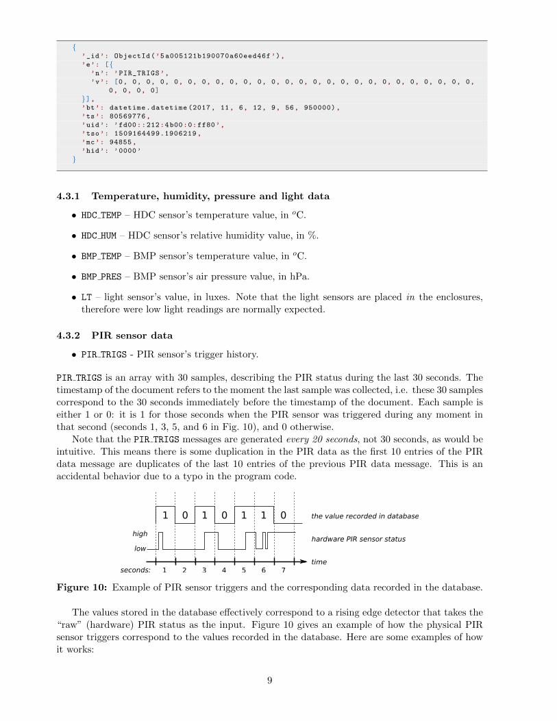
• Appliance monitors (“CurrentCost sensors”, Fig. 8). These sensors are plugged in somewall sockets and record the electricity usage of the attached appliances. These appliances aretypically equipped with sensors: kettle, microwave oven, toaster, TV.

• The SPHERE Genie. This is a tablet computer that allows the user to control the SPHEREsystem, such as to pause the collection of the data. It produces command and notificationmessages.

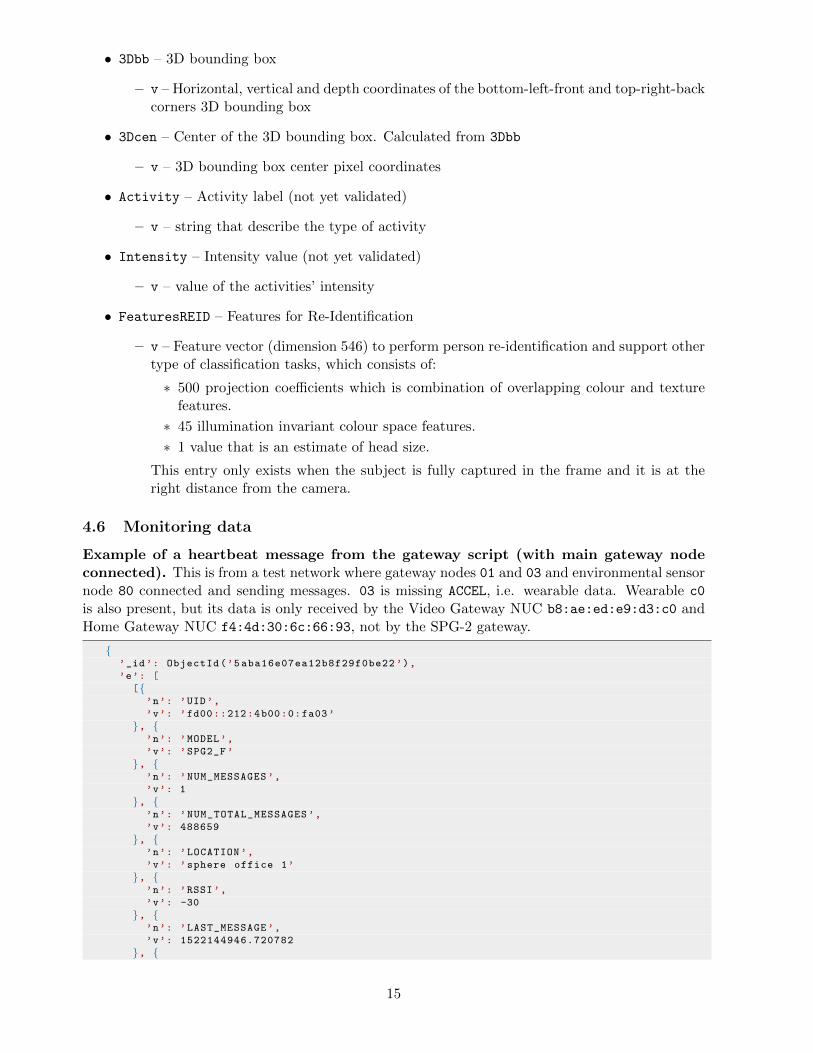
• A SPHERE Home Gateway (Fig. 9). This is a central server that wirelessly collects thedata from the rest of the SPHERE system and stores it in a local, encrypted hard disk. Itproduces no sensor data on its own, but does generate some monitoring data.

3 Architecture

In the SPHERE 100 Homes Study, the SPHERE platform is deployed in residential houses. Insuch a house (see Fig. 1 for an example), all SPHERE devices are connected in a network, or,more accurately, multiple networks, including WiFi, IEEE 802.15.4, and BLE (Bluetooth LowEnergy) networks: see [2, 3, 7] for the details. All data produced by the SPHERE devices iseventually delivered to and stored on the SPHERE Home Gateway (SHG). On the SHG, the datais temporarily stored in a Mongo database. Once per day, the contents of this database are savedas .bson files; these files are then stored on an external hard drive attached to the SHG.

SPHERE uses MQTT (Message Queuing Telemetry Transport) protocol as its backbone pub-lish/subscribe system. The subsystems of SPHERE deliver their data to the database throughActiveMQ MQTT broker that is running on the SPHERE Home Gateway.

The main data and monitoring data sources in SPHERE are the wearables, the environmentalsensors, and the video cameras/gateways. Data from both wearables and environmental sensors aredelivered to the MQTT broker through a gateway script, which takes the sensor data items, putsthem in timestamped JSON documents, and sends the documents to the MQTT broker. The videogateway data does not go through this gateway script: they produce MQTT messages themselves.Other data sources include the appliance electricity consumption sensors. Finally, scripts runningon the SPHERE Home Gateway produce system monitoring data.

4 Data format

SPHERE stores data in JSON (JavaScript Object Notation) documents. The data format in theSPHERE dataset uses SenML (Sensor Markup Language) [10], extended with extra attributeswhere needed.

4.1 General document format

These fields are present at the top level of SPHERE documents:

• hid – house identifier.

• uid – identifier of the component that created this document. Could be an IPv6 address, aMAC address, or a name.

4

• bt – base time: the time this sensor record was created. A UTC timestamp (in some casesadded by the SHG when the data packet is received) compliant with ISO 8601 data elementsand interchange formats.

• id – MongoDB record identifier. Could be used to infer the time when this sensor record wasadded to the database. Usually this time value is slightly later than bt (up to two minutesfor some documents); it should never be earlier than bt.

• ts – timestamp: for details see the note below.

• tso – timestamp offset: for details see the note below.

• mc – “message count”, i.e., sequence number. Note that for some sequence numbers wraparoundscan be observed in SPHERE data: for example, wearable packets have 16-bit sequence num-ber, which wraps around after every 65536 packets.

• e – an array containing sensor data.

• gw – for wearable messages, an array containing data added by the gateways.

• type – document type, e.g. ALERT. Not present for sensor data documents.

4.1.1 Timestamps

There are multiple timestamp-related fields in many documents, for example, ts and tso. Withthese two fields in particular, there are two separate cases:

1. tso is zero. In this case, ts is simply the UNIX timestamp in seconds.

2. tso is nonzero. In this case, ts is expressed in TSCH network ticks (using ≈ 1/100 of asecond as the units), and the tso is the UNIX timestamp (in seconds) of the moment whenthe TSCH network’s time counting was started.

In both cases, the sum of ts and tso fields, if both are present, should be always equal to theUNIX timestamp corresponding to the bt field.

When working with the SPHERE data, one normally does not need to use ts and tso fielddirectly, but can use the bt field instead. The other two fields are there only for timestamp integritychecking and potential restoration purposes; it introduces some redundancy in the data and servesas an extra safety measure.

4.2 Which devices produce which data?

Note that not every message from a device contains all sensors.

• SPW-2 wearable sensor nodes (Fig. 2, SPW2 in the monitoring data)

+ ACCEL

Note that there’s also an array named gw in the documents with ACCEL data. This arraycontains the RSSI information.

• Video NUC (Fig. 4) with associated 3D camera (Fig. 3)

+ RSSI data about messages from wearables.

+ Video data (silhouettes and bounding boxes)

5

Figure 2: SPHERE Wearable node.

Figure 3: SPHERE Video Camera.

Figure 4: SPHERE Video NUC.

Note that raw video data is not retained: only visual features computed and extracted fromthem are retained and stored.

• SPES-2 environmental sensor nodes (Fig. 5, SPES2 in the monitoring data)

+ HDC TEMP

+ HDC HUM

+ BMP TEMP

+ BMP PRES

+ LT

+ PIR TRIGS

• SPES-2 water flow sensor nodes (Fig. 6, SPAQ2 P in the monitoring data – “AQ” standingfor “Aqua”, “P” standing for “piezo”)

+ HDC TEMP

+ HDC HUM

+ BMP TEMP

6

Figure 5: SPHERE Environmental Sensor node.

+ BMP PRES

+ LT

+ PIR TRIGS

+ PIEZO WATER C

+ PIEZO WATER H

Based on the raw sensor values PIEZO WATER C (cold) and PIEZO WATER H (hot) the gatewayscript publishes estimated water flow status in FLOW COLD ON and FLOW HOT ON.

Figure 6: SPHERE Environmental Water Sensor.

• SPG-2 forwarding gateway nodes (Fig. 7, SPG2 F in the monitoring data):

+ HDC TEMP

+ HDC HUM

+ BMP TEMP

+ BMP PRES

+ WEARABLE ADV – internal only, contains wearable acceleration data

• Appliance monitor sensors (Fig. 8)

+ ELEC

• SPG-2 border router nodes (Fig. 9, SPG2 BR in the monitoring data): no sensors, monitoringinformation only.

7

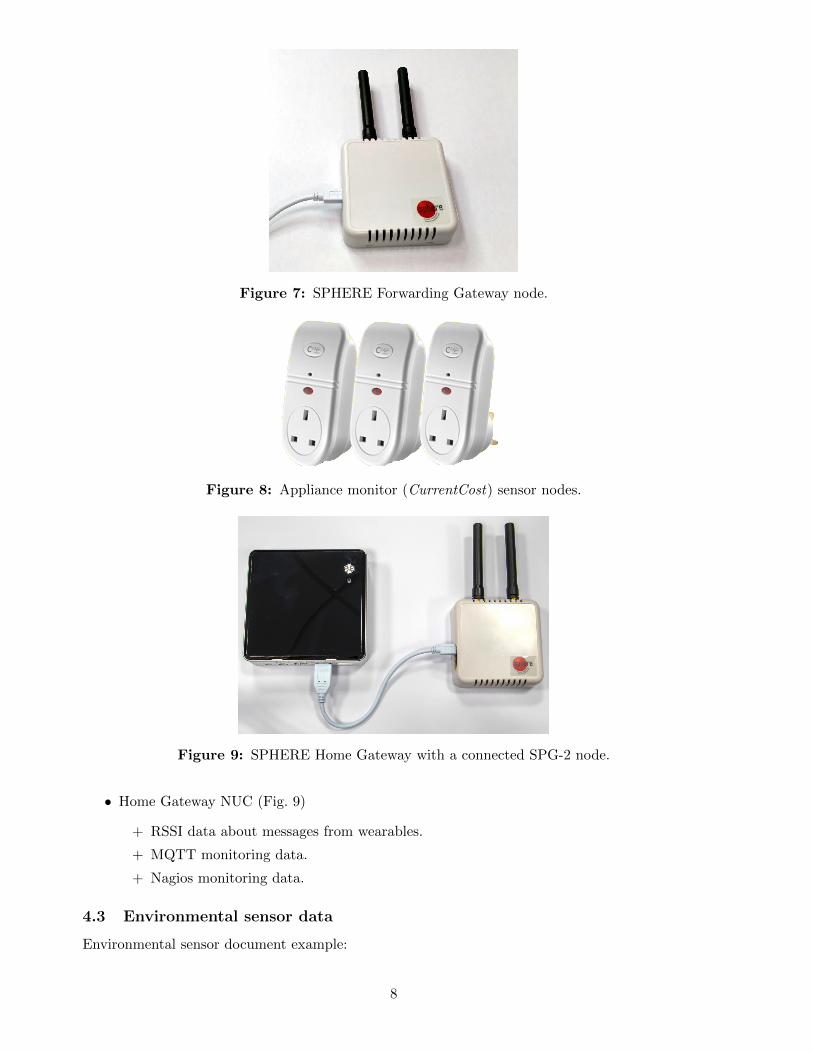
Figure 7: SPHERE Forwarding Gateway node.

Figure 8: Appliance monitor (CurrentCost) sensor nodes.

Figure 9: SPHERE Home Gateway with a connected SPG-2 node.

• Home Gateway NUC (Fig. 9)

+ RSSI data about messages from wearables.

+ MQTT monitoring data.

+ Nagios monitoring data.

4.3 Environmental sensor data

Environmental sensor document example:

8

{’_id’: ObjectId(’5a005121b190070a60eed46f’),

’e’: [{’n’: ’PIR_TRIGS’,

’v’: [0, 0, 0, 0, 0, 0, 0, 0, 0, 0, 0, 0, 0, 0, 0, 0, 0, 0, 0, 0, 0, 0, 0, 0, 0, 0,

0, 0, 0, 0]

}],’bt’: datetime.datetime (2017, 11, 6, 12, 9, 56, 950000),

’ts’: 80569776,

’uid’: ’fd00::212:4b00:0:ff80’,

’tso’: 1509164499.1906219,

’mc’: 94855,

’hid’: ’0000’

}

4.3.1 Temperature, humidity, pressure and light data

• HDC TEMP – HDC sensor’s temperature value, in oC.

• HDC HUM – HDC sensor’s relative humidity value, in %.

• BMP TEMP – BMP sensor’s temperature value, in oC.

• BMP PRES – BMP sensor’s air pressure value, in hPa.

• LT – light sensor’s value, in luxes. Note that the light sensors are placed in the enclosures,therefore were low light readings are normally expected.

4.3.2 PIR sensor data

• PIR TRIGS - PIR sensor’s trigger history.

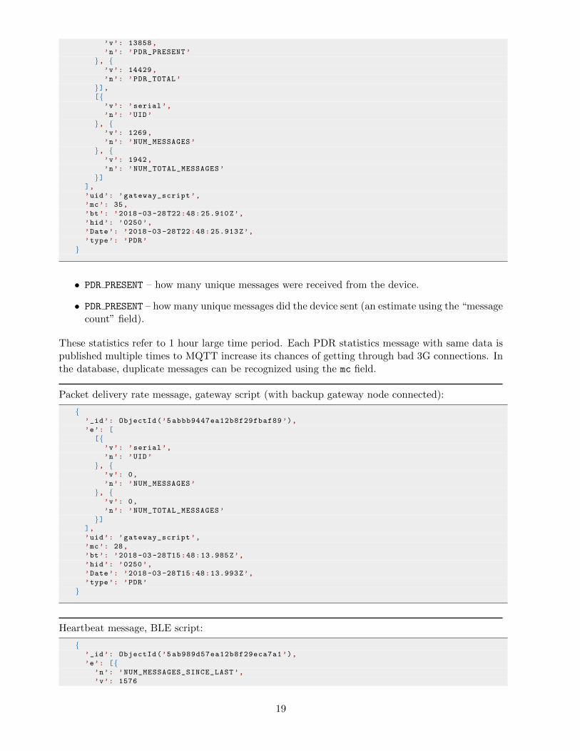
PIR TRIGS is an array with 30 samples, describing the PIR status during the last 30 seconds. Thetimestamp of the document refers to the moment the last sample was collected, i.e. these 30 samplescorrespond to the 30 seconds immediately before the timestamp of the document. Each sample iseither 1 or 0: it is 1 for those seconds when the PIR sensor was triggered during any moment inthat second (seconds 1, 3, 5, and 6 in Fig. 10), and 0 otherwise.

Note that the PIR TRIGS messages are generated every 20 seconds, not 30 seconds, as would beintuitive. This means there is some duplication in the PIR data as the first 10 entries of the PIRdata message are duplicates of the last 10 entries of the previous PIR data message. This is anaccidental behavior due to a typo in the program code.

time1 2 3 4 5 6 7seconds:

hardware PIR sensor status

the value recorded in database

low

high

01 1 1 10 0

Figure 10: Example of PIR sensor triggers and the corresponding data recorded in the database.

The values stored in the database effectively correspond to a rising edge detector that takes the“raw” (hardware) PIR status as the input. Figure 10 gives an example of how the physical PIRsensor triggers correspond to the values recorded in the database. Here are some examples of howit works:

9

• The sensor goes up, then down again: the value in the database is 1 (the 1st second in Fig. 10).

• The sensor goes up and not down: the value in the database is 1 (the 3rd second in Fig. 10).

• The sensor goes down and not up: the value in the database is 0 (the 4th second in Fig. 10).

• The sensor goes up/down multiple times: the value in the database is 1 (the 6th second inFig. 10).

• The value of the hardware PIR sensor is low during the whole second: the value in thedatabase is 0 (the 2nd second in Fig. 10).

• The value of the hardware PIR sensor is high during the whole second: the value in thedatabase is 0 (the 7th second in Fig. 10).

4.3.3 Water flow sensor data

The SPHERE dataset

"Raw" waterflow sensor

data

Binaryclassification

output

SVM classifier

Sensor node withthe flow sensor

hot cold

hot cold

Figure 11: Overview of the water flow sensing subsystem [11]. A piezoelectric sensor is clampedon the water pipe, near the water tap; there is one clamp for the hot water pipe, and one for thecold one. The sensor data is delivered to the SPHERE Home Gateway, where the water flow statusis classified with a machine learning algorithm. Both the raw flow values, the classification results,and the calibration data of the classifier are saved in the dataset.

Raw flow data example:

{’_id’: ObjectId(’5a005075b190070a60eec8cf’),

’e’: [{’n’: ’PIEZO_WATER_C’,

’v’: 13372608

}, {’n’: ’PIEZO_WATER_H’,

’v’: 13380796

}, {’n’: ’LT’,

’v’: 0

}],

10

’bt’: datetime.datetime (2017, 11, 6, 12, 6, 59, 263000),

’ts’: 80552007,

’uid’: ’fd00::212:4b00:0:ff80’,

’tso’: 1509164499.1936808,

’mc’: 94846,

’hid’: ’0000’

}

The architecture of the water flow sensing is given in Fig. 11; for more details consult [11].

• PIEZO WATER C – a 32-bit integer value encapsulating start of reading value (12 bits), end ofreading value(12 bits) and the interrupt status (1 bit) of the cold water flow sensor.

• PIEZO WATER H – a 32-bit integer value encapsulating start of reading value, end of readingvalue and the interrupt status of the hot water flow sensor. The values are encapsulated inthe same way as the values for the cold flow.

Flow classification example:

{’_id’: ObjectId(’5a005075b190070a60eec8cd’),

’uid’: ’fd00::212:4b00:0:ff80’,


’tso’: 1509164499.1936808,

’e’: [{’n’: ’WATER_COLD_ON’,

’v’: False

}, {’n’: ’WATER_HOT_ON’,

’v’: False

}],’ts’: 80552007,

’hid’: ’4954’

}

• WATER COLD ON – a Boolean value describing whether the cold water flow is classified as “on”.

• WATER HOT ON – a Boolean value describing whether the hot water flow is classified as “on”.

These values are only produced if the water sensor calibration process has been successfully com-pleted (each SPHERE house requires separate calibration process).

4.3.4 Appliance monitor data

SPHERE uses the common-off-the-shelf CurrentCost Individual Appliance Monitors (IAMs)1 anda mains meter sensor, called the Energy Transmitter 2, which every 6-7 seconds communicate theirenergy usage data to the NetSmart gateway 3. The CurrentCost gateway is connected via a USB-serial connection using an RJ45 connector on the gateway end. Data transmitted through the serialport to the SHG is picked up by a script that parses and formats each XML packet into JSONand forwards the traffic onto the MQTT queue. Each data packet has some additional informationinserted, such as hid, and the bt of the SHG.Electricity usage message example:

1http://www.currentcost.com/product-iams-specification.html2http://www.currentcost.com/product-transmitter-specifications.html3http://www.currentcost.com/product-netsmart-specification.html

11

{"uid" : "02052",

"bt" : ISODate ("2018 -04 -24 T13:28:19.014+0000"),

"e" : [

{"n" : "ELEC",

"v" : "00013"

}],

"hid" : "9999"

}

• Per device:

– n – sensor name i.e. ’ELEC’.

– v – energy usage value in Watts. This string is actually of integer type of length 5 withleading zeros. The example above denotes an energy consumption of 13 Watts.

Packet timestamps are assigned by the SHG since CurrentCost does not offer an accurate clocksolution for their network – time is reported to a seconds level accuracy and needs to be set manuallyon the gateway.

4.4 Wearable data

Wearable message example:

{’_id’: ObjectId(’5a00512ab190070a60eed598’),

’e’: [{’n’: ’ACCEL’,

’t’: 0.4,

’v’: [0.096, -0.864, -0.064]

}, {’n’: ’ACCEL’,

’t’: 0.32,

’v’: [ -0.096, -0.96, -0.192]

}, {’n’: ’ACCEL’,

’t’: 0.24,

’v’: [ -0.064, -0.96, -0.064]

}, {’n’: ’ACCEL’,

’t’: 0.16,

’v’: [ -0.256, -0.832, -0.256]

}, {’n’: ’ACCEL’,

’t’: 0.08,

’v’: [ -0.256, -1.024, -0.224]

}, {’n’: ’ACCEL’,

’t’: 0,

’v’: [ -0.064, -0.832, -0.032]

}],’bt’: datetime.datetime (2017, 11, 6, 12, 9, 59),

’gw’: [{’uid’: ’fd00::212:4b00:0:ff05’,

’rssi’: -89,

’mc’: 171761,

’ts’: 80569981

}, {’uid’: ’fd00::212:4b00:0:ff03’,

’rssi’: -84,

’mc’: 1691039,

’ts’: 80569982

}, {

12

’uid’: ’fd00::212:4b00:0:ff04’,

’rssi’: -82,

’mc’: 2119128,

’ts’: 80569982

}, {’uid’: ’fd00::212:4b00:0:ff06’,

’rssi’: -84,

’mc’: 2621139,

’ts’: 80569982

}, {’uid’: ’fd00::212:4b00:0:ff07’,

’rssi’: -76,

’mc’: 1885067,

’ts’: 80569983

}],’ts’: 80569981,

’uid’: ’a0:e6:f8:00:ff:c0’,

’tso’: 1509164499.1903248,

’mc’: 44539,

’hid’: ’0000’

}

• ACCEL – acceleration data

– v – the x, y, z coordinates of the acceleration data (always in this order)

– t – the timestamp offset (in seconds) of this data relative to the timestamp of thedocument.

Packet timestamps are assigned by gateways, not wearables, since wearables are not time-synchronizedwith the rest of the SPHERE’s network.

In a wearable data document, the top-level ts field is equal to the smallest of the ts fields insidethe gw array: that is, we treat the timestamp assigned by the gateway that “first” received thepacket as the timestamp of the packet. In the example, the timestamps of the different gateways areslightly different: the maximal timestamp is 0.02 seconds larger than the minimal timestamp. Thisis a very common occurrence; an error of this magnitude is present in ≈ 30 percent on wearablepackets (see the “data quality” section for detailed discussion).

In contrast to timestamps, there are multiple, independent sequence numbers in the wearabledata document. The top-level mc field refers to the sequence number of the wearable that generatedthe acceleration data. In theory, this field can be used to restore higher accuracy timestamps of thewearable data in case the bt field is deemed insufficiently accurate. The mc fields in the elementsof the gw array refer to the sequence numbers of the gateways that forwarded the data.

4.5 Video data

The video data is constituted by two different types of messages: the bounding box informationand the actual silhouette image. Each silhouette image entry is characterized by the first elementof e being the text “silhouette”. This entry contains the png file of the raw silhouette encoded inform of base64. All the entries following the silhouette are bounding boxes, detected by the persondetector. To collect all the bounding boxes detected in a specific frame, it is useful to query thedatabase for elements which have the same base time bt and the same uid (the camera room id)as the specified silhouette frame.

Video message example containing a silhouette∗:

{’_id’: ObjectId(’59 d4f16eb159dd06d20053ac’),


’e’: [{’n’: ’silhouette’,

13

’v’: ’iVBORw0KGgoAAAANSUhEUgAAAoAAAAHgCAAAAAAQuoM4AAAPFElEQVR4Ae3Bi3aiQABEwdtz+

P9f7tUYN5r4AISZAbqKiIiIiIiIi ...’ # base64 format

}],’hid’: u’4954’,

’uid’: u’b8aeed7edc31’

}

∗ To represent the silhouettes, the Base64 format is used. Base64 is a group of similar binary-to-text encoding schemes that represent binary data in an ASCII string format by translating itinto a radix-64 representation. The term Base64 originates from a specific MIME content transferencoding. Each base64 digit represents exactly 6 bits of data. Three 8-bit bytes (i.e., a total of 24bits) can therefore be represented by four 6-bit base64 digits.

Video message example for a bounding box:

{’_id’: ObjectId(’59 d9db1ab190070a60c977c3’),


’e’: [{’n’: ’frameID’,

’v’: 123178

}, {’n’: ’userID’,

’v’: 1089350673

}, {’n’: ’2Dbb’,

’v’: [500, 96, 595, 263]

}, {’n’: ’2DCen’,

’v’: [554, 151]

}, {’n’: ’3Dbb’,

’v’: [1430, 1144, 4533, 2475, -207, 5133]

}, {’n’: ’3Dcen’,

’v’: [1989, 748, 4833]

}, {’n’: ’Activity’,

’v’: u’Sitting Down’

}, {’n’: ’Intensity’,

’v’: u’Light+’

}, {’n’: ’FeaturesREID’,

’v’: [0.4997463822364807, -0.7747822403907776, -2.420274496078491,

0.8493637442588806, 0.151933953166008, 1.3922899961471558, ...]

}],’hid’: ’4954’,

’uid’: ’b8aeed7edc31’}

• frameID – Frame ID

– v – frame ID number.

• userID – User ID

– v – user ID number. Used for tracking bounding boxes while the person appear in theframe

• 2Dbb – 2D bounding box

– v – Horizontal and vertical coordinates of the bottom-left and top-right corners

• 2DCen – Center of the 2D bounding box

– v – 2D bounding box center pixel coordinates. Calculated from 2Dbb

14

• 3Dbb – 3D bounding box

– v – Horizontal, vertical and depth coordinates of the bottom-left-front and top-right-backcorners 3D bounding box

• 3Dcen – Center of the 3D bounding box. Calculated from 3Dbb

– v – 3D bounding box center pixel coordinates

• Activity – Activity label (not yet validated)

– v – string that describe the type of activity

• Intensity – Intensity value (not yet validated)

– v – value of the activities’ intensity

• FeaturesREID – Features for Re-Identification

– v – Feature vector (dimension 546) to perform person re-identification and support othertype of classification tasks, which consists of:

∗ 500 projection coefficients which is combination of overlapping colour and texturefeatures.

∗ 45 illumination invariant colour space features.

∗ 1 value that is an estimate of head size.

This entry only exists when the subject is fully captured in the frame and it is at theright distance from the camera.

4.6 Monitoring data

Example of a heartbeat message from the gateway script (with main gateway nodeconnected). This is from a test network where gateway nodes 01 and 03 and environmental sensornode 80 connected and sending messages. 03 is missing ACCEL, i.e. wearable data. Wearable c0

is also present, but its data is only received by the Video Gateway NUC b8:ae:ed:e9:d3:c0 andHome Gateway NUC f4:4d:30:6c:66:93, not by the SPG-2 gateway.

{’_id’: ObjectId(’5aba16e07ea12b8f29f0be22’),

’e’: [

[{’n’: ’UID’,

’v’: ’fd00::212:4b00:0:fa03’

}, {’n’: ’MODEL’,

’v’: ’SPG2_F’

}, {’n’: ’NUM_MESSAGES’,

’v’: 1

}, {’n’: ’NUM_TOTAL_MESSAGES’,

’v’: 488659

}, {’n’: ’LOCATION’,

’v’: ’sphere office 1’

}, {’n’: ’RSSI’,

’v’: -30

}, {’n’: ’LAST_MESSAGE’,

’v’: 1522144946.720782

}, {

15

’n’: ’MISSING_SENSORS’,

’v’: [’ACCEL’]

}],[{

’n’: ’UID’,

’v’: ’fd00::212:4b00:0:fa80’

}, {’n’: ’MODEL’,

’v’: ’SPES2’


’v’: 2


’v’: 39768



}, {’n’: ’RSSI’,

’v’: -20


’v’: 1522144964.9395883

}],[{

’n’: ’UID’,

’v’: ’fd00::212:4b00:0:fa01’

}, {’n’: ’MODEL’,

’v’: ’SPG2_BR’


’v’: 1


’v’: 34011




’v’: 1522144961.2643692

}],[{

’n’: ’UID’,

’v’: ’a0:e6:f8:00:fa:c0’

}, {’n’: ’MODEL’,

’v’: ’SPW2’


’v’: 494


’v’: 7961121


’v’: ’A’


’v’: 1522144987.4976475

}],[{

’n’: ’UID’,

’v’: ’f4:4d:30:6c:66:93’

}, {’n’: ’MODEL’,

’v’: ’Intel NUC HOME’


’v’: 248

16


’v’: 3542351




’v’: 1522144986.548605

}],[{

’n’: ’UID’,

’v’: ’b8:ae:ed:e9:d3:c0’

}, {’n’: ’MODEL’,

’v’: ’Intel NUC VIDEO’


’v’: 246


’v’: 3493470


’v’: ’sphere office - hall 1’


’v’: 1522144987.4976475

}], {’n’: ’UPTIME’,

’v’: 926114.7416009903

}, {’n’: ’SERIAL_PORT’,

’v’: 1

}, {’n’: ’GW_NODE_ALIVE’,

’v’: 1

}],

’uid’: ’gateway_script’,

’bt’: ’2018 -03 -27 T10:03:08.380Z’,

’hid’: ’0250’,

’Date’: ’2018 -03 -27 T10:03:08.384Z’,

’type’: ’HEARTBEAT’

}

• Per device:

– UID – ID of the device.

– LOCATION – information about the device’s location, if present in HyperCat.

– MODEL – the model of the device.

– NUM MESSAGES – number of messages from the device in the last reporting period (1 min).

– NUM TOTAL MESSAGES –number of messages from the device since the start of the script.

– LAST MESSAGE – the local time when last message was received from the device.

– ERRORS – any specific errors for that node (e.g. invalid environmental sensor readings)since the last heartbeat message.

– NEXTHOP – the node through which this device is connected (only for TSCH devices).

– RSSI – the RSSI of the last packet from the device (only for directly connected TSCHdevices).

– MISSING SENSORS – array of sensors detected as not reported by the device, if any. Forexample, having ACCEL here is normal in case the wearables are not in the communicationrange of the device.

17

• SERIAL PORT – whether the serial port is open.

• GW NODE ALIVE – whether the connected node is communicating.

• UPTIME – the uptime of the script.

Example of a heartbeat message from the gateway script (with backup gateway nodeconnected):

{’_id’: ObjectId(’5aba17027ea12b8f29f0bed9’),

’e’: [{’n’: ’UPTIME’,

’v’: 926147.5098118782

}, {’n’: ’SERIAL_PORT’,

’v’: 1

}, {’n’: ’GW_NODE_ALIVE’,

’v’: 1

}],’uid’: ’gateway_script’,

’bt’: ’2018 -03 -27 T10:03:41.148Z’,

’hid’: ’0250’,

’Date’: ’2018 -03 -27 T10:03:41.153Z’,


}

Packet delivery rate message, gateway script (with main gateway node connected):

{’_id’: ObjectId(’5abc1bbf7ea12b8f29fe08b9’),

’e’: [

[{’v’: ’fd00::212:4b00:0:fa01’,

’n’: ’UID’

}, {’v’: 0,

’n’: ’PDR_PRESENT’

}, {’v’: 0,

’n’: ’PDR_TOTAL’

}],[{

’v’: ’fd00::212:4b00:0:fa03’,

’n’: ’UID’

}, {’v’: 83,


}, {’v’: 83,


}],[{

’v’: ’fd00::212:4b00:0:fa80’,

’n’: ’UID’

}, {’v’: 158,


}, {’v’: 158,


}],[{

’v’: ’a0:e6:f8:00:fa:c0’,

’n’: ’UID’

}, {

18

’v’: 13858,


}, {’v’: 14429,


}],[{

’v’: ’serial’,

’n’: ’UID’

}, {’v’: 1269,

’n’: ’NUM_MESSAGES’

}, {’v’: 1942,

’n’: ’NUM_TOTAL_MESSAGES’

}]],


’mc’: 35,

’bt’: ’2018 -03 -28 T22:48:25.910Z’,

’hid’: ’0250’,

’Date’: ’2018 -03 -28 T22:48:25.913Z’,

’type’: ’PDR’

}

• PDR PRESENT – how many unique messages were received from the device.

• PDR PRESENT – how many unique messages did the device sent (an estimate using the “messagecount” field).

These statistics refer to 1 hour large time period. Each PDR statistics message with same data ispublished multiple times to MQTT increase its chances of getting through bad 3G connections. Inthe database, duplicate messages can be recognized using the mc field.

Packet delivery rate message, gateway script (with backup gateway node connected):

{’_id’: ObjectId(’5abbb9447ea12b8f29fbaf89’),

’e’: [

[{’v’: ’serial’,

’n’: ’UID’

}, {’v’: 0,

’n’: ’NUM_MESSAGES’

}, {’v’: 0,

’n’: ’NUM_TOTAL_MESSAGES’

}]],


’mc’: 28,

’bt’: ’2018 -03 -28 T15:48:13.985Z’,

’hid’: ’0250’,

’Date’: ’2018 -03 -28 T15:48:13.993Z’,

’type’: ’PDR’

}

Heartbeat message, BLE script:

{’_id’: ObjectId(’5ab989d57ea12b8f29eca7a1’),

’e’: [{’n’: ’NUM_MESSAGES_SINCE_LAST’,

’v’: 1576

19

}, {’n’: ’NUM_MESSAGES_TOTAL’,

’v’: 4562

}],’uid’: ’BLE_SCRIPT_b8aeed7db949’,

’bt’: ’2018 -03 -27 T00:01:20.999Z’,

’hid’: ’0000’,

’Date’: ’2018 -03 -27 T00:01:20.998Z’,


}

• NUM MESSAGES TOTAL – number of wearable messages received since the start of the script.

• NUM MESSAGES SINCE LAST – number of wearable messages received since the last report.

Monitoring message, SPG-2 and SPES-2 nodes:

{’_id’: ObjectId(’5a039ae7b190070a602a721e’),

’uid’: ’fd00::212:4b00:0:ff87’,


’tso’: 0,

’e’: [{’n’: ’UPTIME’,

’v’: 2908940

}, {’n’: ’FLASH_STATUS’,

’v’: 1

}, {’n’: ’PROCESS_MAX_EVENTS’,

’v’: 3

}, {’n’: ’REBOOT_REASON’,

’v’: 1

}, {’n’: ’REBOOT_IS_DELIBERATE’,

’v’: 1

}, {’n’: ’NUM_REBOOTS’,

’v’: 17

}, {’n’: ’MAX_STACK_SIZE’,

’v’: 1530

}],’ts’: 151018570392.4064,

’hid’: ’0000’,

’Date’: datetime.datetime (2017, 11, 9, 0, 1, 43, 925000)

}

• UPTIME – uptime of the device.

• FLASH STATUS – nonzero if whether external flash read/write test was successful, zero other-wise.

• PROCESS MAX EVENT – maximal number of events in the Contiki process event buffer.

• MAX STACK SIZE – the maximal size of stack used by the application during the execution sofar.

• REBOOT REASON – the reason code for the last reboot. Consult Texas Instruments CC2650documentation for the meaning of these codes.

20

• REBOOT IS DELIBERATE – nonzero if the last reboot was initialized by the software of thenode, zero otherwise. Reboots are initialized when problems are detected, e.g. no CoAPrequests are received for 2 hours.

• NUM REBOOTS – the total number of reboots in the devices life cycle so far.

Battery voltage monitoring message, SPES-2 nodes:

{’_id’: ObjectId(’5a03c5d4b190070a602c9207’),

’uid’: ’fd00::212:4b00:0:ff85’,


’tso’: 1509164487.6929398,

’e’: [{’n’: ’BATMON_VOLT’,

’v’: 3.585

}],’ts’: 103220436,

’hid’: ’0000’,


}

• BATMON VOLT – battery voltage of the device.

Monitoring message, wearable node:

{’_id’: ObjectId(’5ab989d57ea12b8f29eca79f’),

’tso’: 1520032700.7959356,

’e’: [{’n’: ’BATMON_VOLT’,

’v’: 3.333

}, {’n’: ’UPTIME’,

’v’: 4937677

}],’uid’: ’a0:e6:f8:00:ff:c2’,

’ts’: 207618107,

’bt’: ’2018 -03 -27 T00:01:21.865Z’,

’hid’: ’0000’,

’Date’: ’2018 -03 -27 T00:01:22.325Z’

}

• UPTIME – uptime of the device in seconds.

• BATMON VOLT – battery voltage of the device in volts.

• AXLCONF – accelerometer configuration (i.e. the filter control register, FILTER CTL [12]).

• AXLSTAT – accelerometer status (i.e. the status register, STATUS [12]).

• ERR – error code, shown below.

• CPUTEMP – CPU temperature in oC.

• CPUVDD – CPU voltage in volts.

• SW VERSION – software revision number.

• HW VERSION – hardware revision number (board revision number multiplied by 10).

21

Monitoring message, wearable error codes:

typedef enum

{

ERROR_NO_ERROR =0, // Everything OK

ERROR_AXL0_DEAD , // Accelerometer 0 not responding

ERROR_AXL0_FIFO , // Accelerometer 0 unexpected number of samples in FIFO

ERROR_AXL0_FIFO_FULL , // Accelerometer 0 has full FIFO

ERROR_AXL1_DEAD , // Accelerometer 1 not responding

ERROR_AXL1_FIFO , // Accelerometer 1 unexpected number of samples in FIFO

ERROR_SPI0_FAIL , // Failed to initialize SPI0

ERROR_SPI1_FAIL , // Failed to initialize SPI1

ERROR_FLASH , // Failed to initialize external flash memory

ERROR_ADV_CONFIG , // Failed to configure accelerometer

ERROR_CRYPTO_INIT , // Failed to initialize crypto engine

ERROR_CRYPTO_OP // Failed to encrypt or decrypt

} ERROR_TYPE; // Wearable Error Type

TSCH network’s RSSI strength message:

{’_id’: ObjectId(’5a60923fb190070a60fdd63c’),

’uid’: ’fd00::212:4b00:0:ff04’,


’tso’: 0,

’e’: [{’n’: ’RSSI’,

’v’: -71

}, {’n’: ’CHANNEL’,

’v’: 25

}],’ts’: 151627833517.32825,

’hid’: ’0000’,


}

• RSSI – signal strength value.

• CHANNEL – IEEE 802.15.4 channel on which the message is received.

Link-layer neighbor status message (produced for each active neighbor in the neighbor table):

{’_id’: ObjectId(’5a608e9cb190070a60fda9ce’),

’uid’: ’fd00::212:4b00:0:ff80’,


’tso’: 0,

’e’: [{’n’: ’LINK_NEIGHBOR’,

’v’: ’fd00::212:4b00:0:ff05’

}, {’n’: ’LINK_ETX’,

’v’: 128

}, {’n’: ’LINK_PACKETS_TX_PREVIOUS_HOUR’,

’v’: 671

}, {’n’: ’LINK_PACKETS_ACK_PREVIOUS_HOUR’,

’v’: 541

}, {’n’: ’LINK_PACKETS_RX_PREVIOUS_HOUR’,

’v’: 2337

}],’ts’: 151627740446.8441,

22

’hid’: ’0000’,


}

• LINK NEIGHBOR – the IPv6 address of the neighbor.

• LINK ETX – EWMA of the Expected Transmission Count to the neighbor, multiplied by 128.

• LINK PACKETS TX PREVIOUS HOUR – number of packets transmitted (including duplicates).

• LINK PACKETS ACK PREVIOUS HOUR – number of packets ACKed.

• LINK PACKETS RX PREVIOUS HOUR – number of packets received.

See Contiki 3.x documentation and source code for more details on the ETX value.

TSCH node’s status message:

{’_id’: ObjectId(’5a608ea0b190070a60fdaa0f’),

’uid’: ’fd00::212:4b00:0:ff80’,


’tso’: 1513623272.9585357,

’e’: [{’n’: ’TSCH_OUTGOING_DROPPED’,

’v’: 0

}, {’n’: ’TSCH_INCOMING_DROPPED’,

’v’: 0

}, {’n’: ’TSCH_MAX_SYNC_ERROR’,

’v’: 229

}, {’n’: ’TSCH_HOPPING_SEQUENCE’,

’v’: [12, 14, 13, 25, 20, 11, 16]

}, {’n’: ’TSCH_CHANNEL_IDLE_RSSI’,

’v’: [0, 0, 0, 0, 0, 0, 0, 0, 0, 0, 0, 0, 0, 0, 0, 0]

}, {’n’: ’TSCH_TIMESOURCE’,

’v’: ’fd00::212:4b00:0:ff01’

}, {’n’: ’TSCH_DRIFT’,

’v’: 8.953

}],’ts’: 265413536,

’hid’: ’0000’,


}

• TSCH OUT OK – number of outgoing packets transmitted successfully.

• TSCH OUTGOING DROPPED – number of outgoing packets dropped due to all reasons. Presentonly in SPHERE version D; version E breaks down this to a more detailed information (seefurther).

• TSCH OUT DROPPED TX LIMIT – number of outgoing packets dropped due to exceeded retrans-mission count.

• TSCH OUT DROPPED QUEUE FULL – number of outgoing packets dropped due to full queue.

• TSCH OUT DROPPED NO ROUTE – number of outgoing packets dropped due to not having routeto the destination.

23

• TSCH OUT DROPPED NO NEIGHBOR – number of outgoing packets dropped due to not havingentry for the nexthop in the neighbor tables.

• TSCH OUT DROPPED OTHER – number of outgoing packets dropped due to other reasons.

• TSCH INCOMING DROPPED – number of incoming packets dropped.

• TSCH NUM DISSOCIATIONS – number of times the node has left the TSCH network since thelast reboot.

• TSCH MAX SYNC ERROR – maximal time synchronization error, in microseconds.

• TSCH HOPPING SEQUENCE – the current hopping sequence.

• TSCH CHANNEL IDLE RSSI – background noise RSSI.

• TSCH TIMESOURCE – TSCH time source node’s address (same as RPL routing parent).

• TSCH DRIFT – clock drift estimate, in ppm.

TSCH CHANNEL IDLE RSSI has valid readings only on the root gateway node.

TSCH node’s neighbor status message (produced only for the timesource neighbor):

{’_id’: ObjectId(’5a608ea4b190070a60fdaa29’),

’uid’: ’fd00::212:4b00:0:ff80’,


’tso’: 0,

’e’: [{’n’: ’TSCH_NEIGHBOR’,

’v’: ’fd00::212:4b00:0:3301’

}, {’n’: ’TSCH_HOPPING_SEQUENCE’,

’v’: [12, 14, 13, 25, 20, 11, 16]

}, {’n’: ’TSCH_RSSI’,

’v’: [ -73, -74, -74, -77, -76, -75, -77]

}, {’n’: ’TSCH_LQI’,

’v’: [57, 58, 58, 56, 58, 57, 58]

}, {’n’: ’TSCH_P_TX’,

’v’: [0.92, 1, 1, 1, 1, 1, 0.99]

}],’ts’: 151627741238.31018,

’hid’: ’0000’,


}

• TSCH NEIGHBOR – the neighbor’s IPv6 address.

• TSCH HOPPING SEQUENCE – the TSCH hopping sequence currently used.

• TSCH RSSI – per-channel RSSI values for packets received from that neighbor. EWMA-filtered.

• TSCH LQI – per-channel LQI values for packets received from that neighbor. EWMA-filtered.

• TSCH P TX – the Ptx, successful packet acknowledgement probability from that neighbor.EWMA-filtered values for the channels in the TSCH hopping sequence.

24

Note that these statistics are accurate only for channels that have been used for a sufficiently longtime.

Contiki energest status message:

{’_id’: ObjectId(’5a608eadb190070a60fdaab2’),

’uid’: ’fd00::212:4b00:0:ff80’,


’tso’: 0,

’e’: [{’n’: ’ENERGEST_TYPE_OPT’,

’v’: 499756858

}, {’n’: ’ENERGEST_TYPE_FLASH_STANDBY’,

’v’: 1482

}, {’n’: ’ENERGEST_TYPE_LED_RED’,

’v’: 2794

}, {’n’: ’ENERGEST_TYPE_FLASH_ERASE’,

’v’: 0

}, {’n’: ’ENERGEST_TYPE_FLASH_WRITE’,

’v’: 0

}, {’n’: ’ENERGEST_TYPE_HDC’,

’v’: 94983338

}, {’n’: ’ENERGEST_TYPE_LISTEN’,

’v’: 6477566

}, {’n’: ’ENERGEST_TYPE_LED_YELLOW’,

’v’: 5698

}, {’n’: ’ENERGEST_TYPE_BMP’,

’v’: 95860702

}, {’n’: ’ENERGEST_TYPE_FLASH_READ’,

’v’: 1318

}, {’n’: ’ENERGEST_TYPE_TRANSMIT’,

’v’: 0

}, {’n’: ’ENERGEST_TYPE_LED_GREEN’,

’v’: 5710

}, {’n’: ’ENERGEST_TYPE_DEEP_LPM’,

’v’: 2711035296.0

}, {’n’: ’ENERGEST_TYPE_LPM’,

’v’: 402464618

}, {’n’: ’ENERGEST_TYPE_CPU’,

’v’: 122434880

}],’ts’: 151627742129.8406,

’hid’: ’0000’,


}

Note: this describes only the energy consumption of the system outside TSCH timeslot processing!Radio Tx/Rx time should be inferred for packet Tx/Rx statistics instead.

• ENERGEST TYPE DEEP LPM – number of rtimer ticks spent in deep-sleep mode (0.016µA av-erage current consumption on SPES-2 devices).

• ENERGEST TYPE LPM – number of rtimer ticks spent in sleep mode (1.335µA average currentconsumption on SPES-2 devices).

25

• ENERGEST CPU – number of rtimer ticks spent in active mode (2.703µA average currentconsumption on SPES-2 devices).

The duration of one rtimer on SPHERE platforms is 1/65536 seconds. Normally, the rest ofvalues can be ignored, as in SPHERE they are insignificant compared to the CPU and radio energyconsumption.

Packet count message. This should be used in conjunction with Contiki energest status message toinfer the total energy consumption of the node.

{’_id’: ObjectId(’5a608eb9b190070a60fdab2e’),

’uid’: ’fd00::212:4b00:0:ff80’,


’tso’: 0,

’e’: [{’n’: ’PACKETS_TX_UNICAST’,

’v’: [0, 0, 0, 0, 0, 0, 0, 0, 0, 0, 0, 0, 0, 0, 0, 0, 0, 0, 354, 0, 3535, 0, 356,

915, 0, 707, 0, 4725, 347, 231, 5183, 13609]

}, {’n’: ’PACKETS_TX_BROADCAST’,

’v’: [0, 0, 0, 0, 0, 0, 0, 0, 0, 0, 0, 0, 0, 0, 0, 0, 0, 0, 0, 0, 0, 0, 0, 0, 0, 0,

0, 0, 0, 0, 0, 0]

}],’ts’: 151627743317.7867,

’hid’: ’0000’,


}

• PACKETS TX UNICAST – number of unicast packets transmitted.

• PACKETS TX BROADCAST – number of broadcast packets transmitted.

• PACKETS RX UNICAST – number of unicast packets received (and normally acknowledged).

• PACKETS RX BROADCAST – number of broadcast packets received.

The number of packets is given as an array. Each entry in that array counts number of packets witha specific size: i.e. the first entry counts packets that are 0–3 bytes long, the second for packets4–7 bytes long, and so on.

RPL status message:

{’_id’: ObjectId(’5a608ef0b190070a60fdadd0’),

’uid’: ’fd00::212:4b00:0:ff81’,


’tso’: 0,

’e’: [{’n’: ’RPL_ROOT_REPAIRS’,

’v’: 0

}, {’n’: ’RPL_LOCAL_REPAIRS’,

’v’: 2

}, {’n’: ’RPL_LOOP_ERRORS’,

’v’: 0

}, {’n’: ’RPL_RESETS’,

’v’: 0

}, {’n’: ’RPL_LOOP_WARNINGS’,

’v’: 0

}, {

26

’n’: ’RPL_PARENT_SWITCH’,

’v’: 7

}, {’n’: ’RPL_MEM_OVERFLOWS’,

’v’: 0

}, {’n’: ’RPL_GLOBAL_REPAIRS’,

’v’: 0

}, {’n’: ’RPL_MALFORMED_MSGS’,

’v’: 0

}, {’n’: ’RPL_FORWARD_ERRORS’,

’v’: 0

}],’ts’: 151627748862.37112,

’hid’: ’0000’,


}

This contains various RPL statistics, for more information consult Contiki 3.x documentation andsource code.

IP status message:

{’_id’: ObjectId(’5a60b979b190070a6000475e’),

’uid’: ’fd00::212:4b00:0:ff80’,


’tso’: 0,

’e’: [{’n’: ’IP_FWD’,

’v’: 0

}, {’n’: ’IP_SENT’,

’v’: 28621

}, {’n’: ’IP_CHKERR’,

’v’: 0

}, {’n’: ’IP_RECV’,

’v’: 24013

}, {’n’: ’IP_VHLERR’,

’v’: 0

}, {’n’: ’IP_FRAGERR’,

’v’: 0

}, {’n’: ’IP_PROTOERR’,

’v’: 0

}, {’n’: ’IP_LBLENERR’,

’v’: 0

}, {’n’: ’IP_HBLENERR’,

’v’: 0

}, {’n’: ’IP_DROP’,

’v’: 0

}],’ts’: 151628837795.3567,

’hid’: ’0000’,


}

This contains various IP statistics, for more information consult Contiki 3.x documentation andsource code.

27

Link-layer status message:

{’_id’: ObjectId(’5a60b979b190070a6000475e’),

’uid’: ’fd00::212:4b00:0:ff80’,


’tso’: 0,

’e’: [{’n’: ’LL_TOOLONG’,

’v’: 0

}, {’n’: ’LL_TOOSHORT’,

’v’: 0

}, {’n’: ’LL_BADSYNCH’,

’v’: 0

}, {’n’: ’LL_BADCRC’,

’v’: 0

}, {’n’: ’LL_CONTENTIONDROP’,

’v’: 0

}, {’n’: ’LL_TX’,

’v’: 2610

}, {’n’: ’LL_RX’,

’v’: 1259

}],’ts’: 151628837795.3567,

’hid’: ’0000’,


}

This contains various link-layer statistics, for more information consult Contiki 3.x documentationand source code.

4.7 Alert messages

Gateway script start/stop message example:

{’_id’: ObjectId(’59 d74895e1bce509f7ecf00b’),



’type’: ’ALERT’,

’e’: [{’v’: ’START’,

’n’: ’ACTION’

}],’hid’: ’0000’,


}

• ACTION – either START or STOP, signals that the gateway script has been started or stopped.

• TIMESTAMP RESYNC TIME – the last time when timestamps were synchronized between thegateway script and the TSCH network. The value 0.0 means “never, since the start of thescript”. (This field not present in the example above.)

4.8 Calibration messages

Water sensor calibration data:

28

{’_id’: ObjectId(’59 d769067ea12b738b400908’),

’src’: ’piezo_calibrator’,

’jsonrpc’: ’2.0’,

’dest’: ’gateway_script’,

’id’: ’79388’,

’bt’: ’2017 -10 -06 T12:29:05.782Z’,

’params’: {’PIEZO_HOT_END’: [2190, 2066, 2106, 2135, 2104, 2118, 2188, 2160, 2162, 2184, 2164,

2107, 2173, 2141, 2170, 2119, 2138, 2124, 1995, 1903, 1912, 1904, 1906, 1899,

1923, 1938, 1938, 1952, 1933, 1931, 1936, 1922, 1937, 1901, 1903, 2013, 2035,

2010, 2014, 1998, 1982, 1998, 2005, 2026, 1839, 1968, 1972, 1960, 1985, 1955,

1966, 1962, 2016, 2029, 2009, 2036, 2038, 2029, 1987, 2006, 2016, 1983, 1991,

1993, 1976, 1640, 1637],

’PIEZO_INTERRUPT_PIN’: [0, 0, 0, 0, 0, 0, 0, 0, 0, 0, 0, 0, 0, 0, 0, 0, 0, 0, 0, 1,

1, 1, 1, 1, 1, 1, 1, 1, 1, 1, 1, 1, 1, 1, 1, 0, 1, 0, 1, 1, 0, 1, 1, 1, 1, 1, 1,

1, 1, 1, 1, 1, 1, 1, 1, 1, 0, 1, 1, 1, 1, 1, 1, 1, 1, 2, 2],

’PIEZO_HOT_START’: [1864, 1858, 1857, 1861, 1858, 1858, 1859, 1861, 1862, 1860, 1856

, 1860, 1861, 1863, 1856, 1862, 1858, 1859, 1854, 1763, 1739, 1748, 1738, 1745,

1774, 1794, 1798, 1852, 1745, 1797, 1818, 1797, 1804, 1784, 1761, 1862, 1823,

1858, 1842, 1850, 1863, 1813, 1836, 1839, 1745, 1808, 1809, 1818, 1820, 1786,

1840, 1768, 1858, 1849, 1825, 1802, 1861, 1844, 1828, 1829, 1800, 1794, 1848,

1826, 1799, 1637, 1638],

’PIEZO_GROUND_TRUTH’: [1, 1, 1, 1, 1, 1, 1, 1, 1, 1, 1, 1, 1, 1, 1, 1, 1, 0, 0, 0, 0

, 0, 0, 0, 0, 0, 0, 0, 0, 0, 0, 0, 0, 0, 0, 0, 0, 0, 0, 0, 0, 0, 0, 0, 0, 0, 0,

2, 2, 2, 2, 2, 2, 2, 2, 2, 2, 2, 2, 2, 2, 2, 2, 2, 2, 3, 3],

’PIEZO_COLD_START’: [1810, 1699, 1717, 1737, 1736, 1752, 1749, 1734, 1735, 1744,

1716, 1737, 1699, 1709, 1717, 1712, 1732, 1726, 1696, 1847, 1856, 1862, 1856,

1854, 1854, 1853, 1840, 1852, 1856, 1859, 1836, 1856, 1855, 1851, 1862, 1849,

1853, 1743, 1851, 1856, 1840, 1851, 1856, 1858, 1860, 1862, 1854, 1854, 1861,

1853, 1852, 1851, 1856, 1854, 1853, 1856, 1818, 1850, 1855, 1850, 1851, 1854,

1854, 1853, 1853, 1639, 1639],

’PIEZO_COLD_END’: [1938, 1875, 1835, 1855, 1860, 1870, 1883, 1884, 1909, 1830, 1873,

1886, 1871, 1867, 1867, 1866, 1890, 1828, 1804, 2096, 2081, 2110, 2043, 2066,

2125, 2033, 2033, 2058, 2057, 2072, 2104, 2140, 2101, 2122, 2101, 1986, 1965,

2062, 2042, 2039, 1961, 2038, 1980, 1987, 1977, 2055, 2059, 2091, 2073, 2065,

2029, 2077, 2049, 2066, 2079, 2029, 2050, 1986, 2013, 2120, 1997, 2037, 2024,

2022, 1984, 1639, 1638]

},’Date’: ’2017 -10 -06 T11:29:05.124Z’,

’hid’: ’0000’,

’method’: ’piezo_calibration_set’

}

• PIEZO COLD START – cold flow start values.

• PIEZO COLD END – cold flow end values.

• PIEZO HOT START – hot flow start values.

• PIEZO HOT END – hot flow end values.

• PIEZO INTERRUPT PIN – interrupt status values.

• PIEZO GROUND TRUTH – “ground truth” class labels marked by the technician who calibratedthe sensor upon installation.

4.9 Other data

SPHERE also uses control messages and other ephemeral MQTT messages to exchange commandsand internal data between the system components. However, these messages are not part of thedataset.

29

5 Data quality issues

5.1 Missing data

Data can be missing because of multiple reasons:

• System switched off or paused. If just paused, monitoring data is still going to be present.

• Home Gateway NUC broken or otherwise not recording data in the database. Monitoringdata still may be present.

• A subsystem is not producing data. E.g. the gateway script may be stopped, which meansthat there is going to be neither wearable, nor environmental sensor, nor network monitoringdata.

• A single device is not producing data. E.g. a video NUC switched off or rebooting; videocamera switched off; an environmental sensor has run out of battery; a gateway node is notpowered; a wearable is out of the house.

• A component of a single device is not working. E.g. some of the gateways occasionally stopforwarding wearable data, even though they still produce and forward environmental sensordata.

In a single house, all environmental sensors have somewhat similar battery lifetime. E.g. if a houseloses the first environmental sensor after 6 month operation, it’s likely that by the end of the monthseveral more will follow, and after 2 more months either all sensors are going to be out of battery,or their batteries will have been replaced by SPHERE technicians.

5.2 Transient failures

The SPES-2 and SPG-2 sensor nodes occasionally reboot. Compared to the initial state of theSPHERE hardware platforms that were rebooting many times per day, by the time of the firstpublic deployments this number of reboots is reduced by several orders of magnitude. Still, thereis on average approximately one reboot per node per month.

• Reboot of the main gateway node. This one has the most impact, as data from all of theSPES-2, SPG-2 and SPW-2 nodes is lost for a while. It takes 3 minutes for the other nodesto notice that the old network is gone, and try to start joining the new one. The joining itselfmay take several minutes; the actual time depends on many random factors and can be verydifferent for different nodes.

• Reboot of another SPG-2 node. The data from this node (including SPW-2 data that it issupposed to be forwarding) is lost until the node rejoins the network, which can take up toseveral minutes.

• Reboot of SPES-2 node similarly means it does not produce sensor data until rejoining thenetwork. Since SPES-2 nodes are battery powered, and the join process takes a lot of energy,frequent reboots may affect SPES-2 battery life.

5.3 Timestamps

5.3.1 General notes

In general, it is tricky to produce timestamps that are always correct. A fault in any of these steps(even a transient fault) is going to cause timestamps that are invalid for a while. E.g. when the

30

root gateway node reboots and the time counter of the TSCH network resets, there might be fewdocuments with invalid bt values, corresponding to the old time offset before the restart of theTSCH network.

A good practice when handling SPHERE data is to compare the bt value (created at the datasource) with the Date value (if present – it is only present in monitoring and control data) andthe ObjectID field (created by the MongoDB). The Date field describes the time the data wasreceived by the MQTT broker. From the ObjectID field, the database record creation time can berecovered. If there is a more than a few minutes mismatch for a document, discard that document.Example code:

import calendar

import time

MAX_BT_DIFF = 10 * 60 # the maximal allowed difference of timestamps

# `doc ` is a SPHERE JSON document

bt = doc['bt']objid = doc['_id']. generation_time# convert the value to a GMT timestamp - all SPHERE documents use GMT/UTC timestamps

bt_ts = calendar.timegm(bt.timetuple ())

# convert the `objid ` value to a timestamp

objid_ts = time.mktime(objid.timetuple ())

delta = abs(bt_ts - objid_ts)

if delta > MAX_BT_DIFF:

print('Too big time difference , discarding the document ...')

From analyzing a subset of the data, we estimate that approximately 0.08 % of documents havemismatched timestamps between the sensor network and MQTT time (the bt and Date values),and 0.25 % have mismatched timestamps between MQTT and the Mongo database values (the Dateand ObjectID values).

5.3.2 Time synchronization architecture

The time synchronization architecture in SPHERE is as follows:

• The SPHERE Home Gateway is NTP synced to the University of Bristol time server.

• The other SPHERE components are synced to the SPHERE Home Gateway (the SHG is anNTP server for video NUC).

• The TSCH network has its own time counter. This counter is reset every time the TSCH rootgateway node restarts. (This can happen as often as multiple times per month.) This counteris not synchronized with the SPHERE Home Gateway directly, but an offset is added to thedocuments during their processing on the SPHERE Home Gateway. This offset describes thetime difference between the TSCH network and the UTC time.

5.3.3 Timestamps for environmental sensor data

Timestamps for the environmental sensor data are with resolution of 0.01 seconds. However, sinceenvironmental values change slowly, the timestamp accuracy for these readings in SPHERE is nothigh. For data compression reasons multiple environmental sensor readings can reuse the sametimestamp, as long as the difference between the reading is less or equal to 1 second. (Note thatthis also applies to PIR sensor and water flow sensor readings.)

31

5.3.4 Timestamps for wearable data

The wearable data are time-stamped at the SPHERE Forwarder nodes. The accuracy of thetimestamps are bounded by three types of timing errors (the propagation and processing delays areinsignificant, i.e. less than 1 ms). The first source of timing errors originates from the fact that,in the TI RTOS BLE stack, advertisements are scheduled using a different clock source than theprimary application processor. As a result, the packet generation and the packet transmissions arescheduled with different clocks that drift. This leads to a delay that is bound by the period of theadvertisements which in turn depends on the sampling frequency (i.e., 0.48 seconds at 12.5 Hz and0.24 seconds at 25 Hz). The second source of timing errors is due to queuing delay in the SPHEREForwarders. This delay is measured at 0.05 seconds in the worst case scenario. The last source ofthe timing errors originates from the TSCH timestamps which have 0.01 second granularity.

5.4 Environmental sensor data

• BMP and HDC sensors may stop working or occasionally produce invalid readings. This willbe seen in the dataset as absence of data from that particular sensor or invalid data. One suchcase is that the HDC sensor on some nodes reads 0 instead of the expected raw data value.When this raw value 0 is converted to oC temperature for storing in the JSON document, itends up being equal stored in the database as −40 oC.

• Light sensors and PIRs may become dusty, dirty or get covered by the participant, and stopproducing valid readings or change their dynamic range because of there reasons.

• Light sensors may be exposed to direct sunlight or direct light from indoor data sources.While not a fault as such, this may create unexpected data, as the sensor is supposed torecord ambient light levels. This will not normally happen since the light sensor is inside theenclosure; it may occasionally happen since its close to the openings in the sensor enclosure.

• PIRs may be facing windows; in this case movements of clouds are going to trigger the PIR.Although the technicians are instructed not to place PIRs opposite windows, in some casesit might be unavoidable.

• Temperature sensors of the SPG-2 gateway nodes always report 1–2 oC higher temperaturethan those of SPES-2 nodes. The mechanism of how this happens is not fully clear. Oneworkaround: use only relative temperature values.

• Temperature sensors may be placed near heat source and record their data instead of theambient temperature data. Again, while this is not a fault as such, it may create unexpectedsensor readings.

• The water sensor may be incorrectly calibrated. Some of the SPHERE deployments facedcalibration problems. For those installations, the classification results will be missing, butthe raw water sensor data is going to be recorded in the database anyway.

• The water sensor clamp attachments to water pipes may change over time (e.g., becomeloose), rendering the calibration data unsuitable for results after the change.

One way to work around invalid sensor readings is sanity-checking whether the data falls in rea-sonable bounds. (We do not discard these “invalid” readings as they also could signal that a real,exceptional event has happened in the house.) For example, these values we are using internally:

32

0 oC ≤ HDC TEMP ≤ 50 oC

0 % ≤ HDC HUM ≤ 100 %

0 oC ≤ BMP TEMP ≤ 50 oC

950 hPa ≤ BMP PRES ≤ 1050 hPa

0 lux ≤ LT ≤ 10000 lux

On top of that, median filter can be applied to discard occasional noisy readings. However, wehaven’t detected a significant amount of random errors in the environmental sensor data (unlikethe wearable data).

5.5 Wearable acceleration data

Some of the data gathered from wearables have random errors. Since these error usually affectonly single reading, these values can be filtered out with a median filter. Note that this problem isnot limited to acceleration data; other data created on wearables are affected by this as well, e.g.message sequence numbers and field in monitoring data, such as battery voltage.

Let’s assume the data has been read into a Python iterable. Then one way to apply the medianfilter is:

def median_filter(data):

result = [0] * len(data)

result [0] = data [0]

for i in range(1, len(data) - 1):

result[i] = median(data[i-1], data[i], data[i+1])

result [-1] = data[-1]

return result

The are multiple ways to implement the median() function. On option is to use sorting: returnsorted([a, b, c])[1]. However, sorting the data is not the most optimal way to compute themedian. For three values, this series of explicit if/else statements is a faster and more portablemethod:

def median(a, b, c):

if a > b:

if b > c:

return b # a, b, c

if a > c:

return c # a, c, b

return a # c, a, b

else: # a <= b

if a > c:

return a # b, a, c

if b > c:

return c # b, c, a

return b # c, b, a

Of interest also are circumstances where the median filter is unable to recover from theseissues. Although these are rare events they predominantly occur when packets arrive with lowRSS. Figure 12a shows an example of the corrupted data. This was taken from a period duringwhich the participant was sleeping, and hence we would expect to see data acceleration data toremain relatively steady. However, at approximately 00:14 we can notice an abrupt disturbanceto the signal. We focus only on this segment in Figure 12b and can count that this disturbancepersists for 6 samples. We can conclude then from this these corruptions arise from one receivedpacket since these contain six samples of accelerometer data.

33

27 00:10

27 00:11

27 00:12

27 00:13

27 00:14

27 00:15

27 00:16

27 00:17

27 00:18

27 00:19

27 00:20

bt

3

2

1

0

1

2

3

4 xyz

(a) A 20 minute segment during a sleeping activitywhere the received acceleration has been corrupted(approx at 00:14).

00:13:50

00:13:50

00:13:51

00:13:51

bt

3

2

1

0

1

2

3

4 xyz

(b) A 5 second segment illustrating the effect of theaccelerometer corruption on the received signal. No-tice the corruption begins after 00:13:50 and persistsfor 6 samples.

Figure 12: This figure illustrates the effect of corruptions on the acceleration data.

Since these disturbances are of a large magnitude they may affect the feature representationsthat are necessary for analytics, activity of daily living detection, behavioural monitoring etc.Several techniques may be applied in combatting the effect here. First one can consider filteringthese signals with a low-pass filter since these are predominantly made up of high-frequency dataoutside of the range of human movement. One may also aggregate the data at the packet level andperform anomaly detection on the sequence of received packets and reject data which is consideredanomalous. With the above example in particular, but also with acceleration traces resulting fromnormal activity within the home, the characteristics of the corrupted data are sufficiently large thatany standard anomaly detection techniques will identify the samples as irregular.

5.6 Wearable localization data (RSSI)

5.6.1 SPG-2 recordings

On occasion, a selection of the SPG-2 nodes do not receive any wearable advertisement packets andrequire a manual reboot to resume normal operation. Nodes may be found in the SPHERE datasetwhich do not have advertisement data for a significant portion of the deployment duration, evenwhen wearables were present in the house. Non-reception of wearable advertisement packets doesnot mean that there is a fault with the hardware as the wearable can often be out of communicationrange of a single SPG-2 node. If processed data from the other nodes and other sensors indicatedthat the wearable was co-located in the same room as the non-functioning node, a hardware faultis the most likely explanation.

5.6.2 NUC recordings

The BLE reception quality by the NUCs is significantly poorer than that of the SPG gatewaynodes. Wearable packets are often only received at much shorter ranges and lower rates than thecustom SPG receivers. NUC BLE antennas are embedded within the device, shielded by othercomponents, and designed for communication with peripherals located within a few meters of thedevice. As a result, in some Homes there are few wearable recordings registered on the NUCs.

The data may also get lost on the WiFi connection between the Video NUC and the SPHEREHome Gateway. One of the causes is the variability on the frame rate (see Figure 13), whichare usually caused by the camera sensors’ drivers. Together with other challenging environmentalcauses, this may affect to the long-term transference of packages. To calibrate the cameras withrespect to the changing ambient lighting conditions throughout the day, the NUCs are rebooted atthree different times each day: 06:30, 10:30 and 00:00.

34

A NUC only picks up RSSI data, not acceleration data, as they do not have the decryptionkeys for acceleration data. If a packet has been received only by a NUC and not by any of thegateway nodes, a record is added to the database without the acceleration data (i.e., the e arrayin the document is empty, only gw is filled).

5.6.3 Pitfalls in interpreting RSSI values

The relation between RSSI and location is not straightforward. Indoor environments are usuallymodeled as multipath RF propagation environments, with shadowing, reflections and other non-line-of-sight propagation phenomena taking place.

The following factors affect signal strength; they are ordered by their approximate magnitude:

• The direct distance between the wearable and the receiver, especially in line-of-sight condi-tions.

• Environmental shadowing and reflections. Walls, ceilings and large pieces of furniture willsignificantly alter and inhibit signal propagation. The material of the obstacles has a directinfluence on whether the signal is attenuated or diffracted: e.g. metal causes reflection ordiffraction, the signal is attenuated significantly through brick or stone, but less so throughwood. The building materials of the SPHERE 100 Homes Study houses was captured by thesite-survey visits and we expect that metadata to be available for the users of the SPHEREdataset(s).

• Body shadowing. Signal strength is significantly affected when the wearable is directed awayfrom the receiving node and the wearer’s body blocks the communication path, for example,a participant standing in the same location and rotating 360◦ would register RSSI readingsthat alter significantly, resembling a sine wave curve when plotted.

• Antenna polarization. Changing the angle the wearable is held relative to the receiver’santenna position affects the RSSI. For example, rotating the hand with a wearable aroundit’s axis is going to significantly affect RSSI even if the rest of the body remains still.

• Fading, such as deep fading caused by multipath propagation of the signal. As this typeof fading is frequency-selective, aggregating the signal over multiple frequencies (e.g. withmean() or max() from multiple samples should help to mitigate this issue. Note that theSPHERE dataset does not include information on which frequency a particular message wasreceived along with the RSSI value of that message due to an unfortunate limitation of theTexas Instruments RTOS (Real Time Operating System) BLE (Bluetooth Low Energy) stack.To overcome this, a time window can be selected and appropriate aggregates calculated forthat time bin. A large enough time window will ensures that RSSI values in all of the threeadvertisement frequencies are considered, however there is a trade-off when considering thetime resolution of the participant’s motion or activities.

• A dynamic environment, e.g. closing or opening doors, moving furniture and other householditems all affect the signal strength through changes in signal reflection/propagation environ-ment.

• Random drift over time, possibly caused by the hardware itself. In terms of distance to thetransmitter, this noise behaves as a constant, meaning that it is more likely to be causedby the receiver, not the transmitter. It also means that it affects weak RSSI values muchmore strongly; i.e. the effect from this rarely registers on −50 dBm values RSSI, but can beprevalent on −80 dBm RSSI.

35

• The way the wearable is worn. Wearing it on a tighter strap puts in closer to skin, can changethe assumed propagation characteristics of the wearable antenna when in closer proximity toa significant dielectric like the body.

• External interference from other Bluetooth and other 2.4GHz devices. Early lab tests donot fully indicate the full effect of unwanted transmitting sources, however, from initial tests,there appears to be a slight increase of the standard deviation of the signal.

In contrast, there is no reason to believe that these factors have significant effect on RSSI:

• Battery voltage levels on wearables and other battery-powered devices. The voltage of theradio subsystem is regulated by the CC2650 chip, and is kept stable even when the batteryvoltage goes down.

• Environmental temperature and humidity. The SPHERE networks are deployed in roomconditions, with stable 20 − 30 oC temperature. The humidity levels, in contrast, can bequite variable indoors, but the SPHERE wireless links are too short for this to have significanteffect.

In theory, other causes of RSSI variation may be present, such as the receiver locking in on aspecific channel. In this case it will receive single-frequency signals from the transmitter ratherthan hopping over all available frequencies pseudorandomly. In this case, the aggregate-over-time-window approach would not help, as an impractically long time window would have to be selectedfor calculating the aggregate RSSI. However, the authors believe that this did not occur in theSPHERE dataset.

5.7 Video data

Despite some quality issues described in section 5.6.2 referred to missing packages, the approachesfor extracting the silhouettes and visual features from RGB and Depth are suitable for lightweightdeployment. However, due to the high variability of conditions captured by these sensor data, thereare situations where the quality of visual features and silhouettes are far from accurate. Therefore,this limitation has to be specially taken into account when relying on these features for posterioranalyses.

5.8 Monitoring data

• Wearable: see Section 5.5.

• Some data is published only to MON topics, therefore it is not saved in the RAW MON topics inthe database along with most of the other monitoring data. It is still going to be part of thedata received over the 3G connection. One example of such data is notification message datapublished by BLE scripts (the scripts that pick up wearable advertisements on NUCs).

• Version E adds some new monitoring data fields that are missing in version D, for example,the GW NODE ALIVE field in the gateway script’s heartbeat messages.

6 Conclusion

In this report we describe the data format of the SPHERE dataset, as well as some known dataquality problems and limitations. Our hope is that this document will be useful to those who arelooking to analyze and extract value from the SPHERE dataset, as well as to projects that plan touse SPHERE software or hardware.

36

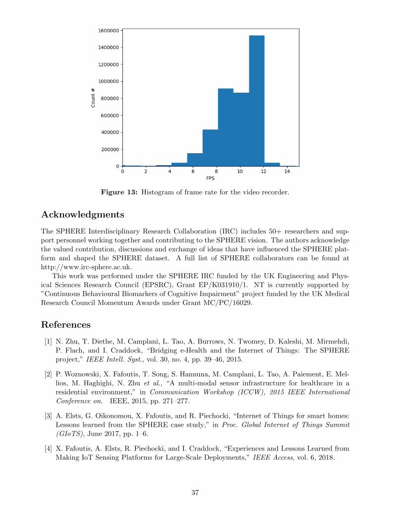
Figure 13: Histogram of frame rate for the video recorder.

Acknowledgments

The SPHERE Interdisciplinary Research Collaboration (IRC) includes 50+ researchers and sup-port personnel working together and contributing to the SPHERE vision. The authors acknowledgethe valued contribution, discussions and exchange of ideas that have influenced the SPHERE plat-form and shaped the SPHERE dataset. A full list of SPHERE collaborators can be found athttp://www.irc-sphere.ac.uk.

This work was performed under the SPHERE IRC funded by the UK Engineering and Phys-ical Sciences Research Council (EPSRC), Grant EP/K031910/1. NT is currently supported by”Continuous Behavioural Biomarkers of Cognitive Impairment” project funded by the UK MedicalResearch Council Momentum Awards under Grant MC/PC/16029.

References

[1] N. Zhu, T. Diethe, M. Camplani, L. Tao, A. Burrows, N. Twomey, D. Kaleshi, M. Mirmehdi,P. Flach, and I. Craddock, “Bridging e-Health and the Internet of Things: The SPHEREproject,” IEEE Intell. Syst., vol. 30, no. 4, pp. 39–46, 2015.

[2] P. Woznowski, X. Fafoutis, T. Song, S. Hannuna, M. Camplani, L. Tao, A. Paiement, E. Mel-lios, M. Haghighi, N. Zhu et al., “A multi-modal sensor infrastructure for healthcare in aresidential environment,” in Communication Workshop (ICCW), 2015 IEEE InternationalConference on. IEEE, 2015, pp. 271–277.

[3] A. Elsts, G. Oikonomou, X. Fafoutis, and R. Piechocki, “Internet of Things for smart homes:Lessons learned from the SPHERE case study,” in Proc. Global Internet of Things Summit(GIoTS), June 2017, pp. 1–6.

[4] X. Fafoutis, A. Elsts, R. Piechocki, and I. Craddock, “Experiences and Lessons Learned fromMaking IoT Sensing Platforms for Large-Scale Deployments,” IEEE Access, vol. 6, 2018.

37

http://www.irc-sphere.ac.uk

[5] X. Fafoutis, A. Vafeas, B. Janko, R. S. Sherratt, J. Pope, A. Elsts, E. Mellios, G. Hilton,G. Oikonomou, R. Piechocki et al., “Designing wearable sensing platforms for healthcare ina residential environment,” EAI Endorsed Transactions on Pervasive Health and Technology,vol. 3, no. 12, 2017.

[6] X. Fafoutis, A. Elsts, A. Vafeas, G. Oikonomou, and R. Piechocki, “Demo: SPES-2 A SensingPlatform for Maintenance-Free Residential Monitoring,” in Proceedings of the EWSN, 2017.

[7] J. Hall, S. Hannuna, M. Camplani, M. Mirmehdi, D. Damen, T. Burghardt, L. Tao,A. Paiement, and I. Craddock, “Designing a video monitoring system for AAL applications:The SPHERE case study,” 2016.

[8] J. Pope, R. McConville, M. Kozlowski, X. Fafoutis, R. Santos-Rodriguez, R. J. Piechocki, andI. Craddock, “SPHERE in a Box: Practical and Scalable EurValve Activity Monitoring SmartHome Kit,” in Proc. 42nd IEEE Conf. Local Computer Networks (LCN) Workshops, 2017.

[9] M. Holmes, H. Song, E. Tonkin, M. P. Nieto, S. Grant, and P. Flach, “Analysis of patientdomestic activity in recovery from Hip or Knee replacement surgery: modelling wrist-wornwearable RSSI and Accelerometer data in the wild,” in Proceedings of The 3rd InternationalWorkshop on Knowledge Discovery in Healthcare Data @IJCAI, Stockholm, Sweden, Jul. 2018,p. 8.

[10] “Internet Draft: Media Types for Sensor Markup Language (SENML),” https://tools.ietf.org/html/draft-jennings-senml-08, 2012.

[11] A. Vafeas, A. Elsts, J. Pope, X. Fafoutis, G. Oikonomou, R. Piechocki, and I. Craddock,“Energy-efficient, noninvasive water flow sensor,” in Proc. SMARTCOMP 2018, 2018.

[12] Analog Devices, “ADXL362 - Micropower, 3-Axis, ±2 g / ±4 g / ±8 g, Digital Output MEMSAccelerometer, Rev. B,” 2013.

38

https://tools.ietf.org/html/draft-jennings-senml-08

https://tools.ietf.org/html/draft-jennings-senml-08

University of Bristol, Faculty of Engineering Technical ...

Documents

Transcript of University of Bristol, Faculty of Engineering Technical ...