University of Alberta - Colorado State University of Alberta ... failure tended to occur in...

University of Alberta

IDENTIFYING HABITATS FOR PERSISTENCE OF

GREATER SAGE-GROUSE (Centrocercus urophasianus)

IN ALBERTA, CANADA

by

Cameron L. Aldridge

A thesis submitted to the Faculty of Graduate Studies and Research in partial fulfillment

of the requirements for the degree of Doctor of Philosophy

in

Environmental Biology and Ecology

Department of Biological Sciences

Edmonton, Alberta

Spring 2005

Abstract

Greater sage-grouse (Centrocercus urophasianus) currently occupy half of their

historic range and populations range-wide have declined by 15-90%. The endangered

Alberta population has declined by as much as 92%, likely a result of reduced

recruitment due to low nest success and poor chick survival. I use spatial modelling

techniques to understand various habitat, climatic, and anthropogenic factors that drive

nest and brood habitat selection, and concurrently assess factors that make habitats

‘risky’ for nests and chicks. At local scales, females recognised ecological cues related to

nest success, selecting for large dense patches of sagebrush with thick grass cover,

placing their nests under moderate density shrubs with suitable obstruction cover from

tall grass. Enhanced nest success resulting from forb cover at all scales, and additional

shrub species at larger scales, however, are ecological cues that are missed, potentially

creating ecological traps. Broods used habitats that were rich in forbs and had moderate

sagebrush cover, tall grass, but less grass cover. Although selection for sagebrush

enhanced chick survival, avoidance of grass dominated areas increased risk. Sage-grouse

may be making tradeoffs between secure-dense cover habitats, and rare forb-rich foraging

habitats that are more open and inherently more risky, particularly in dry years.

Landscape-scale models showed selection for heterogeneous patches of high sagebrush

cover and strong avoidance of anthropogenic edge habitat for nest sites. Similar

heterogeneous high productivity habitats with sagebrush are selected by broods while

avoiding human developments, cropland, and high densities of oil well sites. Chick

failure tended to occur in proximity to oil and gas developments and along riparian

habitats. I predicted these models spatially, identifying source habitats where nests or

chicks were likely to occur and survive, and ‘attractive’ sink habitats where occurrence is

high, but nests fail and chicks die. Ten percent and 5% of the study area was source

habitat, whereas 19% and 15% of habitat was sink habitat for nest and broods,

respectively. My habitat models identified areas that need protection, and habitats that

need immediate management to enhance recruitment and sustain the viability of this

population. I make management recommendations following a collaborative adaptive

management approach.

Acknowledgments

Above all, I must thank my wife. Joanne, your support, your interest, your open

mind and heart, and your loving light-hearted nature have made this whole process easier.

I love you for that, and for always listening to me when I had so much to share; the ups

and the downs. I could not have done this with out you. I also thank my parents, for

encouraging me to follow my dreams, and for allowing me the opportunity to do so.

This research was generously supported financially and/or logistically by the

Alberta Conservation Association, Alberta Cooperative Conservation Research Unit,

Alberta Sustainable Resource Development, Alberta Sport, Recreation, Parks and

Wildlife Foundation, Cactus Communications (Medicine Hat, Alberta), Challenge Grants

in Biodiversity (University of Alberta), Ducks Unlimited Canada (North American

Waterfowl Management Plan), Endangered Species Recovery Fund (World Wildlife

Fund Canada and the Canadian Wildlife Service), Esso Imperial Oil, Manyberries AB,

Murray Chevrolet Medicine Hat AB, and the University of Alberta. I was personally

supported by a University of Alberta Department of Biological Sciences Teaching

Assistantship, a Natural Science and Engineering Research Council Scholarship, a

Macnaughton Conservation Scholarship, an Edmonton Bird Club Scholarship, an

Andrew Stewart Memorial Graduate Prize, the Dorothy J. Killam Memorial Graduate

Prize, an Izaak Walton Killam Memorial Scholarship, the Bill Shostak Wildlife Award,

and the John and Patricia Schlosser Environment Scholarship. Thank you to all for

believing in me, my research, and my conservation efforts.

I thank my advisor, Mark Boyce, for financial support, interest in my research,

and for sharing his ideas and thoughts about science. I have benefited from our

interactions and friendship. I thank my committee members Susan Hannon and Edward

Bork for advice and suggestions throughout my research, and I thank my external

examiners, Michael Gillingham and David Coltman for comments on my thesis. I thank

all of my fellow students in the Alberta Conservation Association Terrestrial Ecosystem

Analysis and Modeling (ACA-TEAM) lab. Our interactions discussing science were

always intriguing; particularly those lunch-time political discussions. Cathy Shier

brought order to the lab and helped to avoid the administrative minefields. My

knowledge about wildlife, statistics, science, academia, and the politics of all, was greatly

advanced from my constant interactions with my good friend Scott Nielsen. I am grateful

for his open door policy fostering our many discussions about science.

I am grateful for endless GIS assistance from Charlene Nielsen and Hawthorne

Beyer, without which, I would still be struggling. Chris Johnson and Jacqui Frair were

always available to discuss survival analyses, and I found solace in having someone to

learn with and from, sharing our ideas. I thank the members of the Mixed Models Club

for our provocative discussions about habitat selection and science in general. Students

have a wealth of knowledge that is often underestimated, yet powerful when united.

I thank Trevor Bush, Jennifer Carpenter, Leah Darling, Craig Dockrill, Quinn

Fletcher, Janet Ng, Maria Olsen, Joanne Saher, Jason Sanders, Danette Sharun, Michael

Swystun, and Megan Watters, for their tireless assistance in the field from someone who

can demand a lot. This thesis would not be possible without each of your contributions.

Roy Penniket (Penniket & Associates Ltd.) produced the sagebrush map product, Ron

McNeil (LandWise Inc.) provided the water impediments layer, Barry W. Adams

(Alberta Public Lands) provided the dry mixedgrass rangeland plant community guide

and great discussions on range management, Lana Robinson, Livio Fent, and Vernon

Ramesz (Alberta Sustainable Resource Development) provided Alberta provincial base

features data, and Arndt Buhlmann and Shad Watts (Alberta Energy) provided the

provincial well site data. Rick Baydack (University of Manitoba) provided information

on the sharp-tailed grouse case study. Dale Eslinger, Joel Nicholson, John Taggart, Ken

Lungle, and Margo Pybus (Alberta Sustainable Resource Development), Paul Jones and

Randy Lee (Alberta Conservation Association) and Bob Fisher (Valley Pet, Medicine

Hat) provided underlying support for my research.

I have spent 8 years living and working in the Manyberries area. Over that time, I

have lived a lot, had some trying times, many friends, and learned much about science,

politics, sociology, and difficult situations. I enjoyed all of it and would not change a

thing. For the landowners that openly allowed me to conduct my research and for those

that always made things interesting, I thank you for your interest, regardless of your

reasons. My research would not have been possible without your support and acceptance

of my work. I thank the following families: the Pearsons, Carrys, Finstads, Murrays,

Kuslers, Schachers, Girards, Heydaluffs, Weeks, Websters, Haugens, Nesmos, Kvales,

Britshgis, Hunters, Piotrowskis, Masers, Gogolinskis, Cravens, Seifreids. Bohnets,

Haugers, Dixons, Yeats, Kleinknects, Hassards, Syversons, Stromsmoes and Wolds, and

individuals: Gerald Maser, Fred Gracey, Hyland Armstrong, Ester Larsen, Esten Larson,

Larry Schlenker, Russell Wegner, Joe Saville, Shelley Benson and Ken Lehr. Access to

community pastures was also pivotal, and I thank the Nemiskam and Manyberries Creek

Community Pastures, the Sage Creek Grazing Association, and the Pinhorn Provincial

Grazing Reserve. Above all, I thank both Peters families for their genuine friendship,

and their open door policy; I sincerely appreciated it.

Table of Contents

CHAPTER ONE .............................................................................................................................................1

General Thesis Introduction ............................................................................................................................1 Literature Cited...........................................................................................................................................7

CHAPTER TWO...........................................................................................................................................13

Predicting Greater Sage-Grouse Nest Occurrence and Survival in Southeastern Alberta: a Fine Scale Approach .......................................................................................................................................................13

1. Introduction ..........................................................................................................................................13 2. Study area .............................................................................................................................................18 3. Methods................................................................................................................................................18

3.1. Field techniques ............................................................................................................................18 3.2. Data Analyses ...............................................................................................................................22

3.2.1. Conditional fixed-effects occurrence analyses......................................................................23 3.2.2. Proportional hazards survival analyses .................................................................................24 3.2.3. Model development...............................................................................................................26 3.2.4. Model selection, assessment and validation..........................................................................27

4. Results ..................................................................................................................................................31 4.1. Candidate models..........................................................................................................................32 4.2. Conditional fixed-effects occurrence analyses..............................................................................34

4.2.1. Nest occurrence at the site scale............................................................................................34 4.2.2. Nest occurrence at the 7.5-m patch radius scale....................................................................36 4.2.3. Nest occurrence at the 15-m radius scale ..............................................................................37

4.3. Proportional hazards survival analyses .........................................................................................38 4.3.1. Survival at the nest site scale.................................................................................................39 4.3.2. Survival at the 7.5-m patch scale ..........................................................................................41 4.3.3. Survival at the 15-m area scale .............................................................................................42

5. Discussion ............................................................................................................................................44 6. Conclusions ..........................................................................................................................................55 7. Literature Cited.....................................................................................................................................85

CHAPTER THREE.......................................................................................................................................92

Greater Sage-Grouse Brood Habitat Selection and Chick Survival in Southeastern Alberta........................92 1. Introduction ..........................................................................................................................................92 2. Study area .............................................................................................................................................95 3. Methods................................................................................................................................................96

3.1. Field techniques ............................................................................................................................96 3.1.1. Chick captures and micro-transmitters..................................................................................96 3.1.2. Habitat measurements ...........................................................................................................98 3.1.3. Brood and chick survival ......................................................................................................99

3.2. Data Analyses ...............................................................................................................................99 3.2.1. Model development.............................................................................................................100 3.2.2. Matched case-control occurrence analyses .........................................................................101 3.2.3. Proportional hazards survival analyses ...............................................................................102 3.2.4. Model selection, assessment and validation........................................................................104

4. Results ................................................................................................................................................107 4.1. Candidate models........................................................................................................................107

4.1.1. Occurrence candidate models..............................................................................................108 4.1.2. Survival candidate models ..................................................................................................109

4.2. Conditional fixed-effects occurrence analyses............................................................................110 4.2.1. Patch scale brood occurrence ..............................................................................................110

4.2.2. Area scale brood occurrence ...............................................................................................112 4.3. Proportional hazards survival analyses .......................................................................................113

4.3.1. Climate chick survival models ............................................................................................114 4.3.2. Shrub chick survival models ...............................................................................................114 4.3.3. Herbaceous chick survival models ......................................................................................115 4.3.4. Combination chick survival models ....................................................................................115

5. Discussion ..........................................................................................................................................118 6. Conclusions ........................................................................................................................................124 7. Literature Cited...................................................................................................................................150

CHAPTER FOUR.......................................................................................................................................157

Linking Occurrence and Fitness: Landscape-scale Nesting and Brood-rearing Habitats for Greater Sage-Grouse in Southeastern Alberta...................................................................................................................157

1. Introduction ........................................................................................................................................157 2. Study area ...........................................................................................................................................162 3. Methods..............................................................................................................................................163

3.1. Field techniques ..........................................................................................................................163 3.2. GIS predictor variables ...............................................................................................................164 3.3. Data Analyses .............................................................................................................................167

3.3.1. Model development.............................................................................................................167 3.3.2. Logistic regression occurrence analyses .............................................................................168 3.3.3. Proportional hazards survival analyses ...............................................................................169 3.3.4. Model assessment and validation........................................................................................170

3.4. Development of habitat states .....................................................................................................171 4. Results ................................................................................................................................................172

4.1. Occurrence models .....................................................................................................................173 4.1.1. Nest occurrence...................................................................................................................173 4.1.2. Brood occurrence ................................................................................................................174

4.2. Proportional hazards survival models .........................................................................................175 4.2.1. Nest survival .......................................................................................................................175 4.2.2. Chick survival .....................................................................................................................176

4.3. Habitat States ..............................................................................................................................177 4.3.1. Nest habitat states................................................................................................................177 4.3.2. Brood habitat states .............................................................................................................178

5. Discussion ..........................................................................................................................................178 5.1. Nesting habitat ............................................................................................................................179 5.2. Brood-rearing habitat ..................................................................................................................183 5.3. Leks as focal points for habitat protection ..................................................................................186

6. Conclusions ........................................................................................................................................187 7. Literature Cited...................................................................................................................................206

CHAPTER FIVE.........................................................................................................................................216

Adaptive Management of Prairie Grouse: How Do We Get There? ...........................................................216 1. Introduction ........................................................................................................................................216 2. History of adaptive management ........................................................................................................217 3. Adaptive management definitions and misconceptions......................................................................218 4. Reasons adaptive management fails ...................................................................................................221 5. Case Study 1: Manitoba sharp-tailed grouse ......................................................................................222 6. Case Study 2: Implementation failures of Alberta sage-grouse adaptive management ......................228 7. Implementation of successful adaptive management .........................................................................233 8. Conclusions ........................................................................................................................................237 9. Literature cited ...................................................................................................................................241

CHAPTER SIX ...........................................................................................................................................245

Thesis Synopsis ...........................................................................................................................................245 Literature Cited.......................................................................................................................................249

List of Tables

Table 2-1. Explanatory variables, means and standard errors (in parentheses) of values used to assess nest fate and occurrence for 93 nest sites and 93 paired random nest locations at three scales in southeastern Alberta from 2001-2003. When grass was absent, height values were considered zero. ............................................................. 58

Table 2-2. Shrub and herbaceous component models used to generate a prior candidate models are shown in (a) for nest site occurrence modeling and survival based on 93 nest sites and 93 paired random nest locations in southeastern Alberta from 2001-2003. Each of the six shrub component models were combined with each of the six herbaceous component models, for a total of 36 different initial candidate models (b). Thirteen models marked asterisk (*) were removed due to violations of the proportional hazards assumption for survival models, leaving 23 candidate models for survival and occurrence modeling....................................................................... 59

Table 2-3. The additional explanatory parameters, means, standard errors (in parentheses) and range of values used to assess nest occurrence for 92 nest sites and 92 paired random nest locations at all three scales in southeastern Alberta from 2001-2003 are shown in a). Observations were not recorded for one nest pair which was dropped. The model structure of additional parameters added to the top AICc-selected model at each scale is shown in b). Note: All models with SBstem violated the proportional hazards assumption, and thus those models were dropped only as candidate survival models. Residual grass (Resid) was highly correlated with grass cover (r >0.70) and was not used in candidate models where the top 2001-2003 AICc-selected model at that scale contained Gr (this was the case for all occurrence models only).............................................................................................................. 60

Table 2-4. AICc-selected nest occurrence models, Akaike weights (wi) for all models comprising a cumulative AICc weight (∑wi) of ≥ 0.90 at the nest site (center quadrat). All model Likelihood Ratio (LR) χ2 tests were significant at P < 0.001. Percent deviance (Dev.) explained indicates the reduction in the log-likelihood from the null model………………………………………………………………………61

Table 2-5. AICc-selected nest occurrence models, Akaike weights (wi) for all models comprising a cumulative AICc weight (∑wi) of ≥ 0.90 for the 7.5-m radius scale from the nest site. All model Likelihood Ratio (LR) χ2 tests were significant at P < 0.001. Percent deviance (Dev.) explained indicates the reduction in the log-likelihood from the null model. ................................................................................ 62

Table 2-6. AICc-selected nest occurrence models, Akaike weights (wi) for all models comprising a cumulative summed AICc weight (∑wi) of ≥ 0.90 for the 15-m radius scale from the nest site. All model Likelihood Ratio (LR) χ2 tests were significant at P < 0.001. Percent deviance (Dev.) explained indicates the reduction in the log-likelihood from the null model. ................................................................................ 63

Table 2-7. Estimated coefficients (βi), standard errors (shown in parentheses), and 95% confidence intervals for top AICc-selected candidate nest occurrence models in south-eastern Alberta for all scales. Models were developed on 93 nest sites and 93 paired random locations collected from 2001-2003. ................................................ 64

Table 2-8. Relative variable importance for nest occurrence models (2001-2003), based on the sum of the AICc weights for each variable across all models. (n=93 nest sites

and 93 paired random locations). Sagebrush variables below the double line illustrate the strength of the measurement technique (quadrats vs. line intercept) and the importance of the quadratic relationship at each scale. Parameter Model Freq. indicates the frequency for each parameter occurring across all 23 models………..65

Table 2-9. Comparison of top AICc-selected nest occurrence models, metrics for overall model significance, fit, and classification accuracy for both training (93 nests from 2001-2003) and testing data (40 nests from 1998-2000) across different scales. All model Likelihood Ratio (LR) χ2 tests were significant at P < 0.001. Percent deviance (Dev.) explained indicates the reduction in the log-likelihood from the null model. The area under the receiver operating characteristic curves [ROC (SE)] and the percent correctly classified (PCC) based on the training dataset optimal cut off point were used to assess model classification accuracy. ......................................... 66

Table 2-10. Nest occurrence models and Akaike weights (wi) for additional parameter models at the nest site (center quadrat) for 92 nests and 92 paired random locations based on the initial 2001-2003 AICc-selected top model (#16). Combinations of additional parameters only measured in 2001-2003 for Robel pole, sagebrush stem cover, and residual grass cover comprised candidate models. All model Likelihood Ratio (LR) χ2 tests were significant at P < 0.001. Percent deviance (Dev.) explained indicates the reduction in the log-likelihood from the null model............................ 67

Table 2-11. Nest occurrence models and Akaike weights (wi) for additional parameter models at the 1st radius (7.5-m scale) for 92 nests and 92 paired random locations based on the initial 2001-2003 AICc-selected top model (#36). Combinations of additional parameters only measured in 2001-2003 for Robel pole, sagebrush stem cover, and residual grass cover comprised candidate models. All model Likelihood Ratio (LR) χ2 tests were significant at P < 0.0001. Percent deviance (Dev.) explained indicates the reduction in the log-likelihood from the null model............................ 68

Table 2-12. Nest occurrence models and Akaike weights (wi) for additional parameter models at the 2nd radius (15-m scale) for 92 nests and 92 paired random locations based on the initial 2001-2003 AICc-selected top model (#25). Combinations of additional parameters only measured in 2001-2003 for Robel pole, sagebrush stem cover, and residual grass cover comprised candidate models. All model Likelihood Ratio (LR) χ2 tests were significant at P < 0.0001. Percent deviance (Dev.) explained indicates the reduction in the log-likelihood from the null model............................ 69

Table 2-13. Estimated coefficients (βi), standard errors (shown in parentheses), and 95% confidence intervals for top AICc-selected additional parameter nest occurrence models for all scales. Models were developed on only 92 of 93 nest and random locations in southeastern Alberta from 2001-2003. Observations were not recorded for one nest pair which was dropped. Added parameters are shown below the dashed line. ............................................................................................................... 70

Table 2-14. Comparison of top AICc-selected nest occurrence models, metrics for overall model significance, model fit, and classification accuracy for the top model with additional parameters (measured for 93 nest and paired random locations from 2001-2003). All model Likelihood Ratio (LR) χ2 tests were significant at P < 0.001 (see previous five tables for scale specifics). Percent deviance (Dev.) explained indicates the reduction in the log-likelihood from the null model. The area under the receiver operating characteristic curves [ROC (SE)] and the percent correctly classified

(PCC) based on the optimal cut off point were used to assess model classification accuracy. An independent sample with these measured parameters was not available, thus, classification statistics are show only for the training (model development) dataset……………………………………………………………….71

Table 2-15. AICc-selected proportional hazards nest survival models, Akaike weights (wi) for all models comprising a cumulative summed AICc weights (∑wi) of ≥ 0.90 at the nest site (center quadrat) for 91 nests from 2001-2003. All model likelihood ratio (LR) χ2 tests were significant at P < 0.005. K indicates the number of model parameters estimates. Percent deviance (Dev.) explained indicates the reduction in the log-likelihood from the null model. .................................................................... 72

Table 2-16. AICc-selected proportional hazards nest survival models, Akaike weights (wi) for all models comprising a cumulative summed AICc weights (∑wi) of ≥ 0.90 for the 7.5-m radius scale from the nest site for 91 nests from 2001-2003. All model likelihood ratio (LR) χ2 tests were significant at P < 0.005. K indicates the number of model parameters estimates. Percent deviance (Dev.) explained indicates the reduction in the log-likelihood from the null model. ................................................ 73

Table 2-17. AICc-selected proportional hazards nest survival models, Akaike weights (wi) for all models comprising a cumulative summed AICc weights (∑wi) of ≥ 0.90 for the 15-m radius scale from the nest site for 91 nests from 2001-2003. All model likelihood ratio(LR) χ2 tests were significant at P < 0.001. K indicates the number of model parameters estimates. Percent deviance (Dev.) explained indicates the reduction in the log-likelihood from the null model. ................................................ 74

Table 2-18. Estimated hazard ratios (exponentiated coefficients - exp[βi]), standard errors (shown in parentheses), and confidence intervals for top AICc-selected candidate proportional hazards nest survival models in south-eastern Alberta across all scales for 91 nests from 2001-2003. Model 22 was the top AICc-selected model for all scales. Note: SBint, SBint2, Gr, and ForbOth did not occur in the top model for any scale. Only at the nest site scale (Model 22-2, right of dashed line) did the top AICc-selected model change with the additional variables (see tables 2-21-2-23). Resid (below dashed line was the only additional variable in Model 22-2. ............. 75

Table 2-19. Relative variable importance for proportional hazards nest survival models (2001-2003), based on the sum of the AICc weights for each variable across all models (91 nest sites). Sagebrush variables below the double line illustrate the strength of the measurement technique (quadrats vs. line intercept) and the importance of the quadratic relationship at each scale. Parameter Model Freq. indicates the frequency for each parameter occurring across all 23 models............. 76

Table 2-20. Comparison of top AICc-selected nest survival models, Akaike weights (wi), and metrics for overall model significance, fit, and classification accuracy for both training (91 nests from 2001-2003) and testing data (38 nests from 1998-2000) across all scales. All model likelihood ratio (LR) χ2 tests were significant at P < 0.001 (see previous five tables for scale specifics). Percent deviance (Dev.) explained indicates the reduction in the log-likelihood from the null model. The area under the receiver operating characteristic curves [ROC (SE)] and the percent correctly classified (PCC) based on the training dataset optimal cut off point were used to assess model classification accuracy. Given that these are hazard survival models, predictions above the cut-off predict failure, below predict survival. Only at

the nest site scale (shown below dashed line) did the top AICc-selected model change with the additional variables (see tables 2-21-2-23). An independent sample for additional variables was not available, thus, classification statistics are shown only for the training (model development) dataset. .................................................. 77

Table 2-21. Proportional hazards nest survival models and Akaike weights (wi) for additional parameter models at the nest site (center quadrat) for 91 nests based on the initial 2001-2003 AICc-selected top model (#22). Combinations of additional parameters only measured in 2001-2003 for Robel pole, sagebrush stem cover, and residual grass cover comprised candidate models. All model likelihood ratio (LR) χ2 tests were significant at P < 0.001. Percent deviance (Dev.) explained indicates the reduction in the log-likelihood from the null model. ................................................ 78

Table 2-22. Proportional hazards nest survival models and Akaike weights (wi) for additional parameter models at the 1st radius (7.5-m scale) for 91 nests based on the initial 2001-2003 AICc-selected top model (#22). Combinations of additional parameters only measured in 2001-2003 for Robel pole, sagebrush stem cover, and residual grass cover comprised candidate models. All model likelihood ratio (LR) χ2

tests were significant at P < 0.001. Percent deviance (Dev.) explained indicates the reduction in the log-likelihood from the null model. ................................................ 79

Table 2-23. Proportional hazards nest survival models and Akaike weights (wi) for additional parameter models at the 2nd radius (15-m scale) for 91 nests based on the initial 2001-2003 AICc-selected top model (#22). Combinations of additional parameters only measured in 2001-2003 for Robel pole, sagebrush stem cover, and residual grass cover comprised candidate models. All model likelihood ratio (LR) χ2 tests were significant at P < 0.001. Percent deviance (Dev.) explained indicates the reduction in the log-likelihood from the null model. ................................................ 80

Table 3-1. Explanatory habitat variables, means and standard errors (in parentheses) of values used to assess brood occurrence and chick survival for 139 brood sites and 139 paired random locations at the patch (177 m2) and area (707 m2) scales in southeastern Alberta from 2001-2003. When grass was absent, height values were considered zero. Models for brood occurrence were initially fit with parameters above the dashed line, validated on an independent set of data from 1998-2000, and then additional parameters only measured for 2001-2003 data were (below dashed line) were added to the top model. Chick survival data was only collected from 2001-2003, and ForbOth was not used in survival models..................................... 126

Table 3-2. Shrub and herbaceous component models used to generate a prior candidate brood occurrence models based on 139 brood sites and 139 paired random nest locations in southeastern Alberta from 2001-2003 at the patch (177 m2) and area (707 m2) scales are shown in (a). Each of the six shrub and herbaceous component models were combined into 36 different initial candidate models (b).................... 127

Table 3-3. Model structure of additional parameters added to the top AICc-selected for brood occurrence modeling. All 139 brood sites and 139 paired random nest locations in southeastern Alberta from 2001-2003 at the patch (177 m2) and area (707 m2) scales were used....................................................................................... 128

Table 3-4. Explanatory climate variables and models used to assess chick survival for 41 radio-marked chicks from 22 different broods in southeastern Alberta from 2001-2003. Due to small sample sizes, a priori climate models consisted of single

parameters only. The asterisk (*) indicates that the GDD model was dropped due to violations of the proportional hazards assumption. ................................................ 129

Table 3-5. Candidate models used to identify the best predictive shrub and herbaceous models predicting sage-grouse chick survival for 41 radio-marked chicks from 22 different broods in southeastern Alberta from 2001-2003. Due to small sample sizes, and in order to develop models with combined components, I limited herbaceous component models to two variables, and modeled each shrub component as a linear or quadratic function. I did not have a validation dataset so parameters withheld from after initial validation for brood occurrence were include in my initial candidate survival models. The asterisk (*) indicates that herbaceous model #12 was dropped due to violations of the proportional hazards assumption. ....................... 130

Table 3-6. AICc brood occurrence models and Akaike weights (wi) for all models within a cumulative summed AICc weight (∑wi) of 0.90 for 139 brood locations at the patch (177 m2) scale. All model Wald χ2 tests were significant at P < 0.0001. Percent deviance (Dev.) explained indicates the reduction in the log-likelihood from the null model. ........................................................................................................ 131

Table 3-7. AICc brood occurrence models and Akaike weights (wi) for all models within a cumulative 90% confidence set (∑wi > 0.90) for 139 brood locations at the area (707 m2) scale. All model Wald χ2 tests were significant at P < 0.0001. Percent deviance (Dev.) explained indicates the reduction in the log-likelihood from the null model....................................................................................................................... 132

Table 3-8. Estimated coefficients (βi), standard errors (shown in parentheses), and 95% confidence intervals for top AICc-selected candidate brood occurrence models in southeastern Alberta. Models were developed on 139 brood sites and 139 paired random locations collected from 2001-2003. ......................................................... 133

Table 3-9. Relative variable importance for brood occurrence models (2001-2003), based on the sum of the AICc weights for each variable across all models. (n=139 brood sites and 139 paired random locations). Sagebrush variables below the double line illustrate the strength of the measurement technique (quadrat vs. line intercept) and the importance of the quadratic relationship at each scale. Parameter Model Frequency indicates the frequency for each parameter occurring across all 36 models. .................................................................................................................... 134

Table 3-10. Comparison of top AICc-selected brood occurrence models, metrics for overall model significance, model fit, and classification accuracy for both training (139 brood sites from 2001-2003) and testing data (113 brood sites from 1998-2000) across different scales. All model Wald χ2 tests were significant at P < 0.0001. Percent deviance (Dev.) explained indicates the reduction in the log-likelihood from the null model. The area under the receiver operating characteristic curves [ROC (SE)] and the percent correctly classified (PCC) based on the training dataset optimal cut off point were used to assess model classification accuracy. .............. 135

Table 3-11. Brood occurrence models and Akaike weights (wi) for additional parameter models at the patch (177 m2) scale for 139 brood and 139 paired random locations based on the initial 2001-2003 AICc-selected top model (#10). Combinations of additional parameters only measured in 2001-2003 for Robel pole, residual grass (Resid) cover, and Litter estimates comprised candidate models. All model Wald χ2

tests were significant at P < 0.0001. Percent deviance (Dev.) explained indicates the reduction in the log-likelihood from the null model. .............................................. 136

Table 3-12. Brood occurrence models and Akaike weights (wi) for additional parameter models at the area (707 m2) scale for 139 brood and 139 paired random locations based on the initial 2001-2003 AICc-selected top model (#10). Combinations of additional parameters only measured in 2001-2003 for Robel pole, residual grass (Resid) cover, and Litter estimates comprised candidate models. All model Wald χ2

tests were significant at P < 0.0001. Percent deviance (Dev.) explained indicates the reduction in the log-likelihood from the null model. .............................................. 137

Table 3-13. AICc-selected climate variable proportional hazards chick survival models and Akaike weights (wi) for 41 chicks from 2001-2003. The Wald χ2 is an estimate of the fit of the model to the data, and K indicates the number of model parameters estimated, which includes the covariates and the estimate of the random effect (Theta). Theta is the estimate of the shared frailty variance and the P value for the likelihood ratio tests (LR) for the significance of the correlation is presented. Percent deviance (Dev.) explained indicates the reduction in the log-likelihood from the null model. ........................................................................................................ 138

Table 3-14. AICc-selected shrub variable proportional hazards chick survival models and Akaike weights (wi) for all models at the 177 m2 patch and 707 m2 area scales for 41 chicks from 2001-2003 in southeastern Alberta. The Wald χ2 indicated the fit of the model to the data, and K indicates the number of model parameters estimated, which includes the covariates and the estimate of the random effect (Theta). Theta is the estimate of the shared frailty variance and the P value for the likelihood ratio tests (LR) for the significance of the correlation is presented. Percent deviance (Dev.) explained indicates the reduction in the log-likelihood from the null model. ........ 139

Table 3-15. AICc-selected herbaceous variable proportional hazards chick survival models and Akaike weights (wi) for all models at the 177 m2 patch scale for 41 chicks from 2001-2003 in southeastern Alberta. The Wald χ2 indicated the fit of the model to the data, and K indicates the number of model parameters estimated, which includes the covariates and the estimate of the random effect (Theta). Theta is the estimate of the shared frailty variance and the P value for the likelihood ratio tests (LR) for the significance of the correlation is presented. Percent deviance (Dev.) explained indicates the reduction in the log-likelihood from the null model. ........ 140

Table 3-16. AICc-selected herbaceous variable proportional hazards chick survival models and Akaike weights (wi) at the 707 m2 area scale for 41 chicks from 2001-2003. The Wald χ2 indicated the fit of the model to the data, and K indicates the number of model parameters estimated, which includes the covariates and the estimate of the random effect (Theta). Theta is the estimate of the shared frailty variance and the P value for the likelihood ratio tests (LR) for the significance of the correlation is presented. Percent deviance (Dev.) explained indicates the reduction in the log-likelihood from the null model. .............................................................. 141

Table 3-17. Overall combined candidate proportional hazards chick survival models for 41 radio-marked chicks from 22 different broods at the patch (177 m2) and area (707 m2) scales in southeastern Alberta from 2001-2003. The top Climate, Shrub, and Herbaceous (Herb) models were used at each scale for combination models. The top within each group was also considered as candidate models within this set. The

model with the combination of ‘sagebrush’ + Dry_Index would not converge on a Maximun Likelihood estimate and was therefore not estimated. ........................... 142

Table 3-18. AICc-selected combined proportional hazards chick survival models and Akaike weights (wi) for all models at the 177 m2 patch and 707 m2 area scales for 41 chicks from 2001-2003 in southeastern Alberta. The Wald χ2 indicated the fit of the model to the data, and K indicates the number of model parameters estimated, which includes the covariates and the estimate of the random effect (Theta). Theta is the estimate of the shared frailty variance and the P value for the likelihood ratio tests (LR) for the significance of the correlation is presented. Percent deviance (Dev.) explained indicates the reduction in the log-likelihood from the null model. ........ 143

Table 3-19. Estimated hazard ratios (exponentiated coefficients - exp[βi]), standard errors (shown in parentheses), and confidence intervals for top AICc-selected candidate proportional hazards chick survival combined models in south-eastern Alberta for 41 chicks from 22 different broods from 2001-2003. The top combined model at both scales had the Dry Index, the Gr + GrHgt Herbaceous component model, and a sagebrush component. ....................................................................... 144

Table 3-20. Relative variable importance for proportional hazards combination chick survival models (2001-2003), based on the sum of the AICc weights for each variable across all models (41 chicks). Parameter Model Freq. indicates the frequency for each parameter occurring across all 6 models.................................. 145

Table 4-1. Explanatory GIS raster variables used for 3rd order sage-grouse occurrence and survival models for sage-grouse nests and broods. All variables were first tested univariately in occurrence (logistic regression) and survival (proportional hazards) models. Candidate variables with P < 0.25 were removed, and correlated variables with higher P-values were removed. Data type refers to continuous (cont.) or categorical (cat.) variables. All distance measures are in km. ............................... 190

Table 4-2. Estimated coefficients (βi) and standard errors (S.E.) for the final nest occurrence model for 113 sage-grouse nests in southeastern Alberta from 2001-2004. 5,000 random points were used to characterise habitat availability and these points were weighted using importance weights such that the available sample was effectively 113 points. P values indicated the significance of the coefficients using a Wald z statistic........................................................................................................ 192

Table 4-3. Estimated coefficients (βi) and standard errors (S.E.) for the final brood occurrence model for 669 sage-grouse brood locations in southeastern Alberta from 2001-2004. 5,000 random points were used to characterise habitat availability and these points were weighted using importance weights such that available sample was effectively 669 points. P values indicated the significance of the coefficients using a Wald z statistic. ....................................................................................................... 192

Table 4-4. Estimated hazard ratios (exponentiated coefficients - exp[βi]) and standard errors (S.E.) for the final proportional hazards nest survival model using 111 sage-grouse nest sites in southeastern Alberta from 2001-2004. P values indicated the significance of the coefficients using a Wald z statistic. ........................................ 193

Table 4-5. Estimated hazard ratios (exponentiated coefficients - exp[βi]) and standard errors (S.E.) for the shared frailty final proportional hazards chick survival model using 41 sage-grouse chicks from 22 different broods in southeastern Alberta from

2001-2003. P values indicated the significance of the coefficients using a Wald z statistic. The shared Frailty variance estimate was θ = 1.246, P = 0.047. ............. 193

List of Figures

Figure 2-1. Kaplan Meier cumulative survival estimates and 95% confidence intervals for 91 sage-grouse nests during incubation in southeastern Alberta from 2001-2003. Six nests abandoned due to inclement weather events were right-censored. ........... 81

Figure 2-2. Threshold response curves for the top AICc-selected model (#22-2) at the nest site (center quadrat) for relative risk (hazard) of nest failure for sage-grouse nests in southern Alberta. Responses are shown across the 90th percentile of availability for each parameter in the model while holding the other parameters in the model at their mean values; a) bush, b) grass height, c) forb cover, and d) residual grass cover. Values below the optimal cut-off threshold (0.2687) indicate reduced hazard, and predicted nest survival. ............................................................ 82

Figure 2-3. Threshold response curves for the top AICc-selected model (#22) at the 7.5-m radius for relative risk (hazard) of nest failure for sage-grouse nests in southern Alberta. Responses are shown across the 90th percentile of availability for each parameter in the model while holding the other parameters in the model at their mean values; a) bush, b) grass height, and c) forb cover. Values below the optimal cut-off threshold (0.2976) indicate reduced hazard, and predicted nest survival. .... 83

Figure 2-4. Threshold response curves for the top AICc-selected model (#22) at the 15-m radius for relative risk (hazard) of nest failure for sage-grouse nests in southern Alberta. Responses are shown across the 90th percentile of availability for each parameter in the model while holding the other parameters in the model at their mean values; a) bush, b) grass height, and c) forb cover. Values below the optimal cut-off threshold (0.2380) indicate reduced hazard, and predicted nest survival. .... 84

Figure 3-1. Comparison of Kaplan Meier cumulative survival curves with 95% confidence intervals for 26 different sage-grouse broods and 41 radio-marked chicks in southeastern Alberta from 2001-2003. The 41 chicks were from 22 different broods, and chick survival shown here does not take into account the correlation between chicks within a brood (maximum of two chicks marked per brood were marked). .................................................................................................................. 146

Figure 3-2. Kaplan Meier (KM) cumulative chick survival curves for 41 radio-marked sage-grouse chicks from 22 different broods in southeastern Alberta from 2001-2003. The basic KM curve (solid line) does not take into account the correlation of marked chicks within the same brood, whereas the Frailty Model (dashed line) represents that baseline Cox proportional hazard survival (i.e. no covariates) and accounts for lack of independence of siblings within the same brood. 95% confidence intervals could not be generated for the frailty model due to the conditional nature of the Cox model on covariates within the model. ................... 147

Figure 3-3. Threshold response curves for the top AICc-selected model (combined Model #5) at the patch scale (177 m2) for relative risk (hazard) for sage-grouse chicks in southern Alberta. Responses are shown across the 90th percentile of availability for each parameter in the model while holding the other parameters in the model at their mean values; a) grass cover, b) grass height, and c) dryness index........................ 148

Figure 3-4. Threshold response curves for the top AICc-selected model (combined Model #6) at the area scale (707 m2) for relative risk (hazard) for sage-grouse chicks in southern Alberta. Responses are shown across the 90th percentile of availability for

each parameter in the model while holding the other parameters in the model at their mean values; a) sagebrush cover estimated with the line intercept method b) grass cover, c) grass height, and d) dryness index. .......................................................... 149

Figure 4-1. Alberta greater sage-grouse study area showing sagebrush density with roads, trails, well pads, and major water bodies. Inset map shows the study area and current range of sage-grouse within Alberta, with major rivers, water bodies, and cities for reference................................................................................................... 194

Figure 4-2. A graphic representation of nesting and brood-rearing habitat states for sage-grouse in southeastern Alberta. States include non-critical (low occurrence) habitat, Primary Habitat (high occurrence and low- moderate risk), Secondary Habitat (good occurrence and low-moderate risk), Primary Sink (high occurrence and moderate-extreme risk), and Secondary Sink (high occurrence and moderate-extreme risk). Adapted from Nielsen (2005). ................................................................................ 195

Figure 4-3. Relative index of sage-grouse nest occurrence in southeastern Alberta, as determined by a logistic regression nest occurrence model. Good and high index values indicate that sage-grouse are likely to nest in these habitats. ...................... 196

Figure 4-4. Area-adjusted frequency of sage-grouse nest sites in southeastern Alberta falling within nest habitat index of occurrence bins ranked as poor, low, moderate, good, and high. Training data consists of 113 within sample nest sites from 2001-2004 and the Validation sample consists 40 out-of-sample nest sites from 1998-2000......................................................................................................................... 197

Figure 4-5 Relative index of sage-grouse brood occurrence in southeastern Alberta, as determined by a logistic regression brood occurrence model. Good and high index values indicate that sage-grouse are likely to raise their broods in these habitats. . 198

Figure 4-6. Area-adjusted frequency of sage-grouse brood sites from southeastern Alberta falling within brood habitat index of occurrence bins ranked as poor, low, moderate, good, and high. Training data consists of 669 within sample brood sites from 2001-2004 and the validation sample consists 151 out-of-sample brood sites from 1998-2000. ..................................................................................................... 199

Figure 4-7. Relative index risk of sage-grouse nest failure in southeastern Alberta, as determined by Cox proportional hazards modelling of nest survival. High and extreme risk values indicated a nest is likely to fail if it occurs in these habitats. . 200

Figure 4-8. Relative index risk of sage-grouse chick failure in southeastern Alberta, as determined by Cox proportional hazards modelling of chick survival. High and extreme risk values indicated chicks are likely to die if hens move their broods into these habitats. .......................................................................................................... 201

Figure 4-9. Nesting habitat states for sage-grouse in southeastern Alberta. Non-critical habitat indicates sage-grouse are not likely to nest in those areas. Primary and secondary indicate high and good likelihood of nest occurrence, respectively, and habitats are areas with minimal-low risk of nest failure, whereas sinks are areas with moderate-extreme risk. For example, primary habitat indicates areas where nests are likely to occur (high occurrence values) and be successful (minimal-low risk values), whereas primary sink indicates high occurrence where nests are likely to fail (moderate-extreme risk values). ....................................................................... 202

Figure 4-10. Nest habitat states that would be included if a 3.2-km radius buffer around all known lek sites was used to protect sage-grouse nesting habitat, as outlined by

Connelly et al. (2000). The 1-km radius buffer represents current protective notations or recommended guidelines used by the province of Alberta to protect critical sage-grouse nesting habitat. The 3.2-km buffer includes 53.9% of Primary and Secondary nesting habitat, whereas the 1-km buffer protects only 9.9% of critical nesting habitat. ............................................................................................ 203

Figure 4-11. Brood habitat states for sage-grouse in southeastern Alberta. Non-critical habitat indicates sage-grouse are not likely to nest in those areas. Primary and secondary indicate high and good likelihood of brood occurrence, respectively, and habitats are areas with minimal-low risk of chick failure, whereas sinks are areas with moderate-extreme risk. For example, primary habitat indicates areas where broods are likely to occur (high occurrence values) and survive (minimal-low risk values), whereas primary sink indicates high occurrence where chicks are likely to fail (moderate-extreme risk values). ....................................................................... 204

Figure 4-12. Brood habitat states that would be included if a 3.2-km radius buffer around all known lek sites was used to protect sage-grouse nesting habitat, as outlined by Connelly et al. (2000). The 1-km radius buffer represents current protective notations or recommended guidelines used by the province of Alberta to protect critical sage-grouse brood-rearing habitat. The 3.2-km buffer includes 62.5% of primary and secondary brood-rearing habitat, whereas the 1-km buffer protects only 9.9% of critical brood habitat.................................................................................. 205

Chapter One

General Thesis Introduction

Greater sage-grouse (Centrocercus urophasianus; hereafter ‘sage-grouse’) have

been studied for over 100 years, with early research focusing on the lek mating system

and behavioural questions (Bond 1900; Scott 1942; Patterson 1952; Eng 1961; Eng

1963). As the 1970s approached, a shift in research to more applied research

management questions began, addressing population estimation and lek attendance

(Dalke et al. 1963; Jenni and Hartzler 1978; Emmons and Braun 1984), hunter harvests

(Braun 1979; Braun 1984; Braun and Beck 1985), and habitat requirements (Klebenow

and Gray 1968; Eng and Schladweiler 1972; Wallestad 1975; Connelly et al. 1981). This

culminated in the development of management guidelines for the maintenance of sage-

grouse habitats (Braun et al. 1977), later revised in 2000 (Connelly et al. 2000).

Combined with observed population declines (Dalke et al. 1963; Connelly and Braun

1997; Braun 1998), this information resulted in significant research on sage-grouse

habitat requirements (Dunn and Braun 1986; Gregg et al. 1994; Fischer et al. 1996;

Aldridge and Brigham 2002; Knick et al. 2003), population dynamics across various life

stages (Connelly et al. 1993; Schroeder 1997; Johnson and Braun 1999; Aldridge and

Brigham 2001; Zablan et al. 2003) and more recently, genetics related research (Young et

al. 2000; Benedict et al. 2003; Taylor et al. 2003).

Sage-grouse inhabit shrub-steppe ecosystems, which have undergone major

changes during the past 100 years, resulting in habitat loss, fragmentation, and

degradation (Knick et al. 2003; Connelly et al. 2004). As a result, sage-grouse currently

1

occupy half of their historic range (Schroeder et al. 2004) and all populations have

declined, ranging between 15-90% (Connelly and Braun 1997; Braun 1998; Connelly et

al. 2004). Today, the abundance and quality of remaining habitats are threatened by a

diverse suite of influences, including conversion of native habitats to agriculture

(Connelly et al. 2004), invasion of habitats by non-native plant species (Knick et al.

2003; Connelly et al. 2004), energy extraction activities and developments (Braun et al.

2002; Lyon and Anderson 2003), intense grazing pressures (Beck and Mitchell 2000;

Hayes and Holl 2003; Crawford et al. 2004), and even global climate change (Thomas et

al. 2004).

The relationship between patterns of grazing, energy developments, human

infrastructure (roads, rural encroachment, etc.) and sage-grouse habitat requirements,

have important management ramifications. Threshold responses across various life-

history stages can greatly assist management of these habitats for viable populations of

sage-grouse, particularly in light of the unpredictable threat that West Nile virus (Naugle

et al. 2004) poses to small populations. Given that population declines have been linked

to poor nesting success (Schroeder et al. 1999; Aldridge and Brigham 2001; Connelly et

al. 2004) and low chick survival (Aldridge 2001; Burkepile et al. 2002), management

aimed at improving habitat quality for nesting and brood rearing are likely to have the

greatest benefits for declining populations.

Species-habitat relationships have become an increasing priority in the field of

conservation biology (Boyce and McDonald 1999; Morrison 2001; Brotons et al. 2004;

Engler et al. 2004). Simply predicting the occurrence of animals across habitats can be

useful, but only if occurrence (or abundance) is somehow positively correlated with

2

fitness (Tyre et al. 2001; Breininger and Carter 2003; Bock and Jones 2004). I define

high-quality habitats to be those where animals are likely to occur (high abundance) but

also have high fitness (reproduction and survival; Van Horne 1983; Morrison 2001).

Conservation biology still struggles to make this crucial link between resources and

fitness (Franklin et al. 2000; Morrison 2001; Bock and Jones 2004; Larson et al. 2004;

Nielsen et al. 2005), often only addressing where animals occur. Wildlife-habitat

management and research should assess both occurrence and fitness. Although much

research on sage-grouse has focused on habitat occurrence relationships, or habitat-

survival relationships (primarily for sage-grouse nesting habitat), limited work has

described how resources influence both occurrence and fitness across multiple life stages.

Based on trends within their currently occupied range, the Alberta sage-grouse

population has declined 66-92% since the 1970s (Aldridge and Brigham 2001, 2003).

Between 400 to 600 birds remain in the population, which is classified as endangered

both provincially and federally (Aldridge and Brigham 2003). While agricultural

expansion in the 1970s appears to have isolated Alberta sage-grouse from more southern

populations (Aldridge and Brigham 2003), the current landscape is heavily fragmented by

roads, power lines, and associated oil and gas activities (Braun, et al. 2002; Aldridge and

Brigham 2003). All habitat occurs within the xeric dry mixedgrasss ecosystem and

grazing is the dominant land use practice (Adams et al. 2004). An increased frequency of

extended drought conditions (Aldridge and Brigham 2002) and the introduction of West

Nile virus (Naugle et al. 2004) pose additional threats to the viability of this endangered

population. Similar to other populations of sage-grouse, reduced recruitment due to low

nest success and poor chick survival has been identified as limiting for this population

3

(Aldridge and Brigham 2001; 2002; 2003) and long-term habitat management initiatives

may be required to improve recruitment and ensure populations remain viable.

The goal of this thesis was to develop models to provide land managers with tools

to identify habitats where sage-grouse are abundant and have high fitness (source

habitats; Pulliam 1988; Hobbs and Hanley 1990; Breininger et al. 1998), as well as

identify habitats in which birds are also likely to occur, but have poor fitness (‘attractive

sink’ habitats; Delibes et al. 2001; Breininger and Carter 2003; Larson et al. 2004). I

used empirical models to understand occurrence and fitness-habitat relationships for

sage-grouse in Alberta. I assessed these habitat relationships from 2001-2004 in a core

use area (1,100 km2) within the 4,000 km2 range of sage-grouse in southeastern Alberta.

I developed models at various local and landscape scales for nests and chicks, the two

most critical life stages for sage-grouse (Aldridge 2001; Crawford et al. 2004). I used

resource selection functions (RSFs; Manly et al. 2002) to develop occurrence models and

I used Cox proportional hazards models (Cox 1972; Andersen and Gill 1982) to develop

survival models. Depending on the scale, life stage, and model type, I considered a

variety of different habitat, climate, and anthropogenic variables for inclusion in each

model. With the exception of the chick survival models, I had an independent set of data

collected within this same study area from 1998-2000, which I used to validate all models

and assess model predictive capacity.

In chapter 2, I modeled nest occurrence using local vegetation characteristics

selected by females (4th order; Johnson 1980) at three scales surrounding the nest site. I

developed survival models using local vegetation characteristics that best predict nest

failure/survival at each scale. In chapter 3, I took a similar approach, assessing 4th order

4

habitat selection by sage-grouse broods and chick survival using habitat variables as well

as several climate covariates. In that chapter, I also introduced the use of shared-frailty

proportional-hazards models (Therneau et al. 2003; Wintrebert et al. 2005) to account for

a lack of independence of chicks within broods, and compared these models to more

traditional ‘brood’ survival and chick flush count methods. In both chapter 2 and 3, I

used these models to identify vegetation thresholds, above which sage-grouse are likely

to be successful.

In chapter 4, I used similar modeling approaches, but used a Geographic

Information System (GIS) to model landscape scale habitat and anthropogenic features

linked to both nest and brood occurrence and nest and chick survival. I used these

models to identify various habitat states, depicting habitats which are likely to be

‘sources’ and in need of protection, and habitats which are likely to be ‘attractive’ sinks

resulting in ecological traps (Bock and Jones 2004; Battin 2004) that will require

management. Finally, I evaluated the effectiveness of current sage-grouse habitat

management initiatives, using the recommended 3.2-km habitat-protection buffer around

lek sites (Connelly et al. 2000) and the 1-km protection buffer currently employed within

the province of Alberta.

In chapter 5, I discuss recent failures to implement collaborative adaptive

management strategies for the Alberta sage-grouse population and a population of sharp-

tailed grouse (Tympanuchus phasianellus) in Manitoba, highlighting the challenges that

lie ahead. That chapter was recently published in the Wildlife Society Bulletin (Aldridge

et al. 2004). Finally, in chapter 6, I summarise all of my findings, bringing together these

5

results within the context of management requirements for sage-grouse in general, and

more specifically, within the context of the Alberta population.

6

Literature Cited

Adams, B.W., J. Carlson, D. Milner, T. Hood, B. Cairns, and P. Herzog. Beneficial grazing management practices for sage-grouse (Centrocercus urpohasianus) and ecology of silver sagebrush (Artemisia cana) in southeastern Alberta. 2004. Technical Report, Public Lands and Forest Division, Alberta Sustainable Resource Development. Pub No. T/049.

Aldridge, C.L. 2001. Do sage grouse have a future in Canada? Population dynamics and management suggestions. Pages 1-11 in Anonymous eds. Proceedings of the 6th Prairie Conservation and Endangered Species Conference; 22-25 February 2001, Winnipeg, Manitoba, Canada

Aldridge, C.L., M.S. Boyce, and R.K. Baydack. 2004. Adaptive management of prairie grouse: how do we get there? Wildlife Society Bulletin 32: 92-103.

Aldridge, C.L. and R.M. Brigham. 2001. Nesting and reproductive activities of greater sage-grouse in a declining northern fringe population. Condor 103: 537-543.

Aldridge, C.L. and R.M. Brigham. 2002. Sage-Grouse nesting and brood habitat use in southern Canada. Journal of Wildlife Management 66: 433-444.

Aldridge, C.L. and R.M. Brigham. 2003. Distribution, abundance, and status of the greater sage-grouse, Centrocercus urophasianus, in Canada. Canadian Field-Naturalist 117: 25-34.

Andersen, P.K. and R.D. Gill. 1982. Cox regression-model for counting-processes - a large sample study. Annals of Statistics 10: 1100-1120.

Battin, J. 2004. When good animals love bad habitats: ecological traps and the conservation of animal populations. Conservation Biology 18: 1482-1491.

Beck, J.L. and D.L. Mitchell. 2000. Influences of livestock grazing on sage grouse habitat. Wildlife Society Bulletin 28: 993-1002.

Benedict, N.G., S.J. Oyler-Mccance, S.E. Taylor, C.E. Braun, and T.W. Quinn. 2003. Evaluation of the eastern (Centrocercus urophasianus urophasianus) and western (Centrocercus urophasianus phaios) subspecies of sage-grouse using mitochondrial control-region sequence data. Conservation Genetics 4: 301-310.

Bock, C.E. and Z.F. Jones. 2004. Avian habitat evaluation: should counting birds count? Frontiers in Ecology and the Environment 2: 403-410.

Bond, F. 1900. A nuptial performance of the sage cock. Auk 17: 325-327.

Boyce, M.S. and L.L. McDonald. 1999. Relating populations to habitats using resource selection functions. Trends in Ecology and Evolution 14: 268-272.

7

Braun, C.E. 1979. Evaluation of the effects of changes in hunting regulations on sage grouse populations. Denver, Colorado Division of Wildlife. P-R Proj. W-37-R-32, Job 9a.

Braun, C.E. 1984. Attributes of a hunted sage grouse population in Colorado, U.S.A. Pages 148-162 in P.J. Hudson and T.W.I. Lovel (eds.). 3rd International Grouse Symposium. 1984. World Pheasant Association. York University, Yorkshire, UK.

Braun, C.E. 1998. Sage grouse declines in western North America: what are the problems? Proceedings of the Western Association of State Fish and Wildlife Agencies 78: 139-156.

Braun, C.E. and T.D.I. Beck. 1985. Effects of changes in hunting regulations on sage grouse harvest and populations. Pages 335-343 in S.L. Beasom and S.F. Roberson (eds.). Game harvest management. Proceedings of the 3rd International Symposium. Kingsville, Texas, Caesar Kleberg Research Institute.

Braun, C.E., T. Britt, and R.O. Wallestad. 1977. Guidelines for maintenance of sage grouse habitats. Wildlife Society Bulletin 5: 99-106.

Braun, C.E., O.O. Oedekoven, and C.L. Aldridge. 2002. Oil and gas development in western North America: effects on sagebrush steppe avifauna with particular emphasis on sage grouse. Transactions of the North American Wildlife and Natural Resources Conference 67: 337-349.

Breininger, D.R. and G.M. Carter. 2003. Territory quality transitions and source-sink dynamics in a Florida scrub-jay population. Ecological Applications 13: 516-529.

Breininger, D.R., V.L. Larson, B.W. Duncan, and R.B. Smith. 1998. Linking habitat suitability to demographic success in Florida scrub-jays. Wildlife Society Bulletin 26: 118-128.

Brotons, L., W. Thuiller, M.B. Araujo, and A.H. Hirzel. 2004. Presence-absence versus presence-only modelling methods for predicting bird habitat suitability. Ecography 27: 437-448.

Burkepile, N.A., J.W. Connelly, D.W. Stanley, and K.P. Reese. 2002. Attachment of radiotransmitters to one-day-old sage grouse chicks. Wildlife Society Bulletin 30: 93-96.

Connelly, J.W., W.J. Arthur, and O.D. Markham. 1981. Sage grouse leks on recently disturbed sites. Journal of Range Management 34: 153-154.

Connelly, J.W. and C.E. Braun. 1997. Long-term changes in sage grouse Centrocercus urophasianus populations in western North America. Wildlife Biology 3: 229-234.

Connelly, J.W., R.A. Fischer, A.D. Apa, K.P. Reese, and W.L. Wakkinen. 1993. Renesting by sage grouse in southeastern Idaho. Condor 95: 1041-1043.

8

Connelly, J.W., S.T. Knick, M.A. Schroeder, and S.J. Stiver. 2004. Conservation assessment of greater sage-grouse and sagebrush habitats. Western Association of Fish and Wildlife Agencies, Cheyenne, Wyoming, USA.

Connelly, J.W., M.A. Schroeder, A.R. Sands, and C.E. Braun. 2000. Guidelines to manage sage grouse populations and their habitats. Wildlife Society Bulletin 28: 967-985.

Crawford, J.A., R.A. Olson, N.E. West, J.C. Mosley, M.A. Schroeder, T.D. Whitson, R.F. Miller, Gregg M.A., and C.S. Boyd. 2004. Synthesis paper - ecology and management of sage-grouse and sage-grouse habitat. Journal of Range Management 57: 2-19.

Dalke, P.D., D.B. Pyrah, D.C. Stanton, J.E. Crawford, and E.F. Schlatterer. 1963. Ecology, Productivity and management of sage grouse in Idaho. Journal of Wildlife Management 27: 810-841.

Delibes, M., P. Gaona, and P. Ferreras. 2001. Effects of an attractive sink leading into maladaptive habitat selection. American Naturalist 158: 277-285.

Dunn, P.O. and C.E. Braun. 1986. Summer habitat use by adult female and juvenile sage grouse. Journal of Wildlife Management 50: 228-235.

Emmons, S.R. and C.E. Braun. 1984. Lek attendance of male sage grouse. Journal of Wildlife Management 48: 1023-1028.

Eng, R.L. 1961. Sage grouse-spring strutting activity. Naturalist 2: 15-20.

Eng, R.L. 1963. Observations on the breeding biology of male sage grouse. Journal of Wildlife Management 27: 841-846.

Eng, R.L. and P. Schladweiler. 1972. Sage grouse winter movements and habitat use in Central Montana. Journal of Wildlife Management 36: 141-146.

Engler, R., A. Guisan, and L. Rechsteiner. 2004. An improved approach for predicting the distribution of rare and endangered species from occurrence and pseudo-absence data. Journal of Applied Ecology 41: 263-274.

Fischer, R.A., K.P. Reese, and J.W. Connelly. 1996. An investigation of fire effects within xeric sage grouse brood habitat. Journal of Range Management 49: 194-198.

Franklin, A.B., D.R. Anderson, R.J. Gutierrez, and K.P. Burnham. 2000. Climate, habitat quality, and fitness in northern spotted owl populations in northwestern California. Ecological Monographs 70: 539-590.

Gregg, M.A., J.A. Crawford, M.S. Drut, and A.K. DeLong. 1994. Vegetational cover and predation of sage grouse nests in Oregon. Journal of Wildlife Management 58: 162-166.

9

Hayes, G.F. and K.D. Holl. 2003. Cattle grazing impacts on annual forbs and vegetation composition of mesic grasslands in California. Conservation Biology 17: 1694-1702.

Hobbs, N.T. and T.A. Hanley. 1990. Habitat evaluation - do use availability data reflect carrying-capacity. Journal of Wildlife Management 54: 515-522.

Jenni, D.A. and J.E. Hartzler. 1978. Attendance at a sage grouse lek: implications for spring censuses. Journal of Wildlife Management 42: 46-52.

Johnson, D.H. 1980. The comparison of usage and availability measurements for evaluating resource preference. Ecology 61: 65-71.

Johnson, K.H. and C.E. Braun. 1999. Viability of an exploited sage grouse population. Conservation Biology 13: 77-84.

Klebenow, D.A. and G.M. Gray. 1968. Food habits of juvenile sage grouse. Journal of Range Management 21: 80-83.

Knick, S.T., D.S. Dobkin, J.T. Rotenberry, M.A. Schroeder, W.M. Vander Haegen, and C. Van Riper. 2003. Teetering on the edge or too late? Conservation and research issues for avifauna of sagebrush habitats. Condor 105: 611-634.

Larson, M.A., F.R. Thompson, J.J. Millspaugh, W.D. Dijak, and S.R. Shifley. 2004. Linking population viability, habitat suitability, and landscape simulation models for conservation planning. Ecological Modelling 180: 103-118.

Lyon, A.G. and S.H. Anderson. 2003. Potential gas development impacts on sage grouse nest initiation and movement. Wildlife Society Bulletin 31: 486-491.

Manly, B.F.J., L.L. McDonald, D.L. Thomas, T.L. McDonald, and W.P. Erickson. 2002. Resource selection by animals: statistical design and analysis for field studies. Chapman & Hall, London.

Morrison, M.L. 2001. Invited Paper: A proposed research emphasis to overcome the limits of wildlife-habitat relationship studies. Journal of Wildlife Management 65: 613-623.

Naugle, D.E., C.L. Aldridge, B.L. Walker, T.E. Cornish, B.J. Moynahan, M.J. Holloran, K. Brown, G.D. Johnson, E.T. Schmidtmann, R.T. Mayer, C.Y. Kato, M.R. Matchett, T.J. Christiansen, W.E. Cook, T. Creekmore, R.D. Falise, E.T. Rinkes, and M.S. Boyce. 2004. West Nile virus: pending crisis for greater sage-grouse. Ecology Letters 7: 704-713.

Nielsen, S.E., C.J. Johnson, D.C. Heard, and M.S. Boyce. 2005. Can models of presence-absence be used to scale abundance? Two case studies considering extremes in life history. Ecography 28: 1-12.

Patterson, R.L. 1952. The sage grouse in Wyoming. Sage Books, Inc, Denver CO.

10

Pulliam, H.R. 1988. Sources, sinks, and population regulation. American Naturalist 132: 652-661.

Schroeder, M.A. 1997. Do sage grouse Centrocercus urophasianus exhibit metapopulations in north-central Washington, USA? Wildlife Biology 3: 269.

Schroeder, M.A., C.L. Aldridge, A.D. Apa, J.R. Bohne, C.E. Braun, S.D. Bunnell, J.W. Connelly, P.A. Deibert, S.C. Gardner, M.A. Hilliard, G.D. Kobriger, S.M. Mcadam, C.W. Mccarthy, J.J. Mccarthy, D.L. Mitchell, E.V. Rickerson, and S.J. Stiver. 2004. Distribution of sage-grouse in North America. Condor 106: 363-376.

Schroeder, M.A., J.R. Young, and C.E. Braun. 1999. Sage Grouse (Centrocercus urophasianus). Page 28 in A. Pool and F. Gill, eds. The birds of North America. The Birds of North America, Inc, Philadelphia, Pennsylvania, USA.

Scott, J.W. 1942. Mating behaviour of the sage grouse. Auk 59: 477-498.

Taylor, S.E., S.J. Oyler-Mccance, and T.W. Quinn. 2003. Isolation and characterization of microsatellite loci in greater Sage-Grouse (Centrocercus Urophasianus). Molecular Ecology Notes 3: 262-264.

Therneau, T.M., P.M. Grambsch, and V.S. Pankratz. 2003. Penalized survival models and frailty. Journal of Computational and Graphical Statistics 12: 156-175.

Thomas, C.D., A. Cameron, R.E. Green, M. Bakkenes, L.J. Beaumont, Y.C. Collingham, B.F.N. Erasmus, M.F. De Siqueira, A. Grainger, L. Hannah, L. Hughes, B. Huntley, A.S. Van Jaarsveld, G.F. Midgley, L. Miles, M.A. Ortega-Huerta, A.T. Peterson, O.L. Phillips, and S.E. Williams. 2004. Extinction risk from climate change. Nature 427: 145-148.

Tyre, A.J., H.P. Possingham, and D.B. Lindenmayer. 2001. Inferring process from pattern: can territory occupancy provide information about life history parameters? Ecological Applications 11: 1722-1737.

Van Horne, B. 1983. Density as a misleading indicator of habitat quality. Journal of Wildlife Management 47: 893-901.

Wallestad, R.O. 1975. Life history and habitat requirements of sage grouse in central Montana. Montana Department of Fish, Game, and Parks, Helena, Montana, USA.

Wintrebert, C.M.A., A.H. Zwinderman, E. Cam, R. Pradel, and J.C. Van Houwelingen. 2005. Joint modelling of breeding and survival in the kittiwake using frailty models. Ecological Modelling 181: 203-213.

Young, J.R., C.E. Braun, S.J. Oyler-Mccance, J.W. Hupp, and T.W. Quinn. 2000. A new species of sage-grouse (Phasianidae: Centrocercus) from Southwestern Colorado. Wilson Bulletin 112: 445-453.

11

Zablan, M.A., C.E. Braun, and G.C. White. 2003. Estimation of greater sage-grouse survival in North Park, Colorado. Journal of Wildlife Management 67: 144-154.

12

Chapter Two

Predicting Greater Sage-Grouse Nest Occurrence and Survival in Southeastern

Alberta: a Fine Scale Approach

1. Introduction

Understanding species-habitat relationships, and thus, predicting species

occurrence or density has become an increasing priority in the field of conservation

biology (Boyce and McDonald 1999; Morrison 2001; Brotons et al. 2004; Engler et al.

2004; Nielsen et al. 2005), particularly for threatened and endangered species.

Occurrence is often thought of as a surrogate measure of habitat quality. In 1983, van

Horne proposed that habitat quality should be defined as the product of density

(probability of occurrence), survival probability, and expectation of future offspring

(fecundity), or what she referred to as “mean individual fitness per unit area”. Thus,

‘habitat quality’ assessments based on occurrence alone are missing the crucial link to

survival or overall fitness (Van Horne 1983; Tyre et al. 2001; Breininger and Carter

2003) and have been shown to be a poor indicator of survival (Van Horne 1983; Hobbs

and Hanley 1990; Tyre et al. 2001). Despite the passing of more than 20 years of

conservation and wildlife science since van Horne’s (1983) seminal discussion of how,

and what, constitutes good measures of ‘habitat quality’, the field of ecology is still

struggling to make the link between resources and fitness (Franklin et al. 2000; Morrison

2001; Bock and Jones 2004; Larson et al. 2004; Nielsen et al. 2005).

Occurrence or density estimates often lack information about the mechanisms of

habitat selection and quality, are unlinked to fitness measures, and ultimately, may be

13

uninformative about population persistence. As Morrison (2001) clearly pointed out in

his review on the limits of wildlife-habitat relationships; “we repeatedly fail to find

commonalities in ‘habitat’ for most populations across space because we usually miss the

underlying mechanisms…determining occupancy, survival and fecundity.” He further

noted that the surrogates that we continually use are simply ‘hit-and-miss’ attempts to

statistically model wildlife-habitat relationships (Morrison 2001). Including fitness

measures in habitat modeling is of paramount importance for conservation of threatened

and endangered species. Without the link between occurrence and fitness, surrogate

‘habitat quality’ models using occurrence only, could naively result in the

implementation of inappropriate management strategies.

Suitable measures of fitness for many wildlife species are often difficult to obtain,

due to the long-lived nature of those species. Sample sizes are often an issue when

working with rare or endangered species, limiting our ability to understand variability

around those parameters. Nonetheless, one should still strive to find measures of

fecundity and survival that link to species’ resource needs and ensure population

viability, the ultimate goal of conservation biology. Spatially explicit habitat-based

population-viability analysis linking resources to population demographics has proven to

be a promising tool for understanding animal-habitat relationships, whether modelling

finer scale mechanisms ( Franklin et al. 2000; Johnson et al. 2001) or large scale

surrogates in a Geographic Information System (Akcakaya and Atwood 1997; Boyce and

McDonald 1999; Larson et al. 2004).

The key to managing habitats for endangered species is 1) that habitats available

to the species have a high likelihood of being encountered, assessed and ultimately used,

14

and 2) that animals are successful (survive and reproduce) in their use of those habitats.

Thus, maintaining high quality habitats might not result in viable populations if animals

do not recognize the habitats as such, and instead, choose to occupy poorer quality

habitats. This can result in ecological traps, which may be naturally occurring or a result

of human alteration of resources and landscapes (Donovan and Thompson 2001; Bock

and Jones 2004). Thus, assessing fitness alone also may result in management actions to

which animals cannot respond. Rather, one must understand both occurrence and fitness

as they relate to resources when assessing habitat quality or managing to ensure rare or

endangered populations remain viable. From a management perspective, making the link

between resources and fitness will ultimately result in informed management decisions

that have the greatest chance of achieving management goals, such as long-term

population persistence.

Greater sage-grouse (Centrocercus urophasianus; hereafter ‘sage-grouse’) once

occupied approximately 1.25 million km2 of habitat throughout the Great Plains and

Intermountain west (Schroeder et al. 2004). Currently, sage-grouse exist in just less than

half of that ‘historic’ range (Schroeder et al. 2004), with an estimated breeding

population of 150,000-200,000 birds remaining (Connelly and Braun 1997; Connelly et

al. 2004). Individual populations have declined by roughly 15-90% since the early 1970s

(Connelly and Braun 1997; Connelly et al. 2004), with an estimated 45-80% decline

since the 1950s (Braun 1998). The most severe decline may be at the northern fringe of

the species’ range, with the Alberta and Saskatchewan populations experiencing a 66-

92% decline over the last 30 years (Aldridge and Brigham 2001; Aldridge and Brigham

2002) and a 90% reduction in distribution (Aldridge and Brigham 2003).

15

Population declines throughout North America appear to be linked to poor

productivity as a result of low nesting success (Gregg et al. 1994; Sveum et al. 1998b;

Watters et al. 2002; Aldridge and Brigham 2002) and poor recruitment (Johnson and

Braun 1999; Schroeder et al. 1999; Aldridge and Brigham 2001; Aldridge and Brigham

2002; Connelly et al. 2004). Many of these studies have focused on fine scale resources

to assess habitat quality for sage-grouse, either through comparing use sites to random

locations (occurrence), by assessing nest success (fitness) related to resources, or by

demographic modelling. At nesting sites, sage-grouse generally select for greater

sagebrush cover with more dense herbaceous understory cover (Klebenow 1969;

Schroeder et al. 1999; Aldridge and Brigham 2002). Only one study has addressed 4th-

order (within patch) selection (Johnson 1980) at scales outside of the nest site itself.

Aldridge and Brigham (2002) found evidence that sage-grouse in Alberta were selecting

for greater sagebrush not only at the nest site, but surrounding the nest as well. In terms

of nest survival, cover and height of grass has been shown to be positively correlated with

nest success for both artificial and natural sage-grouse nests (Gregg et al. 1994; Sveum et

al. 1998b; Aldridge and Brigham 2002; Watters et al. 2002). Reduced availability of

suitable sagebrush cover also can limit nest success (Wallestad and Pyrah 1974; Connelly

et al. 1991; Sveum et al. 1998b; Aldridge and Brigham 2002). Thus, external factors

reducing cover and height of either herbaceous understory or sagebrush canopy could

conceivably lower sage-grouse nesting success. Few studies, however, have addressed

both occurrence and fitness, and none have developed predictive multivariate-models

assessing habitat selection linked with fitness to understand resource thresholds required

16

to ensure sage-grouse nests successfully hatch; a necessary but lacking tool for the

management of sage-grouse nesting habitat.

In this paper, I present the first attempt (to my knowledge) to merge predictive

occurrence models with fitness models for greater sage-grouse. I illustrate this process

by modelling 4th-order nest occurrence and nest survival, at three different hierarchical

scales. Meyer et al. (1998) found that various measures of spotted owl (Strix occidentalis

caurina) fitness were affected differently, by assessing habitat at increasing concentric

radii around nest sites in western Oregon. Similarly, McGrath et al. (2003) found

hierarchical selection by northern goshawks (Accipiter gentilis atricapillus) for nesting

habitat, with different factors influencing selection at different scales. I predict that

selection of nesting habitat by sage-grouse is occurring at the nest site, as well possibly at

larger radius patch or area scales surrounding the nest. Secondly, if habitat quality varies

across the landscape and some variation in selection exists, I expect my survival models

to accurately predict nest failure. However, if nest fate (survival model) is driven by

characteristics other than those sage-grouse select for (occurrence model), then sage-

grouse may be attracted to poor quality habitats (ecological traps) resulting in reduced

nest success (a measure of fitness). I also expect that the predictive capability of

occurrence and survival models will vary at different hierarchical scales surrounding nest

sites, with the best fit models indicating the scale at which selection is taking place or

nest failure is driven. Finally, if my models are predictive, I can identify thresholds of

habitat quality, providing information where sage-grouse are likely to nest, and where

they are likely to be successful. Predictions from these models can be used to direct

17

management actions to ensure the persistence of functional, high-quality nesting habitat

for sage-grouse in Alberta.

2. Study area

The study area consisted of a 1,100 km2 core-use area within the overall 4,000

km2 sage-grouse range on the dry mixedgrass prairie of southeastern Alberta (49° 24’ N,

110° 42’ W, ca 900 m elevation). The area is composed of diverse plant community

types that vary in their productive potential (Adams et al. 2005). Silver sagebrush

(Artemisia cana) is the dominant shrub and pasture sage (A. frigida) the dominant forb.

Grasses include needle-and-thread grass (Stipa comata), june grass (Koeleria

macrantha), blue grama (Bouteloua gracilis), and western wheatgrass (Agropyron

smithii) (Coupland 1961; Aldridge and Brigham 2003).

3. Methods

3.1. Field techniques

I captured females at 5 of 8 known active leks in southeastern Alberta during the

breeding season (March through May) from 2001 to 2003 using walk-in traps (Schroeder

and Braun 1991) or with a long-handled hoop net and handheld spotlights (Giesen et al.

1982; Aldridge and Brigham 2002). Sex and age [(yearlings <2-years-old) and (adults

≥2-years-old)] of all captured individuals were determined based on shape and length of

the outermost primaries of each bird (Eng 1955; Crunden 1963). Each captured female

was fitted with a 14-g necklace-style radiotransmitter (RI-2B transmitters; Holohil

Systems Ltd.; Carp, ON Canada).

18

Females were located every second day using a 3-element Yagi antenna and an R-

1000 scanning telemetry receiver (Communications Specialists, Inc. Orange, CA).

Standard telemetry techniques were used to determine locations of females. Signals were

triangulated until birds could be directly observed from approximately 30 m. These

locations were recorded in Universal Transverse Mercator coordinates using a hand held

12 Channel Global Positioning System (Garmin 12 XL and GPS II Plus; Garmin

International Inc., Olathe, KS). When signals could not be located, I searched the study

area from a fixed-winged aircraft.

Date of nest initiation was estimated as the midpoint between the last date when

the female did not display localized movements and the first direct observation of the

female on a nest (Manolis et al. 2000). Date of nest success or failure was estimated as

the midpoint between the last observation of the female on the nest and the first

observation of the female off the nest (Manolis et al. 2000). A nest was considered

successful if ≥1 egg hatched, as evidenced by detached egg membranes (Klebenow 1969;

Aldridge and Brigham 2002). A nest was considered unsuccessful if eggs were broken,

or the membranes of egg shells remained intact.

Nest site characteristics were measured similar to previous studies by following

the recommendations of Connelly et al. (2000, 2003). To maintain consistency with

previous research, I followed methods used by Aldridge and Brigham (2002). I estimated

the percent sagebrush canopy cover, percent cover of total grasses (current and previous

year’s standing growth combined), non-palatable forbs [prickly pear cactus (Opuntia

spp.), ball cactus (Coryphantha vivipara), and moss phlox (Phlox hoodii)] which are not

common forage items for sage-grouse (Kerwin 1971), forbs [palatable to sage-grouse (see

19

Kerwin 1971)], shrubs [other than sagebrush; i.e., snowberry (Symphoricarpos albus),

rose (Rosa spp.), greasewood (Sarcobatus vermiculatus), and creeping juniper (Juniperus

horizontalis)], and bare ground/dead materials within a 1-m2 quadrat. Shrub and under-

story vegetation were not stratified into separate layers when estimating cover, consistent

with Aldridge and Brigham (2002). Therefore, cover estimates could not exceed 100%.

Mean maximum height of vegetation for the above groups was also calculated for each

quadrat using measurements of three of the tallest plants. In addition to those variables

measured by Aldridge and Brigham (2002), I estimated the percent residual grass cover

(growth from the previous year but still standing), separating residual grass cover from

‘total’ grass cover described above. In some cases I noted that sage-grouse were nesting

under sagebrush with limited green vegetation, but that the woody stem of the plants still

provided some cover. Thus, I also estimated additional cover provided by the sagebrush

stem (i.e., ocular estimates of cover provided by the stem itself, above that provided by

the canopy). Finally, I estimated vertical obstruction cover concealing the nest using a

Robel pole (Robel et al. 1970).

To identify the scale at which habitat characteristics might be selected, I took

measurements at the nest itself (nest site) as well as at 8 additional dependent non-

random 1-m2 quadrats. The additional quadrats were placed 7.5- and 15-m (4 each) from

the nest site in each of the 4 cardinal directions, representing 2 concentric radii scales

surrounding the nest. The area enclosed within the 7.5-m ‘patch’ scale was 177 m2, and

707 m2 within the 15-m ‘area’ scale, although I analysed each doughnut separately (each

4 quadrats alone), exclusive of data collected at the inner scales. These radii were not

20

biologically determined, but for consistency, followed methods used by Aldridge and

Brigham (2002), and have been shown to be relevant to sage-grouse.

To understand sage-grouse selection of sagebrush at nest locations, I also

performed additional vegetation measurements on sagebrush along 4-, 15-m transects

radiating from the nest site in each cardinal direction. I used a similar method to

Canfield’s (1941) line intercept method, which may be a more accurate measure of shrub

(sagebrush) canopy cover. Aldridge and Brigham (2002) showed that these 2 methods

were highly correlated, but that the quadrat method resulted in slightly higher estimates

of sagebrush cover. I also estimated the density of sagebrush by counting the number of

plants within 0.5 m on either side of the transect (Aldridge and Brigham 2002).

Measurements were recorded separately for the first (0-7.5 m) and second (7.5-15 m)

halves of the transect corresponding with the scales measured with quadrats. Sagebrush

cover was also estimated for the 2, 1-m segments of the line intercept that intersected the

center 1-m2 quadrat over the nest site. Nest concealment cover was estimated at the nest

site by averaging four measurements (based on 2-cm height increments) taken with a

Robel pole looking towards the nest from 1 m away in each cardinal direction. I

estimated concealment cover surrounding the nest by moving the Robel pole further from

the nest (2.5-m increments) and averaging measurements over the 1st (2.5-, 5-, and 7.5-m

distance) and 2nd halves of each line transect (10-, 12.5-, and 15-m distance),

corresponding with the 7.5-m patch and 15-m area radius scales.

Measurements of habitat characteristics were taken at a random location 100 to

500 m from each use site, also using the same protocol for quadrats and line transects,

focusing on the random site, patch radius, and area radius scales. Thus, my design was

21

paired, with each use location linked to a single random location, allowing me to better

approximate the choices that animals make (Compton et al. 2002). Following Aldridge

and Brigham (2002), I chose the random locations by walking between 100 and 500 m

(distance randomly chosen) in a random direction from the nest site. The closest

sagebrush plant to the random location was used as the “random” nest site, because the

majority of nests are placed under sagebrush (Patterson 1952; Klebenow 1969; Connelly

et al. 1991; Sveum et al. 1998b; Aldridge and Brigham 2002). When sagebrush cover is

sparse, such as that in A. cana plant communities, sage-grouse will place their nests under

shrubs other than sagebrush (Aldridge and Brigham 2002). If this was the case, random

nest locations were located under the closet shrub to the random point. Vegetation

characteristics were measured at nest and random locations on the same day, immediately

following a successful hatch or a predation event.

3.2. Data Analyses

I evaluated sage-grouse nest occurrence and survival at the 4th-order or local

vegetation scale (Johnson 1980). I used a design IV approach, where individuals are

identified and followed, allowing the identification of a set of used resources, and

availability is uniquely defined for each use point (Erickson et al. 2001). Use sites were

compared for survival analyses based on nest fate, and my dependent random locations

represented a random sample of unused units that I compared to used units (nests) for

occurrence modeling. In no cases were other sage-grouse nests observed at or near the

random locations. Thus, I am confident that sage-grouse did not nest at these random

sites in that given year, making this random sample an unused sample of resource units.

22

I conducted all occurrence and survival analyses at three different scales. First,

analyses were conducted using only the 1-m2 quadrat centered on the nest or random

unused location to assess survival (use sites only) and occurrence, referred to as the ‘nest

site’ scale. I analyzed vegetation characteristics at two concentric radii surrounding the

nest site itself using: 1) the ‘patch’ radius scale which included averaged measurements

for the 4-quadrats and Robel measurements at the 7.5-m radius (excluding nest site

quadrat), as well as the 4, line-transect measurements from 0 – 7.5 m, and 2) the ‘area’

radius scale which included averaged measurements for the 4-quadrats and Robel

measurements at the 15-m radius (excluding nest-site and 7.5-m quadrats), as well as the

line transect measurements from 7.5 to 15 m only. All analyses were conducted in

STATA 8.2 (STATA 2004).

3.2.1. Conditional fixed-effects occurrence analyses

My sampling design using random non-nest locations paired with nest locations is

a 1:1 matched case-control design (Hosmer and Lemeshow 2000; Manly et al. 2002),

which controls for confounding temporal and spatial factors that can lead to incorrect null

models (Compton et al. 2002) and biases in habitat selection (Rosenberg and Mckelvey

1999). Even though I had a sample of used sites (1) and unused sites (0), probabilities

generated from the logistic regression models are still relative, due to the conditional

nature of my data. Thus, I generated resource selection functions (RSF) for my paired

observations using a case-control logistic regression with the following form (Manly et

al. 2002:151):

)......exp()(^

22

^

11

^^

ijppijijij xxxw βββ +++=x (2-1),

23

where is the RSF probability for the jth resource unit being selected at the ith choice

for the predictor variables, x

^w

i, and the are the coefficient estimates for each predictor

variable. I generated RSFs for all a priori candidate models at each scale. For all

occurrence models coefficients are presented as unstandardized linear predictor estimates.

si '^

β

3.2.2. Proportional hazards survival analyses

Females were relocated at intervals of ≤2 days during the breeding and nesting

period. Thus, I felt comfortable estimating daily nest survival. I was able to locate many

nests during laying, but could not be certain of nest initiation dates for all nests, so I

chose to model nest survival only during incubation. As a result, three nests that failed

prior to the hen incubating were excluded from survival analyses. Nest incubation for

sage-grouse in Alberta has been shown to be 27.0 ± 0.6 (SE) days (Aldridge and Brigham

2001), and was 27.5 ± 0.2 (SE) days for 29 nests that successfully hatched at least 1 egg

(range 24-29 days) in my study in 2001-2003. Thus, I estimated daily nest survival from

initiation of incubation to 28 days (hatch).

I used a Kaplan-Meier product-limit estimator (Kaplan and Meier 1958) with a

staggered-entry design (Pollock et al. 1989; Winterstein et al. 2001) to estimate nest

survival. In 2002, I had 6 nests that were eventually abandoned by females due to spring

snow or rain storms. In all cases eggs had been frozen. I could have chosen to model

nest failure as two different competing risks (Lunn and Mcneil 1995) assessing the risk of

failure due the different risks (predation or inclement weather). However, given that the

majority of nest failures and sage-grouse deaths are a result of predation events

(Schroeder and Baydack 2001), and that I only had 6 (of 91) nest failures due to weather,

24

I chose to model nest survival as a function of failure risk due to a nest predation event

only. Thus, I considered the six weather-abandoned nests to have successfully avoided a

predation event and right censored these observations at the time the female abandoned

the nest (Lunn and Mcneil 1995; Winterstein et al. 2001). I used a Log-rank χ2 statistic to

test for differences in survival functions (Winterstein et al. 2001) among years and nest

order (1st or 2nd nesting attempts). Given the low proportion of yearlings in the Alberta

population (<20 %, Aldridge and Brigham 2001) I did not have the sample sizes to test

for age effects on nest survival (2 of 91 nests from radio-collared birds were produced by

yearlings).

I used the Cox proportional hazards regression model (Cox 1972; Andersen and

Gill 1982; Cleves et al. 2004) to fit nest-survival models with habitat covariates to assess

which covariates had the largest impact on nest survival. The Cox proportional hazards

model estimates the hazard rate [h (t|xi)] for an individual ith subject as follows (Cleves

et al. 2004):

h (t|xt) = h0 (t) exp(βi1 xi1+βi2 xi2+…βin xin) (2-2),

where βi’s are the regression coefficients for the xi variables, and h0 (t) is the baseline

hazard that is not parameterized and is left unestimated. Thus, the model makes no

assumptions about the hazard over time. I present coefficients for all survival models as

hazard ratios (exp[βi]).

I developed Cox proportional hazards models for each of my a priori candidate

models; all covariates were fixed (i.e., no time varying covariates). I used the Breslow

estimation of the continuous-time likelihood calculation to partition deaths with tied

failure times (Cleves et al. 2004). The principal assumption when comparing survival

25

functions with the Cox model is that the hazards are proportional over time (Andersen

and Gill 1982; Winterstein et al. 2001) or the influence of a treatment or independent

variable on the risk of failure does not change over the duration of the study (Cleves et al.

2004). For each of my candidate models, I compared logarithm plots of the estimated

cumulative-hazard functions (Andersen and Gill 1982, Cleves et al. 2004) and

Schoenfeld residuals (Schoenfeld 1982) to test for violations of the proportional hazards

assumption. If logarithm plots with curves of treatment groups are not parallel or plots of

Schoenfeld residuals indicate a non-zero slope, the proportional hazards assumption is

violated. I used a χ2 goodness-of-fit test on the Schoenfeld residuals to statistically test

for a non-zero slope (Grambsch and Therneau 1994; Cleves et al. 2004). All survival

estimates reported are means ± standard errors.

3.2.3. Model development

I initially developed my a priori candidate models on data collected from 2001-

2003 using the same set of variables that were also collected from 1998-2000 (Aldridge

and Brigham 2002). This allowed me to train my candidate models on my current dataset

(2001–2003), and validate (test) my models on an independent sample of data (1998–

2000; see section 3.2.4 for validation). I then attempted to improve the fit of my models

using additional parameters I measured for my current training dataset (2001-2003).

I examined potential collinearity between all predictor variables using Pearson

correlations and variance inflation factors (VIF). Collinearity between individual

parameters was assumed if correlations were > |0.6| and multicollinearity (Menard 1995)

was a concern if individual parameter VIF scores were greater then ten, or the mean VIF

score for a given model was considerably larger than one (Chatterjee et al. 2000). I

26

conducted univariate analyses on all predictor variables for both conditional logistic

regression occurrence models and Cox survival models to determine which correlated

variables to retain (Menard 1995; Hosmer and Lemeshow 2000). Correlated variables

that consistently explained greater deviance from the null model (Hosmer and Lemeshow

1999; 2000) across multiple scales for both survival and occurrence models were

retained. Studentized and Pearson residuals were inspected for influential outliers with

large leverage (Menard 1995; Hosmer and Lemeshow 2000). I visually inspected the

data and used the Box-Tidwell transformation for each independent variable to detect if

nonlinearities existed in the relationship between each independent variable and the

dependent variable [logit (Y)] (Menard 1995; Hosmer and Lemeshow 2000).

Previous research suggested that sage-grouse nest site selection and nest survival

is related to canopy cover of shrubs (primarily sagebrush) and tall herbaceous understory

cover (see introduction). Thus, each of my candidate models had a shrub component and

an herbaceous understory component.

3.2.4. Model selection, assessment and validation

For both survival and occurrence models, I had a priori knowledge about which

vegetation characteristics were thought to affect nest site selection and success, and thus,

chose to take an information-theoretic approach to model selection using Akaike’s

Information Criteria (AIC) with a correction for small sample size [AICc, (Anderson et al.

2000; Burnham and Anderson 2002)]. For the case-control-logistic-occurrence models,

the number of paired groups determines the sample size. For the Cox proportional

hazards models, essentially a temporal case-control logistic regression approach, sample

size is the number of events (Cleves et al. 2004), or in my case, nest failures. For each

27

scale tested, I used the differences in AICc scores (∆i) to identify the best approximating

occurrence or survival model (i.e., most explanatory power) within the candidate set

(Anderson et al. 2000; Burnham and Anderson 2002). AICc weights (wi) were used to

assess the approximate probability that each model was the best model of the given set

(Anderson et al. 2000; Burnham and Anderson 2002).

I assessed the fit of each survival and occurrence model to the data using a

likelihood ratio (LR) χ2 statistic (Hosmer and Lemeshow 2000). As a rough guide to the

variance explained for each model (Hosmer and Lemeshow 1999), I estimated the

deviance explained (reduction in log-likelihood from the null model). Deviance

estimated for survival models are only a relative measure that are heavily influenced by

the percentage of censoring (Hosmer and Lemeshow 1999). Thus, direct comparison of

these relative measures between my matched case-control logistic occurrence models and

proportional hazards survival models may be inappropriate. Comparing the ‘relative’

deviance estimates between survival models within the same candidate set, however,

should be appropriate.

For my occurrence models, I applied the βi coefficients generated from my top

case-controll logistic models to my dataset, predicting relative probabilities of sage-

grouse nest occurrence. Probabilities above the an optimal probability cut-off point

[point that maximized both the sensitivity and specificity curves (Swets 1988; Nielsen et

al. 2004)], were considered as presence and probabilities below the cut-of point were

considered as absence. For survival models, I applied the βi coefficients generated from

my top Cox model and predicted the ‘relative’ nest-hazard rate. Nests with predicted

28

probabilities above the optimal probability cut-off point were predicted to have failed (1)

and nest below the cut-off point were considered as survived – reduced hazard (0).

I then assessed the predictive accuracy of all top AICc-selected models

(occurrence and survival) using receiver operator characteristic (ROC) estimates of the

area under the curve (Fielding and Bell 1997). ROC estimates above 0.9 indicate high

model accuracy, values between 0.7 to 0.9 indicate good model accuracy, and values

between 0.5 to 0.7 were indicative of low model accuracy (Swets 1988; Manel et al.

2001). I also assessed the predictive capacity of the top models at each scale, by

estimating the percent correctly classified (PCC) when predicting occurrence or survival

and using the optimal cut-off. I considered a PCC of ≥70% to be reasonable model

prediction, with a PCC of ≥80% excellent prediction (Nielsen et al. 2004). I assessed the

effect of parameters on the top AICc-selected survival and occurrence model at each scale

using 95% confidence intervals; survival model coefficients that did not overlap 1 (1 = no

hazard) contributed to the survival model; occurrence model coefficients that did not

overlap zero (0 = no effect) contributed to the occurrence model.

Predicting my proportional hazards models does not take into account the time-to-

failure nature of the survival data. Thus, to further assess survival models, I also

compared survival functions for all nests classified to have failed (i.e., above optimal cut-

off point) and all classified to have survived (i.e., below the cut-point) using a Log-rank

χ2 test. This evaluates the difference in survival curves between nests predicted to fail

versus nests predicted to survive. If the model was predictive, survival should be

different between the groups, with the failure predicted nests having lower overall

survival rates.

29

Burnham and Anderson (2002:150) suggest that when model uncertainty exists

between candidate models (ie., AICc weights <0.90) inference on parameters should be

made on model averaged coefficients and standard errors. This was difficult, however,

given that some of the variables in my candidate model set were combinations of each

other (i.e. Bush = sagebrush + shrubs). Model averaging is not however necessary if

coefficients are robust across candidate models (Burnham and Anderson 2002:150).

Thus, I compared coefficients across my candidate models for stability in predictions as

well as biologically interpretable patterns. I also estimated the relative importance of

variables by summing the Akaike weights (∑ wi) across all models within the candidate

set (Burnham and Anderson 2002). This allowed me to assess the importance of each

variable and also compare how effective each sagebrush measurement method (cover

quadrats versus line intercept) was at predicting sage-grouse nest occurrence and

survival. It also allowed me to test the strength of evidence for a linear versus quadratic

response by sage-grouse to sagebrush (see section 4.1 – candidate models).

Once I identified the top AICc-selected occurrence and survival models at each

scale, I validated these models with an independent sample of 40 nest locations collected

from my same study area during 1998-2000 (29 nests from Aldridge and Brigham (2002),

and 11 nests from C.L. Aldridge, unpublished data) by predicting occurrence and survival

models on this new dataset and assessing fit and prediction as described for model

training datasets. Only 38 of the 40 nests from the model testing dataset were used for

survival-model validation, as I did not have time-to-event data for two nests produced by

unmarked females (unknown date of incubation initiation). Finally, I assessed the

relative risk of nest failure across a range of values for each parameter in the model using

30

the coefficient estimates from the top survival-model at each scale. I varied the

parameters of interest across 90th percentile of the range of availability for that parameter,

while holding all other parameters at their mean values. This allowed me to generate

dose-response curves and identify threshold levels for nest survival relative to each

parameter of interest. I could not generate similar dose-response curves for my

occurrence models due to the conditional nature of the case-control analyses.

4. Results

Over the three years (2001-2003) of my study I located a total of 93 nests

produced by 50 different radio-marked individuals (1.8 ± 1.8 nests per individual). Nest

survival to hatch (28 days) with weather-failed nests censored on the date the female

abandoned the nest was 35.3 ± 5.4% (Figure 2.1). As a more conservative comparison,

with those six nests considered as failed, nest survival was 29.6 ± 5.0%. All further

analyses are based on the former censored data, focused on nest failure due to predation

events only. There was no difference in nest survival between years of my study (χ22 =

3.88, P = 0.145). The majority of nests (75/93, 80.6%) were placed at least partially

under sagebrush. Of the 91 nests made by radio-marked individuals, 68.8% (64) were

initial attempts and 31.2% (29) were renesting attempts. Nest survival to 28 days did not

differ between initial (38.4 ± 6.4%) and second nesting attempts (28.0 ± 9.6%, χ21 = 0.02,

P = 0.87). I had no reason to assume that nest-site selection should change across the

years of my study, and thus, I developed candidate models across all years that were

independent of first or second nesting attempts (nest order).

31

4.1. Candidate models

For all scales, sagebrush density estimated along the line transects (SBint) was

correlated with % sagebrush cover estimated by the line intercept method (SBint; r >

0.68) and sagebrush cover (SB) estimated by ocular estimation with the quadrat method

(SB; r > 0.82). I dropped sagebrush density for model building. Also, sagebrush cover

(SB) and the Canfield line intercept method (SBint) were positively correlated across all

scales (r > 0.68). Thus, I chose to include both measures of sagebrush cover in

competing models (one or the other) to assess the predictive capabilities of each

measurement method. In addition, I combined shrub and sagebrush cover estimated from

quadrats to derive an overall combined shrub-canopy estimate called ‘Bush’, which was

correlated with both sagebrush cover measures at most scales (r > 0.65). I used Bush as a

third separate shrub component variable in candidate models.

All vegetation heights were highly correlated with cover estimates for respective

vegetation classes across all scales (typically r > 0.80, all > 0.63), with the exception

grass height and grass cover (r < 0.55). I retained grass height as a candidate variable,

and for all measurements when no grass was present (i.e., 0% cover), I considered grass

height also to be 0, avoiding ‘null’ data cells and preventing the need to rarefy my

dataset. I excluded remaining correlated height variables from my a priori candidate

models, as they tended to be less predictive than cover estimates (based on deviance). A

complete list of variables used in candidate models (shrub and herbaceous groups) is

shown in Table 2-1.

In many cases, across measurement types and scales, I found that the relationship

between the logit (prediction) and the sagebrush/bush dependent variable was non-linear

32

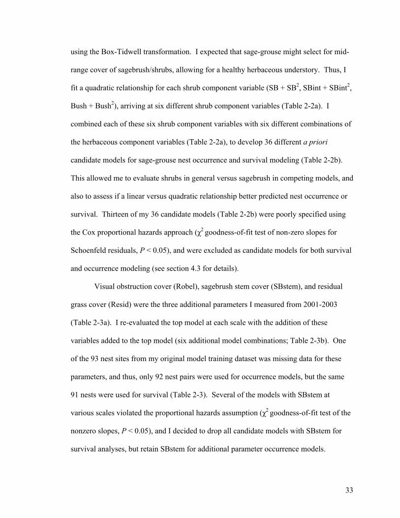
using the Box-Tidwell transformation. I expected that sage-grouse might select for mid-

range cover of sagebrush/shrubs, allowing for a healthy herbaceous understory. Thus, I

fit a quadratic relationship for each shrub component variable (SB + SB2, SBint + SBint2,

Bush + Bush2), arriving at six different shrub component variables (Table 2-2a). I

combined each of these six shrub component variables with six different combinations of

the herbaceous component variables (Table 2-2a), to develop 36 different a priori

candidate models for sage-grouse nest occurrence and survival modeling (Table 2-2b).

This allowed me to evaluate shrubs in general versus sagebrush in competing models, and

also to assess if a linear versus quadratic relationship better predicted nest occurrence or

survival. Thirteen of my 36 candidate models (Table 2-2b) were poorly specified using

the Cox proportional hazards approach (χ2 goodness-of-fit test of non-zero slopes for

Schoenfeld residuals, P < 0.05), and were excluded as candidate models for both survival

and occurrence modeling (see section 4.3 for details).

Visual obstruction cover (Robel), sagebrush stem cover (SBstem), and residual

grass cover (Resid) were the three additional parameters I measured from 2001-2003

(Table 2-3a). I re-evaluated the top model at each scale with the addition of these

variables added to the top model (six additional model combinations; Table 2-3b). One

of the 93 nest sites from my original model training dataset was missing data for these

parameters, and thus, only 92 nest pairs were used for occurrence models, but the same

91 nests were used for survival (Table 2-3). Several of the models with SBstem at

various scales violated the proportional hazards assumption (χ2 goodness-of-fit test of the

nonzero slopes, P < 0.05), and I decided to drop all candidate models with SBstem for

survival analyses, but retain SBstem for additional parameter occurrence models.

33

Residual grass (Resid) was highly correlated with grass cover (r > 0.77) at all scales, and

was not used in candidate models where the top 2001-2003 AICc-selected model at that

scale contained grass cover (Gr). This was the case only for all occurrence models (Table

2-3b). Thus, additional parameters added to occurrence models were Robel and SBstem,

and parameters added to survival models were Robel and Resid (Table 2-3b).

For all tables, due to their small values, I multiplied coefficients, standard errors,

and confidence intervals for the Bush2, SBint2, Gr, and GrHgt variables by 100 for

presentation purposes only. Forb is also multiplied by 100, but for occurrence models

only. I refer to non-multiplied values within the text.

4.2. Conditional fixed-effects occurrence analyses

Based on AICc weights (wi), top nest occurrence models did not have strong

support (i.e. wi > 0.90) at any of the scales tested for my original 2001-2003 training

dataset models (Tables 2-4 to 2-6), and only the nest-site scale showed strong selection

for the top additional parameter models (Tables 2-10 to 2-12). At all scales, however,

coefficient (βi) estimates were robust across all models, making inferences about those

parameters consistent, regardless of the model used. Thus, I chose not to model average

coefficients. Patterns in the coefficients were evident within the groups of top-selected

models, which I discuss for each scale.

4.2.1. Nest occurrence at the site scale

All 4 top candidate models at the nest-site scale contained the Bush + Bush2

parameters (Table 2-4). These four models were predictive, each explaining about 49%

of the variation in nest-site selection (Table 2-4). Inferences based on the coefficients

from the top model (#16) indicate sage-grouse select strongly for mid-to-high bush cover

34

above the nest (βBush = 0.156 ± 0.056, βBush2 = – 0.0007 ± 0.0009, concave function, Table

2-7). While there was no discernable selection for grass cover (Gr) at nest sites as the

95% CI confidence intervals overlapped zero (βGr = 0.0016 ± 0.0021, Table 2-7), there

was strong selection for grass that was considerably taller (βGrHgt = 0.048 ± 0.021, Table

2-7). The strength of influence of these parameters is evident from the relative variable

importance weightings where the Bush + Bush2 (∑wi = 0.99) and GrHgt (∑wi = 0.94)

terms had strong evidence of importance given my candidate set of models (Table 2-8).

Note that there was very weak evidence of importance for sagebrush (see all sagebrush

variables) unless sagebrush was combined with other shrubs in the Bush + Bush2 variable

(see Table 2-8 below dashed line).

This top AICc-selected nest site occurrence model (#16) had good fit (LR χ24 =

64.30, P < 0.001) and high model accuracy when predicted on both my training and

validation datasets (ROCtrain = 0.929, ROCtest = 0.930, Table 2-9). The model also had

excellent prediction (85%) for both training and testing datasets (Table 2-9).

The additional parameters model with both Robel and SBstem (model #16-5) was

the top AICc-selected model, had good fit (LR χ26 = 92.77, P < 0.001) and strong support

(wi = 0.90) within my candidate set of additional parameter models (Table 2-10).

Variance explained increased to 73% from the originally selected top AICc model (49%;

model #16; Table 2-10). Selection for mid-to-high amounts of bush cover above the nest

(βBush = 0.183 ± 0.083, βBush2 = – 0.0018 ± 0.0011) was still strong, and selection for taller

grass (βGrHgt = 0.044 ± 0.028) although weaker, was evident (Table 2-13). Strong

selection for greater obstruction cover (βRobel = 0.104 ± 0.046) and sagebrush stem cover

(βSBstem = 0.266 ± 0.091) explained the increase in deviance. These two variables

35

improved model accuracy when assessed on the training dataset (ROCtrain = 0.98) and

had excellent prediction (PCCtrain = 92.4%, Table 2-14).

4.2.2. Nest occurrence at the 7.5-m patch radius scale

There was weak support for the top AICc-selected model (#36) at the 7.5-m radius

scale (wi = 0.181, Table 2-5). All of the 8 models within the 90% confidence set (i.e. ∑wi

≥ 0.90), however, contained the SBint variable, and all but one model contained the

GrHgt variable (Table 2-5). All models at the 7.5-m radius scale explained >31% of the

variation in nest selection, with the top model (#36) explaining 37% of the variation

(Table 2-5). At this patch scale, based on the top model, sage-grouse appear to be more

selective for sagebrush as a canopy component than shrubs in general, but females are

selecting for mid-to-high range cover (βSBint = 0.792 ± 0.204, βSBint2 = – 0.028 ± 0.011,

concave function, Table 2-7). Selection was also strong for taller grass cover (βGrHgt =

0.078 ± 0.037), with females showing strong avoidance of other (non-palatable) forbs

(βForbOth = – 0.350 ± 0.172, Table 2-7). Ninety-five percent confidence intervals of βi

estimates for Gr and Forb overlapped zero, indicating neither selection nor avoidance

(Table 2-7). The strength of evidence for sagebrush cover estimated by the line intercept

method was strong (∑wi = 0.99) at this scale, with greater evidence for selection of

moderate sagebrush cover (i.e., quadratic relationship; SBint2 ∑wi = 0.64) over maximal

sagebrush cover (linear relationship; SBint ∑wi = 0.36, Table 2-8). This top AICc-

selected nest-occurrence model (#36) at the patch scale had good fit (LR χ26 = 48.26, P <

0.001), good accuracy (ROCtrain = 0.873, ROCtest = 0.884, Table 2-9), and good

prediction (PCCtrain = 78.5%, PCCtest = 82.5%, Table 2-9).

36

Of the additional parameters models, model #36-1 with the addition of Robel was

selected as the top AICc model and had good fit (LR χ27 = 54.70, P < 0.0001). There was

moderate support (wi = 0.72) for this model within my candidate set of additional

parameter models, and while the variance explained was better (42.9%), it only increased

6% over the base model (model 36; Table 2-11). Inferences about parameters with the

additional Robel variable were similar to the base model (see Table 2-7), with selection

remaining strong for mid-to-high ranges of sagebrush cover (Table 2-13). Taller grass

cover (βGr =0.060 ± 0.041), however, was now only weakly selected for and cover of

other forbs (βForbOth = – 0.321 ± 0.173) was only weakly avoided (Table 2-13). Even at

this patch scale (7.5 m from the nest), selection was again strong for greater obstruction

cover (βRobel = 0.127 ± 0.053, Table 2-13) and this model (#36-1) with Robel had high

model accuracy (ROCtrain = 0.89, Table 2-14) and good fit (PCCtrain = 80.4%; Table 2-

14), similar to the original base model (Table 2-9).

4.2.3. Nest occurrence at the 15-m radius scale

The top AICc-selected model (#25) at the 15-m radius area scale had very little

support, (wi = 0.173, Table 2-6). This model contained only the SBint and Gr variables,

and had similar weight to the second ranked model (#27; wi = 0.170, Table 2-6), which

only differed in structure by the addition of the GrHgt variable. Twelve models were

within the 90% confidence set (Table 2-6). Interestingly, 10 of those models contained

the SBint variable and 11 contained the Gr variable. Coefficient estimates were similar

across most top models and I chose to make inferences on the top AICc-selected model

(#25). Deviance explained for nest occurrence models at this area scale (between 16-

21% across top models) was less than at other scales (Table 2-6). Sage-grouse continued

37

to select for greater shrub (sagebrush at this scale) cover, even at this 15-m radius area

surrounding nest sites, as a positive increasing function, not a quadratic (βSBint = 0.398 ±

0.128, Table 2-7). Selection for greater grass cover also was evident, although weak (βGr

= 0.044 ± 0.023, Table 2-7). Again the strength of evidence for sagebrush cover

estimated by the intercept method was strong (∑wi = 0.84), and evidence weights also

suggest selection is linear (SBint ∑wi = 0.54), with sage-grouse selecting for the greatest

cover, compared to weak support for mid-range sagebrush cover at this area scale

(quadratic; SBint + SBint2 ∑wi = 0.30; Table 2-8). The top AICc-selected nest

occurrence model (#25) at the 15-m radius had good fit (LR χ23 = 16.25, P < 0.001), good

accuracy (ROCtrain = 0.775, ROCtest = 0.761), and prediction (PCCtrain = 71.0%, PCCtest =

75.0%) was reasonable (Table 2-9).

Of the models with additional parameters, model #25-3 with SBstem was the top

AICc model and had good fit (LR χ22 = 54.70, P < 0.0001). There was weak support (wi

= 0.351) within my candidate set of additional parameter models and the deviance

explained (18.51%) only improved marginally over the original model (15.82%, Table 2-

12). Again, the SBint and Gr coefficients were robust after the addition of the additional

SBstem variable (see Table 2-7) with strong selection still evident for greater sagebrush

cover but weak selection for greater grass cover (Table 2-13). Selection for SBstem was

moderate (βSBstem = 0.260 ± 0.148, Table 2-13), however, this model had good accuracy

(ROCtrain = 0.779) and reasonable prediction (PCCtrain = 72.43%, Table 2-14).

4.3. Proportional hazards survival analyses

Thirteen survival models were poorly specified using the Cox proportional

hazards approach (χ2 goodness-of-fit test of the nonzero slopes, P < 0.05) and these

38

models were dropped as candidate models for both survival and occurrence modeling

(see Table 2-2b). The same survival model (#22) was the top AICc-selected model at all

three scales tested, and was different from the top occurrence model at each scale (Table

2-15 to 2-17). In general, the fit, accuracy, prediction, and variation that could be

explained for nest survival models were lower than for occurrence models at all scales.

4.3.1. Survival at the nest site scale

The top AICc-selected nest site survival model (#22) had weak support (wi =

0.349), but similar to the occurrence models at this scale, all 6 top models within the 90%

confidence set contained the Bush + Bush2 variables (Table 2-15). Inferences based on

this model indicate that sage-grouse nests with mid-high range bush cover above the nest

(βBush= 0.954 ± 0.019, βBush2 = 1.000 ± 0.0003, convex function, Table 2-18) have a

reduced risk of failure. The risk of failure was also reduced with increasing forb cover

(βForb = 0.944 ± 0.030, moderate effect) and increasing grass height (βGrHgt = 0.997 ±

0.007, weak effect, Table 2-18). Similar to the occurrence models at the nest site, the

Bush + Bush2 term had strong evidence of importance (∑wi = 0.93), but Forb was also an

important variable (∑wi = 0.87, Table 2-19). Not surprisingly, all four models that

contained these variables (models 22, 18, 20, and 24, Table 2-15) explained the greatest

deviance (all ≈ 29% deviance explained). Finally, like the occurrence model at the nest

site, variable importance weightings suggest limited importance of sagebrush in

determining nest fate when not combined with other shrubs in the Bush + Bush2 variable

(∑wi = 0.93; Table 2-19).

This nest site survival model (#22) had good fit (LR χ24 = 19.50, P < 0.001), but

only moderate-to-good model accuracy (ROCtrain = 0.717, ROCtest = 0.727, Table 2-20).

39

Model prediction was lower for survival models (PCCtrain = 71.4%, PCCtest = 68.4%;

Table 2-20) compared to occurrence models at the nest-site scale. After classifying nests

within my training dataset as failed (1) or successful/censored (0) by predicting the top

model with the optimal cut-off point, I could easily differentiate nest survival to 28 days

between the two groups (Successful = 55.17 ± 8.4%, Failed = 17.9 ± 5.7%; Log-rank χ21

= 23.82, P < 0.0001). When this model was applied to my testing dataset, survival

differed greatly between the two groups (Successful = 51.3 ± 10.9%, Failed = 15.4 ±

10.0%), but due to similar survival functions over the first half of incubation, the Log-

rank test was weaker at detecting differences (χ21 = 23.82, P = 0.052).

The additional-parameters model with Resid (model #22-2) was the top AICc-

selected model. This model had good fit (LR χ25 = 23.14, P < 0.001) but weak support

(wi = 0.46) within my candidate set of additional parameter models (Table 2-21). Resid

only increased the deviance explained by 4% from the original model (Table 2-20).

Accuracy and prediction were not improved by the addition of Resid to the original nest-

site-survival model (ROCtrain = 0.719, PCCtrain = 69.2%; Table 2-20). Similar to the top

model without Resid, however, this additional parameter model still predicted well on the

training dataset, accurately differentiating survival for the censored nests (52.56 ± 8.48%)

from those that failed (20.20 ± 5.92%; Log-rank χ21 = 19.89, P < 0.0001). Surprisingly

though, as Resid increased at the nest site, risk of nest failure also increased (βResid =

1.027 ± 0.014), although only moderately so (CI range 1.001-1.054; Table 2-18).

Similarly, across most survival models tested containing the grass cover variable at the

nest-site scale, there was a trend for increased risk of nest failure with increasing grass

cover (βgrass > 1.0), but inferences were weak due to 95% CI that overlapped 1 for all

40

models. Figure 2-2 graphically shows these relationships between nest failure and each

parameter for model #22-2 at the nest site scale. Thresholds identified at the optimal cut-

off point predict nest survival with Bush >20 % cover, GrHgt >50 cm tall, Forb >6 %

cover, and Resid <2 % cover.

4.3.2. Survival at the 7.5-m patch scale

Twelve survival models at the patch scale were within the 90% confidence set

(Table 2-16). The top AICc-selected model (again model #22) had weak support (wi =

0.310), but explained slightly more deviance (32.75%; Table 2-16) than at the nest-site

scale (29% Table 2-16). Inferences about parameters were similar to those at the nest

site, but not as strong. The smaller Bush coefficient suggested a greater benefit with mid-

to-high range bush cover than at the nest site scale, (smaller βBush), the effect was not as

strong, with larger variance around those estimates (βBush = 0.935 ± 0.036, βBush2 = 1.001

± 0.001; convex function; Table 2-18). At this scale, however, greater forb cover (βForb =

0.937 ± 0.030) and taller grass (βGrHgt = 0.980 ± 0.001) both strongly reduced the risk of

nest failure; i.e., smaller coefficients with 95% CI that did not include 1 (Table 2-18).

There were no obvious trends in the parameters included within the top 12

models, but the variable importance weightings suggested that nest survival at the 7.5-m

scale was more strongly influenced by herbaceous understory than shrub canopy. Both

the GrHgt term (∑wi = 0.95) and the Forb term (∑wi = 0.84) had strong evidence of

importance, whereas the Bush and sagebrush terms all had moderate to weak evidence of

importance (all ∑wi ≤ 0.60; Table 2-19). This top 7.5-m, nest-survival model (#22) had

good fit (LR χ24 = 22.22, P < 0.001), low-to-good model accuracy (ROCtrain = 0.750,

ROCtest = 0.631, Table 2-20), but poorer prediction (PCCtrain = 65.9%, PCCtest = 55.3%,

41

Table 2-20). However, when predicting survival with this top model on both my training

(Survived = 52.0 ± 7.9%, Failed = 18.6 ± 6.3%) and testing datasets (Survived = 43.4 ±

9.1%, Failed = 0.0% - no nests hatched for this group), I could accurately differentiate

failed from successful nests (Training: Log-rank χ21 = 15.44, P < 0.0001; Testing: Log-

rank χ21 = 4.94, P = 0.026).

The addition of either Resid or Robel to nest-survival model #22 at the patch

scale resulted in slightly improved deviance estimates, but the penalty for additional

parameters resulted in the more parsimonious base model being selected (Table 2-22).

Of the additional-parameter models, the base model had only moderate support (wi =

0.516), primarily because model structure (parameters) changed little across candidate

models. Further inspection of coefficients across each model revealed the 95% CI

overlapped 1 for both Resid and Robel, suggesting limited importance of these

parameters at driving nest fate at the 7.5-m scale. Thus, I assessed the relationship

between nest failure and each parameter for model #22 at the 7.5-m patch scale (Figure 2-

3). Optimal cut-off points suggest thresholds at which nest survival is predicted for Bush

>5 % cover, GrHgt >17 cm tall, and Forb >3 % cover at the patch scale.

4.3.3. Survival at the 15-m area scale

Seven survival models at the 15-m area scale were within the 90% confidence set

(Table 2-17). The top AICc-selected model was again model #22, which also had weak

support (wi = 0.432) but good deviance explained (34.6%, Table 2-17). Variable

importance weights suggested the herbaceous understory (Forb ∑wi = 0.855, Grass ∑wi =

0.874) as well as the shrub layer (Bush + Bush2 ∑wi = 0.830) were important in

predicting nest survival at this large-area scale, with the importance of sagebrush

42

enhanced when combined with all shrubs (i.e., Bush terms; Table 2-19). Inferences about

this model were similar to other scales (LR χ24 = 22.22, P < 0.001), with risk of failure

reduced with moderate-to-high bush cover (βBush= 0.918 ± 0.044, βBush2 = 1.000 ± 0.002),

greater forb cover (βForb = 0.956 ± 0.025), and taller grass (βGrHgt = 0.979 ± 0.011, Table

2-18). However, all effects were weak (95% CI just overlap 1; Table 2-18). With only

good-to-poor model accuracy (ROCtrain = 0.766, ROCtest = 0.531) and poor prediction

(PCCtrain = 69.3%, PCCtest = 55.3%) my models were weakest at capturing mechanisms of

nest failure at the 15-m scale. I could predict survival accurately using this top model

and cut-point for my training dataset (Survived = 52.3 ± 8.2%, Failed = 17.0 ± 6.0%;

Log-rank χ21 = 14.47, P = 0.0001), but I had poor predictive ability when applied to the

testing dataset (Survived = 40.7 ± 11.8%, Failed = 37.0 ± 11.9%; Log-rank χ21 = 0.29, P

= 0.587).

Additional parameters Resid and Robel resulted in minor improvements in

deviance explained (Table 2-23), but similar to the patch scale, the base model #22 was

selected as the top AICc model again, with only weak support (wi = 0.342; Table 2-23).

All models containing the additional parameters Resid and Robel added little power to

explain nest survival at the 15 m area scale (95 % CI overlapped 1 in all cases). Thus,

similar to the patch scale, I used model #22 to graphically show the relationship between

nest failure and each parameter at the 15 m nest area scale. Optimal cut-off points

suggest thresholds at which nest survival is predicted for Bush >7 % cover, GrHgt >27

cm tall, and Forb >7 % cover at the 15 m area scale.

43

5. Discussion

My models were excellent at predicting sage-grouse nest selection (occurrence) in

southern Alberta. Even when predicted on an independent sample of data, the models

validated well, with high prediction and classification accuracy (Table 2-9). With the

additional parameters in the top models, I could explain as much as 73% of the variation

in nest occurrence (Table 2-14). The best predictions were at the nest-site scale.

Hierarchical habitat selection by sage-grouse for nest sites is evident, with different

parameters selected at different scales; the area, the patch, and the nest-site scales. As

expected, sage-grouse selected for nest habitats that provide structural cover from shrubs

(sagebrush and other shrubs) as well as from herbaceous understory vegetation that

concealed the nest. Selection is strong for a large area (15-m radius scale) of thick

sagebrush cover which contains greater amounts of grass (moderate selection, Table 7).

Within this area, females again selected strongly for a patch (7.5-m radius scale) of dense

sagebrush (quadratic function), although the densest patches are avoided. Patches

containing taller grass (Table 2-7) and greater visual obstruction cover were selected

(Table 2-13). Finally, within this patch, females chose to place their nest under

sagebrush, but appear to shift their focus to include cover provided by additional shrubs

immediately surrounding the nest site (Tables 2-7, 2-13), again avoiding the densest

canopies. Wiebe and Martin (1998) found that white-tailed ptarmigan (Lagopus

leucurus) also selected for intermediate cover at the nest site. They suggest that females

are making a trade-off that allows for a better view of predators within the nest

surrounding (Wiebe and Martin 1998). Sage-grouse also may be recognizing these

44

ecological cues similarly, selecting for intermediate-to-high shrub cover, because nest

failure was reduced for those selecting moderate ranges of cover.

Within the patch scale, taller grass cover still is selected strongly at the nest site

(Table 2-7), along with enhanced visual obstruction cover and additional nest

concealment provided by woody sagebrush stem (Table 2-13). Habitat with high

obstruction or concealment cover has been shown to be important for nesting for several

other grouse species (Lutz et al. 1994; Wiebe and Martin 1998; Manzer 2004) as well as

sage-grouse (Gregg et al. 1994), and survival can be enhanced with increased

concealment cover (Lutz et al. 1994; Manzer 2004).

Variable importance weightings are useful for making generalizations about the

relative importance of variables within a candidate set of models. Weights for variables

from occurrence models also suggest that hierarchical selection is taking place. For

example, weights highlight the importance of dense sagebrush cover in the area

surrounding a nest, and the importance of moderate cover of sagebrush patches within

that area. The overwhelming importance of moderate-to-high range cover of additional

shrubs at the nest site was also evident from the variable importance weights (Table 2-8).

Grass height was an important variable at all scales tested, increasing in importance

closer to the nest site (Table 2-8). Together, these importance weights reinforce the

significance of both shrub-canopy cover and herbaceous-obstruction cover selected by

female sage-grouse for nesting. A tall shrub canopy is necessary to conceal nests from

avian predators, and tall herbaceous understory also is necessary, possibly acting as a

visual barrier obscuring nests (Martin 1993; Crawford et al. 2004) from terrestrial

predators.

45

When using variable importance weights, Burnham and Anderson (2002: 169)

suggest ensuring “a balance in the number of models that contain each variable” so as to

“put each variable on equal footing.” Although I had high variability in the number of

candidate models for which each variable occurred, I chose to identify biologically

meaningful models a priori, rather than ‘cook’ my candidate set to have even variable

occurrence across all models. This may influence the relative variable importance, but in

many cases, I saw variables that occurred in few models, such as the Bush + Bush2

variable (in 6 of 23 occurrence models at the nest site scale) have the greatest variable

importance (∑wi ≥ 0.99, Table 2-8), and variables such as Forb that were in over twice as

many models (in 13 of 23 occurrence models at the area scale), have relatively low

variable importance (∑wi ≥ 0.27; Table 2-8). Thus, I feel that the importance weights are

valid relative measures of the strength of variable importance in my models, and also add

support to my decision to make inferences using the top AICc-selected model within each

candidate set.

Hierarchical selection of habitat by wildlife species is not a new concept (Meyer

et al. 1998; Breininger et al. 1998; Johnson et al. 2001; Boyce et al. 2003; Mcgrath et al.

2003), although often only a single scale of selection is addressed. Although Aldridge

and Brigham (2002) have addressed hierarchical selection by sage-grouse with selection

at multiple scales for sagebrush, my models incorporating more complex designs

illustrate detailed and differing selection patterns across these hierarchical scales. My

results suggest that nesting habitat requirements are not uniform surrounding a nest site,

nor across a landscape. Management focused on nest site characteristics alone, which has

been the focus of many nesting habitat studies for prairie grouse (Gregg et al. 1994; Lutz

46

et al. 1994; Sveum et al. 1998b), could lead to sub-optimal habitat provisioning for the

species of interest.

Sage-grouse nest success varies widely across the species range (15-86%) but is

typically between 30-60% (see Schroeder et al. 1999). Nest survival in my study (35.3 ±

5.37%) was at the low end of this range, and slightly lower than previous research in

Alberta from 1998-1999 (46%, n = 29, Aldridge and Brigham 2001). However, as

Aldridge and Brigham (2001) suggest, above normal spring precipitation, which has been

positively correlated with nest success (Gill 1966), may result in elevated nest success.

My study spanned the final 2 years (2000-2001) of an extreme 3-year drought period in

southern Alberta, possibly resulting in slightly lower nest success. However, I did not

detect differences in nest success between grouped years for my training (2001-2003) and

testing (1998-2000) datasets (Log-rank χ21 = 0.27, P = 0.61).

Given that females are highly selective, it is not surprising that the predictive

capabilities for my nest survival models were lower, particularly for the independent

(1998-2000) nest validation sample. I believe that this may also be a sample size issue,

having only 40 nests with 22 failures in my validation dataset. Survival analyses with

<25 samples per treatment group rarely provide adequate results, and in most cases, 50

samples per group are required (Pollock et al. 1989; Winterstein et al. 2001). As is the

case for most wildlife telemetry studies, particularly when data are limited for

endangered species, one can not often afford to partition samples into model training and

testing datasets. Even though nest success was greater in prior years (testing dataset) and

my testing dataset sample size was small, I was still able to differentiate failed from

successful nests at most scales.

47

Occurrence models indicated females select for mid-high shrub cover (Bush

variable) at the nest site only. However, survival models at all scales (model #22)

suggest that females who select for shrub cover at the nest site as well as the larger patch

and area scales surrounding the nest are more likely to be successful. The Bush

parameter was largely composed of sagebrush, with other shrubs adding between 2-6%

additional canopy cover (Table 2-1). Thus, selection for only sagebrush may result in

similar nest success. This was not the case however, and importance weights over all

survival models indicate that the Bush + Bush2 played a greater role in nest survival than

sagebrush alone, or using the combined weights for all sagebrush variables (Table 2-19).

Other research has shown that sage-grouse tend to select more dense sagebrush to place

their nests under, and nests with greater canopy cover are more successful (Klebenow

1969; Wallestad and Pyrah 1974; Connelly et al. 1991; Gregg et al. 1994; Sveum et al.

1998b; Aldridge and Brigham 2002). However, in Alberta, cover from sagebrush is

limited (5-10%, my study and Aldridge and Brigham 2002) compared to that in other

areas (Schroeder et al. 1999; Connelly et al. 2004). Thus, females may recognize the

general importance of canopy structure and select for additional cover provided by other

shrubs, at least at the nest site itself. Beyond the nest site, additional shrub cover also

reduces the risk of failure, but females are not as efficient at recognizing cues at these

scales as shrubs were not selected for in the occurrence models, possibly creating

ecological traps (Delibes et al. 2001; Donovan and Thompson 2001). Bock and Jones

(2004) found a negative relationship between population density and reproductive

success for many bird species when present in human-disturbed habitats. They suggested

that birds fail to recognize these ecological traps when the human-altered landscape

48

differed from that in which the birds evolved. Sage-grouse appeared to focus on

sagebrush as the most important component of nesting habitat, but reductions in

sagebrush availability, possibly from human-related causes (discussed below), may have

increased the importance of other shrubs; a benefit sage-grouse fail to recognize beyond

the nest site itself.

Residual grass was correlated with total grass cover, preventing the addition of

Resid to the additional parameters occurrence models. However, females did not show

selection or avoidance of residual grass cover at any scale in univariate models (see Table

2-1 for means). Although I expected residual grass cover to be greater at successful

nests, this was not the case. Survival at the nest-site scale (i.e., within 0.5 m of the nest)

was reduced with increasing residual grass cover (Successful = 9.2 ± 1.6%; Failed = 4.9 ±

1.0%; Figure 2-3). This relationship did not exist at other scales; at the patch and area

scales, 95% CI for βResid for model #22-2 overlapped 1. McKee et al. (1998) found that

excessive litter (>25%), defined as horizontally oriented vegetation from the previous

year, resulted in reduced nest success for greater prairie-chickens (Tympanuchus cupido

pinnatus) in Missouri. Although I do not believe that there was an excessive build up of

residual plant material during my study (8% residual grass cover, Table 2-3), it has been

suggested that new plant growth, and thus height of nest cover vegetation, may be

delayed by a build up of matted dead matter (Westemeier 1973; Mckee et al. 1998).

However, this is not likely to occur in the xeric dry mixedgrass ecosystem of southern

Alberta. Although grass height and residual grass cover were not correlated (rs ≤ 0.16, n

= 186, for all three scales), it is possible that reduced residual-grass cover at successful

49

nest sites is a result of selection for taller herbaceous vegetation, which reduces the risk

of nest failure.

Despite exhibiting strong selection of tall grass for nest concealment at all scales,

grass height was still an important contributor to nest survival at all scales. Conversely,

although females did not select for forbs at any scale, nest success increased for those that

selected greater forb cover; a trend detected across all scales. This reinforces the

importance of surrounding tall herbaceous understory vegetation or lateral cover for

successful nesting (Wallestad and Pyrah 1974; Gregg et al. 1994; Sveum et al. 1998b;

Aldridge and Brigham 2002; Watters et al. 2002), and may reflect larger patch-level

ecological cues that are not being recognized by sage-grouse. In addition, given that

forbs could enhance nest success, and the diet for precocial sage-grouse chicks

immediately after they hatch (Johnson and Boyce 1990; Sveum et al. 1998a; Aldridge

and Brigham 2002), it is surprising that females do not recognize these benefits and

choose to nest in areas with greater forb cover.

Variable importance weights suggested forbs (palatable to sage-grouse)

contributed strongly to survival models at all three scales (Table 2-19). Grass height had

strong evidence of support at the patch and area scales, and moderate importance at the

nest site, again supporting the importance of herbaceous understory vegetation

(Wallestad and Pyrah 1974; Gregg et al. 1994; Sveum et al. 1998b; Aldridge and

Brigham 2002; Watters et al. 2002). There was strong variable importance for the Bush

+ Bush2 parameter (moderate-high cover) at both the nest site and the 15-m area scale,

but only moderate importance at the 7.5-m patch scale. There was additional evidence in

50

support of the importance of sagebrush (SBint parameter) for the patch-scale survival

models, although it was weak (Table 2-19).

Based on the variable importance weights for both occurrence and survival

models, the line intercept technique (Canfield 1941) is a better approach for measuring

sagebrush canopy cover (to correlate with sage-grouse nest site selection and nest

success) than using 1-m2 quadrats. Although these two methods are correlated, and as

Daubenmire (1959) pointed out, too few quadrats may result in highly variable and

possibly overestimated canopy measures for shrubs. Both measures produced similar

mean cover estimates (Table 2-1) in my study, but future research conducted on

sagebrush-steppe habitats should use the line intercept method to assess sagebrush (and

shrub) canopy coverage, as recommended by the sage-grouse management (Connelly et

al. 2000) and monitoring (Connelly et al. 2003) guidelines.

Even though most nests (81%) were at least partially located under sagebrush,

many were covered or surrounded by other shrubs such as snowberry (Symphoricarpos

albus), rose (Rosa spp.), greasewood (Sarcobatus vermiculatus), wolf willow (Elaeagnus

commutata), and occasionally creeping juniper (Juniperus horizontalis). Not surprisingly

then, nest fate was directly affected by other shrubs (Bush + Bush2 parameters), and this

relationship existed at all three scales measured (nest site, 7.5-m patch scale, and 15-m

area scale). Thus, sage-grouse are only partially recognizing ecological cues linked to

fitness. Other studies have shown that nest survival is unrelated to the shrub species the

nest is placed under (Sveum et al. 1998b; Aldridge and Brigham 2003) while others still

have shown that success is reduced when nests are not placed under sagebrush (Connelly

et al. 1991). I show that nest success could actually be enhanced when shrubs, in

51

addition to sagebrush, are selected. Given that sagebrush is not abundant within the

Alberta range of sage-grouse (~2% cover at random areas and 12-14% cover at the

random sites; Table 2-1) compared other areas throughout the range (15-25%; Schroeder

et al 1999; Connelly et al. 2000), sage-grouse may be selecting for additional cover from

other shrubs. As Aldridge and Brigham (2003) pointed out, as long as suitable shrub

cover is available, the species providing it might not matter.

My predictive models allow me to make inferences and identify threshold levels

for parameters in my models. Given that the same survival model (#22) with the same

parameters was selected at all three scales, pasture-level management providing

vegetation that meets or exceeds these model thresholds will increase nest success for

sage-grouse. Although trends were similar at all scales, I discuss in detail here

predictions and thresholds based on the 7.5-m radius scale for three reasons. Firstly,

management of shrubs and herbaceous understory does not take place at the scale of a

single sagebrush plant and the vegetation within a 1-m2 quadrat surrounding it.

Management takes place at the scale of a large habitat patch, or pasture, thus, I felt that

the patch or area scale (7.5 m or 15 m) would be more appropriate. Secondly, my models

indicate that selection is taking place beyond the nest site itself, and that nest fate can be

affected by vegetation at these greater patch and area scales. Finally, my survival model

at the patch scale was more accurate and had better predictive capacity than the 15-m

area scale model. Given that the relationship between nest survival and each parameter is

similar for all scales, when managing habitat for conservation purposes, I recommend the

more conservative (i.e. greater cover or height threshold) be used. Several management

options may exist that could achieve these desired goals (i.e., various grazing strategies,

52

active management of sagebrush, etc.), but I recommend these approaches be tested

within the experimental framework of an adaptive management process (Chapter 5,

Aldridge et al. 2004).

Small increases in sagebrush cover on the landscape (i.e., 5-10%) might be

enough to elevate productivity to stabilize productivity in the Alberta sage-grouse

population (Aldridge and Brigham 2002). Using βi coefficients, presented here as

exponentiated estimates or risk of nest failure for a single unit increase in a particular

parameter, I can assess the risk of failure for varying availabilities of the parameter of

interest. For the patch survival model (#22), the combined estimates for βBush and βBush2

(Table 2-18) indicates the risk of nest failure (βBush+ βBush2 = 0.9353) decreases by about

7% for each 1% increase in bush cover; although this relationship is not linear. Thus, if

bush cover was increased by 5%, nest failure (βBush+ βBush2 =0.7248) would be reduced by

about 27%. A 10% increase (βBush+ βBush2 =0.5398) will cut nest failure rates by about

half. An increase of sagebrush cover (the primary component of Bush) by 5-10%, would

provide enhanced breeding habitat for sage-grouse, providing 15-20% cover in Alberta,

and double the chance of nests successfully hatching. This can be seen graphically in

Figure 2-3a, where I assess the relative nest failure hazard by varying the bush parameter

while keeping all other parameters at their mean values. An increase in bush cover from

that currently available (~5%, Table 2-1) to >10%, would result in the majority of habitat

falling below the optimal cut-point, and drastically reduce the risk of nest failure (Figure

2-3a). Similarly, at >15% bush cover, there is little change in the risk of nest failure,

suggesting a potential management target where the greatest increase in nest success per

unit increase in sagebrush will be achieved. These thresholds strongly support suggested

53

the minimum management target of 15% sagebrush cover for sage-grouse breeding

habitat (Connelly et al. 2000).

Although sagebrush stem was selected at both the nest site and the 15-m area

scales, I was unable to test the effect of stem on nest survival due to the SBstem

parameter violating the proportional hazards assumption. I hypothesize however, that

selection for sagebrush stem, and the Bush parameter (combined sagebrush + other

shrubs) is likely a consequence of females recognizing the importance of structural cover,

and selecting for it regardless of the type. This also might suggest a lack of suitable

sagebrush cover on the landscape. A. cana is one of the few fire-successional Artemisia

species that resprouts vegetatively after spring fires (Tisdale and Hironaka 1981;

Wambolt et al. 1990; Adams et al. 2004). Reduced fire frequencies associated with fire

suppression on the Canadian prairies (Adams et al. 2004) may result in decreased

sagebrush abundance, rendering plants older and more decadent. Recent drought

conditions have reduced the number of episodic flood events, which can also enhance the

resprouting of A. cana. (Adams et al. 2004). Combined, the reduced abundance of

vigorous and mature, but not decadent sagebrush, could potentially limit high-quality

habitats required to maintain viable populations of sage-grouse, as well as other

sagebrush obligates on the dry mixedgrass prairie. This relationship needs to be explored

further.

Ideally, to truly represent habitat quality through assessing fitness, one must

include measures of both survival and reproduction. Here, I have used one measure of

reproduction (nest survival) as a surrogate for fitness. As Franklin et al. (2000) illustrate

for spotted owls, habitat variation can affect components of fitness very differently.

54

Thus, while my nest models may not capture fully all processes linked to fitness (i.e.,

brood survival and habitat use, and female survival and habitat use across different

seasons), and I did not directly assess any measures associated with human use, I feel that

these models are an important initial step that provide managers with the tools necessary

to provide high-quality nesting habitats for sage-grouse in Alberta, and ensure females

are likely to use those habitat and be successful in doing so.

6. Conclusions

Based on my nest occurrence and survival models, management for sage-grouse

nesting habitats in southern Alberta should be aimed at providing 1) suitable abundance

of healthy sagebrush cover, and 2) suitable cover and height of herbaceous understory

vegetation. Given the low availability of sagebrush in Alberta, females are selecting for

sagebrush (patch and area scales) and additional shrub cover (nest site scale) at nests.

Nest success is driven strongly by shrub cover and could be improved with slight

increases in sagebrush abundance. The ecology of silver sagebrush is poorly understood

(Adams et al. 2004), and potential management actions following an adaptive

management approach (Aldridge et al. 2004) would be beneficial to increase knowledge

and means to improve range health in sagebrush habitats. In doing so, one must continue

to monitor how sage-grouse respond to management actions. Initial management goals

should be aimed at maintaining or enhancing sagebrush, resulting in large areas with

overall cover of 10-20% (Figures 2-3, 2-4). Within these areas, heterogeneous patches

should exist, some with 30 to 40% cover, which will increase the chance of birds using

these habitats and also enhance nest success.

55

The importance of herbaceous understory vegetation in providing high-quality

sage-grouse nesting habitat has been recognized by others (Gregg et al. 1994; Sveum et

al. 1998b; Connelly et al. 2004; Crawford et al. 2004). I provide models identifying

understory vegetation thresholds at multiple scales that must be maintained if areas are to

be selected, and successfully used for nesting by females, ensuring productive

populations. Thresholds suggest that managers should strive to maintain grass within

sagebrush habitats that is 18-30 cm in height with a healthy forb component of at least

6% forb cover; greater cover of forbs (10-15%) will increase the likelihood of nest

survival. Within those areas, ensuring some patches have sites with even taller grass

(>50 cm) to provide additional structural cover necessary to conceal nests will further

reduce the risk of nest failure. My results suggest that mid-seral range conditions may be

of greater value than more traditional manament for late-seal or more climax

communities.

Even though inferences from prior research identify cursory nesting habitat

requirements for sage-grouse in Alberta, and go so far as to suggest that sagebrush may

be limiting (Aldridge and Brigham 2002), management efforts have yet to result in any

on-the-ground initiatives to enhance habitat for this endangered population. While

numbers continue to decline, managing for high quality habitat to ensure productive

populations is increasingly important, especially given the devastating consequences that

stochastic events such as West Nile virus pose (Naugle et al. 2004). My threshold

models provide managers with the tools necessary to begin implementing practices to

enhance sage-grouse habitats in Alberta. I hope that these tools will be used to identify

56

and maintain critical (nesting) habitat for sage-grouse, as required by the Federal Species

at Risk Act (SARA).

57

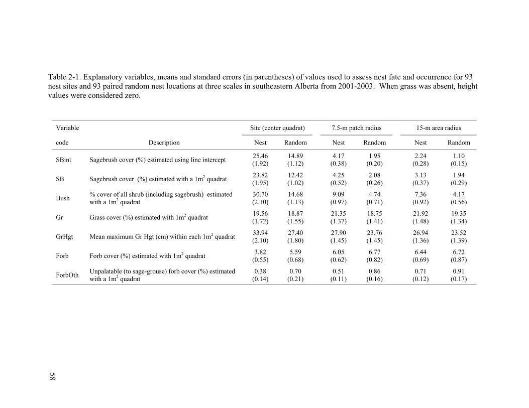
Table 2-1. Explanatory variables, means and standard errors (in parentheses) of values used to assess nest fate and occurrence for 93 nest sites and 93 paired random nest locations at three scales in southeastern Alberta from 2001-2003. When grass was absent, height values were considered zero.

Variable Site (center quadrat) 7.5-m patch radius 15-m area radius

code Description Nest Random Nest Random Nest Random

SBint Sagebrush cover (%) estimated using line intercept 25.46 (1.92)

14.89 (1.12)

4.17 (0.38)

1.95 (0.20)

2.24 (0.28)

1.10 (0.15)

SB Sagebrush cover (%) estimated with a 1m2 quadrat 23.82 (1.95)

12.42 (1.02)

4.25 (0.52)

2.08 (0.26)

3.13 (0.37)

1.94 (0.29)

Bush % cover of all shrub (including sagebrush) estimated with a 1m2 quadrat

30.70 (2.10)

14.68 (1.13)

9.09 (0.97)

4.74 (0.71)

7.36 (0.92)

4.17 (0.56)

Gr Grass cover (%) estimated with 1m2 quadrat 19.56 (1.72)

18.87 (1.55)

21.35 (1.37)

18.75 (1.41)

21.92 (1.48)

19.35 (1.34)

GrHgt Mean maximum Gr Hgt (cm) within each 1m2 quadrat 33.94 (2.10)

27.40 (1.80)

27.90 (1.45)

23.76 (1.45)

26.94 (1.36)

23.52 (1.39)

Forb Forb cover (%) estimated with 1m2 quadrat 3.82 (0.55)

5.59 (0.68)

6.05 (0.62)

6.77 (0.82)

6.44 (0.69)

6.72 (0.87)

ForbOth Unpalatable (to sage-grouse) forb cover (%) estimated with a 1m2 quadrat

0.38 (0.14)

0.70 (0.21)

0.51 (0.11)

0.86 (0.16)

0.71 (0.12)

0.91 (0.17)

58

Table 2-2. Shrub and herbaceous component models used to generate a prior candidate models are shown in (a) for nest site occurrence modeling and survival based on 93 nest sites and 93 paired random nest locations in southeastern Alberta from 2001-2003. Each of the six shrub component models were combined with each of the six herbaceous component models, for a total of 36 different initial candidate models (b). Thirteen models marked asterisk (*) were removed due to violations of the proportional hazards assumption for survival models, leaving 23 candidate models for survival and occurrence modeling. a)

Shrub Component Variables Herbaceous Component Variables

SB GrSB + SB2 Gr + GrHgt Bush Gr + Forb Bush + Bush2 Gr + GrHgt + Forb SBint Forb + GrHgt SBint + SBint2 Gr + GrHgt + Forb + ForbOth

b)

# Structure for Sagebrush Quadrat Models # Structure for Bush Models # Structure for Sagebrush Intercept Models

1- SB + Gr *13- Bush + Gr 25- SBint + Gr

2- SB + SB2 + Gr 14- Bush + Bush2 + Gr 26- SBint + SBint2 + Gr

3- SB + Gr + GrHgt *15- Bush + Gr + GrHgt 27- SBint + Gr + GrHgt

4- SB + SB2 + Gr + GrHgt 16- Bush + Bush2 + Gr + GrHgt 28- SBint + SBint2 + Gr + GrHgt

*5- SB + Gr + Forb *17- Bush + Gr + Forb *29- SBint + Gr + Forb

*6- SB + SB2 + Gr + Forb 18- Bush + Bush2 + Gr + Forb *30- SBint + SBint2 + Gr + Forb

7- SB + Gr + GrHgt + Forb *19- Bush + Gr + GrHgt + Forb 31- SBint + Gr + GrHgt + Forb

8- SB + SB2 + Gr + GrHgt + Forb 20- Bush + Bush2 + Gr + GrHgt + Forb 32- SBint + SBint2 + Gr + GrHgt + Forb

*9- SB + Forb + GrHgt *21- Bush + Forb + GrHgt 33- SBint + Forb + GrHgt

*10- SB + SB2 + Forb + GrHgt 22- Bush + Bush2 + Forb + GrHgt 34- SBint + SBint2 + Forb + GrHgt

11- SB + Gr + GrHgt + Forb + ForbOth *23- Bush + Gr + GrHgt + Forb + ForbOth 35- SBint + Gr + GrHgt + Forb + ForbOth

*12- SB + SB2 + Gr + GrHgt + Forb + ForbOth 24- Bush + Bush2 + Gr + GrHgt + Forb + ForbOth 36- SBint + SBint2 + Gr + GrHgt + Forb + ForbOth

59

Table 2-3. The additional explanatory parameters, means, standard errors (in parentheses) and range of values used to assess nest occurrence for 92 nest sites and 92 paired random nest locations at all three scales in southeastern Alberta from 2001-2003 are shown in a). Observations were not recorded for one nest pair which was dropped. The model structure of additional parameters added to the top AICc-selected model at each scale is shown in b). Note: All models with SBstem violated the proportional hazards assumption, and thus those models were dropped only as candidate survival models. Residual grass (Resid) was highly correlated with grass cover (r >0.70) and was not used in candidate models where the top 2001-2003 AICc-selected model at that scale contained Gr (this was the case for all occurrence models only). a)

Variable Site (center quadrat) 7.5-m patch radius 15-m area radius code Description Nest Random Nest Random Nest Random

Robel Visual obstruction reading (height in cm) measured at 2m from pole

26.33 (1.37)

13.14 (0.84)

8.43 (0.80)

5.43 (0.55)

6.53 (0.56)

5.08 (0.45)

SBstem Cover (%) provided from sagebrush stem using a 1m2 quadrat

14.40 (1.41)

5.63 (0.77)

2.09 (0.35)

0.86 (0.21)

1.02 (0.15)

0.58 (0.12)

Resid Residual grass cover (%) estimated using a 1m2 quadrat

7.76 (1.11)

8.37 (1.12)

8.61 (0.93)

8.01 (0.96)

8.93 (1.02)

8.06 (0.90)

b)Model # Structure for 2001-2003 additional parameters models

Top # (Top AICc-selected model for any given scale)

Top #-1 (Top model ) + Robel

Top #-2 (Top model ) + Resid

Top #-3 (Top model ) + SBstem

Top #-4 (Top model ) + Robel + Resid

Top #-5 (Top model ) + Robel + SBstem

Top #-6 (Top model ) + Resid + SBstem

Top #-7 (Top model ) + Robel + Resid + SBstem

60

Table 2-4. AICc-selected nest occurrence models, Akaike weights (wi) for all models comprising a cumulative AICc weight (∑wi) of ≥ 0.90 at the nest site (center quadrat). All model Likelihood Ratio (LR) χ2 tests were significant at P < 0.001. Percent deviance (Dev.) explained indicates the reduction in the log-likelihood from the null model. Model

# Model Structure Log-Likelihood K AICc ∆i AICc wi ∑ wi

Model LR χ2

% Dev. Explained

16 Bush + Bush2 + Gr + GrHgt – 32.313 4 73.081 0.000 0.426 0.426 64.30 49.87

22 Bush + Bush2 + Forb + GrHgt – 32.589 4 73.633 0.552 0.324 0.750 63.75 49.44

20 Bush + Bush2 + Gr + GrHgt + Forb – 32.303 5 75.295 2.215 0.141 0.891 64.32 49.89

14 Bush + Bush2 + Gr – 35.599 3 77.467 4.387 0.048 0.938 57.73 44.78

61

Table 2-5. AICc-selected nest occurrence models, Akaike weights (wi) for all models comprising a cumulative AICc weight (∑wi) of ≥ 0.90 for the 7.5-m radius scale from the nest site. All model Likelihood Ratio (LR) χ2 tests were significant at P < 0.001. Percent deviance (Dev.) explained indicates the reduction in the log-likelihood from the null model.

Model


Model LR χ2

% Dev. Explained

36 SBint + SBint2 + Gr + GrHght + Forb + ForbOth – 40.334 6 93.645 0.000 0.181 0.181 48.26 37.43

28 SBint + SBint2 + Gr + GrHgt – 42.713 4 93.880 0.236 0.160 0.341 43.50 33.74

34 SBint + SBint2 + Forb + GrHgt – 42.725 4 93.905 0.261 0.159 0.500 43.47 33.72

27 SBint + Gr + GrHgt – 44.328 3 94.925 1.280 0.095 0.595 40.27 31.24

33 SBint + Forb + GrHgt – 44.328 3 94.926 1.281 0.095 0.690 40.27 31.23

26 SBint + SBint2 + Gr – 44.429 3 95.128 1.484 0.086 0.776 40.07 31.08

35 SBint + Gr + GrHgt + Forb + ForbOth – 42.224 5 95.138 1.494 0.086 0.861 44.48 34.50

32 SBint + SBint2 + Gr + GrHgt + Forb – 42.707 5 96.104 2.460 0.053 0.914 43.51 33.75

62

Table 2-6. AICc-selected nest occurrence models, Akaike weights (wi) for all models comprising a cumulative summed AICc weight (∑wi) of ≥ 0.90 for the 15-m radius scale from the nest site. All model Likelihood Ratio (LR) χ2 tests were significant at P < 0.001. Percent deviance (Dev.) explained indicates the reduction in the log-likelihood from the null model.

Model


Model LR χ2

% Dev. Explained

25 SBint + Gr 53.986 2 112.105 0.000 0.173 0.173 20.95 16.25

27 SBint + Gr + GrHgt 52.934 3 112.138 0.033 0.170 0.342 23.06 17.88

26 SBint + SBint2 + Gr 53.511 3 113.292 1.187 0.095 0.438 21.90 16.99

28 SBint + SBint2 + Gr + GrHgt 52.472 4 113.398 1.293 0.090 0.528 23.98 18.60

33 SBint + Forb + GrHgt 53.599 3 113.469 1.364 0.087 0.615 21.73 16.85

31 SBint + Gr + GrHgt + Forb 52.889 4 114.232 2.128 0.060 0.675 23.15 17.95

14 Bush + Bush2 + Gr 53.986 3 114.242 2.137 0.059 0.734 20.95 16.25

35 SBint + Gr + GrHgt + Forb + ForbOth 51.953 5 114.596 2.491 0.050 0.784 25.02 19.41

34 SBint + SBint2 + Forb + GrHgt 53.092 4 114.638 2.533 0.049 0.832 22.74 17.64

36 SBint + SBint2 + Gr + GrHgt + Forb + ForbOth 51.211 6 115.400 3.295 0.033 0.866 26.50 20.56

32 SBint + SBint2 + Gr + GrHght + Forb 52.381 5 115.452 3.347 0.032 0.898 24.16 18.74

16 Bush + Bush2 + Gr + GrHgt 53.702 4 115.858 3.753 0.026 0.924 21.52 16.69

63

Table 2-7. Estimated coefficients (βi), standard errors (shown in parentheses), and 95% confidence intervals for top AICc-selected candidate nest occurrence models in south-eastern Alberta for all scales. Models were developed on 93 nest sites and 93 paired random locations collected from 2001-2003.

Confidence intervals Confidence

intervals Confidence intervals

Variable Nest Site Model 16

Lower

Upper

7.5-m radius Model 36

Lower

Upper

15-m radius Model 25

Lower

Upper

Bush 0.156 (0.056) 0.046 0.266

aBush2 – 0.069 (0.089) – 0.243 0.106

SBint 0.792 (0.204) 0.392 1.192 0.398

(0.128) 0.147 0.649

aSBint2 – 2.807 (1.068) – 4.900 – 0.714

aGr 1.573 (2.121) – 2.584 5.731 – 2.074

(2.686) – 7.339 3.192 4.044 (2.348) – 0.558 8.645

aGrHgt 4.805 (2.063) 0.761 8.848 7.779

(3.716) 0.497 15.062

aForb – 1.766 (5.589) – 12.72 9.189

ForbOth – 0.350 (0.172) – 0.687 – 0.014

aCoefficients, standard errors, and confidence intervals for Bush2, SBint2, Gr, GrHgt and Forb have been multiplied by 100.

64

Table 2-8. Relative variable importance for nest occurrence models (2001-2003), based on the sum of the AICc weights for each variable across all models. (n=93 nest sites and 93 paired random locations). Sagebrush variables below the double line illustrate the strength of the measurement technique (quadrats vs. line intercept) and the importance of the quadratic relationship at each scale. Parameter Model Freq. indicates the frequency for each parameter occurring across all 23 models.

Parameter Model Frequency Nest Site 7.5-m radius 15-m radius

Bush + Bush2 6 0.9999 0.0027 0.1206

SB

4 0.0000 0.0001 0.0305

SB + SB2 3 0.0000 0.0000 0.0102

Sbint 5 0.0000 0.3588 0.5388

SBnt + SBint2 5 0.0000 0.6383 0.2999

Grass 20 0.6765 0.6505 0.6920

GrHgt 17 0.9363 0.8621 0.6354

Forb 13 0.5259 0.5110 0.2658

ForbOther 4 0.0453 0.2665 0.0882

All sagebrush (quadrats only) 7 0.0001 0.0002 0.0407

All sagebrush (intercept only) 10

0.0000 0.9971 0.8387

All sagebrush (linear) 9 0.0000 0.3589 0.5692

All sagebrush (quadratic) 8 0.0000 0.6383 0.3102

Any with sagebrush (both measurements) 17 0.0001 0.9973 0.8794

65

Table 2-9. Comparison of top AICc-selected nest occurrence models, metrics for overall model significance, fit, and classification accuracy for both training (93 nests from 2001-2003) and testing data (40 nests from 1998-2000) across different scales. All model Likelihood Ratio (LR) χ2 tests were significant at P < 0.001. Percent deviance (Dev.) explained indicates the reduction in the log-likelihood from the null model. The area under the receiver operating characteristic curves [ROC (SE)] and the percent correctly classified (PCC) based on the training dataset optimal cut off point were used to assess model classification accuracy.

Scale Model AICc-selected model Model % Dev. Optimal Training data Testing data

# AICc LR χ2 Explained cut-off ROC PCC ROC PCC

Nest site 16 Bush + Bush2 + Gr + GrHgt 72.847 64.30 49.87 0.5087 0.929 (0.020) 85.00 0.930

(0.028) 85.00

7.5-m radius 36 SBint + SBint2 + Gr + GrHght

+ Forb + ForbOth 93.137

48.26 37.43 0.5005 0.873 (0.025) 78.49 0.884

(0.036) 82.50

15-m radius 25 SBint + Gr 111.971 20.95 16.25 0.5033 0.775

(0.035) 70.97 0.761 (0.056) 75.00

66

Table 2-10. Nest occurrence models and Akaike weights (wi) for additional parameter models at the nest site (center quadrat) for 92 nests and 92 paired random locations based on the initial 2001-2003 AICc-selected top model (#16). Combinations of additional parameters only measured in 2001-2003 for Robel pole, sagebrush stem cover, and residual grass cover comprised candidate models. All model Likelihood Ratio (LR) χ2 tests were significant at P < 0.001. Percent deviance (Dev.) explained indicates the reduction in the log-likelihood from the null model.

Model # Model Structure Log-

Likelihood K AICc ∆i AICc wi Model LR χ2

% Dev. Explained

16-5 Bush + Bush2 + Gr + GrHgt + Robel + SBstem – 17.386 6 47.759 0.000 0.896 92.77 72.74

16-3 Bush + Bush2 + Gr + GrHgt + SBstem – 20.694 5 52.085 4.326 0.103 86.15 67.55

16-1 Bush + Bush2 + Gr + GrHgt + Robel – 25.198 5 61.093 13.334 0.001 77.14 60.94

16 Bush + Bush2 + Gr + GrHgt – 32.273 4 73.006 25.246 0.000 62.99 49.39

67

Table 2-11. Nest occurrence models and Akaike weights (wi) for additional parameter models at the 1st radius (7.5-m scale) for 92 nests and 92 paired random locations based on the initial 2001-2003 AICc-selected top model (#36). Combinations of additional parameters only measured in 2001-2003 for Robel pole, sagebrush stem cover, and residual grass cover comprised candidate models. All model Likelihood Ratio (LR) χ2 tests were significant at P < 0.0001. Percent deviance (Dev.) explained indicates the reduction in the log-likelihood from the null model.



% Dev. Explained

36-1 SBint + SBint2 + Gr + GrHgt + Forb + ForbOth + Robel – 36.419 7 88.171 0.000 0.717 54.70 42.89

36-5 SBint + SBint2 + Gr + GrHgt + Forb + ForbOth + Robel + SBstem – 36.419 8 90.572 2.401 0.216 54.70 42.89

36 SBint + SBint2 + Gr + GrHgt + Forb + ForbOth – 40.272 6 93.532 5.361 0.049 47.00 36.85

36-3 SBint + SBint2 + Gr + GrHgt + Forb + ForbOth + SBstem – 40.139 7 95.611 7.440 0.017 47.26 37.06

68

Table 2-12. Nest occurrence models and Akaike weights (wi) for additional parameter models at the 2nd radius (15-m scale) for 92 nests and 92 paired random locations based on the initial 2001-2003 AICc-selected top model (#25). Combinations of additional parameters only measured in 2001-2003 for Robel pole, sagebrush stem cover, and residual grass cover comprised candidate models. All model Likelihood Ratio (LR) χ2 tests were significant at P < 0.0001. Percent deviance (Dev.) explained indicates the reduction in the log-likelihood from the null model.



% Dev. Explained

25-3 SBint + Gr + SBstem 51.966 3 110.205 0.000 0.351 23.61 18.51

25-5 SBint + Gr + Robel + SBstem 51.086 4 110.631 0.426 0.284 25.37 19.89

25 SBint + Gr 53.679 2 111.492 1.287 0.184 20.18 15.82

25-1 SBint + Gr + Robel 52.630 3 111.533 1.328 0.181 22.28 17.47

69

Table 2-13. Estimated coefficients (βi), standard errors (shown in parentheses), and 95% confidence intervals for top AICc-selected additional parameter nest occurrence models for all scales. Models were developed on only 92 of 93 nest and random locations in southeastern Alberta from 2001-2003. Observations were not recorded for one nest pair which was dropped. Added parameters are shown below the dashed line.



Variable Nest Site Model 16-5

Lower

Upper

7.5-m radius Model 36-1

Lower

Upper

15-m radius Model 25-3

Lower

Upper

Bush 0.183 (0.083) 0.020 0.345

aBush2 – 0.183 (0.109) – 0.396 0.030

SBint

0.822 (0.225) 0.380 1.263 0.366

(0.128) 0.114 0.618

aSBint2 – 2.721 (1.105) – 4.886 – 0.556

aGr – 3.035 (3.133) – 9.176 3.106 – 1.973

(2.755) – 7.372 3.427 4.022 (2.341) – 0.567 8.611

aGrHgt 4.355 (2.753) – 1.041 9.750 5.980

(4.057) – 1.970 13.931

aForb – 6.053 (6.781) – 19.343 7.238

ForbOth – 0.321 (0.173) – 0.661 0.019

Robel 0.104 (0.046) 0.014 0.193 0.127

(0.053) 0.023 0.230

SBstem 0.266 (0.091) 0.087 0.444 0.260

(0.148) –0.030 0.550aCoefficients, standard errors, and confidence intervals for Bush2, SBint2, Gr, GrHgt and Forb have been multiplied by 100.

70

Table 2-14. Comparison of top AICc-selected nest occurrence models, metrics for overall model significance, model fit, and classification accuracy for the top model with additional parameters (measured for 93 nest and paired random locations from 2001-2003). All model Likelihood Ratio (LR) χ2 tests were significant at P < 0.001 (see previous five tables for scale specifics). Percent deviance (Dev.) explained indicates the reduction in the log-likelihood from the null model. The area under the receiver operating characteristic curves [ROC (SE)] and the percent correctly classified (PCC) based on the optimal cut off point were used to assess model classification accuracy. An independent sample with these measured parameters was not available, thus, classification statistics are show only for the training (model development) dataset.

Scale Model AICc-selected model % Dev. Model Optimal Training data

# AICc Explained LR χ2 cut-off ROC PCC

Nest site 16-5 Bush + Bush2 + Gr + GrHgt + Robel + SBstem 47.246 72.74 92.77 0.5371 0.978 (0.008) 92.37

7.5-m radius 36-1 SBint + SBint2 + Gr + GrHgh + Forb + ForbOth + Robel 87.474 42.89 54.70 0.5109 0.894

(0.022) 80.43

15-m radius 25-3 SBint + Gr + SBstem 110.205 18.51 23.61 0.5278 0.779 (0.034) 72.43

71

Table 2-15. AIC -selected proportional hazards nest survival models, Akaike weights (w ) for all models comprising a cumulative summed AIC weights (∑w ) of ≥ 0.90 at the nest site (center quadrat) for 91 nests from 2001-2003. All model likelihood ratio (LR) χ tests were significant at P < 0.005. K indicates the number of model parameters estimates. Percent deviance (Dev.) explained indicates the reduction in the log-likelihood from the null model.

c

2

i

c i


Likelihood K AICc ∆i AICc wi ∑ wi Model LR χ2

% Dev. Explained


18 Bush + Bush2 + Gr + Forb – 219.544 4 447.872 0.148 0.324 0.673 19.35 29.22

20 Bush + Bush2 +Gr + GrHgt + Forb – 219.295 5 449.790 2.066 0.124 0.797 19.85 29.84

14 Bush + Bush2 + Gr – 222.337 3 451.135 3.411 0.063 0.860 13.76 21.79


24 Bush + Bush2 + Gr + GrHgt + Forb + ForbOth – 219.282 6 452.278 4.554 0.036 0.933 19.87 29.87

72

Table 2-16. AICc-selected proportional hazards nest survival models, Akaike weights (wi) for all models comprising a cumulative summed AICc weights (∑wi) of ≥ 0.90 for the 7.5-m radius scale from the nest site for 91 nests from 2001-2003. All model likelihood ratio (LR) χ2 tests were significant at P < 0.005. K indicates the number of model parameters estimates. Percent deviance (Dev.) explained indicates the reduction in the log-likelihood from the null model.

Model # Model Structure Log-Likelihood K AICc ∆i AICc wi ∑ wi

Model LR χ2

% Dev. Explained



31 SBint + Gr + GrHgt + Forb – 219.285 4 447.355 2.353 0.096 0.547 19.87 29.87


7 SB + Gr + GrHgt + Forb – 219.902 4 448.589 3.587 0.052 0.654 18.63 28.30

35 SBint + Gr + GrHgt + Forb + ForbOth – 218.802 5 448.803 3.802 0.046 0.700 20.83 31.07

18 Bush + Bush2 + Gr + Forb – 220.024 4 448.832 3.830 0.046 0.746 18.39 27.99

33 SBint + Forb + GrHgt – 221.222 3 448.906 3.905 0.044 0.790 15.99 24.84



11 SB + Gr + GrHgt + Forb + ForbOth – 219.333 5 449.866 4.864 0.027 0.894 19.77 29.75

27 SBint + Gr + GrHgt – 221.880 3 450.222 5.221 0.023 0.917 14.68 23.06

73

Table 2-17. AICc-selected proportional hazards nest survival models, Akaike weights (wi) for all models comprising a cumulative summed AICc weights (∑wi) of ≥ 0.90 for the 15-m radius scale from the nest site for 91 nests from 2001-2003. All model likelihood ratio(LR) χ2 tests were significant at P < 0.001. K indicates the number of model parameters estimates. Percent deviance (Dev.) explained indicates the reduction in the log-likelihood from the null model. Model


Model LR χ2

% Dev. Explained



18 Bush + Bush2 + Gr + Forb – 218.718 4 446.219 2.741 0.110 0.676 21.00 31.27




34 SBint + SBint2 + Forb + GrHgt – 219.582 4 447.948 4.469 0.046 0.908 19.27 29.12

74

Table 2-18. Estimated hazard ratios (exponentiated coefficients - exp[βi]), standard errors (shown in parentheses), and confidence intervals for top AICc-selected candidate proportional hazards nest survival models in south-eastern Alberta across all scales for 91 nests from 2001-2003. Model 22 was the top AICc-selected model for all scales. Note: SBint, SBint2, Gr, and ForbOth did not occur in the top model for any scale. Only at the nest site scale (Model 22-2, right of dashed line) did the top AICc-selected model change with the additional variables (see tables 2-21-2-23). Resid (below dashed line was the only additional variable in Model 22-2.



Additional Variable

Confidence intervals

Variable Nest Site Lower

Upper

7.5 m scale

Lower

Upper

15 m radius

Lower

Upper

Nest Site (Model 22-2)

Lower

Upper

Bush 0.954 (0.019) 0.917 0.993 0.935

(0.036) 0.866 1.009 0.918 (0.044) 0.835 1.009 0.958

(0.020) 0.920 0.998

aBush2 100.031 (0.026) 99.98 100.82 100.058

(0.111) 99.841 100.275 100.042 (0.155) 99.739 100.346 100.031

(0.026) 99.979 100.820

aGrHgt 99.696 (0.653) 98.42 100.98 98.020

(1.001) 96.077 100.002 97.913 (1.107) 95.768 100.106 99.269

(0.721) 89.692 100.56

Forb 0.994 (0.028) 0.890 1.001 0.937

(0.030) 0.881 0.998 0.956 (0.025) 0.909 1.006 0.950

(0.028) 0.897 1.006

Resid 1.027 (0.014) 1.001 1.054

aCoefficients, standard errors, and confidence intervals for Bush2, GrHgt and have been multiplied by 100.

75

Table 2-19. Relative variable importance for proportional hazards nest survival models (2001-2003), based on the sum of the AICc weights for each variable across all models (91 nest sites). Sagebrush variables below the double line illustrate the strength of the measurement technique (quadrats vs. line intercept) and the importance of the quadratic relationship at each scale. Parameter Model Freq. indicates the frequency for each parameter occurring across all 23 models.

Parameter Model Frequency Nest Site 7.5-m scale 15-m scale

Bush + Bush2 6 0.9334 0.6004 0.8295

SB

4 0.0107 0.0941 0.0160

SB + SB2 3 0.0029 0.0238 0.0060

Sbint 5 0.0401 0.2091 0.0188

Sbint + SBint2 5 0.0130 0.0726 0.1297

Gr 20 0.6225 0.6064 0.5106

Grhgt 17 0.6101 0.9494 0.8743

Forb 13 0.8734 0.8444 0.8548

ForbOther 4 0.0432 0.1321 0.0684

All sagebrush (quadrats only) 7 0.0136 0.1179 0.0220


0.0531 0.2817 0.1485

All sagebrush (linear) 9 0.0508 0.3032 0.0348

All sagebrush (quadratic) 8 0.0159 0.0964 0.1357

Any with sagebrush (both measurements) 17 0.0666 0.3996 0.1705

76

Table 2-20. Comparison of top AICc-selected nest survival models, Akaike weights (wi), and metrics for overall model significance, fit, and classification accuracy for both training (91 nests from 2001-2003) and testing data (38 nests from 1998-2000) across all scales. All model likelihood ratio (LR) χ2 tests were significant at P < 0.001 (see previous five tables for scale specifics). Percent deviance (Dev.) explained indicates the reduction in the log-likelihood from the null model. The area under the receiver operating characteristic curves [ROC (SE)] and the percent correctly classified (PCC) based on the training dataset optimal cut off point were used to assess model classification accuracy. Given that these are hazard survival models, predictions above the cut-off predict failure, below predict survival. Only at the nest site scale (shown below dashed line) did the top AICc-selected model change with the additional variables (see tables 2-21-2-23). An independent sample for additional variables was not available, thus, classification statistics are shown only for the training (model development) dataset.


# AICc LR χ2 Explained cut-off ROC PCC ROC PCC

Nest site 22 Bush + Bush2 + Forb + GrHgt 447.724 19.50 29.40 0.2180 0.717

(0.055) 71.43 0.727 (0.082) 68.42

7.5-m radius 22 Bush + Bush2 + Forb + GrHgt 445.001

22.22 32.75 0.2976 0.750 (0.053) 65.93 0.631

(0.096) 55.26

15-m radius 22 Bush + Bush2 + Forb + GrHgt 443.479 23.74 34.56 0.2380 0.766

(0.050) 69.23 0.531 (0.106) 55.26

Additional Nest site Model 22-2

22-2 Bush + Bush2 + Forb + GrHgt + Resid 446.496 23.14 33.85 0.2687 0.719

(0.054) 69.23

77

Table 2-21. Proportional hazards nest survival models and Akaike weights (wi) for additional parameter models at the nest site (center quadrat) for 91 nests based on the initial 2001-2003 AICc-selected top model (#22). Combinations of additional parameters only measured in 2001-2003 for Robel pole, sagebrush stem cover, and residual grass cover comprised candidate models. All model likelihood ratio (LR) χ2 tests were significant at P < 0.001. Percent deviance (Dev.) explained indicates the reduction in the log-likelihood from the null model.



% Dev. Explained

22-2 Bush + Bush2 + Forb + GrHgt + Resid – 217.648 5 446.496 0.000 0.457 23.14 33.85

22 Bush + Bush2 + Forb + GrHgt – 219.470 4 447.724 1.228 0.247 19.50 29.40

22-4 Bush + Bush2 + Forb + GrHgt + Robel + Resid – 217.373 6 448.461 1.965 0.171 23.69 34.50

22-1 Bush + Bush2 + Forb + GrHgt + Robel – 218.949 5 449.097 2.601 0.124 20.54 30.70

78

Table 2-22. Proportional hazards nest survival models and Akaike weights (wi) for additional parameter models at the 1st radius (7.5-m scale) for 91 nests based on the initial 2001-2003 AICc-selected top model (#22). Combinations of additional parameters only measured in 2001-2003 for Robel pole, sagebrush stem cover, and residual grass cover comprised candidate models. All model likelihood ratio (LR) χ2 tests were significant at P < 0.001. Percent deviance (Dev.) explained indicates the reduction in the log-likelihood from the null model.



% Dev. Explained





79

Table 2-23. Proportional hazards nest survival models and Akaike weights (wi) for additional parameter models at the 2nd radius (15-m scale) for 91 nests based on the initial 2001-2003 AICc-selected top model (#22). Combinations of additional parameters only measured in 2001-2003 for Robel pole, sagebrush stem cover, and residual grass cover comprised candidate models. All model likelihood ratio (LR) χ2 tests were significant at P < 0.001. Percent deviance (Dev.) explained indicates the reduction in the log-likelihood from the null model.



% Dev. Explained





80

0.2

5.5

.75

1C

umul

ativ

e S

urvi

val

0 10 20 30Time (days)

0.2

5.5

.75

1C

umul

ativ

e S

urvi

val

0 10 20 30Time (days)

Figure 2-1. Kaplan Meier cumulative survival estimates and 95% confidence intervals for 91 sage-grouse nests during incubation in southeastern Alberta from 2001-2003. Six nests abandoned due to inclement weather events were right-censored.

81

0

0.1

0.2

0.3

0.4

0.5

0 2 4 6 8 10 12 14 16 18 20

Residual Grass Cover (%)

Rel

ativ

e H

azar

d

Optimal cut-off threshold

d)

0

0.1

0.2

0.3

0.4

0.5

0 2 4 6 8 10 12 14

Forb Cover (%)

Rel

ativ

e H

azar

d


c)

0

0.1

0.2

0.3

0.4

0.5

0 10 20 30 40 50 60 70

Grass Height (cm)

Rel

ativ

e H

azar

d


b)

0

0.1

0.2

0.3

0.4

0.5

0 10 20 30 40 50 60 70 80

Bush Cover (%)

Rel

ativ

e H

azar

d

a)


0

0.1

0.2

0.3

0.4

0.5

0 2 4 6 8 10 12 14 16 18 20

Residual Grass Cover (%)

Rel

ativ

e H

azar

d


d)

0

0.1

0.2

0.3

0.4

0.5

0 2 4 6 8 10 12 14

Forb Cover (%)

Rel

ativ

e H

azar

d


c)

0

0.1

0.2

0.3

0.4

0.5

0 10 20 30 40 50 60 70

Grass Height (cm)

Rel

ativ

e H

azar

d


b)

0

0.1

0.2

0.3

0.4

0.5

0 10 20 30 40 50 60 70 80

Bush Cover (%)

Rel

ativ

e H

azar

d

a)


Figure 2-2. Threshold response curves for the top AICc-selected model (#22-2) at the nest site (center quadrat) for relative risk (hazard) of nest failure for sage-grouse nests in southern Alberta. Responses are shown across the 90th percentile of availability for each parameter in the model while holding the other parameters in the model at their mean values; a) bush, b) grass height, c) forb cover, and d) residual grass cover. Values below the optimal cut-off threshold (0.2687) indicate reduced hazard, and predicted nest survival.

82

0

0.1

0.2

0.3

0.4

0.5

0 5 10 15 20 25 30

Bush Cover (%)

Rel

ativ

e H

azar

d Optimal cut-off threshold

a)

0

0.1

0.2

0.3

0.4

0.5

0 5 10 15 20 25 30 35 40 45 50

Grass Height (cm)

Rel

ativ

e H

azar


b)

0

0.1

0.2

0.3

0.4

0.5

0 2 4 6 8 10 12 14 16

Forb Cover (%)

Rel

ativ

e H

azar


c)

0

0.1

0.2

0.3

0.4

0.5

0 5 10 15 20 25 30

Bush Cover (%)

Rel

ativ

e H

azar


a)

0

0.1

0.2

0.3

0.4

0.5

0 5 10 15 20 25 30 35 40 45 50

Grass Height (cm)

Rel

ativ

e H

azar


b)

0

0.1

0.2

0.3

0.4

0.5

0 2 4 6 8 10 12 14 16

Forb Cover (%)

Rel

ativ

e H

azar


c)

Figure 2-3. Threshold response curves for the top AICc-selected model (#22) at the 7.5-m radius for relative risk (hazard) of nest failure for sage-grouse nests in southern Alberta. Responses are shown across the 90th percentile of availability for each parameter in the model while holding the other parameters in the model at their mean values; a) bush, b) grass height, and c) forb cover. Values below the optimal cut-off threshold (0.2976) indicate reduced hazard, and predicted nest survival.

83

0

0.1

0.2

0.3

0.4

0.5

0 2 4 6 8 10 12 14 16

Bush Cover (%)

Rel

ativ

e H

azar

d


a)

0

0.1

0.2

0.3

0.4

0.5

0 5 10 15 20 25 30 35 40 45 50

Grass Height (cm)

Rel

ativ

e H

azar

d


b)

0

0.1

0.2

0.3

0.4

0.5

0 2 4 6 8 10 12 14 16

Forb Cover (%)

Rel

ativ

e H

azar

d


c)

0

0.1

0.2

0.3

0.4

0.5

0 2 4 6 8 10 12 14 16

Bush Cover (%)

Rel

ativ

e H

azar

d


a)

0

0.1

0.2

0.3

0.4

0.5

0 5 10 15 20 25 30 35 40 45 50

Grass Height (cm)

Rel

ativ

e H

azar

d


b)

0

0.1

0.2

0.3

0.4

0.5

0 2 4 6 8 10 12 14 16

Forb Cover (%)

Rel

ativ

e H

azar

d


c)

Figure 2-4. Threshold response curves for the top AICc-selected model (#22) at the 15-m radius for relative risk (hazard) of nest failure for sage-grouse nests in southern Alberta. Responses are shown across the 90th percentile of availability for each parameter in the model while holding the other parameters in the model at their mean values; a) bush, b) grass height, and c) forb cover. Values below the optimal cut-off threshold (0.2380) indicate reduced hazard, and predicted nest survival.

84

7. Literature Cited

Adams, B.W., L. Poulin-Klein, D. Moisey and R.L. McNeil. 2005. Rangeland plant communities and range health assessment guidelines for the dry mixedgrass natural subregion of Alberta. Rangeland Management Branch, Public Lands Division, Alberta Sustainable Resource Development, Lethbridge, Pub. No. T/040.

Adams, B.W., J. Carlson, D. Milner, T. Hood, B. Cairns, and P. Herzog. 2004. Beneficial grazing management practices for sage-grouse (Centrocercus urpohasianus) and ecology of silver sagebrush (Artemisia cana) in southeastern Alberta. Technical Report, Public Lands and Forest Division, Alberta Sustainable Resource Development. Pub No. T/049.

Akcakaya, H.R. and J.L. Atwood. 1997. A habitat based metapopulation model of the California gnatcatcher. Conservation Biology 11: 422-434.






Anderson, D.R., K.P. Burnham, and W.L. Thompson. 2000. Null hypothesis testing: problems, prevalence, and an alternative. Journal of Wildlife Management 64: 912-923.


Boyce, M.S., J.S. Mao, E.H. Merrill, D. Fortin, M.G. Turner, J. Fryxell, and P. Turchin. 2003. Scale and heterogeneity in habitat selection by elk in Yellowstone National Park. Écoscience 10: 421-431.


Braun, C.E. 1998. Sage grouse declines in western North America: what are the

85

problems? Proceedings of the Western Association of State Fish and Wildlife Agencies 78: 139-156.



Brotons, L., W. Thuiller, M.B. Araujo, and A.H. Hirzel. 2004. Presence-absence versus presence-only modelling methods for predicting bird habitat suitability. Ecography 27: 437-448.

Burnham, K.P. and D.R. Anderson. 2002. Model selection & multi-model inference: a practical information-theoretic approach. Springer-Verlag, New York, New York, USA.

Canfield, R.H. 1941. Application of the line interception method in sampling range vegetation. Journal of Forestry 39: 388-394.

Chatterjee, S., A.S. Hadi, and B. Price. 2000. Regression analysis by example. John Wiley and Sons, New York, New York, USA.

Cleves, M.A., W.W. Gould, and R.G. Gutierrez. 2004. An introduction to survival analyses using STATA. Stata Press, College Station, Texas, USA.

Compton, B.W., J.M. Rhymer, and M. Mccollough. 2002. Habitat selection by wood turtles (Clemmys Insculpta): an application of paired logistic regression. Ecology 83: 833-843.



Connelly, J.W., K.P. Reese, and M.A. Schroeder. 2003. Monitoring of greater Sage-grouse habitats and populations. University of Idaho, Moscow, ID, College of Natural Resources Experiment Station.


Connelly, J.W., W.L. Wakkinen, A.D. Apa, and K.P. Reese. 1991. Sage grouse use of nest sites in southeastern Idaho. Journal of Wildlife Management 55: 521-524.

86

Coupland, R.T. 1961. A reconsideration of grassland classification in the northern Great Plains of North-America. Journal of Ecology 49: 135-167.

Cox, D.R. 1972. Regression models and life-tables. Journal of the Royal Statistical Society Series B-Statistical Methodology 34: 187-220.


Crunden, C.W. 1963. Age and sex of sage grouse from wings. Journal of Wildlife Management 27: 846-850.

Daubenmire, R. 1959. A conopy-coverage method of vegetation analysis. Northwest Science 33: 43-64.


Donovan, T.M. and F.R. Thompson. 2001. Modeling the ecological trap hypothesis: a habitat and demographic analysis for migrant songbirds. Ecological Applications 11: 871-882.

Eng, R.L. 1955. A method for obtaining sage grouse age and sex ratios from wings. Journal of Wildlife Management 19: 267-272.

Engler, R., A. Guisan, and L. Rechsteiner. 2004. An improved approach for predicting the distribution of rare and endangered species from occurrence and pseudo-absence data. Journal of Applied Ecology 41: 263-274.

Erickson, W.P., T.L. McDonald, K.G. Gerow, S. Howlin, and J.W. Kern. 2001. Statistical issues in resource selection studies with radio-marked animals. Pages 209-242 in J.J. Millspaugh and J.M. Marzluff, eds. Radio-tracking and animal populations. Academic Press, New York, New York, USA.

Fielding, A.H. and J.F. Bell. 1997. A review of methods for the assessment of prediction errors in conservation presence/absence models. Environmental Conservation 24: 38-49.


Giesen, K.M., T.J. Schoenberg, and C.E. Braun. 1982. Methods for trapping sage grouse in Colorado. Wildlife Society Bulletin 10: 224-231.

Gill, R.B. 1966. Weather and sage grouse productivity. Colorado Game, Fish and Parks

87

Department, Denver, Colorado, Outdoor Information Leaflet 37.

Grambsch, P.M. and T.M. Therneau. 1994. Proportional hazards tests and diagnostics based on weighted residuals. Biometrika 81: 515-526.



Hosmer, D.W. and S. Lemeshow. 1999. Applied survival analysis: regression modeling of time to event data. John Wiley & Sons, Inc., New York, New York, USA.

Hosmer, D.W. and S. Lemeshow. 2000. Applied logistic regression. John Wiley & Sons, Inc., New York, New York, USA.

Johnson, C.J., K.L. Parker, and D.C. Heard. 2001. Foraging across a variable landscape: behavioral decisions made by woodland caribou at multiple spatial scales. Oecologia 127: 590-602.


Johnson, G.D. and M.S. Boyce. 1990. Feeding trials with insects in the diet of sage grouse chicks. Journal of Wildlife Management 54: 89-91.

Johnson, K.H. and C.E. Braun. 1999. Viability of an exploited sage grouse population. Conservation Biology 13: 77-84.

Kaplan, E.L. and P. Meier. 1958. Nonparametric-estimation from incomplete observations. Journal of the American Statistical Association 53: 457-481.

Kerwin, M.L. 1971. The status, behavior, and ecology of the sage grouse in Saskatchewan. Thesis University of Saskatchewan, Regina, Saskatchewan, Canada.

Klebenow, D.A. 1969. Sage grouse nesting and brood habitat in Idaho. Journal of Wildlife Management 33: 649-661.


Lunn, M. and N. Mcneil. 1995. Applying cox regression to competing risks. Biometrics 51: 524-532.

Lutz, R.S., J.S. Lawrence, and N.J. Silvy. 1994. Nesting ecology of Attwaters prairie-

88

chicken. Journal of Wildlife Management 58: 230-233.

Manel, S., H.C. Williams, and S.J. Ormerod. 2001. Evaluating presence-absence models in ecology: the need to account for prevalence. Journal of Applied Ecology 38: 921-931.

Manly, B.F.J., L.L. McDonald, D.L. Thomas, T.L. McDonald, and W.P. Erickson. 2002. Resource selection by animals: statistical design and analysis for field studies. Chapman & Hall, London, UK.

Manolis, J.C., D.E. Andersen, and F.J. Cuthbert. 2000. Uncertain nest fates in songbird studies and variation in Mayfield estimation. Auk 117: 615-626.

Manzer, D.L. 2004. Sharp-tailed grouse breeding success, survival, and site selection in relation to habitat measured at multiple scales. Dissertation, University of Alberta, Edmonton, Alberta, Canada.

Martin, T.E. 1993. Nest predation and nest sites - new perspectives on old patterns. Bioscience 43: 523-532.

Mcgrath, M.T., S. Destefano, R.A. Riggs, L.L. Irwin, and G.J. Roloff. 2003. Spatially explicit influences on northern goshawk nesting habitat in the interior Pacific Northwest. Wildlife Monographs 154: 1-63.

Mckee, W., M.R. Ryan, and L.M. Mechlin. 1998. Predicting greater prairie-chicken nest success from vegetation and landscape characteristics. Journal of Wildlife Management 62: 314-321.

Menard, S. 1995. Applied logistic regression analysis. Sage Publications Inc., Thousand Oaks, California, USA.

Meyer, J.S., L.L. Irwin, and M.S. Boyce. 1998. Influence of habitat abundance and fragmentation on northern spotted owls in western Oregon. Wildlife Monographs 139: 1-51.



Nielsen, S.E., C.J. Johnson, D.C. Heard, and M.S. Boyce. 2005. Can models of presence-absence be used to scale abundance? Two case studies considering extremes in life history. Ecography 28: 1-12.

89

Nielsen, S.E., R.H.M. Munro, E.L. Bainbridge, G.B. Stenhouse, and M.S. Boyce. 2004. Grizzly bears and forestry II. Distribution of grizzly bear foods in clearcuts of west-central Alberta, Canada. Forest Ecology and Management 199: 67-82.

Patterson, R.L. 1952. The sage grouse in Wyoming. Sage Books, Inc., Denver, Colorado, USA.

Pollock, K.H., S.R. Winterstein, C.M. Bunck, and P.D. Curtis. 1989. Survival analysis in telemetry studies: the staggered entry design. Journal of Wildlife Management 53: 7-15.

Robel, R.J., J.N. Briggs, A.D. Dayton, and L.D. Hulbert. 1970. Relationships between visual obstruction measurements and weight of grasslands vegetation. Journal of Range Management 23: 295-297.

Rosenberg, D.K. and K.S. Mckelvey. 1999. Estimation of habitat selection for central-place foraging animals. Journal of Wildlife Management 63: 1028-1038.

Schoenfeld, D. 1982. Partial residuals for the proportional hazards regression-model. Biometrika 69: 239-241.


Schroeder, M.A. and R.K. Baydack. 2001. Predation and the management of prairie grouse. Wildlife Society Bulletin 29: 24-32.

Schroeder, M.A. and C.E. Braun. 1991. Walk-in traps for capturing greater prairie-chickens on leks. Journal of Field Ornithology 62: 378-385.

Schroeder, M.A., J.R. Young, and C.E. Braun. 1999. Sage Grouse (Centrocercus urophasianus). Page 28 in A. Pool and F. Gill, eds. The Birds of North America. The Birds of North America, Inc, Philadelphia, Pennsylvania, USA.

STATA 2004. STATA version 8.2. STATA Corporation, College Station, TX, USA

Sveum, C.M., J.A. Crawford, and W.D. Edge. 1998a. Use and selection of brood-rearing habitat by sage grouse in south central Washington. Great Basin Naturalist 58: 344-351.

Sveum, C.M., M.D. Edge, and J.A. Crawford. 1998b. Nesting habitat selection by sage grouse in south-central Washington. Journal of Range Management 51: 265-269.

Swets, J.A. 1988. Measuring the accuracy of diagnostic systems. Science 240: 1285-1293.

90

Tisdale, E.W. and M. Hironaka. 1981. The sagebrush grass region: A review of the ecological literature. Bulletin 33, Forestry Wildlife and Range Experiment Station, Moscow, Idaho, USA.



Wallestad, R.O. and D.B. Pyrah. 1974. Movements and nesting of sage grouse hens in central Montana. Journal of Wildlife Management 38: 630-633.

Wambolt, C.L., T.P. Walton, and R.S. White. 1990. Sprouting and seedling establishment in plains silver sagebrush (Artemisia-cana Pursh ssp cana). Great Basin Naturalist 50: 201-207.

Watters, M.E., T.L. Mclash, C.L. Aldridge, and R.M. Brigham. 2002. The effect of vegetation structure on predation of artificial greater sage-grouse nests. Écoscience 9: 314-319.

Westemeier, R.L. 1973. Prescribed burning in grassland management for prairie chickens in Illinois. Proceedings of the Tall Timbers Fire Ecology Conference 12: 317-338.

Wiebe, K.L. and K. Martin. 1998. Costs and benefits of nest cover for ptarmigan: changes within and between years. Animal Behaviour 56: 1137-1144.

Winterstein, S.R., K.H. Pollock, and C.M. Bunck. 2001. Analysis of survival data from radiotelemetry studies. Pages 351-380 in J.J. Millspaugh and J.M. Marzluff, eds. Radio-tracking and animal populations. Academic Press, New York, New York, USA.

91

Chapter Three

Greater Sage-Grouse Brood Habitat Selection and Chick Survival in Southeastern

Alberta

1. Introduction

Greater sage-grouse (Centrocercus urophasianus; hereafter ‘sage-grouse’)

populations have experienced declines of 15-90% since the early 1970s (Connelly and

Braun 1997; Connelly et al. 2004). Habitat conversion has resulted in a loss of more than

50% of habitats once occupied by sage-grouse (Schroeder et al. 2004), and currently

occupied habitats continue to be degraded and fragmented (Braun et al. 2002; Crawford

et al. 2004; Connelly et al. 2004). Reasons for population declines are not clear, but

limited reproductive success (Connelly and Braun 1997; Braun 1998; Crawford et al.

2004) as a result of low nesting success (Crawford and Lutz 1985; Aldridge and Brigham

2001; Connelly et al. 2004) and poor chick survival (Aldridge and Brigham 2001;

Burkepile et al. 2002) have been identified as potential drivers of declines and as

management priorities.

Research has shown that mesic habitats with abundant forbs are selected as brood-

rearing habitat by female sage-grouse (Klebenow and Gray 1968; Drut et al. 1994a;

Sveum et al. 1998). The forbs and insects associated within these habitats (Johnson and

Boyce 1991; Drut et al. 1994b) are important food resources necessary for chick survival.

Sagebrush cover may also be important as brood rearing habitat with higher cover being

selected in areas dominated by the less dense silver sagebrush communities (Artemisia

cana; Aldridge and Brigham 2002) and lower cover selected in big sagebrush (A.

92

tridentata spp.) communities (Sveum et al. 1998). To date, however, no research on wild

populations has assessed the links between chick survival and habitat use; research has

only assessed habitat selection, or where broods occur (Crawford et al. 2004).

Chick survival is thought to be one of the most limiting demographic parameters

for most prairie grouse (Aldridge and Brigham 2002; Aldridge and Brigham 2003;

Connelly et al. 2004; Hagen et al. 2004). Correctly assessing chick survival, and

identifying how to best manage habitats to ensure high recruitment is a priority outlined

in most conservation and recovery strategies for sage-grouse range-wide (Harris et al.

2000; Connelly et al. 2004). In a recent synthesis paper summarizing sage-grouse

ecology and management needs, Crawford et al. (2004) identify the lack of basic

information on juvenile sage-grouse life history and habitat requirements as a

management and research priority. To identify habitat requirements for chicks, assessing

habitat selection (occurrence) alone may result in inaccurate assessments of habitat

quality (Van Horne 1983; Morrison 2001) potentially leading to inappropriate

management (but see Brock and Jones 2004). Thus, it is also necessary to assess how

resources affect fitness (chick survival), if sound management recommendations are to be

made.

Upland-game bird studies rarely mark and follow individual chicks, partly due to

the difficulty in capturing and marking such small birds. As a result, monitoring brood

survival using the brood as the sampling unit (Moynahan 2004), or using brood flush

counts (Pitman 2003; Manzer 2004; Moynahan 2004) to estimate survival have been used

as surrogates for chick survival. Brood counts could easily overestimate chick survival,

because only one chick from a brood needs to be alive for the brood to be considered to

93

have survived. On the other hand, brood flush counts could underestimate chick survival,

because locating and flushing all chicks within a brood is difficult (Manzer 2004),

particularly in thick vegetation.

The fate of individuals (chicks) within a cluster (brood) is not independent

(Massot et al. 1994; Flint et al. 1995; Manly and Schmutz 2001). Methods used to avoid

these biases include rarefying data to including only one individual per brood (Schroeder

and Boag 1988; Massot et al. 1994), bootstrapping (Flint et al. 1995) to generate unbiased

standard errors, or using maximum likelihood techniques that account for heterogeneity

also allow for the assessment of covariate effects on survival (Manly and Schmutz 2001).

These techniques are still not widely employed, and only the last approach produces both

unbiased estimates in addition to appropriate standard errors for survival as well as model

covariates. A less widely applied technique in the wildlife literature, which is easy to

employ, is to estimate a latent random effect (Burnham and White 2002) for the cluster

(brood), which enters multiplicatively on the survival or hazard function (Cleves et al.

2004). These models are referred to as shared frailty models and allow one to account

for, and assess, correlation within groups (broods). Model parameter estimates are

conditional on this shared frailty (Therneau et al. 2003; Cleves et al. 2004; Wintrebert et

al. 2005), accounting for non-independence within the cluster (brood). Failing to account

for this correlation will result in misspecified survival models with biased survival,

parameter, and standard error estimates (Cleves et al. 2004).

Sage-grouse in Alberta have undergone severe population reductions, declining

between 66-92% since the 1970s (Aldridge and Brigham 2001). This population has lost

as much as 90% of its historic range (Aldridge and Brigham 2003). Remaining habitats

94

are isolated from other populations and are heavily fragmented by oil and gas activities

(Braun et al. 2002). Recent extended drought (Aldridge and Brigham 2003), and the

introduction of the West Nile virus (Naugle et al. 2004) pose additional threats to the

viability of this population. Productivity has been identified as a problem for this

population (Aldridge and Brigham 2001, 2003), which may not be sustainable into the

future unless long-term management initiatives improving habitat conditions are

implemented (see Crawford et al. 2004).

My objectives were to first accurately assess chick survival in the Alberta sage-

grouse population using a shared frailty proportional hazards modelling procedure. I

compared these estimates from individually marked chicks to more traditional brood

survival and flush count methods. Secondly, I assess 4th-order brood habitat

requirements, developing occurrence models to identify important habitat characteristics

selected by brooding female sage-grouse. I link habitat resources to survival using

proportional hazards modelling at two spatial scales (patch and area), and include

climatic covariates in this analysis. Finally, I use these models to identify habitat

thresholds that can be used to direct management initiatives aimed at maintaining or

enhancing critical brood-rearing habitat for sage-grouse in Alberta, as required by the

Canadian Species at Risk Act (SARA).

2. Study area

The study area was located in the dry mixedgrass of prairie southeastern Alberta

(49° 24’ N, 110° 42’ W, ca 900 m elevation). Daily summer (July-August) temperatures

average 19.1°C and annual precipitation is ca 358 mm (AAFC-AAC 2004 unpublished

weather data). This dry mixedgrass ecosystem is composed of many coulee draws and

95

creeks with gentle slopes. There has been little conversion to cropland within this area,

and silver sagebrush is the dominant shrub species. There is a variety of different forb

species, including pasture sage (A. frigida), several species of clover (Trifolium spp. and

Melilotus spp.), vetch (Astragalus spp.), and common dandelion (Taraxacum officinale).

Needle-and-thread grass (Stipa comata), june grass (Koeleria macrantha), blue grama

(Bouteloua gracilis), and western wheatgrass (Agropyron smithii) are dominant grass

species (Coupland 1961, Aldridge and Brigham 2003).

3. Methods


Female sage-grouse were captured during the breeding season from 5 of 8 active

leks in southeastern Alberta from 2001 – 2003 (see Chapter 2). Hens were fitted with a

14-g necklace-style radiotransmitter (RI-2B transmitters; Holohil Systems Ltd.; Carp, ON

Canada). Nesting attempts and nest fate was assessed (see Chapter 2). If a nest was

successful (i.e. ≥1 egg hatched), I relocated the radio-collared female using a 3-element

Yagi antenna and an R-1000 scanning telemetry receiver (Communications Specialists,

Inc. Orange, CA) and attempted to capture the chicks.

3.1.1. Chick captures and micro-transmitters

I captured chicks by hand as soon as possible after hatch, by triangulating the hen

and flushing her from her brood (hens typically flushed only 20-30 m). Chicks averaged

2.5 days of age (range 0-8 days) at capture. I attached transmitters to 2 chicks randomly

chosen from each brood. Transmitters weighed 1.6 g and had a battery life of 10-12

96

weeks (BD-2G transmitters; Holohil Systems Ltd.; Carp, ON Canada). I attached

transmitters to chicks using two sutures similar to Burkepile et al. (2002).

Suture thread was fed through a sterile 20-guage needle inserted subcutaneously

perpendicular to the chick’s dorsal midline between the wings, leaving 5-10 mm of skin

between needle insertion point and exit. The needle was removed and the anterior suture

was fed through holes in the anterior of the transmitter and tied off with a gap of ~10 mm

between the transmitter and the chick’s body. I lined the bottom of the transmitter with a

Skin Bond™ (Smith and Nephew Inc., Largo, FL) surgical adhesive to keep the

transmitter tight to the midline. The transmitter was pressed gently up to the chick’s

midline, and the second suture was fed through the posterior holes and tied off, again

with a gap of ~10 mm. All other captured chicks within a brood were weighed and

received an individually numbered patagial wing tag. Handling of the entire brood took

15–45 minutes, depending on brood size; the attachment of transmitters took

approximately 10 minutes each. Chicks were returned to the point of capture and

remotely monitored via telemetry until the hen returned (usually within minutes). Chicks

were monitored up to 8 weeks of age, as it is thought that at this age chicks can survive

independently of their mother (Schroeder 1997; Schroeder et al. 1999). When possible,

chicks that survived past this period were recaptured and transmitters removed. These

techniques were originally developed as a pilot study at the University of Regina in 2000,

where the technique was perfected on lay corn chicken chicks in captivity prior to

application to 4 wild sage-grouse chicks (Aldridge 2000).

I relocated radio-collared hens and chicks every 2 days during the brood rearing

period using standard telemetry techniques. If the signals indicated that hen and chick

97

were no longer together, I located the chick to determine if it was alive. Signals were

triangulated between 09:00 and 17:00, and birds were pinpointed from approximately 30-

50 m away. This allowed me to estimate the exact position of the hen and chicks, which I

recorded in Universal Transverse Mercator Coordinates using a hand held 12 Channel

Global Positioning System (Garmin 12 XL and GPS II Plus; Garmin International Inc.,

Olathe, KS).

3.1.2. Habitat measurements

Once per week for each brood, I assessed the vegetation characteristics at a single

brood location; typically two days after the brood was located. Brood site characteristics

were measured similar to previous studies following the recommendations by Connelly et

al. (2000, 2003). Measurements were taken at both the brood site location and a

dependant random location using the same protocols outlined in Chapter 2. I estimated

the percent cover of sagebrush, grasses, non-palatable forbs, palatable (to sage-grouse;

Kerwin 1971) forbs, shrubs (other than sagebrush), and bare ground/dead materials

within 1 m2 quadrats, and mean maximum vegetation height for each cover class (see

Chapter 2). I also measured sagebrush cover using the line intercept method (Canfield

1941). These same measurements were taken at brood locations from 1998-2000 by

Aldridge and Brigham (2002), which I use as an independent sample for validating brood

occurrence models (see section 3.2.4). I also estimated residual grass cover (Resid),

vertical obstruction cover (Robel) using a Robel pole (Robel et al. 1970), and the percent

litter cover (Litter, see Chapter 2).

98

3.1.3. Brood and chick survival

Once chicks were >21 days old, I flushed the hen and brood once per week and

systematically searched within a 50-m radius of the flush location for any chicks that did

not flush. I counted all chicks observed to estimate chick survival from flush counts.

Hens that had lost their chicks typically flocked together with other broodless hens, or

flew large distances when flushed (i.e., >300 m compared to 30 m when brooding). I

continued to monitor hen behaviour every two days to confirm brood status. Brood

failure was recorded as the first date I failed to detect chicks and no brooding behaviours

were observed. When radio-marked chicks were not heard with the hen, I searched the

area and that of the last known chick location for the signal, eventually searching the

study area from a fixed-winged aircraft if signals could not be relocated. Date of death

for a chick was estimated as the date the chick was not found with the hen. If chick

signals could not be relocated, but the hen behaved as though she had lost her brood (i.e.,

flocked up), I considered the chicks to have failed on that date.

3.2. Data Analyses

I evaluated 4th-order (Johnson 1980) sage-grouse brood habitat selection and

chick survival using a design IV approach, following individuals to identify a set of used

resources with availability uniquely defined for each point of use (Erickson et al. 2001).

My dependent random locations represent a random sample of unused units that I

compared to used sites (brood locations) for occurrence modeling. While I never saw

sage-grouse broods at random locations, I can not be certain that these locations were not

used at other times in the season by broods. Thus, the unused sample truly represents a

sample of ‘available’ points for occurrence modelling. Survival analyses were based

99

solely on the use locations, comparing sage-grouse chicks that survived (0) to those that

failed or died (1) over a particular interval.

I assessed brood habitat selection (occurrence) and chick survival at two scales

surrounding the identified brood location. These scales were not originally biologically

determined, but have been shown to be relevant to sage-grouse habitat selection

(Aldridge and Brigham 2002). I analyzed vegetation characteristics within the 7.5-m area

surrounding the brood relocation (177 m2), hereafter referred to as the ‘patch’ scale, and

within the 15-m area surrounding the brood location (707 m2), hereafter referred to as the

‘area’ scale, following Aldridge and Brigham (2002). All analyses were conducted in

STATA 8.2 (STATA 2004).

I obtained daily weather data from the Onefour Agriculture and Agri-food Canada

Research Station located within my study area (AAFC-AAC 2004 unpublished weather

data). I used these temperature and precipitation data to develop climate covariates with

which I parameterize chick survival models.


My a priori candidate brood occurrence models were developed using data

collected from 2001-2003 using the same set of variables that were also collected from

1998-2000 (Aldridge and Brigham 2002), with which I validated my models. I then

attempted to improve the fit of my models using additional parameters I measured for the

current training dataset [2001-2003; Robel (obstruction cover), Resid (residual grass

cover), and Litter (dead fallen matter)]. Because I did not have chick survival data prior

to 2001, candidate chick survival models included all habitat variables measured from

2001-2003, as well as climate variables. Given the small sample size of chicks, I was

100

limited in the number of parameters I could model, and chose to evaluate the relative

support for candidate models within three general hypotheses describing chick survival:

1) climate variables, 2) herbaceous and structural variables, and 3) sagebrush or shrub

variables, before testing a candidate set of combined models, based on the top model

within each of the above three groups.

I began model development by conducting univariate analyses for all predictor

variables (Hosmer and Lemeshow 2000), and assessed models at both scales for outliers

and non-linearities (Hosmer and Lemeshow 1999; Hosmer and Lemeshow 2000). I

tested for collinearity between individual parameters i.e. r > |0.6| and tested for and

multicollinearity using variance inflation factors (Menard 1995).

3.2.2. Matched case-control occurrence analyses

Similar to Chapter 2, I sampled habitats using a 1-1 matched case-control design

(Hosmer and Lemeshow 2000:223; Manly et al. 2002:150), which constrains availability

temporally and spatially, within similar range ecosite communities, controlling for factors

that might lead to incorrect null models (Compton et al. 2002) or biases in habitat

selection (Rosenberg and Mckelvey 1999). I generated resource selection functions

(RSF) for paired observations using a case-control logistic regression following Manly et

al. (2002:151):

)......exp()(^

22

^

11

^^

ijppijijij xxxw βββ +++=x (3-1),

where is the estimated relative probability for the jth resource unit being selected at

the ith choice for the predictor variables, x

^w

i, and the are the coefficient estimates for

each predictor variable. Using this case-control logistic model with use-availability data

si '^

β

101

allowed me to generate an RSF that is equivalent to the logistic discriminant between

used and available locations, which is generally proportional to the probability of use

(Manly et al. 2002; Keating and Cherry 2004). I present coefficients for occurrence

models as unstandardized linear estimates and standard errors. I used the Huber-White

sandwich variance estimator to inflate coefficient standard errors accounting for the lack

of independence of repeated habitat samples for the same brood (Pendergast et al. 1996).


Chicks were relocated on average every 2.3 ± 0.09 days, allowing me to estimate

daily survival rates. I used a Kaplan-Meier (KM) product limit estimator (Kaplan and

Meier 1958) with a staggered-entry design (Pollock et al. 1989; Winterstein et al. 2001)

to estimate daily chick survival from hatch. I used a Log-rank χ2 statistic (Winterstein et

al. 2001) to test for differences in chick survival between years and between chicks

hatched from initial or second nesting attempts. I did not have sufficient sample sizes to

test for hen experience (1st year or experienced breeder) on chick survival. I compared

KM chick survival estimates to KM brood survival estimated using the brood as the

sampling unit. Broods were considered to have failed only when all chicks were lost.

This is a commonly used surrogate for chick survival due to the difficulty in marking and

following individual chicks within a brood (see Moynahan 2004).

To assess the effect of various habitat and climate covariates on chick survival, I

used the Cox proportional hazards regression model (Cox 1972), which accommodates

left and right censoring (Andersen and Gill 1982; Cleves et al. 2004). The Cox

proportional hazards model estimates the hazard rate [h (t|xi)] for an individual ith subject

as follows (Cleves et al. 2004):

102


where βi’s are the regression coefficients, xi’s are the covariates, and h0 (t) is the baseline

hazard, which is not parameterized and is left unestimated. I present coefficients for all

survival models as hazard ratios (exp[βi]) and standard errors.

I compared the basic KM chick survival function to the baseline cumulative

survival function without fitting any covariates, but fitting a latent random effect for

chicks within broods. This allowed me to account for the lack of sibling independence

and determine if the shared frailty model was necessary. I developed Cox proportional

hazards models for each of my a priori candidate models using habitat (time varying) and

climatic (some time varying and some fixed) covariates. Because I did not measure

habitat characteristics at every two-day relocation (measured once per week), I had to

assign habitat characteristics across intervals with no measurements. Johnson et al.

(2004) found that parameters used in grizzly bear (Ursus arctos) survival models were

robust, whether habitat covariates were aggregated forward or backwards across

intervals. Thus, I carried forward habitat covariates across intervals, assuming exposure

was constant until the subsequent weekly habitat measurement location. Nest habitat

characteristics (Chapter 2) were used as the initial habitat characteristics chicks were

exposed to. I had independent climate variables (see section 4.1.2 below) for each

interval.

Deaths with tied failure times were partitioned using the Breslow estimation of

the continuous-time likelihood calculation (Cleves et al. 2004). For each of my candidate

models, I assessed the proportional hazards assumption (Winterstein et al. 2001), which

assumes that the effects of the covariates on survival do not change over time, except for

103

ways in which the model is already parameterized (Cleves et al. 2004). Logarithm

quadrats of the estimated cumulated hazard functions that were not parallel, or quadrats

of Schoenfeld residuals suggesting a non-zero slope indicated violations of the

proportional hazards assumption (Andersen and Gill 1982; Schoenfeld 1982; Cleves et al.

2004). I also used a χ2 goodness-of-fit test on the Schoenfeld residuals to statistically test

for a non-zero slope (Grambsch and Therneau 1994; Cleves et al. 2004). I report survival

estimates as means ± standard errors.

3.2.4. Model selection, assessment and validation

I chose to use an information-theoretic approach to model selection using

Akaike’s Information Criteria (AIC) with a correction for small sample size (AICc;

Anderson et al. 2000; Burnham and Anderson 2002). For the case-control logistic

occurrence models, the sample size is the number of paired groups. The Cox

proportional hazards models are essentially a conditional logistic model (Cleves et al.

2004). Thus, sample size is the number of events or chick deaths/failures (Cleves et al.

2004). AICc values were calculated for my frailty models including the theta (θ - frailty

variance) as an estimated parameter (Burnham and White 2002). For both analyses, I

used the differences in AICc scores (∆i) to identify the best approximating occurrence or

survival model within the candidate set (i.e., most parsimonious model with the best

explanatory power; Anderson et al. 2000; Burnham and Anderson 2002)] and AICc

weights (wi) to assess the probability that a given model was the best within the candidate

set (Anderson et al. 2000; Burnham and Anderson 2002). I also assessed the relative

variable importance by summing the AICc weights across all models.

104

I used a Wald χ2 statistic (Hosmer and Lemeshow 2000) to asses the fit of each

survival or occurrence model to the data and estimated the variance explained by

calculating reduction in log-likelihood for the given model from the null model (deviance

explained). For survival models, I compared the ‘relative’ deviance estimates between

survival models within the same candidate set, as outlined by Hosmer and Lemeshow

(1999).

I assessed the effect of parameters on the top AICc-selected survival and

occurrence model at each scale using 95% confidence intervals. Occurrence model

coefficients that did not overlap zero (0 = no effect) had strong effects on habitat

selection. Given that I report survival model coefficients as hazard or risk ratios,

coefficients that did not overlap 1 (1 = no hazard) contributed to the survival model.

I did not use model averaging (Burnham and Anderson 2002) with my combined

sagebrush/shrub parameters modelled (see Chapter 2 for detailed explanation). Although

I only present coefficient estimates for top models at each scale, I discuss the similarity of

coefficients across all candidate models, which, if largely consistent, alleviate the need to

model average (Burnham and Anderson 2002:150).

For occurrence models, I predicted the top case-control logistic models on my

dataset using a logistic equation. I used receiver operator characteristic (ROC) estimates

(Fielding and Bell 1997) to assess the predictive accuracy of top AICc-selected

occurrence models using the following guidelines: estimates above 0.9 indicate high

model accuracy; estimates between 0.7 to 0.9 indicate good model accuracy; values

below 0.7 indicate low model accuracy (Swets 1988; Manel et al. 2001). I used the

percent correctly classified (PCC) at the optimal cut-off to estimate the predictive

105

capacity of the top occurrence models. PCC ≥ 80% was considered as excellent

prediction and PCC ≥ 70% was considered reasonable model prediction (Nielsen et al.

2004). I validated top models with an independent sample of 113 brood locations

collected from 1998-2000 for 17 different broods (see Aldridge and Brigham 2002) by

predicting models on this new dataset and assessing fit and prediction as described for

model training datasets. Predicted probabilities above the optimal probability cut-off

point (point that maximized both the sensitivity and specificity curves; Swets 1988;

Nielsen et al. 2004) as presence, and probabilities below the cut-off as absences.

To assess the fit of the top combined AICc-selected chick survival models, I

predicted cumulative hazard using the top model at each scale and tested for differences

in daily relative hazard for chicks that failed (1) compared to those that survived (0). If

the model was predictive, chicks that died should have a greater daily hazard than those

that survived. I tested this hypothesis using a t-test with unequal variances. Finally, I

developed predictive survival curves for top combination models to assess the risk of

chick failure across a range of values for each parameter in the model. I varied the

parameters of interest across 90th percentile of the range of availability for that parameter,

while holding all other parameters at their mean values. This allowed me to generate

dose response curves and identify threshold levels for the relative hazard or risk of chick

failure in relation to each parameter of interest. I could not generate similar dose

response curves for occurrence models due to the conditional nature of the case-

controlled analyses.

106

4. Results

During the three years of my study (2001-2003) I was able to track 24 broods, for

which I conducted vegetation measurements at 139 brood sites; 42 sites from 8 broods in

2001; 15 sites from 3 broods in 2002; 82 sites from 13 broods in 2003. Brood numbers

were low in 2002 due to extreme spring weather events that resulted in fewer nests

hatching (see Chapter 2). I measured habitat characteristics at an average of 5.8 ± 0.86

sites for each brood. Three females produced broods in 2 different years and I retained

both broods for my occurrence analyses.

Of these 24 broods, I captured a total of 130 chicks from 23 broods (I did not

capture chicks from 1 brood), and radio-marked 41 chicks from 22 different broods to

assess chick survival. At capture (2.5 days of age, range 0-8 days) chicks averaged 34.4

± 0.6 g (n=130). Thus, micro-transmitters (1.6 g) were < 5% of chick mass at initial

capture. I obtained an average of 11.0 (range 1-43) relocations per chick. One chick

death was research related and this individual was censored on the death date. For 2

chicks that moved with hens onto lands that I did not have permission to access, I right

censored them on the date of their last known observation. Two other chicks died of non-

predation events; one chick fell down a hole and died, and one died of exposure

(drowned) after flooding from a summer rain storm. These chicks were right censored at

their last known alive location, and I modelled chick failure due to predation events only.

4.1. Candidate models

Sagebrush cover estimated by either the quadrat method (SB) or Canfield line

intercept method (SBint) were positively correlated (r > 0.70) at both scales. Thus, only

one measure of sagebrush cover was used in competing models. Because sage-grouse

107

have been shown to select for overall shrub cover (Aldridge and Brigham 2002), at least

for nesting (see also Chapter 2), I estimated an overall shrub canopy estimate called

‘Bush’, which was the combination of other shrubs and sagebrush canopy cover from the

quadrats. I used Bush as a third shrub component variable (Table 3-1).

Grass height was the only vegetation height measure that was not correlated with

its respective cover measure (r < 0.55; for other variables, r > 0.76). All other correlated

height variables were less predictive than cover estimates (based on deviance) and I

retained cover measures for inclusion in my a priori candidate models. I retained grass

height as a candidate variable, and height was considered to be zero for all measurements

when no grass was present (i.e., 0% cover). All shrub and herbaceous variables used in

candidate models, and means for use and random locations are shown in Table 3-1.

4.1.1. Occurrence candidate models

I felt that sage-grouse hens may select for moderate ranges of sagebrush/bush

cover at brood habitat (concave function or inverted U shape), because very thick shrub

cover can limit herbaceous understory and might reduce the birds ability to detect

predators (Wiebe and Martin 1998). Thus, in addition to testing a positive linear

relationship for each shrub component variable (SB, SBint, Bush), I also fit a quadratic

relationship for each (positive but decreasing function), arriving at six different shrub

component variables (Table 3-2a). All six shrub component variables were combined

with six different herbaceous variable combinations (Table 3-2a), resulting in 36 different

a priori candidate models for sage-grouse brood occurrence (Table 3-2b). I only present

results for the top occurrence models that represent the 90% confidence set (∑wi > 0.90).

108

Additional parameters measured in 2001-2003 included visual obstruction cover

(Robel), residual grass cover (Resid), and litter ground cover (Litter; Table 3-1). I re-

evaluated the top model at each scale with the addition of these variables (six additional

model combinations; Table 3-3). Residual grass (Resid) was not correlated with grass

cover (r < 0.60) at either scale, allowing the inclusion of both grass cover and residual

grass cover in additional parameters models (Table 3-3).

4.1.2. Survival candidate models

Given the small sample size for chick survival models, and my choice to model

climatic, shrub, and herbaceous components, I was forced to keep the models fairly

simple. Thus, I chose to first identify the top candidate models within three groups of

predictor variables separately (climate, shrub vegetation, and herbaceous vegetation), and

then combine the top model from each group to develop my final candidate set of models.

I examined seven different univariate climate models (Table 3-4), consisting of various

cumulative growing degree day and precipitation measures. Cumulative growing degree

days was estimated as the number of degrees above 5ºC for each mean daily temperature

(Ball et al. 2004), summed over the growing season (from 1- March to the given date of

that year; Table 3-4). I calculated several precipitation measures, and finally, a dryness

index (Dry_index), which was the growing degree days for that year (GDD) divided by

the cumulative spring precipitation since the beginning of the growing season (01-March,

Sp_PPT_Cumm; Table 3-4). The GDD model by itself violated the proportional hazards

assumption (χ2 goodness-of-fit test of the non-zero slopes, P < 0.05), and was dropped

from further analyses.

109

The same six shrub variables used for the brood occurrence analyses were used

for shrub chick survival models as a separate candidate set to identify the best model

(Table 3-5). I had 13 different 1 to 2 parameter herbaceous component models (Table 3-

5), which I also initially assessed as a separate candidate set. Model 12 violated the

proportional hazards assumption (χ2 goodness-of-fit test of the nonzero slopes, P < 0.05)

and was dropped from the candidate set. Once I identified the top survival models for

each group (see below) I developed a new candidate model set with combinations of

these top models.

4.2. Conditional fixed-effects occurrence analyses

Top brood occurrence models at both scales had weak support (wi < 0.90) for my

original 2001-2003 training dataset models (Tables 3-6, 3-7), but coefficient (βi)

estimates were consistent across all candidate models (only top models shown in Tables

3-8 to 3-10). Similar trends were seen for the additional parameters models, but again,

coefficients were consistent (Tables 3-11, 3-12). Thus, I did not model average

coefficients and discuss the patterns based on coefficients for the top-selected model at

each scale.

4.2.1. Patch scale brood occurrence

None of the top candidate (∑wi > 0.90) models at patch scale contained the Bush

variable (Table 3-6). All ten top models contained sagebrush cover (SB) estimated with

the quadrat method, with the top two models including a quadratic term. All models

were highly predictive, explaining about 50% of the variation in brood occurrence (Table

3-6). Model #10 was the top AICc-selected brood occurrence and had good fit (Wald χ24

= 43.96, P < 0.0001) but had weak support (wi = 0.16) within my candidate set of models.

110

This model however, had great accuracy when predicted on both the training and

validation datasets (ROCtrain = 0.992, ROCtest = 0.841, Table 3-10) and excellent

prediction (84.1%) for the training dataset, and good prediction when validated on the

testing dataset (77.0%, Table 3-10).

Inferences based on this top model indicate strong positive but decreasing

selection for sagebrush cover (βSB = 0.460 ± 0.083, βSB2 = – 0.007 ± 0.001; concave

function; Table 3-8). Hens selected strongly for taller grass cover (βGrHght = 0.058 ±

0.025) at brood sites, but only weakly for greater forb cover (βForb = 0.038 ± 0.021; Table

3-8). Overall, there was strong weight of evidence for selection of sagebrush (combining

all measures of sagebrush, ∑wi = 1.00), and sagebrush estimated with the quadrat method

(SB) had the strongest support (∑wi = 0.94; Table 3-9) of the various measures. Despite

the fact that the quadratic relationship for sagebrush occurred in the two top models,

variable importance weights indicated there was minimal support for the quadratic

relationship with sagebrush cover (quadratic relationship, ∑wi = 0.56) over a linear

relationship indicating selection for maximum cover (∑wi = 0.44; Table 3-9). Grass

height also had strong support (∑wi = 0.91). Despite Grass occurring in only 6 models it

had moderate support (∑wi = 0.70), as did Forbs (∑wi = 0.66).

Adding the additional parameters to the top model (#10) only increased the

variance explained in brood-site selection at the patch scale by <1 % (Table 3-11). Not

surprisingly, the base model remained the top model still with only moderate support (wi

= 0.36). Thus, I restricted my inference about patch scale brood site selection to this

more parsimonious base model (see Table 3-9).

111

4.2.2. Area scale brood occurrence

Again, none of the top candidate (∑wi > 0.90) models at patch scale contained the

Bush variable (Table 3-7). However, the 8 top models within this 90% confidence set

contained the SBint variable as a linear or quadratic (SBint + SBint2) term, and all

contained the GrHgt variable (Table 3-7). All models explained >41% of the variation in

brood habitat selection with the top model (Model 28) explaining 44.1% (Table 3-7).

Similar to the patch scale, this top model had weak support (wi = 0.18) as the top

candidate model, but had good fit (Wald χ24 = 56.42, P < 0.0001) and good model

accuracy for both training and validation datasets (ROCtrain = 0.900, ROCtest = 0.802,

Table 3-10). This model had good prediction (79%) for the training dataset and

reasonable prediction on the independent testing dataset (71%, Table 3-10).

Inference based on the top model (Model #28) at the area scale again indicated

strong positive but decreasing selection for sagebrush cover (βSBint = 0.757 ± 0.170, βSBint2

= – 0.024 ± 0.008; concave function; Table 3-8). Hens selected strongly for taller grass

(βGrHght = 0.115 ± 0.028) at brood sites, but avoided areas with greater grass cover (βGrass

= – 0.040 ± 0.011; Table 3-8). Overall, there was again strong evidence of support for

selection of sagebrush (any sagebrush measure, ∑wi > 0.99), but models estimated with

the line intercept (SBint) had stronger support (∑wi = 0.74) than for the quadrat method

(∑wi = 0.26; Table 3-9). Again, models with moderate-to-high sagebrush cover

(quadratic relationship, ∑wi = 0.57) only had minimal support over selection for

maximum sagebrush cover (sagebrush univariate linear relationship (∑wi = 0.42). Both

GrHgt (∑wi = 0.99) and Grass (∑wi = 0.83) had strong evidence of support, and Forbs

(∑wi = 0.60) had moderate support.

112

Similar to the patch level brood occurrence models, adding additional parameters

to the top AICc-selected model #28, resulted in only minor improvements in the variance

explained (< 2%) in brood site selection at the area scale (Table 3-12). The base model

again remained the top model with weak support (wi = 0.23). However, I again restricted

my inferences about area-scale brood site selection to this most parsimonious base model

#28 (see Table 3-9).

4.3. Proportional hazards survival analyses

Chick survival to 8 weeks (56 day) estimated using a basic Kaplan Meier curve

was 29.6 ± 8.10% (Figure 3-1). KM brood survival produced a somewhat similar

survival curve (Figure 3-1), but survival to 56 days (63.4 ± 10.49%) was over twice the

basic KM chick survival estimate. There were no differences in survival between years

(Log rank χ22 = 2.86, P = 0.24), but sample sizes by year were small (14 chicks in 2001, 4

chicks in 2002, 23 chicks in 2003). There was also no survival differences between

chicks hatched from first nesting attempts (n = 33) and second nesting attempts (n = 8;

Log rank χ21 = 2.32, P = 0.13). Thus, I combined all chicks for further survival analyses

using habitat and climatic covariates.

The baseline hazard chick survival model using the shared frailty to account for

the lack of independence of chicks within the same brood resulted in lower survival

estimates (Figure 3-2). Chick survival to 56 days estimated with the baseline shared

frailty model (12.3%, Figure 3-2) was lower than that estimated with the basic fixed

effects KM curve (29.6%), and was outside the 95% CI for the KM model (range 15.1 to

49.7%, Figure 3-2). The estimate of the frailty variance (θ = 0.96) was quite large and

was significant at α = 0.10 for the baseline survival model (Likelihood ratio χ21 = 1.87, P

113

= 0.086), suggesting that I needed to account for the correlation among the predicted

survival of chicks within broods. Thus, I fit the shared frailty model for all candidate

models, even if model covariates within the specific model explained some of the within

group variation resulting in small variance (θ) estimates.

For comparison with other studies that assessed survival to 30 days, survival to 30

days in my study was 43.25% for the KM model, and 29.6% for the shared frailty model.

Brood survival to 30 days was 63.3% and no broods completely failed (lost all remaining

chicks) between 30-56 days. Similarly, chick survival estimated based on brood flush

counts at 30 days was 16.25% (estimated from 160 hatched eggs from 19 broods) and

12.9% at 56 days (estimated from 155 hatched eggs from 18 broods – 1 brood was

censored).

4.3.1. Climate chick survival models

Of the six climate models I tested, the dryness index was the top AICc-selected

model (Table 3-13). This model had only moderate support (wi = 0.34), but had

reasonable fit to the data (Wald χ21 = 3.48, P = 0.06). By itself, the dryness index

explained more that twice as much variation in chick survival than any other climate

variable (10.97%; Table 3-13). Thus, I used this top climate model #3 (Dry_Index) for

my combined models.

4.3.2. Shrub chick survival models

At the patch scale, the top AICc-selected chick proportional hazards shrub model

contained the SB variable, suggesting a linear relationship with chick survival (Table 3-

14). This model (#1) had only moderate support (wi = 0.44), but the Akaike weight was

more than double the second best model (SBint; Table 3-14). The model had significant

114

fit to the data (Wald χ21 = 6.13, P = 0.01), explained 14.22% of the variation in chick

survival, and was used for combined candidate model building.

At the area scale, the top AICc-selected chick proportional hazards model

contained the quadratic for sagebrush (SBint + SBint2), estimated with the line intercept

method (Table 3-14). This model had moderate support (wi = 0.34) and the Akaike

weight was about twice that of the next best model (Table 3-14). This model had good fit

to the data (Wald χ21 = 6.09, P < 0.05) and explained the most variation within the

candidate set at this scale (22.56% deviance explained, Table 3-14). Thus, I used shrub

model #6 (SBint + SBint2) for combined candidate models.

4.3.3. Herbaceous chick survival models

At the patch scale, model #8 (Gr + GrHgt) was the top AICc-selected herbaceous

survival model (Table 3-15). This model had weak support (wi = 0.30) and moderate fit

to the data (Wald χ21 = 4.76, P = 0.09), but explained the greatest deviance (18.53%) of

all herbaceous models (Table 3-15). At the area scale, model #8 was again the top AICc-

selected herbaceous survival model (Table 3-15). This model had poorer fit to the data

(Wald χ21 = 3.70, P = 0.16) and again had weak support (wi = 0.20), but also explained

the greatest deviance from the null model (14.35%; Table 3-16). Thus, for both the patch

and area scales, I used model #8 (Gr + GrHgt) as the herbaceous model for combined

candidate models.

4.3.4. Combination chick survival models

Using the top shrub and herbaceous models at each scale and the top climate

model, I developed seven candidate models for each scale tested. The candidate model

set consisted of the top models from each group and all possible combinations of these

115

models (see Table 3-17). At the patch scale, the combination of the top climate and shrub

models (SB + Dry _Index) failed to converge on a maximum likelihood estimation, and

could not be parameterized. Thus, I dropped this model from both scales, resulting in six

candidate models for the combined analyses (Table 3-17).

Model #5 was the top AICc-selected model at the patch scale, containing a climate

and herbaceous component (Table 3-18). This model had good fit (Wald χ21 = 12.12, P =

0.007), moderate support (wi = 0.65) and explained 42.68% of the variation in chick

survival (Table 3-18). Model #6 was the second-ranked model, and differed only from

the top model in the addition of the SB parameter to the top model. This second-ranked

model had smaller Akaike weight (wi = 0.15), but explained a similar amount of variation

(43.30%). Parameters common to these two models were virtually identical, and I chose

to make inferences using the more parsimonious top-ranked model. Risk of chick failure

increased as the drought index increased (βDry_Index = 1.44 ± 0.184, Table 3-19). Although

risk of chick failure was strongly reduced with increased grass cover (βGr = 0.932 ±

0.026, Table 3-19), tall grass had the opposite effect (βGrHgt = 1.056 ± 0.021, Table 3-19);

risk increased as grass height increased. Not surprisingly, Gr, GrHgt and Dry_Index all

had strong variable importance weights (∑wi > 0.85; Table 3-20).

Threshold response curves developed based on patch scale model #5 suggested a

significant reduction in risk to sage-grouse chicks if grass cover is greater than 20-25%

(Figure 3-3a). Although risk increased with increasing grass height (i.e. βGrHgt > 1.0,

Table 3-19), the model illustrates that this risk is evident only when grass is greater than

ca 40 cm in height (Figure 3-3b). The model also clearly illustrates that the moderate-to-

high dryness index values dramatically increase the risk of chick death (Figure 3-3c).

116

Model #6 was the top AICc-selected model at the area scale (Table 3-18). This

model had good fit (Wald χ21 = 16.74, P = 0.005), strong support as the top candidate

model in my given combined set (wi = 0.91), and explained considerably more variation

in chick survival (58.27%) than any other model (Table 3-18). At this scale, there was

also high risk of failure as the dryness index increased (βDry_Index = 1.707 ± 0.268, Table

3-19). Risk of failure was positive but decreasing with sagebrush cover (βSBint = 2.068 ±

0.549, βSBint2 = 0.941 ± 0.022; Table 3-19), suggesting higher chick survival in less dense

sagebrush habitats. Risk of chick failure was slightly reduced with increased grass cover

(βGr = 0.953 ± 0.031, Table 3-19), and again, risk increased as grass height increased

(βGrHgt = 1.076 ± 0.027, Table 3-19). All variables had strong variable importance

weights (∑wi > 0.94; Table 3-20), suggesting they were all important for chick survival.

Threshold response curves for the area scale using model #6 indicate that the

relative risk of chick death increased with greater sagebrush cover, and tailed off in more

dense sagebrush habitats (Figure 3-4a). Risk appeared to be high above about 3%

sagebrush cover (line intercept method) but reduced if cover was greater than about 9%

(inverted U shape). Similar to the patch level threshold curves (Figure 3-3a), risk was

reduced with increased grass cover at the area scale, but the threshold was lower (> 5%

cover, Figure 3-4b). Risk also increased with increasing grass height at the area scale,

but only when grass was taller than about 30-35 cm (Figure 3-4c). Again, the area-level-

threshold model also illustrates that hot and dry growing seasons (high dryness index

values) will result in reduced chick survival (Figure 3-3d).

Both the patch and area scale models validated well on the within-sample testing

dataset. The mean daily hazard was significantly greater for chicks that died within the

117

56 day monitoring period compared to those that survived or were censored (patch scale:

t37.2 = 4.17, P < 0.001; area scale: t31.9 = 3.73, P < 0.001). Thus, as should be expected if

my model was predictive, I show that chicks that died were exposed to more hazardous or

risky conditions, based on my model covariates.

5. Discussion

Survival of sage-grouse chicks to 56 days was only 12.3% using my shared frailty

model. Burkepile et al. (2002) using the same micro-transmitter technique for greater

sage-grouse chicks in southeast Idaho estimated apparent chick survival to 21 days

between 21-32 %. Similarly, for sharp-tailed (Tympanuchus phasianellus) grouse in

Alberta, Manzer (2004) found 41% of chicks survived (KM estimate) to 30 days of age

using this micro-transmitter technique. Estimated from the basic KM function, chick

survival in my study to 30 days (43.25%) was comparable to these studies, but after

accounting for the lack of independence between chicks within the same brood, my

shared frailty KM estimate of survival was considerably lower (29.6% at 30 days).

Manzer (2004) used bootstrapped SEs to account for correlation of sharp-tailed grouse

chicks within broods (Flint et al. 1995) which appropriately inflated the SEs, but, as the

frailty model illustrates, the survival estimate may be biased. I advocate that researchers

estimating survival with correlated individuals within clusters (e.g., broods or litters),

fully investigate this lack of independence and account for it using latent random effects

(Therneau et al. 2003; Cleves et al. 2004; Wintrebert et al. 2005), such as the shared

frailty modelling approaches I applied here.

Although I did not have an alternative sample of marked and resighted chicks to

compare with survival of radio-marked chicks, the fact that chick survival estimated from

118

flush counts was lower at 30 days (16.25%) but similar at 56 days (12.9%), and given

that transmitters were < 5% of chick body weight at capture, I feel comfortable that

radiotransmitters had minimal effect on overall survival of chicks. However, the low

flush count estimates at 30 days may be a result of my inability to locate all chicks within

a brood, particularly in areas with thicker vegetation. My findings closely mirror

Manzer’s (2004) research on sharp-tailed grouse, where flush counts at 30 days resulted

in chick survival estimates 1.6 times lower than KM estimates for radio-marked chicks.

However, the larger size of chicks at 56 days of age in my study might have made chicks

more visible, and thereby easier to locate and flush, resulting in flush count survival

estimates similar to those based on radio-marked chicks. A previous study in Alberta

using flush counts found comparable chick survival estimates of ca 18% to 43-50 days of

age (Aldridge and Brigham 2001). Thus, there may be some merit in using flush counts

to estimate chick survival, particularly once chicks are older and more easily located.

This relationship needs to be explored further with a larger sample of marked and

unmarked chicks.

Using the brood (minimum one chick surviving) as the sampling unit resulted in

survival estimates that were over 5 times the KM shared frailty chick survival estimate at

56 days of age (63.3% vs. 12.3%, Figures 3-1, 3-2). Brood survival to 30 days (66.3%)

was similar to estimates (69%) from a recent study in a large population of sage-grouse in

Montana (Moynahan 2004). However, as with chick flush count estimates, I caution

against the use of these estimates as surrogates for chick survival, particularly when

assessing demographic parameters in life stage simulation type of analyses (Wisdom et

al. 2000) using sensitivity and elasticity analyses. Failure to appropriately estimate and

119

incorporate individual chick survival into demographic analyses may result in the

inappropriate identification of important parameters, misguiding management. Also,

using broods as a surrogate for chicks might mask the importance of certain habitat

covariates when modelling survival. I encourage further comparative research.

My proportional hazards survival models using climatic and habitat (shrub and

herbaceous) covariates had good predictive power, explaining 42.7 % and 58.3 % of the

variation in chick survival at the patch and area scales, respectively (Table 3-18). The

dryness index played a strong role in predicting chick survival, occurring in top models at

both scales (Figures 3-3, 3-4). Hot, dry years with little precipitation during the spring

and summer strongly increase the risk of chick failure. Spring precipitation has long

been suggested to be correlated with sage-grouse productivity (June 1963; Gill 1966;

Schroeder et al. 1999), but until now quantitative studies addressing its effects have not

been conducted. Warm years with high growing season precipitation likely result in

greater structural growth and protective cover. This may enhance nest success (Chapter

2, June 1963; Aldridge and Brigham 2002) and can elevate chick survival. Precipitation

also prevents the desiccation of forbs throughout the summer months (Dunn and Braun

1986), which are important food resources for sage-grouse chicks (Kerwin 1971;

Klebenow and Gray 1968; Drut et al. 1994b; Sveum et al. 1998).

Obviously it is impossible to manage climate to benefit sage-grouse populations,

but it is important to recognize that weather patterns are highly variable and will indeed

affect sage-grouse populations, possibly having large implications for chick survival.

Thus, to ensure that populations remain viable, managers should strive to ensure high

quality brood-rearing habitat exists, and that these habitats are in proximity to high

120

quality nesting habitat, increasing the probability that hens will use these habitats and

successfully fledge chicks in doing so. Providing high quality brood-rearing habitat will

allow for populations to be more productive and sustain greater population numbers,

buffering the negative effects of stochastic climatic events. Habitat covariates

contributed to the top sage-grouse chick survival models at both the patch and area

scales, and I identify habitat thresholds and provide managers with the tools necessary to

develop adaptive management strategies (Aldridge et al. 2004) to enhance brood habitat

and increase productivity in the Alberta sage-grouse population.

At the area scale, risk of chick failure was non-linearly related to sagebrush cover

(quadratic; Table 3-19). My threshold response model suggests that moderate ranges of

sagebrush cover (3-9%) result in increased risk. At the patch scale, no shrub or

sagebrush variables entered into the top model, and all had low variable importance

weights. This relationship, or lack of relationship with sagebrush cover, was somewhat

surprising, given that my brood occurrence models showed that sage-grouse select

strongly for moderate ranges of sagebrush cover. Previous research has shown that sage-

grouse also show selection for sagebrush cover at brood-rearing sites prior to moving

away from sagebrush uplands (Patterson 1952; Dunn and Braun 1986), selecting for forb-

rich mesic habitats containing 14-40% forb cover (Peterson 1970; Schoenberg 1982; Drut

et al. 1994a). Some research has shown avoidance of dense sagebrush altogether (Sveum

et al. 1998). Surprisingly, hen selection for sagebrush habitats appears to compromise

chick survival, and might be maladaptive, resulting in an ecological trap ( Delibes et al.

2001; Donovan and Thompson 2001; Bock and Jones 2004). This relationship with

sagebrush cover and chick survival needs to be explored further.

121

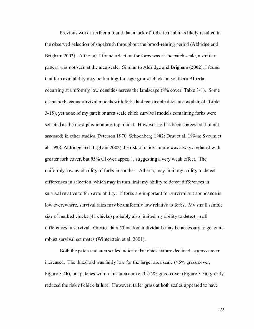
Previous work in Alberta found that a lack of forb-rich habitats likely resulted in

the observed selection of sagebrush throughout the brood-rearing period (Aldridge and

Brigham 2002). Although I found selection for forbs was at the patch scale, a similar

pattern was not seen at the area scale. Similar to Aldridge and Brigham (2002), I found

that forb availability may be limiting for sage-grouse chicks in southern Alberta,

occurring at uniformly low densities across the landscape (8% cover, Table 3-1). Some

of the herbaceous survival models with forbs had reasonable deviance explained (Table

3-15), yet none of my patch or area scale chick survival models containing forbs were

selected as the most parsimonious top model. However, as has been suggested (but not

assessed) in other studies (Peterson 1970; Schoenberg 1982; Drut et al. 1994a; Sveum et

al. 1998; Aldridge and Brigham 2002) the risk of chick failure was always reduced with

greater forb cover, but 95% CI overlapped 1, suggesting a very weak effect. The

uniformly low availability of forbs in southern Alberta, may limit my ability to detect

differences in selection, which may in turn limit my ability to detect differences in

survival relative to forb availability. If forbs are important for survival but abundance is

low everywhere, survival rates may be uniformly low relative to forbs. My small sample

size of marked chicks (41 chicks) probably also limited my ability to detect small

differences in survival. Greater than 50 marked individuals may be necessary to generate

robust survival estimates (Winterstein et al. 2001).

Both the patch and area scales indicate that chick failure declined as grass cover

increased. The threshold was fairly low for the larger area scale (>5% grass cover,

Figure 3-4b), but patches within this area above 20-25% grass cover (Figure 3-3a) greatly

reduced the risk of chick failure. However, taller grass at both scales appeared to have

122

negative consequences for chick survival (i.e., βGrHgt <1.0, Table 3-19), but threshold

models illustrate habitats are not risky until grass height becomes greater than 35-40 cm

(Figures 3-3b, 3-4c). Female sage-grouse are only ca 50 cm in length (Schroeder et al.

1999) and probably standing no more than 40 cm in height. Thus, grass cover taller than

the birds may obscure their ability to detect and quickly evade predators (Wiebe and

Martin 1998). These fitness cues are recognized by sage-grouse, given that hens with

broods selected only moderately for tall grass cover at both scales evaluated (Table 3-8).

However, despite the reduced risk for chicks in habitats with greater grass cover, sage-

grouse showed strong avoidance of dense grass cover at brood rearing sites. Hens may

be forced to make a trade-off between less risky habitats (tall and thick grass cover with

some sagebrush cover), and having to meet dietary requirements while foraging in more

open mesic habitats with less grass and structural cover that are inherently more risky.

The low availability of mesic forb-rich habitats in Alberta may force hens to spend more

time meeting dietary requirements, putting their chicks and possibly themselves, at

greater risk of predation.

Even though my models were predictive, I did not assess the relationship between

insects and habitat selection or chick survival. Insects represent an important dietary

requirement of sage-grouse chicks (Kerwin 1971; Johnson and Boyce 1990; Drut et al.

1994a; Crawford et al. 2004), and recent research on other prairie grouse species has

illustrated selection for insects in brood habitats (Jamison et al. 2002; Hagen et al. 2004).

Selection of insects in brood rearing habitats needs to be assessed. Given the dietary

limitations of chicks (Johnson and Boyce 1990), the consequences of insect abundance

123

on chick survival should also be investigated, so that appropriate management strategies

can be devised.

6. Conclusions

Sage-grouse are a relatively long-lived grouse species with low reproductive rates

(Bergerud and Gratson 1988), making recruitment vital to population persistence. Thus,

linking habitat requirements to juvenile survival and ultimately recruitment, are important

and necessary information to appropriately identify management needs for the species

(Aldridge and Brigham 2001; Crawford et al. 2004). In these analyses, I only assessed

occurrence and survival using climatic and habitat covariates. However, my top models

were highly predictive, explaining 44-50% of sage-grouse brood habitat selection and

chick survival. This does not dismiss the need to assess brood habitat selection and chick

survival at larger landscape scales, accounting for the potential effects of habitat

fragmentation and human-use features such as roads, oil and gas activities and power

lines.

My models represent the first attempt to assess sage-grouse chick survival as a

function of habitat covariates using a shared frailty proportional hazards model to account

for correlation of marked chicks within broods. I was able to identify threshold levels of

grass cover and grass height necessary to ensure chick survival; providing management

targets for sage-grouse brood rearing habitat in Alberta. I also show weak selection for

forb-rich habitats, despite the uniformly low availability of forbs across the landscape.

Although forbs were not in the top-selected proportional hazards model, chick survival

was positively influenced by increased forb abundance. Further research is required into

these relationships, possibly in larger populations with more variability in forb abundance

124

and where larger sample sizes could be obtained, but the benefits of enhanced forb-rich

habitats should not be dismissed, particularly for the Alberta population. Hens may be

forced into an ecological trap situation (Delibes et al. 2001; Breininger and Carter 2003),

spending larger amounts of time searching for poor quality forbs, which increases the risk

of mortality for chicks, and possibly for hens as well.

I suggest that range management strategies be implemented to enhance cover of

grass and increase the abundance of mesic habitats to enhance forb abundance. Various

alternative grazing strategies and/or alternative strategies such as flooding or irrigation of

rangelands needs to be used as management tools to determine the best strategy for

achieving a heterogeneous mixture of these habitat conditions following adaptive

management approach (Aldridge et al. 2004). Indeed, specific management will likely

vary on a site by site basis and considerations for other seasonal habitat requirements

(i.e., winter, nesting, lekking, and summer habitat) needs to be recognized. These

management actions may take many years (>10 years in some cases) before vegetation

and sage-grouse responses can be suitably assessed (Aldridge et al. 2004; Crawford et al.

2004).

125

Table 3-1. Explanatory habitat variables, means and standard errors (in parentheses) of values used to assess brood occurrence and chick survival for 139 brood sites and 139 paired random locations at the patch (177 m2) and area (707 m2) scales in southeastern Alberta from 2001-2003. When grass was absent, height values were considered zero. Models for brood occurrence were initially fit with parameters above the dashed line, validated on an independent set of data from 1998-2000, and then additional parameters only measured for 2001-2003 data were (below dashed line) were added to the top model. Chick survival data was only collected from 2001-2003, and ForbOth was not used in survival models.

Variable 177 m2 patch scale 707 m2 area scale

code Description Brood Site Random Site Brood Site Random Site

SBint Sagebrush cover (%) estimated using line intercept 6.12 (0.52)

1.76 (0.22) 5.12

(0.42) 1.94

(0.22)

SB Sagebrush cover (%) estimated with a 1m2 quadrat 8.85 (0.67)

2.79 (0.34) 7.05

(0.49) 2.95 (0.30

Bush % cover of all shrub (including sagebrush) estimated with a 1m2 quadrat

11.65 (0.77)

4.82 (0.56) 10.02

(0.65) 5.06

(0.53)

Gr Grass cover (%) estimated with 1m2 quadrat 21.20 (1.15)

20.27 (1.30) 21.69

(1.14) 20.65 (0.28)

GrHgt Mean maximum Gr Hgt (cm) within each 1m2 quadrat 35.82 (1.20)

30.50 (1.20) 35.38

(13.40) 30.66 (1.15)

Forb Forb cover (%) estimated with 1m2 quadrat 8.88 (0.77)

8.07 (0.72) 8.69

(0.70) 8.01

(0.72)

ForbOth Unpalatable (Other) forb cover (%) estimated with a 1m2 quadrat

0.60 (0.10)

0.94 (0.12) 0.62

(0.08) 0.94

(0.11)

Robel Visual obstruction reading (height in cm) measured at 2m from pole

10.30 (0.58)

4.95 (0.48) 9.16

(0.46) 5.20

(0.47)

Resid Residual grass cover (%) estimated using a 1m2 quadrat

3.61 (0.38)

3.62 (0.38) 3.63

(0.37) 3.65

(0.37)

Litter Estimate of the cover (%) of litter build up (dead organic matter) using 1m2 quadrat

21.20 (1.02)

16.86 (0.92) 21.22

(0.99) 17.27 (0.87)

126

Table 3-2. Shrub and herbaceous component models used to generate a prior candidate brood occurrence models based on 139 brood sites and 139 paired random nest locations in southeastern Alberta from 2001-2003 at the patch (177 m2) and area (707 m2) scales are shown in (a). Each of the six shrub and herbaceous component models were combined into 36 different initial candidate models (b).

Shrub Component Variables Herbaceous Component Variables

SB GrSB + SB2 Gr + GrHgt Bush Gr + Forb Bush + Bush2 Gr + GrHgt + Forb SBint Forb + GrHgt SBint + SBint2 Gr + GrHgt + Forb + ForbOth

a) b)

# Structure for Sagebrush Quadrat Models # Structure for Bush Models # Structure for Sagebrush Intercept Models

1- SB + Gr 13- Bush + Gr 25- SBint + Gr

2- SB + SB2 + Gr 14- Bush + Bush2 + Gr 26- SBint + SBint2 + Gr

3- SB + Gr + GrHgt 15- Bush + Gr + GrHgt 27- SBint + Gr + GrHgt

4- SB + SB2 + Gr + GrHgt 16- Bush + Bush2 + Gr + GrHgt 28- SBint + SBint2 + Gr + GrHgt

5- SB + Gr + Forb 17- Bush + Gr + Forb 29- SBint + Gr + Forb

6- SB + SB2 + Gr + Forb 18- Bush + Bush2 + Gr + Forb 30- SBint + SBint2 + Gr + Forb

7- SB + Gr + GrHgt + Forb 19- Bush + Gr + GrHgt + Forb 31- SBint + Gr + GrHgt + Forb

8- SB + SB2 + Gr + GrHgt + Forb 20- Bush + Bush2 + Gr + GrHgt + Forb 32- SBint + SBint2 + Gr + GrHgt + Forb

9- SB + Forb + GrHgt 21- Bush + Forb + GrHgt 33- SBint + Forb + GrHgt

10- SB + SB2 + Forb + GrHgt 22- Bush + Bush2 + Forb + GrHgt 34- SBint + SBint2 + Forb + GrHgt

11- SB + Gr + GrHgt + Forb + ForbOth 23- Bush + Gr + GrHgt + Forb + ForbOth 35- SBint + Gr + GrHgt + Forb + ForbOth

12- SB + SB2 + Gr + GrHgt + Forb + ForbOth 24- Bush + Bush2 + Gr + GrHgt + Forb + ForbOth 36- SBint + SBint2 + Gr + GrHgt + Forb + ForbOth

127

Table 3-3. Model structure of additional parameters added to the top AICc-selected for brood occurrence modeling. All 139 brood sites and 139 paired random nest locations in southeastern Alberta from 2001-2003 at the patch (177 m2) and area (707 m2) scales were used.

Model # Structure for 2001-2003 additional parameter models

Top # (Top AICc-selected model for any given scale)

Top #-1 (Top model ) + Robel

Top #-2 (Top model ) + Resid

Top #-3 (Top model ) + Litter

Top #-4 (Top model ) + Robel + Resid

Top #-5 (Top model ) + Robel + Litter

Top #-6 (Top model ) + Resid + Litter

Top #-7 (Top model ) + Robel + Resid + Litter

128

Table 3-4. Explanatory climate variables and models used to assess chick survival for 41 radio-marked chicks from 22 different broods in southeastern Alberta from 2001-2003. Due to small sample sizes, a priori climate models consisted of single parameters only. The asterisk (*) indicates that the GDD model was dropped due to violations of the proportional hazards assumption.

Model # Variable code Description

*1- GDD Cumulative growing degree days (above 5ºC) since 01-March up to the given date for that specific year

2- Sp_PPT_Cumm Cumulative growing season (since 01 – March) precipitation for that specific year

3- Dry_Index An overall dryness index, calculated as the GDD (above) divided by Sp_PPT_Cumm (above)

4- Sp_PPT_Prior Total spring (April through June) precipitation for the spring prior to that specific year

5- Sp-Su_PPT_Prior Total spring and summer precipitation (April though August) of the year prior to that specific year

6- Tot_PPT_Prior Total precipitation for the full calendar year prior to that specific year

7- GDD_Prior Total growing degree days (above 5ºC) from March through August for the year prior to that specific year

129

Table 3-5. Candidate models used to identify the best predictive shrub and herbaceous models predicting sage-grouse chick survival for 41 radio-marked chicks from 22 different broods in southeastern Alberta from 2001-2003. Due to small sample sizes, and in order to develop models with combined components, I limited herbaceous component models to two variables, and modeled each shrub component as a linear or quadratic function. I did not have a validation dataset so parameters withheld from after initial validation for brood occurrence were include in my initial candidate survival models. The asterisk (*) indicates that herbaceous model #12 was dropped due to violations of the proportional hazards assumption. Shrub

Model # Shrub Component Variables

Herbaceous Herbaceous Component Model # Variables

1- SB 1- Forb 2- SB + SB2 2- Forb + Gr 3- Bush 3- Forb + Robel 4- Bush + Bush2 4- Forb + Resid 5-

SBint 5- Robel6- SBint + SBint2 6- Robel + GrHgt 7- Robel + Resid 8- Gr + GrHgt

9- Resid + GrHgt10- Litter

11- Litter + Forb *12- Litter + Robel 13- Litter + GrHgt

130

Table 3-6. AICc brood occurrence models and Akaike weights (wi) for all models within a cumulative summed AICc weight (∑wi) of 0.90 for 139 brood locations at the patch (177 m2) scale. All model Wald χ2 tests were significant at P < 0.0001. Percent deviance (Dev.) explained indicates the reduction in the log-likelihood from the null model.


Likelihood K AICc ∆i AICc wi ∑ wi Model

Wald χ2 % Dev.

Explained

10 SB + SB2 + Forb + GrHgt 48.252 4 104.803 0.000 0.163 0.163 43.96 49.92

4 SB + SB2 + Gr + GrHgt 48.313 4 104.925 0.121 0.153 0.316 43.97 49.86

3 SB + Gr + GrHgt 49.546 3 105.270 0.467 0.129 0.446 39.40 48.58

9 SB + Forb + GrHgt 49.611 3 105.400 0.597 0.121 0.567 39.41 48.51

8 SB + SB2 + Gr + GrHgt + Forb 47.525 5 105.501 0.698 0.115 0.682 49.15 50.67

7 SB + Gr + GrHgt + Forb 48.854 4 106.007 1.204 0.089 0.771 44.33 49.29

12 SB + SB2 + Gr + GrHgt + Forb + ForbOth 47.469 6 107.574 2.770 0.041 0.812 59.42 50.73

6 SB + SB2 + Gr + Forb 49.720 4 107.739 2.936 0.038 0.849 43.98 48.39

11 SB + Gr + GrHgt + Forb + ForbOth 48.796 5 108.043 3.240 0.032 0.882 55.28 49.35

5 SB + Gr + Forb 51.334 3 108.846 4.043 0.022 0.903 35.23 46.72

131

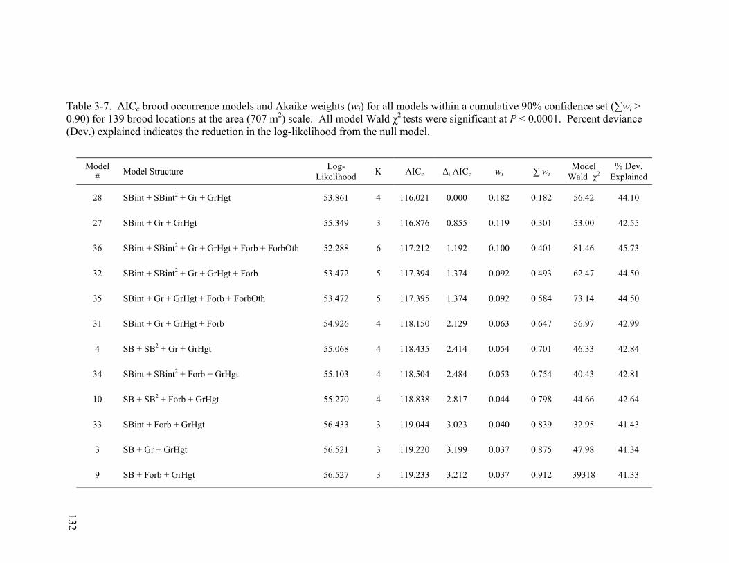
Table 3-7. AICc brood occurrence models and Akaike weights (wi) for all models within a cumulative 90% confidence set (∑wi > 0.90) for 139 brood locations at the area (707 m2) scale. All model Wald χ2 tests were significant at P < 0.0001. Percent deviance (Dev.) explained indicates the reduction in the log-likelihood from the null model.


Likelihood K AICc ∆i AICc wi ∑ wi Model

Wald χ2 % Dev.

Explained

28 SBint + SBint2 + Gr + GrHgt 53.861 4 116.021 0.000 0.182 0.182 56.42 44.10

27 SBint + Gr + GrHgt 55.349 3 116.876 0.855 0.119 0.301 53.00 42.55

36 SBint + SBint2 + Gr + GrHgt + Forb + ForbOth 52.288 6 117.212 1.192 0.100 0.401 81.46 45.73

32 SBint + SBint2 + Gr + GrHgt + Forb 53.472 5 117.394 1.374 0.092 0.493 62.47 44.50

35 SBint + Gr + GrHgt + Forb + ForbOth 53.472 5 117.395 1.374 0.092 0.584 73.14 44.50

31 SBint + Gr + GrHgt + Forb 54.926 4 118.150 2.129 0.063 0.647 56.97 42.99

4 SB + SB2 + Gr + GrHgt 55.068 4 118.435 2.414 0.054 0.701 46.33 42.84

34 SBint + SBint2 + Forb + GrHgt 55.103 4 118.504 2.484 0.053 0.754 40.43 42.81

10 SB + SB2 + Forb + GrHgt 55.270 4 118.838 2.817 0.044 0.798 44.66 42.64

33 SBint + Forb + GrHgt 56.433 3 119.044 3.023 0.040 0.839 32.95 41.43

3 SB + Gr + GrHgt 56.521 3 119.220 3.199 0.037 0.875 47.98 41.34

9 SB + Forb + GrHgt 56.527 3 119.233 3.212 0.037 0.912 39318 41.33

132

Table 3-8. Estimated coefficients (βi), standard errors (shown in parentheses), and 95% confidence intervals for top AICc-selected candidate brood occurrence models in southeastern Alberta. Models were developed on 139 brood sites and 139 paired random locations collected from 2001-2003.


intervals

Variable Patch Scale Model 10

Lower

Upper

Area Scale Model 28

Lower

Upper

SB 0.460 (0.083) 0.296 0.623

SB2 – 0.007 (0.001) – 0.009 – 0.004

SBint

0.757 (0.170) 0.425 1.090

SBint2 – 0.024 (0.008) – 0.039 – 0.009

Gr – 0.040 (0.011) – 0.062 – 0.017

GrHgt 0.058 (0.025) 0.010 0.107 0.115

(0.028) 0.060 0.170

Forb 0.038 (0.021) – 0.004 0.080

133

Table 3-9. Relative variable importance for brood occurrence models (2001-2003), based on the sum of the AICc weights for each variable across all models. (n=139 brood sites and 139 paired random locations). Sagebrush variables below the double line illustrate the strength of the measurement technique (quadrat vs. line intercept) and the importance of the quadratic relationship at each scale. Parameter Model Frequency indicates the frequency for each parameter occurring across all 36 models.

Parameter Model Frequency

177 m2 Patch Scale

707 m2 Area Scale

Bush 6 0.0000 0.0000

Bush + Bush2

6 0.0000 0.0003

SB 6 0.4048 0.1102

SB + SB2 6 0.5298 0.1486

Sbint 6 0.0323 0.3138

Sbint + SBint2 6 0.0330 0.4272

Grass 6 0.6963 0.8261

GrHgt 30 0.9078 0.9900

Forb 24 0.6605 0.6049

ForbOther 24 0.0780 0.2190

All sagebrush (quadrats only) 12 0.9346 0.2587


0.0653 0.7410

All sagebrush (linear) 12 0.4371 0.4239

All sagebrush (quadratic) 12 0.5629 0.5758

Any with sagebrush (both measurements) 24 1.0000 0.9997

134

Table 3-10. Comparison of top AICc-selected brood occurrence models, metrics for overall model significance, model fit, and classification accuracy for both training (139 brood sites from 2001-2003) and testing data (113 brood sites from 1998-2000) across different scales. All model Wald χ2 tests were significant at P < 0.0001. Percent deviance (Dev.) explained indicates the reduction in the log-likelihood from the null model. The area under the receiver operating characteristic curves [ROC (SE)] and the percent correctly classified (PCC) based on the training dataset optimal cut off point were used to assess model classification accuracy.


# AICc Wald χ2 Explained cut-off ROC PCC ROC PCC

177 m2 Patch scale 10 SB + SB2 + Forb + GrHgt 104.803 43.96 49.92 0.5012 0.992

(0.015) 84.17 84.09 (0.027) 76.99

707 m2 Area scale 28 SBint + SBint2 + Gr + GrHgt 116.021 56.42 44.10 0.5014 0.900

(0.017) 79.14 0.8024 (0.029) 70.80

135

Table 3-11. Brood occurrence models and Akaike weights (w ) for additional parameter models at the patch (177 m ) scale for 139 brood and 139 paired random locations based on the initial 2001-2003 AIC -selected top model (#10). Combinations of additional parameters only measured in 2001-2003 for Robel pole, residual grass (Resid) cover, and Litter estimates comprised candidate models. All model Wald χ tests were significant at P < 0.0001. Percent deviance (Dev.) explained indicates the reduction in the log-likelihood from the null model.

2i

c

2


Likelihood K AICc ∆i AICc wi Model

Wald χ2 % Dev.

Explained

10 SB + SB2 + Forb + GrHgt 48.252 4 104.505 0.000 0.364 43.96 49.92

10-1 SB + SB2 + Forb + GrHgt + Robel 47.927 5 105.855 1.503 0.172 47.97 50.26

10-3 SB + SB2 + Forb + GrHgt + Litter 48.089 106.177 1.825 0.146 47.73 50.09

10-2 SB + SB2 + Forb + GrHgt + Resid 48.234 5 106.467 2.115 0.126 47.16 49.94

10-5 SB + SB2 + Forb + GrHgt + Robel + Litter 47.828 6 107.657 3.490 0.064 53.17 50.36

10-4 SB + SB2 + Forb + GrHgt + Robel + Resid 47.923 6 107.846 3.679 0.058 51.65 50.26

10-6 SB + SB2 + Forb + GrHgt + Resid + Litter 48.083 6 108.167 4.000 0.049 51.21 50.09

10-7 SB + SB2 + Forb + GrHgt + Robel + Resid + Litter 47.828 7 109.656 5.708 0.021 57.00 50.36

5

136

Table 3-12. Brood occurrence models and Akaike weights (wi) for additional parameter models at the area (707 m2) scale for 139 brood and 139 paired random locations based on the initial 2001-2003 AICc-selected top model (#10). Combinations of additional parameters only measured in 2001-2003 for Robel pole, residual grass (Resid) cover, and Litter estimates comprised candidate models. All model Wald χ2 tests were significant at P < 0.0001. Percent deviance (Dev.) explained indicates the reduction in the log-likelihood from the null model.


Likelihood K AICc ∆i AICc wi Model

Wald χ2 % Dev.

Explained

28 SBint + SBint2 + Gr + GrHgt 53.861 4 116.021 0.000 0.234 56.42 44.10

28-3 SBint + SBint2 + Gr + GrHgt + Litter 52.897 5 116.245 0.224 0.209 57.36 45.10

28-2 SBint + SBint2 + Gr + GrHgt + Resid 53.191 5 116.834 0.813 0.156 53.81 44.79

28-6 SBint + SBint2 + Gr + GrHgt + Resid + Litter 52.461 6 117.558 1.537 0.109 58.61 45.55

28-1 SBint + SBint2 + Gr + GrHgt + Robel 53.602 5 117.655 1.634 0.103 67.92 44.37

28-5 SBint + SBint2 + Gr + GrHgt + Robel + Litter 52.734 6 118.104 2.084 0.083 69.64 45.27

28-4 SBint + SBint2 + Gr + GrHgt + Robel + Resid 52.985 6 118.606 2.585 0.064 68.06 45.01

28-7 SBint + SBint2 + Gr + GrHgt + Robel + Resid + Litter 52.314 7 119.483 3.463 0.041 70.90 45.70

137

Table 3-13. AICc-selected climate variable proportional hazards chick survival models and Akaike weights (wi) for 41 chicks from 2001-2003. The Wald χ2 is an estimate of the fit of the model to the data, and K indicates the number of model parameters estimated, which includes the covariates and the estimate of the random effect (Theta). Theta is the estimate of the shared frailty variance and the P value for the likelihood ratio tests (LR) for the significance of the correlation is presented. Percent deviance (Dev.) explained indicates the reduction in the log-likelihood from the null model.

Model # Model Structure Theta Estimate

LR P value

Log-Likelihood K AICc ∆i AICc wi

Model Wald χ2

Model χ2 P value

% Dev. Explained

3 Dry_Index 0.314 0.283 72.46845 2 149.508 0.000 0.340 3.48 0.062 10.97

4

Sp_PPT_Prior 0.494 0.193 73.28808 2 151.148 1.639 0.150 1.45 0.229 4.68

5 Sp-Su_PPT_Prior 0.495 0.193 73.29075 2 151.153 1.645 0.150 1.44 0.230 4.66

6 Tot_PPT_Prior 0.527 0.184 73.35259 2 151.277 1.768 0.141 1.27 0.260 4.16

7 GDD_Prior 0.549 0.178 73.39109 2 151.354 1.845 0.135 1.17 0.280 3.86

2 Sp_PPT_Cumm 0.960 0.086 73.86298 2 152.297 2.789 0.084 0.00 0.995 0.00

138

Table 3-14. AICc-selected shrub variable proportional hazards chick survival models and Akaike weights (wi) for all models at the 177 m2 patch and 707 m2 area scales for 41 chicks from 2001-2003 in southeastern Alberta. The Wald χ2 indicated the fit of the model to the data, and K indicates the number of model parameters estimated, which includes the covariates and the estimate of the random effect (Theta). Theta is the estimate of the shared frailty variance and the P value for the likelihood ratio tests (LR) for the significance of the correlation is presented. Percent deviance (Dev.) explained indicates the reduction in the log-likelihood from the null model.

Model # Shrub Model Structure

Theta Estimate

LR P value


Model Wald χ2

Model χ2 P value

% Dev. Explained

177 m2 Patch Scale

1 SB <0.001 0.437 72.022 2 148.616 0.000 0.441 6.13 0.013 14.22

5

SBint 0.052 0.483 72.854 2 150.279 1.663 0.192 3.96 0.047 8.07

2 SB + SB2 <0.001 0.500 71.974 3 151.149 2.532 0.124 5.91 0.052 14.56

3 Bush 0.777 0.158 73.363 2 151.298 2.682 0.115 1.08 0.30 4.08

4 Bush + Bush2 0.805 0.169 72.522 3 152.244 3.628 0.072 2.60 0.272 10.57

6 SBint + SBint2 <0.001 0.466 72.777 3 152.755 4.138 0.056 4.25 0.120 8.65

707 m2 Area Scale

6 SBint + SBint2 0.348 0.342 70.795 3 148.790 0.000 0.346 6.09 0.048 22.56

4 Bush + Bush2 0.805 0.154 71.455 3 149.924 1.134 0.196 4.34 0.114 9.42

1

SB 0.059 0.475 72.676 2 150.111 1.321 0.179 4.30 0.038 18.18

2 SB + SB2 0.109 0.455 72.034 3 151.046 2.257 0.112 4.65 0.098 5.08

5 SBint 0.326 0.351 73.237 2 151.267 2.478 0.100 2.02 0.155 14.14

3 Bush 0.871 0.125 73.759 2 152.089 3.300 0.066 0.22 0.636 0.86

139

Table 3-15. AICc-selected herbaceous variable proportional hazards chick survival models and Akaike weights (wi) for all models at the 177 m2 patch scale for 41 chicks from 2001-2003 in southeastern Alberta. The Wald χ2 indicated the fit of the model to the data, and K indicates the number of model parameters estimated, which includes the covariates and the estimate of the random effect (Theta). Theta is the estimate of the shared frailty variance and the P value for the likelihood ratio tests (LR) for the significance of the correlation is presented. Percent deviance (Dev.) explained indicates the reduction in the log-likelihood from the null model.

Model # Shrub Model Structure Theta Estimate

LR P value


Model Wald χ2

Model χ2 P value

% Dev. Explained

8 Gr + GrHgt 0.215 0.352 71.403 3 150.007 0.000 0.300 4.76 0.093 18.53

2 Forb + Gr <0.001 0.500 72.106 3 151.412 1.405 0.149 4.83 0.089 13.62

1

Forb 0.798 0.110 73.562 2 151.696 1.689 0.129 0.60 0.439 2.47

5 Robel 0.923 0.091 73.831 2 152.234 2.227 0.098 0.06 0.801 0.26

10 Litter 0939 0.099 73.859 2 152.290 2.283 0.096 0.01 0.930 0.03

4 Forb + Resid 0.403 0.351 73.399 3 153.998 3.991 0.041 1.35 0.509 3.79

11 Litter + Forb 0.800 0.115 73.562 3 154.324 4.318 0.035 0.60 0.742 2.48

3 Forb + Robel 0.798 0.110 73.562 3 154.325 4.318 0.035 0.60 0.741 2.47

6 Robel + GrHgt 0.909 0.100 73.647 3 154.494 4.487 0.032 0.43 0.808 1.78

9 Resid + GrHgt 0.789 0.170 73.695 3 154.590 4.583 0.030 0.37 0.832 1.39

7 Robel + Resid 0.723 0.190 73.753 3 154.706 4.700 0.029 0.29 0.867 0.91

13 Litter + GrHgt 0.976 0.096 73.780 3 154.759 4.752 0.028 0.17 0.920 0.69

140

Table 3-16. AICc-selected herbaceous variable proportional hazards chick survival models and Akaike weights (wi) at the 707 m2 area scale for 41 chicks from 2001-2003. The Wald χ2 indicated the fit of the model to the data, and K indicates the number of model parameters estimated, which includes the covariates and the estimate of the random effect (Theta). Theta is the estimate of the shared frailty variance and the P value for the likelihood ratio tests (LR) for the significance of the correlation is presented. Percent deviance (Dev.) explained indicates the reduction in the log-likelihood from the null model.

Model # Shrub Model Structure Theta Estimate

LR P value


Model Wald χ2

Model χ2 P value

% Dev. Explained

8 Gr + GrHgt 0.296 0.307 72.004 3 151.208 0.000 0.202 3.70 0.157 14.35

1

Forb 0.779 0.117 73.674 2 151.920 0.713 0.142 0.40 0.529 1.56

5 Robel 0.878 0.099 73.712 2 151.995 0.787 0.136 0.30 0.583 1.25

2 Forb + Gr 0.034 0.483 72.459 3 152.119 0.911 0.128 4.02 0.134 11.04

10 Litter 0.995 0.083 73.838 2 152.248 1.040 0.120 0.05 0.822 0.21

4 Forb + Resid 0.201 0.444 73.524 3 154.248 3.040 0.044 1.61 0.448 2.79

6 Robel + GrHgt 0.843 0.115 73.544 3 154.289 3.081 0.043 0.62 0.734 2.62

3 Forb + Robel 0.779 0.118 73.619 3 154.439 3.231 0.040 0.50 0.777 2.01

11 Litter + Forb 0.805 0.114 73.645 3 154.490 3.282 0.039 0.45 0.800 1.80

7 Robel + Resid 0.745 0.204 73.692 3 154.584 3.376 0.037 0.39 0.822 1.41

13 Litter + GrHgt 1.016 0.083 73.807 3 154.814 3.606 0.033 0.11 0.944 0.47

9 Resid + GrHgt 0.802 0.188 73.809 3 154.817 3.610 0.033 0.14 0.933 0.45

141

Table 3-17. Overall combined candidate proportional hazards chick survival models for 41 radio-marked chicks from 22 different broods at the patch (177 m2) and area (707 m2) scales in southeastern Alberta from 2001-2003. The top Climate, Shrub, and Herbaceous (Herb) models were used at each scale for combination models. The top within each group was also considered as candidate models within this set. The model with the combination of ‘sagebrush’ + Dry_Index would not converge on a Maximun Likelihood estimate and was therefore not estimated.

Model # Patch Scale Combination Models Model# Area Scale Combination Models

1st Shrub 1- SB 1st Shrub 1- SBint + SBint2

1st Herb 2- Gr + GrHgt 1st Herb 2- Gr + GrHgt

1st Climate 3- Dry_Index 1st Climate 3- Dry_Index

4- SB + Gr + GrHgt 4- SBint + SBint2 + Gr + GrHgt

5- Gr + GrHgt + Dry_Index 5- Gr + GrHgt + Dry_Index

6- SB + Dry_Index + Gr + GrHgt 6- SBint + SBint2 + Dry_Index + Gr + GrHgt

142

Table 3-18. AICc-selected combined proportional hazards chick survival models and Akaike weights (wi) for all models at the 177 m2 patch and 707 m2 area scales for 41 chicks from 2001-2003 in southeastern Alberta. The Wald χ2 indicated the fit of the model to the data, and K indicates the number of model parameters estimated, which includes the covariates and the estimate of the random effect (Theta). Theta is the estimate of the shared frailty variance and the P value for the likelihood ratio tests (LR) for the significance of the correlation is presented. Percent deviance (Dev.) explained indicates the reduction in the log-likelihood from the null model.

Model # Combined Model Structure Theta Estimate

LR P value

Log- Likelihood K AICc ∆i AICc wi

Model Wald χ2

Model χ2 P value

% Dev. Explained

177 m2 Patch Scale

5 Dry_Index + Gr + GrHgt <0.001 0.500 67.184 4 144.474 0.000 0.650 12.12 0.007 42.68

6 SB + Dry_Index + Gr + GrHgt <0.001 0.500 67.053 5 147.440 2.966 0.148 13.11 0.011 43.30

1

5.533

70.362

SB <0.001 0.437 72.022 2 148.616 4.142 0.082 6.13 0.013 14.22

3 Dry_Index <0.314 0.283 72.468 2 149.508 5.034 0.052 3.48 0.062 10.97

2 Gr + GrHgt 0.215 0.352 71.403 3 150.007 0.041 4.76 0.093 18.53

4 SB + Gr + GrHgt 0.001 0.500 4 150.829 6.355 0.027 8.18 0.042 25.31

707 m2 Area Scale

6 SBint + SBint2 + Dry_Index + Gr + GrHgt 0.314 0.283 63.377 5 140.087 0.000 0.905 16.74 0.005 58.27

1

0.296

SBint + SBint2 0.348 0.342 70.795 2 146.161 6.074 0.043 6.09 0.048 22.56

5 Dry_Index + Gr + GrHgt 0.034 0.483 68.299 4 146.704 6.617 0.033 10.55 0.014 37.10

3 Dry_Index 0.779 0.117 72.468 2 149.508 9.421 0.008 3.48 0.062 10.97

4 SB + Gr + GrHgt 0.878 0.099 69.893 4 149.892 9.805 0.007 7.49 0.112 28.17

2 Gr + GrHgt 0.307 72.003 3 151.208 11.121 0.003 3.70 0.157 14.35

143

Table 3-19. Estimated hazard ratios (exponentiated coefficients - exp[βi]), standard errors (shown in parentheses), and confidence intervals for top AICc-selected candidate proportional hazards chick survival combined models in south-eastern Alberta for 41 chicks from 22 different broods from 2001-2003. The top combined model at both scales had the Dry Index, the Gr + GrHgt Herbaceous component model, and a sagebrush component.



Variable Patch scale Model # 5 Lower Upper Area scale

Model # 6 Lower Upper

Dry_Index 1.441 (0.183) 1.123

1.850 1.707 (0.268) 1.256 2.321

SBint 2.068 (0.549) 1.230 3.479

SBint2 0.941 (0.022) 0.898 0.985

Gr 0.932 (0.026) 0.882 0.985 0.953

(0.031) 0.894 1.017

GrHgt 1.056 (0.021) 1.015 1.098 1.076

(0.027) 1.025 1.130

144

Table 3-20. Relative variable importance for proportional hazards combination chick survival models (2001-2003), based on the sum of the AICc weights for each variable across all models (41 chicks). Parameter Model Freq. indicates the frequency for each parameter occurring across all 6 models.

Patch scale Area scale

Parameter Freq.

Variable Importance Parameter

Freq. Variable

Importance

SB 3 0.2566

Sbint + SBint2

3 0.9553

Gr 4 0.8656 4 0.9484

GrHgt 4 0.8656 4 0.9484

Dry_Index 3 0.8501 3 0.9464

145

0.2

5.5

.75

1C

umul

ativ

e Su

rviv

al

0 20 40 60 80Time (days)

Brood Survival95% Brood CIChick Survival95% Chick CI0

.25

.5.7

51

Cum

ulat

ive

Surv

ival

0 20 40 60 80Time (days)

0.2

5.5

.75

1C

umul

ativ

e Su

rviv

al

0 20 40 60 80Time (days)

Brood Survival95% Brood CIChick Survival95% Chick CI

Brood Survival95% Brood CIChick Survival95% Chick CI

Figure 3-1. Comparison of Kaplan Meier cumulative survival curves with 95% confidence intervals for 26 different sage-grouse broods and 41 radio-marked chicks in southeastern Alberta from 2001-2003. The 41 chicks were from 22 different broods, and chick survival shown here does not take into account the correlation between chicks within a brood (maximum of two chicks marked per brood were marked).

146

0.2

5.5

.75

1C

umul

ativ

e S

urvi

val

0 20 40 60 80Time (days)

Basic KM Model

95% CI (Basic KM Model)

Frailty Model0

.25

.5.7

51

Cum

ulat

ive

Sur

viva

l

0 20 40 60 80Time (days)

Basic KM Model


Frailty Model

Basic KM Model


Frailty Model

Figure 3-2. Kaplan Meier (KM) cumulative chick survival curves for 41 radio-marked sage-grouse chicks from 22 different broods in southeastern Alberta from 2001-2003. The basic KM curve (solid line) does not take into account the correlation of marked chicks within the same brood, whereas the Frailty Model (dashed line) represents that baseline Cox proportional hazard survival (i.e. no covariates) and accounts for lack of independence of siblings within the same brood. 95% confidence intervals could not be generated for the frailty model due to the conditional nature of the Cox model on covariates within the model.

147

0

0.1

0.2

0.3

0.4

0.5

0.6

0.7

0.8

0.9

1

0 5 10 15 20 25 30 35 40 45 50

Grass Cover (%)

Rel

ativ

e H

azar

d

a)

0

0.1

0.2

0.3

0.4

0.5

0.6

0.7

0.8

0.9

1

0 5 10 15 20 25 30 35 40 45 50 55 60

Grass Height (cm)

Rel

ativ

e H

azar

d

b)

0

0.1

0.2

0.3

0.4

0.5

0.6

0.7

0.8

0.9

1

0 1 2 3 4 5 6 7 8 9 10

Dryness index

Rel

ativ

e H

azar

d

c)

0

0.1

0.2

0.3

0.4

0.5

0.6

0.7

0.8

0.9

1

0 5 10 15 20 25 30 35 40 45 50

Grass Cover (%)

Rel

ativ

e H

azar

d

a)

0

0.1

0.2

0.3

0.4

0.5

0.6

0.7

0.8

0.9

1

0 5 10 15 20 25 30 35 40 45 50 55 60

Grass Height (cm)

Rel

ativ

e H

azar

d

b)

0

0.1

0.2

0.3

0.4

0.5

0.6

0.7

0.8

0.9

1

0 1 2 3 4 5 6 7 8 9 10

Dryness index

Rel

ativ

e H

azar

d

c)

Figure 3-3. Threshold response curves for the top AICc-selected model (combined Model #5) at the patch scale (177 m2) for relative risk (hazard) for sage-grouse chicks in southern Alberta. Responses are shown across the 90th percentile of availability for each parameter in the model while holding the other parameters in the model at their mean values; a) grass cover, b) grass height, and c) dryness index.

148

0

0.1

0.2

0.3

0.4

0.5

0.6

0.7

0.8

0.9

1

0 5 10 15 20 25 30 35 40 45 50

Grass Height (cm)

Rel

ativ

e H

azar

d

c)

0

0.1

0.2

0.3

0.4

0.5

0.6

0.7

0.8

0.9

1

0 5 10 15 20

Grass Cover (%)

Rel

ativ

e H

azar

d

b)

0

0.1

0.2

0.3

0.4

0.5

0.6

0.7

0.8

0.9

1

0 1 2 3 4 5 6 7 8 9 10

Sagebrush Cover (%)

Rel

ativ

e H

azar

d

a)

0

0.1

0.2

0.3

0.4

0.5

0.6

0.7

0.8

0.9

1

0 1 2 3 4 5 6 7 8 9 10

Dryness Index

Rel

ativ

e H

azar

d

d)

0

0.1

0.2

0.3

0.4

0.5

0.6

0.7

0.8

0.9

1

0 5 10 15 20 25 30 35 40 45 50

Grass Height (cm)

Rel

ativ

e H

azar

d

c)

0

0.1

0.2

0.3

0.4

0.5

0.6

0.7

0.8

0.9

1

0 5 10 15 20

Grass Cover (%)

Rel

ativ

e H

azar

d

b)

0

0.1

0.2

0.3

0.4

0.5

0.6

0.7

0.8

0.9

1

0 1 2 3 4 5 6 7 8 9 10

Sagebrush Cover (%)

Rel

ativ

e H

azar

d

a)

0

0.1

0.2

0.3

0.4

0.5

0.6

0.7

0.8

0.9

1

0 1 2 3 4 5 6 7 8 9 10

Dryness Index

Rel

ativ

e H

azar

d

d)

Figure 3-4. Threshold response curves for the top AICc-selected model (combined Model #6) at the area scale (707 m2) for relative risk (hazard) for sage-grouse chicks in southern Alberta. Responses are shown across the 90th percentile of availability for each parameter in the model while holding the other parameters in the model at their mean values; a) sagebrush cover estimated with the line intercept method b) grass cover, c) grass height, and d) dryness index.

149

7. Literature Cited

Aldridge, C.L. Assessing chick survival of sage grouse in Canada. 2000. Alberta Sustainable Resource Development, Fish and Wildlife Service. Alberta Species at Risk Report. Edmonton, Alberta, Canada.






Anderson, D.R., K.P. Burnham, and W.L. Thompson. 2000. Null hypothesis testing: problems, prevalence, and an alternative. Journal of Wildlife Management 64: 912-923.

Ball, D.A., S.M. Frost, and A.I. Gitelman. 2004. Predicting timing of downy brome (Bromus Tectorum) seed production using growing degree days. Weed Science 52: 518-524.

Bergerud, A.T. and M.W. Gratson. 1988. Survival and breeding strategies of grouse. Pages 473-577 in A. T. Bergerud and M.W. Gratson, eds. Adaptive strategies and population ecology of northern grouse. University of Minnesota Press, Minneapolis, Minnesota.


Braun, C.E. 1998. Sage grouse declines in western North America: what are the problems? Proceedings of the Western Association of State Fish and Wildlife Agencies 78: 139-156.


150



Burnham, K.P. and D.R. Anderson. 2002. Model selection & multi-model inference: a practical information-theoretic approach. Springer-Verlag, New York, New York, USA.

Burnham, K.P. and G.C. White. 2002. Evaluation of Some Random Effects Methodology Applicable to Bird Ringing Data. Journal of Applied Statistics 29: 245-264.

Canfield, R.H. 1941. Application of the line interception method in sampling range vegetation. Journal of Forestry 39: 388-394.


Compton, B.W., J.M. Rhymer, and M. Mccollough. 2002. Habitat selection by wood turtles (Clemmys Insculpta): an application of paired logistic regression. Ecology 83: 833-843.



Connelly, J.W., K.P. Reese, and M.A. Schroeder. 2003. Monitoring of greater Sage-grouse habitats and populations. University of Idaho, Moscow, ID, College of Natural Resources Experiment Station.




Crawford, J.A. and R.S. Lutz. 1985. Sage grouse population trends in Oregon, 1941-1983. Murrelet 66: 69-74.

151



Donovan, T.M. and F.R. Thompson. 2001. Modeling the ecological trap hypothesis: a habitat and demographic analysis for migrant songbirds. Ecological Applications 11: 871-882.

Drut, M.S., J.A. Crawford, and M.A. Gregg. 1994a. Brood habitat use by sage grouse in Oregon. Great Basin Naturalist 54: 170-176.

Drut, M.S., W.H. Pyle, and J.A. Crawford. 1994b. Technical note: diets and food selection of sage grouse chicks in Oregon. Journal of Range Management 47: 90-93.

Dunn, P.O. and C.E. Braun. 1986. Summer habitat use by adult female and juvenile sage grouse. Journal of Wildlife Management 50: 228-235.



Flint, P.L., K.H. Pollock, D. Thomas, and J.S. Sedinger. 1995. Estimating prefledging survival - allowing for brood mixing and dependence among brood mates. Journal of Wildlife Management 59: 448-455.

Gill, R.B. 1966. Weather and sage grouse productivity. Colorado Game, Fish and Parks Department, Denver, Colorado, Outdoor Inormation Leaflet 37.


Hagen, C.A., B.E. Jamison, K.M. Giesen, and T.Z. Riley. 2004. Guidelines for managing lesser prairie-chicken populations and their habitats. Wildlife Society Bulletin 32: 69-82.

Harris, W.C., K.J. Lungle, B. Bristol, D. Dickinson, D. Eslinger, P. Fargey, S.M. McAdam, T. Poirier, and D. Scobie. 200. Canadian Sage Grouse Recovery Strategy

Hosmer, D.W. and S. Lemeshow. 1999. Applied survival analysis: regression modeling

152

of time to event data. John Wiley & Sons, Inc., New York, New York, USA.


Jamison, B.E., R.J. Robel, J.S. Pontius, and R.D. Applegate. 2002. Invertebrate biomass: associations with lesser prairie-chicken habitat use and sand sagebrush density in southwestern Kansas. Wildlife Society Bulletin 30: 517-526.

Johnson, C.J., M.S. Boyce, C.C. Schwartz, and M.A. Haroldson. 2004. Modeling survival: application of the Andersen-Gill model to Yellowstone grizzly bears. Journal of Wildlife Management 68: 966-978.


Johnson, G.D. and M.S. Boyce. 1990. Feeding trials with insects in the diet of sage grouse chicks. Journal of Wildlife Management 54: 89-91.

Johnson, G.D. and M.S. Boyce. 1991. Survival, growth and reproduction of captive-reared sage grouse. Wildlife Society Bulletin 19: 88-93.

June, J.W. Wyoming sage grouse population measurement. Proceedings of the Western Association of State Game and Fish Commissioners, Tucson, Arizona 43: 206-211.

Kaplan, E.L. and P. Meier. 1958. Nonparametric-estimation from incomplete observations. Journal of the American Statistical Association 53: 457-481.

Keating, K.A. and S. Cherry. 2004. Use and interpretation of logistic regression in habitat selection studies. Journal of Wildlife Management 68: 774-789.

Kerwin, M.L. 1971. The status, behavior, and ecology of the sage grouse in Saskatchewan. Thesis University of Saskatchewan, Regina, Saskatchewan, Canada.




Manly, B.F.J. and J.A. Schmutz. 2001. Estimation of brood and nest survival: comparative methods in the presence of heterogeneity. Journal of Wildlife Management 65: 258-270.

153


Massot, M., J. Clobert, A. Chambon, and Y. Michalakis. 1994. Vertebrate natal dispersal - the problem of nonindependence of siblings. Oikos 70: 172-176.



Moynahan, B.J. 2004. Landscape-scale factors affecting population dynamics of greater sage-grouse (Centrocercus urophasianus) in north-central Montana, 2001-2004. Dissertation, University of Montana, Missoula, Montana USA.



Patterson, R.L. 1952. The sage grouse in Wyoming. Sage Books, Inc, Denver, Colorado, USA.

Pendergast, J.F., S.J. Gange, M.A. Newton, M.J. Lindstrom, M. Palta, and M.R. Fisher. 1996. A survey of methods for analyzing clustered binary response data. International Statistical Review 64: 89-118.

Peterson, J.G. 1970. The food habits and summer distribution of juvenile sage grouse in central Montana. Journal of Wildlife Management 34: 147-155.

Pitman, J.C. 2003. Lesser prairie-chicken nest site selection and success, juvenile gender determination and growth, and juvenile dispersal in southwestern Kansas. Thesis, Kansas State University, Manhattan, Kansas USA.

Pollock, K.H., S.R. Winterstein, C.M. Bunck, and P.D. Curtis. 1989. Survival analysis in telemetry studies: the staggered entry design. Journal of Wildlife Management 53: 7-15.

Robel, R.J., J.N. Briggs, A.D. Dayton, and L.D. Hulbert. 1970. Relationships between visual obstruction measurements and weight of grasslands vegetation. Journal of

154

Range Management 23: 295-297.

Rosenberg, D.K. and K.S. Mckelvey. 1999. Estimation of habitat selection for central-place foraging animals. Journal of Wildlife Management 63: 1028-1038.

Schoenberg, T.J. 1982. Sage grouse movements and habitat selection in North Park, Colorado. Thesis, Colorado State University, Fort Collins, Colorado, USA.


Schroeder, M.A. 1997. Unusually high reproductive effort by sage grouse in a fragmented habitat in north-central Washington. Condor 99: 933-941.


Schroeder, M.A. and D.A. Boag. 1988. Dispersal in spruce grouse - is inheritance involved. Animal Behaviour 36: 305-307.


STATA 2004. STATA version 8.2. STATA Corporation, College Station, TX, USA.

Sveum, C.M., J.A. Crawford, and W.D. Edge. 1998. Use and selection of brood-rearing habitat by sage grouse in south central Washington. Great Basin Naturalist 58: 344-351.


Therneau, T.M., P.M. Grambsch, and V.S. Pankratz. 2003. Penalized survival models and frailty. Journal of Computational and Graphical Statistics 12: 156-175.




155


Wisdom, M.J., L.S. Mills, and D.F. Doak. 2000. Life stage simulation analysis: estimating vital-rate effects on population growth for conservation. Ecology 81: 628-641.

156

Chapter Four

Linking Occurrence and Fitness: Landscape-scale Nesting and Brood-rearing

Habitats for Greater Sage-Grouse in Southeastern Alberta

1. Introduction

Sagebrush-steppe ecosystems have undergone extensive changes since European

settlement. Today, many of these ecosystems are considered imperilled, facing

continuing fragmentation and degradation (Knick et al. 2003; Connelly et al. 2004).

Increasing threats include conversion to agriculture (Connelly et al. 2004), invasion by

non-native species (Knick et al. 2003; Connelly et al. 2004), energy extraction activities

and developments (Braun et al. 2002; Lyon and Anderson 2003), intense grazing pressure

(Beck and Mitchell 2000; Hayes and Holl 2003; Crawford et al. 2004), and climate

change (Thomas et al. 2004). As a result, sagebrush-steppe dependent species have

experienced drastic range contractions and population declines; one notable example

being sage-grouse (Centrocercus spp.).

Detailed theoretical and empirical models that describe such changes are

necessary to understand the underlying processes determining population persistence.

While numerous local population studies focusing on fine-scale habitat correlations with

various species declines have been conducted, landscape-scale habitat models (Franklin

et al. 2000; Wisdom et al. 2002a; Wisdom et al. 2002b; Akcakaya et al. 2004) or range-

wide analyses addressing processes and patterns of persistence have been attempted for

relatively few species from only a few ecosystems (see Channell and Lomolino 2000;

Mattson and Merrill 2002; Laliberte and Ripple 2004). Only a handful of these studies

157

have integrated population dynamics with landscape-level resources (Wiegand et al.

1998; Akcakaya et al. 2004), with even fewer successfully decomposing models to

critical life stages and addressing landscape-level drivers of fitness (see Breininger et al.

1998; Breininger and Carter 2003; Larson et al. 2004). This is a critical and necessary

component for long-term conservation of many species of concern (Donovan and

Thompson 2001) that allows biologists and managers to suitably assess population

viability (Boyce et al. 1994; Boyce 2001). Ultimately, measures of habitat quality must

link fitness (reproduction and survival; Van Horne 1983; Morrison 2001) to resources to

accurately assess how resources affect population viability. Occurrence or abundance

may not be a good indicator of fitness (Van Horne 1983; Hobbs and Hanley 1990; Tyre et

al. 2001; Morrison 2001), particularly in human-dominated landscapes (Remes 2000;

Bock and Jones 2004), due to the creation of ecological traps. Thus, habitat-linked

population assessments should involve the identification of 1) habitats animals are likely

to use (occurrence), in addition to 2) habitats where animals are likely to be successful

(fitness). Habitat patches where animals are likely to occur and that also have high

reproduction and/or survival measures are referred to as source habitats (Pulliam 1988;

Breininger et al. 1998), whereas habitats with abundant animals but poor fitness have

been referred to as ‘attractive’ sink habitats (Delibes et al. 2001; Breininger and Carter

2003; Larson et al. 2004) or ecological traps (Donovan and Thompson 2001; Battin 2004;

Bock and Jones 2004). Failure to differentiate attractive sinks from source habitats may

result in incorrect assessments of habitat importance, ultimately leading to inappropriate

management strategies. However, the ability to appropriately assess habitat quality,

linking habitat relationships with fitness, is limited by the difficulty in gathering suitable

158

basic life-history information for many species (Donovan and Thompson 2001),

particularly those that have low reproductive rates or are species of special concern.

The ecology of greater sage-grouse (Centrocercus urophasianus; hereafter ‘sage-

grouse’) has been studied for over 100 years (Bond 1900; Burnett 1905; Simon 1940;

Scott 1942), with about 20 years of extensive research on some life-history stages and

various habitat-occurrence relationships (Patterson 1952; Schroeder et al. 1999; Connelly

et al. 2004). Currently, sage-grouse exist in about half of their ‘historic’ range

(Schroeder et al. 2004), with individual populations declining by 15-92% since the early

1970s (Connelly and Braun 1997; Aldridge and Brigham 2001; Connelly et al. 2004).

Many populations are at risk of extirpation, reinforcing the need to appropriately assess

habitat relationships for this species.

Sage-grouse population declines have been linked to low nesting success

(Crawford and Lutz 1985; Aldridge and Brigham 2001; Connelly et al. 2004) and poor

chick survival (Chapter 3; Aldridge and Brigham 2001; Burkepile et al. 2002). Research

has shown that sage-grouse select nesting habitats with greater sagebrush cover and a

more dense herbaceous understory (Aldridge and Brigham 2002), and that nest success is

positively correlated with sagebrush (Chapter 2; Wallestad and Pyrah 1974; Connelly et

al. 1991; Aldridge and Brigham 2002) and tall grass cover (Gregg et al. 1994; Sveum et

al. 1998b; Aldridge and Brigham 2002; Watters et al. 2002; Crawford et al. 2004). Mesic

habitats with abundant forbs are selected as brood-rearing habitats by female sage-grouse

(Chapter 3; Klebenow and Gray 1968; Drut et al. 1994a; Sveum et al. 1998a) as the forbs

and insects associated within these habitats are thought to be necessary for chick survival

(Johnson and Boyce 1991; Drut et al. 1994b). Limited research on survival of individual

159

chicks however has been conducted (Burkepile et al. 2002) and no research has assessed

the links between habitats and chick survival (Chapter 3 the exception), thus far

addressing only occurrence-habitat relationships (Crawford et al. 2004).

Limited research has assessed the potential landscape features driving habitat

selection and fitness. For sage-grouse, other than the recently published greater sage-

grouse conservation assessment (Connelly et al. 2004), which summarized sage-grouse

habitats and threats range-wide, only one study to my knowledge used a habitat-based

landscape approach to assess sage-grouse population persistence within the interior

Columbia basin of the western United States (Wisdom et al. 2002a; Wisdom et al.

2002b),.

Within their current range, the Alberta sage-grouse population has declined 66-

92% since the 1970s (Aldridge and Brigham 2001). This population is isolated from

other populations and inhabits a heavily fragmented landscape, dominated by oil and gas

activities (Braun et al. 2002). Recent extended drought conditions (Aldridge and

Brigham 2003), and the introduction of the West Nile virus (Naugle et al. 2004) pose

additional threats to the viability of this small endangered population (Aldridge and

Brigham 2003), which has only 400-600 birds remaining. Low productivity limits this

population (Aldridge and Brigham 2001; Aldridge and Brigham 2002; Aldridge and

Brigham 2003) and the implementation of long-term habitat management initiatives may

be required before increases occur (Crawford et al. 2004).

I take a 2-stage approach to identifying critical nesting and brood-rearing habitat

for sage-grouse in Alberta at the landscape scale using a Geographic Information System

(GIS). First, I use resource selection functions (RSFs; Manly et al. 2002) to develop

160

spatial models predicting sage-grouse nest and brood occurrence on the landscape.

Secondly, I use Cox proportional hazards survival models (Andersen and Gill 1982) to

identify the most risky habitat for sage-grouse nests and for chicks. I validate the

predictive capacity of these models using independent data sources. Finally, I combine

these two approaches to identify attractive sage-grouse habitats that pose minimal risk of

failure, referred to as primary or secondary source habitats, following Nielsen’s (2005)

classification. Conversely, I refer to ecological trap-type habitats that are attractive to

sage-grouse but pose considerable risk, as primary or secondary sink habitats.

Considering both habitat selection and fitness allows me to identify critical sage-

grouse nest and brood habitats that require protection as well as to identify attractive sink

habitats that require immediate management. I discuss my findings within the context of

potential reclamations or landscape improvements that could result in the transformation

of non-critical habitats or attractive sink habitats into higher quality attractive source

habitats. Furthermore, since 1977, management guidelines for greater sage-grouse

(Braun et al. 1977; Connelly et al. 2000) have suggested that a 3.2-km buffer of habitat

around known lek sites would ensure critical nesting and brood-rearing habitat is

maintained. This buffer distance is based on research that indicates most females

(depending of study site, between 55-100%) will nest ≤3.2 km of lek sites (see Schroeder

et al. 1999). I use my empirical models to assess the effectiveness of this 3.2-km buffer

at protecting critical nest and brood habitat for sage-grouse in Alberta and,

simultaneously, evaluate the effectiveness of the Province of Alberta’s currently

recommended setback guidelines, which suggest that habitats within 1 km of known lek

sites be protected and petroleum activities be limited within this 1-km radius buffer

161

(Scobie and Faminow 2000; Aldridge and Brigham 2003). Despite the fact that the

Province of Alberta currently has no means to legally protect sage-grouse habitats, I hope

that my models provide managers with the necessary tools to begin identifying critical

habitat requirements for sage-grouse in Canada, as required under the federal Species at

Risk Act (SARA).

2. Study area

My study area was located within the dry mixedgrass prairie of southern Alberta

(49° 24’ N, 110° 42’ W, ca 900 m elevation), centred on a core sage-grouse use area

(1,110 km2) within a greater 4,000 km2 region that they occupy (Figure 1). My study

area contains 16 of the 32 historically known display sites (leks). Of these 32 lek sites, 8

are currently used by sage-grouse within the region; 5 occur within my core study area,

one of which has two satellite leks within 900 m of the main lek site. This area averages

19.1°C in the summer months (July-August) and has an annual precipitation of ca 358

mm (Onefour Agriculture and Agri-food Canada Research Station, AAFC-AAC 2004,

unpublished weather data). A large portion of this area is heavily influenced by oil and

gas activities, and while little of the area within the sage-grouse range has been converted

to cropland (108 km2 within the core use area), the surrounding region is dominated by

cultivated lands. Silver sagebrush (Artemisia cana) is the dominant shrub, and there are

variety of different forb species, including pasture sage (A. frigida), several species of

clover (Trifolium spp. and Melilotus spp.), vetch (Astragalus spp), and common

dandelion (Taraxacum officinale). Needle-and-thread grass (Stipa comata), june grass

(Koeleria macrantha), blue grama (Bouteloua gracilis), and western wheatgrass

162

(Agropyron smithii) are the dominant grass species (Coupland 1961; Aldridge and

Brigham 2003).

3. Methods


Female sage-grouse were captured during the breeding season from 5 of 8 known

active leks in southeastern Alberta from 2001 to 2004 and fitted with a 14-g necklace-

style radiotransmitter (RI-2B transmitters; Holohil Systems Ltd.; Carp, ON Canada).

Hens were located every second day using a 3-element Yagi antenna and an R-1000

scanning telemetry receiver (Communications Specialists, Inc. Orange, CA) so that

nesting attempts and nest fate could be assessed (see Chapter 2). Nest initiation and

hatch/failure were estimated as the midpoint between consecutive (every 2-days)

relocations (Manolis et al. 2000) following Aldridge (Chapter 2).

From 2001-2003, if a nest was successful (i.e. ≥1 egg hatched), I captured chicks

by hand as soon as possible after hatch and attached transmitters (BD-2G transmitters;

Holohil Systems Ltd.; Carp, ON Canada) to 2 randomly chosen chicks from each brood

following Burkepile et al. (2002; see Chapter 3 for detailed description). Hens with

broods (2001-2004) and chicks (2001-2003) were relocated every 2 days during the

brood-rearing period. If chick signals could not be located and the hen behaved as

though she had lost her brood (i.e., flocked up), I considered the chicks to have failed on

that date. All nest and brood locations were recorded in Universal Transverse Mercator

Coordinates using a hand held 12 Channel Global Positioning System (Garmin 12 XL

and GPS II Plus; Garmin International Inc., Olathe, KS).

163

3.2. GIS predictor variables

I developed a suite of variables in a geographical information system (GIS) that

may be important as predictors of sage-grouse nest and brood occurrence, as well as

survival of nests and chicks. Broadly, these variables were related to either habitat

characteristics or human influences on the landscape (See Table 4-1 for a detailed

description of each variable and its data source). First, I used a dry mixedgrass plant

community guide based primarily on soil types (Adams et al. 2005) to identify 7 different

greater sage-grouse ecosite range plant communities (B.W. Adams, Alberta Public Lands,

Lethbridge Alberta, pers. comm.). The 8th category included all human altered

landscapes (roads, well pads, urban structures, and cropland). I used dummy variable

coding and indicator contrasts to assess these variables in my models. I generated

variables that represented the proportion of each of habitat class within a 1-km2 moving

window across the landscape. I used a 22 July 2000 Landsat TM Satellite image (Path 39

Row 26) to generate brightness, greenness, and NDVI (Normalized Difference

Vegetation Index) values using a tasselled-cap transformation of the Landsat TM bands

(Crist and Cicone 1984) in the program PCI Geomatica Prime 8.2 (PCI Geomatics 2001).

Brightness is a surrogate identifying exposed bare ground and poor productive soils (Crist

and Cicone 1984), greenness is a surrogate for productivity that has been shown to be

correlated with leaf area index (Crist and Cicone 1984; White et al. 1997), and NDVI is

an alternative vegetation productivity index (Sellers 1985). I also estimated the mean and

standard deviation (SD) of NDVI values (30 m X 30 m pixels) within a 1-km2 moving

window across the landscape, as I thought larger scale influences may be important.

164

Higher SD values should represent more heterogeneous (variable) habitat patches on the

landscape.

The importance of sagebrush in providing nesting habitat (Wallestad and Pyrah

1974; Gregg et al. 1994; Aldridge and Brigham 2002; Crawford et al. 2004) has been

clearly demonstrated, and it may also be selected at brood-rearing sites (Aldridge and

Brigham 2002). I used a digital map of sagebrush produced by Jones et al. (2005) that

was developed from air photo interpretation (Fent 1999) to estimate sagebrush cover

across the landscape. Sagebrush cover is defines as the percent of each landscape

polygon that was covered with sagebrush plants (Jones et al. 2005). I also estimated the

mean sagebrush cover within a 1-km2 moving window. Previous work (Chapters 2, 3)

has shown that sage-grouse may not select for greater sagebrush densities linearly,

selecting for intermediate cover (with a concave selection function), as very thick shrub

cover can limit herbaceous understory and reduce the bird’s ability to detect predators

(Wiebe and Martin 1998). Thus, I assessed selection for sagebrush cover and mean cover

(moving window over a 1-km2 area) as a quadratic function. Jones et al. (2005) also

categorized the density distribution of sagebrush into 12 different classes ranging from a

single plant, to a continuous distribution of sagebrush. I reclassified this distribution

using dummy variables to identify two measures of ‘patchy’ or heterogeneous sagebrush

distribution (see Table 4-1). I also estimated the proportion of patchy sagebrush habitat

within the 1-km2 moving window.

Sage-grouse broods move to more mesic habitats with greater forb (Klebenow

and Gray 1968; Drut et al. 1994a; Sveum et al. 1998a) and insect (Johnson and Boyce

1991; Drut et al. 1994b) abundance. Thus, I used a soil-moisture index called compound

165

topographic index (CTI), which has been shown to be correlated with soil moisture and

nutrients (Gessler et al. 1995). CTI was derived from a digital elevation model using a

script in ArcGIS 8.3 (ESRI 2002) developed by Evans (2002). Similar to my lines of

inference for NDVI, I also calculated measures of the mean CTI and the variability in

CTI (SD) within a 1-km2 moving widow (Table 4-1). In addition, I generated a distance

to the nearest natural permanent or semi-permanent water source (Table 4-1).

Anthropogenic landscape features included the distance to roads, trails, oil well

sites, crop and urban areas, as well as a density measure for each variable calculated as

the linear km per km trails, the number of well sites within a 1-km

moving window, and the proportion of the area that was either crop (cultivated lands) or

urban (town, farmstead, energy infrastructure) within a 1-km oving window. It has

been suggested that the noise and human activity associated with road and oil wells may

be avoided by (Braun et al. 2002), or have negative consequences (Lyon and Anderson

2003), for sage-grouse. Thus, I also summed the number of pixels classified as either

roads or well sites, that were visible from any given cell on the landscape within 250,

500, and 1,000 m. I used a view-shed analyses tool developed by H. Beyer (University of

Alberta, Edmonton, Alberta, pers. comm.) together with a digital elevation map (DEM) to

generate these data. I assumed that well sites were 9 m in height, and the average vehicle

driving down a road was 2 m in height, for visibility purposes. In 2001, there were ~1,890

water impediments (dams, dugouts, dam-dugout combinations, and a few irrigation

berms/canals and wells) identified within the range of sage-grouse; two thirds of which are not

registered or licensed impediments (McNeil and Sawyer 2003). To assess the role that these

features might play in influencing habitat selection by sage-grouse, I generated a distance-to

2 for roads and 2

2 m

166

and density measure for these water impediments (Table 4-1). The final anthropogenic

variables were a distance and density measure (proportion of habitat within 1-km

human habitat (roads, oil wells, urban), and what I called any non-natural edge habitat (roads,

oil wells, urban and crop).

2 window) for

3.3. Data Analyses


I began model development by conducting univariate analyses for all predictor

variables (Hosmer and Lemeshow 2000), using P < 0.25 based on a Wald z statistic as a

cut off for potential inclusion in my preliminary multivariate model. I assessed each

variable for outliers and non-linearities (Hosmer and Lemeshow 1999; Hosmer and

Lemeshow 2000). If two parameters were correlated (r > |0.6|), I retained the variable

with the smallest P-value. I then began assessment of the full multivariate model,

dropping the least significant parameter (i.e. largest P value), refitting the reduced model

and repeating the process until all remaining parameters were significant at α = 0.05

(Hosmer and Lemeshow 1999; Hosmer and Lemeshow 2000). I tested for

multicollinearity using variance inflation factors (VIF; Menard 1995). VIF scores for

individual parameters greater then 10 or mean scores for a given model considerably

larger than 1 were considered problematic (Chatterjee et al. 2000), and variables were

removed if this was the case. All analyses were conducted in STATA 8.2 (STATA

2004).

167

3.3.2. Logistic regression occurrence analyses

I evaluated 3rd-order (Johnson 1980) sage-grouse brood habitat selection using a

design II approach, following individuals to identify a set of used resources, but assessing

availability at the population level (Thomas and Taylor 1990; Erickson et al. 2001). I

assumed that resource selection functions (RSFs) took the form:

w(x) = exp(β1x1 + β 2x2 +……+ β pxp) (4-1),

where w is the RSF for the predictor variables, xi, and the βi’s are coefficient estimates for

each predictor variable estimated using logistic regression following Manly et al.

(2002:151). The RSF is equivalent to the logistic discriminant contrasting the

distributions of used and available locations; if truly an RSF, the w(x) is a number

proportional to the probability of use (Manly et al. 2002; Keating and Cherry 2004). I

present coefficients for occurrence models as unstandardized linear estimates and

standard errors. I generated 5,000 random locations across a 1-km buffer around a 100%

minimum convex polygon surrounding all sage-grouse nest and brood locations

combined (1,110 km2 area), resulting in a density of about 5 available points per km2. I

used the same 5,000 available locations for both nest and brood occurrence analyses. The

5,000 points allowed me to accurately capture availability, but resulted in a much larger

sample of available points (0) than use (1) points. I used an importance weight, which

gave full weighting to use points, but available points received a weighting (down)

proportional to the ratio of sampled use points to available points (STATA 2004; Users

Guide). Thus, weighting effectively adjusts (inflates) the standard errors of the estimates,

and allows for appropriate traditional inferences about standard errors and P-values for

coefficient estimates.

168


I used the Cox proportional hazards regression model (Cox 1972) to assess how

GIS variables affect nest and chick survival. The Cox model allows for left and right

censoring of data (Andersen and Gill 1982; Cleves et al. 2004) and estimates the hazard

rate [h (t|xi)] for an individual ith subject as follows (Cleves et al. 2004):


where βi’s are the regression coefficients for the xi variables and h0 (t) is the baseline

hazard, which is not parameterized and is left unestimated. I present coefficients for all

survival models as hazard ratios (exp[βi]) and standard errors. For chick survival models,

I fit a latent random effect to account for lack of independence of chicks within broods,

estimating a shared frailty Cox proportional hazards model (Therneau et al. 2003; Cleves

et al. 2004; Wintrebert et al. 2005). Aldridge (Chapter 3) has previously shown that

failing to account for this lack of independence will result in inappropriate survival and

coefficient estimates.

I used the Breslow estimation of the continuous-time likelihood calculation

(Cleves et al. 2004) to partition deaths with tied failure times. The proportional hazards

model is a semi-parametric model which assumes that the effects of the covariates on

survival do not change over time, except for ways in which the model is already

parameterized (Cleves et al. 2004). I assessed this assumption (Winterstein et al. 2001)

for my models by testing for non-zero slopes of Schoenfeld residuals and by inspecting

logarithm quadrats of the estimated cumulated hazard functions (Cleves et al. 2004).

Non-zero slopes (χ2 goodness-of-fit test on the Schoenfeld residuals and non-parallel

logarithm plots) indicate violations of the proportional hazards assumption Andersen and

169

Gill 1982; Schoenfeld 1982; Grambsch and Therneau 1994; Cleves et al. 2004). I report

survival estimates as means ± standard errors.

3.3.4. Model assessment and validation

I used a χ2 statistic (Hosmer and Lemeshow 2000) to asses the fit of all final

models, except for the chick shared frailty proportional hazards model, which I used a

Wald χ2 statistic (Hosmer and Lemeshow 1999; Cleves et al. 2004). For survival models,

‘relative’ deviance (reduction in log-likelihood for the given model from the null model)

was estimated as outlined by Hosmer and Lemeshow (1999). In addition, I estimated the

cumulative daily relative risk of failure for top survival models, by summing the

predicted relative hazard for each individual nest or chick and dividing it by the number

of exposure days. I used these predictions to assess the predictive accuracy using

receiver operator characteristic (ROC) estimates (Fielding and Bell 1997). High model

accuracy results in ROC estimates above 0.9, good model accuracy between 0.7 to 0.9,

and values below 0.7 indicate low model accuracy (Swets 1988; Manel et al. 2001). I

used the percent correctly classified (PCC) at the optimal cut-off to estimate of the

predictive capacity of the top occurrence models. PCC ≥ 80% was considered as

excellent prediction and PCC ≥ 70% was considered reasonable model prediction

(Nielsen et al. 2004). I also validated my nest survival model by predicting it to an

independent sample of 38 nests with known fate produced by 31 different females from

1998-2000 (Aldridge and Brigham 2002, Chapter 2). I assessed fit and prediction as

previously described for my model training data. I did not have an independent sample

of data with which to validate the chick survival model, and limited sample sizes (41

chicks) prevented me from folding my data for cross validating (Boyce et al. 2002)

170

purposes. Thus, for both chick and nest survival models, I took the predicted daily

hazard and tested for differences in that rate of failures/deaths (nest or chick) compared to

those that survived (0). If the model was predictive, chicks/nests that failed should have

been exposed to greater daily hazards than those that survived. I used a one-tailed t-test

with unequal variances to test for difference in daily relative hazard rates.

For occurrence models, it is inappropriate to assess model accuracy and predictive

capacity using ROCs and PCC (Boyce et al. 2002), and deviance estimates are not true

measures given use available design. Thus, I predicted the RSF in my GIS to generate

relative index of occurrence scores, ranking habitats pixels into 5 bins, with bin 1 being

the lowest quality bin. I then tested for a significant Spearman-rank correlation between

ranked bins and frequency of used points occurring in each, after adjusting the bin for

habitat availability across the landscape (Boyce et al. 2002). If the model was predictive,

higher ranked bins should contain an increasing number of use points, resulting in a

significant positive correlation between the bin number and area adjusted frequency of

locations within that bin. Again, I validated both occurrence models using training

datasets (2001 to 2004), and performed out-of-sample validation (1998 to 2000) for both

models using an independent sample of 40 nest locations produced by 33 different

females and 151 brood locations from 16 different broods (Aldridge and Brigham 2002,

Chapters 2, 3).

3.4. Development of habitat states

I defined the 5 ranked bins for nest and brood occurrence models as 1) poor, 2)

low, 3) moderate, 4) good, and 5) high occurrence, with good-to-high indices indicating

that sage-grouse were likely to occur there. Similarly, I applied my survival models to

171

my GIS landscape, ranking the predicted relative risk of failure (nest or chick) for the

survival models, into 5 similar risk bins; 1) minimal, 2) low, 3) moderate, 4) high, and 5)

extreme risk of failure. I used these occurrence and risk indices to identify 5 different

habitat states, following the methods of Nielsen (2005). Occurrence bins ranking from

poor to moderate (1-3) were classified as overall low use, and it was assumed that sage-

grouse would be unlikely to occur in those habitats; although I tested this with validation

data. Thus, I refer to bin 5 as primary habitat, and bin 4 as secondary habitat. In my GIS,

I overlaid the respective nest or chick survival model predictions on the occurrence maps.

Primary and secondary habitats falling in areas of moderate-extreme risk (bins 3-5) were

classified as ‘attractive’ sink habitats, or primary and secondary sinks, respectively, and

habitats with low risk (bins 1-2) remained as primary or secondary habitat. I graphically

illustrated these conceptual habitat states in Figure 4-2. Further, I used this approach to

develop maps depicting these habitat sates, summarizing the proportion of nesting and

brood-rearing habitats within each habitat state. Using these models and predictive maps,

I outline potential management strategies that could improve the abundance of high

quality habitats for sage-grouse, and reduce the proportion of attractive sink habitats on

the landscape.

4. Results

From 2001-2004 I located 113 sage-grouse nests which I used for occurrence

modeling (2 nests were found from unmarked females). I used the 111 nests produced by

61 radio-marked females to assess nest survival. Nest survival to hatch (28 days) was

39.4 ± 4.84%. There was no difference in nest survival between years of my study (Log

rank χ23 = 5.50, P = 0.14) and there was no difference in survival between initial (40.2 ±

172

5.7%, n=77) and second nesting attempts (37.5 ± 9.0%, n=34; Log rank χ21 = 0.07, P =

0.79), allowing me to combine all nests when modelling survival with GIS covariates.

From 2001-2004, I identified a total of 669 brood locations from 35 different

sage-grouse broods (19.11 ± 0.60 per brood), which I used to model brood occurrence on

the landscape. From 2001-2003, I radio-marked 41 chicks from 22 different broods.

Chick survival to 56 days using the shared frailty proportional hazards model was 12.3%

(see Figure 3-2 in Chapter 3) and there was significant correlation (at α = 0.10) in the fate

of chicks within broods (θ = 0.96, P = 0.086) use a base model with no covariates.

4.1. Occurrence models

4.1.1. Nest occurrence

After removing all variables with P > 0.25, and accounting for all correlated

variables (r > |0.6|), the preliminary multivariable nest occurrence model contained 13

variables. Stepwise removal of 7 variables based on P-values resulted in a final model

that contained 6 parameters (Table 4-2). I tested for biologically meaningful interactions

between these remaining 6 terms, and interactions with some of the 7 removed variables,

but none of the interactions were significant. Thus, I used the model in Table 4-2 as my

final nest occurrence model. This model had good fit (Likelihood ratio χ26 = 53.62, P <

0.0001). Based on parameters in this model, sage-grouse showed strong avoidance of

badland habitats (βpEco6 = – 3.0573), areas with high proportion of anthropogenic edge

(βpEdge = – 2.8002), and areas with greater brightness values (βBrit2 = – 0.02115).

Conversely, sage-grouse selected nesting habitat that contained large patches (1-km2) of

moderate sagebrush cover (quadratic; βSBmean = 0.1025 + βSBmean2 = – 0.0014), but where

173

the distribution of sagebrush within these patches was heterogeneous (βpSB_patch2 = 1.5251;

Table 4-2).

When I applied this model to the study area (Figure 4-3) and mapped and binned

the landscape it into the 5 habitat bins, only 30% of the landscape was considered to have

a good-to-high likelihood of sage-grouse nesting there. Both the nests (n=113) I used to

build the model (2001-2004) and independent sample of 40 nest sites from 1998-2000

showed an increasing frequency (area-adjusted) of occurrence within the predicted nest

index bins (Figure 4-4), justifying my classification of bins 1-3 as low use habitats.

Although this relationship was not quite linear, Spearman-rank correlations on the area-

adjusted frequencies and bin ranks revealed a significant positive relationship (training

data: rs = 1.00, P < 0.0001; testing data: rs = 1.00, P < 0.0001), suggesting that the RSF

for nest occurrence was approximately proportional to probability of use.

4.1.2. Brood occurrence

The preliminary multivariable brood occurrence model contained 25 variables

that were not correlated and had P-values < 0.25. After sequentially removing the non-

significant variables with the largest P-values, the model contained 15 significant

variables. I again tested for several biologically plausible interactions, but none were

significant at α = 0.05. Thus, I used this 15-variable model as my final brood occurrence

model (Table 4-3) and made inferences and prediction about this model. This model had

good fit (Likelihood ratio χ215 = 583.32, P < 0.0001). Similar to the nest occurrence

model, hens with broods selected for large patches (1-km2) of moderate sagebrush cover

(quadratic; βSBmean = 0.10445 + βSBmean2 = – 0.0010) that contained a patchy distribution of

sagebrush (βpSB_patch2 = 1.7924; Table 4-3). They also showed selection for more mesic

174

types of habitats, selecting for habitats with higher wetness values (βWet = 0.0217) and

higher mean CTI scores (βCTImean = 0.4835), while avoiding habitats with high brightness

values (βBrit = – 0.0076; Table 4-3). Broods avoided habitats associated with a high

density of urban developments (βpUrban = – 64.9741), areas close to cultivated cropland

(βCrop_dist = 0.1525), and habitats composed largely of ecosite plant community type bins 4

(loamy upland sites), 5 (thin break sites), and 6 (badland sites; Table 4-3). Sage-grouse

broods also tended to occur in areas with a greater density of trails (βTr_dens = 0.2336) and

were closer to water impediments than random (βImped_dist = – 0.06305; Table 4-3).

Surprisingly, broods tended to be closer to well sites (βWell_dist = – 0.4087), but at the same

time, they avoided areas with a greater density of visible well sites within 1 km (βvWell_1km

= – 0.2016; Table 4-3).

I applied this 15 parameter brood occurrence model to the study area landscape

(Figure 4-5), binning habitats from poor to high occurrence. Only 20% of habitat falls

within the good-high habitat occurrence bins. The brood occurrence model validated

well, both with the 669 brood locations I used to train the model (rs = 1.00, P < 0.0001)

and with an independent sample of 151 brood sites for 1998-2000 (rs = 1.00, P < 0.0001).

For both datasets, the area-adjusted frequency of occurrence increased with increasing

brood occurrence bin rank (Figure 4-6).

4.2. Proportional hazards survival models

4.2.1. Nest survival

I retained 9 variables for the preliminary multivariate proportional hazards nest

survival model after univariate analysis. After successively removing non-significant

variables and testing for interactions, the final nest survival model contained 3 variables

175

(Table 4-4). Surprisingly, nest failure was independent of human-use features on the

landscape. As was expected, nest failure was greatly reduced in habitats that contained a

heterogeneous mix of sagebrush cover (βSBpch1 = 0.2862; Table 4-4), however, there was

also a slight increase in risk as sagebrush cover in the immediate vicinity of the nest site

increased (βSBcover = 1.0138; Table 4-4). In addition, as the variability in the NDVI

measures increased (NDVI_sd), risk of failure decreased significantly (βNDVI_sd = 10.9 x

10-8; Table 4-4).

While this model had good fit (Likelihood ratio χ23 = 12.94, P < 0.005) and

explained 18.05% of the variation in nest survival, when assessing it with both training

and testing datasets, the model had moderate-low predictive accuracy (ROCtrain = 0.67;

ROCtest = 0.59) and low predictive capacity (PCCtrain = 60.4%; PCCtest = 55.3%). Using

the cumulative daily relative hazard, however, the nest survival model identified failed

nests as being exposed to more risky habitats for the within sample dataset (t102.05 = 3.52,

P < 0.001), but this model had difficulty differentiating failed from successful nests on

the independent sample of 40 nests (22 failures; t24.50 = 0.82, P = 0.21). Nonetheless,

when I applied this final nest survival model to my landscape, ~60% of habitat was

within the moderate-extreme risk categories, in which I predict sage-grouse nests are

likely to fail (Figure 4-7).

4.2.2. Chick survival

Once I removed candidate variables with P > 0.25, I had 7 uncorrelated variables

in the preliminary multivariate chick survival model. No variables were significant (α =

0.05) when they were sequentially removed. However, the last two variables removed

were significant at α = 0.10 (βCTI = 1.1883; βvWell_1km = 1.5219; Table 4-5) and I choose to

176

use these in the final model, given that my chick sample size was small (24 failures of 41

chicks). Based on these parameters, chick failure increases in habitats with a greater

number of visible well sites within 1 km, and surprisingly risk was also greater in habitats

with higher CTI values. Model fit was moderate (Wald χ22 = 5.74, P < 0.057), but while

sample sizes were small, the model had good deviance explained (21.76%), low

predictive accuracy (ROCtrain = 0.67), and but good classification accuracy (PCCtrain =

70.7%). Using only these two parameters, however, my model accurately identified

chicks that failed as being exposed to more risky habitats, having higher cumulative daily

relative hazard rates for my within sample dataset (t38.39 = 3.03, P = 0.002). When I

applied this model to the landscape, areas with oil and gas activities fall into the extreme

risk category, but the majority of the riparian areas (with high CTI) values are also

identified as risky habitats. About 60% of habitat within the study area was identified as

risky for sage-grouse chicks.

4.3. Habitat States

4.3.1. Nest habitat states

By combining the nest occurrence and nest risk models, the majority (70%) of my

1,110 km2 study area was classified as low use or non-critical nesting habitat for sage-

grouse (Figure 4-9). Of the 30% of the landscape I identified with the occurrence model

as having a good-high likelihood of being used as nesting habitat, over half of this habitat

(19%) occurs in high risk areas, with 11.6% of habitat classified as a primary sink and

7.4% classified as secondary sink nesting habitat (Figure 4-9). Only a small portion of

the landscape is primary nesting habitat (8.4%) with just 2.6% of habitat considered

secondary habitat. Using a 3.2-km radius buffer around all known lek sites as a

177

management guideline to protect sage-grouse nesting habitat, this would result in the

protection of 53.9% of critical sage-grouse nesting habitat (57.8% of primary habitats and

40.0% of secondary habitats; Figure 4-10). Using a 1-km radius buffer around all lek

sites following the current protective notation guidelines used by the Province of Alberta,

only 9.9% of critical sage-grouse nesting habitat (11.5% of primary habitat and 4.7% of

secondary habitat) would be protected (Figure 4-10).

4.3.2. Brood habitat states

My brood occurrence maps indicated that there is limited habitat available (20%)

for sage-grouse brood-rearing. In addition, three quarters of that which is available is

high-risk habitat, and classified as habitat sinks (15 of this 20% of the landscape is

classified as a sink; Figure 4-11), leaving only 5% of the landscape as source brood-

rearing habitat (primary habitat plus secondary habitat; Figure 4-11). This may explain

the low chick survival rates of 12.3%. Of the currently available critical brood-rearing

habitat (5% of landscape), a 3.2 km radius buffer around all known leks would result in

the protection of 62% of this critical habitat (77.1% of primary habitat and 52.5% of

secondary habitat; Figure 4-12). A 1-km radius buffer would protect only 9.9% of

currently available critical sage-grouse brood-rearing habitat (16.0% of primary habitat

and 5.7% of secondary habitat; Figure 4-12).

5. Discussion

Sage-grouse in Alberta have declined precipitously since the 1970s (Aldridge and

Brigham 2003), and, similar to other populations, low recruitment appears to be the major

factor driving these declines (Aldridge 2001; Crawford et al. 2004). My landscape-scale

models indicate a limited supply exists of habitats selected by sage-grouse (good-to-high

178

occurrence bins) for this population, with about 30% of the habitat likely to be used for

nesting (Figure 4-3) and only 20% for brood-rearing (Figure 4-5). Of great concern is the

fact that over half of those habitats identified as attractive nesting habitat (19 of 30%) are

considered risky (moderate-to-extreme risk; Figures 4-7) causing an ecological trap

situation (Delibes et al. 2001; Kristan 2003). Therefore, more than half of nesting habitat

used by sage-grouse will not result in successful nesting attempts (Figure 4-9), even

though sage-grouse still choose to occupy those habitat patches. An even greater threat

to recruitment and population persistence may be the brood habitat ecological trap

scenario, with three quarters of the useable brood habitat (15 out of 20% of the

landscape) likely to result in chick failure (Figure 4-8). Poor quality habitats where

animals have low fitness ultimately drive population dynamics (Van Horne 1983;

Morrison 2001). This clearly appears to be the case for this population, which has low

nest success (39%; sage-grouse range 15-86%; Schroeder et al. 1999), and extremely

poor chick survival (12.3%), indicating that recruitment is unlikely to sustain this

population into the near future.

Small improvements to attractive sink habitats can have disproportional changes

in population persistence (Delibes et al. 2001). Thus, small changes targeted at

improving portions of habitat I identify as primary and secondary nest and brood habitat

sinks have the potential to greatly improve nest success and chick survival, and thus,

positively influence recruitment and population viability.

5.1. Nesting habitat

Consistent with my predictions for nest occurrence and previous research at finer

scales (Chapter 2), nests were more abundant in habitat patches (within a 1-km2 area)

179

with moderate sagebrush cover (quadratic). Selection was also strong for large patches

(1-km2) that contained a heterogeneous distribution of sagebrush cover, with continuous

and sparsely distributed sagebrush habitats avoided. Moderate cover and patchy

distributions likely provide suitable overstory shrub cover while allowing for lateral

herbaceous cover required to conceal nests from predators (Wallestad and Pyrah 1974;

Gregg et al. 1994; Wiebe and Martin 1998; Aldridge and Brigham 2002; Crawford et al.

2004). Nest abundance was lower in habitats with high brightness values, suggesting that

habitats with increased bare ground were avoided. This idea is reinforced by strong

avoidance of badland habitats which are characteristic of shorter annual growth cycles

and steep, dry exposed soils that are less productive (B.W. Adams Alberta Public Lands,

Lethbridge, Alberta, pers. comm.). My GIS based techniques were able to identify

course-scale correlates for identifying this lack of herbaceous understory cover that are

important for sage-grouse nesting habitat.

As I predicted, nest failure was greatly reduced in habitats that contained a

heterogeneous mix of sagebrush cover (βSBpch1 = 0.2862), suggesting that limited

sagebrush cover or continuous dense cover resulted in nest failure (Table 4-4).

Conceivably, this might be why I show a slight increase in risk with increasing sagebrush

cover in the immediate vicinity of the nest site (linear increase; βSBcover = 1.0138; Table 4-

4). Risk also was significantly reduced for increasing NDVI_sd measures. The

extremely small nature of the measure is somewhat deceptive, because NDVI index

values were small, ranging from 0.012 to 0.099. Taking the natural logarithm of the

unexponentiated β coefficient (βNDVI_sd = – 18.33) times an increase in the NDVI_sd

index values of 0.01 (about 10% of range for nest sites) indicates that nest survival would

180

increase by about 17% (exp[– 18.33 * 0.01] = 0.833). Thus, the idea that more diverse

heterogeneous habitats reduced risk also was supported by the small hazard ratio for the

NDVI variability measure (Table 4-4).

Surprisingly, the proportion of any single human-use feature within a 1-km2 area

did not enter into my final nest occurrence model, but when roads, well sites, urban

habitats, and cropland were combined into one parameter (pEdge), sage-grouse strongly

avoided nesting in these edge-dominated landscapes. Hens may be responding to

increased predator densities associated with edge-type habitats (Andren and Angelstam

1988; Herkert et al. 2003) and agricultural landscapes (Andren 1992; Kurki et al. 2000),

avoiding these more risky edge habitats that have been shown to negatively impact

prairie grouse populations (Fuhlendorf et al. 2002; Manzer 2004). However, similar to

many other studies assessing fragmentation effects on productivity (Pasitschniak-Arts

and Messier 1995; Svobodova et al. 2004) I found no effect of edge, or other human

features on sage-grouse nest success (Table 4-4). Pitman (2003) found that nest

placement for lesser prairie-chickens (Tympanuchus pallidicinctus) in Kansas were

further from paved roads than at random. In the same area, Hagen (2003) showed that

proximity to human structures greatly reduced habitat suitability, while roads had no

obvious effect. However, neither of these studies addressed fitness relative to

anthropogenic features. The mean proportion of edge habitat within a 1-km2 window

around nests sites was 2.9 ± 0.7%, compared to an average of 10.1 ± 0.3% edge habitat

across the landscape. Thus, females’ strong avoidance of edge habitats (βpEdge = – 2.80)

for nesting likely prevented my ability to detect survival differences relative to these

features.

181

Ecological traps tend to be more prevalent in human dominated landscapes

(Remes 2000; Bock and Jones 2004), with birds failing to recognize these risks in

landscapes in which they did not evolve, such as human-fragmented habitats. Sage-

grouse, however, may recognize some of these habitats as risky, avoiding potential

ecological traps created in human-dominated habitat patches; at least when selecting

nesting habitat. This does not mean that human features have no ill effects on nesting

sage-grouse. Avoidance of these features removes that habitat patch from use by sage-

grouse, and effectively removes habitat within a 564-m radius (1-km2 area) of those

patches as potential nesting habitat (functional habitat loss). This zonal-habitat influence

may be greater, but I did not test the effect of edge habitat density in windows greater

than a 1-km2 area. Even though sage-grouse might recognize and avoid these

anthropogenic threats, half of all high use nesting (good-to-high rank) habitats are still

considered attractive sinks (Figure 4-9); ecological traps driven by habitat features. I

suggest that my maps be used to identify risky nesting habitats, and managers should

focus efforts at improving nest success by establishing a heterogeneous mix of sagebrush

patches in these areas. Management of local range conditions (Crawford et al. 2004)

aimed at enhancing grass and forb understory that improves visual obstruction cover in

these risky nesting areas (Chapter 2) will likely be required to convert into sinks into

source-type habitats. Range conditions should be assessed locally (see Chapter 2) and

grazing could be a tool used to adaptively manage and enhance these habitats (Aldridge

et al. 2004).

182

5.2. Brood-rearing habitat

As predicted, and has been shown at more local scales (Aldridge and Brigham

2002; Chapter 3), sage-grouse also selected for moderate ranges of sagebrush cover at

sites used for brood-rearing. Brood occurrence also was greater in more heterogeneous

sagebrush stands, because these patchy habitats provide cover to reduce predator

efficiency (Wiebe and Martin 1998) but still afford necessary forb resources. Boyce

(1981) demonstrated that sage-grouse were more abundant in patchy habitats containing a

mix of mesic forb-rich foraging areas interspersed within suitable densities of sagebrush

escape cover.

Brooding hens showed strong avoidance of human-dominated landscapes,

avoiding areas closer to cultivated cropland and areas that contained a greater proportion

of urban developments. With the exception of feeding on some cereal crop such as

alfalfa (Patterson 1952), sage-grouse do not regularly use agricultural dominated

landscapes. Cultivation directly removes habitats from the perspective of sage-grouse,

and has been correlated with sage-grouse population declines in Idaho (Leonard et al.

2000).

Conversely, sage-grouse may only partially recognize some ecological cues

related to anthropogenic features that make habitat risky to chicks. Although hens with

broods tended to be closer to oil wells then at random, they avoided habitats with a

greater density of visible oil wells. This relationship may partially be due to the static

nature of my GIS landscape, for which well sites were fixed at the known distribution on

the landscape in 2002. In some cases, sage-grouse broods occurred close to well sites,

but not often in areas with high well densities (Figure 4-5). However, my chick survival

183

model predicts a 1.5 times increase in risk for each additional oil well that is visible

within 1 km of brood locations (see Figure 4-7). As a result, a significant portion of

primary and secondary brood habitat is classified as attractive sink habitats (see Figure 4-

11). I am not suggesting that the well sites are killing sage-grouse, but birds have been

run over by vehicles travelling on the associated roads (C.L. Aldridge, unpublished data),

and raptorial predators, such as golden eagles (Aquila chrysaetos), ferruginous hawks

(Buteo regalis), red-tailed hawks (Buteo jamaicensis), great horned owls (Bubo

virginianus), and others, are often observed perching on the power lines associated with

these well sites, conceivably exposing sage-grouse chicks to an increased risk of

predation. Regardless of the mechanism, chicks have a low probability of survival,

which is further reduced when energy extraction activities dominate the landscape.

Similar to nest occurrence, sage-grouse broods avoided the less productive and

more exposed badland range plant community habitats (pEco6). Broods also showed

strong avoidance of the thin-break range sites (pEco5), and the loamy upland sites

(pEco4; Table 4-3). The thin-break sites are similar to badland habitats, but contain

greater sagebrush cover, and the loamy upland sites are more productive range sites, but

are dominated by various graminoid species, resulting in a lack of shrubs and forbs (B.W.

Adams, Alberta Public Lands, Lethbridge, Alberta, pers. comm.). Thus, while these 2

sites might provide added cover from either sagebrush or dense grass cover, they lack the

forb component required by sage-grouse broods.

Sage-grouse broods selected for more mesic habitats. This was reflected in brood

occurrence being associated with lower brightness values, and higher mean CTI and

wetness values (Table 4-3). These habitats are likely required for birds to meet dietary

184

requirements, as forb (Klebenow and Gray 1968; Drut et al. 1994a; Sveum et al. 1998a)

and insect abundance is enhanced in these habitats (Johnson and Boyce 1991; Drut et al.

1994b). Hens also chose to be closer to water impediments on the landscape. The effect

of altered water hydrology on the vegetation productivity, composition, and distribution

within this xeric ecosystem needs to be investigated. Removing some of these

impediments on the landscape may effectively return water to the system, and recharge

some of these former mesic sites, rather than retaining water behind a dam or in a dugout.

This could be tested as an adaptive management experiment (Chapter 5; Aldridge et al.

2004), which would provide useful insights into the hydrology of the dry mixedgrass

system and vegetation responses, and may result in improved abundance and quality of

mesic brood-rearing habitats for sage-grouse.

Although mesic habitats were selected, higher CTI values resulted in increased

risk of chick failure. Excluding the high risk values associated with greater well-site

densities (Figure 4-8), the majority of other high CTI risky habitats occurred in riparian

habitats along creeks and streams. While these habitats are not frequently used by sage-

grouse broods (see Figure 4-5), there may be increased risk with these shrubby riparian

corridors, which often contain a greater concentration of predators (Wilcove 1985). In

Chapter 3, I showed that more mesic forb-rich habitats preferred by sage-grouse broods

tend occur in more risky open habitats. I hypothesized that sage-grouse may be making

trade-offs between habitats that provide protective escape cover and risky open mesic

habitats that provide necessary forage resources. This also could be an additional

explanation for the increased risk of chick failure associated with high CTI values.

Recent droughts could have made these habitats even more risky for sage-grouse chicks,

185

particularly if livestock grazing intensities were not subsequently reduced. These

relationships are poorly understood (Crawford et al. 2004) and need to be investigated

within a long-term adaptive management framework (Aldridge et al. 2004; see Chapter

5).

5.3. Leks as focal points for habitat protection

For all prairie grouse the lek is thought of as the focal point for year-round

activities. Much research has focused on maintaining required habitats surrounding leks

and attempting to identify links between habitat alterations and lek dynamics (Merrill et

al. 1999; Niemuth 2000; Woodward et al. 2001; Fuhlendorf et al. 2002; Niemuth and

Boyce 2004). However, my approach of modeling and mapping high-quality nesting and

brood rearing habitats suggests that such a heavy focus on habitat protection around lek

sites may not be suitable to ensure the viability of sage-grouse populations. Using the

recommended 3.2-km radius buffer around known (active and inactive) Alberta lek sites

as a guide (Braun et al. 1977; Connelly et al. 2000), only 54% of critical nesting habitat

(primary and secondary habitat; Figure 4-10) and 62% of critical brood habitat (primary

and secondary habitat; Figure 4-12) would be protected. Given the limited availability of

high-quality habitats within this landscape, protecting only 60% of source habitats may

not be enough to ensure that this population remains viable.

Perhaps even more alarming, is the fact that the 1-km radius buffer around lek

sites used by the Province of Alberta (Scobie and Faminow 2000) will protect less than

10% each of critical nesting and brood-rearing habitat. These guidelines need to be

revised to prevent the quick demise of sage-grouse in Alberta. Even if one used the mean

nest-to-closest active lek distance for this population (4.9 ± 0.28 km, n =153, C.L.

186

Aldridge unpublished data) as a lek-protection buffer, only about 75% of critical nesting

and brood-rearing habitat would be protected. I suggest a more insightful management

approach, using these models and maps to identify and protect important primary and

secondary nesting and brood-rearing habitats throughout the landscape. Given that sage-

grouse show high fidelity to nesting and brood-rearing areas (C.L. Aldridge, unpublished

data; Fischer et al. 1993; Schroeder and Robb 2003) this approach may be particularly

effective, allowing for direct mitigation within frequently used ‘attractive’ sink habitats,

while limiting the negative effects of rampant energy development in the area. However,

careful attention still needs to be given to managing other seasonal habitat requirements,

such as lekking, summer, and winter habitat, and maintain connectivity between these

habitats.

6. Conclusions

I show that a large proportion of habitats used by sage-grouse for nesting and

brood-rearing pose high risks. Sage-grouse appear to recognize and avoid some of these

risky habitats, but still select for others, apparently resulting in ecological traps. Given

the low nest (39%) and chick (12%) survival, it may not be a question of whether or not

sage-grouse are capable of recognizing the risks, as they do avoid (low occurrence) some

of these more risky habitats. Instead, it may simply be that the majority of habitats they

require present major risks to nests or chicks, either due to anthropogenic causes (i.e.

edge habitat, well-site density) or due to limited ‘natural’ habitat resources. Habitat

quality may have been reduced by altered grazing regimes (Beck and Mitchell 2000;

Crawford et al. 2004), altered fire frequencies (Adams et al. 2004), increases in drought

events (Adams et al. 2004), or global change (Thomas et al. 2004). The causes may be

187

diverse, but high-quality habitats are limiting and the conversion of sink habitats into

sources will enhance the viability of sage-grouse in Alberta.

I propose these models as the framework for evaluating management alternatives

aimed at increasing productivity through addressing habitat-quality issues with a habitat-

based population viability analysis approach (Boyce et al. 1994; Boyce and McDonald

1999). My models should be used to identify priority areas that need to be protected

(primary and secondary habitats). In these habitats, further developments should be

prevented to avoid turning these source habitats into sinks. Where developments

currently exist, such that habitat is an attractive sink for sage-grouse, improvements are

necessary to reduce the risk. Edge-type habitats could be removed, including the removal

or decommissioning of roads, possibly through the sharing of road access between oil

companies. Well sites may need to be removed and well pads reclaimed, to reduce

threats to sage-grouse chicks. Power lines have negative consequences for prairie grouse

(Hagen 2003; I did not directly assess this in my study), and power poles may need to be

capped to reduce the number of accessible perch sites for raptors that prey on sage-

grouse, or buried, which will also reduce fatal sage-grouse-power line collisions (Borell

1939).

On a local scale, management will need to focus on structural cover provided by

sagebrush, grass and forbs, and increasing the abundance of mesic habitats that provide

important food resources (forbs and insects). Indeed, management prescriptions for these

priority areas will have to occur on a site-by-site basis, after appropriate assessments have

been conducted. These models and maps provide managers with the tools to assess and

188

prioritize management needs, as well as to evaluate habitat management strategies in an

adaptive management framework (Chapter 5; Aldridge et al. 2004).

189

Table 4-1. Explanatory GIS raster variables used for 3rd order sage-grouse occurrence and survival models for sage-grouse nests and broods. All variables were first tested univariately in occurrence (logistic regression) and survival (proportional hazards) models. Candidate variables with P < 0.25 were removed, and correlated variables with higher P-values were removed. Data type refers to continuous (cont.) or categorical (cat.) variables. All distance measures are in km.

Variable Data type Description

Brit 30m cont. Brightness generated from a Landsat 7 TM satellite image

Wet 30m cont. NDVI 30m cont. Natural Difference Vegetation Index calculated from a TM satellite image NDVI_avg 30m cont. 2 mNDVI_sd Standard deviation of NDVI within a 1-km2 window

30m cont. Compound Topographic Index (high values = increased moisture) CTI_mean 30m cont. Mean CTI values within a 1-km2 moving window CTI_sd 30m cont. Standard deviation of CTI values within a 1-km2 moving window Well_dist Well_dens 10m cont. Count of energy well sites within a 1-km2 moving window

vWell_500m 30m cont. Count of the number of 30 m pixels within a 500 m radius that are well sites vWell_250m 30m cont. Count of the number of 30 m pixels within a 250 m radius that are well sites Rd_dst 10m cont. Distance to nearest road (any paved or gravel road) Rd_dens Liner km per km2 of roads vRd_1km 30m cont. Count of the number of 30 m pixels within a 1km radius that are road vRd_500m 30m cont. Count of the number of 30 m pixels within a 500 m radius that are road vRd_250m Count of the number of 30 m pixels within a 250 m radius that are road Tr_dst 10m cont. Distance to nearest trail (non-paved or gravelled truck trail) Tr_dens 10m cont. Liner km per km2 of trails Imped_dst Distance to nearest water impediment (dam, dugout, dam-dugout combination)

10m cont. Count of the number of water impediments within a 1-km2 moving window Water_dst 10m cont.

% Sagebrush cover as identified from air photo interpretation SB2 10m cont. SBmean 10m cont. Mean % sagebrush cover within a 1-km2 moving window SBmean2 10m cont. Squared term for SBmean

10m cont. Patchy sagebrush distribution 1- (codes 7, 8, and 9 of Jones et al. 2005) pSB_pch1 10m cont. 2 SB_pch2 10m cont. Patchy sagebrush distribution 2-(codes 7, 8, 9 and 11 of Jones et al. 2005) pSB_pch2 10m cont. Proportion of habitat within a 1-km2 moving window that is SB_pch2

Green 30m cont. Greenness generated from a Landsat 7 TM satellite image Wetness generated from a Landsat 7 TM satellite image

Mean NDVI value within a 1-km oving window 30m cont.

CTI

10m cont. Distance to nearest standing energy well site

vWell_1km 30m cont. Count of the number of 30 m pixels within a 1km radius that are well sites

10m cont.

30m cont.

10m cont. Imped_dens

Distance to the nearest natural permanent or semi-permanent water body SB 10m cont.

Squared term for SB

SB_pch1 Proportion of habitat within a 1-km moving window that is SB_pch1

190

Table 4-1 (continued)

Notes:

Variable Type Description

Crop_dst 10m cont. Distance to nearest cultivated lands pCrop 10m cont. Proportion of habitat within a 1-km2 moving window that is cultivated

pUrban 10m cont. Proportion of habitat within a 1-km2 moving window that is urban (town, ranch, energy compressor station etc.)

Urban_dst 10m cont. Distance to nearest urban developments Eco1 10m cat. Loamy range site with well drained soils, low sagebrush cover Eco2 10m cat. Saline lowlands, swales and depression, spares low sagebrush

Eco3 10m cat. Blowout and overflow sites, solonetzic soils; plant community varies, but higher density of sagebrush

Eco4 10m cat. Loamy upland sites with medium texture soils, fescue & wheatgrasses Eco5 10m cat. Thin break range sites, soils vary, characterized by greater shrub cover Eco6 10m cat. Badlands type habitats with juniper and needle-and-thread-blue grama Eco7 10m cat. Broad, wetland and shrubby (willow, rose, snowberry) riparian habitats

Eco8 10m cat. All altered habitats (urban, crop, wells and roads) see also Hum and Edge below

pEco1 10m cont. Proportion of habitat within a 1-km2 moving window that is Eco1 pEco2 10m cont. Proportion of habitat within a 1-km2 moving window that is Eco2 pEco3 10m cont. Proportion of habitat within a 1-km2 moving window that is Eco3 pEco4 10m cont. Proportion of habitat within a 1-km2 moving window that is Eco4 pEco5 10m cont. Proportion of habitat within a 1-km2 moving window that is Eco5 pEco6 10m cont. Proportion of habitat within a 1-km2 moving window that is Eco6 pEco7 10m cont. Proportion of habitat within a 1-km2 moving window that is Eco7 Hum_dst 10m cont. Distance to any human habitat (roads, wells, urban)

pHum 10m cont. Proportion of habitat within a 1-km2 moving window that is human habitats

Edge 10m cont. Distance to habitat that creates non-natural edge (human above + crop) pEdge 10m cont. Proportion of habitat within 1-km2 moving window that is edge

-TM derived variables were based on a 22 July 2000 Landsat 7 image (Path 39 Row 26) -Digital elevation model derived from 1:50,000 National Topographic Database Contour Lines -Sagebrush, crop, urban, and water base features Jones et al. (2005) -Sagebrush cover is the percent of area within each polygon covered by sagebrush (Jones et al. 2005) -Linear Features based on a 2001 landscape from Alberta Provincial Base features (1:20,000) -Well locations provided by Alberta Energy for the study area as of August, 2002 -Water impediments were mapped based on (McNeil and Sawyer 2003) -Eco1to Eco7 are dry mixedgrasss rangeland ecosite plant community bins after (Adams et al. 2005)

191

Table 4-2. Estimated coefficients (βi) and standard errors (S.E.) for the final nest occurrence model for 113 sage-grouse nests in southeastern Alberta from 2001-2004. 5,000 random points were used to characterise habitat availability and these points were weighted using importance weights such that the available sample was effectively 113 points. P values indicated the significance of the coefficients using a Wald z statistic.

Variable name βi S.E. P

Brit – 0.0215 0.0082 0.009

SBmean 0.1025 0.0401 0.011

SBmean2 – 0.0014 0.0007 0.047

pSB_pch2 1.5251 0.7602 0.045

pEco6 – 3.0573 0.9654 0.002

pEdge – 2.8002 1.3531 0.038

Table 4-3. Estimated coefficients (βi) and standard errors (S.E.) for the final brood occurrence model for 669 sage-grouse brood locations in southeastern Alberta from 2001-2004. 5,000 random points were used to characterise habitat availability and these points were weighted using importance weights such that available sample was effectively 669 points. P values indicated the significance of the coefficients using a Wald z statistic.


Brit – 0.0076 0.0032 0.018

Wet 0.0217 0.0088 0.013

CTI_mean 0.4835 0.0872 < 0.001

Well_dist – 0.4087 0.0446 < 0.001

vWell_lkm – 0.2016 0.0591 0.001

Tr_dens 0.2336 0.0887 0.008

Imped_dist – 0.6305 0.2134 0.003

SBmean 0.1044 0.0175 < 0.001

SBmean2 – 0.0010 0.0003 < 0.001

pSB_pch2 1.7924 0.3703 < 0.001

Crop_dist 0.1525 0.0339 < 0.001

pUrban – 64.9741 18.2819 < 0.001

pEco4 – 1.2791 0.3625 < 0.001

pEco5 – 2.1208 0.3368 < 0.001

pEco6 – 1.8744 0.4931 < 0.001

192

Table 4-4. Estimated hazard ratios (exponentiated coefficients - exp[βi]) and standard errors (S.E.) for the final proportional hazards nest survival model using 111 sage-grouse nest sites in southeastern Alberta from 2001-2004. P values indicated the significance of the coefficients using a Wald z statistic.


NDVI_sd 10.9 *10-8 9.44 0.034

SB 1.0138 0.0052 0.007

pSBpch1 0.2862 0.1784 0.045

Table 4-5. Estimated hazard ratios (exponentiated coefficients - exp[βi]) and standard errors (S.E.) for the shared frailty final proportional hazards chick survival model using 41 sage-grouse chicks from 22 different broods in southeastern Alberta from 2001-2003. P values indicated the significance of the coefficients using a Wald z statistic. The shared Frailty variance estimate was θ = 1.246, P = 0.047.


CTI 1.1883 0.1145 0.073

vWell_1km 1.5219 0.3437 0.063

193

Figure 4-1. Alberta greater sage-grouse study area showing sagebrush density with roads, trails, well pads, and major water bodies. Inset map shows the study area and current range of sage-grouse within Alberta, with major rivers, water bodies, and cities for reference.

194

1

2

3

4

5

6

1 2 3 4 5

Occurrence Index

Ris

k In

dex

5

4

3

2

1

PrimarySink

PrimaryHabitat

Secondary Sink

Secondary Habitat

Low Occurrence

Figure 4-2. A graphic representation of nesting and brood-rearing habitat states for sage-grouse in southeastern Alberta. States include non-critical (low occurrence) habitat, Primary Habitat (high occurrence and low- moderate risk), Secondary Habitat (good occurrence and low-moderate risk), Primary Sink (high occurrence and moderate-extreme risk), and Secondary Sink (high occurrence and moderate-extreme risk). Adapted from Nielsen (2005).

195

Figure 4-3. Relative index of sage-grouse nest occurrence in southeastern Alberta, as determined by a logistic regression nest occurrence model. Good and high index values indicate that sage-grouse are likely to nest in these habitats.

196

0.0

1.0

2.0

3.0

Poor Low Moderate Good High

Nest Habitat Index of Occurrence

Are

a A

djus

ted

Sele

ctio

n R

atio 2001-2004 Training Data

1998-2000 Validation Data

Figure 4-4. Area-adjusted frequency of sage-grouse nest sites in southeastern Alberta falling within nest habitat index of occurrence bins ranked as poor, low, moderate, good, and high. Training data consists of 113 within sample nest sites from 2001-2004 and the Validation sample consists 40 out-of-sample nest sites from 1998-2000.

197

Figure 4-5 Relative index of sage-grouse brood occurrence in southeastern Alberta, as determined by a logistic regression brood occurrence model. Good and high index values indicate that sage-grouse are likely to raise their broods in these habitats.

198

0.0

1.0

2.0

3.0

4.0

5.0

6.0

7.0

Poor Low Moderate Good High

Brood Habitat Index of Occurrence

Are

a A

djus

ted

Sele

ctio

n R

atio 2001-2004 Training Data

1998-2000 Validation Data

Figure 4-6. Area-adjusted frequency of sage-grouse brood sites from southeastern Alberta falling within brood habitat index of occurrence bins ranked as poor, low, moderate, good, and high. Training data consists of 669 within sample brood sites from 2001-2004 and the validation sample consists 151 out-of-sample brood sites from 1998-2000.

199

Figure 4-7. Relative index risk of sage-grouse nest failure in southeastern Alberta, as determined by Cox proportional hazards modelling of nest survival. High and extreme risk values indicated a nest is likely to fail if it occurs in these habitats.

200

Figure 4-8. Relative index risk of sage-grouse chick failure in southeastern Alberta, as determined by Cox proportional hazards modelling of chick survival. High and extreme risk values indicated chicks are likely to die if hens move their broods into these habitats.

201

Figure 4-9. Nesting habitat states for sage-grouse in southeastern Alberta. Non-critical habitat indicates sage-grouse are not likely to nest in those areas. Primary and secondary indicate high and good likelihood of nest occurrence, respectively, and habitats are areas with minimal-low risk of nest failure, whereas sinks are areas with moderate-extreme risk. For example, primary habitat indicates areas where nests are likely to occur (high occurrence values) and be successful (minimal-low risk values), whereas primary sink indicates high occurrence where nests are likely to fail (moderate-extreme risk values).

202

Figure 4-10. Nest habitat states that would be included if a 3.2-km radius buffer around all known lek sites was used to protect sage-grouse nesting habitat, as outlined by Connelly et al. (2000). The 1-km radius buffer represents current protective notations or recommended guidelines used by the province of Alberta to protect critical sage-grouse nesting habitat. The 3.2-km buffer includes 53.9% of Primary and Secondary nesting habitat, whereas the 1-km buffer protects only 9.9% of critical nesting habitat.

203

Figure 4-11. Brood habitat states for sage-grouse in southeastern Alberta. Non-critical habitat indicates sage-grouse are not likely to nest in those areas. Primary and secondary indicate high and good likelihood of brood occurrence, respectively, and habitats are areas with minimal-low risk of chick failure, whereas sinks are areas with moderate-extreme risk. For example, primary habitat indicates areas where broods are likely to occur (high occurrence values) and survive (minimal-low risk values), whereas primary sink indicates high occurrence where chicks are likely to fail (moderate-extreme risk values).

204

Figure 4-12. Brood habitat states that would be included if a 3.2-km radius buffer around all known lek sites was used to protect sage-grouse nesting habitat, as outlined by Connelly et al. (2000). The 1-km radius buffer represents current protective notations or recommended guidelines used by the province of Alberta to protect critical sage-grouse brood-rearing habitat. The 3.2-km buffer includes 62.5% of primary and secondary brood-rearing habitat, whereas the 1-km buffer protects only 9.9% of critical brood habitat.

205

7. Literature Cited

Adams, B.W., L. Poulin-Klein, D. Moisey and R.L. McNeil. 2005. Rangeland plant communities and range health assessment guidelines for the dry mixedgrass natural subregion of Alberta. Rangeland Management Branch, Public Lands Division, Alberta Sustainable Resource Development, Lethbridge, Pub. No. T/040.

Adams, B.W., J. Carlson, D. Milner, T. Hood, B. Cairns, and P. Herzog. Beneficial grazing management practices for sage-grouse (Centrocercus urpohasianus) and ecology of silver sagebrush (Artemisia cana) in southeastern Alberta. 2004. Technical Report, Public Lands and Forest Division, Alberta Sustainable Resource Development. Pub No. T/049.

Akcakaya, H.R., V.C. Radeloff, D.J. Mlandenoff, and H.S. He. 2004. Integrating landscape and metapopulation modeling approaches: viability of the sharp-tailed grouse in a dynamic landscape. Conservation Biology 18: 526-537.


Aldridge, C.L. 2001. Do sage grouse have a future in Canada? Population dynamics and management suggestions. Pages 1-11 in Anonymous eds. Proceedings of the 6th Prairie Conservation and Endangered Species Conference; 22-25 February 2001, Winnipeg, Manitoba, Canada






Andren, H. 1992. Corvid density and nest predation in relation to forest fragmentation - a landscape perspective. Ecology 73: 794-804.

Andren, H. and P. Angelstam. 1988. Elevated predation rates as an edge effect in habitat islands - experimental evidence. Ecology 69: 544-547.

206

Beck, J.L. and D.L. Mitchell. 2000. Influences of livestock grazing on sage grouse habitat. Wildlife Society Bulletin 28: 993-1002.


Bond, F. 1900. A nuptial performance of the sage cock. Auk 17: 325-327.

Borell, A.E. 1939. Telephone wires fatal to sage grouse. Condor 41: 85-86.

Boyce, M.S. 1981. Robust canonical correlation of sage grouse habitat. Pages 152-159 in D.E. Capen, ed. The Use of Multivariate Statistics in Studies of Wildlife Habitat. Rocky Mountain. Forest and Range Experiment Station, Fort Collins, C.O., USA.

Boyce, M.S. 2001. Population viability analysis: development, interpretation, and application. Pages 123-136 in T.M. Shenk and A.B. Franklin, eds. Modeling in Natural Resource Management: Development, Interpretation, and Application. Island Press, Washington.

Boyce, M.S., J.S. Meyer, and L. Irwin. 1994. Habitat-based PVA for the northern spotted owl. Pages 63-85 in D.J. Fletcher and B.I.J. Manly, eds. Statistics in Ecology and Environmental Monitoring. University of Otago Press, Dunedin, CA.

Boyce, M.S., P.R. Vernier, S.E. Nielsen, and F.K.A. Schmiegelow. 2002. Evaluating resource selection functions. Ecological Modelling 157: 281-300.

Braun, C.E., T. Britt, and R.O. Wallestad. 1977. Guidelines for maintenance of sage grouse habitats. Wildlife Society Bulletin 5: 99-106.






207

Burnett, L.E. 1905. The sage grouse, (Centrocercus Urophasianus). Condor 7: 102-105.

Channell, R. and M.V. Lomolino. 2000. Dynamic biogeography and conservation of endangered species. Nature 403: 84-86.

Chatterjee, S., A.S. Hadi, and B. Price. 2000. Regression analysis by example. John Wiley and Sons, New York, New York, USA





Connelly, J.W., W.L. Wakkinen, A.D. Apa, and K.P. Reese. 1991. Sage grouse use of nest sites in southeastern Idaho. Journal of Wildlife Management 55: 521-524.



Crawford, J.A. and R.S. Lutz. 1985. Sage grouse population trends in Oregon, 1941-1983. Murrelet 66: 69-74.


Crist, E.P. and R.C. Cicone. 1984. Application of the tasseled cap concept to simulated thematic mapper data. Photogrammetric Engineering and Remote Sensing 50: 343-352.


Donovan, T.M. and F.R. Thompson. 2001. Modeling the ecological trap hypothesis: a habitat and demographic analysis for migrant songbirds. Ecological Applications 11:

208

871-882.

Drut, M.S., J.A. Crawford, and M.A. Gregg. 1994a. Brood habitat use by sage grouse in Oregon. Great Basin Naturalist 54: 170-176.

Drut, M.S., W.H. Pyle, and J.A. Crawford. 1994b. Technical note: diets and food selection of sage grouse chicks in Oregon. Journal of Range Management 47: 90-93.

ESRI, 2002. Environmental Systems Research Institute. ArcGIS: Release 8.3 [software]. Redlands, California, USA: Environmental Systems Research Institute, 1999–2002.

Fischer, R.A., A.D. Apa, W.L. Wakkinen, K.P. Reese, and J.W. Connelly. 1993. Nesting-area fidelity of sage grouse in southeastern Idaho. Condor 95: 1038-1041.


Evans, J., 2002. Compound topographic index, AML script. Available at ESRI.com support downloads, http://arcscripts.esri.com/details.asp?dbid=11863

Fent, L. 1999. Aerial films and solar angles: influences on silver sagebrush inventory. Journal of Range Management 52: 32-38.



Fuhlendorf, S.D., A.J.W. Woodward, D.M. Leslie, and J.S. Shackford. 2002. Multi-scale effects of habitat loss and fragmentation on lesser prairie-chicken populations of the US Southern Great Plains. Landscape Ecology 17: 617-628.

Gessler, P.E., I.D. Moore, N.J. Mckenzie, and P.J. Ryan. 1995. Soil-landscape modeling and spatial prediction of soil attributes. International Journal of Geographical Information Systems 9: 421-432.



209

Hagen, C.A. 2003. A demographic analysis of lesser prairie-chicken populations in southwestern Kansas: survival, population viability, and habitat use. Dissertation, Kansas State University, Manhattan, Kansas, USA.

Hayes, G.F. and K.D. Holl. 2003. Cattle grazing impacts on annual forbs and vegetation composition of mesic grasslands in California. Conservation Biology 17: 1694-1702.

Herkert, J.R., D.L. Reinking, D.A. Wiedenfeld, M. Winter, J.L. Zimmerman, W.E. Jensen, E.J. Finck, R.R. Koford, D.H. Wolfe, S.K. Sherrod, M.A. Jenkins, J. Faaborg, and S.K. Robinson. 2003. Effects of prairie fragmentation on the nest success of breeding birds in the midcontinental United States. Conservation Biology 17: 587-594.

Kurki, S., A. Nikula, P. Helle, and H. Linden. 2000. Landscape fragmentation and forest composition effects on grouse breeding success in boreal forests. Ecology 81: 1985-1997.


Hosmer, D.W. and S. Lemeshow. 1999. Applied survival analysis: regression modeling of time to event data. John Wiley & Sons, Inc., New York, New York, USA.



Johnson, G.D. and M.S. Boyce. 1991. Survival, growth and reproduction of captive-reared sage grouse. Wildlife Society Bulletin 19: 88-93.

Jones, P.F., R. Penniket, L. Fent, J. Nicholson, and B. Adams. 2005. Silver Sagebrush Community Associations in Southeastern Alberta, Canada. Rangeland Ecology & Management. In press.

Keating, K.A. and S. Cherry. 2004. Use and interpretation of logistic regression in habitat selection studies. Journal of Wildlife Management 68: 774-789.


Knick, S.T., D.S. Dobkin, J.T. Rotenberry, M.A. Schroeder, W.M. Vander Haegen, and C. Van Riper. 2003. Teetering on the edge or too late? Conservation and research issues for avifauna of sagebrush habitats. Condor 105: 611-634.

Kristan, W.B. 2003. The role of habitat selection behavior in population dynamics: source-sink systems and ecological traps. Oikos 103: 457-468.

210

Laliberte, A.S. and W.J. Ripple. 2004. Range contractions of North American carnivores and ungulates. Bioscience 54: 123-138.


Leonard, K.M., K.P. Reese, and J.W. Connelly. 2000. Distribution, movements and habitats of sage grouse Centrocercus Urophasianus on the upper Snake River Plain of Idaho: changes from the 1950s to the 1990s. Wildlife Biology 6: 265-270.

Lyon, A.G. and S.H. Anderson. 2003. Potential gas development impacts on sage grouse nest initiation and movement. Wildlife Society Bulletin 31: 486-491.



Manolis, J.C., D.E. Andersen, and F.J. Cuthbert. 2000. Uncertain nest fates in songbird studies and variation in Mayfield estimation. Auk 117: 615-626.


Mattson, D.J. and T. Merrill. 2002. Extirpations of grizzly bears in the contiguous United States, 1850-2000. Conservation Biology 16: 1123-1136.

McNeil, R.L. and B.J. Sawyer. 2003. Effects of water management practices and precipitation events on sagebrush habitat in southeastern Alberta. Prepared for Alberta Conservation Association and Alberta Sustainable Resource Development by Landwise Inc., Lethbridge, Alberta, Canada


Merrill, M.D., K.A. Chapman, K.A. Poiani, and B. Winter. 1999. Land-use patterns surrounding greater prairie-chicken leks in northwestern Minnesota. Journal of Wildlife Management 63: 189-198.


211


Nielsen, S.E., 2005. Habitat ecology, conservation, and projected population viability of grizzly bears (Ursus arctos L.) in west-central Alberta, Canada. Dissertation, University of Alberta, Edmonton, Alberta, Canada.


Niemuth, N.D. 2000. Land use and vegetation associated with greater prairie-chicken leks in an agricultural landscape. Journal of Wildlife Management 64: 278-286.

Niemuth, N.D. and M.S. Boyce. 2004. Influence of landscape composition on sharp-tailed grouse lek location and attendance in Wisconsin pine barrens. Écoscience 11: 209-217.

Pasitschniak-Arts, M. and F. Messier. 1995. Risk of predation on waterfowl nests in the Canadian prairies: effects of habitat edge and agricultural practices. Oikos 73: 347-355.

Patterson, R.L. 1952. The sage grouse in Wyoming. Sage Books, Inc, Denver Colorado, USA.

PCI Geomatics. 2001. Geomatica Prime: Release 8.2 [software]. Richmond Hill, Ontario, Canada.


Pulliam, H.R. 1988. Sources, sinks, and population regulation. American Naturalist 132: 652-661.

Remes, V. 2000. How can maladaptive habitat choice generate source-sink population dynamics? Oikos 91: 579-582.



212

Schroeder, M.A. and L.A. Robb. 2003. Fidelity of greater sage-grouse Centrocercus urophasianus to breeding areas in a fragmented landscape. Wildlife Biology 9: 291-299.

Simon, J.R. 1940. Mating performance of the sage grouse. Auk 57: 467-471.


Scobie, D.L. and C. Faminow. 2000. Development of standardized guidelines for petroleum industry activities that affect COSEWIC prairie and northern region vertebrate species at risk. Report prepared for Environment Canada, Prairie and Northern Region, Edmonton, Alberta, Canada.

Scott, J.W. 1942. Mating behaviour of the sage grouse. Auk 59: 477-498.

Sellers, P.J. 1985. Canopy reflectance, photosynthesis and transpiration. International Journal of Remote Sensing 6: 1335-1372.

STATA 2004. STATA version 8.2. STATA Corporation, College Station, Texas, USA.

Sveum, C.M., J.A. Crawford, and W.D. Edge. 1998a. Use and selection of brood-rearing habitat by sage grouse in south central Washington. Great Basin Naturalist 58: 344-351.

Sveum, C.M., M.D. Edge, and J.A. Crawford. 1998b. Nesting habitat selection by sage grouse in south-central Washington. Journal of Range Management 51: 265-269.

Svobodova, J., T. Albrecht, and M. Salek. 2004. The Relationship Between Predation Risk and Occurrence of Black Grouse (Tetrao Tetrix) in a Highly Fragmented Landscape: an Experiment Based on Artificial Nests. Écoscience 11: 421-427.


Therneau, T.M., P.M. Grambsch, and V.S. Pankratz . 2003. Penalized survival models and frailty. Journal of Computational and Graphical Statistics 12: 156-175.

Thomas, C.D., A. Cameron, R.E. Green, M. Bakkenes, L.J. Beaumont, Y.C. Collingham, B.F.N. Erasmus, M.F. De Siqueira, A. Grainger, L. Hannah, L. Hughes, B. Huntley, A.S. Van Jaarsveld, G.F. Midgley, L. Miles, M.A. Ortega-Huerta, A.T. Peterson, O.L. Phillips, and S.E. Williams. 2004. Extinction risk from climate change. Nature 427: 145-148.

Thomas, D.L. and E.J. Taylor. 1990. Study designs and tests for comparing resource use and availability. Journal of Wildlife Management 54: 322-330.

213



Wallestad, R.O. and D.B. Pyrah. 1974. Movements and nesting of sage grouse hens in central Montana. Journal of Wildlife Management 38: 630-633.

Watters, M.E., T.L. Mclash, C.L. Aldridge, and R.M. Brigham. 2002. The effect of vegetation structure on predation of artificial greater sage-grouse nests. Écoscience 9: 314-319.

White, J.D., S.W. Running, R. Nemani, R.E. Keane, and K.C. Ryan. 1997. Measurement and remote sensing of LAI in rocky mountain montane ecosystems. Canadian Journal of Forest Research 27: 1714-1727.


Wiegand, T., J. Naves, T. Stephan, and A. Fernandez. 1998. Assessing the risk of extinction for the brown bear (Ursus Arctos) in the cordillera Cantabrica, Spain. Ecological Monographs 68: 539-570.

Wilcove, D.S. 1985. Nest predation in forest tracts and the decline of migratory songbirds. Ecology 66: 1211-1214.



Wisdom, M.J., M.M. Rowland, B.C. Wales, M.A. Hemstrom, W.J. Hann, M.G. Raphael, R.S. Holthausen, R.A. Gravenmier, and T.D. Rich. 2002a. Modeled effects of sagebrush-steppe restoration on greater sage-grouse in the Interior Columbia Basin, USA. Conservation Biology 16: 1223-1231.

Wisdom, M.J., B.C. Wales, M.M. Rowland, M.G. Raphael, R.S. Holthausen, T.D. Rich, and V.A. Saab. 2002b. Performance of greater sage-grouse models for conservation assessment in the Interior Columbia Basin, USA. Conservation Biology 16: 1232-1242.

Woodward, A.J.W., S.D. Fuhlendorf, D.M. Leslie, and J. Shackford. 2001. Influence of

214

landscape composition and change on lesser prairie-chicken (Tympanuchus Pallidicinctus) populations. American Midland Naturalist 145: 261-274.

215

Chapter Five

Adaptive Management of Prairie Grouse: How Do We Get There?1

1. Introduction

Prairie grouse have been declining throughout North America over the last

century (Braun et al. 1994; Braun 1998; Connelly et al. 1998; Applegate et al. 2000a, b).

Some of the most marked declines have been recorded for sage-grouse (Centrocercus

spp.; Braun 1998) and greater prairie-chickens (Tympanuchus cupido; Applegate et al.

2000a) over the last few decades. Prairie grouse population declines are associated with

direct loss of habitat and continued fragmentation and degradation of existing habitat

(Braun et al. 1994). Management efforts have been relatively unsuccessful and

populations continue to decline. As a result, several species or distinct populations in

Canada and the United States have been petitioned or listed as threatened or endangered

(Anonymous 2000; Aldridge and Brigham 2003). Too often, managers have taken a

‘wait and see’ or ‘trial and error’ approach (Hilborn 1992; Halbert 1993) to managing

prairie grouse. This has limited our ability to learn about population regulation and

habitat limitations. If appropriately implemented, we believe that adaptive management

(Holling 1978; Walters 1986; Walters 1997b) could identify sound management

alternatives for prairie grouse populations, advance our learning, and improve

management policies to benefit prairie grouse populations. In this paper we present

background on the history and idea of adaptive management. We discuss why many

1 This chapter was published in spring 2004 in the Wildlife Society Bulletin (volume 32, pages 92-103) by Aldridge, C.L., M.S. Boyce, and R.K. Baydack. Reprinted with permission from The Wildlife Society.

216

adaptive management strategies have failed and illustrate how and why it is important to

develop an approach for implementing management policies for prairie grouse within an

adaptive framework. We use 2 case studies to illustrate our points: 1 for prairie sharp-

tailed grouse (T. phasianellus) in Manitoba and 1 for greater sage-grouse (C.

urophasianus) in Alberta.

2. History of adaptive management

Buzz Holling, Carl Walters, and Ray Hilborn developed the concept of adaptive

management in 1974 through a series of workshops (Ludwig and Walters 2002). The

concept was aimed at building models to understand uncertainties associated with natural

resources, and involved managers, policy makers, and scientists in the process (Holling

1978; Walters 1986). Walters and Hilborn (1976) introduced the idea of adaptive

resource management in 1976. They pointed out that experimentation was the most

reliable means of understanding uncertainties in resource systems and comparing

alternative models should form the basis of management, experimental design, and

monitoring of the resource system (Holling 1978).

The adaptive policy process involves stakeholders and begins by integrating

existing knowledge and scientific information into dynamic models used to make

predictions about impacts of alternative management practices (Holling 1978; Walters

1986; Walters 1997a). Practices are re-evaluated and adjusted as new information is

obtained from current management (Holling 1978; Walters 1986; Walter 1997b).

Adaptive management is essentially ‘learning by doing’ (Haney and Power 1996; Walters

1997b), placed in the framework of experimental design with feedback from the

‘learning’ stage back into the ‘doing’ stage. This concept is not new; most managers,

217

scientists, and wildlife biologists are aware of adaptive management. However, it is a

poorly understood concept that is difficult to apply or often inappropriately applied

(Walters 1997b; Wilhere 2002).

3. Adaptive management definitions and misconceptions

The 2 key components of adaptive management are 1) management is effectively

set out as an experiment with a sound experimental design, and 2) a direct feedback loop

exists between science and management (Halbert 1993). Essentially, adaptive

management is the incorporation of the scientific method (experiments) into a

management framework (policy decisions). This differentiates adaptive management

from traditional ‘trial and error’ or ‘learn as you go’ management (Hilborn 1992; Halbert

1993). Managers and stakeholders involved in conservation planning processes often

disregard this and think of adaptive management simply as sound management, or

management with a willingness to change (Wilhere 2002). Others see it as flexible

management, an opportunity to contest policies they consider objectionable (Wilhere

2002). Bormann et al. (1999:506) defined adaptive management as “an approach to

managing natural systems that builds on learning - based on common sense, experience,

experimenting, and monitoring - by adjusting practices based on what was learned.”

There are various levels at which adaptive management can be implemented, the

most simple of which is called reactive management, similar to ‘trial and error’

management (Hilborn 1992). In this case changes are driven by stimuli external to the

management system, such as politics, lawsuits, and public opinion (Bormann et al. 1999).

As a result conflicts often arise due to multiple stimuli, resulting in haphazardous

management (Bormann et al. 1999; Roe and Van Eeten 2001). Many wildlife

218

management decisions, both old and current, have been made based on reactions, and

most resulted in crisis management with 1 policy often trying to correct crises created by

earlier management decisions (Bormann et al. 1999; Roe and Van Eeten 2001). Reactive

management is unreplicated and lacks statistically valid experimental design, often

producing unreliable information (Hurlbert 1984; Wilhere 2002). This often results in

implementation of single policies or strategies that are assumed to be suitable without

evaluating the policies or comparing alternative strategies or controls.

In contrast to reactive management, passive adaptive management involves long-

term monitoring and learning from a gradually evolving management strategy (Walters

1986; Hilborn 1992), but typically lacks scientific rigor (i.e., no replication, no controls,

no randomization; Hurlbert 1984; Wilhere 2002). This relatively simple and inexpensive

approach involves measuring responses relative to what happened in the past (learning

from experience; Roe and Van Eeten 2001), but understanding of causal relationships is

limited (Bormann et al. 1999). This process often becomes reactive trial and error

management, when funds committed to monitoring are removed (Bormann et al. 1999).

Passive adaptive management can be useful in systems that have a high degree of natural

variability (Halbert 1993); large enough natural perturbations can be measured and

correlated to disturbances. However, if processes other than management are causing the

variability (i.e., environmental variability like weather patterns) it can make causal

relationships difficult to discern.

Finally, the most rigorous form of adaptive management is active adaptive

management (Walters 1986; Hilborn 1992), which occurs through parallel learning

(Bormann et al. 1999). This approach differs in that management policies are designed,

219

replicated, and tested against each other. Management is essentially achieved through a

series of controlled experiments (Walters 1997b; Bormann et al. 1999; Roe and Van

Eeten 2001), identifying cause-and-effect relationships between management activities

and changes within the system (Wilhere 2002). This promotes rapid learning and the

formation of optimal policies that will guide future management (Wilhere 2002) and

prevents the broad application of any single policy that may or may not work, possibly

preventing the alteration of future management (Walters 1997b).

The primary difficulty with implementing an active adaptive management

strategy is replication, making it difficult to use in a single or unique system (Walters

1986), (e.g., small endangered populations; Boyce 1993). One option may be to

implement various management strategies in separate subpopulations (Boyce 1993),

possibly comparing treatment effects between areas with similar characteristics. In this

case it would be difficult to control for spatial variation, but replication of treatments may

be achievable.

Another approach for adaptive management of small populations is the Before-

After-Control-Intervention (BACI) design, originally identified by Green (1979). With

this design, variability in the system is monitored prior to intervention. In adaptive

management applications, the key elements of a BACI design include replication,

controls, and monitoring both before and after management intervention. In cases where

management policies will take place at the scale of the entire population (i.e., small

populations), replication is impossible. However, management actions can be compared

using an information–theoretic approach. By framing treatments in the context of

multiple working hypotheses (Chamberlin 1890; Anderson et al. 2000), hypotheses

220

would consist of a series of a priori candidate models; management options outlined

during policy planning meetings (Walters 1997b, see below). If a particular strategy

achieved a biologically meaningful goal (Reed and Blaustein 1995), such as an increase

in population size of a predefined magnitude, then the strategy should be considered

successful, regardless of the statistical significance of the experiment. With this

comparative approach, the adaptive management process is still used, and biological

goals can be tested.

4. Reasons adaptive management fails

Adaptive management can fail for a variety of reasons (Walters 1997a; Moir and

Block 2001). The major flaw is that the process rarely progresses from the model

development stage to the design and implementation of field experiments. Walters

(1997a) participated in 25 adaptive management planning processes with only 7 (28%)

resulting in large-scale management experiments; 2 (8%) of which had well-planned

experimental designs with controls and suitable replication. Walters (1997a) suggests

experiments often are opposed by people protecting self-interests in management

bureaucracies and that proponents of adaptive management need to be forceful and

expose these groups and their interests to public scrutiny. This will help to keep the

adaptive management process on track and maintain the sustainability of public

resources. Value conflicts arise from the necessity of involving all stakeholder groups

with an interest in the resource in the decision-making process, each potentially

possessing different values, morals, and opinions (Walters 1997a).

Adaptive management needs effective implementation of experiments, which may

be expensive or risk prone (Macnab 1983; Halbert 1993; Walters and Green 1997;

221

Walters 1997a) compared with baseline options, especially when threatened or

endangered species are involved. Public agencies by nature are risk-averse and manage

for the status quo (Halbert 1993). However, if risk-averse status quo management

(Halbert 1993) is not benefiting a threatened species, then adaptive management presents

a viable option. Identifying uncertainties early in the planning stages (see below) will

eliminate individual or multiple management options that may pose risks (Walters

1997b).

Even if experimental designs are implemented, adaptive management often fails

because the information feedback loop (monitoring and evaluation) is broken (Moir and

Block 2001). Thus, learning is inhibited and there is no evolution of management

policies. This loop typically is broken as managers are looking (by necessity) for short-

term responses and feedback from management policies (Moir and Block 2001).

However, the realization that responses to management may be longer term needs to be

identified by stakeholders during initial policy planning to avoid such conflicts.

Below, we present 2 case studies in which attempts were made to implement

adaptive management strategies for prairie grouse. Both attempts failed to successfully

implement adaptive management; however, we feel there are important lessons to be

learned from our experiences.

5. Case Study 1: Manitoba sharp-tailed grouse

In Manitoba a pilot project for sharp-tailed grouse habitat management using

principles of adaptive management has been underway for a number of years. The

program is a partnership approach, including a local nonprofit organization, the

222

Sharptails Plus Foundation, in association with the University of Manitoba and the

Manitoba Department of Conservation.

Population estimates for sharp-tailed grouse in Manitoba indicated a decreasing

population, although they are still at relatively high levels when compared to other North

American populations (Froese 2002). Habitat alteration was suggested as the cause of the

long-term decline (Baydack 1996). In more southerly areas of the province, agriculture

had eliminated historically important cover types, particularly shrubland and woodland;

whereas, in central areas, fire suppression and reduced grazing had caused shrubland and

woodland to increase above historic levels (Berger and Baydack 1993). In central areas

such as Manitoba’s Interlake region, sharptails were thought to have thrived historically

in diverse vegetative cover, roughly equivalent to an equal one third mix of grassland,

shrubland, and woodland (Bird 1961). This historical composition has changed

throughout the province, most notably with respect to shrubland composition, which is

nonexistent in many areas (Berger and Baydack 1993).

To address the effects of habitat alterations on sharp-tailed grouse populations, a

private, nonprofit organization, the Sharptails Plus Foundation, was created in Manitoba

in the early 1990s. The organization is volunteer-based, comprised of relatively

influential citizens whose overall goal has been to enhance the habitat condition for

sharp-tailed grouse and, thereby, influence population levels throughout the province.

Although the primary focus of the organization is on sharp-tailed grouse, members

recognize their work will affect many other species and communities, hence the ‘Plus’

designation in their name. In the early 1990s, Sharptails Plus began to implement a

variety of habitat-related programs across Manitoba with the help of a Technical

223

Advisory Committee of ecologists, agrologists, and land managers. Their Private Lands

and Pilot Projects Program was developed with the intent that it be implemented using

concepts of adaptive management.

The program was created on the basis of several important underlying concepts.

Cooperation with agriculture was essential for effective sharp-tailed grouse habitat

management to be achieved. Landowners were seen to have reasons for doing what they

do, and they are, in effect, the real habitat managers in much of Manitoba. Sharptails

Plus recognized that understanding the motivation for landowner decisions respecting

habitat and wildlife on their property was important. Similarly, Sharptails Plus

recognized that data generally were lacking from a biological perspective about how to

‘best’ manage a parcel of land to meet sharp-tailed grouse needs. Finally, landowners

needed to continue to ‘manage’ their holdings, regardless of whether the ‘final’ biological

answer could be provided. The Technical Advisory Committee of Sharptails Plus noted

that this created an opportunity for implementation of an adaptive management program

that utilized the best available local knowledge from landowners and biologists to reach

management prescriptions that could be tested against each other. Steps in the Sharptails

Plus (STP) Foundation Private Lands Program included the following:

1. Interested landowners in target locations were identified.

2. STP Technical Advisory Committee (biologists, agrologists, land managers)

assessed existing habitat along with individual landowners.

3. Habitat objectives were established for each location in consultation with

landowners, generally based on the percent cover of woodland, shrubland,

grassland, and cropland, compared to the historic one third levels.

224

4. Independently, the STP Technical Team and landowners developed their own

habitat-management treatment recommendations for each location based on their

individual reasoning.

5. Land parcels were randomly allocated to each ‘competing’ management option

resulting in an overall ‘Adaptive Farm Management Plan.’

6. Management treatments were monitored, evaluated, and refined annually using both

biological and economic measures. Budgetary constraints prevented radio-marking

grouse to track their response to changing vegetation over time and limited

monitoring to attempts to locate sharp-tailed grouse leks and nest sites. If leks were

located near treatment sites, at least 5 counts of sharptail abundance were recorded

annually in spring within 0.5 hr of sunrise, and these counts were compared over

time and among treatments. Vegetative measurements were taken before and after

treatments in spring, summer, and fall at every treatment site, using a nested block

design as described in Froese (2002). Measurements were dependent on the

treatment applied and included vegetation composition, structure, height, rate of

growth, percent kill of unwanted species, and others. Economic analyses of

treatments also were performed annually and compared over time (Froese 2002).

A variety of management treatment options were available for consideration at

every management location, including: rotational and pulse grazing, delayed mowing and

haying, leaving increased edge, planting shelterbelts and woodlots, prescribed burning,

mechanical removal of vegetation, chemical removal of vegetation, and food quadrats.

225

The Program has been operational in Manitoba at 4 locations (near the

communities of Plumas, Lundar, Chatfield, and Vita) for the past 5 years. Preliminary

results revealed the following trends:

• Landowners seem generally satisfied with the outcomes which have resulted in

increased forage use for their cattle and an apparent increase in sharp-tailed grouse

abundance, although increased monitoring (i.e., daily or twice daily) of activity on

leks in spring and or use of radio-marking has been suggested.

• Most landowners considered indicators of ‘success’ to be whether a sharp-tailed

grouse lek was actually established on their properties, often a difficult expectation to

achieve.

• Biological indicators of success related to attainment of desired cover composition (%

cover in woodland, shrubland, grassland, cropland), which generally has been

possible.

• Management treatment options proposed by biologists were no better in achieving

vegetative cover composition ‘success’ than those suggested by landowners.

On the basis of the success of the program to date as perceived by landowners, the

Sharptails Plus Foundation (Adaptive) Private Lands and Pilot Projects Program will

continue in Manitoba into the foreseeable future. Although the Foundation is finding that

financial requirements continue to be relatively high compared to their available

• Monitoring of economic indicators suggested that incentive programs would be

necessary to offset increased costs to farm operations. However, estimated costs of

treatments likely were higher than would be expected due to the cost of smaller-scale

experimental procedures used to formulate estimates.

226

resources, they believe the Program is useful to ensure local support for conservation

measures and to increase the area of coverage within the province. The program is

recognizing that dedicated landowners are the real key to success for managing sharp-

tailed grouse on private lands in Manitoba, and perhaps more importantly, that dedicated

landowners are at least as successful as biological managers in knowing the best practices

for their landholdings. Therefore, a pressing need exists to encourage the ‘release’ of this

valuable local knowledge onto the prairie landscape so as to enhance management of

wildlife habitats for future generations.

This case study represents a good initial attempt at managing declining sharp-

tailed grouse numbers and was successful in achieving some of its goals. The program

began using a collaborative planning process (Walters 1997b) and set out to improve

habitat for sharp-tailed grouse by creating habitats similar to historical times when sharp-

tailed grouse were more abundant, with an equal one third mix of woodland, shrubland,

and grassland. Most management techniques appeared to be successful at achieving

vegetation goals; however, the process was limited from the beginning, when funds for

grouse evaluations could not be allocated. Realistically, evaluation of the program

should be judged by how successful it was at creating habitats beneficial to, and used by

the birds, hence increasing population numbers. In addition, other measures of

biodiversity could have been incorporated into the monitoring programs so as to provide

additional indicators of success for management decision-making.

227

6. Case Study 2: Implementation failures of Alberta sage-grouse adaptive

management

The greater sage-grouse in Alberta has experienced some of the highest rates of

decline of any known sage-grouse population (66–92 % over the last 30 years; Aldridge

and Brigham 2001; 2003), and the species is listed as endangered at both the provincial

and federal levels. Research completed in 1999 suggested that limited residual cover and

litter build-up was limiting the population through poor chick survival and low nest

success (Aldridge and Brigham 2001; 2002). To document the role of range

management, it was recommended that a variety of stocking rates be used in 2000-2001

in an attempt to enhance litter build up and residual cover for sage-grouse and that the

response of the vegetation and sage-grouse be monitored.

The goal of this management experiment was to assess the effect of grazing on

nesting success of sage-grouse. We (C.L.A. and M.S.B.) designed the experiment with

replicate treatments using 3 stocking rates, (all various levels lower than current rates)

and had many sites that maintained current stocking rates (controls). We chose sites

(treatments and controls) with similar grazing histories; previous stocking rates, season

and duration of grazing. Treatments were randomly allocated (bounded by landowner

participation) and replicated over different pastures, allowing us to compare management

treatments (stocking rates) against each other and controls. Individual nest sites located

within each treatment unit (pasture) would be grouped and the size of the treatments and

controls kept similar, albeit limited to the size of currently utilized pastures. However the

effect of treatment size also could have been incorporated into the experimental design to

test for an effect of treatment size (see step 4 below). A nested design was used to avoid

228

pseudoreplication (Hulbert 1984) with each additional nest site within a treatment

increasing our power to detect differences. Below, we highlight why this approach has

failed, then describe how the process still may be implemented by adopting a

collaborative adaptive process (Walters 1997b).

In spring of 2000, with fears in the ranching community about the pending

Canadian Species At Risk Act (SARA) and its potential consequences for management,

scientists suggested that Alberta Sustainable Resource Development (SRD) and the

Canadian Wildlife Service (CWS) hold public forums with local ranchers. The 2

organizations were to work under the umbrella of the CWS Endangered Species Habitat

Stewardship program to approach landowners who might be interested in participating in

adaptive sage-grouse range management experiments. Due to a lack of funds from

government agencies in summer 2000 and the sensitive and political nature associated

with the pending endangered species legislation, this uncoordinated approach failed and

only added to local landowner concerns about outsiders attempting to manage their land.

In 2001 SRD collaborated with the Alberta Conservation Association (ACA) to

develop management strategies. However, at this point there was no involvement of

Alberta Public Lands, the agency charged with managing the public lands that constitute

> 80% of current sage-grouse habitat in southern Alberta. The ACA had a habitat

management program, the Native Prairie Stewardship program, expanding into the area,

providing opportunity for collaboration. The program’s focus was on developing and

implementing sound range management to improve residual cover and litter for wildlife

(important for nest success and chick survival of both sage-grouse and sharp-tailed

grouse). The program worked with individual ranchers to develop range management

229

plans for each participating ranch and then helped to focus new management initiatives,

assisting landowners with cost of implementation.

This program had limited monitoring and evaluation components, both important

parts of the initial design process, as well as management policies themselves. As the

program continued into 2003 under the premise of ‘enhancing’ and ‘protecting’ critical

habitat for both sage-grouse and sharp-tailed grouse, some post-hoc song bird counts

were added in an attempt to evaluate the effectiveness of the program. However, without

suitable evaluations, there is no way to ensure the management initiatives achieve desired

ecological goals.

At roughly the same time, the Nature Conservancy of Canada (NCC) began

signing conservation easements in the area and developing management plans with the

notion of protecting sage-grouse habitat. Like the Native Prairie Stewardship program,

there is limited evaluation associated with the NCC program. Both programs develop

conservation management plans that are private landowner agreements, not allowing

others access to the management plan or actions. By creating independent ranch

management plans void of experimental treatments and preventing access to management

policies, currently radio-marked sage-grouse on these ranches could not be used to

understand how grouse respond to management initiatives, preventing an adaptive

approach involving evaluation and subsequent evolution of management strategies.

As a result of these activities and proposed management, Alberta Public Lands

also became involved in sage-grouse management. They began their own initiatives to

address the decline of sage-grouse, unconvinced that grazing was related to sage-grouse

declines. This resulted in 5 different agencies developing management strategies for

230

sage-grouse and effectively overwhelming landowners with sage-grouse issues, causing

them to close their doors to ongoing research. As a result, SRD coordinated a public

meeting with landowners, researchers, and Public Lands in spring 2002. This resulted in

the formation of a Provincial Recovery Action Group (RAG) designed to bring together

science, management, industry, and landowners in a collaborative effort aimed at

implementing adaptive management strategies for the recovery of sage-grouse in Alberta.

Walters (1997b) suggests this is the first step involved in the policy-planning process

necessary for the successful implementation of adaptive management (see summary

below). This process will incorporate evolving economic and social concerns, as well

new biological information pertaining to the system, an important process in adaptive

management (Haney and Power 1996).

Delays in implementation continued, as Alberta Public Lands refused to embrace

the uncertainty about grazing, insisting there was not enough information to begin

adaptive trials. Adaptive management should embrace this uncertainty, allowing for

further understanding of the system through the implementation of a series of sound

experimental management policies. However, Public Lands undertook their own

research, including background range inventories, developing a sagebrush soils

classification, performing water impediments studies, and performing a historical grazing

practices study. While retrospective studies may provide some insights, management

experiments were postponed. Walters (1997b) points out that if policy-design processes

begin by attempting to identify all scientific uncertainties about a system, then that

process will fail on the simple fact that there is an infinite number of uncertainties. The

231

goal of adaptive management is to embrace these uncertainties through experiments,

increasing our ability to learn about the system.

The RAG is now showing signs of progress. After appointing a moderator

familiar with the adaptive management process in late 2002, the group is approaching

management following methods similar to Walters’ (1997b) policy planning process,

albeit 3–4 years after the initial investment of funds by 5 different agencies and

stakeholders. The RAG was able to bring together industry and conservation

representatives, as well as managers, scientists, and landowners for the planning process.

Representatives and the organizations they represent have all bought into the process,

most committing long-term to the RAG. Currently, the group is developing models to

predict the outcomes of certain policies and management options, aimed at identifying

and understanding uncertainties within the system (see steps 2 and 3 below). While

adaptive management most often fails prior to implementing experiments (Walters

1997a), by following an adaptive policy design process similar to that outlined by

Walters (1997b; see below), the RAG will be able to identify sound management options

and will have the opportunity to implement those management options as a series of

experiments with suitable monitoring and evaluation components.

These 2 previous prairie grouse examples illustrate how important it is to have

local involvement and ‘buy-in’ at the policy-planning stages of adaptive management

(Freyfogle 1998) and how easily the process can fail without it. Below, we discuss how

one might implement a successful adaptive management policy and avoid the same

mistakes we encountered during the policy-planning stages, prior to implementing any

management experiments.

232

7. Implementation of successful adaptive management

The implementation of an adaptive management policy begins with stakeholder

gatherings and identification of all elements, variables of interest, management acts,

objectives, indicators, time horizons and spatial extents (Holling 1978). This is often 1 of

the most difficult steps to undertake, but a concerted effort to involve all stakeholders at

the beginning of the process will reduce the chances of failing at later stages and provide

a sense of ownership to the decisions for each group involved. Ensuring that

conservation groups, local landowners, industrial representatives, and managers stay

committed to adaptive management processes over the long term can be difficult,

especially given the turnover of individuals within most agencies and the fact that local

landowners have limited time to commit to such efforts. This is where having an

independent facilitator familiar with adaptive management and policy planning can

reduce the length of the process and time commitments. This moderator needs to be

meticulous in recording details of process developments, obtaining commitments from

agencies and organizations at the beginning of the process. Timelines for implementation

of management strategies, including monitoring, evaluation, review of the adaptive

process, and commitment of funds from groups involved, must be identified and outlined

upfront in management or conservation plans being developed. This will provide

structure to the adaptive management process and ensure long-term involvement of

individuals and commitment of financial resources from each group, even when

personnel changes occur. We believe that if individuals and organizations involved with

managing prairie grouse populations adopted similar methods, learning about prairie

233

grouse populations would be advanced and habitat management problems could be

addressed more effectively.

Once stakeholders come together, the first step is to define policy options and

identify policy performance measures (Walters 1997b). This is where management

options are identified and uncertainties about those outcomes and consequences are

outlined. These options can vary over space and time, thus, it is useful to define a

ballpark scale for treatment comparisons. If management is directed at a single species,

one must consider the scale(s) at which the species is likely to respond to the

management. For example, if one implemented cattle exclosures to enhance prairie

grouse nesting habitats, careful consideration must be given to the size of patch managed

which may elicit responses by grouse. Implementing grazing practices can be difficult at

scales other than those at which pastures are typically managed. Thus, one must think

about the scale at which management occurs, as well as the scale at which a biologically

meaningful response is likely to occur. The goal of adaptive management should be to

seek out untested options and to evaluate new methods, not to find a cookbook best-

prescription. Policy planning should include performance measures for each strategic

option (Walters 1997b). This likely will include measures such as economic costs and

benefits, ease of implementation, likelihood of success, and others, as well as the original

biological goals (Walters 1997b).

The second step in the policy-planning stage is to identify major uncertainties by

trying to predict the outcomes to policy alternatives (Walters 1997b). The candidate set

of policy options identified in the first step is used to generate models and simulations to

predict each policy’s impact on desired performance measures (Walters 1997b). These

234

predictions should not be considered as simple static comparisons; they need to be

temporal predictions, as uncertainties in the importance of time scales will inevitably

arise (Walters 1997b). This process should remove policies not directly relevant to the

questions at hand and those likely to fail to begin with. In the sage-grouse case study, the

Native Prairie Stewardship Program attempted to improve range habitat conditions for

livestock (and wildlife) by creating several watering sources in upland habitats to more

evenly distribute cattle. While this might reduce grazing impacts in important mesic

sage-grouse brood-rearing habitats, increasing cattle activities in upland areas could

negatively affect nesting success for sage-grouse. Thus, this management strategy would

likely be identified early during the planning process as problematic and be modified or

abandoned all together.

The third step in Walters’ (1997b) process involves screening of models to define

a good set of policy treatments. This is the process of weeding out policies that are not

worth testing because they may have hidden pitfalls or deleterious cumulative impacts

that would prevent the achievement of management goals. The modeling processes

identified in step 2 will help to identify these hidden pitfalls.

Step 4 involves partitioning the landscape into experimental units at scales

appropriate to the uncertainties (Walters 1997b). Walters suggests 2 questions that

should be posed at this stage: 1) What portion of the land should be devoted to each of

the basic treatment regimes? and 2) How large should each experimental unit be? This is

also the stage where uncertainties about the size of experimental treatments can be tested

and included as an experimental unit. For our sage-grouse grazing-intensity example, we

proposed to implement several treatments with different levels of grazing pressure for

235

comparison. Concurrently, or as an independent experiment, tests for the optimal

treatment patch size could be conducted. The amount of replication would depend on the

size of experimental units, potentially limiting the number of management policies that

could be tested. With an endangered prairie grouse population, the population could be

divided into an experimental unit and a control. However, this is where implementing the

BACI design (Green 1979) may also be useful.

Next, the temporal and spatial scales at which key responses should be monitored

must be considered (Walters 1997b). This is where science and management often are in

direct conflict, but when they should be in harmony (Johnson et al. 1997). The priority

should be to develop a sound and replicated experimental design that, as directly as

possible, addresses the question(s) at hand. One must also remember that the time scale

is an issue and answers to management questions may not be available immediately after

implementation. This is where long-term commitments of individuals, organizations and

funds, as identified early in the planning stages, can ensure the successful identification

and, thus, implementation of adaptive management.

Walters (1997b) encourages the use of Adaptive Environmental Assessment

Modeling (AEAM; Holling 1978; Walters 1986) as the sixth and final step in his policy-

planning process. AEAM is a stakeholder involved evaluation process that uses

simulation modeling to predict future conditions (Holling 1978; Walters 1986).

Maintaining the involvement of a wide range of stakeholders gives each of them

‘ownership’ in the plan and strengthens the adaptive management process.

For both of the prairie grouse case studies we presented, attempts to implement

sound adaptive management experiments failed. This is not uncommon. Most attempts

236

to implement adaptive management in a variety of different systems tend to fail in the

planning stages, prior to implementing experiments (Walters 1997b). However, by

following the policy-planning steps we have presented, common mistakes in the planning

stages can be avoided, the most appropriate management policies meeting biological,

economic, social, and political goals can be identified, advancing the adaptive

management process to the experimental phase, where management policies are

implemented. By definition, adaptive management is an evolving process. To complete

the full adaptive cycle, management strategies must be evaluated following the

monitoring strategies outlined in the planning process. As new understandings occur,

management strategies need to evolve and incorporate new information.

8. Conclusions

To our knowledge, experimental adaptive management has yet to be successfully

used as a tool to advance learning and management of prairie grouse populations. More

broadly, adaptive management seldom is successful with about 75% of policy-planning

processes failing to implement adaptive management as experiments and less than 10%

possessing sound experimental design with suitable replication and controls (Walters

1997a). Although adaptive management has become a popular idea among management

agencies and can be useful when implemented correctly, in practice, adaptive

management often is used as a buzzword and never implemented. Ludwig and Walters

(2002) suggest this may be a defensive measure by bureaucrats attempting to demonstrate

that change is occurring without actually changing anything. Adaptive management sets

out to embrace uncertainties associated within a particular system, resulting in an

increased understanding of the system by managing through experiments (Holling 1978;

237

Halbert 1993). This allows for appropriate ‘common sense’ policy decisions to be

identified (Ludwig and Walters 2002).

Adaptive management can be expensive, but balances have to be achieved

between contributing available funds towards habitat protection and allocating funds for

adaptive management (Wilhere 2002). For adaptive management to succeed, there must

be a commitment to long-term monitoring and evaluation that promotes learning and

feedback into management strategies. Walters and Green (1997) suggest that

approximately 20% of funds allocated to any management plan need to be set aside for

monitoring and evaluation. Unfortunately, most habitat conservation plans lack sufficient

monitoring to evaluate the success of the plan (only about 5% of plans created in 1999

had a suitable monitoring component, [Kareiva et al. 1999]). Large government

conservation initiatives typically do not promote the inclusion of monitoring in

management plans. For instance; in 2000 the Canadian Wildlife Service implemented a

5-year, 45 million-dollar Habitat Stewardship Program aimed at protecting at-risk species

and their habitats through conservation actions. However, guidelines for the program

prohibit the use of the funds for the evaluation of the strategies. The importance of

monitoring and evaluation in management is frequently misunderstood and failure to

document consequences of management often results in the failure of many adaptive

management plans. The most successful information technology companies in the world

(XEROX, Kodak, IBM, and AT&T) recognize the importance of research and

development, typically reinvesting about 10% of corporate earnings back into research

and development (Gill 1997).

238

The management of prairie grouse needs to adopt an adaptive framework, and we

recommend using Walter’s (1997b) adaptive policy-planning process as a guideline to

ensure that the process does not fail in the planning stages and that sound management

options are identified. This process will enhance the probability of sound management

experiments being implemented with suitable monitoring and evaluation components.

Both case studies we presented on prairie grouse are excellent examples of how lack of a

coordinated effort will cause implementation of independent and possibly harmful,

management policies that lack scientific rigor and appropriate monitoring and evaluation

components. However, the Alberta sage-grouse example also shows that following an

adaptive policy planning process (the RAG), the most common problems stalling the

adaptive process (involving stakeholders, identifying and implementing sound

experimental policies) can be avoided, and allow policy alternatives to be modeled and

compared, identifying uncertainties. This process will allow management to be

implemented as sound scientific experiments, the goal of adaptive management.

Conservation plans developed by a group of stakeholders to identify management

priorities have been undertaken for many prairie grouse populations (C.E. Braun, Grouse

Inc., personal communication); an important initial step in the adaptive management

process. However, like most habitat conservation plans, prairie grouse conservation

plans typically lack suitable monitoring and evaluation programs. Even if conservation

working groups successfully identify and implement conservation actions, uncoordinated

implementation of actions has made it impossible to identify appropriate methodologies

to assess impacts on population numbers, as has been the case with the Gunnison sage-

grouse conservation plan (Anonymous 1997). Structuring management policies as

239

adaptive experiments should be a priority for individuals and organizations managing

prairie grouse populations.

240

9. Literature cited

Aldridge, C.L. and R.M. Brigham. 2001. Nesting and reproductive activities of greater sage-grouse in a declining northern fringe population. Condor 103: 537–543.

Aldridge, C.L. and R.M. Brigham. 2002. Sage-grouse nesting and brood habitat use in southern Canada. Journal of Wildlife Management 66: 433–444.

Aldridge, C.L. and R.M. Brigham. 2003. Distribution, status and abundance of Greater Sage-Grouse, Centrocercus urophasianus, in Canada. Canadian Field Naturalist 117: 25–34.

Anderson, D.R., K.P. Burnham, and W.L. Thompson. 2000. Null hypothesis testing: problems, prevalence, and an alternative. Journal of Wildlife Management 64: 912–923.

Anonymous. 1997. Gunnison sage grouse conservation plan. Colorado Division of Wildlife, Gunnison, Colorado, USA.

Anonymous. 2000. Canadian sage grouse recovery strategy. The Canadian Sage Grouse Recovery Team. Alberta Natural Resources Service, Edmonton, Alberta, Canada.

Anonymous. 2002. Gunnison Sage-Grouse conservation plan summary of evaluation. Bureau of Land Management, Gunnison, Colorado, USA.

Applegate, R.A., R.K. Baydack, K.M. Giesen, M.A. Morrow, M.C. Peterson, and M.A. Schroeder. 2000a. Greater prairie-chicken status survey and conservation action plan 2000–2004. International Union for the Conservation of Nature and Natural Resources, The World Conservation Union, WPA/BirdLife/SSC Grouse Specialist Group, Gland, Switzerland.

Applegate, R.A., R.K. Baydack, K.M. Giesen, and M.A. Schroeder. 2000b. Lesser prairie-chicken status survey and conservation action plan 2000–2004. International Union for the Conservation of Nature and Natural Resources, The World Conservation Union, WPA/BirdLife/SSC Grouse Specialist Group, Gland, Switzerland.

Baydack, R.K. 1996. Habitat management for sharp-tailed grouse on private lands in Manitoba. Pages 20–24 in Proceedings of the Seventh International Grouse Symposium; 20–24 August 1996, Fort Collins, Colorado, USA.

Berger, R.P. and R.K. Baydack. 1993. Effects of aspen succession on sharp-tailed grouse in the Interlake region of Manitoba. Canadian Field-Naturalist 106: 185–191.

Bird, R.D. 1961. Ecology of the aspen parkland of western Canada in relation to land use. Queen’s Printer, Ottawa, Ontario, Canada.

241

Bormann, B.T., J. R. Martin, F. H. Wagner, G. W. Wood, J. Algeria, P. G. Cunningham, M. H. Brookes, P. Friesema, J. Berg, and J. R. Henshaw. 1999. Adaptive management. Pages 505–534 in W. T. Sexton, A. J. Malk, R. C. Szaro, and N. C. Johnson, editors. Ecological Stewardship. A common reference for ecosystem management. Elsevier Science Limited, Oxford, England.

Boyce, M.S. 1993. Population viability analysis: adaptive management for threatened and endangered species. Transactions of the 58th North American Wildlife and Natural Resources Conference 58: 520–527.

Braun, C.E. 1998. Sage grouse declines in western North America: what are the problems? Proceedings of the Western Association of State Fish and Wildlife Agencies 78: 139–156.

Braun, C.E., K. Martin, T.E. Remington, and J.E. Young. 1994. North American grouse: issues and strategies for the 21st century. Transactions of the 59th North American Wildlife and Natural Resources Conference 59: 428–438.

Chamberlin, T.C. 1890. The method of multiple working hypotheses. Science 15: 92-97.

Connelly, J.W., M.W. Gratson, and K.P. Reese. 1998. Sharp-tailed Grouse (Tympanuchus phasianellus). Account # 354 in A. Poole and F. Gill, editors. The Birds of North America. Academy of Natural Sciences, Philadelphia, Pennsylvania, and American Ornithologists’ Union, Washington D.C., USA.

Gill, R.B. 1997. Wildlife research: looking backward to see our future. Pages 1–17 in Proceedings of the Colorado Chapter of The Wildlife Societies’ annual meeting, 23 January 1997, Fort Collins, Colorado, USA.

Green, R.H. 1979. Sampling design and statistical methods for environmental biologists. Wiley Interscience, Chichester, England.

Freyfogle, E.F. 1998. Bounded people, boundless lands. Island Press, Washington, D.C., USA, and Shearwater Books, Covelo, California, USA.

Froese, J.J. 2002. Determining effective strategies for conserving biological diversity in Manitoba’s Interlake. Thesis, University of Manitoba, Winnipeg, Manitoba, Canada.

Halbert, C.L. 1993. How adaptive is adaptive management? Implementing adaptive management in Washington Sate and British Columbia. Reviews in Fisheries Science 1: 261–283.

Haney, A., and R.L. Power. 1996. Adaptive management for sound ecosystem management. Environmental Management 20: 879–886.

Hilborn, R. 1992. Can fisheries agencies learn from experience. Fisheries 17: 6–14.

242

Holling, C.S. 1978. Adaptive environmental assessment and management. John Wiley and Sons, New York, New York, USA.

Hurlbert, S.H. 1984. Pseudoreplication and the design of ecological field experiments. Ecological Monographs 54: 187–211.

Johnson, F.A., M.D. Koneff, M.G. Anderson, R.O. Bailey, R.K. Baydack, T.E. Martin, J.W. Nelson, J.K. Ringelman, and C. Rubec. 1997. Enhancing biological performance of the North American waterfowl management plan. Transactions of the 62nd North American Wildlife and Natural Resources Conference 62: 377–385.

Kareiva, P.M., S. Andelman, D. Doak, B. Elderd, M. Groom, J. Hoekstra, L. Hood, J. Frances, J. Lamoreux, G. LeBuhn, C. McCulloch, J. Regetz, L. Savage, M. Ruckelshaus, D. Skelly, H. Wilbur, and K. Zamudio. 1999. Using science in habitat conservation plans. American Institute of Biological Sciences, Washington, D.C., USA.

Ludwig, D. and C.J. Walters. 2002. Fitting population viability analysis into adaptive management. Pages 511–520 in S. R. Bessinger, and D. R. McCulloug, eds. Population viability analysis. University of Chicago Press, Chicago, Illinois, USA.

Macnab, J. 1983. Wildlife management as scientific experimentation. Wildlife Society Bulletin 11: 397–401.

Moir, W.H., and W.M. Block. 2001. Adaptive management on public lands in the United States: commitment or rhetoric? Environmental Management 28: 141–148.

Reed, J.M. and A.R. Blaustein. 1995. Assessment of nondeclining amphibian populations using power analysis. Conservation Biology 9: 1299–1300.

Roe, E. and M. Van Eeten. 2001. Threshold-based resource management: a framework for comprehensive ecosystem management. Environmental Management 27: 195–214.

Walters C.J. 1986. Adaptive management of renewable resources. McGraw Hill, New York, New York, USA.

Walters, C.J. 1997a. Challenges in adaptive management of riparian and coastal ecosystems. Conservation Ecology 1(2): 1. Available online at http://www.consecol.org/vol1/iss2/art1/index.html (accessed 01 August, 2002).

Walters, C.J. 1997b. Adaptive policy design: thinking at large spatial scales. Pages 386–394 in J. A. Bissonette, editor. Wildlife and landscape ecology: effects of pattern and scale. Springer, New York, New York, USA.

243

Walters, C.J. and R. Green. 1997. Valuation of experimental management options for ecological systems. Journal of Wildlife Management 61: 987–1006.

Walters C.J. and R. Hilborn. 1976. Adaptive control of fishing systems. Journal of the Fisheries Research Board of Canada 33: 145–159.

Wilhere, G.F. 2002. Adaptive management in habitat conservation plans. Conservation Biology 16: 20–29.

244

Chapter Six

Thesis Synopsis

There is no doubt that greater sage-grouse (Centrocercus urophasianus)

populations have experienced drastic declines (Connelly et al. 2004), and some

populations are threatened with local extirpation. The Alberta population has

experienced the most drastic reduction in range size, as well as population numbers

(Aldridge and Brigham 2003). This population continues to decline under ‘status quo’

management. Predictions suggest that the population will fall below 100 individuals by

2020, which may not be enough to ensure its viability (Aldridge 2001). Similar to other

struggling sage-grouse populations (Connelly et al. 2004; Crawford et al. 2004), the

decline in Alberta is a result of low recruitment due to low nest success and poor chick

survival (Aldridge 2001; Aldridge and Brigham 2001). Ensuring high-quality habitats

remain functional (high occurrence and high fitness; Van Horne 1983; Morrison 2001)

for these critical life stages will ensure that the Alberta sage-grouse population remains

viable.

In Chapter 4, I used landscape scale models to identify and map primary and

secondary source nest and brood habitats for sage-grouse in Alberta. These habitats must

be protected from further anthropogenic threats, such as cultivation of native prairie,

development of human structures, and oil and gas activities, all of which I show are either

avoided or have negative fitness consequences for either sage-grouse nests, chicks, or

both. Care should be taken to prevent road and electrical line developments in these

areas, which have been shown to have negative consequences for other prairie grouse

245

species (Hagen 2003; Pitman 2003). Sound range management practices within these

areas will maintain critical nesting and brood rearing habitat. As identified in chapters 2

and 3, local escape cover provided by sagebrush, grass and forbs, and suitable food

resources (sagebrush and forbs) must be managed to meet or exceed thresholds. In

addition, my landscape scale models identified that sage-grouse are unsuccessful in many

of the habitats they choose to occur, resulting in ecological traps (Delibes et al. 2001;

Battin 2004). These areas need to be actively managed in order to improve nest success

and chick survival. In these regions, reclamation and removal of roads, and the

coordinated ‘sharing’ of roads between energy companies operating in the area has the

potential to greatly improve habitat quality. Capping power poles or burying existing

power lines could reduce the number of perch sites for raptors that prey upon sage-

grouse. Removal of some existing drilling wells and reclamation of well pads may be

necessary to reduce the risk of chick failure in these habitats.

Local management of cover and food resources also will be necessary in these

habitats, using the thresholds I described above and in Chapter 2 and 3 as guides. Indeed,

the expertise of provincial range agrologists and the range science community will be

required to identify approaches that are most likely to achieve these desired goals,

possibly using grazing as a tool to improve habitats for sage-grouse. Unfortunately, as I

identify in chapter 5, our understanding of the role of grazing in achieving these desired

targets is poorly understood. This highlights the need to adopt a collaborative adaptive

management approach (Aldridge et al. 2004) when attempting to enhance local (or

landscape) vegetation characteristics for the benefit of sage-grouse, and other wildlife

species. If enhancements are treated as experiments, range mangers will gain a better

246

understanding of how to best meet required sage-grouse thresholds for vegetation cover

and structure. If conducted with continued radiotelemetry studies, which allow for the

monitoring of sage-grouse habitat selection and fitness, wildlife managers will be able to

appropriately evaluate the role of grazing on sage-grouse population dynamics; a primary

management requirement for the species range wide (Crawford et al. 2004).

Within Alberta, protection of lek sites under the province’s setback guidelines

(suggested distances for which limited petroleum industry activities should take place to

protect sensitive wildlife species; Scobie and Faminow 2000), protective notations on lek

sites were implemented, restricting enthusiastic naturalists and conservationists from

observing (and ‘disturbing’) the unique mating rituals of sage-grouse. Although some

individuals disrupt mating activities by flushing birds off of the lek sites, most people are

respectful and appreciative of our great wildlife resources. With the closing of the

hunting season in 1995 (Aldridge and Brigham 2003), and inability for people to observe

sage-grouse in their native habitats, the greater public knowledge and awareness about

the dire situation sage-grouse are in is all but non-existent, lowering conservation

interests. In effect, sage-grouse have been put in a black box, which may be a coffin for

the species in Alberta. If appropriate management actions are not implemented to reverse

the population decline, sage-grouse will likely disappear from Alberta within 20 years

(Aldridge 2001). This thesis provides managers with some tools that should help to

prevent this dire situation and begin to manage habitat with the potential to ensure the

long-term viability of sage-grouse in Alberta. However, in a province with priorities of

economic development and resource extraction, the tradeoffs will have to be made clear

and desire from the public to save the sage-grouse will have to be strong enough to

247

outweigh the political powers. In the words of the father of wildlife conservation, Aldo

Leopold, “A rare bird or flower need remain no rarer than the people willing to venture

their skill at building it a habitat” (Leopold 1933). If there is a will, I think I have

outlined a way.

248

Literature Cited

Aldridge, C.L. 2001. Do sage grouse have a future in Canada? Population dynamics and management suggestions. Pages 1-11 in Anonymous eds. Proceedings of the 6 Prairie Conservation and Endangered Species Conference; 22-25 February 2001, Winnipeg, Manitoba, Canada

th








Hagen, C.A. 2003. A demographic analysis of lesser prairie-chicken populations in southwestern Kansas: survival, population viability, and habitat use. Dissertation, Kansas State University, Manhattan, Kansas, USA.

Leopold, A. 1933. The conservation ethic. Journal of Forestry 31: 634-643.



249

250

Scobie, D.L. and C. Faminow. 2000. Development of standardized guidelines for petroleum industry activities that affect COSEWIC prairie and northern region vertebrate species at risk. Report prepared for Environment Canada, Prairie and Northern Region, Edmonton, Alberta, Canada.


University of Alberta - Colorado State University of Alberta ... failure tended to occur in...

Documents

Transcript of University of Alberta - Colorado State University of Alberta ... failure tended to occur in...