Universality and RG Explanations

Robert W. Batterman∗

Department of PhilosophyUniversity of Pittsburgh

February 15, 2018

Contents

1 Introduction 1

2 Universality of Critical Phenomena:A Paradigm Case 2

3 The Ingredients of Universality 43.1 Order Parameters and Symmetries . . . . . . . . . . . . . . . 43.2 Length Scales . . . . . . . . . . . . . . . . . . . . . . . . . . . 6

4 How Universality is Defined 84.1 Stability . . . . . . . . . . . . . . . . . . . . . . . . . . . . . . 10

5 Explaining Universality 13

6 Objections and Responses 176.1 Objections: Reutlinger and Lange . . . . . . . . . . . . . . . . 176.2 Objections: Franklin and Mainwoood . . . . . . . . . . . . . . 19

7 Conclusion 21

∗Thanks to Michael Miller and Porter Williams for helpful comments and discussions.

0

1 Introduction

In its broadest sense, “universality” is a technical term for something quiteordinary. It refers to the existence of patterns of behavior by physical systemsthat recur and repeat despite the fact that in some sense the situations inwhich these patterns recur and repeat are different. Rainbows, for example,always exhibit the same pattern of spacings and intensities of their bowsdespite the fact that the rain showers are different on each occasion. Theyare different because the shapes of the drops, and their sizes can vary quitewidely due to differences in temperature, wind direction, etc. There aredifferent questions one might ask about such patterns. For instance, onemight ask why the particular rainbow that I’m currently seeing exhibits thespacings and intensities of its bows that it does. Perhaps an answer to thatquestion might need to refer to the particular sizes and shapes of the dropsin the particular rain shower at this time. On the other hand, one might askabout how it is possible that despite the differences in the lower scale detailsabout the sizes and shapes of drops in different rain showers, the spacings andintensities of the bows in the different rainbows are the same. This latterquestion concerns the explanation of the (universal) pattern of behavior.It is arguable that the answer to the former question (or even answers tothe former question for all the different rainbows all taken together) cannotanswer the second question. Batterman (2002)

This paper examines what is, in the physics literature, the paradigm ex-ample of universality; namely the so-called universality of critical phenomena—certain kinds of phase transitions that systems (fluids and magnets, e.g.) canundergo. In the next section I describe the phenomena. In section 3 I layout the mathematical and physical ingredients required for one to describethis universal pattern. These include the introduction of a function called an“order parameter” that serves to represent a surprising change of symmetryas a system passes through a so-called critical point. Section 4 looks back tosome early work on phase transitions to see how the concept of universalityshould be properly defined. One of the most important features, virtuallyignored in recent philosophical discussions, is a kind of stability of macro-scopic behavior under changes of microscopic details. Any explanation of thepossibility of universal behavior must account for this type of stability. Insection 5 I briefly discuss how the renormalization group (RG) can explainthe existence of universal behavior, in part by explaining the existence ofthis kind of stability. Finally, in section 6 and in light of the recognition of

1

the importance of the conception of stability discussed in section 4, I addresssome objections to the RG explanation of universality that have been raisedrepeatedly in the philosophical literature.

2 Universality of Critical Phenomena:

A Paradigm Case

One of the most striking examples of universal behavior concerns the patterndisplayed by molecularly distinct fluids near their so-called critical points.It is worth spending a bit of time examining this paradigmatic example ofuniversality.

P

PcTc

LiquidRegion

Liquid-VaporRegion

“Boiling”

VaporRegion

Ideal GasRegion

IsothermsT = Constant

647 K

V

22.9MPa

Ba04f02.eps

4.indd 2 5/3/2012 8:36:11 PM

Figure 1: Cartoon PVT Diagram for Water (Kadanoff, 2013, p. 148)

Everyone knows that water can exist in three distinct phases: as a liquid,as a solid, and as vapor or gas. One can represent these different phasesgraphically using the thermodynamic variables, pressure (P ), volume (V ),

2

and temperature (T ). In figure 1, the curves show how the pressure dependson the volume at different fixed values for the temperature. Consider theboiling region. This corresponds to the process that takes place when wa-ter boils in a kettle. Inside the kettle both vapor and liquid coexist. Thespecial point (Tc, Pc) is called the critical point. It is special in the follow-ing way. Below the critical temperature (Tc = 647K) and critical pressure(Pc = 22.9MPa) one finds the region of liquid/vapor coexistence. Abovethat critical point, the kettle will no longer contain two distinct phases ofwater. There is an abrupt change in the makeup of the stuff in the kettleat that critical temperature and pressure. For carbon dioxide (as for manyother fluids) the diagram looks exactly the same although there will be dif-ferent values for the critical temperature and pressure.1 In saying that thediagram looks exactly the same for carbon dioxide as it does for water, theimportant thing is that the shapes of the dotted lines near (Tc, Pc) for bothfluids are identical. So, while water and carbon dioxide are very differentfluids as is evidenced by their very different critical temperatures and pres-sures, nevertheless near their critical points (“near criticality”) they exhibitidentical behavior. This is universal behavior realized by molecularly verydifferent fluids.

A remarkable representation of the experimental fact of universality isprovided by a figure in E. A. Guggenheim’s 1945 paper entitled “The Princi-ple of Corresponding States.” When plotted in reduced coordinates ( ρ

ρc, TTc

),the coexistence curves for eight different fluids near criticality all collapseonto the same curve. See figure 2.

One can quantify the universal behavior by introducing a so-called “orderparameter.” For the transition between the boiling region with two coexistentphases and the region above, define the order parameter Ψ to be the differencebetween the densities of the liquid and the vapor in the kettle:

Ψ = |ρl − ρv|.

Then the relation2

Ψ ∝ εβ (1)

describes the shape of the coexistence curve for a fluid. Universality is also

1For carbon dioxide, Tc = 31.1C(= 304.3K) and Pc = 7.2MPa. Experimentally, it isa lot easier to realize the critical temperature and pressure of CO2 than it is for water.

2ε = |(Tc − T )/T | and is a measure of how close a system is to its critical temperaturein dimensionless units.

3

Figure 2: Universality of Critical Phenomena Guggenheim (1945)

expressed by the fact that β is the same for the different fluids. This is justwhat is represented in figure 2.

Guggenheim’s demonstration of the data collapse is indeed striking. Butit is even more remarkable that the critical behavior of magnets exhibits theidentical scaling relation. For a ferromagnet the order parameter is M , thenet magnetization, and the relation

M ∝ εβ (2)

holds as well with β identical to the value in equation (1).

3 The Ingredients of Universality

3.1 Order Parameters and Symmetries

Exactly what kind of quantities are the order parameters Ψ and M? One canthink of them as thermodynamic properties that allow us to characterize thequalitative behavior of systems near their critical points. That is, one cantreat these as thermodynamic properties on a par with pressure, temperature,and volume. As thermodynamic properties they describe the behavior to

4

be expected as a system is cooled from a temperature above Tc to belowTc. In the case of Ψ we see that as that temperature is crossed, there is aspontaneous appearance of two new states of matter (liquid and vapor). Inthe case of M , the magnet exhibits zero net magnetization (it is in a so-called paramagnetic phase) and spontaneously gains a net magnetization asthe critical temperature is crossed. In both cases, above Tc there exists asymmetry that is broken upon passing through Tc. For example, in a magnetin zero external magnetic field, there is rotational symmetry (no preferreddirection) above Tc that is broken upon passing through Tc: All of a suddenthere is a preferred direction of magnetization.

The concept of an order parameter was first introduced3 by Landau in1937. (Landau, 1965, pp. 193–216) The order parameter, as noted, capturesthe macro or continuum behavior and reflects the symmetry changes in afluid as a parameter (temperature) is varied. But, from the point of view ofstatistical mechanics, one needs to think about Ψ and M in a different way.What, after all, is responsible for there being non-zero values of M below Tc?The answer has to depend on some kind of lower scale/microscopic featuresof the magnet—some fact about the arrangement of (magnetic) spins on alattice. Michael Fisher puts this as follows:

To assert that there exists an order parameter in essence says:“I may not understand the microscopic phenomena at all” (aswas historically, the case for superfluid helium), “but I recognizethat there is a microscopic level and I believe it should have cer-tain general, overall properties as regards locality and symmetry:those then serve to govern the most characteristic behavior onscales greater than atomic.” (Fisher, 1998, p. 654)

Once one sees the order parameter as coding for some feature of the mi-crostructure of the magnet or fluid, one is in the domain of statistical physics.Now one needs to treat the order parameters as averages and one needs toconsider the possibility of fluctuations in the values of the order parame-ters. Furthermore, thinking like this actually requires that one distinguishbetween the macroscopic scale (the scale of the continuum where the orderparameter is simply a function of thermodynamic macroscopic properties liketemperature and pressure), a mesoscale where fluctuations in aggregates of

3Michael Fisher (Fisher, 1998, p. 654) says it’s fair to say Landau invented the orderparameter.

5

atomic scale properties may be important, and the atomic scale where whatmatters is the detailed natures of the atoms/molecules and spins. The orderparameter lives in the intermediate region. Here is Fisher again:

Significantly, in my view, Landau’s introduction of the order pa-rameter exposed a novel and unexpected foliation or level in ourunderstanding of the physical world. Traditionally, one charac-terizes statistical mechanics as directly linking the microscopicworld of nuclei and atoms (on length scales of 10−13 to 10−8 cm)to the macroscopic world of say, millimeters to meters. But theorder parameter, as a dynamic, fluctuating object in many casesintervenes on an intermediate or mesoscopic level characterizedby scales of tens or hundreds of angstroms up to microns (say,10−6.5 to 10−3.5 cm). (Fisher, 1998, pp. 654)

It is reasonable to ask why this works. Why is this foliation of the physicalworld successful and appropriate? The answer to this is important for un-derstanding both how universal behavior is possible and for understandinghow one can explain such universality. That is to say, the existence of meso-scale features of the world captured by the order parameter is a necessarycondition for universality.4

3.2 Length Scales

Kadanoff describes a “very interesting and fundamental question” concerningthe fact that the world

shows an amazing variety of length scales: There is the Hubbleradius of the universe, 1010 light years or so and the radius ofour own solar system, 1011 meters roughly, and us–two metersperhaps, and an atom–10−10 meters in radius, and a proton 10−16

meters, and the characteristic length of quantum gravity — whichinvolves another factor of about 1020.

How these vastly different lengths arise is a very interesting andfundamental question. . . . However, we can think about how one

4Although I cannot argue this point here, I believe that the spatial (and in other cases,temporal) foliation into small (short), meso, and large (long) scales is an important featureof universality in various sciences. This includes materials science, among others. See thediscussion of intermediate asymptotics in Batterman (2002a) See also, Batterman (2018).

6

describes the region between these lengths. If one is looking atscales between two fundamental lengths, there are no nearby char-acteristic lengths. Similarly in critical phenomena, whenever onelooks [at] any event which takes place between the scale of thelattice constant [the spacing between molecules or spins] and themuch larger scale of the coherence length, one is in a situationin which there are no nearby characteristic lengths. (Kadanoff,2000, p. 251)

This lack of characteristic length scales is crucial for both the existence of uni-versal behavior and for its explanation. In the above quote, Kadanoff refersto the “coherence length” sometimes also called the “correlation length.” Fora system near criticality the correlation length becomes enormous and for in-finite systems, it diverges to infinity.5 For a fluid system like the water in thekettle, the correlation length is a measure of the average size of a region ofvapor (say) in the kettle. Vapor molecules cluster with other vapor moleculesand liquid molecules cluster with other liquid molecules. (The analog of thisin a ferromagnet is that the spins on the lattice sites want to be next to spinspointing in the same direction. So one has “droplets” of up-spins of a certainsize and “droplets” of down-spins as well.) As the water in the boiling region(or the spins in the magnet) heat up and approach critical temperatures, thesize of the different droplets get larger and larger. This means that, eventhough the physical forces between the molecules (or spins) remain local,distant molecules (spins) become correlated as a result of existing in the dif-ferent droplets. In addition, one has large correlated droplets of vapor insidedroplets of liquid inside droplets of vapor . . . . See figure 3.

In the phase diagram of figure 1, the region near critical point inside theboiling region corresponds to this “fractal like” structure of droplets withindroplets, etc. The reason for this is that near the critical point, fluctua-tions are dominant and average values for the order parameters essentiallylose their meaning. Orthodox statistical mechanics is unable to describe thecritical behavior because there are fluctuations at all length scales from themacroscopic correlation length equal to the size of the system (the kettle),and the microscopic distance of the range of the forces between moleculesor spins. These fluctuations “cannot probe all the details of the interatomicpotential. Rather they only see certain gross features of the potential: for

5I will have more to say about the role of infinite systems below.

7

299

12 Leo P. Kadanoff

yet more appear. Hence, each droplet in Fig. 1.3 has a characteristic appear-

ance like that shown in Fig. 1.4. This clusGring of droplets within droplets

appears until a purely microscopic scare of distances is reached.

oeFrc. 1.4. Droplets inside of droplets inside droplets . . .

- From this picture we conclude that critical phenomena are connected with

fluctuations over all length scales between ( and the microscopic distance

between particles.

ll. Mean Field Theory

A. Results

A first qualitative picture of near-critical behaviour can be obtained by

neglecting fluctuation phenomena. In one sense, fluctuations are at the heart

of critical phenomena. However, in another sense, one can discuss phase

transitions by considering the important effect to be the lining up of spins

to form an order in the system. Then, one can take into u."ouni the average

order through (o,).consider a case in which the magnetic field, h,, varies

with r. Then,

exp lF (o)l : exp [K ,I, o(r)o(r) + I h,o(r\.

Now focus your attention upon one spin, the one at r. Replace every

spin by its i verage. Then, the free energy function (2.1) becomes

exp lF o] - .onrt x exp lo(r)h,ttf

(2.r)

other

(2.2)

0@

I

@,

Figure 3: Droplets inside droplets inside droplets . . . (Kadanoff, 1976, p. 12)

example the amount of breaking of an exact symmetry . . . or the distancefrom the critical point.” (Kadanoff, 1971, p. 104)

Given all these details about what is happening at the micro-, meso-, andmacro-scales in the neighborhood of a critical point, we can now see howproperly to define the universality of critical phenomena.

4 How Universality is Defined

Kadanoff states the “hypothesis of universality” as follows:

All phase transition problems can be divided into a small numberof different classes depending upon the dimensionality of the sys-tem and the symmetries of the order state. Within each class, allphase transitions have identical behaviour in the critical region,only the names of the variables are changed. (Kadanoff, 1971, p.103)

8

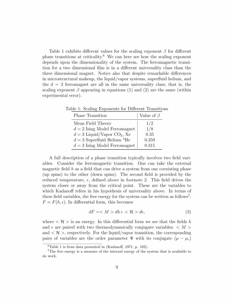
Table 1 exhibits different values for the scaling exponent β for differentphase transitions at criticality.6 We can here see how the scaling exponentdepends upon the dimensionality of the system. The ferromagnetic transi-tion for a two dimensional film is in a different universality class than thethree dimensional magnet. Notice also that despite remarkable differencesin microstructural makeup, the liquid/vapor systems, superfluid helium, andthe d = 3 ferromagnet are all in the same universality class; that is, thescaling exponent β appearing in equations (1) and (2) are the same (withinexperimental error).

Table 1: Scaling Exponents for Different Transitions

Phase Transition Value of β

Mean Field Theory 1/2d = 2 Ising Model Ferromagnet 1/8d = 3 Liquid/Vapor CO2, Xe 0.35d = 3 Superfluid Helium 4He 0.359d = 3 Ising Model Ferromagnet 0.315

A full description of a phase transition typically involves two field vari-ables. Consider the ferromagnetic transition. One can take the externalmagnetic field h as a field that can drive a system from one coexisting phase(up spins) to the other (down spins). The second field is provided by thereduced temperature, ε, defined above in footnote 2. This field drives thesystem closer or away from the critical point. These are the variables towhich Kadanoff refers in his hypothesis of universality above. In terms ofthese field variables, the free energy for the system can be written as follows7:F = F (h, ε). In differential form, this becomes

dF =< M > dh+ < H > dε, (3)

where < H > is an energy. In this differential form we see that the fields hand ε are paired with two thermodynamically conjugate variables: < M >and < H >, respectively. For the liquid/vapor transition, the correspondingpairs of variables are the order parameter Ψ with its conjugate (µ − µc)

6Table 1 is from data presented in (Kadanoff, 1971, p. 102).7The free energy is a measure of the internal energy of the system that is available to

do work.

9

related to the chemical potential. When Kadanoff says that “only the namesof the variables change” for systems in the same universality class these arethe changes to which he refers:

(M,h) ↔ (Ψ, (µ− µc))

The ferromagnetic/paramagnetic phase transition and the liquid/vapor phasetransition are in the same relatively small class.

4.1 Stability

Thus there is a relationship between different phase transitions problems thatleaves invariant various features of those transitions. Here is Kadanoff again:

The theorist can discuss this relation in the following way: Heimagines that yet another field is inserted into the free energy.Call that other field λ and the operator which is its thermo-dynamic conjugate, U . Here λ represents a parameter in theHamiltonian. Continuous variation from λ = 0 to λ = 1 mightrepresent the change in the Hamiltonian which takes us from theIsing model to the Heisenberg model, or from Ni to Fe or froma nearest neighbor interaction to a next nearest neighbor inter-action. Therefore, the discussion of λ and its thermodynamicconjugate U is in effect the discussion of the relationship amongdifferent phase transition problems. (Kadanoff, 1971, p. 105)

Consider the ferromagnetic transition. Inserting this new parameter into theHamiltonian means that the free energy is now a function, not only of themagnetic field h and the field ε, but also of the field λ:

F = F (ε, h, λ).

In differential form we now have

dF =< M > dh+ < H > dε+ < U > dλ. (4)

As an example, consider the Hamiltonian for a nearest neighbor Isingferromagnet:

10

HΩ = −Jn.n.∑<ij>

σiσj − h∑i∈Ω

σi, (5)

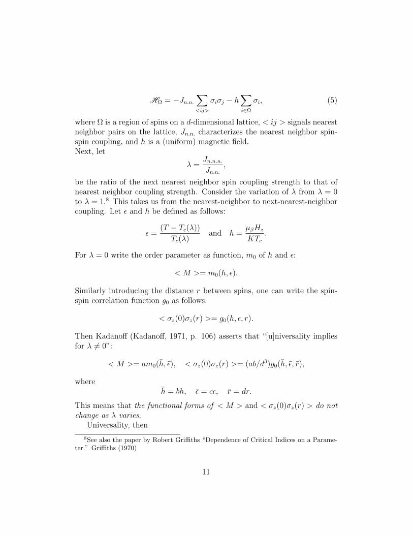
where Ω is a region of spins on a d-dimensional lattice, < ij > signals nearestneighbor pairs on the lattice, Jn.n. characterizes the nearest neighbor spin-spin coupling, and h is a (uniform) magnetic field.Next, let

λ =Jn.n.n.Jn.n.

,

be the ratio of the next nearest neighbor spin coupling strength to that ofnearest neighbor coupling strength. Consider the variation of λ from λ = 0to λ = 1.8 This takes us from the nearest-neighbor to next-nearest-neighborcoupling. Let ε and h be defined as follows:

ε =(T − Tc(λ))

Tc(λ)and h =

µβHz

KTc.

For λ = 0 write the order parameter as function, m0 of h and ε:

< M >= m0(h, ε).

Similarly introducing the distance r between spins, one can write the spin-spin correlation function g0 as follows:

< σz(0)σz(r) >= g0(h, ε, r).

Then Kadanoff (Kadanoff, 1971, p. 106) asserts that “[u]niversality impliesfor λ 6= 0”:

< M >= am0(h, ε), < σz(0)σz(r) >= (ab/d3)g0(h, ε, r),

whereh = bh, ε = cε, r = dr.

This means that the functional forms of < M > and < σz(0)σz(r) > do notchange as λ varies.

Universality, then

8See also the paper by Robert Griffiths “Dependence of Critical Indices on a Parame-ter.” Griffiths (1970)

11

. . . implies that the basic thermodynamic functions and correla-tion functions only depend on λ via a trivial change of variables.The functional form is the same as at λ = 0. However, the vari-ables in these functions are changed in that h, ε, and M areeach multiplied by parameters a, b, c, d which depend upon λ.(Kadanoff, 1971, p. 105)

What does this result mean? It means that the Hamiltonians of differentsystems—as different as9 nickel and iron, or as different as10 CO2, Xe, and4He—can be perturbed into one another without changing the nature of thephase transition problem.11 This, in turn, means that the scaling behavior ofthe order parameter will remain unchanged as the transformation (by varyingthe value of λ) between Hamiltonians is effected. In other words, many ofthe details that genuinely distinguish a lattice of nickel from that of iron(different interatomic strengths, etc.) are irrelevant for the scaling behavior.This is best understood as a stability result. The class of systems representedby their Hamiltonians between which such λ-transformations can take placewithout effecting the scaling behavior of the order parameter (whether it isM , or Ψ, or whatever) is called a “universality class.” It is defined as thatset of systems between which such (perturbative) transformations hold.

This stability under perturbation is the key property of universality. Toexplain how universality is possible, then, requires that one explain two fea-tures:

1. Why are the phase transitions stable under perturbation of the micro-scopic details of the systems (as encoded in their Hamiltonians)?

2. Why are the universality classes dependent12 upon the symmetry of theorder parameter and the dimensionality of the systems13?

9See above quote from Kadanoff.10See Table 1 above.11Not all such transitions will preserve the nature of the phase transition problem. In

fact, a perturbation from an Ising Hamiltonian to a Heisenberg Hamiltonian, will take usfrom one problem to another.

12Recall Kadanoff’s “hypothesis of universality” quoted at the beginning of this section.13It should be clear from the way this question is answered below that the kind of

dependence on symmetry and dimension is not causal. Nor is the explanation of thatdependence causal in nature.

12

“CHAP04” — 2012/9/6 — 17:04 — PAGE 172 — #32

172 the oxford handbook of the philosophy of physics

Figure 4.10 Making blocks. In this illustration a two-dimensional Ising model containing81 spins is broken into blocks, each containing 9 spins. Each one of those blocks is assigneda new spin with a direction set by the average of the old ones. We imagine the model is

reanalyzed in terms of the new spin variables.

result of that calculation and one that might depend upon the exact way in whichwe chose to define the new spin variable.

The equation for the new value of the new deviation from criticality, t =Kc −K ,could be described in similar terms. It is reasonable to assume that if the originalsystem is at its critical point, so is the new description obtained after the blocktransformation. Further it is reasonable to argue that the transformation shouldengender no singularities, thus requiring that a new temperature-deviation fromcriticality would have a linear dependence upon the old deviation. So the remainingpoint is to calculate the coefficient in the linear relation and express it in the specialmanner given in Eq. (18d).

7. The Wilson Revolution. . . . . . . . . . . . . . . . . . . . . . . . . . . . . . . . . . . . . . . . . . . . . . . . . . . . . . . . . . . . . . . . . . . . . . . . . . . . . . . . . . . . . . . . . . . . . . . . . . . .

7.1 Physical Space; Fourier Space

Before entering into Wilson’s construction of the renormalization group theory, Ishould touch upon a point of technique.

The proportionality in Eq. (18d) and Eq. (18c) are representations of scaling,and the coefficients in the linear relations define the scaling relations among thevariables. Note that here scaling is viewed as a change in the effective values of the

Figure 4: Blocking and averaging to yield a new (coarse-grained) effectivesystem (Kadanoff, 2013, p. 172)

5 Explaining Universality

In this section I outline, very briefly, how the renormalization group allows foran explanation of the two key features of universal behavior just mentioned.This explanation has been called into question by a number of commentatorsand I will consider their objections in the following section. Recall the ingre-dients of universality. Near criticality, the correlation length is enormous andthere is a droplets-within-droplets structure that exhibits self-similarity (i.e,it behaves like a fractal). As a result there are no characteristic scales be-tween the atomic/lattice spacing and the continuum. Importantly, as noted,for an infinite system the correlation length actually diverges to infinity.

Kadanoff recognized that one could exploit the droplets-within-dropletsfractal structure to change a Hamiltonian representing a system into a relatedeffective Hamiltonian by a kind of coarse-graining procedure. This is nowknown as the Kadanoff block spin method.

The idea is to group or block spins or molecules and replace them with

13

an some kind of average.14 In figure 4 there are nine spins per block andthe “averaging” rule is to let the majority rule: If more spins in a block areup-spins (down-spins), replace those nine spins with a single “block spin”that points up (down). Now we have a lattice of block spins that lookspretty much like the original lattice but the spacings between the block spinsis greater. Next one spatially rescales so as to put the new spins on thesame lattice as the original. Finally one changes the block spins so that theexhibit coupling strengths as similar to the original coupling as possible.15 Wenow have a new “renormalized” Hamiltonian corresponding to this effectivesystem. Continued iteration of this procedure leads to a flow (the RG flow)on an abstract space of Hamiltonians. That is, it induces a dynamics thattakes one Hamiltonian into another as the blocking procedure is repeated.See figures 5 and 6.

One examines the dynamical flow on this abstract space and looks forpotential fixed points. These are points which when acted upon by thetransformation yield the same point.16 A fixed point is a property of thetransformation itself and all details of the systems that flow toward that fixedpoint have been eliminated. Those systems/models (points in the space)that flow to the same fixed point are in the same universality class—theuniversality class is delimited—and they will exhibit the same macro scalingbehavior.17 That macro-behavior, in particular, the determination of thescaling exponent β in equations (1) and (2) can be determined by an analysisof the transformation in the neighborhood of the fixed point.

Crucially, those systems that actually flow to a fixed point are at criti-cality. This means that they are infinite systems. As such, those systemsare idealizations. But the infinite idealization is necessary if one is to locatethe fixed points of the RG flow in the abstract space. This is because thecorrelation length must diverge to be able to infinitely iterate the RG trans-formation. Nevertheless, systems that are near criticality (real, large finitesystems) will start off close to the critical systems and their behavior can beunderstood by examining the topology of the RG flow in the neighborhood

14It almost doesn’t matter what averaging or coarse-graining scheme is used. This factis just another signature of the stability of phase transitions under perturbation.

15This part of the procedure is to a certain extent an art. There is no explicit recipethat one can follow.

16If τ represents the transformation and p∗ is a fixed point we will have τ(p∗) = p∗.17To put this another way: The universality class is the basin of attraction of the fixed

point.

14

Figure 5: Fixed Point and Universality Class (Fisher 1998, p. 673)

15

Figure 6: Fixed Point, Universality Class, and λ-Transformation

of the fixed point. So, the RG along with the analysis of the topology in theneighborhood of the fixed point provides the explanation of near critical, realsystems.18 It explains what is going on in the neighborhood of the criticalpoint in the boiling region of figure 1.

So the fixed point delimits the class of systems that all exhibit simi-lar behavior near criticality. It also, thereby, justifies the existence of thekind of perturbative stability Kadanoff describes in his discussion of whatwe’ve called the λ-transformations.19 See, figure 6. Finally, this analysisalso demonstrates that the only important or relevant features (other thanbeing near criticality) for this common behavior are the dimensionality ofthe system and the symmetry of the order parameter in the critical region.

18If it only explained the behavior of idealized infinite systems, it would not be sucha big deal. Hardly worthy of a Nobel prize! Note also, contrary to some assertions inthe literature, that the linearization analysis of the flow in the neighborhood of the fixedpoint is not part of the RG. It is a standard technique in dynamical systems theory foranalyzing dynamics near attractor states.

19The justification of the existence of such transformations lies at the heart of the claimthat minimal models like the Ising model need not accurately represent the actual featuresof systems in the universality class.

16

6 Objections and Responses

As noted, a number of philosophers of science have challenged some of theclaims I have just been making. Let me set up my replies to these objec-tions with another quote from Michael Fisher. In “Scaling, Universality,and Renormalization Group Theory” Fisher (1983) expresses what, from acontemporary philosophical perspective, is a rather heretical point of view.

The traditional approach of theoreticians, going back to the foun-dation of quantum mechanics, is to run to Schrodinger’s equationwhen confronted by a problem in atomic, molecular or solid statephysics! One establishes the Hamiltonian, makes some (hope-fully) sensible approximations and then proceeds to attempt tosolve for the energy levels, eigenstates and so on. However, fortruly complicated systems in what, these days, is much bettercalled “condensed matter physics,” this is a hopeless task; fur-thermore, in many ways it is not even a very sensible one!

The modern attitude is, rather, that the task of the theorist isto understand what is going on and to elucidate which are thecrucial features of the problem. For instance, if it is asserted thatthe exponent [β] depends on the dimensionality, d, and on thesymmetry number, n, but on no other factors, then the theorist’sjob is to explain why this is so and subject to what provisos. Ifone had a large enough computer to solve Schrodinger’s equationand the answer came out that way, one would still have no un-derstanding of why this was the case!’ (Fisher, 1983, pp. 46–47)

It is clear from this quote that for Fisher our understanding of universalbehavior requires explaining why the pattern depends upon the dimensionof the system and the symmetry of the order parameter. This, of course, fitsnicely with Kadanoff’s definition of universality (section 4) that explicitlycharacterizes phase transition problems as depending upon the dimensionalityof the system and the symmetries of the order state.

6.1 Objections: Reutlinger and Lange

Alexander Reutlinger holds that the RG explanation for the universal behav-ior of critical phenomena (section 5) proceeds in a completely different, intu-

17

itive, everyday way. He says RG explanations “are not special and quite in-tuitive in one crucial respect. RG explanations explain the phenomenon thatmicroscopically different physical systems display the same macro-behavior. . . by referring to features that those physical systems have in common, al-though the physical systems at issue are different in many other respects.”(Reutlinger, 2017, p. 144) The “common features” that are supposed toexplain the universal behavior are the common dimensionality and the com-mon symmetry of the order parameters. To cite these features, accordingto Ruetlinger, just is to explain the universal critical behavior of fluids andmagnets.

In a reply to a paper by Collin Rice and me, Lange (2015) argues similarlyfor what Ruetlinger calls the “commonality strategy.” He holds that ourjustification of why minimal models like the Ising model can be used tounderstand the behaviors of actual systems also depends upon citing commonfeatures. He asserts that “since the model’s explanatory utility arises fromits having certain features in common with the target system, the model’sexplanatory utility arises from its representing accurately enough the targetsystem, contrary to B&R’s [Batterman’s and Rice’s] view.” (Lange, 2015,p. 298) Specifically, the claim is that a minimal or “toy” model can beexplanatory if it shares features (dimension and symmetry in the case of theIsing model) with the actual target, fluid system.

In our paper, Rice and I argue that the justification for the applica-bility of minimal models derives from the demonstration that the minimalmodel is in the same universality class as the target system of interest. Thediscussion above aims in part to show how the RG demonstrates this veryfact. Furthermore, and importantly, we have seen that this demonstrationalso provides an account of why dimensionality and symmetry are importantfeatures characteristic of the universality class.

But Lange asks why do “B&R insist that a minimal model explanationmust explain why the common features are necessary for the macrobehaviorto occur and why these features are present in all members of the universal-ity class despite their heterogeneous microdetails?” (Lange, 2015, p. 303)The answer to these questions, once one properly understands what it is tobe a universality class, is that one needs to show that those very features(symmetry and dimensionality) are the important common features. Thisfits with the above discussion of the definition of universality (section 4) andwith the insistence by Fisher (in the quote above) that “the theorist’s job isto explain why [the common exponent β depends upon the dimensionality d

18

and the symmetry number n]. (Fisher, 1983, pp. 47)Lange does appeal to a passage from Fisher that comes just after the one

quoted above:

We may well try to simplify the nature of a model to the pointwhere it represents a ‘mere caricature’ of reality. But notice thatwhen one looks at a good political cartoon one can recognize thevarious characters even though the artist has portrayed them withbut a few strokes. . . . [A] good theoretical model of a complexsystem should be like a good caricature: it should emphasizethose features which are most important and should downplaythe inessential details.” (Fisher, 1983, p. 47)

Lange claims that here Fisher “seems to be supporting a ‘common featuresaccount’: the minimal model, despite being a caricature of some actual sys-tem, shares with it ‘those features which are most important.’ ”(Lange, 2015,p. 299, fn. 3)

Of course Lange is right about this. But the question is why are those thefeatures that are important! Without an answer to that question, we neitherhave a justification for the use of the minimal model, nor an explanation ofuniversal behavior.

6.2 Objections: Franklin and Mainwoood

Alexander Franklin has recently argued that the Kadanoff blocking scheme(aka “real”-space RG) discussed above, cannot explain the possibility of uni-versal behavior. Franklin (2017) He says that

[b]uilding on Mainwood (2006) I argue that the [real-space RGand the field-theoretic RG] approaches ought to be distinguished:while the field-theoretic approach explains universality, the real-space approach fails to provide an adequate explanation. (Franklin,2017, p.1)

Without going into too much detail, I want to argue that this claim is mis-taken. The error is two-fold. First, the claim rests on a mistaken characteri-zation of universality (similar to the view held by of Reutlinger and Lange).On this mistaken view, one fails to realize that to explain universality (as I’vediscussed above) requires that one explain the dependence of the macropat-tern on the symmetry and dimension. Second, Franklin’s assertion rests upon

19

a myth (whose genesis in philosophical discussions, I believe, is Mainwood’sdissertation Mainwood (2006)); namely, that there really are two kinds ofRG explanations, one given by the real-space (or Kadanoff) approach, theother by a so-called field-theoretic (or Wilsonian) approach.

We have seen above how the real-space approach is supposed to work.And, it is true that physics textbooks often do refer to the field-theoreticapproach as distinct. In fact, one text upon which Franklin relies makes thedistinction between the two types of RG explanations quite explicit. Binneyet al. (1992) I think this distinction (between real-space and field-theoreticRG) makes some sense and does simplify some calculations. However, itbegs the important question when it comes to explaining universality. Thatis, the so-called “field-theoretic” approach assumes universality rather thanexplaining it.

The field-theoretic “explanation” starts with what is known as the Landau-Ginzburg-Wilson (LGW) Hamiltonian:

H =

∫ddx

[1

2ζ2|∇φ(x)|2 +

1

2θ|φ(x)|2 +

1

4!η|φ(x)|4

]. (6)

For my purposes here it suffices to note two features of this Hamilto-nian (neither of which is controversial). First, φ(x) is an order parameter(like Ψ or M) and that, within the LGW Hamiltonian, only even powers ofthat order parameter appear. Second, the LGW Hamiltonian is an effectiveHamiltonian. This latter feature means that the LGW Hamiltonian is not amicroscopic characterization of the system. In fact, since it makes referenceto the order parameter φ(x), given the discussion in section 3 it is a mesoscaleHamiltonian. Thus, unlike the real-space RG explanation that starts withmicroscopic Hamiltonians, the field-theoretic approach begins with a Hamil-tonian that already ignores various microscopic details that distinguish dif-ferent systems. Most importantly, the LGW Hamiltonian’s elimination ofodd power terms of the order parameter, is a reflection of the symmetry ofthat order parameter.

In other words, the LGW Hamiltonian is designed to represent systemsthat share the same dimensionality and order parameter symmetry. There-fore, it cannot (on pain of circularity) serve to explain why the systems in theuniversality class have those properties as common features. It is surely truethat condensed matter physicists often start with the effective (mesoscopic)LGW Hamiltonian, rather than a more realistic (or at least more detailed),

20

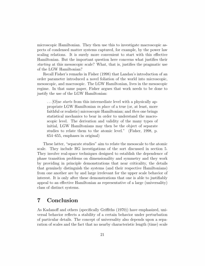
microscopic Hamiltonian. They then use this to investigate macroscopic as-pects of condensed matter systems captured, for example, by the power lawscaling relations. It is surely more convenient to start with this effectiveHamiltonian. But the important question here concerns what justifies theirstarting at this mesoscopic scale? What, that is, justifies the pragmatic useof the LGW Hamiltonian?

Recall Fisher’s remarks in Fisher (1998) that Landau’s introduction of anorder parameter introduced a novel foliation of the world into microscopic,mesoscopic, and macrosopic. The LGW Hamiltonian, lives in the mesoscopicregime. In that same paper, Fisher argues that work needs to be done tojustify the use of the LGW Hamiltonian:

. . . [O]ne starts from this intermediate level with a physically ap-propriate LGW Hamiltonian in place of a true (or, at least, morefaithful or realistic) microscopic Hamiltonian; and then one bringsstatistical mechanics to bear in order to understand the macro-scopic level. The derivation and validity of the many types ofinitial, LGW Hamiltonians may then be the object of separatestudies to relate them to the atomic level.” (Fisher, 1998, p.654–655, emphases in original)

These latter, “separate studies” aim to relate the mesoscale to the atomicscale. They include RG investigations of the sort discussed in section 5.They involve real-space techniques designed to establish the dependence ofphase transition problems on dimensionality and symmetry and they workby providing in principle demonstrations that near criticality, the detailsthat genuinely distinguish the systems (and their respective Hamiltonians)from one another are by and large irrelevant for the upper scale behavior ofinterest. It is only after these demonstrations that one is able to justifiablyappeal to an effective Hamiltonian as representative of a large (universality)class of distinct systems.

7 Conclusion

As Kadanoff and others (specifically Griffiths (1970)) have emphasized, uni-versal behavior reflects a stability of a certain behavior under perturbationof particular details. The concept of universality also depends upon a sepa-ration of scales and the fact that no nearby characteristic length (time) scale

21

is present. Finally, it is part of the very concept of universality of criticalphenomena that the (universality) class of systems depends upon the dimen-sionality of the system and the symmetry of the ordered state. Thus, anyexplanation for how the universality of critical phenomena can be possiblerequires demonstrations that the systems are stable under the appropriate(λ-)perturbation and that the only system features relevant to the behaviorare the physical dimensionality and the symmetry of the ordered state.

The renormalization group can provide these two demonstrations. It doesso by introducing a transformation on an abstract space of Hamiltonianscorresponding to actual and possible systems and finding fixed points ofthat transformation. The Hamiltonians that flow to the same fixed pointare exactly those between which the perturbative (λ) stability holds. Theyare also those critical systems that share dimensionality and the appropriatemeso-scale symmetry.

As discussed in section 6 a number of objections have been offered tothis RG explanation. I answer these by looking back at the historical dis-cussions in which the concept “universality” first appeared as an expres-sion of similar behavior by radically distinct systems. The arguments abovedemonstrate that the the commonality strategy for explaining universalityjust won’t work. In fact, since universality is a statement to the effect thatthe similar behaviors of critical systems depend only on dimensionality andsymmetry, to explain how universal behavior is possible requires explain-ing the dependence upon dimensionality and symmetry. Simply citing thoseproperties as explanans is just to cite part of the explanandum, and hence,provides no explanation at all. Finally, appealing to a field-theoretic RGthat starts with an effective Hamiltonian fails to meet the explanatory task.The effective (LGW) Hamiltonian requires justification. As it is effective, itactually expresses the very universality one seeks to explain.

22

References

Batterman, Robert W. 2002a. Asymptotics and the role of minimal models.The British Journal for the Philosophy of Science, 53:21–38, 2002a.

Batterman, Robert W. 2002b. The Devil in the Details: Asymptotic Reason-ing in Explanation, Reduction, and Emergence. Oxford Studies in Philos-ophy of Science. Oxford University Press.

Batterman, Robert W. 2018. Multiscale modeling in inactive and activematerials. Unpublished.

Binney, J. J., N. J. Dowrick, A. J. Fisher, and M. E. J. Newman. 1992. TheTheory of Critical Phenomena: An Introduction to the RenormalizationGroup. Oxford University Press.

Fisher, Michael E. 1983. Scaling, universality and renormalization group the-ory. In F.J.W. Hahne, editor, Critical Phenomena, volume 186 of LectureNotes in Physics, Berlin, 1983. Summer School held at the University ofStellenbosch, South Africa; January 18–29, 1982, Springer-Verlag.

Fisher, Michael E. 1998. Renormalization group theory: Its basis and formu-lation in statistical physics. Reviews of Modern Physics, 70(2):653–681.

Franklin, Alexander. 2018. On the renormalisation group explanation ofuniversality. Philosophy of Science DOI: 10.1086/696812.

Grifiths, Robert B. 1970. Dependence of critical indices on a parameter.Physical Review Letters, 24(26):1479–1482.

Guggenheim, E. A. 1945. The principle of corresponding states. The Journalof Chemical Physics, 13(7):253–261.

Kadanoff, Leo P. 1971. Critical Behavior. Universality and Scaling. In M. S.Green, editor, Proceedings of the International School of Physics “EnricoFermi” Course LI, volume Course LI, pages 100–117, New York. ItalianPhysical Society, Academic Press.

Kadanoff, Leo P. 1976. Scaling, universality, and operator algebras. InC. Domb and M. S. Green, editors, Phase Transitions and Critical Phe-nomena, volume 5A. Academic Press.

23

Kadanoff, Leo P. 2000. Statistical Physics: Statics, Dynamics, and Renor-malization. World Scientific, Singapore.

Kadanoff, Leo P. 2013 Theories of matter: Infinities and renormalization.In Robert W. Batterman, editor, The Oxford Handbook of Philosophy ofPhysics, chapter Four, pages 141–188. Oxford University Press.

Landau, L. D. 1965. On the theory of phase transistions. In D. Ter Haar, ed-itor, Collected Papers of L. D. Landau, chapter 29, pages 193–216. Gordonand Breach, Science Publishers, New York.

Lange, Marc. 2015. On “minimal model explanations”: A reply to battermanand rice. Philosophy of Science, 82:292–305.

Mainwood, Paul. 2006. Is More Different? Emergent Properties in Physics.PhD thesis, Merton College, University of Oxford.

Reutlinger, Alexander. 2017. Do renormalization group explanations conformto the commonality strategy? Journal of General Philosophy of Science,48:143–150.

24