Universal Properties of

Poker TournamentsPersistence, the “leader problem”

and extreme value statistics

Clément SireLaboratoire de Physique Théorique

CNRS & Université Paul Sabatier

Toulouse, France

www.lpt.ups-tlse.fr

Introduction

Statistical physicists are more and more interested in systems out of the realm of physics (networks, competitive systems, epidemics, finance, biology…)

Poker tournaments are perfectly isolated systems, a priori obeying purely “human” laws (bluff, prudence, aggressiveness…)

Link with other physics/probability problems: persistence, the “leader problem”, extreme value statistics

The “Science” of Poker

Head-to-head game “La Relance” introduced by Émile Borel (1938):

Player A and B put 1$ in the pot and are each distributed a hand of value c2[0,1]; A starts:

Borel obtained the best strategy for A and B

A starts

A raises R$ if cA>rA

B calls R$

if cB>rB

Best hand wins (R+1)$

B folds

if cB<rB

A wins 1$

A folds

if cA<rA

B wins 1$

The “Science” of Poker

John von Neumann (1944) modifies the rules of “La Relance” to include bluff

Player A and B put 1$ in the pot and are each distributed a hand of value c2[0,1]; A starts:

The best A-strategy now involves random bluffing

A starts

A raises R$

if cA>rA or if cA<sA

B folds A wins 1$

B calls R$

if cB>rB

Best hand wins (R+1)$

A checks

if sA<cA<rA

Best hand wins 1$

The “Science” of Poker

Strategies for more complicated/realistic rules for head-to-head poker haven been obtained

“Poker bots” now learn to adapt and mixtheir strategies (two-player game)

Poker bots in multiplayer games are still bad

In this work, we are interested in the overall statistical properties of poker tournaments (strategies are irrelevant)

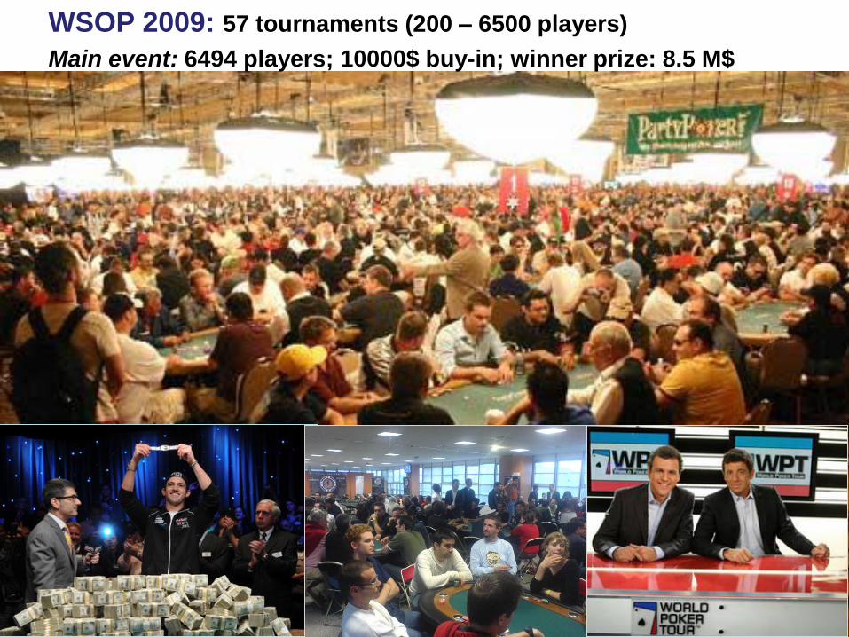
WSOP 2009: 57 tournaments (200 – 6500 players)

Main event: 6494 players; 10000$ buy-in; winner prize: 8.5 M$

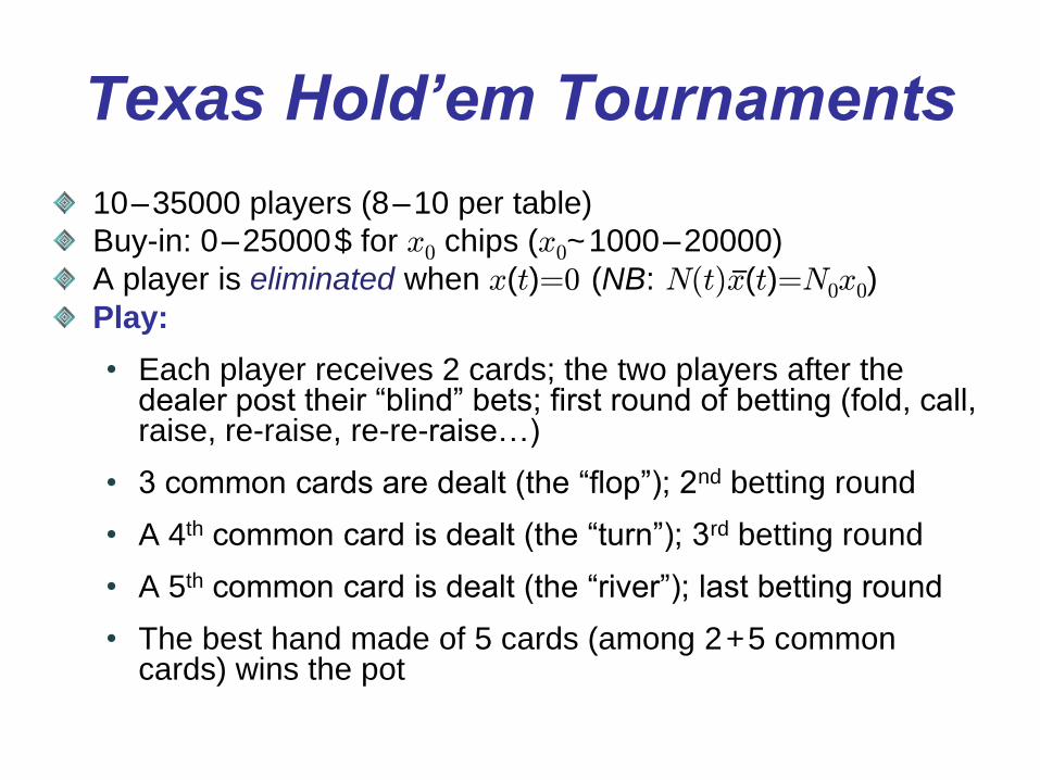
Texas Hold’em Tournaments

10–35000 players (8–10 per table)

Buy-in: 0–25000$ for x0 chips (x0~1000–20000)

A player is eliminated when x(t)=0 (NB: N(t)x(t)=N0x0)

Play:

• Each player receives 2 cards; the two players after the dealer post their “blind” bets; first round of betting (fold, call, raise, re-raise, re-re-raise…)

• 3 common cards are dealt (the “flop”); 2nd betting round

• A 4th common card is dealt (the “turn”); 3rd betting round

• A 5th common card is dealt (the “river”); last betting round

• The best hand made of 5 cards (among 2+5 common cards) wins the pot

–

Example of Texas Hold’em Play

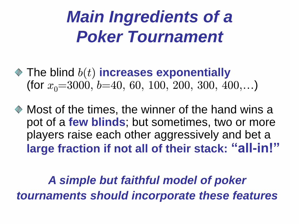
Main Ingredients of a

Poker Tournament

The blind b(t) increases exponentially(for x0=3000, b=40, 60, 100, 200, 300, 400,…)

Most of the times, the winner of the hand wins a pot of a few blinds; but sometimes, two or more players raise each other aggressively and bet a

large fraction if not all of their stack: “all-in!”

A simple but faithful model of poker

tournaments should incorporate these features

A Model of Poker Tournaments

N0 players distributed on tables of T=10 seats receive x0chips

At the start of any deal, the “blinder” posts the blind b(t)=b0exp(t/t0) (x0Àb0)

Each player receives a hand (a random number c[0;1])

Players can call (i.e. bet b) with probability p(c), if c<1-q, go all-in, if c>1-q (and can be called by other players having a hand c>1-q), and fold otherwise NB: p(c) is irrelevant; for instance, p(c)=cn

The best hand wins the pot; time is updated to t+1

Tables run in parallel; players are redistributed on empty seats in order to minimize the number of active tables

Poker Model without All-in (q=0)

The stack x(t) of an individual player is a generalized random walker:

x(t+1)=x(t)+b(t)(t)

where t is the number of hands played, and

→ h(t)i=0 (no winning strategy/chips are conserved)

→ h(t)(t’)i=t,t’2 (successive deals are uncorrelated)

The considered player is eliminated when x(t)=0

The number P(x,t) of players still in game with a stack x obeys the Fokker-Planck equation:

with the absorbing boundary condition P(x=0,t)=0

Link to the persistence problem

Physical Applications of Persistence

Persistence exponent of the Ising model: local and global persistence; a new critical exponent for lattice spin systems

Persistence exponent for the diffusion equation

Persistence for any level M: distribution of the minima and maximaof a process,

Many other experimental measurements (breath figures, Si surfaces, soap bubbles, rare gas…)

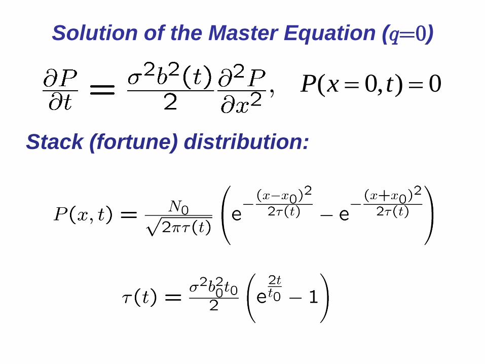
Solution of the Master Equation (q=0)

Stack (fortune) distribution:

( 0, ) 0P x t ,

Scaling Regime (q=0)

Stack distribution:

Exponential decay of the number of players controlled by the growth rate of the blind:

Universal scaling function:

Estimate of the duration of a tournament:

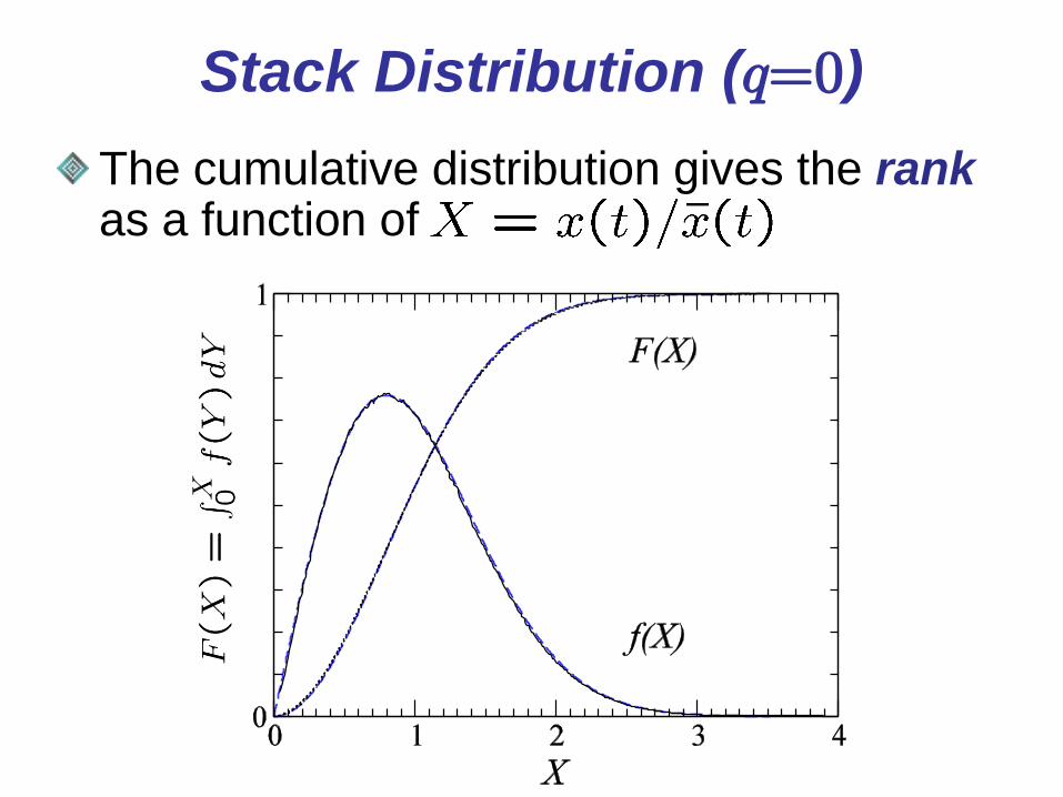
Stack Distribution (q=0)

The cumulative distribution gives the rankas a function of

All-in Decay Rate

Probability of an all-in event at a given table (q¿1):

Population decay due to all-in events:

The Optimal All-in Probability

If , the tournament is dominated by all-in events (players are taking stupid risks just to win the blind)

If , the players (especially those with small stacks) do not take enough the opportunity to double their stack with a very good hand

The optimal q is such that

All-in Kernel (time argument dropped):

All-in decay rate:

Master Equation Including All-in Events

à Wins against a bigger stack

à Wins and eliminates a poorer

player

à Looses but survives against a

poorer player

Scaling stack distribution:

Scaling equation (integro-differential and non-linear; no parameter):

Scaling Equation

Internet Tournaments (22-55$ buy-in)

WPT 2006 data (10000$ buy-in)

Properties of the “Chip Leader”

The number of successive “chip leaders” growths logarithmically with the number of initial players

The “Leader Problem”

Competing agents get a time-dependent “score”

where s is any continuous increasing function (arises in evolutionary biology)

The fitnesses vi are independently drawn from the same distribution f(v)

Then, the average total number of leaders and its variance verify:

where the constants ¯ and ° are universal and only depend on the large v properties of f(v) (3 universality classes)

Ref.: C. Sire, S.N. Majumdar, and D.S. Dean, J. Stat. Mech., L07001 (2006) ; reprint on arxiv.org/abs/cond-mat/0606101

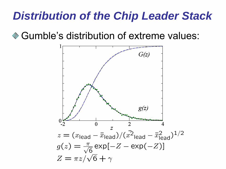
Distribution of the Chip Leader Stack

Gumble’s distribution of extreme values:

Conclusion

Successful modeling of poker tournaments after identifying their two main properties (exponential growth of the blind, all-in events) and the irrelevance of individual strategies

Link to persistence, the “leader problem”, and extreme value statistics

Refs: C. Sire, J. Stat. Mech. P08013 (2007); reprint onarXiv/physics/0703122

Articles in the Scientific American, the New Scientist, PhysOrg.com, Poker Live Magazine, Libération, BBC Focus, and hundreds of poker web sites…

Other recent game theory applications: contest on a random polymer, baseball and football championships…

Persistence of a non-Markovian

stationary Gaussian random walker

A stationary Gaussian random walker x(¿) is fully characterized by f(¿)=hx(¿)x(0)i

The persistence is the probability that x(s) remains above (or below) a certain level M, for all s2[0,¿]; P(¿)»exp(-µ¿)

f(¿)=exp(-¸¿) means that x(¿) is Markovian

If hy(t)y(t’)i=g(t/t’), then x(¿)=y(exp ¿) is stationary in the new variable ¿=ln t; hence, P(t)»t-µ

Many physical quantities of interest are Gaussian or well approximated by a Gaussian process

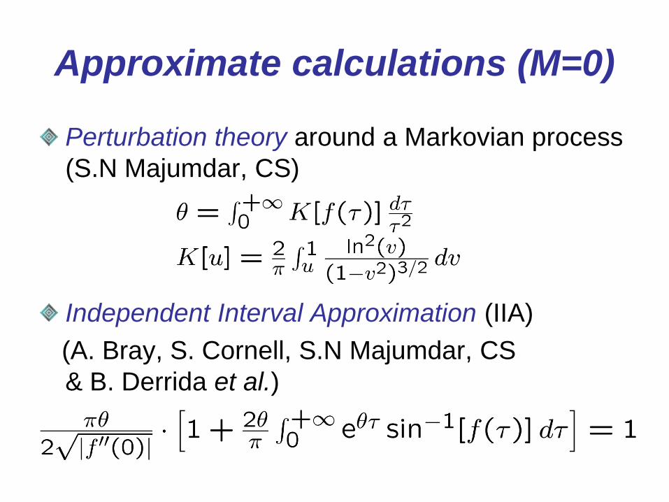
Approximate calculations (M=0)

Perturbation theory around a Markovian process

(S.N Majumdar, CS)

Independent Interval Approximation (IIA)

(A. Bray, S. Cornell, S.N Majumdar, CS

& B. Derrida et al.)

Physical applications

Persistence exponent of the Ising model: local and global persistence (PT); a new critical exponent for lattice spin systems

Persistence exponent for the diffusion equation

Persistence for any level M (CS): distribution of the minima and maxima of a Gaussian process,

Many other experimental measurements (breath figures, Sisurfaces, soap bubbles, rare gas…)

References

Perturbation theory:

- S.N. Majumdar, C. Sire, Phys. Rev. Lett. 77,1420 (1996); reprint on arXiv:cond-mat/9604151

- S.N. Majumdar, A.J. Bray, S.J. Cornell, C. Sire, Phys. Rev. Lett. 77, 3704 (1996); reprint on arXiv:cond-mat/9606123

- C. Sire, S.N. Majumdar, A. Rüdinger, Phys. Rev. E 61, 1258 (2000); reprint on arXiv:cond-mat/9810136

Independent Interval Approximation:

- S.N. Majumdar, A.J. Bray, S.J. Cornell, C. Sire, Phys. Rev. Lett. 77, 2867 (1996); reprint on arXiv:cond-mat/9605084

- B. Derrida, V. Hakim, R. Zeitac, Phys. Rev. Lett. 77, 2871 (1996); reprint on arXiv:cond-mat/9606005

Distribution of the extrema of a smooth Gaussian walker:

- C. Sire, Phys. Rev. Lett. 98, 020601 (2007); reprint on arXiv:cond-mat/0606145

Other competitive systems:

baseball and soccer (CS & S. Redner)

Fraction of wins vs rank during the two major baseball

eras (1900-1960; 1961-2007) & the corresponding

streaks pdf (one parameter model)

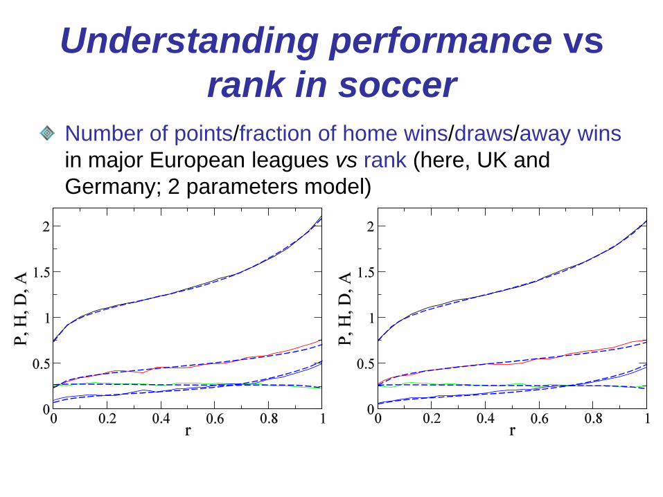
Understanding performance vs

rank in soccer

Number of points/fraction of home wins/draws/away wins

in major European leagues vs rank (here, UK and

Germany; 2 parameters model)