Unit V Relational Algebra - gfgc.kar.nic.in
12
1 Unit V Relational Algebra and Relational Calculus Relational Algebra: Relational algebra is a collection of operations that are used to manipulate the entire set of relations. The output of any relational algebra operation is always a relation. A sequence of relational algebra operations forms a relational algebra expression, whose result will also be a relation that represents the result of a database query. The relational algebra is often considered to be an integral part of the relational data model. Its operations can be divided into two groups. 1. SELECT, PROJECT, and JOIN. 2. Set Operations: UNION, INTERSECTION, SET DIFFERENCE, CARTESIAN PRODUCT. Let us consider the following tables which will be used to demonstrate the SELECT and PROJECT operations. EMPLOYEE SSN Name DOB Address Gender Salary SuperSSN DNo 1111 Divya 20-Feb-82 Malleswaram M 22000 4444 1 2222 Scott 10-Dec-60 Rajajinagar M 30000 4444 3 3333 Pooja 22-Jan-65 Indiranagar F 18000 2222 2 4444 Prasad 11-Jan-57 Rajajinagar M 32000 Null 3 5555 Reena 15-Jan-85 MG Road F 8000 4444 3 PROJECTS PNo PName PLocation DNo 10 Library Management USA 2 20 ERP Chennai 1 30 Hospital Management Mumbai 3 40 Wireless Network London 2 The SELECT Operation (σ): The SELECT operation is used to select a subset of the tuples from a relation that satisfies a selection condition. The SELECT operation can also be visualized as a horizontal partition of the relation into two sets of tuples. One set of tuples that satisfy the condition and are selected, another set of tuples that do not satisfy the condition and discarded. This particular operation allows us to manipulate data in single relation. It uses a mathematical symbol, σ (sigma) and name of the relation is shown in brackets and the condition as a subscript. The general form of selection operation is shown below. σ <selection-condition> (Relation) The <selection-condition> in the above syntax may contain logical and arithmetic operators. Relation is the name of the relation from which the data will be selected. We can use operators such as =, <, <=, >=, >, ≠, etc. and also Boolean operators like and, or, and not.
Transcript of Unit V Relational Algebra - gfgc.kar.nic.in
1
Unit V
Relational Algebra and Relational Calculus
Relational Algebra:
Relational algebra is a collection of operations that are used to manipulate the entire set of
relations. The output of any relational algebra operation is always a relation. A sequence of
relational algebra operations forms a relational algebra expression, whose result will also be a
relation that represents the result of a database query.
The relational algebra is often considered to be an integral part of the relational data model. Its
operations can be divided into two groups.
1. SELECT, PROJECT, and JOIN.
2. Set Operations: UNION, INTERSECTION, SET DIFFERENCE, CARTESIAN PRODUCT.
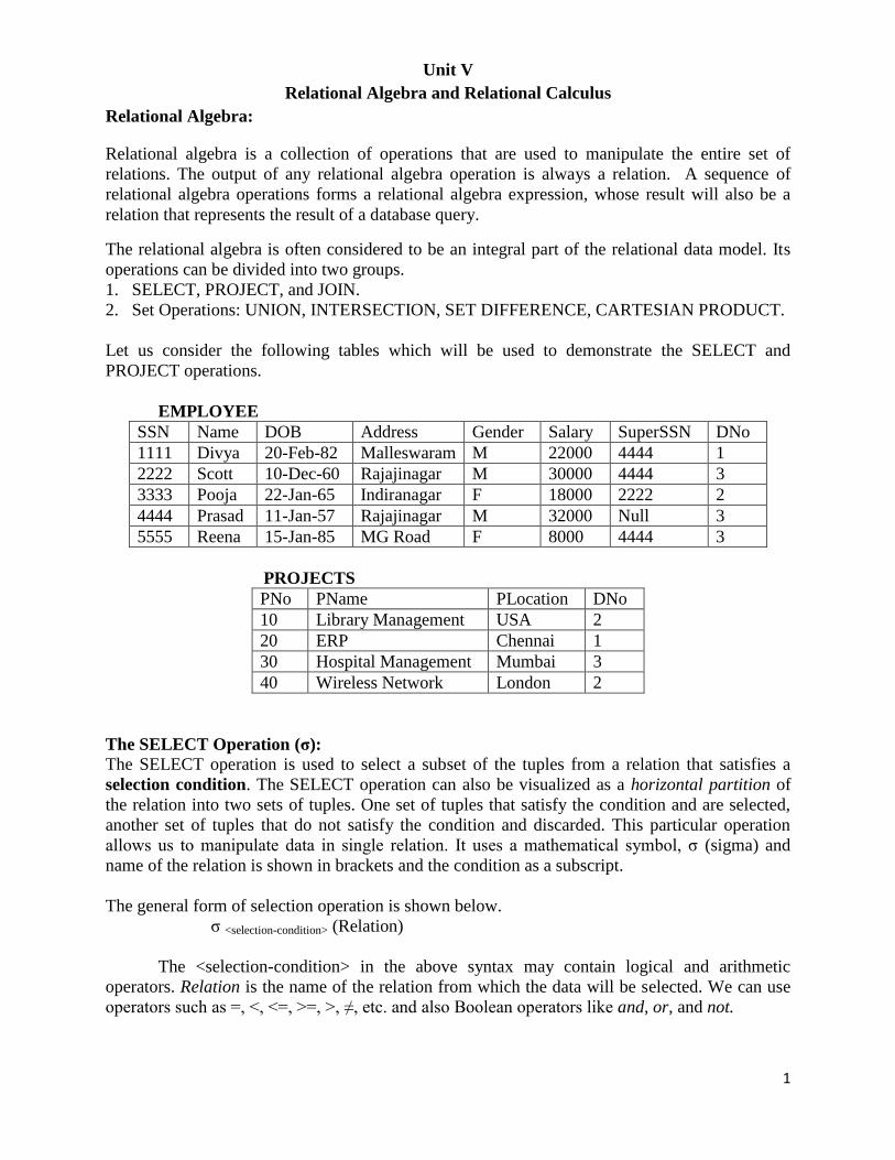
Let us consider the following tables which will be used to demonstrate the SELECT and
PROJECT operations.
EMPLOYEE
SSN Name DOB Address Gender Salary SuperSSN DNo
1111 Divya 20-Feb-82 Malleswaram M 22000 4444 1
2222 Scott 10-Dec-60 Rajajinagar M 30000 4444 3
3333 Pooja 22-Jan-65 Indiranagar F 18000 2222 2
4444 Prasad 11-Jan-57 Rajajinagar M 32000 Null 3
5555 Reena 15-Jan-85 MG Road F 8000 4444 3
PROJECTS
PNo PName PLocation DNo
10 Library Management USA 2
20 ERP Chennai 1
30 Hospital Management Mumbai 3
40 Wireless Network London 2
The SELECT Operation (σ):
The SELECT operation is used to select a subset of the tuples from a relation that satisfies a
selection condition. The SELECT operation can also be visualized as a horizontal partition of
the relation into two sets of tuples. One set of tuples that satisfy the condition and are selected,
another set of tuples that do not satisfy the condition and discarded. This particular operation
allows us to manipulate data in single relation. It uses a mathematical symbol, σ (sigma) and
name of the relation is shown in brackets and the condition as a subscript.
The general form of selection operation is shown below.
σ <selection-condition> (Relation)
The <selection-condition> in the above syntax may contain logical and arithmetic
operators. Relation is the name of the relation from which the data will be selected. We can use
operators such as =, <, <=, >=, >, ≠, etc. and also Boolean operators like and, or, and not.
2
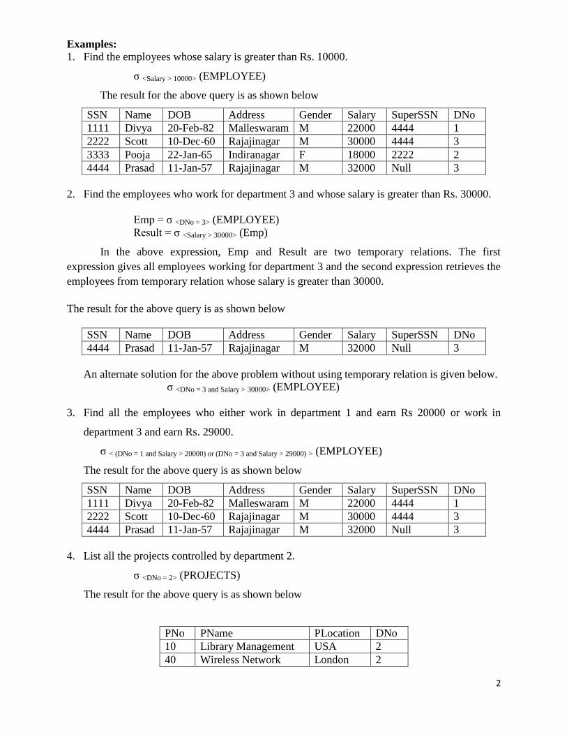
Examples:
1. Find the employees whose salary is greater than Rs. 10000.
σ <Salary > 10000> (EMPLOYEE)
The result for the above query is as shown below
SSN Name DOB Address Gender Salary SuperSSN DNo
1111 Divya 20-Feb-82 Malleswaram M 22000 4444 1
2222 Scott 10-Dec-60 Rajajinagar M 30000 4444 3
3333 Pooja 22-Jan-65 Indiranagar F 18000 2222 2
4444 Prasad 11-Jan-57 Rajajinagar M 32000 Null 3
2. Find the employees who work for department 3 and whose salary is greater than Rs. 30000.
Emp = σ <DNo = 3> (EMPLOYEE)
Result = σ <Salary > 30000> (Emp)
In the above expression, Emp and Result are two temporary relations. The first
expression gives all employees working for department 3 and the second expression retrieves the
employees from temporary relation whose salary is greater than 30000.
The result for the above query is as shown below
SSN Name DOB Address Gender Salary SuperSSN DNo
4444 Prasad 11-Jan-57 Rajajinagar M 32000 Null 3
An alternate solution for the above problem without using temporary relation is given below.
σ <DNo = 3 and Salary > 30000> (EMPLOYEE)
3. Find all the employees who either work in department 1 and earn Rs 20000 or work in
department 3 and earn Rs. 29000.
σ < (DNo = 1 and Salary > 20000) or (DNo = 3 and Salary > 29000) > (EMPLOYEE)
The result for the above query is as shown below
SSN Name DOB Address Gender Salary SuperSSN DNo
1111 Divya 20-Feb-82 Malleswaram M 22000 4444 1
2222 Scott 10-Dec-60 Rajajinagar M 30000 4444 3
4444 Prasad 11-Jan-57 Rajajinagar M 32000 Null 3
4. List all the projects controlled by department 2.
σ <DNo = 2> (PROJECTS)
The result for the above query is as shown below
PNo PName PLocation DNo
10 Library Management USA 2
40 Wireless Network London 2
3
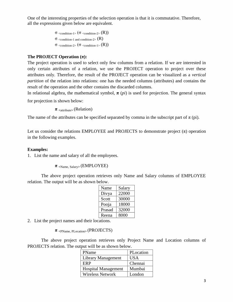
One of the interesting properties of the selection operation is that it is commutative. Therefore,
all the expressions given below are equivalent.
σ <condition-1> (σ <condition-2> (R))
σ <condition-1 and condition-2> (R)
σ <condition-2> (σ <condition-1> (R))
The PROJECT Operation (π):
The project operation is used to select only few columns from a relation. If we are interested in
only certain attributes of a relation, we use the PROJECT operation to project over these
attributes only. Therefore, the result of the PROJECT operation can be visualized as a vertical
partition of the relation into relations: one has the needed columns (attributes) and contains the
result of the operation and the other contains the discarded columns.
In relational algebra, the mathematical symbol, π (pi) is used for projection. The general syntax
for projection is shown below:
π <attribute> (Relation)
The name of the attributes can be specified separated by comma in the subscript part of π (pi).
Let us consider the relations EMPLOYEE and PROJECTS to demonstrate project (π) operation
in the following examples.
Examples:
1. List the name and salary of all the employees.
π <Name, Salary> (EMPLOYEE)
The above project operation retrieves only Name and Salary columns of EMPLOYEE
relation. The output will be as shown below.
Name Salary
Divya 22000
Scott 30000
Pooja 18000
Prasad 32000
Reena 8000
2. List the project names and their locations.
π <PName, PLocation> (PROJECTS)
The above project operation retrieves only Project Name and Location columns of
PROJECTS relation. The output will be as shown below.
PName PLocation
Library Management USA
ERP Chennai
Hospital Management Mumbai
Wireless Network London

4
3. Retrieve the Name and Salary of all employees who are working for department 1.
π <Name, Salary> (σ <DNo=1> (EMPLOYEE))
The above query involves two operations, First, SELECT operation is applied to retrieve
the employees who are working in department 1 and it gives entire tuples which satisfies the
condition. Second, we have to retrieve only name and salary of the employees from the first
operation.
Name Salary
Divya 22000
Alternatively, we can split the above query into two queries by making use of intermediate
relations.
Dept1 = σ <DNo=1> (EMPLOYEE)
Dept1
SSN Name DOB Address Gender Salary SuperSSN DNo
1111 Divya 20-Feb-82 Malleswaram M 22000 4444 1
Result = π <Name, Salary> (Dept1)
Result
Name Salary
Divya 22000
4. Find the name, address, and salary of the employees who earn more than 25,000 rupees.
π <Name, Salary, Address> (σ <Salary > 25000> (EMPLOYEE))
The result of the above query is,
Name Address Salary
Scott Rajajinagar 30000
Prasad Rajajinagar 32000
5. List the name and location of the projects which are not controlled by department 2.
π <PName, PLocation> (σ <DNo ≠ 2> (PROJECTS))
PName PLocation
ERP Chennai
Hospital Management Mumbai

5
RENAME (ρ) Operation:
In general, we may want to apply several relational algebra operations one after the other. In
such case we may want to rename the relation name or attribute name or both relation name and
attribute name. This is done with the help special operation which is use to perform the renaming
operation. It is a unary operator.
The general RENAME operation when applied to a relation R of degree n is denoted by any of
the following three forms:
ρ S(B1, B2, … Bn)(R) or ρS(R) or ρ(B1, B2, … Bn)(R)
Where the ρ (rho) is used to denote the RENAME operator, S is the new relation name, and B1,
B2, … Bn are the new attribute names. The first expression renames both the relation and its
attributes, the second renames the relation only, and the third renames the attributes only.
Let us consider an EMPLOYEE relation to rename the attributes and giving new name to result
relation.
TEMP ← σ<Dno=5>(EMPLOYEE)
R(First_name, Last_name, Salary) ← π<Fname, Lname, Salary>(TEMP)
6
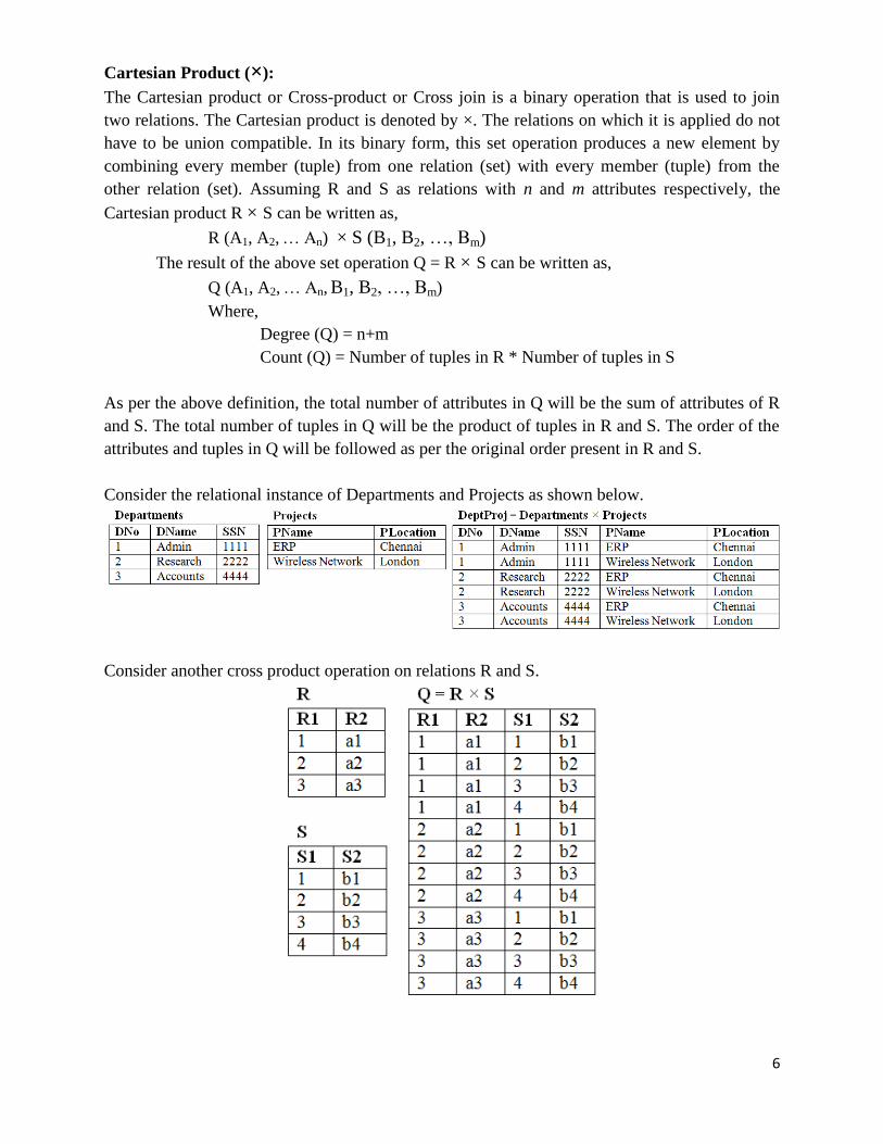
Cartesian Product (×):
The Cartesian product or Cross-product or Cross join is a binary operation that is used to join
two relations. The Cartesian product is denoted by ×. The relations on which it is applied do not
have to be union compatible. In its binary form, this set operation produces a new element by
combining every member (tuple) from one relation (set) with every member (tuple) from the
other relation (set). Assuming R and S as relations with n and m attributes respectively, the
Cartesian product R × S can be written as,
R (A1, A2, … An) × S (B1, B2, …, Bm)
The result of the above set operation Q = R × S can be written as,
Q (A1, A2, … An, B1, B2, …, Bm)
Where,
Degree (Q) = n+m
Count (Q) = Number of tuples in R * Number of tuples in S
As per the above definition, the total number of attributes in Q will be the sum of attributes of R
and S. The total number of tuples in Q will be the product of tuples in R and S. The order of the
attributes and tuples in Q will be followed as per the original order present in R and S.
Consider the relational instance of Departments and Projects as shown below.
Consider another cross product operation on relations R and S.
7
JOIN Operations:
Join is used to fetch data from two or more tables, which is joined to appear as single set of data.
It is used for combining column from two or more tables by using values common to both tables.
Different types of joins:
1. Inner Join
a. Natural Join
b. Theta Join
c. Equijoin
2. Outer Join
a. Left Outer Join
b. Right Outer Join
c. Full Outer Join
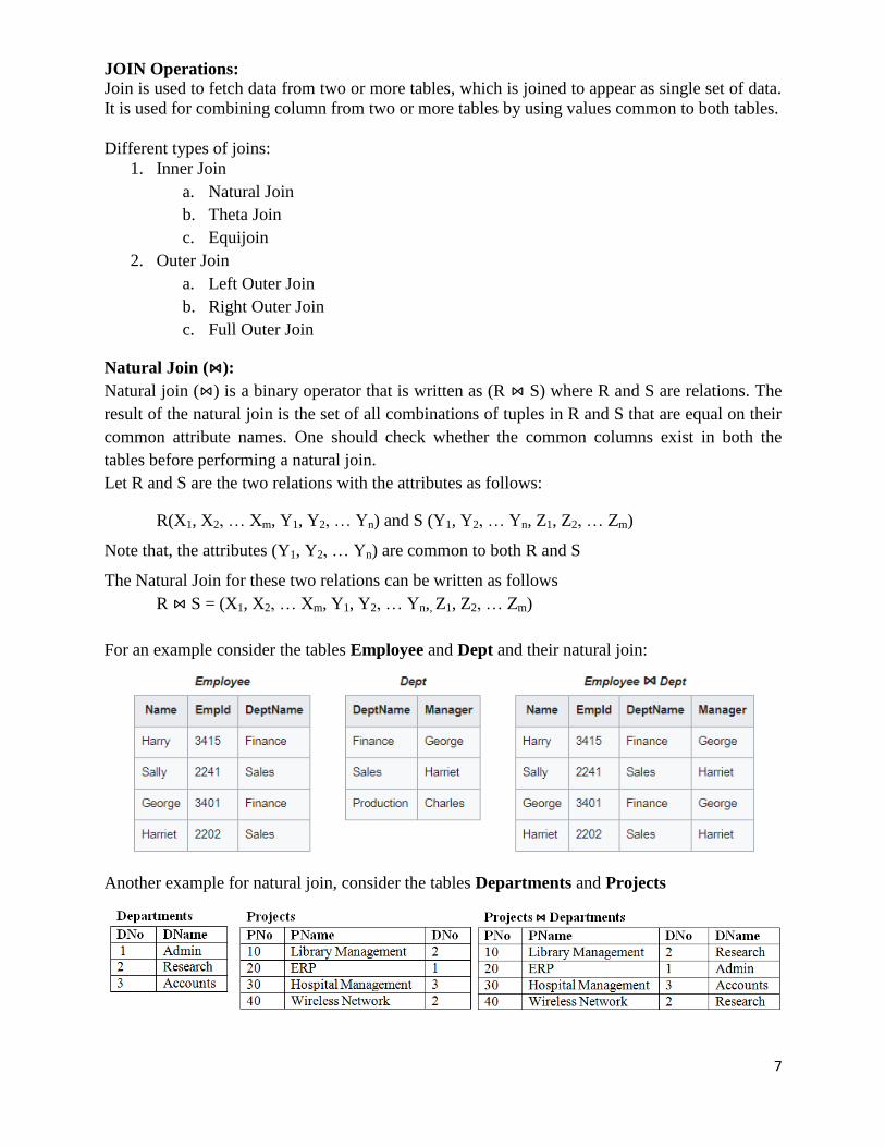
Natural Join (⋈):
Natural join (⋈) is a binary operator that is written as (R ⋈ S) where R and S are relations. The
result of the natural join is the set of all combinations of tuples in R and S that are equal on their
common attribute names. One should check whether the common columns exist in both the
tables before performing a natural join.
Let R and S are the two relations with the attributes as follows:
R(X1, X2, … Xm, Y1, Y2, … Yn) and S (Y1, Y2, … Yn, Z1, Z2, … Zm)
Note that, the attributes (Y1, Y2, … Yn) are common to both R and S
The Natural Join for these two relations can be written as follows
R ⋈ S = (X1, X2, … Xm, Y1, Y2, … Yn,, Z1, Z2, … Zm)
For an example consider the tables Employee and Dept and their natural join:
Another example for natural join, consider the tables Departments and Projects
8
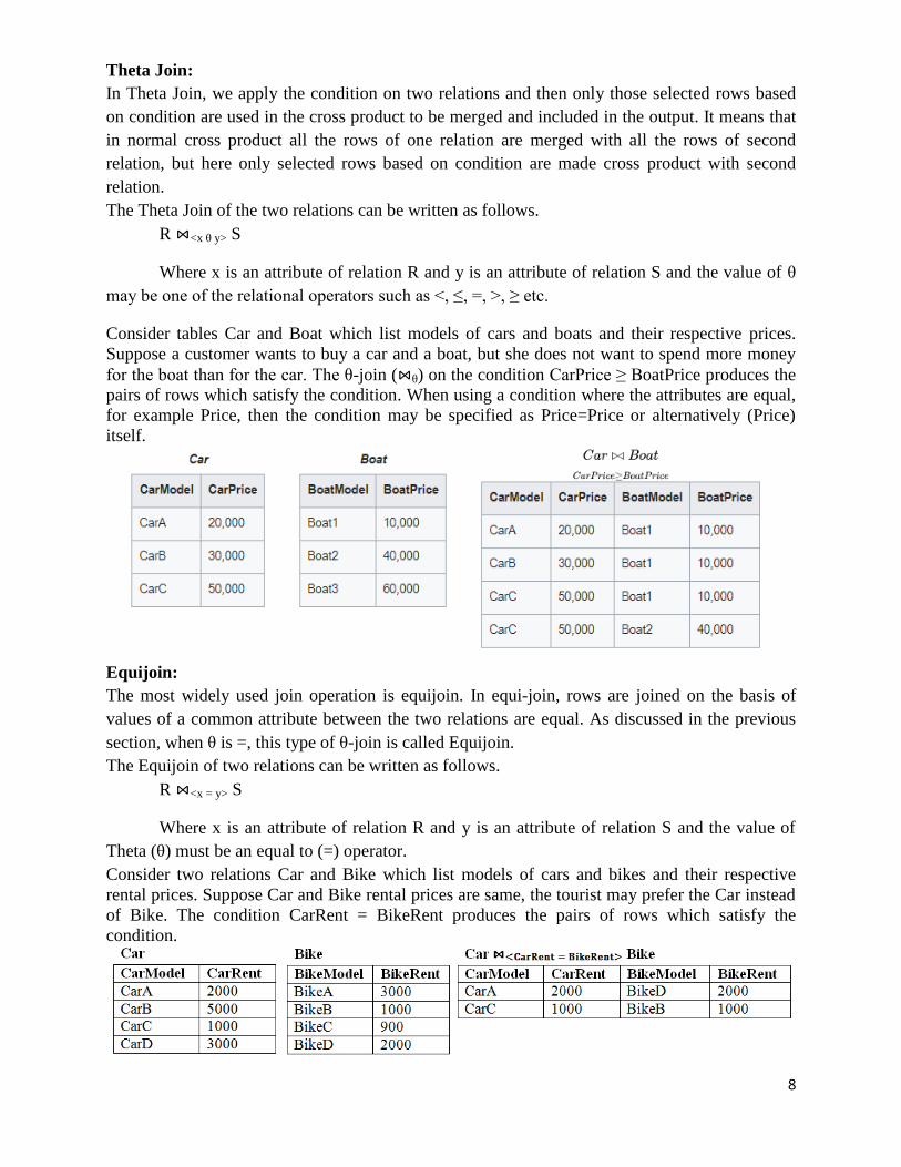
Theta Join:
In Theta Join, we apply the condition on two relations and then only those selected rows based
on condition are used in the cross product to be merged and included in the output. It means that
in normal cross product all the rows of one relation are merged with all the rows of second
relation, but here only selected rows based on condition are made cross product with second
relation.
The Theta Join of the two relations can be written as follows.
R ⋈<x θ y> S
Where x is an attribute of relation R and y is an attribute of relation S and the value of θ
may be one of the relational operators such as <, ≤, =, >, ≥ etc.
Consider tables Car and Boat which list models of cars and boats and their respective prices.
Suppose a customer wants to buy a car and a boat, but she does not want to spend more money
for the boat than for the car. The θ-join (⋈θ) on the condition CarPrice ≥ BoatPrice produces the
pairs of rows which satisfy the condition. When using a condition where the attributes are equal,
for example Price, then the condition may be specified as Price=Price or alternatively (Price)
itself.
Equijoin:
The most widely used join operation is equijoin. In equijoin, rows are joined on the basis of
values of a common attribute between the two relations are equal. As discussed in the previous
section, when θ is =, this type of θ-join is called Equijoin.
The Equijoin of two relations can be written as follows.
R ⋈<x = y> S
Where x is an attribute of relation R and y is an attribute of relation S and the value of
Theta (θ) must be an equal to (=) operator.
Consider two relations Car and Bike which list models of cars and bikes and their respective
rental prices. Suppose Car and Bike rental prices are same, the tourist may prefer the Car instead
of Bike. The condition CarRent = BikeRent produces the pairs of rows which satisfy the
condition.

9
NOTE:
A theta join allows for arbitrary comparison relationships (such as <, ≤, =, >, ≥).
An equijoin is a theta join using the equality operator (=).
A natural join is an equijoin on attributes that have the same name in each relation.
Left Outer Join (⟕):
Left Outer Join is similar to a natural join, but it returns all the rows of the table on the left side
of the join and matching rows for the table on the right side of join. The rows for which there is
no matching row on right side, the result-set will contain null. Left Outer Join is also known as
Left Join.
Let R and S be two relations and the Left Outer Join (⟕) can be written as follows.
R ⟕ S
Right Outer Join (⟖):
Right Outer Join is similar to a natural join, but it returns all the rows of the table on the right
side of the join and matching rows for the table on the left side of join. The rows for which there
is no matching row on left side, the result-set will contain null. Right Outer Join is also known as
Right Join.
Let R and S be two relations and the Right Outer Join (⟖) can be written as follows.
R ⟖ S
Full Outer Join (⟗):
Full Outer Join is similar to a natural join. It creates the result-set by combining result of both
Left Outer Join and Right Outer Join. The result-set will contain all the rows from both the
tables. The rows for which there is no matching, the result-set will contain NULL values. Full
Outer Join is also known as Full Join.
Let R and S be two relations and the Right Outer Join (⟗) can be written as follows.
R ⟗ S
10
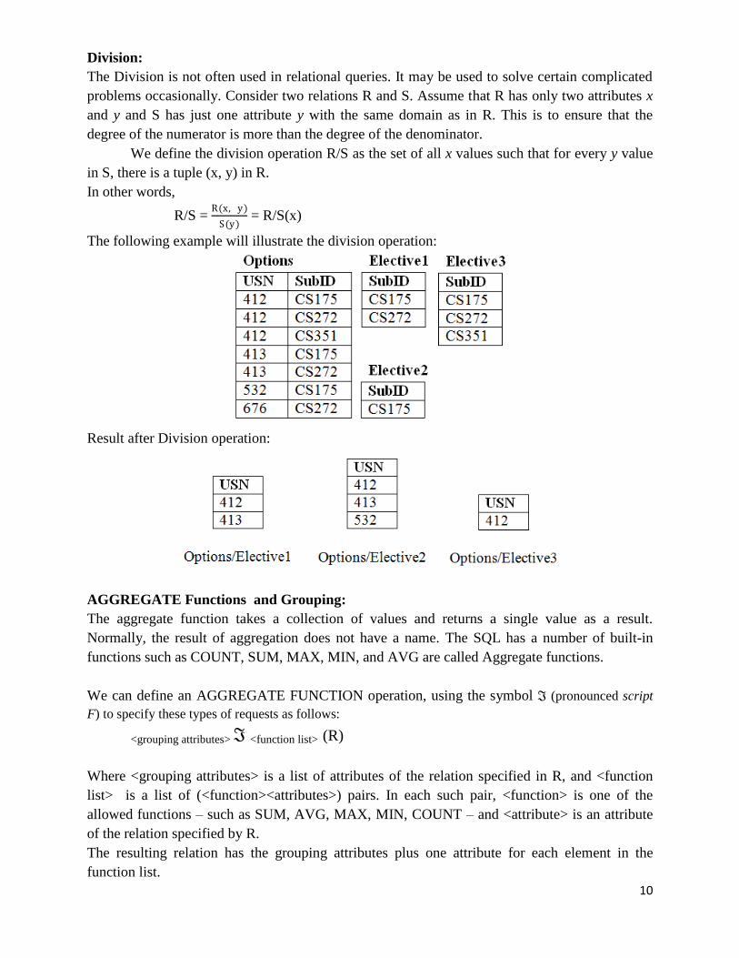
Division:
The Division is not often used in relational queries. It may be used to solve certain complicated
problems occasionally. Consider two relations R and S. Assume that R has only two attributes x
and y and S has just one attribute y with the same domain as in R. This is to ensure that the
degree of the numerator is more than the degree of the denominator.
We define the division operation R/S as the set of all x values such that for every y value
in S, there is a tuple (x, y) in R.
In other words,
R/S = R(x, y)
S(y) = R/S(x)
The following example will illustrate the division operation:
Result after Division operation:
AGGREGATE Functions and Grouping:
The aggregate function takes a collection of values and returns a single value as a result.
Normally, the result of aggregation does not have a name. The SQL has a number of built-in
functions such as COUNT, SUM, MAX, MIN, and AVG are called Aggregate functions.
We can define an AGGREGATE FUNCTION operation, using the symbol ℑ (pronounced script
F) to specify these types of requests as follows:
<grouping attributes> ℑ <function list> (R)
Where <grouping attributes> is a list of attributes of the relation specified in R, and <function
list> is a list of (<function><attributes>) pairs. In each such pair, <function> is one of the
allowed functions – such as SUM, AVG, MAX, MIN, COUNT – and <attribute> is an attribute
of the relation specified by R.
The resulting relation has the grouping attributes plus one attribute for each element in the
function list.

11
For example, to retrieve each department number, the number of employees in the department,
and their average salary, while renaming the resulting attributes as indicated below, we write:
ρR(Dno, No_of_employees, Average_sal)(Dno ℑ COUNT Ssn, AVERAGE Salary (EMPLOYEE))
The result of this operation on the EMPLOYEE relation is shown below in Figure (a). In the
above example, we specified a list of attribute names—between parentheses in the RENAME
operation—for the resulting relation R
For example, Figure (b) shows the result of the following operation:
Dno ℑ COUNT Ssn, AVERAGE Salary (EMPLOYEE)
If no grouping attributes are specified, the functions are applied to all the tuples in the relation,
so the resulting relation has a single tuple only. For example, Figure (c) shows the result of the
following operation:
ℑ COUNT Ssn, AVERAGE Salary ( EMPLOYEE)
12
Unit V
The Tuple Relational Calculus
Relational Calculus:
Relational calculus is a non-procedural query language. It uses mathematical predicate calculus
instead of algebra. Relational calculus provides the description about the query to get the result
whereas relational algebra gives the method to get the result. Relational calculus informs the
system what to do with the relation whereas relational algebra informs the system how to do with
the relation. This differs from relational algebra, which is procedural query language, where we
must write a sequence of operations to specify a retrieval request.
It has been shown that any retrieval that can be specified in the basic relational algebra can also
be specified in relational calculus, and vice versa; in other words, the expressive power of the
two languages is identical.
There are two types of relational calculus - Tuple Relational Calculus (TRC) and Domain
Relational Calculus (DRC).
Tuple Relational Calculus:
A tuple relational calculus is a non procedural query language which specifies to select a number
of tuple variables in a relation. It can select the tuples with range of values or tuples for certain
attribute values etc. The resulting relation can have one or more tuples. It is denoted as below:
{ t | condition (t) }
This is also known as expression of relational calculus
Where t is the resulting tuple (tuple variable), condition (t) is the conditional expression used to
fetch t. The result of such query is the set of all tuples t that satisfy condition (t). For example, to
find all employees whose salary is above Rs 50000, we can write the following tuple calculus
expression:
{t | EMPLOYEE (t) AND t.Salary>50000}
The above statement implies that it selects all the tuples from EMPLOYEE relation such that
resulting employee tuples will have salary greater than 50000. It is example of selecting a range
of values.
{t | EMPLOYEE (t) AND t.DEPT_ID = 10}
The above statement selects all the tuples of employee name who work for Department 10.
To retrieve only some of the attributes – say, the first name and last name and whose salary >
50000 – we write
{t.Fname, t.Lname | EMPLOYEE (t) AND t.Salary>50000}