1

Unit – VIII Graph

Prepared By:Dabbal Singh Mahara

2

Contentsa) Introduction b) b) Representation of Graph

• Array• Linked list

c) Traversals• Depth first Search• Breadth first search

d) Minimum spanning tree • Kruskal's

algorithm

3

Introduction• Graphs are a formalism for representing

relationships between objects.– a graph G is represented as G = (V, E), where,

• V is a set of vertices• E is a set of edges

Balkhu

kalanki

BafalV = {Balkhu, Kalanki, Bafal}E = {(Bafal, Kalanki), (Balkhu, Kalanki), (Kalanki, Balkhu)}

Graph• A graph G = (V,E) is composed of:

V: set of verticesE: set of edges connecting the vertices in V

• An edge e = (u,v) is a pair of vertices• Example:

a b

c

d e

V= {a,b,c,d,e}

E= {(a,b),(a,c),(a,d), (b,e),(c,d),(c,e),(d,e)}

4

5

Graph ADT

Graph Terminology:• Node

Each element of a graph is called node of a graph• Edge

Line joining two nodes is called an edge. It is denoted by e=[u,v] where u and v are adjacent vertices.

6

LoopAn edge of the form (u, u) is said to be a loop. Here in figure [v2,v2]

MultiedgeIf x was y’s friend several times over, we can model this relationship using multiedges. In figure e1 and e3.

Loop

e1

V1

V2e2V2node

edge

e3

7

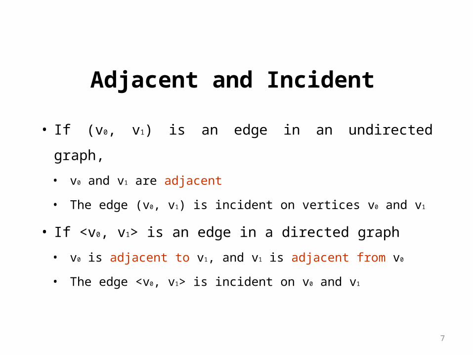
Adjacent and Incident

• If (v0, v1) is an edge in an undirected graph,

• v0 and v1 are adjacent

• The edge (v0, v1) is incident on vertices v0 and v1

• If <v0, v1> is an edge in a directed graph

• v0 is adjacent to v1, and v1 is adjacent from v0

• The edge <v0, v1> is incident on v0 and v1

8

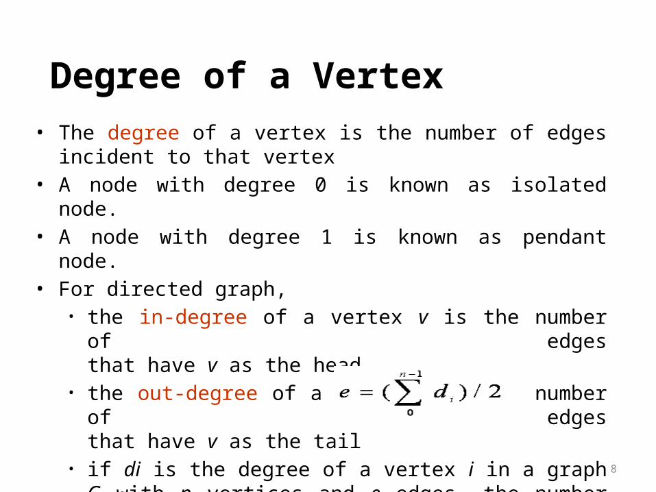
• The degree of a vertex is the number of edges incident to that vertex

• A node with degree 0 is known as isolated node.• A node with degree 1 is known as pendant node.• For directed graph,

• the in-degree of a vertex v is the number of edgesthat have v as the head

• the out-degree of a vertex v is the number of edgesthat have v as the tail

• if di is the degree of a vertex i in a graph G with n vertices and e edges, the number of edges is

Degree of a Vertex

9

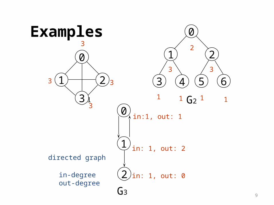
0

1 2

3 4 5 6

G1 G2

3 2

3 3

1 1 1 1

directed graph

in-degreeout-degree

0

1

2G3

in:1, out: 1

in: 1, out: 2

in: 1, out: 0

0

1 2

3

33

3

Examples

10

Path

• Path: A sequence of vertices v1,v2,. . .vk such that consecutive vertices vi and vi+1 are adjacent.

• Example: {1, 4, 3, 5, 2}

1

4 5

3

2

a b

c

d e

a b

c

d ea b e d c b e d c

• Length of a path: Number of edges on the path

• simple path: The path with no repeated vertices

• cycle: simple path, except that the last vertex is the same as the first vertex

a b

c

d e

b e c

11

• subgraph: subset of vertices and edges forming a graph• connected component: maximal connected subgraph. E.g., the graph below has

3 connected components.

connected not connected

•connected graph: any two vertices are connected by some path

12

13

Types

• Graphs are generally classified as,

• Directed graph• Undirected graph

14

Un Directed graph• A graphs G is called directed graph if each edge has no

direction.

15

• Simple GraphA graph in which there is no loop and no multiple edges between two nodes.

• Multigraph The graph which has multiple edges between any two nodes but no loops is called multigraph.

Types of Graph

16

Directed graph

• A graphs G is called directed graph if each edge has a direction.

• Pseudograph A graph which has loop is called pseudograph.

17

• Complete graph

A graph G is called complete, if every nodes are adjacent with other node

• Weighted graphIf each edge of graph is assigned a number or value, then it is weighted graph. The number is weight.

18

Why Use Graphs?

• Graphs serve as models of a wide range of objects:– A roadmap– A map of airline routes– A layout of an adventure game world– A schematic of the computers and connections that make up the

Internet– The links between pages on the Web– The relationship between students and courses– A diagram of the flow capacities in a communications or transportation

network

19

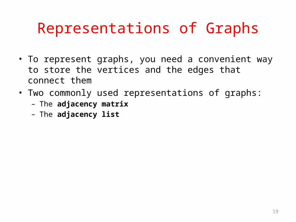
Representations of Graphs

• To represent graphs, you need a convenient way to store the vertices and the edges that connect them

• Two commonly used representations of graphs:– The adjacency matrix– The adjacency list

20

Adjacency Matrix• If a graph has N vertices labeled 0, 1, . . . , N – 1:

– The adjacency matrix for the graph is a grid G with N rows and N columns– Cell G[i][ j] = 1 if there’s an edge from vertex i to j

• Otherwise, there is no edge and that cell contains 0• These are the simplest ways for representing graphs.• Space requirement: O(n2)• Adding and deleting edge: O(1)• Testing an edge : O(1)

21

Adjacency Matrix (continued)• If the graph is undirected, then four more cells are occupied by 1:• If the vertices are labeled, then the labels can be stored in a

separate one-dimensional array

22

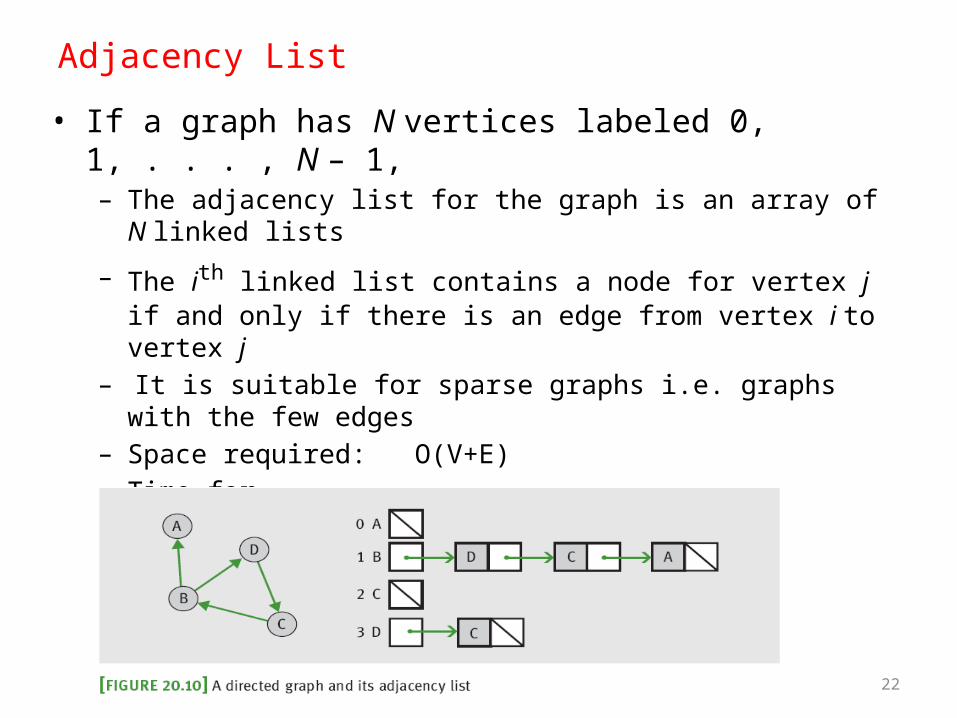
Adjacency List

• If a graph has N vertices labeled 0, 1, . . . , N – 1, – The adjacency list for the graph is an array of N linked lists

– The ith linked list contains a node for vertex j if and only if there is an edge from vertex i to vertex j

– It is suitable for sparse graphs i.e. graphs with the few edges– Space required: O(V+E)– Time for

• Testing edge to u O(dge(u))• Finding adjacent vertices: O(deg(u))• Insertion and deletion : O(deg(u))

23

Adjacency List (continued)

24

Exercise:Construct Adjacency List and Adjacency Matrix

i. ii.1

5 4

3

2

25

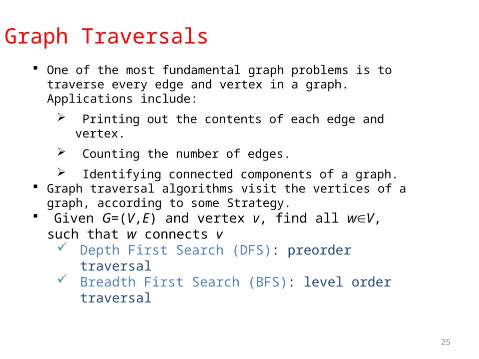
One of the most fundamental graph problems is to traverse every edge and vertex in a graph. Applications include:

Printing out the contents of each edge and vertex. Counting the number of edges. Identifying connected components of a graph.

Graph traversal algorithms visit the vertices of a graph, according to some Strategy.

Given G=(V,E) and vertex v, find all wV, such that w connects v Depth First Search (DFS): preorder traversal Breadth First Search (BFS): level order traversal

Graph Traversals

26

DFSThe basic idea is:• Start from the given vertex and go as far as possible

i.e. search continues until the end of the path if not visited already,

• Otherwise, backtrack and try another path.• DFS uses stack to process the nodes.

Algorithm:

DFS(G,S){ T = { S }; Traverse(S);}

Traverse(v){ for each w adjacent to v not yet in T {

T = T U {w}; // add edge {v,w} in TTraverse(w);

}}

27

2

1

6

7

5

3

4

Example: DFS Tracing

Starting Vertex : 1

2

1

6

7

5

3

4

Visited Nodes: T = { }2

1

6

7

5

3

4

T = { 1 }T = { 1, 2 }

28

2

1

6

7

5

3

4

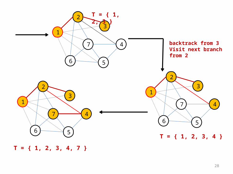
T = { 1, 2, 3 }

backtrack from 3 Visit next branch from 2

2

1

6

7

5

3

4

T = { 1, 2, 3, 4 }

2

1

6

7

5

3

4

T = { 1, 2, 3, 4, 7 }

29

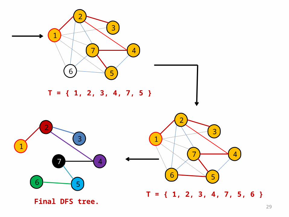
T = { 1, 2, 3, 4, 7, 5 }

2

1

6

7

5

3

4

2

1

6

7

5

3

4

T = { 1, 2, 3, 4, 7, 5, 6 }

2

1

6

7

5

3

4

Final DFS tree.

30

Analysis:• The complexity of the algorithm is greatly affected by

Traverse function we can write its running time in terms of the relation,

T(n) = T(n-1) + O(n),• At each recursive call a vertex is decreased and for

each vertex atmost n adjacent vertices can be there. So, O(n).

• Solving this we get, T(n) = O(n2). This is the case when we use adjacency matrix.

• If adjacency list is used, T(n) = O(n + e), where e is number of edges.

31

BFS• This is one of the simplest methods of graph searching. • Choose some vertex as a root or starting vertex. • Add it to the queue. Mark it as visited and dequeue it from the queue. • Add all the adjacent vertices of this node into queue.• Remove one node from front and mark it as visited. Repeat this process until all the

nodes are visited.

BFS (G, S){ Initialize Queue, q = { } mark S as visited;

enqueue(q, S);while( q != Empty){

v = dequeue(q); for each w adjacent to v

{ if w is not marked as visited {

enqueue(q, w)mark w as visited.

}}

}}

32

Analysis:

• This algorithms puts all the vertices in the queue and they are accessed one by one.

• for each accessed vertex from the queue their adjacent vertices are looked up for O(n) time (for worst case).

• Total time complexity , T(n) = O(n2) , in case of adjacency matrix.

• T(n) = O(n +e), in case of adjacency list.

33

2

1

6

7

5

3

4

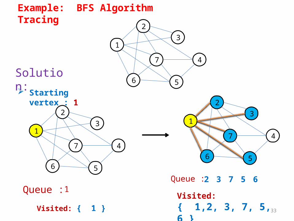
Example: BFS Algorithm Tracing

Solution:

2

1

6

7

5

3

4

Starting vertex : 1

Visited: { 1 }

2

1

6

7

5

3

4

Visited: { 1,2, 3, 7, 5, 6 }1

2 3 7 5 6Queue :Queue :

34

2

1

6

7

5

3

4

Dequeue front of queue. Add its all unvisited adjacent nodes to the queue.

Queue 3 7 5 6 4

Visited : { 1, 2, 3, 7, 5, 6, 4 }

2

1

6

7

5

3

4

Queue

Visited : { 1, 2, 3, 7, 5, 6, 4 }

35

2

1

6

7

5

3

4

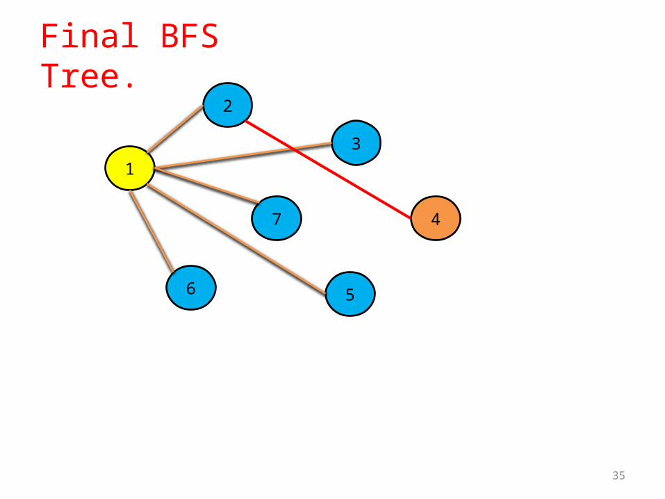
Final BFS Tree.

36

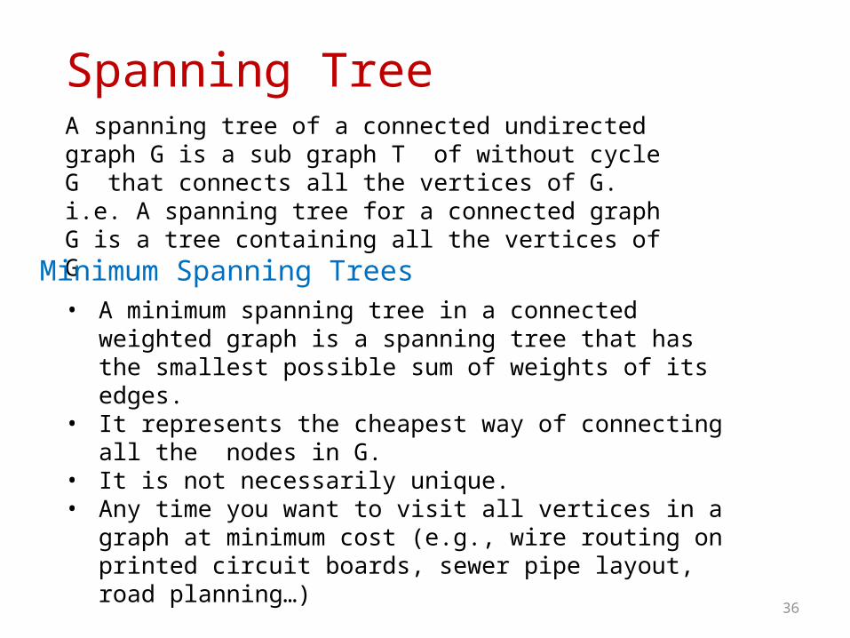
Spanning TreeA spanning tree of a connected undirected graph G is a sub graph T of without cycle G that connects all the vertices of G. i.e. A spanning tree for a connected graph G is a tree containing all the vertices of G

• A minimum spanning tree in a connected weighted graph is a spanning tree that has the smallest possible sum of weights of its edges.

• It represents the cheapest way of connecting all the nodes in G.• It is not necessarily unique.• Any time you want to visit all vertices in a graph at minimum cost

(e.g., wire routing on printed circuit boards, sewer pipe layout, road planning…)

Minimum Spanning Trees

37

• Two algorithms that are used to construct the minimum spanning tree from the given connected weighted graph of given graph are: Kruskal's Algorithm Prim's Algorithm

MST Generating Algorithms

Kruskal's AlgorithmWe have V as a set of n vertices and E as set of edges of graph G. The idea behind this algorithm is:

• The nodes of the graph are considered as n distinct partial trees with one node each.

• At each step of the algorithm, two partial trees are connected into single partial tree by an edge of the graph.

• While connecting two nodes of partial trees, minimum weighted arc is selected.

• After n-1 steps MST is obtained.

38

39

40

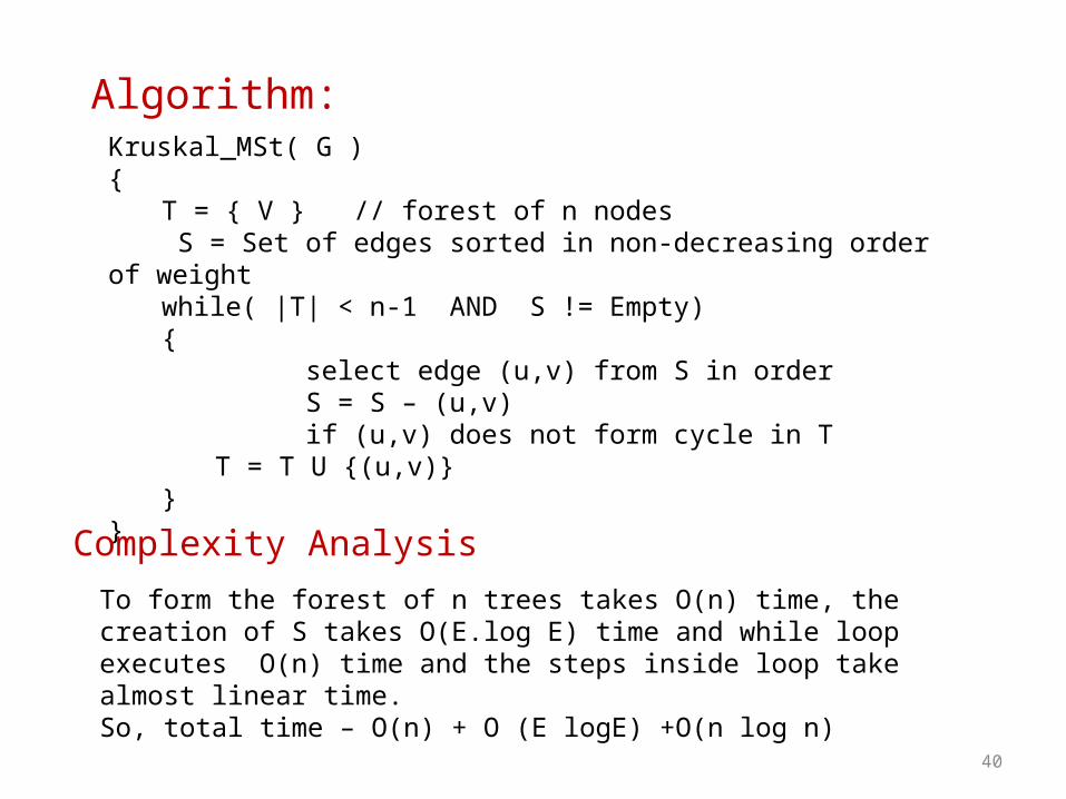
Algorithm:Kruskal_MSt( G ){

T = { V } // forest of n nodes S = Set of edges sorted in non-decreasing order of weightwhile( |T| < n-1 AND S != Empty){ select edge (u,v) from S in order S = S – (u,v) if (u,v) does not form cycle in T

T = T U {(u,v)}}

}

Complexity AnalysisTo form the forest of n trees takes O(n) time, the creation of S takes O(E.log E) time and while loop executes O(n) time and the steps inside loop take almost linear time.So, total time – O(n) + O (E logE) +O(n log n)

41

2

1

6

7

5

3

4

18

7

10

15

89

11

13

7

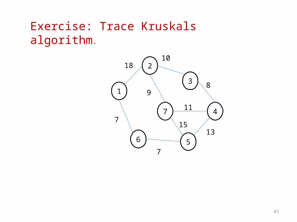
Exercise: Trace Kruskals algorithm.

42

Thank You !