UNIT 7 CELLULAR MANUFACTURING

7.1 Introduction

7.2 Coding and classification of parts

7.2.1 Mono Code or Hierarchical Code

7.2.2 Chain Code or Poly Code

7.2.3 Mixed Code or Hybrid Code

7.2.4 Group Technology Coding System

7.2.5 Code Contents

7.2.6 The Optiz System

7.2.7 The KK3 System

7.2.8 The MICLASS System

7.2.9 The DICLASS system

7.3 Machine Selection

7.4 Models For Machine cell and Part Family Formation

7.5 Production Flow Analysis

7.5.1 Rank Order Clustering

7.5.2 Bond energy algorithm

7.6 Scheduling and Control in Cellular Manufacturing

7.6.1 An Integrated GT and MRP structure

7.6.2 Operation allocation in a cell with negligible setup time

7.7 Summery

7.8 Keywords

7.9 Answer to SAQs

7.10 References

7.1 INTRODUCTION

Group technology (GT) signifies a philosophical tool, which attempts to analyze and to

arrange the parts into groups to take advantage of their similarities according to design

and production process. On the basis of groups, families can be established for

rationalizing the manufacturing process in the area of small and medium batch sizes of

mass production of a large product mix. In the cut throat competition in the global market

to meet the needs of customers, manufactures are forced to adopt the small batch

production with large production mix as compared to from mass production paradigm. To

accomplish these needs, manufactures have to adopt the method of GT to produce small

volume batches consisting of complex parts in a short production period. GT philosophy

is applied to organize a large portion of the manufacturing systems into cells, which leads

to cellular manufacturing system.

GT can be defined as “It is the realization that many problems are similar, and that by

grouping similar problems, a single solution can be found to a set of problems thus

saving time and effort”

The definition of GT is although quite broad, one usually relates GT to production flow

analysis only. GT can be applied in different area of production system. For component

design, it is obvious that many components have a similar shape. These similar

components can be grouped into design families and a new design can be created by

simply modifying an existing design from the same family. By using this concept,

composite components can be identified.

For manufacturing purposes, GT presents a greater importance than simply a design

philosophy. Similar manufacturing processes may be required for those components

which are not similar in shape. And such those components can be grouped into a cell.

The set of similar components can be called as a part family. Since all family members

require similar processes, a machine cell can be built to manufacture the family. This

makes production planning and control much easier because only similar components are

considered for each cell. Such a cell-oriented layout is called a group-technology layout

or cellular layout.

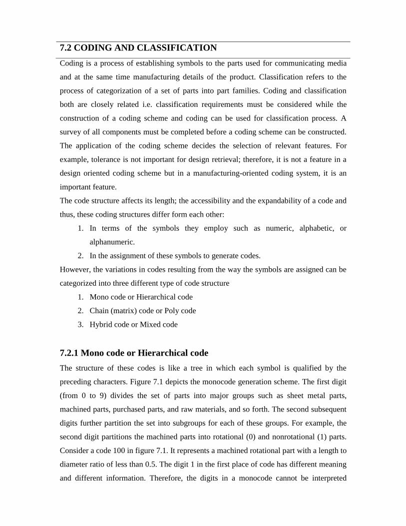
7.2 CODING AND CLASSIFICATION

Coding is a process of establishing symbols to the parts used for communicating media

and at the same time manufacturing details of the product. Classification refers to the

process of categorization of a set of parts into part families. Coding and classification

both are closely related i.e. classification requirements must be considered while the

construction of a coding scheme and coding can be used for classification process. A

survey of all components must be completed before a coding scheme can be constructed.

The application of the coding scheme decides the selection of relevant features. For

example, tolerance is not important for design retrieval; therefore, it is not a feature in a

design oriented coding scheme but in a manufacturing-oriented coding system, it is an

important feature.

The code structure affects its length; the accessibility and the expandability of a code and

thus, these coding structures differ form each other:

1. In terms of the symbols they employ such as numeric, alphabetic, or

alphanumeric.

2. In the assignment of these symbols to generate codes.

However, the variations in codes resulting from the way the symbols are assigned can be

categorized into three different type of code structure

1. Mono code or Hierarchical code

2. Chain (matrix) code or Poly code

3. Hybrid code or Mixed code

7.2.1 Mono code or Hierarchical code

The structure of these codes is like a tree in which each symbol is qualified by the

preceding characters. Figure 7.1 depicts the monocode generation scheme. The first digit

(from 0 to 9) divides the set of parts into major groups such as sheet metal parts,

machined parts, purchased parts, and raw materials, and so forth. The second subsequent

digits further partition the set into subgroups for each of these groups. For example, the

second digit partitions the machined parts into rotational (0) and nonrotational (1) parts.

Consider a code 100 in figure 7.1. It represents a machined rotational part with a length to

diameter ratio of less than 0.5. The digit 1 in the first place of code has different meaning

and different information. Therefore, the digits in a monocode cannot be interpreted

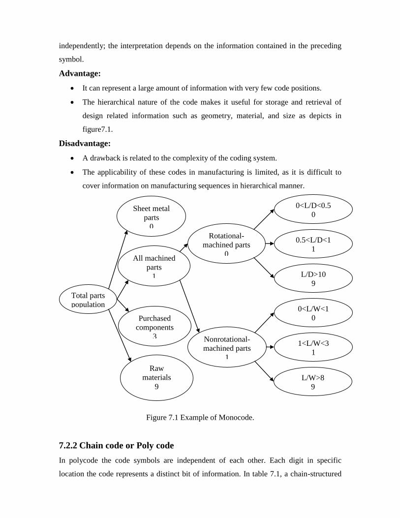
independently; the interpretation depends on the information contained in the preceding

symbol.

Advantage:

It can represent a large amount of information with very few code positions.

The hierarchical nature of the code makes it useful for storage and retrieval of

design related information such as geometry, material, and size as depicts in

figure7.1.

Disadvantage:

A drawback is related to the complexity of the coding system.

The applicability of these codes in manufacturing is limited, as it is difficult to

cover information on manufacturing sequences in hierarchical manner.

Figure 7.1 Example of Monocode.

7.2.2 Chain code or Poly code

In polycode the code symbols are independent of each other. Each digit in specific

location the code represents a distinct bit of information. In table 7.1, a chain-structured

Total parts

population

All machined

parts

1

Purchased

components

3

Raw

materials

9

Rotational-

machined parts

0

Nonrotational-

machined parts

1

0<L/D<0.5

0

0.5<L/D<1

1

L/D>10

9

0<L/W<1

0

1<L/W<3

1

Sheet metal

parts

0

L/W>8

9

coding scheme is presented. Numeral 3 in the third position always means axial and cross

hole no matter what numbers are given to position 1 and 2.

Advantages:

Chain codes are compact and are much easier to construct and use.

Disadvantage:

They cannot be as detailed as hierarchical structures with the same number of

coding digits.

Digit position 1 2 3 4

Class of features External shape Internal shape Holes …

Possible value

1 Shape 1 Shape 1 Axial …

2 Shape 1 Shape 1 cross …

3 Shape 1 Shape 1 Axial and cross …

.

.

.

.

.

.

.

.

.

.

Table 7.1 chain structure

7.2.3 Mixed code or Hybrid code

Mixed code is mixture of the hierarchical code and chain code (Figure 7.2). It retains the

advantage of both mono and chain code. Therefore, most existing code system uses a

mixed structure. One good example is widely used optiz code

Poly code Mono code Poly code

Figure 7.2 A hybrid structure

7.2.4 Group Technology Coding Systems

Too much information regarding the components sometimes makes the decision very

difficult proposition. It would be better to provide a system with an abstract kind of thing,

which can summarize the whole system with the necessary information without giving

great details.

Group technology (GT) is a fitting tool for this purpose. Coding, a GT technique, can be

used to model a component with necessary information. When constructing a coding

system for a component’s representation, there are several factors need to be considered.

They include

The population of components (i.e. rotational, prismatic, deep drawn, sheet metal,

and so on)

Detail in the code.

The code structure.

The digital representation (i.e. binary, octal, decimal, alphanumeric, hexadecimal,

and so on).

In component coding, only those features are included which are variant in nature. When

a coding scheme is designed the two criteria need to be fulfilled (1) unambiguity (2)

completeness.

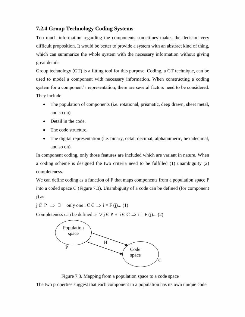
We can define coding as a function of F that maps components from a population space P

into a coded space C (Figure 7.3). Unambiguity of a code can be defined (for component

j) as

j Є P only one i Є C i = F (j)... (1)

Completeness can be defined as j Є P i Є C i = F (j)... (2)

Figure 7.3. Mapping from a population space to a code space

The two properties suggest that each component in a population has its own unique code.

Population

space

Code

space

H P

C

C

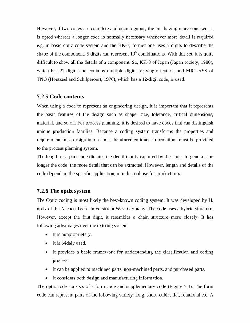
However, if two codes are complete and unambiguous, the one having more conciseness

is opted whereas a longer code is normally necessary whenever more detail is required

e.g. in basic optiz code system and the KK-3, former one uses 5 digits to describe the

shape of the component. 5 digits can represent 105 combinations. With this set, it is quite

difficult to show all the details of a component. So, KK-3 of Japan (Japan society, 1980),

which has 21 digits and contains multiple digits for single feature, and MICLASS of

TNO (Houtzeel and Schilperoort, 1976), which has a 12-digit code, is used.

7.2.5 Code contents

When using a code to represent an engineering design, it is important that it represents

the basic features of the design such as shape, size, tolerance, critical dimensions,

material, and so on. For process planning, it is desired to have codes that can distinguish

unique production families. Because a coding system transforms the properties and

requirements of a design into a code, the aforementioned informations must be provided

to the process planning system.

The length of a part code dictates the detail that is captured by the code. In general, the

longer the code, the more detail that can be extracted. However, length and details of the

code depend on the specific application, in industrial use for product mix.

7.2.6 The optiz system

The Optiz coding is most likely the best-known coding system. It was developed by H.

optiz of the Aachen Tech University in West Germany. The code uses a hybrid structure.

However, except the first digit, it resembles a chain structure more closely. It has

following advantages over the existing system

It is nonproprietary.

It is widely used.

It provides a basic framework for understanding the classification and coding

process.

It can be applied to machined parts, non-machined parts, and purchased parts.

It considers both design and manufacturing information.

The optiz code consists of a form code and supplementary code (Figure 7.4). The form

code can represent parts of the following variety: long, short, cubic, flat, rotational etc. A

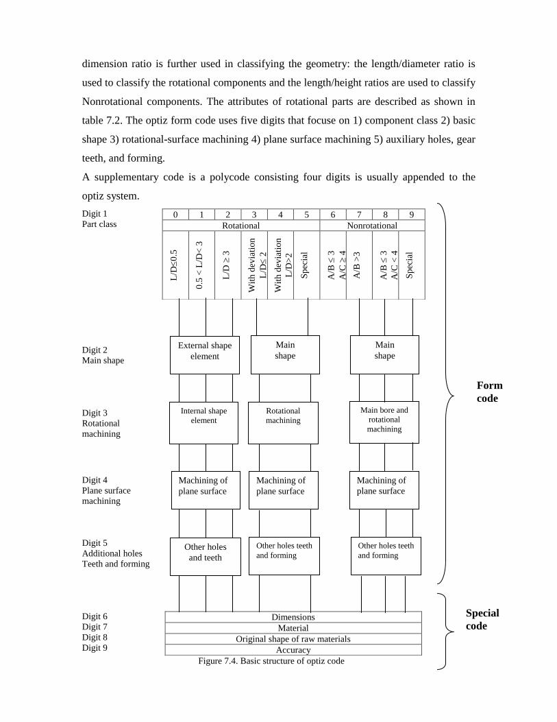
dimension ratio is further used in classifying the geometry: the length/diameter ratio is

used to classify the rotational components and the length/height ratios are used to classify

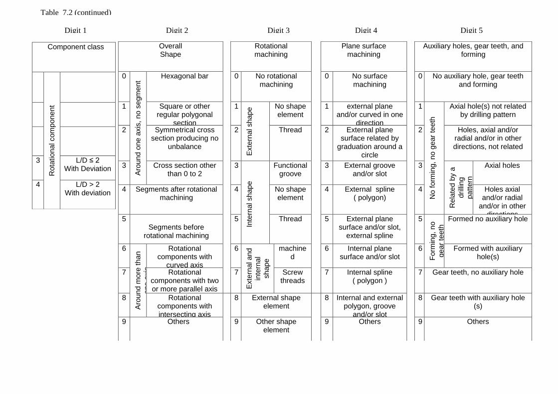
Nonrotational components. The attributes of rotational parts are described as shown in

table 7.2. The optiz form code uses five digits that focuse on 1) component class 2) basic

shape 3) rotational-surface machining 4) plane surface machining 5) auxiliary holes, gear

teeth, and forming.

A supplementary code is a polycode consisting four digits is usually appended to the

optiz system.

Digit 1

Part class

Digit 2

Main shape

Digit 3

Rotational

machining

Digit 4

Plane surface

machining

Digit 5

Additional holes

Teeth and forming

Digit 6

Digit 7

Digit 8

Digit 9

Figure 7.4. Basic structure of optiz code

0 1 2 3 4 5 6 7 8 9

Rotational Nonrotational

L/D

0.5

0.5

< L

/D<

3

L/D

3

Wit

h d

evia

tio

n

L/D

2

Wit

h d

evia

tio

n

L/D

>2

Sp

ecia

l

A/B

3

A/C

4

A/B

>3

A/B

3

A/C

< 4

Sp

ecia

l

Dimensions

Material

Original shape of raw materials

Accuracy

Form

code

External shape

element

Main

shape

Main

shape

Internal shape

element

Rotational

machining

Main bore and

rotational

machining

Machining of

plane surface

Machining of

plane surface

Machining of

plane surface

Other holes

and teeth

Other holes teeth

and forming

Other holes teeth

and forming

Special

code

Form code (digit 1-5) for rational parts in the optiz system. Part classes 0, 1, and 2.

Digit 1 Digit 2 Digit 3 Digit 4 Digit 5

Table 7.2 (continued)

Part class External shape, external shape

element

Internal shape, internal shape

element

Plane surface machining

Auxiliary holes and gear teeth

0 N

onro

tatio

na

l p

art

s R

ota

tio

na

l p

art

s

L/D ≤ 0.5 0 Smooth no shape element

0 No hole, no breakthrough

0 No surface machining

0

With

gear

teeth

n

o g

ea

r te

eth

No auxiliary hole

1 0.5 < L/D < 3 1

Ste

pp

ed

at

one e

nd No shape

element 1

Sm

ooth

or

ste

pp

ed

to o

ne e

nd

No shape element

1 Surface plane and/or curved in

one direction

1 Axial, not on pitch circle diameter

2 L/D ≥ 3 2 Smooth thread

2 Thread 2 External plane surface related by

graduation around a circle

2 Axial on pitch circle diameter

3 3 Smooth functional

groove

3 Functional groove

3 External groove and/or slot

3 Radial, not on pitch circle diameter

4 4

Ste

pp

ed

at

both

en

d No shape

element 4

Ste

pp

ed

at

both

en

d No shape

element 4 External spline

( polygon) 4 Axial and/or radial

and/or other direction

5 5 Thread 5 Thread 5 External plane surface and/or slot,

external spline

5 Axial and/or radial on

pitch circle diameter

and/or other direction

6 6 Functional groove

6 Functional groove

6 Internal plane surface and/or slot

6 spur gear teeth

7 7 Functional cone 7 Functional cone 7 Internal spline ( polygon )

7 Bevel gear teeth

8 8 Operating thread 8 Operating thread 8 Internal and external polygon, groove and/or slot

8 Other gear teeth

9 9 All others 9 All others 9 All others 9 All others

Component class

Ro

tatio

na

l com

pon

en

t

3 L/D ≤ 2 With Deviation

4 L/D > 2 With deviation

Overall Shape

Rotational machining

Plane surface machining

Auxiliary holes, gear teeth, and forming

0

Aro

un

d o

ne

axis

, n

o s

egm

ent

Hexagonal bar 0 No rotational machining

0 No surface machining

0 No auxiliary hole, gear teeth and forming

1 Square or other regular polygonal

section

1

Exte

rna

l sh

ap

e No shape

element 1 external plane

and/or curved in one direction

1

No

fo

rmin

g, n

o g

ear

teeth

Axial hole(s) not related by drilling pattern

2 Symmetrical cross section producing no

unbalance

2 Thread 2 External plane surface related by

graduation around a circle

2 Holes, axial and/or radial and/or in other directions, not related

3 Cross section other than 0 to 2

3

Inte

rnal sh

ap

e

Functional groove

3 External groove and/or slot

3

Re

late

d b

y a

drilli

ng

patt

ern

Axial holes

4 Segments after rotational machining

4 No shape element

4 External spline ( polygon)

4

Holes axial and/or radial

and/or in other directions

5 Segments before

rotational machining

5 Thread 5 External plane surface and/or slot,

external spline

5

Form

ing, n

o

gea

r te

eth

Formed no auxiliary hole

6

Aro

un

d m

ore

th

an

one

axis

Rotational components with

curved axis

6 E

xte

rna

l a

nd

inte

rnal

sh

ap

e

machined

6 Internal plane surface and/or slot

6 Formed with auxiliary hole(s)

7 Rotational components with two or more parallel axis

7 Screw threads

7 Internal spline ( polygon )

7 Gear teeth, no auxiliary hole

8 Rotational components with intersecting axis

8 External shape element

8 Internal and external polygon, groove

and/or slot

8 Gear teeth with auxiliary hole (s)

9 Others 9 Other shape element

9 Others 9 Others

Digit 1 Digit 2 Digit 3 Digit 4 Digit 5

Table 7.2 (continued)

Digit 1 Digit 2 Digit 3 Digit 4

Diameter D or edge length A Material Initial form Accuracy in coded digits

0 mm Inches 0 Cast iron 0 Round bar, black 0 No accuracy specified

≤ 20 ≤ 0.8

1 > 20 ≤ 50 > 0.8 ≤ 2.0 1 Modular graphitic cast iron and

malleable cast iron 1 Round bar, bright drawn 1 2

2 > 50 ≤ 100 > 2.0 ≤ 4.0 2 Mild steel ≤ 26.5 tonf/in.2

Not heat treated 2 Bar: triangular, square,

hexagonal, others 2 3

3 > 100 ≤ 160 > 4.0 ≤ 6.5 3 Hard steel > 26.5 tonf/ in.2 heat

treatable low-carbon and case-hardening steel, not heat treated

3 Tubing 3 4

4 > 160 ≤ 250 > 6.5 ≤

10.0 4 Steel 2 and 3

heat treated 4 Angle, U-, T- , and similar

sections. 4 5

5 > 250 ≤ 400 >10.0≤

16.0 5 Alloy steel

(not heat treaded) 5 Sheet 5 2 and 3

6 > 400 ≤ 600 >16.0≤

25.0 6 Alloy steel

heat treated 6 Plate and slab 6 2 and 4

7 > 600 ≤ 1000

>25.0≤ 40.0

7 Nonferrous metal 7 Cast and forge Component

7 2 and 5

8 >1000≤ 2000

>40.0≤ 80.0

8 Light alloy 8 Welded assembly 8 3 and 4

9 > 2000 >80.0 9 Other materials 9 Premachined components 9 2+3+4+5

Table 7.2 concluded

Example 7.1:

A part design is shown in figure. Develop an optiz code for that design

By using information from figure 7.5, the form code with explanation is given below

Part class:

Form code

Form code 1 3 1 0 6

Rotational part, L/D = 9.9/4.8 = 2.0 (nearly) based on the pitch circle diameter of

the gear. Therefore, the first digit would be 1.

External shape:

The part is stepped in one side with a functional groove. Therefore, the second digit

will be 3.

Internal shape:

Due to the hole the third digit code is one.

Plain surface machining:

Since, there is no surface machining the fourth digit is 0.

Auxiliary holes and gear teeth:

Because there are spur gear teeth on the part the fifth digit is 6.

7.2.7 The KK3 system The KK3 system is one of the general-purpose classification and coding system for

machined parts. It was developed by the Japanese society for the encouragement of the

machined industry.

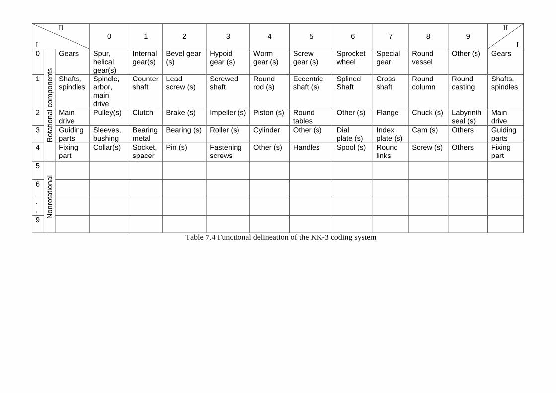
KK-3 was first presented in 1976 and use a 21-digit decimal system. Table 7.3 and 7.4

show the code structure for rational component. It can represent more information than that

of optiz code because of greater length.

5.6 2

0.3

2

Spur gear

4.8 pitch circle diameter

(p.c.d; φ) -4φ -4.3φ

Figure 7.5

It includes two digits for component name or functional name classification. First digits

classify the general function, such as gears, shafts, drive and moving parts, and fixing parts.

The second digit describes more detailed function such as spur gears, bevel gears, worm

gears, and so on.

KK-3 also classifies materials using two-code digit. The first digit classifies material type

and second digit classifies shape of the raw material. Length, diameter, and length/diameter

ratios are classified for rotational components. Shape details and types of processes are

classified using 13 digits of code. At last one digit is required for accuracy presentation. An

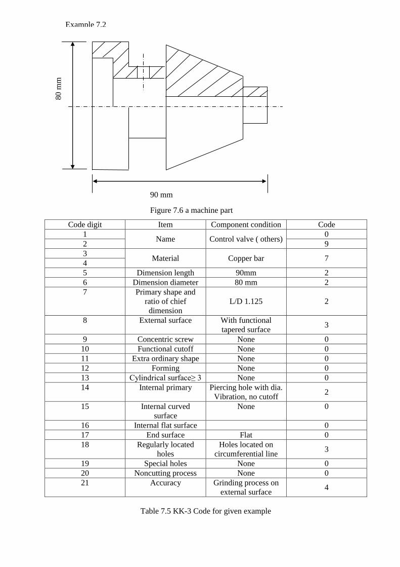
example of coding a component using KK-3 is illustrated in figure 7.6 and table 7.5.

Digit Items (rotational component)

1 Parts name

General classification

2 Detail classification

3 Materials

General classification

4 Detail classification

5 Chief dimension

Length

6 Diameter

7 Primary shapes and length diameter ratio

8

Sh

ap

e d

eta

ils a

nd k

inds o

f pro

cesse

s

External surface

External surface and outer primary shape

9 Concentric screw threaded parts

10 Functional cut-off parts

11 Extraordinary shaped parts

12 Forming

13 Cylindrical surface

14

Internal surface

Internal primary shape

15 Internal curved surface

16 Internal flat surface and cylindrical surface

17 End surface

18 Nonconcentric holes

Regularly located holes

19 Special holes

20 Noncutting process

21 Accuracy

Table 7.3 Structure of the KK-3 coding system (rotational components)

II

I 0 1 2 3 4 5 6 7 8 9

II

I

0 R

ota

tio

na

l com

pon

en

ts

Gears Spur, helical gear(s)

Internal gear(s)

Bevel gear (s)

Hypoid gear (s)

Worm gear (s)

Screw gear (s)

Sprocket wheel

Special gear

Round vessel

Other (s) Gears

1 Shafts, spindles

Spindle, arbor, main drive

Counter shaft

Lead screw (s)

Screwed shaft

Round rod (s)

Eccentric shaft (s)

Splined Shaft

Cross shaft

Round column

Round casting

Shafts, spindles

2 Main drive

Pulley(s) Clutch Brake (s) Impeller (s) Piston (s) Round tables

Other (s) Flange Chuck (s) Labyrinth seal (s)

Main drive

3 Guiding parts

Sleeves, bushing

Bearing metal

Bearing (s) Roller (s) Cylinder Other (s) Dial plate (s)

Index plate (s)

Cam (s) Others Guiding parts

4 Fixing part

Collar(s) Socket, spacer

Pin (s) Fastening screws

Other (s) Handles Spool (s) Round links

Screw (s) Others Fixing part

5

No

nro

tatio

na

l

6

.

.

9

Table 7.4 Functional delineation of the KK-3 coding system

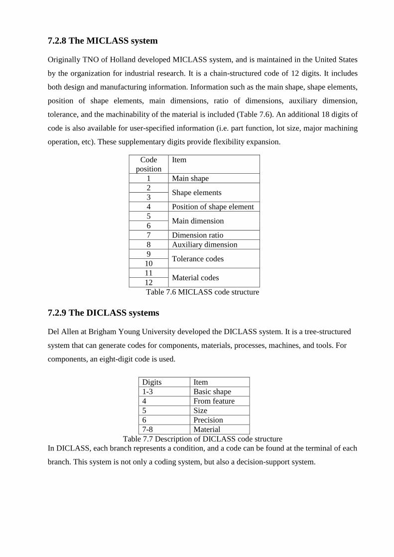
Code digit Item Component condition Code

1 Name Control valve ( others)

0

2 9

3 Material Copper bar 7

4

5 Dimension length 90mm 2

6 Dimension diameter 80 mm 2

7 Primary shape and

ratio of chief

dimension

L/D 1.125 2

8 External surface With functional

tapered surface 3

9 Concentric screw None 0

10 Functional cutoff None 0

11 Extra ordinary shape None 0

12 Forming None 0

13 Cylindrical surface≥ 3 None 0

14 Internal primary Piercing hole with dia.

Vibration, no cutoff 2

15 Internal curved

surface

None 0

16 Internal flat surface 0

17 End surface Flat 0

18 Regularly located

holes

Holes located on

circumferential line 3

19 Special holes None 0

20 Noncutting process None 0

21 Accuracy Grinding process on

external surface 4

Table 7.5 KK-3 Code for given example

90 mm

80 m

m

Figure 7.6 a machine part

Example 7.2

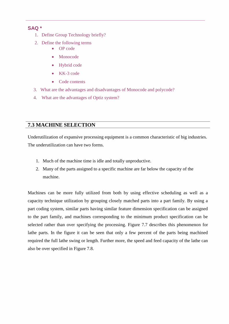
7.2.8 The MICLASS system

Originally TNO of Holland developed MICLASS system, and is maintained in the United States

by the organization for industrial research. It is a chain-structured code of 12 digits. It includes

both design and manufacturing information. Information such as the main shape, shape elements,

position of shape elements, main dimensions, ratio of dimensions, auxiliary dimension,

tolerance, and the machinability of the material is included (Table 7.6). An additional 18 digits of

code is also available for user-specified information (i.e. part function, lot size, major machining

operation, etc). These supplementary digits provide flexibility expansion.

Code

position

Item

1 Main shape

2 Shape elements

3

4 Position of shape element

5 Main dimension

6

7 Dimension ratio

8 Auxiliary dimension

9 Tolerance codes

10

11 Material codes

12

Table 7.6 MICLASS code structure

7.2.9 The DICLASS systems

Del Allen at Brigham Young University developed the DICLASS system. It is a tree-structured

system that can generate codes for components, materials, processes, machines, and tools. For

components, an eight-digit code is used.

Digits Item

1-3 Basic shape

4 From feature

5 Size

6 Precision

7-8 Material

Table 7.7 Description of DICLASS code structure

In DICLASS, each branch represents a condition, and a code can be found at the terminal of each

branch. This system is not only a coding system, but also a decision-support system.

SAQ *

1. Define Group Technology briefly?

2. Define the following terms

OP code

Monocode

Hybrid code

KK-3 code

Code contents

3. What are the advantages and disadvantages of Monocode and polycode?

4. What are the advantages of Optiz system?

7.3 MACHINE SELECTION

Underutilization of expansive processing equipment is a common characteristic of big industries.

The underutilization can have two forms.

1. Much of the machine time is idle and totally unproductive.

2. Many of the parts assigned to a specific machine are far below the capacity of the

machine.

Machines can be more fully utilized from both by using effective scheduling as well as a

capacity technique utilization by grouping closely matched parts into a part family. By using a

part coding system, similar parts having similar feature dimension specification can be assigned

to the part family, and machines corresponding to the minimum product specification can be

selected rather than over specifying the processing. Figure 7.7 describes this phenomenon for

lathe parts. In the figure it can be seen that only a few percent of the parts being machined

required the full lathe swing or length. Further more, the speed and feed capacity of the lathe can

also be over specified in Figure 7.8.

Actual vs Available Machine Capacity

0

5

10

15

20

25

30

35

<1 1.0-3.0 3.0-6.0 6.0-

12.0

12.0-

20.0

20.0-

40.0

40.0-

80.0

>80

Diameter(inches)

Pe

rce

nt

Actual part diameter

Available machine capicity

Figure 7.7 Comparision of a turned-part dimension as a function

of machine capacity

0

5

10

15

20

25

30

35

40

45

<1.00 1.00-

3.00

3.00-

6.00

6.00-

12.00

12.00-

20.00

20.00-

40.00

40.00-

80.00

>80.00

Length

Perc

ent Actual Part lengths

Available Machine

Capacity

Actual vs Available Machine Capacity

0

5

10

15

20

25

30

35

40

45

Maximum Speed(RPM)

Pe

rce

nt

Actual Part

Speeds

Available

Machine

Capacity

Figure 7.8 Comparision of maximum speeds and feeds

with maximum used

0

5

10

15

20

25

30

35

Maximum feed (Inch/Rev)

Pe

rce

nt

Actual Part

Speeds

Available

Machine

Capacity

7.4 MODELS FOR MACHINE CELL AND PART FAMILY FORMATION

One of the primary uses of coding system in manufacturing is to develop part families for

efficient workflow. Efficient workflow can result from grouping machines logically so that

material handling and setup can be minimized. The same tools and fixtures can be used by

grouping parts having similar operations. Due to this, a major reduction in setup results and also

material handling between machining operations is minimized.

Family formation is based on production parts or more specifically, their manufacturing feature.

Components requiring similar processing are grouped into the same family. There is no rigid rule

that can be applied to form families because a part family is loosely defined. A general rule for

part family formation is that all parts in a family must be related that is all parts in a family must

require similar routing. A user may want to put only those parts having exactly the same routing

sequence into a family. Minimum modification on the standard route is required for such family

members. Only, few parts will qualify for family membership. On the other hand, if one groups

all the parts requiring a common machine into family, large part families will results.

Before grouping can start, information related to the design and processing of all existing

components have to be collected from existing part and processing files. Each component is

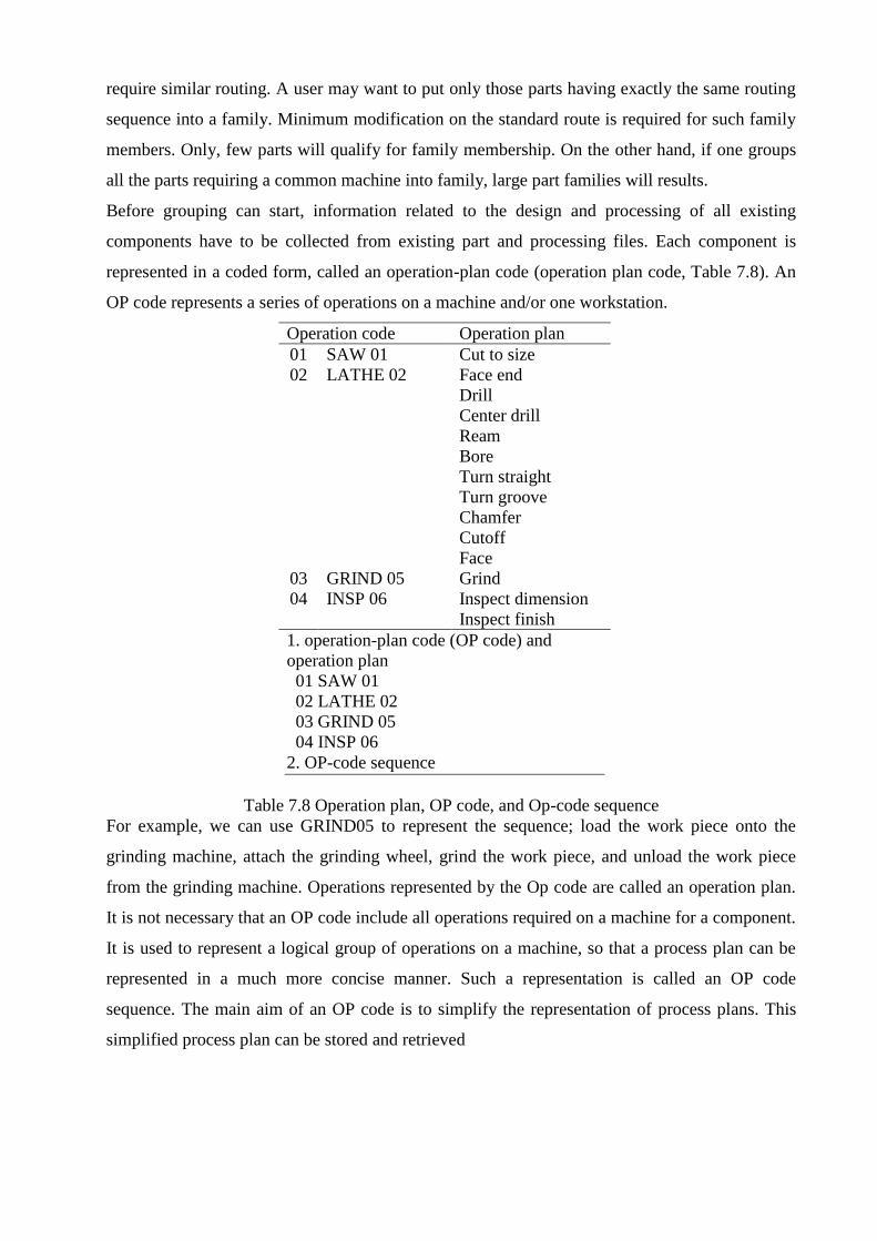
represented in a coded form, called an operation-plan code (operation plan code, Table 7.8). An

OP code represents a series of operations on a machine and/or one workstation.

Operation code Operation plan

01 SAW 01 Cut to size

02 LATHE 02 Face end

Drill

Center drill

Ream

Bore

Turn straight

Turn groove

Chamfer

Cutoff

Face

03 GRIND 05 Grind

04 INSP 06 Inspect dimension

Inspect finish

1. operation-plan code (OP code) and

operation plan

01 SAW 01

02 LATHE 02

03 GRIND 05

04 INSP 06

2. OP-code sequence

Table 7.8 Operation plan, OP code, and Op-code sequence

For example, we can use GRIND05 to represent the sequence; load the work piece onto the

grinding machine, attach the grinding wheel, grind the work piece, and unload the work piece

from the grinding machine. Operations represented by the Op code are called an operation plan.

It is not necessary that an OP code include all operations required on a machine for a component.

It is used to represent a logical group of operations on a machine, so that a process plan can be

represented in a much more concise manner. Such a representation is called an OP code

sequence. The main aim of an OP code is to simplify the representation of process plans. This

simplified process plan can be stored and retrieved

7.5 PRODUCTION FLOW ANALYSIS

Production flow analysis (PFA) was established by J. Burbidge to solve the family-formation

problem for manufacturing cell design. This analysis uses the information contained on

production route sheets. Work parts with identical or similar routing are classified into part

families which can be used to form logical machine cells in a group technology layout. Since

PFA uses manufacturing data rather than design data to identify part families, it can overcome

two possible abnormalities that can occur in part classification and coding. First, parts whose

basic geometries are quite different may nevertheless require similar or identical process routing.

Second, parts whose geometries are quite similar may nevertheless require process routing that

are quite different.

The procedure in PFA consists of the following steps.

Machine classification. Classification of machines is based on the operation that can be

performed on them. A machine type is assigned to machines capable of performing

similar operations.

Checking part list and production route information. For each parts, information on the

operations to be taken and the machines required to perform each of these operations is

checked carefully

Factory flow analysis. This comprise a micro level examination of flow of components

through machines. Thus, it allows the problem to be decomposed into a number of

machine-component groups.

Machine-component group analysis. This analysis recommended manipulating the

matrix to form cells.

Many researchers have been subsequently developed algorithm to solve the family-formation

problem for manufacturing cell design. In PFA, a large matrix generally termed as incidence is

constructed. Each row represents an OP code, and each column represents a component. We can

define the matrix as Mij, where i indicates the optiz code and j indicates components for example

Mij = 1 if component j has OP code i; otherwise Mij = 0. The objective of PFA is to bring

together those components that need the similar set of OP codes in clusters.

7.5.1 Rank order clustering

This method is based on sorting the rows and columns of machine part incidence matrix. The

rank order clustering was developed by King (1980). Steps of this algorithm is given below

Step 1. For each row of the machine part incidence matrix, assign binary weight and calculate the

decimal equivalent

Step 2. Sort rows of the binary matrix in decreasing order of the corresponding decimal weights.

11

20

10

20

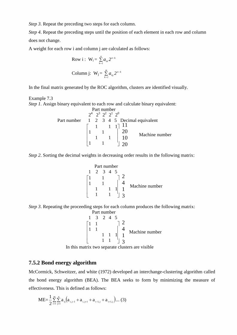
Step 3. Repeat the preceding two steps for each column.

Step 4. Repeat the preceding steps until the position of each element in each row and column

does not change.

A weight for each row i and column j are calculated as follows:

Row i : Wi =

n

1k

kn

ik2a

Column j: Wj =

m

1k

kn

kj2a

In the final matrix generated by the ROC algorithm, clusters are identified visually.

Example 7.3

Step 1. Assign binary equivalent to each row and calculate binary equivalent:

Part number

24 2

3 2

2 2

1 2

0

Part number 1 2 3 4 5 Decimal equivalent

11

11

11

111

Machine number

Step 2. Sorting the decimal weights in decreasing order results in the following matrix:

Part number

1 2 3 4 5

11

111

11

11

Machine number

Step 3. Repeating the proceeding steps for each column produces the following matrix:

Part number

1 3 2 4 5

11

111

11

11

Machine number

In this matrix two separate clusters are visible

7.5.2 Bond energy algorithm

McCormick, Schweitzer, and white (1972) developed an interchange-clustering algorithm called

the bond energy algorithm (BEA). The BEA seeks to form by minimizing the measure of

effectiveness. This is defined as follows:

ME=

m

1i

n

1jj,1ij,1i1j,i1j,iij

aaaaa2

1... (3)

2

4

1

3

2

4

1

3

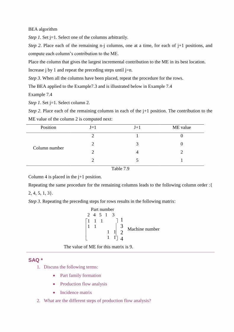
BEA algorithm

Step 1. Set j=1. Select one of the columns arbitrarily.

Step 2. Place each of the remaining n-j columns, one at a time, for each of j+1 positions, and

compute each column’s contribution to the ME.

Place the column that gives the largest incremental contribution to the ME in its best location.

Increase j by 1 and repeat the preceding steps until j=n.

Step 3. When all the columns have been placed, repeat the procedure for the rows.

The BEA applied to the Example7.3 and is illustrated below in Example 7.4

Example 7.4

Step 1. Set j=1. Select column 2.

Step 2. Place each of the remaining columns in each of the j+1 position. The contribution to the

ME value of the column 2 is computed next:

Position J=1 J+1 ME value

Column number

2 1 0

2 3 0

2 4 2

2 5 1

Table 7.9

Column 4 is placed in the j+1 position.

Repeating the same procedure for the remaining columns leads to the following column order :{

2, 4, 5, 1, 3}.

Step 3. Repeating the preceding steps for rows results in the following matrix:

Part number

2 4 5 1 3

11

11

11

111

Machine number

The value of ME for this matrix is 9.

SAQ *

1. Discuss the following terms:

Part family formation

Production flow analysis

Incidence matrix

2. What are the different steps of production flow analysis?

1

3

2

4

3. What is rank order clustering?

7.6 SCHEDULING AND CONTROL IN CELLULAR MANUFACTURING

This section discusses some issues related to scheduling and control in cellular manufacturing. In

cellular manufacturing systems, scheduling problems different form those in traditional

production systems due to certain uniqueness like

1. Machines are more flexible in performing various operations.

2. Use of group tooling significantly reduces setup time.

3. Low demands and large variety of products

4. Fewer machines than part types.

These characteristics alter the nature of scheduling problems in GT-cellular manufacturing

systems and allow us to take benefit of similarities of setups and operations by integrating GT

concept with material requirement planning (MRP). A hierarchical approach to cell planning and

control, integrating the concepts of GT and MRP, is given here. We discuss using suitable

examples how the concepts of GT and MRP can be used together to provide an efficient tool for

scheduling and control of a cellular manufacturing system.

We know that GT is one of the useful approaches to small-lot, multiproduct production system,

and MRP is an effective scheduling and control system for a batch type of production system.

Optimal lot sizes are determined for various parts required for products in an MRP system.

However, similarities among the parts requiring similar setups and operations will reduce setup

time. On the other hand, the time-phased requirement scheduling aspect is not considered in GT.

It means, all the parts in a group are assumed to be available at the beginning of the period.

Evidently, a better scheduling and control system will be achieved by integration of GT and

MRP. For scheduling and control in cellular manufacturing systems an integrated GT and MRP

framework are defined in the next subsection.

7.6.1 An Integrated GT and MRP structure

The goal of an integrated GT and MRP framework is to take advantage of the similarities of

setups and operations from GT and time-phased requirements from MRP. This can be achieved

through a series of simple steps as follows:

Step I. Collects the data that are normally required for both the GT and MRP concepts (that is,

machine capabilities, parts and their description, a break down of each final product into its

individual components, a forecast of final product demand, and so forth).

Step II. Use GT procedures for determining the part families. Designate each families as GI (I=1,

2, 3,…, N)

Step III. Use MRP for assigning each part to a specific time period.

Step IV. Arrange the component part-time period assignments of step III according to part family

groups of step II.

Step V. Use a suitable group scheduling algorithm to determine the optimal schedule for all the

parts within a given group for each time period.

We now illustrate the integrated framework with a simple example.

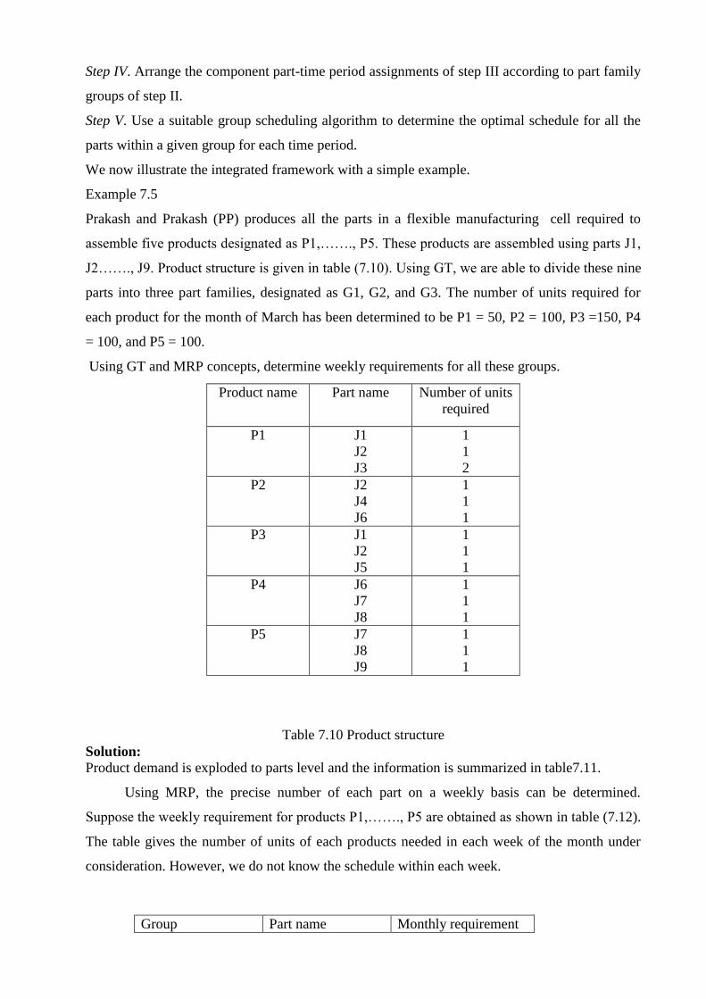
Example 7.5

Prakash and Prakash (PP) produces all the parts in a flexible manufacturing cell required to

assemble five products designated as P1,……., P5. These products are assembled using parts J1,

J2……., J9. Product structure is given in table (7.10). Using GT, we are able to divide these nine

parts into three part families, designated as G1, G2, and G3. The number of units required for

each product for the month of March has been determined to be P1 = 50, P2 = 100, P3 =150, P4

= 100, and P5 = 100.

Using GT and MRP concepts, determine weekly requirements for all these groups.

Table 7.10 Product structure

Solution:

Product demand is exploded to parts level and the information is summarized in table7.11.

Using MRP, the precise number of each part on a weekly basis can be determined.

Suppose the weekly requirement for products P1,……., P5 are obtained as shown in table (7.12).

The table gives the number of units of each products needed in each week of the month under

consideration. However, we do not know the schedule within each week.

Group Part name Monthly requirement

Product name Part name Number of units

required

P1 J1

J2

J3

1

1

2

P2 J2

J4

J6

1

1

1

P3 J1

J2

J5

1

1

1

P4 J6

J7

J8

1

1

1

P5 J7

J8

J9

1

1

1

G1 A1

A3

A5

200

100

150

G2 A2

A4

300

100

G3 A6

A7

A8

A9

200

200

200

100

Table 7.11 Monthly requirements of parts in each group

Thus, to take full advantage of the integrated GT-MRP system, table 7.10, 7.11, and 7.12 are

combined into the integrated form as given in table 7.13. This table provides weekly

requirements for all the parts for all the groups.

Table 7.12 weekly requirements for the products

Group

Part

name

Weekly requirement for the parts

Week I

demand

Week II

demand

Week III

demand

Week IV

demand

G1 A1

A3

A5

50

50

25

50

00

50

50

50

25

50

00

50

G2 A2

A4

75

25

75

25

75

25

75

25

G3 A6

A7

A8

A9

100

11

50

25

100

00

50

25

100

100

50

25

00

00

50

25

Table 7.13 Combined GT/MRP Data

Next, we may obtain an optimal schedule for each week of the entire month, by applying an

appropriate scheduling algorithm to these sets of parts within a common group and week. Thus,

it takes advantage of group technology-included cellular manufacturing as well as the MRP-

derived due-date consideration.

7.6.2 Operation allocation in a cell with negligible setup time

Flexibility is one of the important features of cellular manufacturing. That is, an operation on a

part can be performed on alternative machines. Consequently, it may take more processing time

Part name Week I Week II Week III Week IV

P1 25 00 25 00

P2 25 25 25 25

P3 25 50 25 50

P4 50 00 00 50

P5 00 50 50 00

on a machine at less operating cost, compared with less processing time at higher operating cost

on another machine. Therefore, for a minimum-cost production the allocations of operations will

be different than for a production plans for minimum processing time or balancing of workloads.

Production of parts has two important criteria from the manufacturing point of view, 1st

minimum processing time and 2nd

quick delivery of parts. Balancing of workloads on the

machines is another consideration from the cell operation point of view. In this section a simple

mathematical programming models for operations allocations in a cell meeting these objective is

given when the setup times are negligible.

P= part types (p=1, 2, 3…………..P)

dk=demand of each part types

M= machine types (m= 1, 2, 3………M)

cm= capacity of each machine

ok= operations are performed on part type p

The unit processing time and unit processing cost required to perform an operation on a part are

defined as follows:

Unit processing cost to perform oth

operation on pth

part in mth

machine

UPpom=

∞ Otherwise

Unit processing time to perform oth

operation on pth

part in mth

machine

UTpom=

∞ Otherwise

Due to the flexibility of machine, an operation can be performed on alternative machines.

Therefore, a part has different processing routes for manufacturing.

If in a plan l the oth

operation on the pth

part is performed on mth

machine

aplom =

0 Otherwise

let Ypl be the decision variable representing the number of units of part p to be processed using

plan l. The objective of minimizing the total processing cost to manufacture all the parts is given

by

Minimize Z1 = plplom

plom

plom YUPa

Subjected to following

pYl

pl d k … (4)

mcYUTa mplplomplom … (5)

p, lYpl 0 … (6)

Constraint 3 indicates that the demand for all parts must be met; constraint 2 indicates that the

capacity of machines should not be violated, and constraints 3 represent the non-negativity of the

decisions variables.

Similarly, the objective of minimizing the total processing time to manufacture all the parts is

given by

Minimize Z2 = plplom

plom

plom YUTa

Subjected to following constraints:

Same as constraints 4, 5, 6.

The objective of balancing the workloads is given by

Z3 - 0 plplom

plom

plom YUTa

Subjected to following constraints:

Same as constraints 4, 5, 6.

Solution to this type of mathematical model can be easily found out by using existing software

packages like LINDO etc.

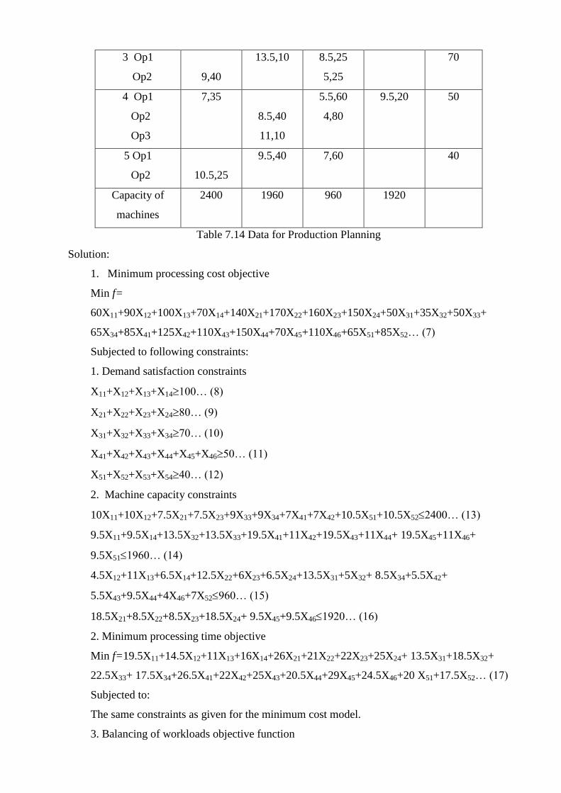
Example 7.5

Consider the manufacturing of five part types on four types of machines. Each part has a number

of operations. The information on demand for each part, capacity available on machines, unit

processing cost, and time for each operation on alternative machines are given in table 7.14.

Develop a production plan using the following models.

1. Minimum processing cost model

2. Minimum processing time model

3. Balancing of workloads model

Parts/Operations

Machines types

M1 M2 M3 M4

Demand

of Parts

1 Op1

Op2

(10,20)*

9.5,40

6.5,30

4.5,70

100

2 Op1

Op2

Op3

7.5,60

6,80

6.5,70

10,60

8.5,20

80

3 Op1

Op2

9,40

13.5,10 8.5,25

5,25

70

4 Op1

Op2

Op3

7,35

8.5,40

11,10

5.5,60

4,80

9.5,20 50

5 Op1

Op2

10.5,25

9.5,40 7,60 40

Capacity of

machines

2400 1960 960 1920

Table 7.14 Data for Production Planning

Solution:

1. Minimum processing cost objective

Min f=

60X11+90X12+100X13+70X14+140X21+170X22+160X23+150X24+50X31+35X32+50X33+

65X34+85X41+125X42+110X43+150X44+70X45+110X46+65X51+85X52… (7)

Subjected to following constraints:

1. Demand satisfaction constraints

X11+X12+X13+X14100… (8)

X21+X22+X23+X2480… (9)

X31+X32+X33+X3470… (10)

X41+X42+X43+X44+X45+X4650… (11)

X51+X52+X53+X5440… (12)

2. Machine capacity constraints

10X11+10X12+7.5X21+7.5X23+9X33+9X34+7X41+7X42+10.5X51+10.5X522400… (13)

9.5X11+9.5X14+13.5X32+13.5X33+19.5X41+11X42+19.5X43+11X44+ 19.5X45+11X46+

9.5X511960… (14)

4.5X12+11X13+6.5X14+12.5X22+6X23+6.5X24+13.5X31+5X32+ 8.5X34+5.5X42+

5.5X43+9.5X44+4X46+7X52960… (15)

18.5X21+8.5X22+8.5X23+18.5X24+ 9.5X45+9.5X461920… (16)

2. Minimum processing time objective

Min f=19.5X11+14.5X12+11X13+16X14+26X21+21X22+22X23+25X24+ 13.5X31+18.5X32+

22.5X33+ 17.5X34+26.5X41+22X42+25X43+20.5X44+29X45+24.5X46+20 X51+17.5X52… (17)

Subjected to:

The same constraints as given for the minimum cost model.

3. Balancing of workloads objective function

Min f=Z3… (18)

Subjected to:

All the constraints given for the first model as well as following extra constraints

Z3- (10X11+10X12+7.5X21+7.5X23+9X33+9X34+7X41+7X42+10.5X51+10.5X52) 0… (19)

Z3-(9.5X11+9.5X14+13.5X32+13.5X33+19.5X41+11X42+19.5X43+11X44+ 19.5X45+11X46+

9.5X51) 0… (20)

Z3-(4.5X12+11X13+6.5X14+12.5X22+6X23+6.5X24+13.5X31+5X32+ 8.5X34+5.5X42+

5.5X43+9.5X44+4X46+7X52) 0… (21)

Z3-(18.5X21+8.5X22+8.5X23+18.5X24+ 9.5X45+9.5X46) 0… (22)

On solving these three models using LINDO (a linear programming package), the results

shown in table 7.15 are obtained.

Parts Process routes Minimum cost

production plan

Minimum

processing time

production plan

Production plan

with balancing of

workloads

Part 1 M1-M2

M1-M3

83

17

100

6

94

Part 2 M4-M1-M4 80 80 80

Part 3 M3-M3

M2-M3

M2-M1

M3-M1

31*

39

60

10

10

Part 4 M1-M2-M2

M1-M3-M2

M4-M2-M2

M4-M3-M2

4*

46*

10

32

8

4

46

Part 5 M2-M1

M3-M1

21

19

40 40

Table 7.15 results of operation allocation and production planning for Example 7.5

SAQ *

1. What are the features of cellular manufacturing system?

2. What are the different steps of an integrated GT and MRP structure

7.7 SUMMARY

This chapter focused on understanding GT concepts and their application in cellular

manufacturing. GT is important because it realizes isolated parts manufacturing by capitalizing

on design and manufacturing similarities among parts. Unfortunately, as manufacturing systems

become larger and the number of parts in these system increases, the ability to apply GT

intuitively to everyday problems decreases. In order to take advantage of GT principles, coding

systems have become essential in industry.

A survey of 53 U.S. companies showed that the use of GT and cellular manufacturing in U.S.

industries have met with success. The benefits reported from these studies include:

reduction in throughput time by 45.6 percent

reduction in work-in-process inventory by 41.4 percent

reduction in material handling by 39.3 percent

reduction in setup time by 32.0 percent

improvement in quality by 29.3 percent

The surveyed companies supported the cellular manufacturing concept, indicating their benefits

exceeding costs (Hyer, N.L., and Wemmerlov, U.).

In this chapter we provided a conceptual understanding of various issues such as classification

and coding systems and planning, and control of cellular manufacturing systems.

7.9 ANSWER TO SAQS Refer the relevant text in this unit for answer to SAQs

7.10 REFERENCES 1. Groover, M..P., 2001. "Automation, Production Systems, and Computer-Integrated

Manufacturing; 2nd Ed". Pearson Education: Singapore.

2. Chu, C.H., and Pan, P., 1998, The use of clustering techniques in cellular formation,

International industrial engineering conference, Orlando, Florida, pp. 495-500.

7.8 KEYWORDS 1. GT Group Technology

2. PFA Production Flow Analysis

3. PF Part family

4. BEA Bond Energy Algorithm

5. ME Measure of effectiveness

3. Ham, I., 1978, Introduction to Group Technology, Technical report, SME, Dearborn,

Michigan.

4. Co, H.C., and Arrar, A., 1988, Configuring cellular manufacturing systems.

International journal of production research, 26, pp 1511-1522.

5. Kusiak, A., 1985, The part families problem in FMSs. Annals of operation research, 3,

pp 279-300.

6. Hyer, N.L., and Wemmerlov, U., 1989, Group technology in the US manufacturing

industry: a survey of current practices, International Journal of Production Planning

Control Research, 27, pp 1287-1304.