UNIT 3 – QUANTITATIVE DATA ANALYSIS - Trent Global · School of the Built Environment 1 UNIT 3...

School of the Built Environment

1

UNIT 3 – QUANTITATIVE DATA

ANALYSIS

• This unit:

– Discusses the tasks of data collection and data manipulation.

– Introduces some statistical concepts


2

DATA MANAGEMENT

• Data management, collection, and interpretation in various forms are basic and regular tasks of the decision making process.

• Distinguish ‘Data’ from ‘Information’ and ‘Knowledge’:

• Data is the raw facts or observations; unprocessed.

• Information are interpreted data which is meaningful and useful

• Knowledge is information with guidance for action.


3

DATA MANAGEMENT

• Data sources could be internal and/or external

• Avoid the GIGO syndrome – quality and integrity of the data are critical for the decision making process

• Major data problems shown in next slide.


4

DATA MANAGEMENT

Problem Typical cause

Data are not correctRaw data were entered inaccuratelyData derived by an individual were generated carelessly

Data are not timelyThe method for generating the data is not rapid enough to meet the need for the data.

Data are not measured or indexed properly

Raw data are gathered according to a logic that is not consistent with the purposes of the analysis

Too many data are needed

A great deal of raw data is needed to calculatecoefficients in a proposed model that is difficultto develop and maintain

Needed data simply do not exist

Required data never existed.


5

COLLECTING DATA

• Data to be collected is linked to the objectives of the decision problem.

• Useful approach to ask a number of questions to link objectives with the data to be collected.

• Questions such as: 'How many?', How much?', 'When?', 'How useful?', 'How expensive?', 'How often?', 'Who?'.


6

DATA CLASSIFICATION

• Data collection process is more successful if the searched data is first classified and understood.

• Data can be broadly classified as quantitative or qualitative.

• Quantitative (numeric) data is easier to collect & analyse; uses mathematical models to manipulate data.

• Qualitative data is non-numeric and more often text describing a situation; Manipulation tools often organise and structure these data relative to one another.


7

DATA COLLECTION PROCESS

• Data can be collected through methods like

– surveys (using questionnaires)

– observation (e.g. using video cameras), and

– soliciting information from experts (e.g. interviews).

• Need to establish data is based on provable facts (certain) or opinions (uncertain).

• If the data is time dependent, critical to identify trends and variation in data.


8

DATA COLLECTION PROCESS

• Data are always a smaller sample used to deduce the characteristics of the larger population.

• To get reliable data, the sample must be:

– Large enough to contain a representative set of items from the population.

– Selected entirely at random to ensure un-biasness.


9

MEASURES OF CENTRAL

TENDENCY

• Measures of central tendency identify the center, or average, of a data set.

• This central point can then be used to represent the typical, or expected, value in the data set.

• Mean, median & mode are common measures of central tendency.


10

MEAN

• To compute the population mean, all the observed values in the population are summed and divided by the number of observations in the population.

– Note that the population mean is unique in that a given population only has one mean.

• The sample mean is the sum of all the values in a sample of a population divided by the number of observations in the sample.

– Sample mean is used to make inferences about the population mean.


11

MEAN

• Properties of mean:

– All data values are considered and included in the arithmetic mean computation.

– A data set has only one arithmetic mean (i.e., the arithmetic mean is unique) .

– The sum of the deviations of each observation in the data set from the mean is always zero.


12

MEAN

• Advantages:

– Concept is familiar to most people and intuitively clear.

– Every data has one and only one mean

• Disadvantages:

– Affected by extreme values

– Tedious to compute

– Unable to compute the mean for a data set that has open ended classes at the either the high or low end of the scale


13

INTERPRETING MEAN

• Be careful when interpreting mean

• Recruiter’s mandate is to recruit pilot with average height of 6 feet; 2 recruits – one 4 feet and the other 8 feet.

• Average class room utilisation is only 20%. What can you conclude from this statement?


14

MEDIAN

• The median is the midpoint of a data set when the data is arranged in ascending or descending order.

• Half the observations lie above the median and half are below

• For even number of observations, median is half-way between the middle 2 numbers.

• Mean can be affected by extreme values. When this occurs, the median is a better measure of central tendency than the mean


15

MEDIAN

• Example: The five-year annualized total returns for five investment managers are 30%, 15%,25%,21% and 23%. Find the median return for the managers.

First, rearrange the returns from highest to lowest:

30% 25% 23% 21% 15%

The return observation half way down from the top or half way up from the bottom is 23%


16

MEDIAN

• Example: Now there is a sixth manager with a return of 28%. What is the median return?

Rearranging the returns gives: 30% 28% 25% 23% 21% 15%

Here the number of observations is even and hence there is no single middle observation.

To find the median take the arithmetic mean of the two middle observations: (25+23)/2.

Thus, the median of the data set is 24%.


17

MEDIAN

• Properties of the median

– The median, like the mean, is unique.

– The median is not affected by extreme values.

– The median can be computed for an open-ended frequency distribution as long as the median does not lie in an open-ended class.


18

MEDIAN

• Advantages:

– Extreme values do not affect the median as strongly as they do the mean.

– Easy to understand and can be calculated form any kind of data

– Can find the median even when data are qualitative descriptions like colour, rather than numbers

• Disadvantages:

– Certain statistical procedures that use the median are more complex than those that use the mean.

– Time consuming to array the data before calculations


19

MODE

• The mode is the value that occurs most frequently in a data set.

• A data set may have more than one mode or even no mode.

• When a distribution has one value that appears most frequently, it is said to be unimodal.

• When a set of data has two or three values that occur most frequently, it is said to be bimodal or trimodal, respectively.


20

MODE

• Advantages:

– The mode can be used for all types of data

– The mode is not affected by extremely large or small values.

– The mode can also be used to measure open-ended data sets.

• Disadvantages:

– For many data sets there may be no value that appears more than once, i.e. no mode.

– On the other hand, some data sets have more than one mode.


21

SKEWNESS

• A distribution is symmetrical if it is shaped identically on both sides of its mean.

• Degree of symmetry (skewness) tells analysts if deviations from the mean are more likely to be positive or negative.


22

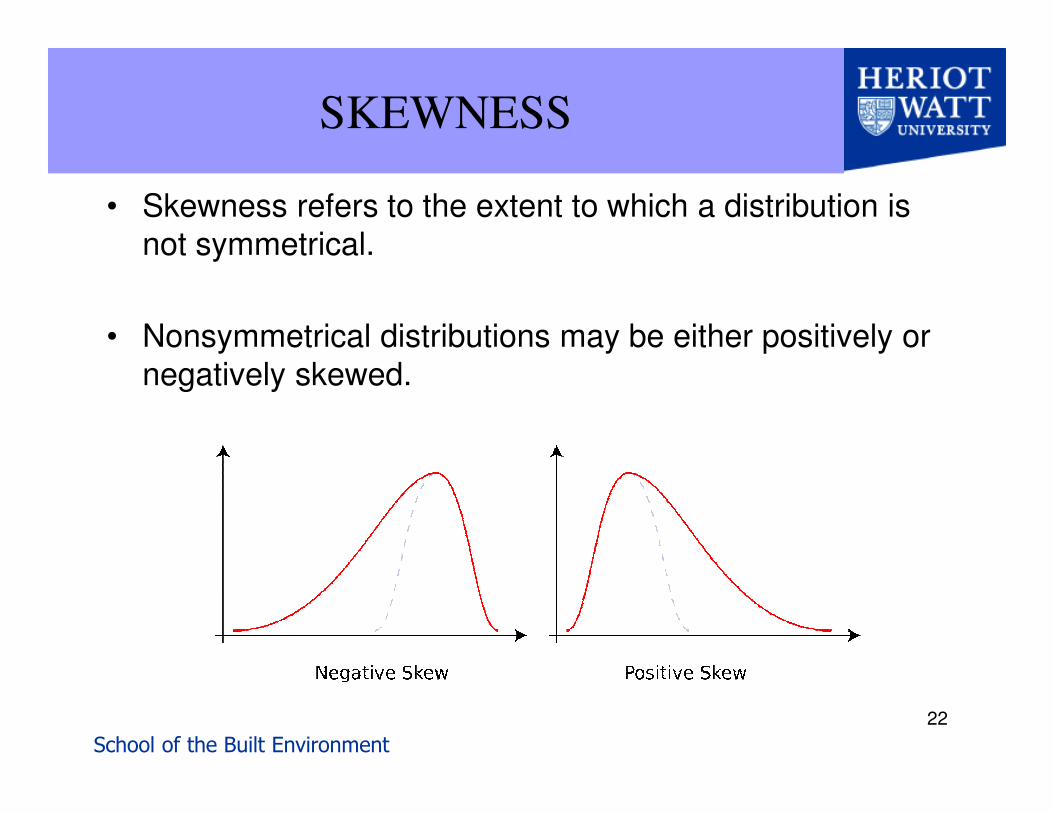
SKEWNESS

• Skewness refers to the extent to which a distribution is not symmetrical.

• Nonsymmetrical distributions may be either positively or negatively skewed.


23

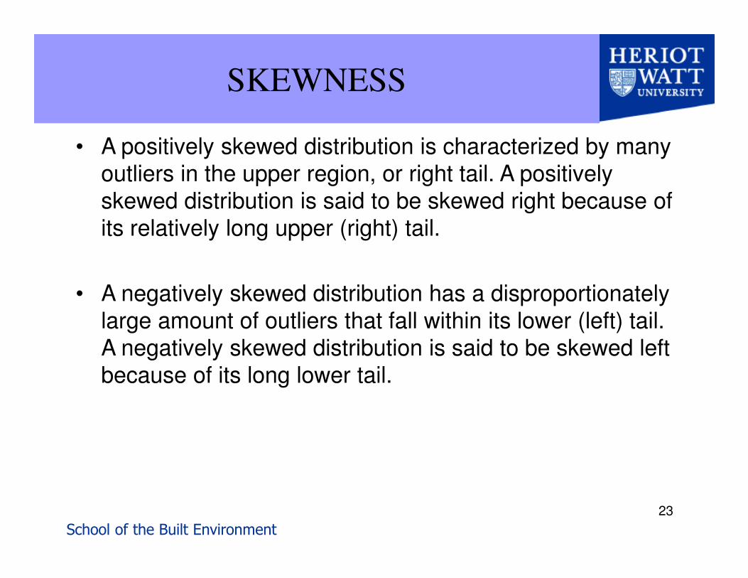
SKEWNESS

• A positively skewed distribution is characterized by many outliers in the upper region, or right tail. A positively skewed distribution is said to be skewed right because of its relatively long upper (right) tail.

• A negatively skewed distribution has a disproportionately large amount of outliers that fall within its lower (left) tail. A negatively skewed distribution is said to be skewed left because of its long lower tail.


24

SKEWNESS

• Skewness affects the location of the mean, median, and mode of a distribution

• When the distribution is skewed, the mean should not be used to represent the data set.

• The median may be best in skewed distributions

• Otherwise there is no universal guidelines for applying the mean, median or mode as the measure of central tendency.


25

SKEWNESS


26

REVIEW QUESTIONS

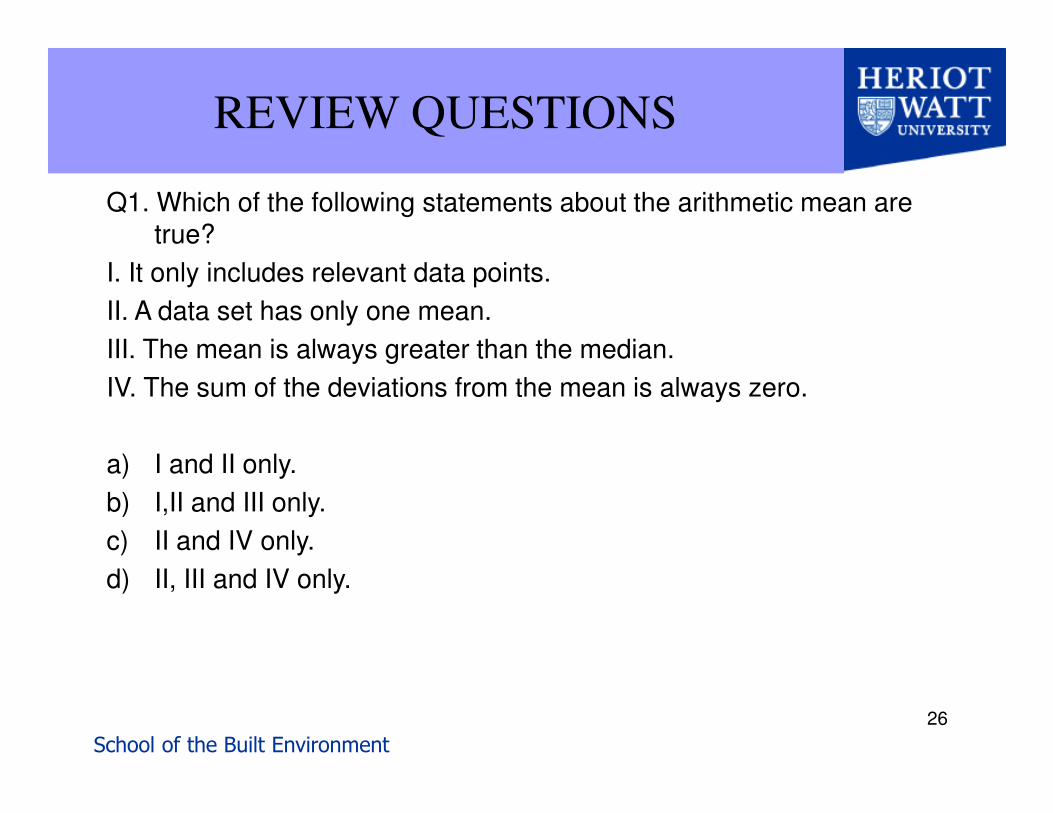
Q1. Which of the following statements about the arithmetic mean are true?

I. It only includes relevant data points.

II. A data set has only one mean.

III. The mean is always greater than the median.

IV. The sum of the deviations from the mean is always zero.

a) I and II only.

b) I,II and III only.

c) II and IV only.

d) II, III and IV only.


27

REVIEW QUESTIONS

Q2. All of the following statements are true except:

a) The mean is influenced by extremely large and small values.

b) The median is a unique number.

c) The median is not affected by extreme values

d) A data set can have only one mode.


28

REVIEW QUESTIONS

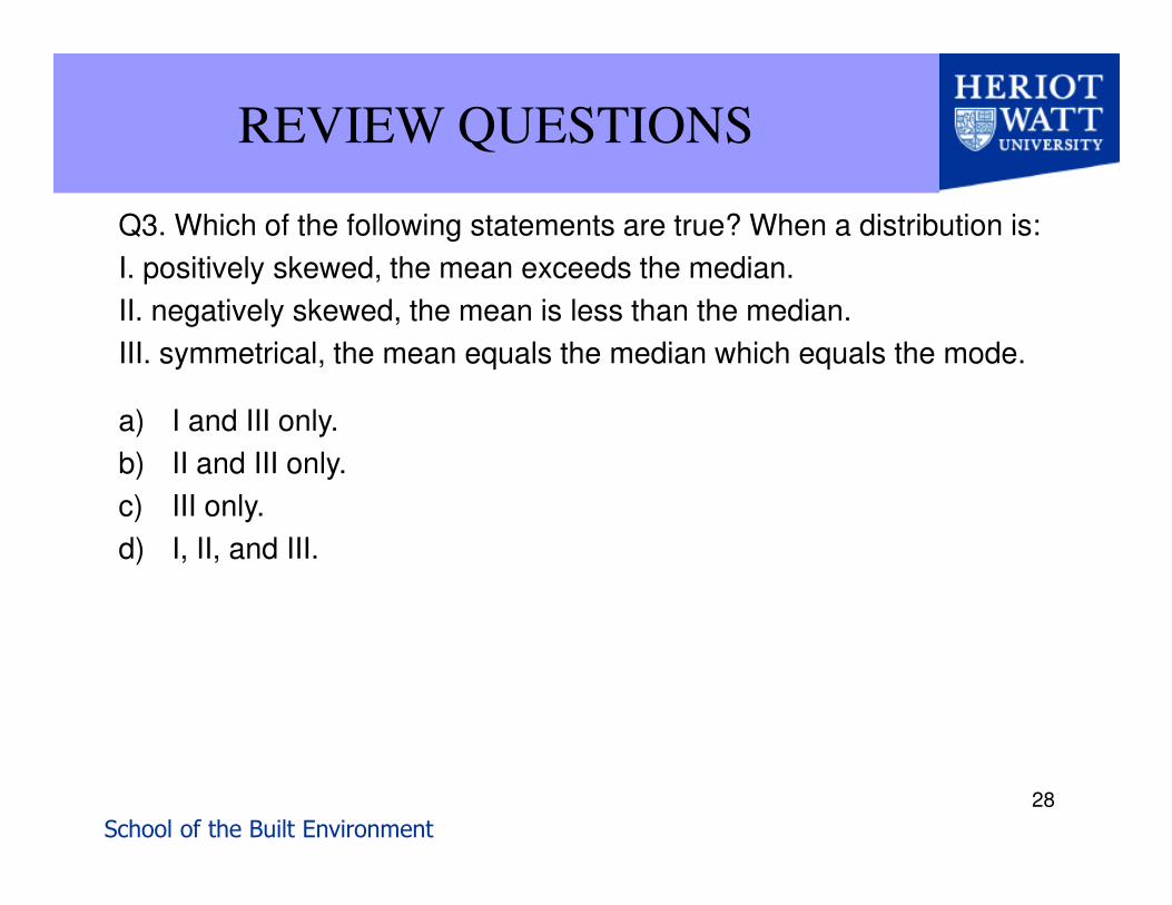
Q3. Which of the following statements are true? When a distribution is:

I. positively skewed, the mean exceeds the median.

II. negatively skewed, the mean is less than the median.

III. symmetrical, the mean equals the median which equals the mode.

a) I and III only.

b) II and III only.

c) III only.

d) I, II, and III.


29

MEASURES OF DISPERSION

• Apart from measuring the central tendency, we can also measure the spread (or variability) of the data series, i.e. Dispersion.

• Why study Dispersion?

– Measures of central tendency pinpoint the center of the data set but don't explain anything about the variability of the individual observations within the data set.

– Studying dispersion enables the analyst to better compare data sets.


30

MEASURES OF DISPERSION

• Dispersion is defined as the variability around the central tendency.

• Two common measures of the degree of spread of a data set is the range and the standard deviation.


31

RANGE

• Range – is the distance between the largest and the smallest value in the data set.

Range = Highest Value - Lowest Value

Example: The five-year annualized total returns for five investment managers are 30%,12%, 25%, 20% and 23%. What is the range of the data?

Range: 30 – 12 = 18%

• The problem with range as a measure is that it is vulnerable to extreme values


32

STANDARD DEVIATION

• The most common measure of dispersion accompanying the mean of a distribution is the standard deviation or variance

• The variance is defined as the average of the squared deviations from the mean.

• Population variance is calculated as follows:


33

STANDARD DEVIATION

• Sample variance is the dispersion measure when we are evaluating a sample of n observations from a population

• The major problem with using the variance is the difficulty interpreting it. Why? The variance unlike the mean is in terms of units squared


34

STANDARD DEVIATION

• Problem is mitigated through the use of the standard deviation.

• Standard deviation is the square root of the variance.

• The standard deviation is commonly used to compare the spread in two or more sets of data.


35

STANDARD DEVIATION

• For example, the return per $100 invested of plants A & B is shown below

Plant A Plant B

Mean $15 $15

Standard Dev $10 $15

• Since Plant A's returns are more tightly grouped than those at Plant B, one could conclude that the mean return of Plant A's is a more reliable measure than Plant B's mean


36

REVIEW QUESTIONS

Q1 Which one of the following statements is false?

a) The measurement units of the standard deviation are always the same as those of the original data

b) The standard deviation is the square root of the variance

c) The range is not greatly influenced by extremely large or small data values

d) The variance is difficult to interpret because it is expressed in square units


37

NORMAL DISTRIBUTION

• Characteristics of normal distributions:

– The normal curve is bell-shaped with a single peak at the exact center of the distribution.

– The arithmetic mean, median, and mode are equal. Half of the area under a normal curve lies above the mean and half below the mean.

– The normal curve can be completely defined by its mean and standard deviation.


38

NORMAL DISTRIBUTION

• Characteristics of normal distributions:

– The normal distribution is symmetrical about its mean.

– The normal curve falls off smoothly in either direction from the central value.

– The normal curve is asymptotic to the X-axis in both directions, i.e. the tails go on to infinity in both directions as they get closer and closer to the axis


39

NORMAL DISTRIBUTION

• Why do we use normal distributions? Normaldistributions are often used to represent randomvariables whose distributions are not known.


40

NORMAL DISTRIBUTION

• Normal distributions come in many sizes and shapes. For example:

– The three normal curves below have the same mean but different standard deviations


41

NORMAL DISTRIBUTION

– The two normal curves below have the same standard deviations but different means

• The number of different normal curves are unlimited


42

AREA UNDER THE NORMAL

CURVE

• The proportions under a normal curve are stable. The area under the normal curve is used to represent probabilities

68.2% of observations are within±1σ of µ

95.4% of observations are within ±2σ of µ

99.7% of observations are within ±3σ of µ


43

NORMAL DISTRIBUTION

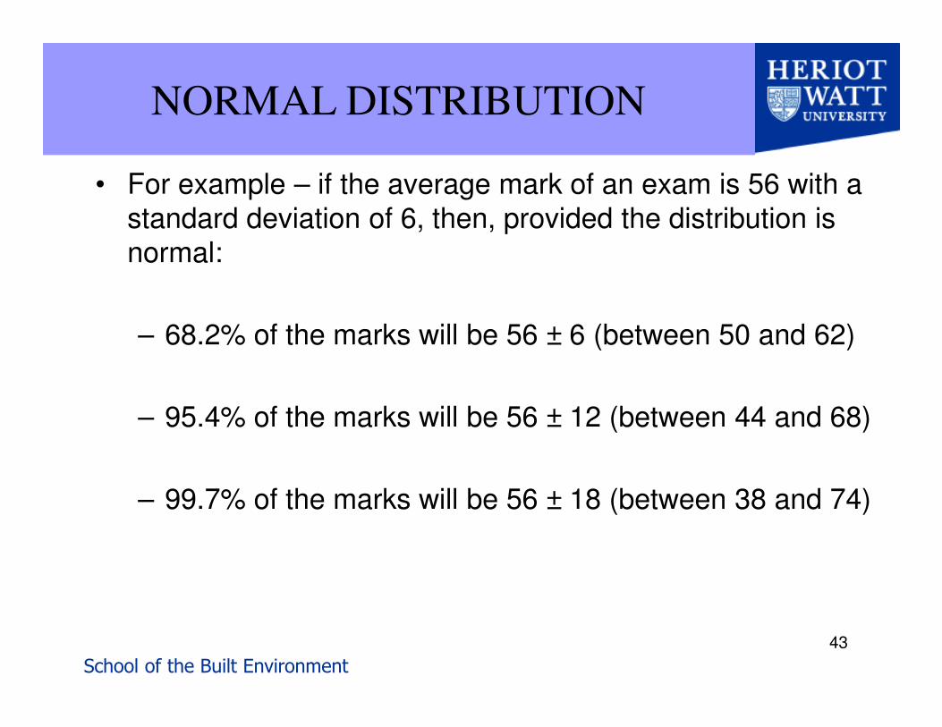
• For example – if the average mark of an exam is 56 with a standard deviation of 6, then, provided the distribution is normal:

– 68.2% of the marks will be 56 ± 6 (between 50 and 62)




44

REGRESSION ANALYSIS

• Regression analysis is a technique to model and analyse numerical data to:

– test whether there is a dependent relationship between an outcome (dependent) variable and a predictor (independent) variable; and

– the strength of dependence.


45

REGRESSION ANALYSIS

• Tests the relationship between a dependent variable (Y) and one or more independent variables (X).

• Helps us understand how the typical value of the dependent variable (Y) changes when any one of the independent variables (X) is varied.


46

REGRESSION ANALYSIS

• Regression models predict a value of the dependent variable given known values of the independent variables.

• Prediction within the range of values is known as interpolation.

• Prediction outside the range of the data is known as extrapolation, which is more risky.


47

REGRESSION ANALYSIS

• Different type of regression: linear, exponential, multiple

• Linear regression

– assumes that the bestrelationship between thedependent and independentvariables is linear.

– It produces the slope of a line thatbest fits a single set of data.

– By following this line forward intime, an estimate for future datacan be produced.


48

REGRESSION ANALYSIS

• Exponential regression

– Assumes that the bestrelationship between thedependent and independentvariables is exponential.

– It produces an exponentialcurve that best fits a set ofdata that does not changelinearly with time.


49

REGRESSION ANALYSIS

• Multiple regression

– is an extension of simple linear regression.

– It is used when we want to predict the value of a variable based onthe value of two or more other variables (i.e. use many X to predictY).


50

REGRESSION ANALYSIS

• A relationship may exists between X and Y variable and you may want to develop an equation that expresses this relationship so that you can forecast the value of Y given an estimate of what X will be.

• This involves drawing a straight line through the data points in the scatter diagram. This line is called the regression line.

• Before we dwell into the regression line, we need to first understand the properties of a straight line.


51

FORMULA FOR STRAIGHT A LINE:

Y axis

X axis

-10 -5 0 5 10

Y = a + bX

Y= 3 -1.5X

Y= -9 - 1.5X

Y=14 - 1.5X

♦ The “constant” or “intercept” (a)

– Determines where the line intersects the Y-axis

– If a increases (decreases), the line moves up (down)

-9

3

14


52


Y axis

X axis

-10 -5 0 5 10

20

10

-10

-20

Y=3-1.5X

Y=3+.2X

The slope (b) determines the steepness of the line

When b is positive, the line is upwards sloppingWhen b is negative, the line is downwards slopping


53


-10 -5 0 5 10

20

10

-10

-20

Y=3+3X

The slope tells you how

many points Y will

increase for any single

point increase in X

Change in X =5

Change in Y=15

b = 15/5 = 3

The slope (b) is the ratio of change in Y to change in X


54

ESTIMATING THE

REGRESSION LINE

• How then do you fit a regression line through the scatter diagram?

-4 -2 0 2 4

4

2

-2

-4Y=1.5-1X

• A poor estimation (large error)


55

ESTIMATING THE

REGRESSION LINE

-4 -2 0 2 4

4

2

-2

-4

Y=2+.5X

• Better estimation (small error)


56

ESTIMATING THE

REGRESSION LINE

• The regression’s line of best fit is established with the least square principle.

• Each distance of a point from the line can be calculated.

• The least squares method places a line through a set of points such that the sum of the squares of the differences between each point and the line is a minimum.


57

LINEAR REGRESSION

• The least squares method specifies a straight line (ie linear relationship) between X and Y.

• The equation for a straight line is:

Y = a + bX

where Y = Dependent variable

X = Independent variable

a = Y-intercept

b = slope of the line

• a & b are the unknown parameters to be estimated. Once a & b are estimated, you can use them to project Y given X.


58

LINEAR REGRESSION


59

LINEAR REGRESSION

• Example - Given the following data, estimate the regressionline.


60

LINEAR REGRESSION

• Solution


61

LINEAR REGRESSION

• Equation is: Income = -7276.19 + 1390.476 experience

• Interpretation:

– When there is no experience, income is -7276.19

– Every year of experience gives an income of 1390.476.

– If you have 13 years experience, you can predict theincome to be = -7276.13 + 13(1390.476) = 10800


62

R-SQUARE

• Even the “best” regression line misses data points. We still have some errors.

• How good is our line at summarizing the relationship between two variables?

– Do we have a lot of error? Or only a little? (i.e., the line closely estimates data points)

• The R-Square statistic help us to answer these questions


63

R-SQUARE

• The R-Square statistic is computed as follows:

• Q: What is R-square if the line is perfect?

• Answer: R-square = 1.00

• Q: What is R-square if the line is NO HELP in estimating points? (i.e. lots of error)

• Answer: R-square is zero

VariationTotal

VariationExplainedRYX

_

_2=


64

R-SQUARE

SPSS OutputModel Summary

.566a .320 .306 8.926

Model1

R R SquareAdjustedR Square

Std. Error ofthe Estimate

Predictors: (Constant), Povertya.

ANOVAb

1839.069 1 1839.069 23.081 .000a

3904.252 49 79.679

5743.322 50

Regression

Residual

Total

Model1

Sum ofSquares df Mean Square F Sig.

Predictors: (Constant), Povertya.

Dependent Variable: CrimeRateb.

The R-Square

indicate how

well the line

summarizes

the data, or

how much of

the variance

can be

explained by

the model.


65

PROPERTIES OF R-SQUARE

• R2 ranges from 0 to 1

– 1 indicates that perfect prediction of Y by X

– 0 indicates that the line explains no variance in Y

• Tells us the proportion of all variance in Y that is explained as a linear function of X

– It measures “how good” our line is at predicting Y (goodness of fit)

• The R2 indicates how well variables account for variation in Y (explanatory power)

– R-square=0.32 means 32% of variance in crime rate (Y) is explained by poverty rate (X)


66

INTERPRETING R-SQUARE

• R2 is often used as an overall indicator of the “success” of a regression model

• Higher R2 is considered “better” than lower


67

REVIEW QUESTIONS

Q1 All of the following statements are true except:

a The dependent variable is plotted on the X

b. The independent variable is assumed to influence the dependent variable.

c. The variable that is acted upon is called the dependent variable.

d. The variable plotted on the X-axis motivates the variable plotted on the Y-axis


68

REVIEW QUESTIONS

Q2 Which one of the following statements about regression lines is true?

a. the alpha and beta coefficient must be positive

b. the greater the alpha coefficient the steeper the regression line

c. given an alpha of 2 and beta of 3, if Y were 1 the X would be 5

d. given an alpha of 2 and beta of 3, if X were 1 the Y would be 5


69

CLASS EXERCISE 1

• The table below shows data collected by a contractor aboutcosts and durations of projects. Determine the linearrelationship between cost and duration and estimate theduration of a project with the total cost of $210,000

Projects 1 2 3 4 5 6

Cost, $ 100 115 120 180 230 300

Duration (months)

8 10 14 18 24 30


70

CLASS EXERCISE 2

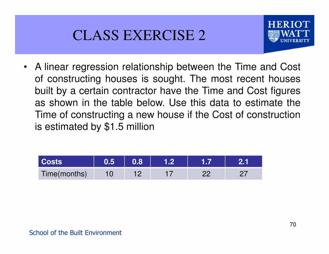
• A linear regression relationship between the Time and Costof constructing houses is sought. The most recent housesbuilt by a certain contractor have the Time and Cost figuresas shown in the table below. Use this data to estimate theTime of constructing a new house if the Cost of constructionis estimated by $1.5 million

Costs 0.5 0.8 1.2 1.7 2.1

Time(months) 10 12 17 22 27


71

CLASS EXERCISE 3

• A study was conducted to establish a linear regressionrelationship between the GDP and the budget spent onpublic construction projects. The data for the last 5 years isassumed as shown in the table below. Use this data toestimate the public spending on construction, if the GDP isdropped to $1.7 trillion

GDP (trillion $) 1.2 1.5 1.8 2.1 2.4

Public construction budget ($ billion)

10 12 17 22 27


72

CHI SQUARE TEST

• The chi-squared test is a statistical test used to examine differences with categorical variables presented in a table format.

• It is mainly used to estimate whether two random variables are independent or not. E.g. are income and education level related? Is price related to quality?

• If two categorical variables are correlated, their values tend to move together; either in the same direction or in the opposite.


73

CHI SQUARE TEST

• A hypothesis is usually set to be tested:

• A null hypothesis (H0) of "no difference" or “no relationship” between two variables is first set

• The alternate hypothesis (H1) of “there is difference” or “there is a relationship” will be accepted if H0 is rejected.

• To test the null hypothesis, we must compare the frequencies that were observed with the frequencies we would expect if the null hypothesis is true.


74

CHI SQUARE TEST

• Expected frequency for each cell of the table can be calculated using the following formula


75

CHI SQUARE TEST

• If the sets of observed and expected frequencies are nearly alike, we can accept the null hypothesis.

• If there is a large difference between these frequencies, we may reject the null hypothesis and accept the alternate hypothesis that there are significant differences

• To test for any significant differences, we calculate the Chi-Square statistic:


76

CHI SQUARE TEST

• Chi-Square statistic:

• If this chi-square value is large, it indicates a substantial difference between the observed and expected values.

• A chi-square value of zero indicates that the observed frequencies exactly match the expected frequencies.

• The value of chi-square can never be negative


77

CHI SQUARE TEST

• If Ho is true, then the sampling distribution of the chi-square statistic can be approximated by a chi-square distribution

• There is a different chi-square distribution for each different number of degrees of freedom.


78

CHI SQUARE TEST

• Figure below indicates the 3 different chi-square distributions that would correspond to 1, 5, and 10 degrees of freedom.

• As the number of degrees of freedom increases, the curve rapidly becomes more symmetrical, at which point the distribution can be approximated by the normal distribution.


79

CHI SQUARE TEST

• The number of degrees of freedom is calculated by applying the equation below:

• Example – 3X3 table below has (4-1)(3-1)=6 degrees of freedom

Annual income <20,000 20,001 – 50,000 >50,001

PSLE 15 30 20

GCE O 34 100 120

GCE A 55 150 100

University 75 111 123


80

CHI SQUARE TEST

• Using the chi-square table (a statistical table), check up the value corresponding to calculated degrees of freedom and desired level of significance.

• If the calculated chi-square statistic is less that the values given in the statistical table, then we accept the null hypothesis.


81

CHI SQUARE TEST

• Example – 2 types of materials (material ‘a’ and material ‘b’)are used for the construction of 2 types of houses (Privateand Social houses). Table below shows the number of timeseach material was selected for each type of houses.Determine if the choice of material is independent of thetype houses at 5% significance level.

Private houses Social houses Total

Material ‘a’ 46 71 117

Material ‘b’ 37 83 120

Total 83 154 237


82

CHI SQUARE TEST

1. Establish hypothesis

H0: There is no relationship between choice of material and type of houses

H1: The choice of material is dependent on the type of houses


83

CHI SQUARE TEST

2. Calculate the expected frequency

Observed frequencyPte house Social house Total

Material "a" 46 71 117Material "b" 37 83 120

83 154 237

Expected frequencyPte house Social house Total

Material "a" 40.97 76.03 117Material "b" 42.03 77.97 120

83 154 237


84

CHI SQUARE TEST

3. Calculate the chi-square statistic

Fo Fe Fo-Fe (Fo-Fe)2 (Fo-Fe)2 / Fe46 40.97 5.03 25.30 0.6237 42.03 -5.03 25.30 0.6071 76.03 -5.03 25.30 0.3383 77.97 5.03 25.30 0.32

1.88


85

CHI SQUARE TEST

4. Assess significance level

Degree of freedom = (2-1)(2-1) = 1.

With 1 degree of freedom at 5% significance level, the critical chi-square value (from chi-square table) is 3.84.

Calculated chi-square statistic of 1.88 is < 3.84. Thus null hypothesis is not rejected.

As such the choice of materials and type of houses are independent.


86

CLASS EXERCISE 4

• A contractor company employs three quantity surveyors (A,B & C). If errors in estimation or measurement occur duringor after projects, the surveyor’s report should be reviewedby a consultant. The company examines the record of the 3surveyors. Surveyor A had 6 out of her last 47 reportsreviewed, Surveyor B had 4 out of his last 72 reportsreviewed and Surveyor C had 14 out of his last 41 reportsreviewed. Test, at the 5% significance level, whether theproportion of reports reviewed is independent of thesurveyor.


87

CLASS EXERCISE 5

The residents in 3 different areas of Edinburgh city were askedwhether they would prefer the local authority to spend ongeneral road improvement or on improving public transport.The replies are shown in the table below.

Test, at the 5% significance level, whether the proportion ofthe residents’ preference is independent of the area.

Area A Area B Area C

Improves roads 80 48 26

Improves public transport

24 36 38


88

T-TEST

• T-test is a technique for comparing the means of two samples.

• In simple terms, the t-test compares the actual difference between two means in relation to the variation in the data (expressed as the standard deviation of the difference between the means).

• One of the advantages of the t-test is that it can be applied to a relatively small number of cases. It was specifically designed to evaluate statistical differences for samples of 30 or less.


89

T-TEST

• It is used to evaluate 2 kinds of hypothesis:

1. The one-sample t-test, in which the mean score of a sample (observed average) is compared to a known value, usually the population mean (expected average) with an adjustment for the number of cases in the sample and the standard deviation of the sample average.

2. The two-sample t-test, where the means of two groups are compared to each other to see if they are equal.


90

ONE SAMPLE T-TEST

• It was found that labours with low skills have lower level of productivity than those of high skills. Assuming the industry average level of productivity of highly skilled labours is measured as approximately 3300 hours/year, the average for low skilled labours is 2800 hours/year.

• Recently, a new training program to improve the skills of labours has been organised by a company. 25 low skilled labours participated in this program. Data drawn from the program revealed that the level of productivity had improved to 3075 hours/year, with a standard deviation of 300 hours/year. The question is: has the program been effective at improving the productivity levels of low skilled labours?


91

ONE SAMPLE T-TEST

• With training, the productivity has improved to 3075 hours/year compared to the industrial average of 2800. Is this difference significant or is it due to chance (i.e. sampling error?)

• Null hypothesis: there that no difference has been observed between the level of productivity of labours who participated in the program and those who did not

• Alternative hypothesis: there is a significant difference between the observed mean of productivity for program labours and the expected mean of productivity for low skilled labours.


92

ONE SAMPLE T-TEST


93

ONE SAMPLE T-TEST

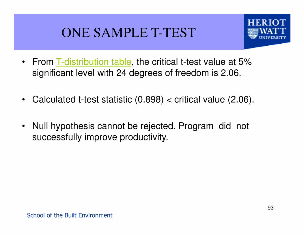
• From T-distribution table, the critical t-test value at 5% significant level with 24 degrees of freedom is 2.06.

• Calculated t-test statistic (0.898) < critical value (2.06).

• Null hypothesis cannot be rejected. Program did not successfully improve productivity.


94

TWO SAMPLE T-TEST

• The steps are similar to those of the one-sample test.

• From the earlier example, rather than comparing the productivity level of the low skilled labours to the industry average, the exercise will compare the productivity level of labours who participated in the program with the labours of a group who did not.

• A comparison of this sort is very common to evaluate the effects of some intervention such as program or treatment.


95

TWO SAMPLE T-TEST

• A group receiving the treatment or training (treatment / trained group) is to be evaluated against those who do not (control or comparison group).

• The following information is given:

Trained group Control group

Average Productivity level (hours/year) 3100 2750

SD 420 425

n 75 75


96

TWO SAMPLE T-TEST

• Null hypothesis: there is no difference between the mean of the productivity level of the group participated in the training program and the mean of those who did not.

• Alternative hypothesis: there is difference between the mean productivity level of the group participated in the training and the mean of those who did not.


97

TWO SAMPLE T-TEST

• The t-test statistic is calculated as:


98

TWO SAMPLE T-TEST

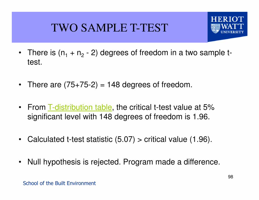
• There is (n1 + n2 - 2) degrees of freedom in a two sample t-test.

• There are (75+75-2) = 148 degrees of freedom.

• From T-distribution table, the critical t-test value at 5% significant level with 148 degrees of freedom is 1.96.

• Calculated t-test statistic (5.07) > critical value (1.96).

• Null hypothesis is rejected. Program made a difference.


99

CLASS EXERCISE 6

A program to reform the financial profile of a constructioncompany has been adopted by an SME contractor. Theprogram includes certain policies to procure and price projectswith other sub-contractors and material suppliers. The adoptedprogram has been applied to 5 projects by the SME contractor,after which the turnover of the SME has improved to$8.5M/year with a standard deviation of $0.5M/year. The dataavailable from industry shows that the average turnover of anSME contractor is $10M/year. The average turnover of theSME contractor (before applying the new program) was$8M/year. The question is: has the program been effective atimproving the turnover of this SME contractor to the industrylevel?


100

CLASS EXERCISE 7

The head of the English department is interested in thedifference in writing scores between freshman Englishstudents who are taught by different teachers. The incomingfreshmen are randomly assigned to one of two Englishteachers and are given a standardized writing test after thefirst semester. We take a sample of eight students from oneclass and nine from the other. Is there a difference inachievement on the writing test between the two classes? Testat 5% significant level.

The data from the two classes is shown in next slide:


101

CLASS EXERCISE 7


102

THE END

Any questions?


103

MEASUREMENT

• Variables are things that we measure, control, or manipulate in research

• A category variable has 2 or more classifications. Eg sex (male, female), hair color (black, blond, brunette, red etc)

• A nominal variable is one that has two or more classification but there is no intrinsic ordering to the classifications. Eg hair colour.

• An ordinal variable is a categorical variable with a clear ordering of the classifications. Eg income level (high, medium, low)

Variables

Category Quantity

Discrete ContinuousNominal

(categories)

Ordinal(ordered

Categories)

Different types of variable


104

MEASUREMENT

• Quantity variables have the value of numbers which are available for arithmetic. Eg number of houses, price etc.

• Discrete variables can only take on a finite number of values. For example, responses to a five-point rating scale can only take on the values 1, 2, 3, 4, and 5. The variable cannot have the value 1.7. Equal distance between values.

• Continuous variables can take on an infinite number of possible values. An e.g. would be a person's height which can take on any value.

Different types of variable

Variables

Category Quantity

Discrete ContinuousNominal

(categories)

Ordinal(ordered

Categories)


105

STATING HYPOTHESIS

• The Null Hypothesis (H0) is astatement about the value of apopulation parameter

– Always have equality sign: =, ≥ or ≤

• The Alternate Hypothesis (H1) is thestatement that will be accepted if thesample data provides evidencerepudiating the null hypothesis.

– Always have inequality sign: ≠, < or >

• Must be mutually exclusive & exhaustive


106

STATING HYPOTHESIS

• Illustration: Test that the population mean is not 3.

• Steps:

– State the question statistically: µ ≠ 3

– State the opposite statistically: µ = 3

– Select the null hypothesis: µ = 3 (Tip: it has the equality sign.)

– Alternate hypothesis: µ ≠ 3


107

WHAT ARE THE HYPOTHESES?

1. Is the population average amount of TV viewed 12 hours?

2. Is the average cost per hat less than or equal to $20?

3. Is the average amount spent in the bookstore greater than $24?


108


1. Is the population average amount of TV viewed 12 hours?

– State the question statistically: µ = 12

– State the opposite statistically: µ ≠ 12

– Select the null hypothesis: µ = 12 (It has the equality sign.)

– Alternate hypothesis: µ ≠ 12


109


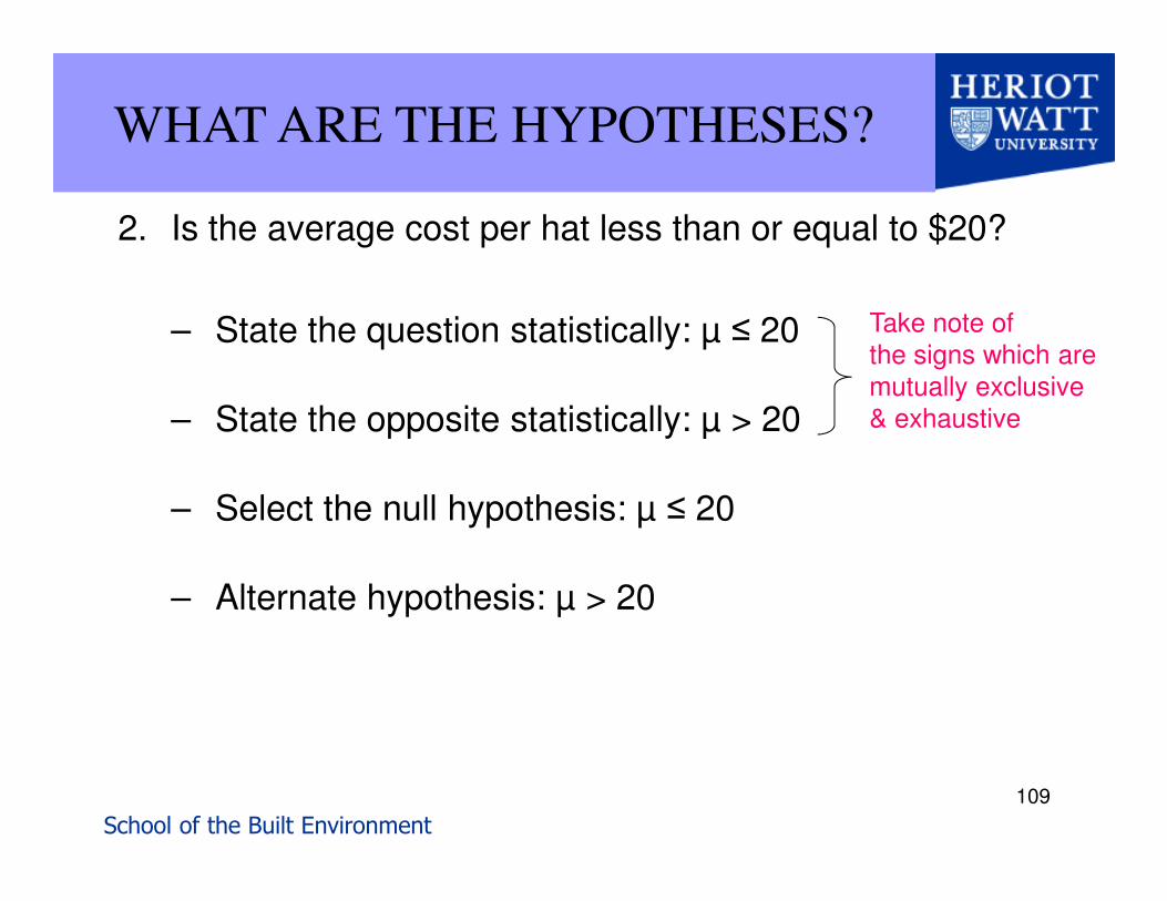
2. Is the average cost per hat less than or equal to $20?

– State the question statistically: µ ≤ 20

– State the opposite statistically: µ > 20

– Select the null hypothesis: µ ≤ 20

– Alternate hypothesis: µ > 20

Take note of the signs which are mutually exclusive & exhaustive


110


3. Is the average amount spent in the bookstore greater than $24?

– State the question statistically: µ > 24

– State the opposite statistically: µ ≤ 24

– Select the null hypothesis: µ ≤ 24

– Alternate hypothesis: µ > 24


111

• Many.

CHI-SQ TABLE


112

LEVEL OF SIGNIFICANCE

• Defined as the probability of rejecting the null hypothesis when it is actually true.

• The significance level is called the level of risk or α and is usually set at 5% or 1%.

– Selected by researcher at start


113

T-Distribution


114

THE END

Any questions?

UNIT 3 – QUANTITATIVE DATA ANALYSIS - Trent Global · School of the Built Environment 1 UNIT 3...

Documents

Transcript of UNIT 3 – QUANTITATIVE DATA ANALYSIS - Trent Global · School of the Built Environment 1 UNIT 3...