Unit 20: Applications and interpretations of wave mechanics

1 Making predictions with quantum mechanics

Perhaps the most significant scientific revolution since the time of Newton, began at around the turn of the twentieth century

and peaked in the mid-1920s, with the advent of Schrödinger’s formulation of quantum mechanics. The need for a

revolutionary theory of microscopic nature began to be recognised as the results of experimental atomic physics accreted

into a body of evidence which, scientists eventually realised, undermined many of the basic ideas of classical mechanics.

The challenge to classical mechanics could hardly have been more formidable, for the world of classical mechanics is

deterministic. Classical mechanics supposes that, while the mathematical difficulties are often insurmountable, it is in

principle possible, given sufficient information about the present, to predict the future exactly, that is, to predict the progress of

any experiment with absolute certainty. The evidence from atomic physics implied that this was not true of microscopic

nature. In microscopic nature, identical conditions do not produce identical results.

The theory that embraces the indeterminism of the microscopic world is called quantum mechanics and is the main subject

of this Unit. It provides an intellectually satisfying and coherent framework for solving problems in atomic physics (among

other areas), and hence for understanding the behaviour of matter. The theory of quantum mechanics reveals many new,

exciting and unforeseen effects.

In the previous Unit, you saw that electromagnetic radiation and matter exhibit what is often termed wave–particle duality: in

different circumstances, either a wave model or a particle model may be required to account for some observed aspect of

their behaviour. In classical physics these two models are contradictory. In quantum physics they must somehow be brought

together to provide a single self-consistent description. This is what quantum mechanics achieves.

You will realise as you read this Unit that the study of quantum mechanics draws on many ideas and principles from other

parts of physics. In particular, we shall make use of concepts from Newtonian mechanics, electricity and magnetism, and the

study of waves. It is, however, very important to note at the outset that the laws of quantum mechanics are completely

different from the laws of classical mechanics. And, whereas classical mechanics is based on intuitively reasonable ideas,

quantum-mechanical ideas are very unintuitive and may therefore appear somewhat harder to grasp. Nevertheless, it is

essential to come to grips with these new ideas in order to understand the behaviour of matter at the atomic level.

2 The Schrödinger equation

Much of the credit for laying the foundations of a proper theoretical understanding of atomic matter belongs to the Austrian

physicist Erwin Schrödinger (Figure 1). Schrödinger used de Broglie’s ideas as the starting point for the systematic

development of wave mechanics, one of the earliest and simplest formulations of quantum mechanics. (Note that there are

several mathematically equivalent ways of expressing the principles of quantum mechanics; wave mechanics is one of them.)

In developing wave mechanics, Schrödinger went far beyond de Broglie’s simple association of waves and particles. In

particular, in 1926, Schrödinger published an equation that did for quantum mechanics what Newton’s laws of motion had

done for classical mechanics nearly 250 years earlier. This tremendous step forward in our understanding of Nature is the

main subject of this section.

Figure 1 Erwin Schrödinger.

Show transcriptDownloadAudio 1 Short biography of

Erwin Schrödinger.

In Schrödinger’s theory, probability waves arise as variations in a quantity (the upper case, Greek letter psi) that is referred

to as a wavefunction. In Schrödinger’s wave-mechanical description of the behaviour of a particle, is a function of position

and time, so it may be written as . At this stage it’s best to think of as the analogue of the quantities that vary in

other types of wave motion — the displacement of a plucked string from its equilibrium position for example, or, in the case

of an electromagnetic wave, the electric field or the magnetic field , both of which oscillate as the wave

propagates. It is not possible to ascribe any direct physical meaning to the quantity , but, as will be explained later,

wavefunctions can be related to probabilities of measured results, just as the amplitudes of probability waves were in

Section 4.5 of Unit 19.

The wavefunction that describes the behaviour of any particular quantum system is found by solving the appropriate form

of Schrödinger’s equation. In order to keep the mathematics at an appropriate level for this Module, we will restrict our study

of quantum mechanics to sufficiently simple situations, where it is possible to develop an insight into the subject. In particular,

we shall mostly restrict the discussion to just one dimension — usually taken to be the -direction. Even so, you should still

be able to see how Schrödinger’s equation provides a description of particle behaviour in terms of a wavefunction ,

and why this description leads naturally to the quantisation of the energy of particles in certain circumstances.

2.1 Travelling and standing waves

In what follows we shall be concerned with essentially two types of waves, introduced in Section 3 of Unit 14 and Section 4 of

Unit 14: travelling waves and standing waves. A travelling wave is characterised by the fact that it is associated with some

particular direction of propagation, and the profile of the wave moves in that direction as time progresses. In contrast, a

standing wave has no direction of propagation, though its profile does change with time. In the case of a standing wave there

are generally several fixed points called nodes, at which the displacement from equilibrium is zero at all times; between the

nodes the displacement increases and decreases periodically as each part of the wave oscillates about its equilibrium

position. A sequence of snapshots of a travelling wave and a standing wave are shown in Figure 2. Both waves have the

same amplitude and period, and both have the same wavelength .

Now, as you know, waves can have any wavelength when they are free to propagate over an effectively infinite distance —

an infinitely long string for example, or a very large expanse of water. On the other hand, when a wave is confined in a

restricted space — a finite length of string fixed at both ends for example, or an organ pipe, the wave may take the form of

a standing wave with a wavelength determined by the size of the system (see Figure 2).

Figure 2 Travelling waves and standing waves. (a) A sequence of

snapshots of a travelling wave on an infinitely long string. (b) A

similar sequence of snapshots of a standing wave, of wavelength

, on a finite string of length with fixed endpoints.

Similar behaviour occurs in situations described by quantum mechanics: when a particle is free to move over an unrestricted

region of space, its wavefunction is characterised by the (de Broglie) wavelength , which can take any value, since the

magnitude of the momentum is unrestricted. If, however, the particle is confined in some way, by being trapped in a ‘box’ of

some sort, its wavefunction will involve standing waves of a particular wavelength and there will be corresponding restrictions

on its movement and energy.

Whether or not a particle is ‘free’ or ‘confined’ is determined by the energy of the particle, and by the way its potential energy

varies throughout the region in which the particle might be found. The potential energy function introduced in Section 3 of

Unit 5 of a particle, , is simply the expression that relates the particle’s potential energy, , to its position in

space, . If the particle’s motion is restricted to the -direction then it can simply be written . Not surprisingly, the

potential energy function turns out to be a very important quantity in Schrödinger’s equation. By including it in the equation

we can be assured that the equation takes a form that is relevant to the problem being considered, whatever that might be.

Because of this, before we go on to look at Schrödinger’s equation in detail, it is worth considering what we mean by ‘free’ or

‘confined’ in terms of the potential energy of a particle.

2.2 Free and confined particles

In everyday terms, a particle is confined, or bound, within a certain region if there is some sort of barrier preventing its escape

from that region. Think of a squash ball bouncing about in a squash court. The ball has quite a lot of kinetic energy but it will

never be able to break through the barrier constituted by the walls that confine it. The ball would be destroyed before it could

acquire enough energy to penetrate any wall of the court. If the walls were more flimsy however, it is possible to imagine that

the ball might acquire enough kinetic energy to break through and escape. If its energy is less than this threshold the ball will

be confined, if it is greater then it will not be confined.

In more technical terms, a particle is confined, otherwise known as a bound particle, if its total energy is insufficient to allow

it to overcome the barrier of potential energy that is surrounding it. If the particle’s total energy is greater than the potential

energy barrier, the particle can escape and is then said to be an unbound particle. An unbound particle for which the

potential energy may be taken to be constant everywhere is said to be a free particle: if is constant, the particle has no

forces acting on it.

Let us think about a concrete example, using the form of potential energy that is probably most familiar to you — gravitational

potential energy (you may want to check Section 3.4 of Unit 5 to remind yourself). At the surface of the Earth, we can confine

an object in a gravitational ‘potential well’ simply by digging a hole (or well) and dropping the object in with insufficient energy

for it to bounce out again. The potential energy function for such a particle is shown in Figure 3a, where the zero of potential

energy has been taken to be at the bottom of the hole. In this case the hole has vertical sides, a depth and a width . As

long as the particle’s total energy ( say) in the hole is less than , it will never escape. If it is given more energy (for

instance ), then it can escape but of course its kinetic energy after its escape will be reduced to since it

must use in getting out of the well.

Figure 3 Two possible potential energy functions.

Thinking now in more general terms, you should be able to see that the Earth as a whole acts as a three-dimensional

gravitational potential well for any other massive object in the vicinity. The gravitational potential energy of a particle of mass

at a distance from another particle of mass is given by , where is Newton’s gravitational

constant. The shape of this potential energy curve is shown in Figure 3b, where, as usual, the zero of potential energy is

taken to correspond to . In the case of the Earth, if an object has a negative total energy, say (as shown on the

diagram), then it will be unable to escape from the gravitational attraction of the Earth. It is bound to the Earth. The maximum

distance the object will be able to reach from the centre of the Earth is , at which distance its energy will be entirely

potential energy. At any distance less than , some of the energy of the object will be in the form of kinetic energy. If, on the

other hand, an object has total energy which is greater than zero (also shown on the diagram), it will be able to escape

from the Earth altogether. These considerations are what give rise to the idea of the ‘escape speed’ of an object from the

surface of the Earth. The gravitational potential energy of an object of mass at the surface of the Earth is

, where is the mass of the Earth and its radius. If we wish to launch this object from the surface of

the Earth, and if it is to escape the gravitational attraction of the Earth, then it must be given a kinetic energy of at least

at the moment of launch.

Now, quantum mechanics is a theory that comes into its own in the description of the behaviour of very small systems such

as electrons in atoms. On such scales, the dominant interactions are those between fundamental particles, notably the

electromagnetic interaction. The hydrogen atom consists of an electron attached to a proton. If we consider the electron in a

hydrogen atom, its potential energy at a distance from the proton is given by , and this potential energy curve

has just the same shape, but on a smaller scale, as the gravitational curve in Figure 3b. Exactly the same energy arguments

apply, however. If the electron has a total energy less than zero, it will be trapped within the atom. The formal way of making

this statement is to say it is confined, or bound, by an electrostatic potential energy well (or, more concisely in this context, a

potential well). If the particle’s energy is greater than zero, it will be able to escape from the potential well and be unbound.

Whether a particle is free, bound or unbound has a profound effect on the wavefunction of the particle. If a particle’s total

energy is greater than its potential energy over an effectively unlimited region, then it is unbound and its wavefunction will

involve travelling waves. If a particle is confined in some sort of potential well, then its wavefunction will involve standing

waves. You should bear this in mind as we come to consider the wavefunctions that satisfy Schrödinger’s equation for a

variety of potential energy functions in the following subsections.

2.3 The time-dependent Schrödinger equation

The full expression of Schrödinger’s equation, usually referred to as the time-dependent Schrödinger equation or

Schrödinger’s wave equation, involves a level of mathematics that is beyond the scope of this Module. Nonetheless, we may

state the following points about the equation, without solving it explicitly:

Schrödinger’s time-dependent equation is a differential equation, so its solutions, known as time-dependent

wavefunctions, are functions of position and time. These solutions are the wavefunctions that we have been

discussing.

In the context of a specific problem, Schrödinger’s equation involves the potential energy function that is appropriate to

that problem. Consequently, the detailed form of Schrödinger’s equation (and of the wavefunctions that satisfy it) will

reflect the problem in hand.

In the particular case of a free particle moving in one dimension, where is constant, the wavefunction

obtained by solving Schrödinger’s equation involves travelling waves with an angular wavenumber ( ) that

may take any positive value.

In the case of a confined particle, the wavefunction obtained by solving Schrödinger’s equation will be a

standing wave and the allowed values of the angular wavenumber will be restricted to certain values.

In the case of a free particle the value of the angular wavenumber is determined, by the Schrödinger equation, to be

where the kinetic energy of the particle is given by its total energy minus the potential energy, i.e.

Thus a free particle can have any positive value of kinetic energy. Equation 1 is equivalent to de Broglie’s relation

(since ). As you will see later in the Unit, for a confined particle Equation 1 also applies but

the allowed values of , and therefore of , are restricted.

It should be noted that, just as simple de Broglie waves may be added together to form wave packets, so it is possible to form

wave packets from the travelling wave solutions to Schrödinger’s equation. These wave packet solutions provide a means of

describing free particles when they are known to be localised to some extent.

You should pay particular attention to the fact that quantum mechanics predicts a continuous range of possible energies for

the free particle, since there is a widespread misconception that quantum mechanics is all about systems in which energy is

found in discrete energy levels. The free particle is clearly a case in which the Schrödinger equation can be written down and

solved (even though we have not done so here), and in which the solutions predict a continuous (rather than discrete) range

of possible total energies. When trying to grasp the essence of quantum mechanics, the fact that we learn about the possible

values of the energy of a system by solving the Schrödinger equation and considering the relevant wavefunctions is more

significant than the issue of whether or not those possible energy values are discrete.

2.4 Schrödinger’s time-independent equation

As noted earlier, when quantum mechanics is used to study confined particles we can expect the relevant solutions to involve

standing waves. One of the characteristics of a standing wave, such as that shown earlier in Figure 2b, is that it is quite

simple to separate its spatial variation from its temporal variation. From a mathematical point of view this means that a

wavefunction describing a standing wave can be written as a product of two independent functions that depend separately on

position and time. Thus, in one dimension, for a system described by standing waves:

where (the lower case, Greek letter psi) is used to indicate a function of position that describes the ‘shape’ or profile of the

standing wave as it varies with position, , while (the lower case, Greek letter phi) indicates a function of time that causes

the overall form of the wave to vary with time.

In the case of a particle of mass and total energy , moving in one dimension, where the potential energy function is

, Schrödinger’s time-dependent equation implies that the function must satisfy a differential equation of the

form

Now, nothing in this equation depends on time, so the equation is usually referred to as the time-independent Schrödinger

equation, and its solutions are often referred to as time-independent wavefunctions. Much of the everyday work for

which quantum mechanics is used boils down to solving Equation 4, with some particular form of the potential energy

function , to find the relevant time-independent wavefunction for the given problem. This is so much the case

that is often referred to simply as a ‘wavefunction’, even though waves are inherently time-dependent and are more

properly described by time-dependent functions such as . Similarly, Equation 4 is sometimes referred to as the

Schrödinger equation, even though it only represents one particular aspect of the full Schrödinger equation.

(1)

(2)

(3)

(4)

a. the total energy,

b. the potential energy function,

The time-independent wavefunctions that satisfy Equation 4 are said to describe stationary states of the confined

particle, since all of the properties to which they relate are independent of time. For a particle confined by some particular

potential well, , there may be several of these stationary states, each corresponding to a different time-independent

wavefunction, just as a string stretched between two fixed points may support any of a number of different standing waves.

For a given potential function , each of the solutions to Equation 4 will correspond to a particular value of . As

you will see in the next subsection, when the particle is confined in a potential well of the kind described in Section 2.2, these

possible values of will generally take the form of separate and distinct energy levels. In the case of confined particles,

the Schrödinger equation is therefore able to account for the phenomenon of energy quantisation.

3 Applications of the Schrödinger equation

3.1 The Schrödinger equation for a particle in a one-dimensional infinite square well

In this subsection, we are going to consider in detail the case of a confined particle, and we will see exactly how the solutions

to Schrödinger’s equation indicate that the particle has discrete energy levels determined by the allowed wavefunctions. Let

us consider the simplest possible case for a confined particle. A particle of mass is restricted to one dimension and is

confined between two infinitely high walls a distance apart (Figure 4).

Figure 4 A particle of mass that moves between two infinitely

high, rigid, vertical walls. Since the particle’s position can always

be specified using only the -coordinate, we say that the particle is

restricted to one dimension.

We want to find the time-independent wavefunctions, , that satisfy the time-independent Schrödinger equation for this

particle. So, we start from Equation 4:

Exercise 1

What do we need to know about the particle before we can set about solving the Schrödinger equation?

The correct answer is b.

Answer

We need to know its potential energy function . That is, we need to know the potential energy of the particle at

every point in space. Once we have the potential energy function, the solutions of the Schrödinger equation will give the

allowed stationary state wavefunctions and the energy of the particle, , associated with each wavefunction.

So, what is the particle’s potential energy function in this case? The particle is free to move between the confining walls and

its potential energy is constant in this region. Hence, we can define the particle’s potential energy to be zero when it is

between the walls. Since the confining walls are supposed to be infinitely high, it would take an infinite amount of energy to

remove the particle from between the walls. Hence, the potential energy of the particle must be infinite outside the walls. The

shape of the potential resembles an infinitely deep well, so for this reason the confined particle is said to be in an infinite

square well. The easiest way to write down the potential energy function is to write a separate equation for each of the

different regions. Thus, we have:

Now that we have the particle’s potential energy function, we can set about solving the Schrödinger equation. The particle’s

wavefunction must satisfy Schrödinger’s equation at all points in space, and since we have specified the potential energy

function separately for the different regions, it is sensible also to solve Schrödinger’s equation one region at a time.

3.1.1 Solving Schrödinger’s equation

First, we will consider the regions where the potential energy is infinite: it is fairly easy to see that must take the value zero

in these regions. From a purely physical point of view, we can see that, in order to move a particle into a region where its

potential energy is infinite, we would have to supply the particle with an infinite amount of energy. Since this is not possible,

we must assume that the particle can never be found in this region, and this in turn implies that in this region.

Now we must find the solution inside the well, where . When we substitute into Schrödinger’s equation,

we obtain

which we may write as

where . Note that since the potential energy function is zero within the well, the particle’s total energy

is the same as its kinetic energy If the potential energy function within the well

were to have some finite value other than zero, then we would have

Now, Equation 6 is a differential equation that arises in many areas of physics. (It was first introduced in Section 3.6 of Unit 3,

as the equation of simple harmonic motion.) We know from our previous encounters with this equation that the

time-independent functions that satisfy it are sinusoidal functions and that they include

However, here we have an extra condition to fulfil. In general, for wavefunctions to be acceptable solutions to

Schrödinger’s equation, both the wavefunction and its first derivative must be continuous functions. By

‘continuous’ we mean that they must vary smoothly and have no sudden changes in value. In this case, this means that the

value of the wavefunction inside the well must match its value outside the well when they meet at the boundary. This is called

a boundary condition, and is required to ensure that the wavefunction has a unique value at every point. This means that the

only solutions (Equation 7) that are allowed are those for which at and . The requirement

that be continuous need not be met in this case because we have stipulated an infinite potential energy function

outside the well.

These solutions are very similar to the standing waves on a stretched string of finite length (say a violin or guitar string) that

were introduced in Section 4 of Unit 14. A wave-like motion can be set up on the string but it is constrained by the fact that at

the fixed ends of the string the oscillation must go to zero. The result is that the allowed standing waves are those for which

the length of the string is a whole number of half-wavelengths. The same is true for the stationary state wavefunctions of a

particle in an infinite square well. From the possibilities expressed in Equation 7, only those that have a wavelength

are allowed, where is an integer. Since , this means that

(5)

(6)

(7)

So finally, the allowed stationary state wavefunctions for a particle in an infinite square well are

and

inside the infinite well and for and .

The wavefunctions for can be plotted in Animation 1.

Activity 1: The wavefunction of a particle in an infinite square well

Animation 1 The wavefunction of a particle in an infinite square

well with walls at and is shown. Use the

check boxes to show/hide the wavefunctions of the confined

particle shown in Figure 4 for If you click on

, a slider will appear that will allow you to plot the wave

function for .

Exercise 2

By looking at the wavefunctions that correspond to , , and plotted in Animation 1, how

many maxima and minima will the wavefunction for have, and at what positions will these lie?

Answer

It is clear looking at the wavefunctions for that the number of maxima and minima they have is equal to . That

is, the wavefunction for has a single maximum, that for has a maximum and a minimum, that for

has two maxima and a minimum. Alternatively, we can say that the wavefunction has nodes: none for ,

one for , etc. So the wavefunction for will have maxima and minima (and nodes), equally spaced,

as the animation shows if you plot it.

This is also clear from the fact that for , we have . One can work out the values of for

which this function will have maxima and and minima and

or nodes

Note: we could consider the points at and to be nodes also. In this case, each

wavefunction would have nodes. Either approach is valid, but in this Unit we will not count the boundaries as

nodes.

Since, , the restriction on the allowed values of implies a restriction of the allowed values of of the

particle. Rearranging the expression for , we have

and substituting for from Equation 8, we find

Thus the confined particle has energy levels — its energy is quantised.

(8)

(9)

(10)

(11)

(12)

3.1.2 Quantum numbers and recap

The number that labels each wavefunction and its associated energy is called a quantum number. For a particle with a

set of quantised energy levels like this, the state with the lowest possible value of the energy, in this case the state, is

usually referred to as the ground state. The states with higher energies are referred to as excited states.

Let us recap. In order to investigate the behaviour of a particle in a one-dimensional infinite square well, we have

Inserted the particle’s potential energy function into the time-independent Schrödinger equation.1.

Found the time-independent wavefunctions, , that are the solutions of Schrödinger’s time-independent equation for

this situation, subject to the constraint that at the edges of the well.

2.

Determined an expression for the value of the particle’s energy which is associated with each of these

time-independent wavefunctions.

3.

We have therefore found the spatial part of each of the possible stationary state wavefunctions of the particle (Equation 9 and

Equation 10). Each of these wavefunctions corresponds to a definite value of the total energy given by Equation 12. So if the

total energy of the particle is measured when it is in a stationary state with quantum number , the value

will certainly be obtained. The fact that only certain energies are allowed is completely at odds with

classical physics in which a particle in an infinite square well can have any value of energy.

Another important feature of the quantum-mechanical description of a particle confined in an infinite square well is that it

cannot have zero kinetic energy. The lowest allowed value of for the particle in the infinite square well is so

. This, also, is in contrast to classical mechanics in which it is perfectly allowable for a particle to have

zero kinetic energy, when it is stationary.

We can take two further points from this discussion.

In solving the time-independent Schrödinger equation for a particle in an infinite square well, we have seen how the

relationship, , between the angular wavenumber and the particle’s kinetic energy (or its total

energy where ) arises. For a free particle we cannot separate the time and space variation of the

travelling wave wavefunction as in Equation 3. Nevertheless, the solutions to Schrödinger’s time-dependent equation

for a free particle give rise to the same relationship in the same way.

If the potential energy function is not constant, but varies with , then the wavefunctions (for both free and

confined particles) will reflect this in a varying value of , which, at any point , will be that appropriate to at that

point according to

So, if varies with , then and will vary accordingly, but the value of the particle’s total energy, , remains

fixed.

3.2 Interpretation of the wavefunction

It was stated earlier that quantum-mechanical wavefunctions do not have any direct physical interpretation. Nonetheless,

they play a central role in Schrödinger’s approach to quantum mechanics and they have a very great deal of indirect

significance. In fact, according to the conventional interpretation of quantum mechanics (which will be discussed further at the

end of this Unit), each wavefunction of a quantum system represents a particular state of the system and contains all the

information about that state that it is possible to have. We begin by relating the wavefunction to the probability of detecting a

particle.

3.2.1 The probability of detection

In Section 4.5 of Unit 19 you saw that, when a particle is associated with a simple de Broglie wave, the probability of

detecting the particle at some position is proportional to the square of the amplitude of the wave at that position. It is fairly

straightforward to extend these ideas to quantum mechanics, where the primitive notion of a de Broglie wave, or a packet of

de Broglie waves, is replaced by that of a wavefunction This is especially true in the case of stationary states of

confined particles, where the wavefunction takes the form of a standing wave and its spatial dependence is described by a

time-independent wavefunction .

Consider, for example, the time-independent wavefunctions depicted in Animation 2. These are the allowed solutions to the

time-independent Schrödinger equation for a particle in a one-dimensional infinite square well. What can be said about the

position of a particle represented by the standing probability waves that correspond to these particular time-independent

wavefunctions?

As in the case of the travelling wave packet discussed in the previous Unit, the important feature of the standing probability

wave will be the amplitude of the oscillation at each value of . Now, you can think of the time-independent wavefunctions in

Animation 2 as snapshots of those standing waves shown in Figure 2b at a moment when each part of the wave has its

greatest positive or negative value. Half a period later, a snapshot of either wave would be an inverted version of that shown

in Animation 2, and after another half-period, the wave would again have the form shown in the figure. The information for

this time dependence is, of course, contained in the function . Remember, for a standing wave, we can write

Bearing this in mind, we can see that the value of the amplitude of oscillation at any point along the -axis in Animation 2 is

simply proportional to the value of at that point. According to this interpretation, the probability of detecting the particle is

proportional to . Thus if we square the value of at each point in Animation 2, we will obtain the relative

probabilities of detecting the particle at different positions, and this is shown at the bottom of Animation 2.

Activity 2: Wavefunctions and probabilities

Animation 2 Use the slider to show the wavefunctions, and

probabilities of detection, of the confined particle shown in

Figure 4.

Exercise 3

(a) Where is the particle most likely to be detected, when described by the wavefunction?

Answer

The particle is most likely to be detected midway between the walls, since has its maximum value at this

value of .

(b) Where is the particle most likely to be detected, when described by the wavefunction?

Answer

In this case, has two maxima, at so it is at one of these two positions that it is most likely to be

found.

3.2.2 Probabilities and normalisation

What is the probability of detecting the particle in the small region of width around the position in Figure 5? The

probability is proportional to , where is the value of the amplitude of the wavefunction at the position

. (We assume that is so small that we can ignore the variation of over the region.)

Figure 5 (a) Standing probability wave, for a particle in a

one-dimensional infinite square well. (b) Relative probability of

detecting the particle in different regions when the particle is

described by .

Thus

The probability of detecting the particle is also proportional to the width of the region. Hence,

These two proportionalities may be combined to give:

The most convenient choice is to make equal to and we therefore usually write

For this to be true, the sum of all the segments over the width of the box, i.e. the total area under the curve,

must be equated to the total probability of finding the particle somewhere between the walls. This probability is, by

convention, equal to one. That is, the normalisation rule used requires the area under the curve to be equal to one. In

mathematical terms this means that we must have

To achieve this, must be scaled; this scaling process is known as normalisation, and is the mathematical way of ensuring

that the total probability of finding the particle somewhere between the confining walls is one. (The concept of the

normalisation of probability was discussed in Section 2.1 of Unit 17.) The relative chance of finding it in the region described

by a particular slice is then exactly equal to the area of that slice of the curve. So, to summarise:

For a particle in a stationary state described by the normalised time-independent wavefunction , the probability of

finding the particle in a narrow range , centred on , is .

Exercise 4

An electron is confined between the infinitely high, rigid walls shown in Figure 4.

(a) Sketch the time-independent wavefunction that describes the electron when it has a total energy of

.

(13)

(14)

(15)

(16)

Answer

The total energy of the confined particle is , so and the wavefunction describing its behaviour

must be characterised by the number (Equation 12) . Hence, there are three half-wavelengths of the probability

wave between the confining walls (as shown in the figure below).

(b) Sketch the value of for this wave function and indicate on your sketch the positions where the electron is most

likely to be detected when it has a total energy of .

Answer

According to Equation 15, the electron is most likely to be detected where has a maximum. There are three

such maxima, as can be seen in the figure below.

(c) What is the probability of finding the particle between and ?

Answer

The probability of detecting the particle between and is exactly because the area under the curve

between these limits is of the total area between and , as can be seen in the sketch in the

answer to part (b).

The relationship between wavefunctions and probabilities may be generalised. It applies to all sorts of stationary states, not

just those of a particle in an infinite square well, and it may even be extended to situations in which the behaviour of a particle

is described by a time-dependent wavefunction . In fact, we can say quite generally that:

For a particle described by a normalised wavefunction , the probability of finding the particle in some narrow range

, centred on , at time is

Because of this general relationship, the wavefunction of a particle is sometimes said to be the probability amplitude for

finding the particle in the neighbourhood of a point.

This physical interpretation of a wavefunction was introduced by the German physicist Max Born in 1926 and has thus come

to be known as the Born interpretation. Prior to that, the significance of the wavefunction had been unclear, even though it

had been used to solve a number of problems.

Figure 6 Max Born (1882–1970).

Show transcriptDownloadAudio 2 Short biography of

Max Born.

3.3 Complex numbers and the wavefunction

Before leaving the interpretation of wavefunctions there is a point that needs to be cleared up concerning our use of notations

such as or when you might have expected or to be used. This involves a mathematical subtlety

concerning wavefunctions that is explained in the Box below. You can regard the box as a sort of extended aside.

The complex nature of the wavefunction

Generally, the wavefunctions that satisfy the Schrödinger equation are what mathematicians describe as complex

quantities. That is to say, for given values of and , the quantity is not generally a simple number but is more

like a two-component vector. This is indicated by writing its value as

where and are ordinary decimal numbers (called real numbers in this context) while is an algebraic symbol

representing a quantity with the property

Now, no real number can satisfy the equation , so is said to be an imaginary number and is usually referred to

as the ‘square root of minus one’. Any number that involves , such as , is said to be a complex number

(complex numbers are also summarised in Section 12.2 of the Maths Revision Unit). Note that real numbers, such as

, are special cases of the more general class of complex numbers. It turns out that Schrödinger’s time-dependent

equation explicitly involves , so it is not surprising that its solutions involve complex numbers.

In the context of quantum mechanics, although we can generally write , it is often more useful to think of

as a two-dimensional vector with components and as indicated in Figure 7. This suggests that yet another way of

representing a complex quantity such as is in terms of a length, and an angle, as is also indicated in Figure 7.

In the language of complex numbers, the length is referred to as the modulus of .

Figure 7 A complex number may also be

represented in terms of its modulus and an angle .

Now the modulus of is a real number and its square is therefore a positive quantity. In fact, if , then

Since is always positive it can be interpreted as a probability (which must always be positive). Hence the use of

Born’s interpretation.

We shall not be much concerned with complex numbers in this Module, even though they are crucial to quantum physics

as a whole. However, we shall continue to use the modulus notation whenever it is appropriate to do so.

3.4 The Schrödinger equation for a particle in a one-dimensional finite square well

One of the most interesting results of quantum mechanics is its prediction for the behaviour of a particle in a region where the

total energy of the particle is less than the depth of the potential well in which it finds itself Classically, of

course, a particle can never enter a region where its energy is less than the value of its potential energy function. Quantum

mechanics, however, says otherwise. We can illustrate this by considering a potential well similar to the one described in the

previous subsection, but this time having a finite depth . This well is illustrated in Figure 8; for obvious reasons it is called a

finite square well. The potential energy function for this well is

Figure 8 The potential energy function of a finite square well.

Within the well, we have the same situation as for the infinite well, and the time-independent wavefunctions, , that satisfy

Schrödinger’s equation here are oscillatory, standing-wave type functions of the form

where as before. But the allowed values of and therefore of are not the same as for the infinite

well because this time the wavefunction does not have to go to zero at the walls of the well. In fact, the wavefunction decays

(17)

away exponentially in the region outside the well, and to satisfy the requirement that and should be continuous,

the oscillatory part of the wavefunction, and its slope, within the well have to match at the boundary with those of the

exponentially decaying part outside. This is rather complicated to do mathematically, and at the level of this Module we

cannot get the exact mathematical solutions. However, qualitatively, it is easy to see what the time-independent

wavefunctions must look like. The first three solutions of lowest energy are shown in Figure 9.

Figure 9 The three lowest energy wavefunctions for a particle in

a finite square well. Within the well , the

wavefunction is oscillatory. Outside the well, it decays

exponentially.

In each case you can see the oscillatory character inside the well for and the exponentially decaying

character in the region outside the well. The requirements on the form of the wavefunction in the different regions and the

matching at the boundaries means that in this case, as in the case of the infinite well, only certain values of and therefore

certain values of are allowed: the particle has energy levels. This is true for all confined particles, however shallow the

potential well.

The distance that the wavefunction penetrates into the region outside the well depends on the height of the walls above the

energy of the particle (i.e. ). This region is often referred to as the classically forbidden region since, according to

classical mechanics, a particle with total energy can never penetrate into a region where its potential energy function is

greater than since this implies a negative kinetic energy.

What determined the shape of the wavefunctions of a particle in a finite well? In particular, what determines how far the

wavefunctions will penetrate into the classically forbidden region? Animation 3 will allow us to find out in the cases when

Activity 3: The wavefunction of a particle in a finite square well with

Animation 3 Use this animation to explore the wavefunction of a

particle in a finite square well in cases where the particle’s total

energy is less than the depth of the potential well. Be careful about

which browser you use for this.

Exercise 5

Keeping the width of the well constant at , answer the following:

a. When the well is shallower

b. When the well is deeper

a. Yes

b. No

a. It makes no difference.

b. The energy is lower when the well is shallower.

c. The energy is higher when the well is shallower.

a. No, there is no difference.

b. Yes, the wavefunction penetrates more for lower .

c. Yes, the wavefunction penetrates more for higher .

(a) When does the wavefunction for penetrate more into the classically forbidden region?

The correct answer is a.

Answer

The shallower the well, the more the wavefunction penetrates the classically forbidden region.

(b) Is your conclusion from (a) also true for the other values for which you can plot the wavefunction?

The correct answer is a.

Answer

Yes, although the shape of the wavefunction is clearly different for different , the ‘tails’ going into the forbidden region

are smaller the deeper the well is.

(c) How does changing the depth of the well affect the energy of a given state? (Tip: look at ).

The correct answer is b.

Answer

The need for the wavefunction to match at the boundary means that for shallower wells the wavelength of the

oscillatory part of the wavefunction (inside the well) is longer and thus the energy level lower than for deeper wells.

(d) If you now fix the well depth at and vary , do you see a difference in terms of how much the

wavefunction penetrates?

The correct answer is c.

Answer

The higher is, the more the wavefunction penetrates.

These results can be summarised by stating, as we did earlier, that the penetration distance depends on the difference

between the well depth and the energy of the particle . The higher (i.e. the higher the values) and the lower

, the smaller and the more the wavefunction penetrates.

Before leaving the finite square well, we will pause to consider the solutions to Schrödinger’s equation for the case in which

the particle’s energy is greater than , the height of the walls of the well In this case the particle is

unbound and the solutions are travelling waves. In each region separately, the wavefunction has an angular wavenumber

given by

and, as for the case of the confined particle, the different parts of the wavefunction must match at the boundaries. Even so,

the particle can have any value of .

Exercise 6

(a) For an unbound particle with how will the kinetic energy of the particle differ when it is away from the

well compared to when it is in the well?

Answer

For a particle with away from the well, its kinetic energy will be Within the well itself,

the potential energy is zero, so the particle will have The kinetic energy is therefore greatest when the

particle is in the well.

(b) Bearing in mind the answer to (a), how will the wavelength of the particle’s wavefunction differ when it is away from

the well compared to when it is in the well?

Answer

The wavelength of the wavefunction and the particle’s kinetic energy are related since

So

According to the answer from (a), the kinetic energy of the particle is greater inside the well, therefore the wavelength of

its wavefunction will be shorter inside the well than it is away from the well.

So, for a particle in the vicinity of a finite well whose total energy is greater than the depth of the well, the solutions to

Schrödinger’s equation are travelling waves. The wavelengths of the waves are longest when the particle is outside the well

(where it has a lower kinetic energy) and shortest within the well (where it has a higher kinetic energy), as shown in

Figure 10.

Figure 10 (a) The wavefunction of an unbound particle in the

vicinity of (b) a finite square potential well.

3.5 Barrier penetration

In the last subsection, you saw that the wavefunction of a particle can actually have a finite value in a region that is classically

forbidden. This means, of course, that there is a finite probability of finding the particle in this region. One extraordinary

consequence of this is that if the potential energy function were not just a well but a barrier of finite width and height, as in

Figure 11a, then the wavefunction can still have a finite value on the outside of the barrier. We can interpret this as meaning

that there is a finite probability of the particle escaping from its confinement even though its total energy is nowhere near

enough (in classical terms) for it to surmount the potential energy barrier. This phenomenon is known as barrier penetration

or tunnelling and has many important applications in physics.

Figure 11 (a) A particle confined by potential energy barriers of

finite width and height and (b) a possible wavefunction for this

particle. The wavefunction penetrates the classically forbidden

region and has a finite value on the outside of the barrier.

The wavefunction illustrating barrier penetration is shown in Figure 11b. You should be able to see how the wavefunction

satisfies Schrödinger’s equation in each of the three regions (inside the well, within the barrier and outside the well). In the

region where is zero the wavefunction is oscillatory and the angular wavenumber will be given, as usual by

. Thus, the wavefunction has the same wavelengths inside and outside the well. In the ‘classically forbidden

region’ within the barrier, the wavefunction decays exponentially at a rate which will depend on . So for walls

much higher than or walls which are wide, the wavefunction will have decayed to a smaller value than for lower or

narrower walls. Notice also that the continuity requirements are also met at all the boundaries. The wavefunction and its

slope (first derivative) are continuous at all points.

3.6 Summary of Schrödinger’s equation in 1D

In this section you have encountered the following examples for a particle moving in one dimension:

Free particles, where solutions are travelling waves with ; (alternatively, ) where the angular

wavenumber can be related to the kinetic energy of the particle through , and any value

of is allowed.

Infinite square well, where solutions are standing waves ( and ) of angular

wavenumber in the well, and outside the well (where ). Hence,

there are an infinite number of discrete energy levels.

Finite square well, where solutions are standing waves for that are oscillatory inside the well and

exponentially decaying outside the well. This leads to a finite number of discrete energy levels for and a

continuum of travelling waves for .

Potential barrier, where solutions are standing waves inside the well with a finite number of energy levels and there is

an exponential decay of through the barrier and a finite oscillatory wavefunction outside the barrier.

Figure 12 summarises the main results of this Section for a particle moving in one dimension.

View larger imageFigure 12 Quantum mechanics in one

dimension.

Example 1

An electron is confined in one dimension within a potential well with infinitely high parallel walls a distance

apart. The potential energy of the electron within the well is zero. Calculate the lowest possible energy of this electron in

electronvolts and sketch its wavefunction. Then suppose that the walls of the well are lowered (while still trapping the

electron) until they have a finite potential energy of . Sketch the new wavefunction of the confined electron in its

lowest energy level. Use your sketches and an argument based on the value of the angular wavenumber to decide

whether the energy of the lowest energy level for the electron is smaller in the finite or in the infinite well.

Answer

Preparation In this case, although not required, it is useful to sketch the shape of the well in the two cases, as done in the

figure below. This will help us remember the difference between each case. For the infinite well, the energy levels of the

confined electron are given by

The known quantity is .

A useful conversion factor is .

The angular wavenumber is defined by , where is the wavelength.

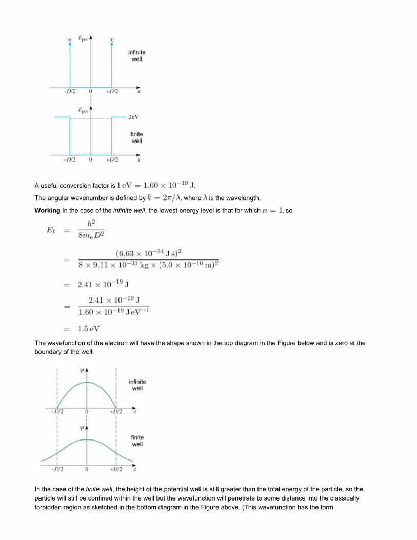
Working In the case of the infinite well, the lowest energy level is that for which , so

The wavefunction of the electron will have the shape shown in the top diagram in the Figure below and is zero at the

boundary of the well.

In the case of the finite well, the height of the potential well is still greater than the total energy of the particle, so the

particle will still be confined within the well but the wavefunction will penetrate to some distance into the classically

forbidden region as sketched in the bottom diagram in the Figure above. (This wavefunction has the form

in the region inside the well.)

The wavefunction now clearly has a longer wavelength, since it has to match an exponentially decaying value at the

boundary. Hence, since it has a smaller value of the angular wavenumber than does the wavefunction in the

case of the infinite well. The value of is related to the energy according to so a smaller value of

corresponds to a smaller value of .

Thus the energy of the particle in its lowest energy state is smaller when it is confined in the finite well than when it is

confined in the infinite well.

Checking Is this result physically reasonable? According to Heisenberg’s uncertainty principle, it is. In an infinite well

(especially a very narrow one), we are fairly certain of the particle’s position because it is completely trapped with no

possibility of being found outside the confines of the well. Hence the uncertainty in its position ( in one dimension) is

small. The corresponding uncertainty in its momentum is therefore high. If there is a large spread of possible

momenta for the particle, on average its momentum must be high and its average kinetic energy must also be high. So

the lowest energy state of the particle is of greater energy the deeper (and narrower) the well. We can also check that the

energy has the correct units, as indeed it does (joule and electronvolt) and that its value is reasonable. Finally, it is useful

to check that when sketching the wavefunctions we have labelled the axes, indicated the important values ( and

) and labelled them clearly.

Example 2

A particle of mass and total energy has the potential energy function shown in

the Figure below; this consists of a square potential energy barrier of height and width

. Schrödinger’s equation for this particle takes the form

where is a suitable potential energy function. In the region from to , the wavefunction describing

the particle can be written in the form

where and are constants.

(a) By differentiation, show that this wavefunction does satisfy Schrödinger’s equation in the region from to

. What is the value of the constant ?

(b) Suppose that the probability of finding the particle in a small region near is . What is the probability of

finding the particle in a similar region near ?

To view the solution, click on Video 1 below. Full-screen display is recommended.

DownloadVideo 1 Solution to Example 2.

3.7 A particle confined in three dimensions

When a particle is confined in one dimension between two walls, the solutions of Schrödinger’s equation in Section 3.1 and

Section 3.4 showed that the particle should have energy levels, characterised by a single integer (Equation 12). These

solutions were very similar to the solutions of the wave equation for the allowed standing waves on a stretched string that you

met in Unit 14. It is fairly easy to extend this example to two or three dimensions. Suppose we have a two-dimensional

surface, such as a drum consisting of a skin stretched over a square frame. In this case, it is reasonable to expect that the

kind of standing waves that can be set up must satisfy independently the condition that a whole number of half-wavelengths

can fit into each of the two coordinate directions, with nodes at the edges. This means that two independent integers are

needed to specify the various standing waves that can exist. Figure 13 shows some of the possible standing waves that can

be set up on such a surface.

Figure 13 Some standing wave patterns on a square,

two-dimensional surface. The numbers and indicate the

number of half-wavelengths in the - and -directions,

respectively.

This idea can be extended to three dimensions, in which case three independent integers now specify the allowed standing

waves. When we come to solve the Schrödinger equation for a particle confined in an infinite square well in two or three

dimensions, we find the equation must be solved for each direction separately, satisfying the condition that on all of

the boundaries. So, in the same way as we found for the one-dimensional case, we find that the allowed wavefunctions have

wavelengths of only certain, definite values. Thus a particle confined in a hollow cubical box will have only certain, definite

values of energy, i.e. energy levels. What are these values of energy?

You saw in Section 3.1 that the energy levels of a particle confined in one dimension are given by

The corresponding formula for the energy levels of a particle confined in three dimensions (in a hollow cubical box) has a

similar form:

The integers , and specify the number of half-wavelengths that are fitted into each of the three directions parallel to

the edges of the box.

An intriguing new effect now comes into play.

Exercise 7

Determine the energy that corresponds to the following sets of values:

(18)

(i) , ,

(ii) , ,

(iii) , and

Express your answer as the product of a number and the factor

Answer

Using Equation 18:

we have in each of the three cases

The exercise above shows that a particle confined in three dimensions can have the same total energy even if it is described

by different sets of integers , and . This phenomenon is known as degeneracy. When the same energy value arises

from different sets of integers , , , the different combinations are said to be degenerate in energy. Each different set

of quantum numbers , , , specifies a particular quantum state of the system. Thus a particular energy level will be

degenerate if it corresponds to more than one quantum state. It is important to be aware of this distinction between quantum

states and energy levels. The concept of degeneracy is very important, and although we shall not pursue it further at present,

you will see in Unit 21 that it plays a crucial role in interpreting the allowed energy levels of the electron in the hydrogen atom.

While discussing the three-dimensional case, it is useful to extend another idea that you have met already in Section 3.2. In

the one-dimensional example of the particle confined between two walls, the probability of finding the particle in a region of

width was given by Equation 15

assuming that the normalisation process has been carried out. This idea can be extended naturally to three dimensions, so

that the probability of finding a particle represented by a three-dimensional standing wave described by the time-independent

wavefunction in a small volume element is similarly given by

As in one dimension, it is necessary to normalise so that the total probability of detecting the particle somewhere in the

three-dimensional volume in which it is confined is equal to one.

3.8 Quantisation and the everyday world

In the previous subsections, you saw that the effect of confining a particle is to limit its allowed energy to certain discrete

values. Why, then, don’t we see evidence for such quantisation in the everyday world?

The classical and quantum-mechanical viewpoints can be reconciled by remembering that, for everyday objects, the energies

involved are huge in comparison with . This implies that the quantum numbers, , that specify these energies

are correspondingly huge. Therefore, the energy difference between consecutive states (states corresponding to and

) is too small to be observed, i.e., the energy is not observed to have discrete values.

When is very big, there is a very large number of half-wavelengths in the standing probability wave that describes a particle

confined in one dimension between two reflecting walls (Figure 14a). The probability of detecting the particle in a small region

(19)

between the walls at the scales discernable by human senses is then independent of the region’s location (Figure 14b).

Figure 14 When the behaviour of a confined particle

(Figure 4 shows a 1D particle in a box for illustration) is

described by a probability wave characterised by a high value

of as in (a), the probability of detecting the particle in a

region of given size is approximately independent of the

location of the region between the walls, as in (b). As tends

to infinity, the classical limit is approached, i.e. the probability

of detecting the particle in a region of a given size is

independent of the region’s location. This illustrates the

correspondence principle.

This agrees with expectations based on classical physics — if an experiment to find the position of the confined particle is

performed at random, it is found that the particle is equally likely to be detected at any position between the walls. The

conclusion is that when the number characterising the particle’s probability wave (and energy level) is very large, the

quantum-mechanical description of the particle becomes almost identical to its classical description.

Now look at Example 3, in order to examine some more predictions that quantum mechanics makes about macroscopic

objects.

Example 3

Calculate the minimum kinetic energy that a small glass bead of mass can have when it is confined

between two rigid walls that are apart. Assuming that we can interpret this energy as the kinetic energy of the

bead as it moves with a speed , calculate this speed and hence the time the bead would take to cross the box.

Answer

We can model the bead as a particle confined in an infinite square well. The allowed energies are then given by

Equation 12:

The minimum energy of the bead occurs when . With ,

Classically, if we interpret this energy as a kinetic energy, then the bead must have speed such that , so

to two significant figures. The time taken to cross the box at this speed is

i.e. about !

The speed you have calculated in your answer to Example 3 is infinitesimally small, and this means that a macroscopic

object, such as a glass bead, is effectively at rest when it occupies its lowest energy level.

Example 4

Suppose that the glass bead in Example 3 is travelling at a speed such that it travels between the walls in . What is

its total energy? Assuming it to be in a stationary state with this energy, to what value of does this energy correspond?

Comment on your result. (Assume that between the walls.)

Answer

The bead has a mass of and speed ( ), so its kinetic energy is given by

. The allowed energy levels of the bead are given by Equation 12.

Equating this quantity with the total energy of the glass bead gives

and therefore

so .

This extremely large value for implies that the standing wave representing the bead has a correspondingly large

number of nodes between the walls of the box. In this case, the distance between nodes of the wave is too short to be

measurable and therefore the probability of finding the bead will be detected as the same throughout the box.

Example 3 and Example 4 demonstrate that quantum effects cannot be detected for macroscopic objects. In the next section

you will see how the effects of quantum physics may be reconciled with the predictions of classical physics.

3.9 The correspondence principle

Your answers to Example 3 and Example 4 should have convinced you that the discrete effects predicted by quantum

mechanics (e.g. the energy levels of a confined particle) are unobservable when they are applied to everyday problems —

quantum effects can safely be neglected in such situations. To put it more broadly, the predictions of quantum mechanics

become practically identical with those of classical mechanics when they are applied to problems about the macroscopic

world. This is analogous to the way in which the predictions of special relativity become practically identical to the

corresponding predictions of non-relativistic mechanics at speeds much less than the speed of light (Section 6.4 of Unit 13).

Quantum mechanics is believed to provide a more general and correct description of matter than classical mechanics, but it

is nevertheless true that quantum mechanics contains the more familiar ideas of Newtonian (classical) mechanics within its

framework. In Example 3 and Example 4, you have encountered a one-dimensional example (the motion of a glass bead

between the reflecting walls) in which the quantum-mechanical description of the system is indistinguishable from the

corresponding classical predictions. The idea that quantum mechanics must have a classical limit is embodied in the

so-called correspondence principle. In fact, as shown in Example 4, the classical limit is equivalent to the limit in which the

number in Equation 12 becomes very large.

The correspondence principle

In the limit of large quantum numbers, known as the classical limit, the predictions of quantum mechanics are in

agreement with those of classical mechanics.

This is a profoundly important principle. It says, in effect, that in the limit of large quantum numbers, the predictions of

quantum mechanics must be indistinguishable from those of classical (Newtonian) mechanics. We should expect this to be

the case since classical mechanics is an extremely successful theory when applied to matter on the large scale.

Exercise 8

In a crude model of the hydrogen atom, it is assumed that the electron in the atom is confined in a hollow, cubical box

whose sides each have a length of .

(a) Using Equation 18, write down a formula that gives the energy levels of the electron in the hydrogen atom according

to this model.

Answer

where and , and can each take values

(b) What is the spacing of the two lowest energy levels of the electron according to this model? How well does this

prediction of the model compare with the experimentally measured spacing of ?

Answer

The lowest energy level is characterised by , and so .

The second lowest energy level is characterised by or or

: these three states are degenerate since they each describe the electron when it has total

energy of .

According to this model, the spacing of these two energy levels is

i.e.

This prediction agrees very well with the experimentally measured value of the spacing .

(c) Give at least one reason why this model of the hydrogen atom is inadequate.

Answer

The model does not take account of the fact that the electrostatic attractive force on the electron, , varies with its

distance from the centre of the nucleus.

Comment: A more careful investigation of the model shows that its prediction for the spacings of the electron’s higher

energy levels is in gross disagreement with experiment.

Exercise 9

A particle of mass is confined by infinitely high walls so that it moves in two dimensions within a square whose sides

have length . By referring to the form of the equations for the allowed energy levels of standing waves in one dimension

and three dimensions (Equation 12 and Equation 18), write down the expression for the energy levels of this confined

particle. How many degenerate states are there for each of the three lowest energy levels?

Answer

The energy levels of the particle are given by

where is the length of each side of the square. The particle’s three lowest energy levels are characterised by:

(i) : there is no degeneracy here.

(ii) and : these two states are degenerate since they both describe the particle

when it has a total energy of .

(iii) ( , ): there is no degeneracy here.

4 Description, prediction and measurement in quantum mechanics

This section is mainly concerned with the way in which quantum mechanics is used to describe the state of a physical

system, and to predict measurable properties associated with that state. That is to say, it is concerned mainly with formalism.

After a brief review of the formalism introduced in this Unit, it extends the formalism by introducing the related concepts of

eigenstate and eigenvalue, and by explaining the importance of linear superposition and coherence in quantum mechanics.

The example of two-slit electron diffraction introduced in Section 4.3 of Unit 19 will be used throughout to highlight these

ideas.

4.1 Quantum systems

The starting point of any application of quantum mechanics is the identification and specification of the system to which the

formalism will be applied. Such a system is often referred to as a quantum system, though its specification generally

involves purely classical concepts. You have already met many examples of one-dimensional quantum systems in which the

potential energy of the particle was described by a function that was either a well or a barrier. Examples of atoms

as more complicated quantum systems will be introduced in the next Unit.

Another example of a quantum system is provided by the idealised two-slit electron diffraction apparatus shown in Figure 15.

In this case, electrons (i.e. particles of mass and charge travelling from the electron gun to the fluorescent screen

encounter a diaphragm that is impenetrable apart from two narrow slits, each of width , the centres of which are

separated by a distance . Although this system was introduced earlier, it was not treated in detail. Had it been subjected to

a detailed analysis, we would have found it useful to introduce a coordinate system of the kind shown in Figure 15, and we

would have described the influence of the diaphragm using some potential energy function that would have

involved the parameters and amongst others. This would have been a crucial part of our specification of the system.

Figure 15 A two-slit electron diffraction apparatus. Here, the

screen shows the kind of interference pattern that would be

observed when an intense steady beam of electrons flows

through the apparatus. The bright bands correspond to places

where large numbers of electrons arrive, and the dark bands

are places where few, if any, arrive. (Note that the slit width

and separation are greatly exaggerated.)

The main point to take away from this discussion is the following:

The specification of a quantum system typically involves a number of parameters (such as and and a potential

energy function .

4.2 States and observables

Having specified a system of interest, the next step in applying the formalism of quantum mechanics is to investigate the

possible states of that system. The state of a system refers to the condition of the system, and implies a sufficiently detailed

description of that condition to distinguish it from any other condition that would cause the system to exhibit different

behaviour.

Both classical mechanics and quantum mechanics make use of the concept of state, and both kinds of mechanics relate the

concept of a state to measurable properties such as position, energy and momentum. These measurable properties of a

physical system are referred to as the observables of the system, and it is the values of a system’s observables that are

generally the focus of experimental interest. However, where classical mechanics and quantum mechanics differ is in the way

they describe the state of a system, and in the way they relate the state to the values of the system’s observables. These

differences are profound and important, so we shall discuss them in some detail.

In classical mechanics, specifying the state of a system involves assigning values to sufficient of its observables to uniquely

determine the state. For instance, to specify the state of a particular golf ball, you might give the simultaneous values of its

position, its velocity, its acceleration and its angular momentum. These values would determine the condition of the golf ball

at some particular time, and could be used as the starting point for an equally detailed prediction of its condition at some

future time.

Contrast this with the situation in quantum mechanics. There, specifying the state of a system generally implies specifying the

time-dependent wavefunction that corresponds to the state. The wavefunction is found by solving an appropriately

formulated version of the time-dependent Schrödinger equation — one that takes full account of any system-specific

parameters such as masses and charges, as well as the relevant potential energy function. Not until the Schrödinger

equation has been solved and the appropriate wavefunction determined is it possible to make detailed statements regarding

the values of observables such as position or momentum. Even then, the sort of statements that quantum mechanics permits

are quite different from those allowed in classical mechanics. In the quantum-mechanical case, Heisenberg’s uncertainty

principle will limit the extent to which the values of certain pairs of observables can be simultaneously determined, and for

any given observable the most that can generally be predicted in advance of a measurement are the possible outcomes of

that measurement and the probability of each of those possible outcomes.

Consider again the two-slit electron diffraction experiment illustrated in Figure 15, but suppose now that the intensity of the

electron beam is reduced to such an extent that electrons pass through the diffraction apparatus one at a time. The arrival of

a single electron at the screen will create a single spot of light on the screen, thus revealing the particle-like nature of the

electron (Figure 16a). However, if, over a period of time, the spots created by the arrival of a large number of individual

electrons are recorded, then it will be found that they form an interference pattern similar to that created by a steady intense

beam (see Figure 16b). This is a clear indication of the wave-like nature of the electron. It is the task of quantum mechanics

to provide a coherent account of the behaviour of a system that exhibits this classically contradictory wave–particle duality.

This is what Schrödinger’s wave mechanics achieves, by using a wavefunction to describe the state of the system.

Figure 16 (a) In a two-slit electron diffraction experiment, the

arrival of a single electron at the screen creates a single spot of

illumination. (b) A record of the spots created by many such

individual electrons will reproduce the interference pattern

produced by an intense beam of electrons.

The state of an electron that sets out from the electron gun, at , at some time close to , and travels towards the

screen, can be described by a wavefunction that takes the form of a (complex) travelling wave packet. At time

, when the electron is just starting out on its journey to the screen, its wavefunction will be concentrated near the

electron gun. As increases, the wave packet will evolve, moving towards the screen and spreading out as it does so, as

indicated in Figure 17.

Figure 17 The changing wavefunction of a single electron in a

two-slit diffraction experiment. The wavefunction itself is a complex

quantity, so it cannot be easily illustrated; for this reason the

diagram actually shows the value of the (real) positive quantity

at various times, and it displays these values as contour

plots. Even so, the figure is highly schematic and makes no

attempt to accurately represent the detailed wavefunctions that

can be computed for this situation.

(The increasing spread of the wavefunction is a consequence of the unavoidable uncertainty in the initial momentum of the

localised electron.) The encounter with the slits will divide the wave packet into two parts, but they are both parts of the same

wave packet and still describe the state of a single electron. As time continues to pass, the two parts of the evolving

wavefunction will overlap and interfere. At time , when the electron might be observed to arrive at the screen, the

value of the wavefunction at a point on the screen with coordinates will be given by . The range of

and values for which is not zero determines the possible outcomes of a measurement of the electron’s

arrival point on the screen, while the function determines the relative probability of each of those possible

outcomes. The fact that this latter function has the form of a two-slit interference pattern ensures that the detection of many

individual electrons, each described by a similar wavefunction, will eventually create the observed interference pattern.

4.3 Eigenstates and eigenvalues

Of course, it is always possible that the state of a quantum system will be such that a measurement of some selected

observable has only one possible outcome. In other words that there is a possible outcome that is predicted to occur with

probability When this is the case, the state of the system is said to be an eigenstate of the selected observable, and the

one value that will inevitably be obtained for the observable when the measurement is made is said to be the eigenvalue of

the observable that corresponds to that particular eigenstate (the word ‘eigen’ comes from the German for ‘characteristic’).

Many of the wavefunctions that were discussed earlier in the Unit represented eigenstates of energy, since many of them

corresponded to a single value of the energy observable. Such functions are found by solving the time-independent

Schrödinger equation (Equation 4) . Each of the time-independent wavefunctions that satisfies this equation corresponds to

some particular value of the total energy , which represents the eigenvalue of energy associated with that solution.

As an example, consider the energy eigenstates for a particle of mass confined in an infinite square well of width .

These particular eigenstates correspond to different values of a quantum number, , that has been used to label the different

time-independent wavefunctions, which have the form and with .

As you saw earlier in the Unit, this quantum number also appears in the expression for the corresponding energy

eigenvalues, (Equation 12), so to make this explicit we can write:

Exercise 10

What is the eigenvalue of energy, in electronvolts, associated with the state of an electron in an infinite square potential

well with for each value of given below?

(a) 

Answer

The energy levels are given by

Thus:

(b) 

Answer

Using the same expression .

The fact that the energy eigenstates of confined systems are also stationary states gives them a special significance and

makes them especially easy to discuss. However, it is important to note that the concepts of eigenstate and eigenvalue are

quite general and may be applied to any observable, not just to energy.

Eigenstates and eigenvalues play an important part in quantum mechanics. Historically, the series of scientific papers in

which Schrödinger introduced his formulation of quantum mechanics (published in the German journal Annalen der Physik, in

1926) were collectively entitled ‘Quantisation as an Eigenvalue Problem’. The fact of the matter is that, according to quantum

mechanics, the result yielded by a measurement of any observable must be an eigenvalue corresponding to some particular

eigenstate of that observable. This is true, whatever the state of the system prior to the measurement. If we know the state

prior to the measurement, then quantum mechanics enables us to predict which of the various eigenvalues is a possible

result. It also allows us to calculate the probability of each of those possible results. But even if we don’t know the state of the

system, we can still be sure that when we measure some observable, the result will be an eigenvalue corresponding to some

eigenstate of that observable.

Exercise 11

A measurement is performed on a particle in an infinite square well. The energy of the particle is measured to correspond

to . What state was the particle in, immediately prior to the measurement?

Answer

We cannot say. All we can say is that the wavefunction that described it before measurement would have had a

contribution from the energy eigenstate given by . But this does not mean that the particle was in this state.

We shall have more to say about the significance of this later. For the moment, here is a reminder of the key points.

The eigenvalues of a given observable are the only possible outcomes of any measurement of that observable.

The state of the system (as described by its wavefunction) determines the relative probability of measuring each of

those eigenvalues.

A state in which a particular eigenvalue is predicted with probability is said to be an eigenstate of the given observable

and may be said to correspond to the relevant eigenvalue.

4.4 Superposition states

Many of the peculiarities of quantum mechanics can be traced to one fundamental feature of the mathematical formalism: the

fact that any two solutions of a system’s time-dependent Schrödinger equation can be combined to produce a third solution.

We can use the wavefunctions of the particle in the infinite square well to illustrate this important fact.

Suppose that and are the normalised time-dependent wavefunctions that correspond to the

time-independent wavefunctions and in an infinite square well . Since and are both

solutions to the time-dependent Schrödinger equation for a particle in an infinite square well, it follows from the mathematical

nature of the Schrödinger equation that their sum

will also be a solution and will therefore represent a possible wavefunction of the system. This sum would not represent a

normalised wavefunction, but we can easily scale it to produce the normalised wavefunction

Such a wavefunction is said to be a normalised linear superposition of the wavefunctions and , and the state

described by that linear superposition may be referred to as a superposition state.

The reason why a superposition state of this kind is interesting, and so very characteristic of quantum mechanics, is that it

combines features that would appear self-contradictory in a classical state. In the case of Equation 20, for example, the

wavefunction consists of equal contributions from eigenfunctions corresponding to two different energy eigenvalues;

and . This means that if things are arranged in such a way that the particle in the

infinite well is actually in the state described by Equation 20, then a measurement of the energy of that particle has two

possible outcomes or , and the probability of obtaining either result is . This implies that in, say, one thousand

measurements of energy, performed on the same system, prepared each time in the same superposed state, the result will

be on about occasions, and on about occasions. The fact that identical measurements repeatedly carried

out on an identically prepared system can lead to different outcomes is typical of quantum mechanics, but it is totally at odds

with classical mechanics.

The process of forming linear superpositions is not restricted to eigenfunctions of energy, nor is it restricted to equal

combinations of two solutions of Schrödinger’s equation. Any solutions of the relevant time-dependent Schrödinger equation

may be linearly superposed, and we can combine as many of those solutions as we wish. The general rule for forming such

combinations is known as the principle of superposition, and may be expressed as follows.

The principle of superposition

If , , , are solutions of the time-dependent Schrödinger equation for a given system, then that

equation will also be satisfied by any linear superposition of the form

where , , are numbers that are, in general, complex.

A ‘visualisation’ of the process of linear superposition is shown in Figure 18. As you can see, the process is similar to that of

adding component vectors to produce a resultant vector, though in the case of linear superpositions there may well be more

than three independent ‘directions’ and the coefficients may be complex. We shall not pursue the analogy

between linear superposition and vector addition here, but the relationship is a deep one.

Figure 18 A visualisation of the process of linear superposition.

This figure is not supposed to represent any particular linear

superposition, but rather to suggest an analogy between the linear

superposition of wavefunctions (with complex coefficients) and the

summation of vectors (with real coefficients).

(20)

(21)

a. and

b. and

c. and

d. and

Exercise 12

What are the values of and in the linear superposition below?

The correct answer is c.

Answer

We can rewrite

therefore and .

4.4.1 Normalisation and linear superposition

The general linear superposition described by Equation 21 is not necessarily normalised. However, it will be normalised if two

additional conditions are also satisfied:

The wavefunctions , , are individually normalised.1.

The numbers are such that2.

Provided both these conditions are satisfied, will be a normalised wavefunction, and the particle it describes will therefore

have a probability of of being found somewhere when its position is measured.

Exercise 13

If and are individually normalised, is the linear superposition also normalised?

Answer

Yes, because and , so .

The great advantage of dealing with normalised linear superpositions is that they lead to simple predictions concerning the

probabilities of predicted measurement outcomes. This point is most easily made by considering an example. Suppose ,

and are three eigenstates of energy for some quantum system, corresponding to the energy eigenvalues , and

. If the state of the system is represented by the linear superposition

then the only possible outcomes of a measurement of the energy will be or or . Quantum mechanics does not

allow us to say which of the three possible values will result from any particular measurement performed on the system while

it is in the state described by Equation 23, but, provided the linear superposition has been normalised, quantum mechanics

(22)

(23)

does predict the probability of each of the possible outcomes. If we denote the three probabilities by , and

, quantum mechanics predicts that:

Note that, because we are dealing with a normalised superposition, it is certain to be the case that

. This implies that, as long as the system remains in the superposed state, the probability that

a measurement of the system’s energy will result in one of the three possible outcomes is i.e. it is certain.

This simple relationship between linear superpositions and predicted probabilities can be generalised to any linear

superposition of eigenstates for any observable. In general, if we consider some observable (not necessarily the energy)

with eigenvalues , , , then we can say the following.

Given a system in a state represented by the normalised wavefunction

where the normalised wavefunctions represent eigenstates of some observable , and

correspond, respectively, to eigenvalues then the only possible outcome of any measurement of that

observable is one of those eigenvalues, and the probability that it will be is given by

It’s worth stressing again that the wavefunctions referred to here, which represent eigenstates of the observable , are

not necessarily eigenstates of energy. The general indeterminacy of quantum mechanics that prevents particles from

simultaneously having precisely determined positions and momenta, may actually prevent the eigenstates of the observable

from also being eigenstates of energy.

Exercise 14

A quantum system has been prepared in such a way that its state is described by the wavefunction

, where the normalised wavefunction represents an eigenstate of energy, with

corresponding to the eigenvalue , for . Confirm that is a normalised wavefunction, and write

down the probabilities that the energy of the system will be measured to be that corresponding to , and

.

Answer

The fact that the given state is normalised is guaranteed by (i) the fact that each of the eigenstates is normalised, and

(ii) the sum of the squared moduli of all of the coefficients in the linear superposition is equal to

In this case those coefficients are , , , ; and

The probability of each eigenvalue is given by the square of the modulus of the coefficient of the corresponding

eigenstate. There is no eigenstate corresponding to , so that is not a possible result and therefore has zero

probability ( ). For the other results, the probabilities are

(24)

4.4.2 Superpositions and two-slit electron diffraction

It is instructive to apply the idea of a superposition state to the two-slit electron diffraction experiment we discussed earlier.

Figure 19 shows a modification of the original arrangement in which the slits are labelled and and one of the slits is

blocked.

View larger imageFigure 19 (a) A two-slit electron diffraction

apparatus in which slit has been blocked. The screen shows a

single-slit diffraction pattern rather than a two-slit interference

pattern. (b) Opening slit and closing slit changes the

wavefunction of electrons passing through the system, but

hardly affects the pattern recorded on the screen.

If slit is blocked, each electron must travel through slit , and the state of each of those electrons can be described by a

wavefunction that reflects this. Recording the arrival of a large number of those electrons on the screen will produce the

single-slit diffraction pattern shown in Figure 19, not the two-slit interference pattern we have already seen, and that is

repeated in Figure 20. If slit is opened and slit closed, the state of each electron will be described by a somewhat different

wavefunction, , but the pattern recorded on the screen will be practically unchanged — it will again be a single-slit

diffraction pattern. However, if both slits are open, the state of each electron can be represented by the linear superposition

and the pattern recorded on the screen will be the two-slit interference pattern of Figure 20.

Figure 20 The two-slit interference pattern recorded when both

slits are open.

When only one slit is open, the intensity pattern will be proportional to either or , but when both slits are open

the intensity is proportional to

It is this latter intensity distribution that accounts for the interference effects seen when both slits are open. As a result, when

both slits are open there will be points on the fluorescent screen where electrons will never be observed, even though

electrons may be seen at those points when either slit or slit is open on its own.

The important point to note about this is that the function represented by is quite different from the function

represented by or or even . To say that the wavefunction of a system is

is not the same as saying that the wavefunction is either or , even with probabilities attached to

the two alternatives. The wavefunctions and individually correspond to classically comprehensible statements about

the electron — ‘it went through slit ’ or ‘it went through slit ’ — but the linear superposition does not. In

particular, it does not correspond to the statement ‘either the particle went through slit or it went through slit ’. Rather, it

corresponds to the non-classical statement that ‘the particle was free to go through both of the slits in an indeterminate way’.

(25)

As long as the route of each electron is indeterminate the contributions represented by and are said to add in a

coherent manner, implying that they can interfere (like coherent beams of light) and it is then that their joint effect results in

an intensity distribution that is proportional to . Modifying the experiment so that it becomes possible to say

which slit each electron went through would remove the indeterminacy and destroy the coherence. As a result, the intensity

distribution would be proportional to an ‘incoherent’ sum of the form , and the interference effects would

vanish. This will be true irrespective of how the path of the electron was determined.

4.5 Measurement in quantum mechanics

4.5.1 Measurement, indeterminacy and indeterminism

Observing a spot on a fluorescent screen at , constitutes a measurement of the electron’s position (specifically, of its

- and -coordinates). The process of measurement provides information about the values of observables at a particular

time. Indeed, in quantum mechanics, statements about the value of an observable only become meaningful in the context of

a measurement. In the absence of an actual measurement, the most we can say about the value of an observable is what we

can learn from the wavefunction that describes the state of the system, and that, as we have already stressed, is limited to

the possible outcomes of a measurement and the probability of each of those possible outcomes. Therefore, it is clear that

measurement plays a crucial role in quantum mechanics by turning a potentiality (a possible outcome with an associated

probability) into an actuality (a measured result).

Nobody who has studied classical physics would have much difficulty in understanding a statement such as, ‘An electron

moving with constant velocity , and which passes through the origin at time , will reach the point

at time .’ However, this is just the kind of statement that quantum mechanics does not allow us to

make about an electron. There are two general features of quantum mechanics that limit what can be said about

measurements of observables.

Indeterminacy. The impossibility of measuring, with total precision, the values of all the observables of a quantum

system simultaneously is known as indeterminacy. It is always possible to find pairs of observables that cannot be

precisely measured at the same time. Heisenberg’s uncertainty principle for position and momentum provides the

best known example of this, but indeterminacy is a general feature of quantum mechanics, the uncertainty principle

for position and momentum simply brought it to light.

1.

Indeterminism. The fact that, in quantum mechanics, determining the precise values of some observables at a

particular time will not generally determine the precise values of those observables at later times is known as

indeterminism. This is in sharp contrast to classical mechanics, which is fully deterministic, implying that

measurements of certain observables at one time do determine the values of those observables at later times.

2.

It is important to realise that the indeterminacy and indeterminism of quantum mechanics are both matters of principle. They

are consequences of the mathematical structure of the formalism and have nothing to do with practical considerations about

the difficulty of taking accurate experimental readings or anything of that nature.

When thinking about the states and observables of a quantum system it is always useful to keep indeterminacy and

indeterminism in mind. This will help you to avoid using concepts that cannot be justified. In the case of two-slit electron

diffraction, for example, it is tempting to suppose that the electron follows a definite but unknown path through the apparatus,

and that the use of wavefunctions simply provides a way of dealing with our ignorance of the details of the motion. This,

however, is not the case. According to the conventional interpretation of quantum mechanics, the electron’s position only has

a value when it is measured. In the absence of a measurement, the electron’s position is not just unknown, but indeterminate.

Prior to the measurement, the electron is not at some unknown position, rather, it is not at any position at all.

Exercise 15

Consider a double slit experiment and imagine that a measuring device is placed between the slits and the screen to

determine the position of the electron at a certain time before it reaches the screen. Will this allow us to predict the point

at which the electron will reach the screen?

Answer

The measuring device allows us to determine the position of the electron, thus making it determinate. Nonetheless, this

knowledge won’t allow us to predict where the electron will hit the screen. The indeterminism of quantum mechanics

prevents that.

In the absence of a measurement, the formalism of quantum mechanics neither provides nor requires any information about

the precise position of the electron at any time. The coordinates and that appear in the argument of the wavefunction

simply label points where the electron might be found if a measurement is performed — they are not the

instantaneous position coordinates of the electron at time . By analysing the wavefunction it is possible to determine all the

possible outcomes of a measurement of position (or, in fact, of any other observable) at time , and to predict the probability

of each of those possible outcomes. However, the formalism of quantum mechanics does not give any general procedure for

predicting the precise outcome of any particular measurement. The prediction of possible outcomes and their respective

probabilities is as far as quantum mechanics goes. This point was made at the start of our discussion of quantum mechanics,

but it is of such importance that it deserves to be highlighted again.

4.5.2 The nature and effect of a measurement

Although the term ‘measurement’ has already been used several times it has not so far been properly defined. In quantum

mechanics, measurement is a technical term with a precise meaning. It describes a physical interaction between a quantum

system and a measuring device that results in the measuring device being left in some state that represents the outcome of

the measurement. The final state of the measuring device might, for example, correspond to a reading on a scale, or an

orientation of a pointer, or just some combination of indicator lights being on rather than off.

Now, a measurement performed on a quantum system has no point unless it provides information about the state of that

system. What, then, does a measurement of a certain observable , that yields the result , tell us about the state of the

measured system? The conventional answer to this question is this:

Immediately after a measurement of an observable , the state of the measured system will be the eigenstate of that

corresponds to the measured eigenvalue .

So, according to this conventional view, the process of making a measurement will force the system into the eigenstate that

corresponds to the measured result. This eigenstate may not have been the state before the measurement, but it will be the

state immediately after the measurement. This can be confirmed by making another measurement of the same observable,

, immediately after the first. If the second measurement really is performed immediately after the first, its outcome is certain

to be the same as the first. But the only state that guarantees a definite outcome of this kind is one that is an eigenstate of

the measured observable.

Now consider the implications of this for a system that, prior to a measurement of observable , is in a state described by

the linear superposition

where , , are normalised wavefunctions that represent eigenstates of the observable , corresponding

to eigenvalues , , If is measured, and the result is obtained, then immediately after that

measurement the state of the system will be represented by the wavefunction This abrupt change in the system’s

wavefunction, from to is described by saying that the measurement causes the collapse of the wavefunction.

The collapse of a wavefunction can be illustrated by looking again at the case of single electrons passing through the two-slit

diffraction apparatus of Figure 16. As discussed in Section 4.4.2, if no steps are taken to determine which slit an individual

electron passes through, the intensity distribution created by a large number of electrons arriving at the screen will be

described by , i.e. the familiar two-slit interference pattern of Figure 20. (Remember that here and

are time-dependent wavefunctions corresponding respectively to passage through slit or slit )

The result of observing the arrival at the screen of a large number of electrons that have had their wavefunctions collapsed

by an earlier measurement that reveals which slit it passed through will be described by an incoherent sum of the form

— the sum of two single-slit diffraction patterns, of the kind shown in Figure 19.

The process of wavefunction collapse is illustrated in a highly schematic way in Figure 21.

Figure 21 A highly schematic view of the process of wavefunction

collapse. Prior to the collapse the wavefunction consists of two

parts that describe different eigenstates of a given observable.

These are indicated by perpendicular vectors, corresponding to

and . After the measurement, the wavefunction has collapsed

onto one of those two eigenstates. Overall normalisation is

preserved throughout.

It was said earlier that quantum mechanics predicts the possible outcomes of a measurement and the probability of each of

those possible outcomes. You should now be able to see that an alternative way of expressing this is to say that quantum

mechanics predicts the possible states to which the wavefunction of a system might collapse, and the probability that it will

collapse to each of those possible states. However, just as quantum mechanics does not generally predict the precise result

of a particular measurement, so it does not predict the precise eigenstate to which the wavefunction will collapse as a result

of a particular measurement. To that extent the collapse of the wavefunction is unpredictable as well as abrupt.

Exercise 16

A quantum system is initially in a state described by the wavefunction where and are

normalised wavefunctions describing eigenstates of energy that correspond to eigenvalues and , respectively. If a

measurement shows that the energy of the system is , what is the wavefunction of the atom immediately after the

measurement?

Answer

Immediately after the measurement the wavefunction of the system will be .

5 Interpretation

The audios in the following subsections provide an interesting background on the various interpretations of quantum

mechanics.

5.1 The Copenhagen interpretation

The Copenhagen interpretation puts particular emphasis on measurement since it assumes that measuring devices are

essentially classical pieces of apparatus (certainly, the readings they provide are ‘classical’). So measurement provides the

interface between a comprehensible world of classical objects and results, and a much less comprehensible world of

quantum systems and states that can be known only through the measurement results that it provides.

Figure 22 According to the Copenhagen interpretation,

measurements carried out on quantum systems must be

performed by devices that are essentially classical. The

interpretation therefore implies a ‘boundary’ that separates the

classical world of everyday objects from the quantum world that

underpins it.

Show transcriptDownloadAudio 3 Overview of the

Copenhagen interpretation.

5.2 Schrödinger’s cat and Wigner’s friend

Amongst the many physicists to experience disquiet over the interpretation of quantum mechanics, one of the most

prominent must surely have been Schrödinger himself. In 1935, while living in Oxford, in exile from the rising tide of Nazism

in his native Austria, Schrödinger published an article that highlighted some of his concerns. In the article he cleverly

emphasised the problem of making sense of measurement in quantum mechanics with his famous story of a cat in a box.

This poor beast is now known as Schrödinger’s cat.

Figure 23 Schrödinger’s cat, shut in a box with a radioactive

nucleus and a lethal contraption that will be triggered if and when

the nucleus decays.

Show transcriptDownloadAudio 4 Overview of

Schrödinger’s cat.

The decoherence effect is important in a number of applications. For example, avoiding them is key to building a working

quantum computer.

5.3 The many worlds interpretation

We briefly examine the famous (some would say infamous) many worlds interpretation of quantum mechanics. This

interpretation manages to avoid the conventional picture of a wavefunction that collapses at the moment of measurement.

The measuring devices that it involves can be treated as instruments that obey the rules of quantum physics, rather than

having to maintain the Copenhagen pretence that they are (logically at least) classical devices. The interpretation also offers

ways of avoiding the difficulties that arise when trying to make sense of superpositions of macroscopically different states, of

the kind highlighted by Schrödinger’s cat.

Since the 1980s, one of the most vocal supporters of the many worlds interpretation has been the British physicist David

Deutsch, a major contributor to the field of quantum computation. You can find out more about Deutsch’s own version of the

many worlds interpretation and its possible relevance to quantum computers in his popular book The Fabric of Reality,

(Penguin Books, 1997).

Figure 24 The branching, but not collapsing, wavefunction of the

many worlds interpretation.

Show transcriptDownloadAudio 5 Overview of the

many worlds interpretation.

5.4 Hidden variable theories and the ontological interpretation

The suggestion that quantum mechanics offers only an incomplete description of nature is an old one. Those who take this

view have often suggested that the behaviour of electrons and other microscopic entities is actually fully deterministic (rather

than inherently probabilistic as quantum mechanics asserts) and that a complete description of such entities involves certain

hidden variables that we have not yet learned to determine. Bohm’s theory, also known as the ontological interpretation,

is based on such hidden variables. A detailed account of this interpretation may be found in The Undivided Universe by D.

Bohm and B. J. Hiley (Routledge, 1995).

Figure 25 The (classical) trajectories of electrons passing

through the slits of a two-slit diffraction experiment according to

Bohm’s ontological interpretation of quantum mechanics.

Show transcriptDownloadAudio 6 Overview of hidden

variable theories.

6 Closing items

6.1 Achievements

After studying this Unit, you should be able to:

Explain the meaning of all the newly defined (emboldened) terms introduced in this Unit.

Discuss briefly what are meant by free (or unbound) and bound (or confined) particles, and describe qualitatively the

difference between the wavefunctions of particles in these conditions.

Describe how the Schrödinger equation is used to study the behaviour of particles. Sketch the time-independent

wavefunctions that are solutions to Schrödinger’s time-independent equation for some simple cases.

Relate the probability of detecting a particle in a region to the value of its wavefunction in the region, e.g.

.

Apply the formulae for the energy levels of a particle confined in one dimension between two infinitely high reflecting

walls and confined in three dimensions in a hollow cubical box.

Understand the implications of the correspondence principle and confirm it for simple cases.

Summarise the essential features of quantum mechanics in terms of systems, states, observables, predicted

measurement outcomes, indeterminacy and indeterminism.

State the superposition principle, and, in the case of a wavefunction that is a superposition of normalised wavefunctions

describing different eigenstates of some observable, relate the coefficients involved in that superposition to the

probabilities that measurements of the related observable will yield the various eigenvalues of that observable.

Outline the effect of a measurement on the wavefunction describing the state of a system, and discuss some of the

issues surrounding the process of wavefunction collapse.

Describe in qualitative terms the key features of various interpretations of quantum mechanics; specifically the

Copenhagen, many worlds and ontological interpretations.

6.2 End-of-Unit exercises

Exercise 17

A particle of mass is confined in one dimension between two infinitely high, rigid walls that are

separated by . The total energy of the particle is .

(a) What is the quantum number that characterises the wavefunction of the particle when it occupies this energy level?

Answer

The total energy levels of the confined particle are given by Equation 12:

Rearranging:

Using the information given in the question,

So the value of the quantum number that characterises the particle’s wavefunction (which must be an integer) is .

(b) Sketch a graph that shows the relative probabilities of detecting the particle in different regions between the walls.

Answer

For , the wavefunction has maxima and minima, as shown in the sketch below. The relative probabilities of

detecting the particle in different regions will be proportional to ; this is sketched in panel b of the same figure.

Exercise 18

A particle is confined in a one-dimensional finite square well such as that shown in the figure below. The depth of the well

is and the total energy of the particle is . Show that is a solution to the time-independent

Schrödinger equation for the particle in the region .

Answer

For , , so the time-independent Schrödinger equation appropriate to this region is

We have . Differentiating this twice gives

Substituting into the Schrödinger equation

Factors of can be cancelled such that

So is a solution to the Schrödinger equation provided

(here is a positive number since ).

Exercise 19

Criticise and suggest an improved rephrasing of the following statement about quantum mechanics. ‘Schrödinger’s

approach to quantum mechanics is all about systems with quantised energy, i.e. systems in which the energy can only

have certain discrete values.’

Answer

As it stands the statement is wrong. Quantum mechanics does describe such systems, but there is far more to quantum

mechanics than a discussion of quantised energy. A better formulation of the statement might be something along the

following lines:

‘Schrödinger’s approach to quantum mechanics is based on the use of wavefunctions that satisfy a differential equation

known as the time-dependent Schrödinger equation. This equation involves a potential energy function that allows the

equation to take on a form appropriate to specific problems. In the case of a particle confined within a potential well, the

Schrödinger equation implies that the measured energy of the particle will generally be quantised into discrete energy

levels. However, in other situations, such as that of a free particle, the measured value of energy may be any of a

continuous range of possible outcomes.’

Exercise 20

A particle of mass is confined in a hollow cubical three-dimensional box, each edge of which has a length , and for

which the potential energy function is zero inside, and infinite outside, the box. How many quantum states are there with

an energy of ?

Answer

The energy of the allowed states in a three-dimensional cubical box is given by Equation 18

Since we are given in this case , we see that . There are two different

sets of quantum numbers which will give this value, i.e. and The first set can be assigned in three different

ways:

The second set can be assigned in six different ways:

Hence there are quantum states that have this energy and the energy level is said to be nine-fold degenerate.

Exercise 21

Suppose that is the time-dependent wavefunction describing a system of two particles passing through the

double-slit diffraction apparatus that was described in Section 4. Given that the positions of the particles are indeterminate

prior to any measurement of them, what significance can be attached to any given set of values for the six position

coordinates and ?

Answer

The six coordinates ( and ( , should not be thought of as the position coordinates of the two

particles, since those positions are indeterminate. Rather, each combination of six values should be thought of as a

possible configuration of the system when it is measured. The time-dependent wavefunction can be used to determine the

probability that is to be associated with each of these possible configurations of the two particle system at time .

Exercise 22

The wavefunction describing the state of a certain quantum system is given by the linear superposition

, where and are normalised wavefunctions describing eigenstates of energy that correspond

to the eigenvalues and , respectively and is normalised.

(a) What is the value of the (real) constant ?

Answer

Given that and are both normalised, the normalisation of requires that .

Since is real, this implies that .

(b) What is the probability that a measurement of the atom’s energy will have the result ?

Answer

The probability of finding that the atom’s energy is is .

(c) What is the probability that the outcome will be ?

Answer

Since is not an eigenvalue that corresponds to either of the eigenstates in the superposition, the probability of

obtaining as the outcome of an energy measurement on the given state is zero.

6.3 Acknowledgements

Grateful acknowledgement is made to the following sources:

Figures

Figure 1: Bettmann / Corbis

Figure 6: Fritz Eschen / Ullstein Bild / Getty Images

Figure 25: Bohm, D. and Hiley, B. J. (1998) ‘The Undivided Universe: An Ontological Interpretation of Quantum Theory’,

Routledge, reproduced by permission of Taylor Francis Books UK

Every effort has been made to contact copyright holders. If any have been inadvertently overlooked the publishers will be

pleased to make the necessary arrangements at the first opportunity.