Unit 2 Introduction to Probability - UMasspeople.umass.edu/~biep540w/pdf/2. Introduction to...

PubHlth 540 – Fall 2010 2. Introduction to Probability of 57

Nature Sample

Observation/ Data

Relationships/ Modeling

Analysis/ Synthesis

Population/

Unit 2 Introduction to Probability

“Chance favours only those who know how to court her”

- Charles Nicolle

A weather report statement such as “the probability of rain today is 50%” is familiar and we have an intuition for what it means. But what does it really mean? Our intuitions about probability come from our experiences of relative frequencies of events. Counting! This unit is a very basic introduction to probability. It is limited to the “frequentist” approach. It’s important because we hope to generalize findings from data in a sample to the population from which the sample came. Valid inference from a sample to a population is best when the probability framework that links the sample to the population is known.


Nature Sample

Observation/ Data


Analysis/ Synthesis

Population/

Table of Contents

Topics

1. Unit Roadmap …………………………………………………………….. 2. Learning Objectives ………………………………………………………. 3. Why We Need Probability ………….……………..………………..……… 4. Definition Probability Model ……………..……………………………… 5. The “Equally Likely” Setting: Introduction to Probability Calculations ……..………………………….. 6. Some Useful Basics ……..…………………………..…..………………… a. Sample Space, Elementary Outcomes, Events ………………………… b. “Mutually Exclusive” and “Statistical Independence” Explained ……. c. Complement, Union, and Intersection ………………………………… 7. Independence, Dependence, and Conditional Probability ……………… 8. Some Useful Tools for Calculating Probabilities ………………………. a. The Addition Rule ……………………………………………………. b. The Multiplication Rule ……………………………………………… c Theorem of Total Probability …………………………………….…… d. Bayes Rule ……………………………………………………….…… 9. A Simple Probability Model: The Bernoulli Distribution ……………..… 10. Probability in Diagnostic Testing ………………………..……………… a. Prevalence…………………………………………………………...

b. Incidence ………………………………….……………..…..….…. c. Sensitivity, Specificity ………………………………………….… d. Predictive Value Positive, Negative Test …………………………

11. Probability and Measures of Association for the 2x2 Table………....

a. Risk …………………………………………………..…….. b. Odds ………………………………..……………………… c. Relative Risk ………………………………………….…… d. Odds Ratio ………………………………………………...…

Appendices 1. Some Elementary Laws of Probability ……………………….…… 2. Introduction to the Concept of Expected Value .………….…………

2

3

5

7

12

16161922

24

2828293032

34

3636363740

4242444648

5154


Nature Sample

Observation/ Data


Analysis/ Synthesis

Population/

1. Unit Roadmap

Nature/

Populations

Unit 2. Introduction to Probability

Sample

In Unit 1, we learned that a variable is something whose value can vary. A random variable is something that can take on different values depending on chance. In this context, we define a sample space as the collection of all possible outcomes for a random variable. Note – It’s tempting to call this call this collection a ‘population.’ We don’t because we reserve that for describing nature. So we use the term “sample space” instead. An event is one outcome or a set of outcomes. Gerstman BB defines probability as the proportion of times an event is expected to occur in the population. It is a number between 0 and 1, with 0 meaning “never” and 1 meaning “always.”

Observation/ Data

Relationships

Modeling

Analysis/ Synthesis


Nature Sample

Observation/ Data


Analysis/ Synthesis

Population/

2. Learning Objectives

When you have finished this unit, you should be able to:

Explain the distinction between outcome and event.

Define probability, from a “frequentist” perspective.

Calculate probabilities of outcomes and events using the proportional frequency approach.

Define and explain the distinction among the following kinds of events: mutually exclusive, complement, union, intersection.

Define and explain the distinction between independent and dependent events.

Define prevalence, incidence, sensitivity, specificity, predictive value positive, and predictive value negative.

Calculate predictive value positive using Bayes Rule.

Defined and explain the distinction between risk and odds . Define and explain the distinction between relative risk and odds ratio.

Calculate and interpret an estimate of relative risk from observed data in a 2x2 table.

Calculate and interpret an estimate of odds ratio from observed data in a 2x2 table.


Nature Sample

Observation/ Data


Analysis/ Synthesis

Population/

5. Why We Need Probability

In unit 1 (Summarizing Data), our scope of work was a limited one, describe the data at hand. We learned some ways to summarize data:

• Histograms, frequency tables, plots; • Means, medians; and • Variance, SD, SE, MAD, MADM.

And previously, (Course Introduction), we acknowledged that, in our day to day lives, we have some intuition for probability.

• What are the chances of winning the lottery? (simple probability) • From an array of treatment possibilities, each associated with its own costs and prognosis, what is the optimal therapy? (conditional probability)

Chance - In these, we were appealing to “chance”. The notion of “chance” is described using concepts of probability and events. We recognize this in such familiar questions as:

• What are the chances that a diseased person will obtain a test result that indicates the same? (Sensitivity) • If the experimental treatment has no effect, how likely is the observed discrepancy between the average response of the controls and the average response of the treated? (Clinical Trial)


To appreciate the need for probability, consider the conceptual flow of this course:

• Initial lense - We are given a set of data. We don’t know where it came from. In summarizing it, our goal is to communicate its important features. (Unit 1 – Summarizing Data)

• Enlarged lense – Now we are interested in the population that gave rise to the sample. We ask how the sample was obtained. (Unit 3 – Populations and Samples).

• Same enlarged lense – If the sample was obtained using a method in which every possible

sample is equally likely (this is called “simple random sampling”), we can then calculate the chances of particular outcomes or events (Unit 2 – Introduction to Probability).

• Sometimes, the data at hand can be reasonably regarded as a simple random sample from a particular population distribution – eg. - Bernoulli, Binomial, Normal. (Unit 4 – Bernoulli and Binomial Distribution, Unit 5 – Normal Distribution).

• Estimation – We use the values of the statistics we calculate from a sample of data as estimates of the unknown population parameter values from the population from which the sample was obtained. Eg – we might want to estimate the value of the population mean parameter (μ) using the value of the sample mean X (Unit 6 – Estimation and Unit 9-Correlation and Regression).

• Hypothesis Testing –We use calculations of probabilities to assess the chances of obtaining data summaries such as ours (or more extreme) for a null hypothesis model relative to a competing model called the alternative hypothesis model. (Unit 7-Hypothesis Testing, Unit 8 –Chi Square Tests)

Going forward:

• We will use the tools of probability in confidence interval construction.

• We will use the tools of probability in statistical hypothesis testing.

Nature Sample

Observation/ Data


Analysis/ Synthesis

Population/


Nature Sample

Observation/ Data


Analysis/ Synthesis

Population/

4. Definition Probability Model

A Frequentist Approach -

• Begin with a population: This is the collection of all possible outcome values of the random variable. Example – A certain population of university students consists of 53 men and 47 women. • Suppose that we can do sampling of the population by the method of simple random sampling many times. (more on this in Unit 3, Populations and Samples). Call the event of interest: “A” Example, continued – Sampling is simple random sampling of 1 student. The event “A” is gender=female. • As the number of simple random samples drawn increases, the proportion of samples in

which the event “A” occurs eventually settles down to a fixed proportion. This eventual fixed proportion is an example of a limiting value. Example, continued – After 10 simple random samples, the proportion of samples in which gender=female might be 6/10, after 20 simple random samples, it might be 10/20, after 100 it might be 41/100, and so on. Eventually the proportion of samples in which gender=female will reach its limiting value of .47

• The probability of event “A” is the value of the limiting proportion. Example, continued – Probability [ A ] = .47

Again - This is a “frequentist” approach to probability. It is just one of three approaches.

• Bayesian - “This is a fair coin. It lands “heads” with probability 1/2. • Frequentist – “In 100 tosses, this coin landed heads 48 times”. • Subjective - “This is my lucky coin”.


Nature Sample

Observation/ Data


Analysis/ Synthesis

Population/

Thus, in the “frequentist” approach, probabilities and probability distributions are extensions of the ideas of counting the number, and proportion, of times an event of interest occurs, relative to other events (recall that a “relative frequency” is a proportion)

Ignoring certain mathematical details, a discrete probability distribution consists of two ingredients: 1. The possible values a random value can assume,

together with 2. The probabilities with which these values are

assumed. Note: An elaboration of this intuition is required for the definition of a continuous probability distribution.

Example, continued - • Consider again the population of 100 university students comprised of 53 men and 47 women. • We define the random variable, X = gender of an individual student For convenience, we will say

X = 0 when the student is “male” X = 1 when the student if “female”


Nature Sample

Observation/ Data


Analysis/ Synthesis

Population/

• We have what we need to define a discrete probability distribution: Ingredient 1 - Possible value of X is represented as x

Ingredient 2 - Probability [ X = x ]

0 = male 1 = female

Be sure to check that this enumeration of all possible outcomes is “exhaustive”.

0.53 0.47 Be sure to check that these probabilities add up to 100% or a total of 1.00.

More formally, discrete probability can be defined as

• the chance of observing a particular outcome (discrete), or • the likelihood of an event (continuous).

• The concept of probability assumes a stochastic or random process: i.e., the outcome is not predetermined – there is an element of chance. • In discussing discrete probabilities, we assign a numerical weight or “chances” to each outcome. This “chance of” an event is its likelihood of occurrence.


Notation - The probability of outcome Oi is denoted P(Oi) instead of writing out Probability (Oi). I might sometimes write Pr(Oi). These are 3 ways of saying the same thing: Probability (Oi), Pr (Oi), and P(Oi) • The probability of each outcome is between 0 and 1, inclusive: 0 <= P(Oi) <= 1 for all i • Conceptually, we can conceive of a population as a collection of “elementary” outcomes. (Eg – the population might be the collection of colored balls in the bucket mentioned earlier in these notes) Here, “elementary” is the idea that such an event cannot be broken down further. The probabilities of all possible elementary outcomes sum to 1.

i

iall possible elementary outcomes O

P(O ) 1=∑ (something happens)

• Recall that an event E is defined as one or a set of elementary outcomes, O. If an event E is certain, then it occurs with probability 1. This allows us to write P(E) = 1. • If an event E is impossible (meaning that it can never occur), we write P(E) = 0.

Nature Sample

Observation/ Data


Analysis/ Synthesis

Population/


Nature Sample

Observation/ Data


Analysis/ Synthesis

Population/

Some More Formal Language

1. (discrete case) A probability model is the set of assumptions used to assign probabilities to each outcome in the sample space. (Eg – in the case of the bucket of colored balls, the assumption might be that the collection balls has been uniformly mixed so that each ball has the same chance of being picked when you scoop out one ball) The sample space is the universe, or collection, of all possible outcomes.

Eg – the collection of colored balls in the bucket.

2. A probability distribution defines the relationship between the outcomes and their likelihood of occurrence.

3. To define a probability distribution, we make an assumption (the probability model) and use this to assign likelihoods. Eg – Suppose we imagine that the bucket contains 50 balls, 30 green and 20 orange. Next, imagine that the bucket has been uniformly mixed. If the game of “sampling” is “reach in and grab ONE”, then there is a 30/50 chance of selecting a green ball and a 20/50 chance of selecting an orange ball.

4. When the outcomes are all equally likely, the model is called a uniform probability model In the pages that follow, we will be working with this model and then some (hopefully) straightforward extensions. From there, we’ll move on to probability models for describing the likelihood of a sample of outcomes where the chances of each outcome are not necessarily the same (Bernoulli, Binomial, Normal, etc).


Nature Sample

Observation/ Data


Analysis/ Synthesis

Population/

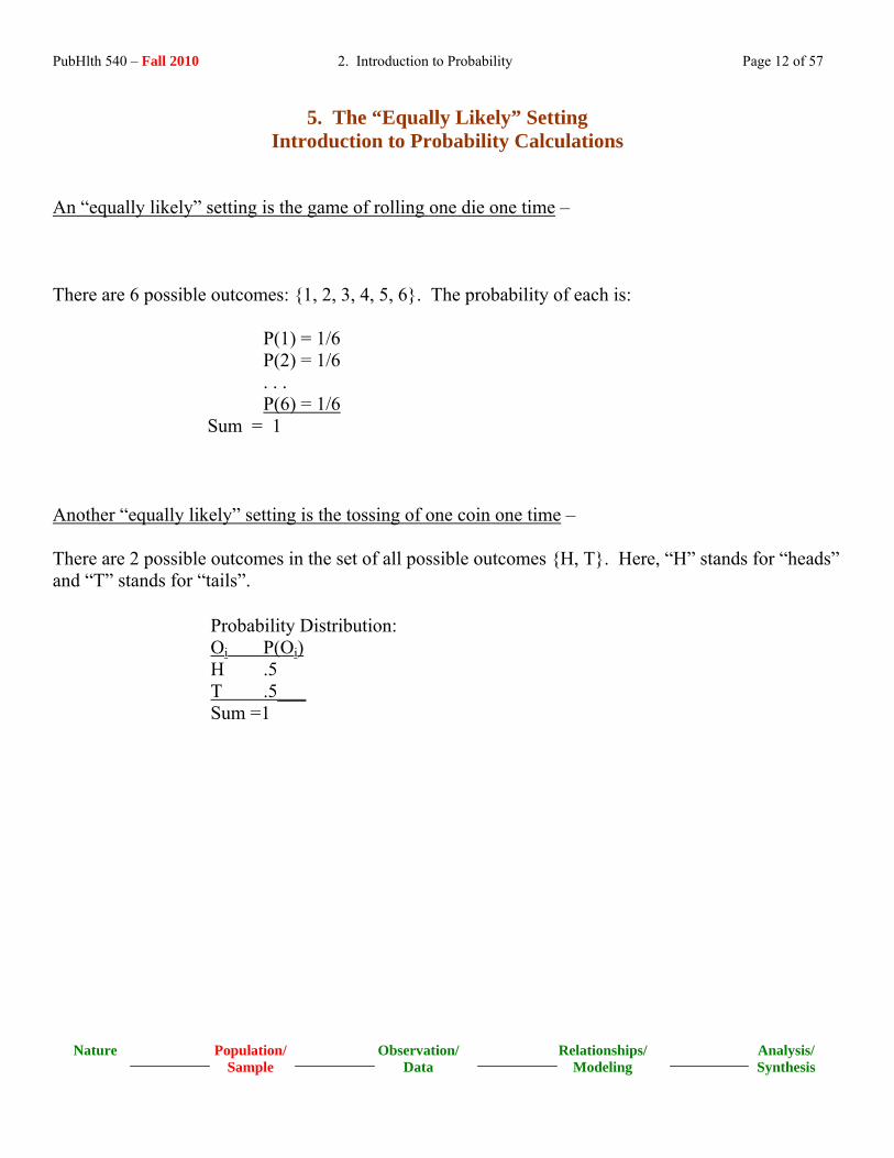
5. The “Equally Likely” Setting Introduction to Probability Calculations

An “equally likely” setting is the game of rolling one die one time – There are 6 possible outcomes: {1, 2, 3, 4, 5, 6}. The probability of each is:

P(1) = 1/6 P(2) = 1/6 . . . P(6) = 1/6

Sum = 1

Another “equally likely” setting is the tossing of one coin one time – There are 2 possible outcomes in the set of all possible outcomes {H, T}. Here, “H” stands for “heads” and “T” stands for “tails”.

Probability Distribution: Oi P(Oi) H .5 T .5___ Sum =1


Nature Sample

Observation/ Data


Analysis/ Synthesis

Population/

Here is another “equally likely” setting – The set of all possible samples of digits of sample size n that can be taken, with replacement, from a population of size N. E.g., for N=3, n=2: Sample Space: S = { (1,1), (1,2), (1,3), (2,2), (2,1), (2,3), (3,1), (3,2), (3,3) } Probability Model: Assumption: equally likely outcomes, with Nn = 32 = 9 outcomes

Probability Distribution: Outcome, Oi P(Oi) (1,1) 1/9 (1,2) 1/9 … … (3,3) 1/9___ Sum =1

Note – More on the ideas of “with replacement” and “without replacement” later. Another “equally likely” setting – Toss 2 coins Set of all possible outcomes: S = {HH, HT, TH, TT}

Probability Distribution: Outcome, Oi P(Oi) HH ¼ = .25 HT ¼ = .25 TH ¼ = .25 TT ¼ = .25 Sum =1


Nature Sample

Observation/ Data


Analysis/ Synthesis

Population/

Introduction to Events “E” – Recall that an event can be a set of elementary outcomes. The probability of each event is the simple addition of the probabilities of the qualifying elementary outcomes: Event , E Set of Qualifying Outcomes, O P(Ei) E1: 2 heads {HH} ¼ = .25 E2: Just 1 head {HT, TH} ¼ + ¼ = .50 E3: 0 heads {TT} ¼ = .25 E4: Both the same {HH, TT} ¼ + ¼ = .50 E5: At least 1 head {HH, HT, TH} ¼ + ¼ + ¼ = .75 Soon, we will learn when we can simply add probabilities and when we cannot; the answer has to do with the idea of “mutually exclusive” which is introduced on page 19. Another Example - Calculation of a Composite Event in An “Equally Likely” Setting – Recall the set of all possible samples of size n=2 that can be taken, with replacement, from a population of size N=3: Sample Space S of all possible elementary outcomes O: S = { (1,1), (1,2), (1,3), (2,2), (2,1), (2,3), (3,1), (3,2), (3,3) } Probability Model: Each outcome is equally likely and is observed with probability 1/9

Probability Distribution: Outcome, Oi P(Oi) (1,1) 1/9 (1,2) 1/9 … … (3,3) 1/9___ Sum =1


Nature Sample

Observation/ Data


Analysis/ Synthesis

Population/

Suppose we are interested in the event that subject “2” is in our sample. Thus, E: subject 2 is in the sample. S={ (1,1), (1,2), (1,3), (2,1), (2,2), (2,3), (3,1), (3,2), (3,3) } By the “red underlines” (or just “underlines” if you don’t see the red), we notice that the event of interest occurs in 5 of the 9 equally likely samples Pr{ E } = Pr { (1,2), (2,1), (2,2), (2,3), (3,2) } = 1/9 + 1/9 + 1/9 + 1/9 + 1/9 = 5/9 = .56 We have what we need to define the associated probability distribution.

1. Sample Space

2. Elementary Outcomes or Sample Points

3. Events


Nature Sample

Observation/ Data


Analysis/ Synthesis

Population/

6. Some Useful Basics

6a. Sample Space, Elementary Outcomes, Event Population or Sample Space - The population or sample space is defined as the set of all possible outcomes of a random variable. Example – The sexes of the first and second of a pair of twins. The population or sample space of all possible outcomes “O” is therefore:

{ boy, boy } { boy, girl } { girl, boy } { girl, girl },

The first sex is that of the first individual in the pair while the second sex is that of the second individual in the pair.

NOTE: This random variable is a little different than most of the random variables described so far. Here, specification of one outcome requires two pieces of information (the sex of the first individual and the sex of the second individual) instead of one piece of information. It is an example of a bivariate random variable.


Nature Sample

Observation/ Data


Analysis/ Synthesis

Population/

Elementary Outcome (Sample Point), O – One sample point corresponds to each possible outcome “O” of a random variable. Such single points are elementary outcomes. Example – For the twins example, a single sample (elementary) point is: { boy, girl } There are three other single sample (elementary) points: { girl, boy }, { girl, girl }, and { boy, boy }. Event - An event “E” is a collection of individual outcomes “O”. Notice that the individual outcomes or elementary sample points are denoted O1, O2, … while events are denoted E1, E2, … Example – Consider again the random variable defined as the sexes of the first and second individuals in a pair of twins. Consider, in particular, the event defined “boy”. The set of outcomes defined by this event is the collection of all possible ways in which a pair of twins can include a boy. There are three such ways:

{ boy, boy } { boy, girl } { girl, boy }


Nature Sample

Observation/ Data


Analysis/ Synthesis

Population/

Probability - For now, we are considering a discrete probability distribution setting. Here, the probability of an event is the relative frequency with which (“chances of”) at least one outcome of the event occurs in the population. If an event is denoted by E, then the probability that the event E occurs is written as P(E). Example – For the twins example, we might be interested in three events: E1 = “two boys”, E2 = “two girls”, E3 = “one boy, one girl”. Assume that the chances of each sex are 1/2 for both the first and second twin and that the sex of the second twin is not determined in any way by the sex of the first twin. A table summarizing the individual probabilities of these events is: Event Description Probability of Event E1 “two boys” Prob{1st=boy}Prob{2nd=boy} = {boy,boy} (1/2) x (1/2) = 1/4 = 0.25 E2 “two girls” Prob{1st=girl}Prob{2nd=girl} = {girl,girl} (1/2) x (1/2) = 1/4 = 0.25 E3 “one boy, one girl” Prob{1st=girl}Prob{2nd=boy} + {girl,boy} OR Prob{1st=boy}Prob{2nd=girl} = {boy,girl} (1/2) x (1/2) = 1/4 = 0.25 + (1/2) x (1/2) = 1/4 = 0.25 = 0.50


Nature Sample

Observation/ Data


Analysis/ Synthesis

Population/

6b. “Mutually Exclusive” and “Statistical Independence” Explained

The ideas of mutually exclusive and independence are different. The ways we work with them are also different. Tip – The distinction can be appreciated by incorporating an element of time. Mutually Exclusive (“cannot occur at the same time”) - Here’s an example that illustrates the idea. A coin toss cannot produce heads and tails simultaneously. A coin landed “heads” excludes the possibility that the coin landed “tails”. We say the events of “heads” and “tails” in the outcome of a single coin toss are mutually exclusive. Two events are mutually exclusive if they cannot occur at the same time. Every day Examples of Mutually Exclusive –

• Weight of an individual classified as “underweight”, “normal”, “overweight”

• Race/Ethnicity of an individual classified as “White Caucasian”, “African American”, “Latino”, “Native African”, “South East Asian”, “Other”

• Gender of an individual classified as “Female”, “Male”, “Transgender” One More Example of Mutually Exclusive – For the twins example introduced previously, the events E1 = “two boys” and E2 = “two girls” are mutually exclusive.


Nature Sample

Observation/ Data


Analysis/ Synthesis

Population/

Statistical Independence - Tip - Think time. Think about things occurring chronologically in time. To appreciate the idea of statistical independence, imagine you have in front of you two outcomes that you have observed. Eg.-

• Individual is male with red hair.

• Individual is young in age with high blood pressure.

• First coin toss yields “heads” and second coin toss yields “tails”. Two events are statistically independent if the chances, or likelihood, of one event is in no way related to the likelihood of the other event. A familiar example of statistical independence corresponds to third example here - the first coin toss yielding heads and the second toss yielding tails. Under the assumption that the coin is “fair”, we say The outcomes on the first and second coin tosses are statistically independent and, therefore, probability [“heads” on 1st and “tails” on 2nd ] = (1/2)(1/2) = 1/4. Thus, the distinction between “mutually exclusive” and “statistical independence” can be appreciated by incorporating an element of time. Mutually Exclusive (“cannot occur at the same time”) “heads on 1st coin toss” and “tails on 1st coin toss” are mutually exclusive. Probability [“heads on 1st” and “tails on 1st” ] = 0 Statistical Independence (“the first does not influence the occurrence of the later 2nd”) “heads on 1st coin toss” and “tails on 2nd coin toss” are statistically independent Probability [“heads on 1st” and “tails on 2nd ” ] = (1/2) (1/2)


Nature Sample

Observation/ Data


Analysis/ Synthesis

Population/

SO … BE CAREFUL !! The concepts of mutually exclusive and independence are distinct and in no sense equivalent. To see this: For A and B independent “one does not influence the other” Pr(A and B) = P(A) P(B) E.g. A=red hair B=winning the lottery For A and B mutually exclusive: “cannot occur at the same time” Pr(A and B) = Pr (empty event) = 0 E.g. A=lottery winning is $10 B=lottery game not played


Nature Sample

Observation/ Data


Analysis/ Synthesis

Population/

6c. Complement, Union, Intersection Complement (“opposite”, “everything else”) - The complement of an event E is the event consisting of all outcomes in the population or sample space that are not contained in the event E. The complement of the event E is denoted using a superscript c, as in Ec . Example – For the twins example, consider the event E1 = “two boys”. The complement of the event E1 is E1

c = { boy, girl }, { girl, boy }, { girl, girl } Union, A or B (“either or”) - The union of two events, say A and B, is another event which contains those outcomes which are contained either in A or in B. The notation used is A ∪ B.


Example – For the twins example suppose event “A” is defined { boy, girl } and event “B” is defined { girl, boy }. The union of events A and B is: A ∪ B = { boy, girl }, { girl, boy } Intersection, A and B (“only the common part”) - The intersection of two events, say A and B, is another event which contains only those outcomes which are contained in both A and in B. The notation used is A ∩ B. Here it is depicted in the color gray.

Example – For the twins example, consider next the events E1 defined as “having a boy” and E2 defined as “having a girl”. Thus, E1 = { boy, boy }, { boy, girl }, { girl, boy } E2 = { girl, girl }, { boy, girl }, { girl, boy } These two events do share some common outcomes. The intersection of E1 and E2 is “having a boy and a girl”:

E1 ∩ E2 = { girl, boy }, { boy, girl }

Nature Sample

Observation/ Data


Analysis/ Synthesis

Population/


Nature Sample

Observation/ Data


Analysis/ Synthesis

Population/

7. Independence, Dependence, and Conditional Probability

Recall the illustration of statistical independence in the twins example – The sex of the second twin was not determined in any way by the sex of the first twin. This is what is meant by independence. The idea of dependence - The occurrence of a first event alters, at least in part, the occurrence of a second event. Another Wording of Statistical Independence - Two events A and B are mutually independent if the chances, or likelihood, of one event is in no way related to the likelihood of the other event. When A and B are mutually independent: P(A and B) = P(A) P(B) Example – Event A = “a woman is hypertensive” Event B = “her mother-in-law is hypertensive”. The assumption of independence seems reasonable since the two women are not genetically related. If the probability of being hypertensive is 0.07 for each woman, then the probability that BOTH the woman and her mother-in-law are hypertensive is: P(A and B) = P(A) x P(B) = 0.07 x 0.07 = 0.0049


Nature Sample

Observation/ Data


Analysis/ Synthesis

Population/

Dependence - Two events are dependent if they are not independent. The probability of both occurring depends on the outcome of at least one of the two. Two events A and B are dependent if the probability of one event is related to the probability of the other: P(A and B) ≠ P(A) P(B) Example - An offspring of a person with Huntington’s Chorea has a 50% chance of contracting Huntington’s Chorea. This is tantamount to saying “If it is given that a person has Huntington’s Chorea, then the chances of his/her offspring having the disease is 50%” Let Event A = “parent has Huntington’s Chorea” Let Event B = “offspring has Huntington’s Chorea”. Without knowing anything about the parent’s family background, suppose the chances that the parent has Huntington’s Chorea is 0.0002. Suppose further that, if the parent does not have Huntington’s Chorea, the chances that the offspring has Huntington’s Chorea is 0.000199. However, if the parent has Huntington’s Chorea, the chances that the offspring has Huntington’s Chorea jumps to 0.50. Thus, the chances that both have Huntington’s Chorea is not simply 0.0002 x 0.000199. That is, P(A and B) ≠ P(A) x P(B) It is possible to calculate P(A and B), but this requires knowing how to relate P(A and B) to conditional probabilities. This is explained below.


Conditional Probability (“what happened first is assumed”) - Conditional probability refers to the probability of an event, given that another event is known to have occurred. We do these sorts of calculations all the time. As we’ll see later in this course and in BE640, we might use the estimation of conditional probabilities when it is of interest to assess how dependent two events are, relative to each other.

The conditional probability that event B has occurred given that event A has occurred is denoted P(B|A) and is defined

P(B|A) = P(A and B)P(A)

provided that P(A) ≠ 0.

Hint - When thinking about conditional probabilities, think in stages. Think of the two events A and B occurring chronologically, one after the other, either in time or space. Example - Huntington’s Chorea again ♣ The conditional probability that an offspring has Huntington’s Chorea given a parent has

Huntington’s Chorea is 0.50. ♣ It is also known that the parent has Huntington’s Chorea with probability 0.0002. ♣ Consider A = event that parent has Huntington’s Chorea B = event that offspring has Huntington’s Chorea ♣ Thus, we know Pr (A) = 0.0002 Pr (B|A) = 0.5

Nature Sample

Observation/ Data


Analysis/ Synthesis

Population/


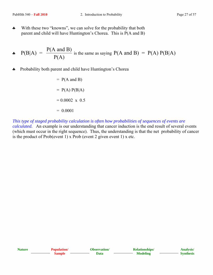
♣ With these two “knowns”, we can solve for the probability that both parent and child will have Huntington’s Chorea. This is P(A and B)

♣ P(B|A) = P(A and B)P(A)

is the same as saying P(A and B) = P(A) P(B|A)

♣ Probability both parent and child have Huntington’s Chorea = P(A and B) = P(A) P(B|A) = 0.0002 x 0.5 = 0.0001 This type of staged probability calculation is often how probabilities of sequences of events are calculated. An example is our understanding that cancer induction is the end result of several events (which must occur in the right sequence). Thus, the understanding is that the net probability of cancer is the product of Prob(event 1) x Prob (event 2 given event 1) x etc.

Nature Sample

Observation/ Data


Analysis/ Synthesis

Population/


Nature Sample

Observation/ Data


Analysis/ Synthesis

Population/

8. Some Useful Tools for Calculating Probabilities 8a. The Addition Rule A tool for calculating the probability of “either or both” of two events

Consider the following

Event A: Go to Starbucks. Play the game A. A win produces a latte. Suppose A yields win with probability = 0.15 Event B: Next go to Dunkin Donuts. Play the game B . A win produces a donut. Suppose B yields “win” with probability = 0.35

The Addition Rule For two events, say A and B, the probability of an occurrence of either or both is written Pr [A ∪ B ] and is Pr [A ∪ B ] = Pr [ A ] + Pr [ B ] - Pr [ A and B ] Notice what happens to the addition rule if A and B are mutually exclusive! Pr [A ∪ B ] = Pr [ A ] + Pr [ B ] Example – In the scenario above, assume that the games offered by Starbucks and Dunkin Donuts are statistically independent. This means that Pr [ A ] = Pr [ latte ] = 0.15 Pr [ B ] = Pr [ donut ] = 0.35 Pr [ A and B ] = Pr [ latte & donut ] = (0.15)(0.35) = 0.0525 We can use the addition rule to obtain the probability of winning a latte or a donut. Pr [ latte or donut ] = Pr [A ∪ B ] = Pr [ A ] + Pr [ B ] - Pr [ A and B ] = 0.15 + 0.35 - 0.0525 = 0.4475


Nature Sample

Observation/ Data


Analysis/ Synthesis

Population/

8b. The Multiplication Rule A tool for calculating the probability that “both”of two events occur

We consider again the Huntington’s Chorea example and use the same scenario to illustrate the definition of the multiplication rule.

Event A: A parent has probability of Huntington’s Chorea = 0.0002 Event B|A: If it is known that a parent has Huntington’s Chorea, then the conditional probability that the offspring also has Huntington’s Chorea is = 0.50

The Multiplication Rule For two events, say A and B, the probability that both occur is written Pr [A ∩ B ] and is Pr [A ∩ B ] = Pr [ A ] x Pr [ B | A ] Example – In this scenario we have Pr [ A ] = Pr [ parent has disease ] = 0.0002 Pr [ B | A ] = Pr [ child has disease given parent does ] = 0.50 Pr [ A and B ] = Pr [ both have disease ] = (0.0002)(0.50) = 0.0001


Nature Sample

Observation/ Data


Analysis/ Synthesis

Population/

8c. Theorem of Total Probabilities A tool for calculating the probability of a sequence of events This is actually quite handy. In thinking about a sequence of events, think in stages over time – that is, from one event to the next event and then to the next event after that, and so on. Now we’ll play a game. The game has two steps. Game -

Step 1: Choose one of two games to play: G1 or G2 G1 is chosen with probability = 0.85 G2 is chosen with probability = 0.15 (notice that probabilities sum to 1) Step 2: Given that you choose a game, G1 or G2 : G1 yields “win” with conditional probability P(win|G1) = 0.01 G2 yields “win” with conditional probability P(win|G2) = 0.10

What is the overall probability of a win, Pr(win)? Hint – Think of all the distinct ( mutually exclusive) ways in which a win could occur and sum their associated probabilities. There are only two such scenarios, and each scenario involves two component events. Pr(win) = Pr[G1 chosen] Pr[win|G1] + Pr[G2 chosen] Pr[win|G2] event 1 event 2 event 1 event 2 scenario #1 scenario #2

= (.85) (.01) + (.15) (.10) = 0.0235

This intuition has a name – The Theorem of Total Probabilities.


Theorem of Total Probabilities

Suppose that a sample space S can be partitioned (carved up into bins) so that S is actually a union that looks like S = G G G1 2U U U... K

If you are interested in the overall probability that an event “E” has occurred, this is calculated P[E] = P[G ]P[E|G ] + P[G P[E|G + ... + P[G P[E|G1 1 2 2 K K] ] ] ] provided the conditional probabilities are known.

Example – The lottery game just discussed.

G1 = Game #1 G2 = Game #2 E = Event of a win.

So what? Applications of the Theorem of Total Probabilities – We’ll see this again in this course and also in BE640

♣ Diagnostic Testing ♣ Survival Analysis

Nature Sample

Observation/ Data


Analysis/ Synthesis

Population/


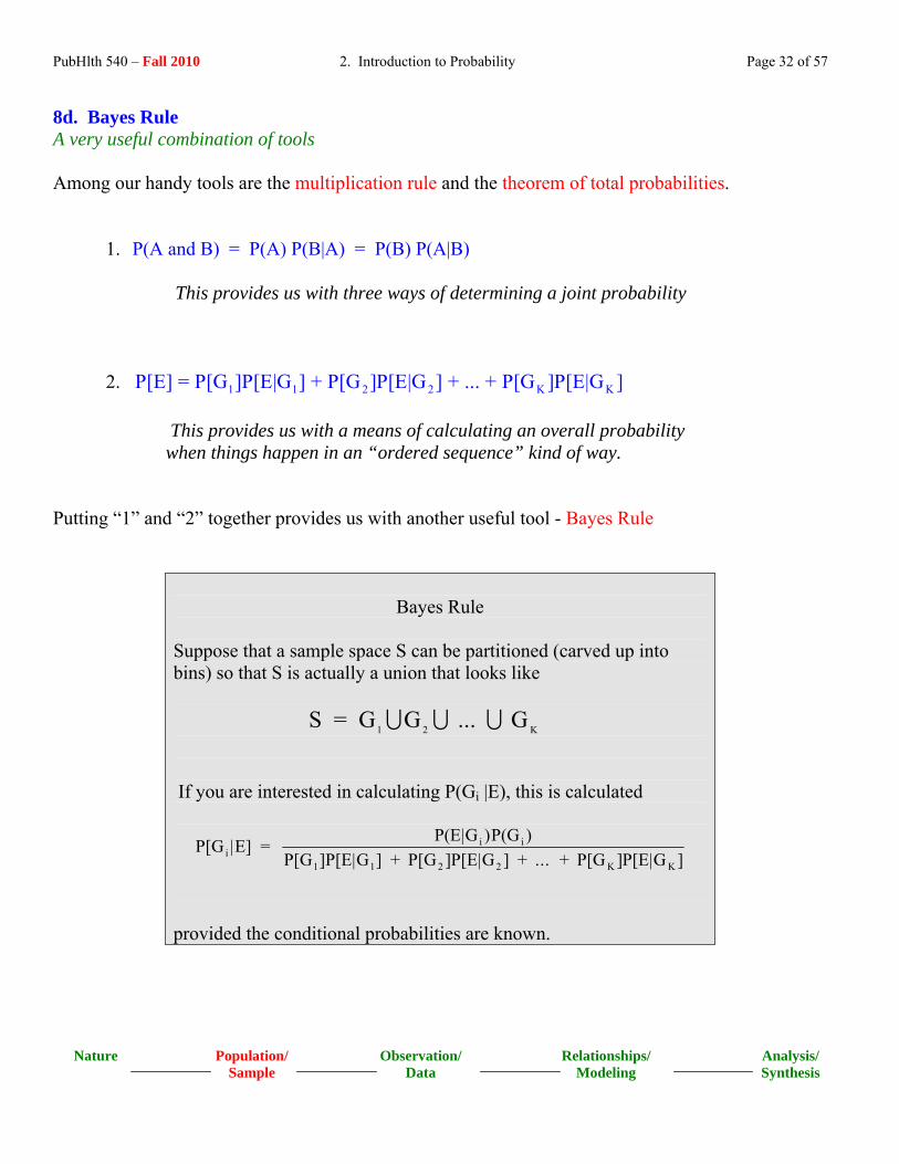
8d. Bayes Rule A very useful combination of tools Among our handy tools are the multiplication rule and the theorem of total probabilities.

1. P(A and B) = P(A) P(B|A) = P(B) P(A|B) This provides us with three ways of determining a joint probability

2. | This provides us with a means of calculating an overall probability when things happen in an “ordered sequence” kind of way.

1 1 2 2 KP[E] = P[G ]P[E|G ] + P[G ]P[E|G ] + ... + P[G ]P[E KG ]

Putting “1” and “2” together provides us with another useful tool - Bayes Rule

Bayes Rule

Suppose that a sample space S can be partitioned (carved up into bins) so that S is actually a union that looks like S = G G G1 2U U U... K

If you are interested in calculating P(Gi |E), this is calculated

P[G |E] = P(E|G P(G

P[G ]P[E|G ] + P[G P[E|G + ... + P[G P[E|Gii i

1 1 2 2 K

) )] ] ] K ]

provided the conditional probabilities are known.

Nature Sample

Observation/ Data


Analysis/ Synthesis

Population/


Illustration of a Bayes Theorem Application

Source: http://yudkowsky.net/bayes/bayes.html You’ll find a link to this URL on the course website page for 2. Introduction to Probability. This URL is reader friendly.

• Suppose it is known that the probability of a positive mammogram is 80% for women with breast cancer and is 9.6% for women without breast cancer.

• Suppose it is also known that the likelihood of breast cancer is 1%

• If a women participating in screening is told she has a positive mammogram, what are the chances that she has breast cancer disease?

Let

• A = Event of breast cancer • X = Event of positive mammogram

What we want to calculate is Probability (A | X) What we have as available information is

• Probability (X | A) = .80 Probability (A) = .01 • Probability (X | not A) = .096 Probability (not A) = .99

Here’s how the solution works …

Pr(A and X)Pr( A | X ) = Pr (X)

by definition of conditional Probability

Pr(X | A) Pr(A)=

Pr(X) because we can re-write the numerator this way

Pr(X | A) Pr(A)=

Pr(X | A) Pr(A) + Pr(X | not A) Pr(not A) by thinking in steps in denominator

(.80) (.01)=

(.80) (.01) + (.096) (.99) = .078 , representing a 7.8% likelihood.

Nature Sample

Observation/ Data


Analysis/ Synthesis

Population/

http://yudkowsky.net/bayes/bayes.html


Nature Sample

Observation/ Data


Analysis/ Synthesis

Population/

9. A Simple Probability Model: The Bernoulli Distribution

The Bernoulli Distribution is an example of a discrete probability distribution. It is an appropriate tool for the analysis of proportions and rates. Recall the coin toss. “50-50 chance of heads” can be re-cast as a random variable. Let Z = random variable representing outcome of one toss, with Z = 1 if “heads” 0 if “tails” π= Probability [ coin lands “heads” }. Thus,

π = Pr [ Z = 1 ] We have what we need to define a discrete probability distribution. Ingredient 1 Enumeration of all possible outcomes

- outcomes are mutually exclusive - outcomes are exhaust all possibilities

1 0

Ingredient 2 Associated probabilities of each - each probability is between 0 and 1 - sum of probabilities totals 1

Outcome Pr[outcome]

0 (1 - π) 1 π


Nature Sample

Observation/ Data


Analysis/ Synthesis

Population/

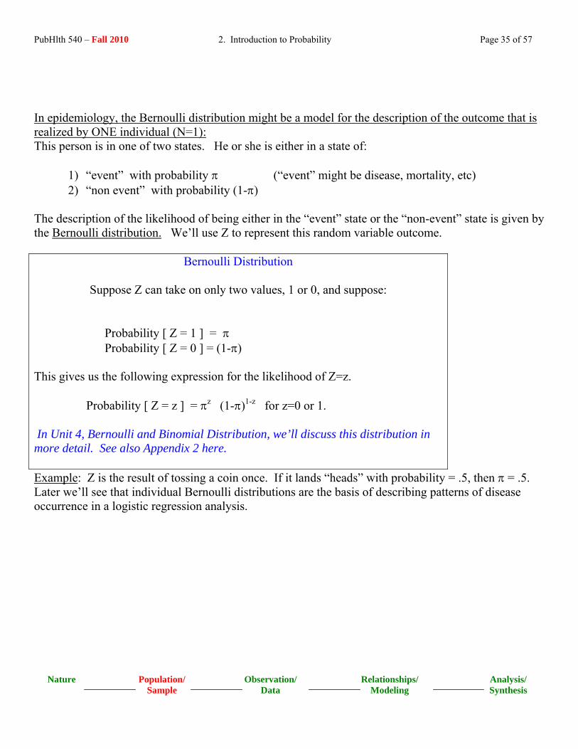
In epidemiology, the Bernoulli distribution might be a model for the description of the outcome that is realized by ONE individual (N=1): This person is in one of two states. He or she is either in a state of:

1) “event” with probability π (“event” might be disease, mortality, etc) 2) “non event” with probability (1-π)

The description of the likelihood of being either in the “event” state or the “non-event” state is given by the Bernoulli distribution. We’ll use Z to represent this random variable outcome.

Bernoulli Distribution

Suppose Z can take on only two values, 1 or 0, and suppose: Probability [ Z = 1 ] = π Probability [ Z = 0 ] = (1-π) This gives us the following expression for the likelihood of Z=z. Probability [ Z = z ] = πz (1-π)1-z for z=0 or 1. In Unit 4, Bernoulli and Binomial Distribution, we’ll discuss this distribution in more detail. See also Appendix 2 here. Example: Z is the result of tossing a coin once. If it lands “heads” with probability = .5, then π = .5. Later we’ll see that individual Bernoulli distributions are the basis of describing patterns of disease occurrence in a logistic regression analysis.


Nature Sample

Observation/ Data


Analysis/ Synthesis

Population/

10. Probability in Diagnostic Testing

Students of epidemiology are introduced to, among other things:

• concepts of diagnostic testing (sensitivity, specificity, predictive value positive, predictive value negative);

• concepts of disease occurrence (prevalence, incidence); and • measures of association for describing exposure-disease relationships (risk, odds, relative

risk, odds ratio).

These have their origins in notions of conditional probability. 10 a. Prevalence ("existing") The point prevalence of disease is the proportion of individuals in a population that has disease at a single point in time (point), regardless of the duration of time that the individual might have had the disease. Prevalence is NOT a probability. Example - A study of sex and drug behaviors among gay men is being conducted in Boston, Massachusetts. At the time of enrollment, 30% of the study cohort were sero-positive for the HIV antibody. Rephrased, the point prevalence of HIV sero-positivity was 0.30 at baseline. 10 b. Cumulative Incidence ("new") The cumulative incidence of disease is the probability an individual who did not previously have disease will develop the disease over a specified time period. Example - Consider again Example 1, the study of gay men and HIV sero-positivity. Suppose that, in the two years subsequent to enrollment, 8 of the 240 study subjects sero-converted. This represents a two year cumulative incidence of 8/240 or 3.33%.


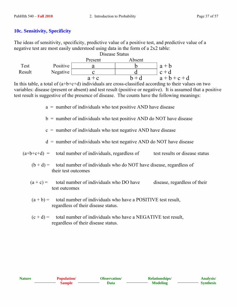
10c. Sensitivity, Specificity The ideas of sensitivity, specificity, predictive value of a positive test, and predictive value of a negative test are most easily understood using data in the form of a 2x2 table: Disease Status Present Absent

Test Positive a b a + b Result Negative c d c + d

a + c b + d a + b + c + d In this table, a total of (a+b+c+d) individuals are cross-classified according to their values on two variables: disease (present or absent) and test result (positive or negative). It is assumed that a positive test result is suggestive of the presence of disease. The counts have the following meanings: a = number of individuals who test positive AND have disease b = number of individuals who test positive AND do NOT have disease c = number of individuals who test negative AND have disease d = number of individuals who test negative AND do NOT have disease (a+b+c+d) = total number of individuals, regardless of test results or disease status (b + d) = total number of individuals who do NOT have disease, regardless of their test outcomes (a + c) = total number of individuals who DO have disease, regardless of their test outcomes (a + b) = total number of individuals who have a POSITIVE test result, regardless of their disease status. (c + d) = total number of individuals who have a NEGATIVE test result, regardless of their disease status.

Nature Sample

Observation/ Data


Analysis/ Synthesis

Population/


Sensitivity Among those persons who are known to have disease, what are the chances that the diagnostic test will yield a positive result? To answer this question requires restricting attention to the subset of (a+c) persons who actually have disease. The number of persons in this subset is (a+c). Among this "restricted total" of (a+c), it is observed that “a” test positive.

sensitivity = aa + c

Sensitivity is a conditional probability. It is the conditional probability that the test suggests disease given that the individual has the disease. For E1=event that individual has disease and E2=event that test suggests disease: sensitivity = P(E2 | E1 ) To see that this is equal to what we think it should be, ( a / [a+c] ), use the definition of conditional probability:

P(E E P(E and EP(E2 12 1

1

| ) ))

=

=a / (a + b + c + d)

(a + c) / (a + b + c + d)

= LNMOQP

a(a + c)

, which matches.

Unfortunately, “sensitivity” also goes by other names: * positivity in disease * true positive rate

Nature Sample

Observation/ Data


Analysis/ Synthesis

Population/


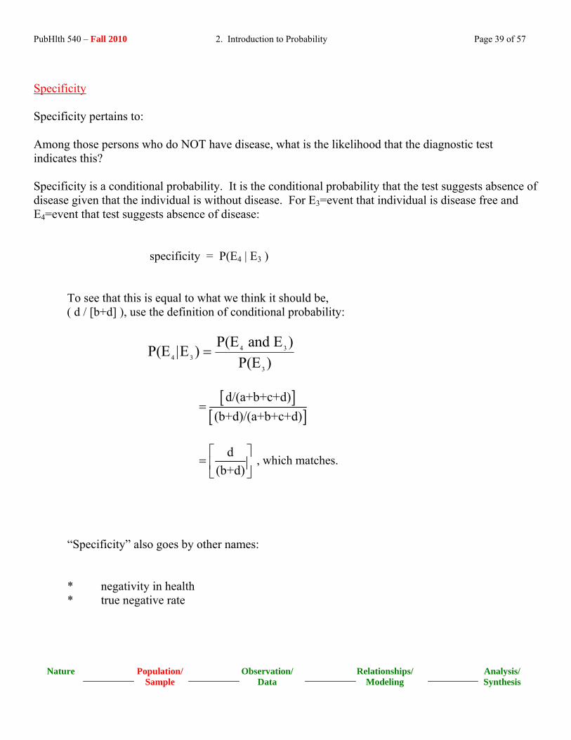
Specificity Specificity pertains to: Among those persons who do NOT have disease, what is the likelihood that the diagnostic test indicates this? Specificity is a conditional probability. It is the conditional probability that the test suggests absence of disease given that the individual is without disease. For E3=event that individual is disease free and E4=event that test suggests absence of disease: specificity = P(E4 | E3 ) To see that this is equal to what we think it should be, ( d / [b+d] ), use the definition of conditional probability:


3

| ) ))

=

[ ]

[ ]d/(a+b+c+d)

(b+d)/(a+b+c+d)=

d

(b+d)⎡ ⎤

= ⎢⎣ ⎦

⎥ , which matches.

“Specificity” also goes by other names: * negativity in health * true negative rate

Nature Sample

Observation/ Data


Analysis/ Synthesis

Population/


10 d. Predictive Value Positive, Negative Sensitivity and specificity are not very helpful in the clinical setting.

♦ We don’t know if the patient has disease (a requirement for sensitivity, specificity calculations).

♦ This is what we are wanting to learn. ♦ Thus, sensitivity and specificity are not the calculations performed

in the clinical setting (they’re calculated in the test development setting). Of interest to the clinician: “For the person who is found to test positive, what are the chances that he or she truly has disease?".

♦ This is the idea of “predictive value positive test” "For the person who is known to test negative, what are the chances that he or she is truly disease free?".

♦ This is the idea of “predictive value negative test” Predictive Value Positive Test Among those persons who test positive for disease, what is the relative frequency of disease? Predictive value positive test is also a conditional probability. It is the conditional probability that an individual with a test indicative of disease actually has disease. Attention is restricted to the subset of the (a+b) persons who test positive. Among this "restricted total" of (a+b),

Predictive value positive = aa + b

Nature Sample

Observation/ Data


Analysis/ Synthesis

Population/


Other Names for "Predictive Value Positive Test": * posttest probability of disease given a positive test * posterior probability of disease given a positive test Also of interest to the clinician: Will unnecessary care be given to a person who does not have the disease? Predictive Value Negative Test Among those persons who test negative for disease, what is the relative frequency of absence of disease? Predictive value negative test is also a conditional probability. It is the conditional probability that an individual with a test indicative of NO disease is actually disease free. Attention is restricted to the subset of the (c+d) persons who test negative. Among this "restricted total" of (c+d),

Predictive value negative = dc + d

Other Names for "Predictive Value Negative Test": * posttest probability of NO disease given a negative test * posterior probability of NO disease given a negative test

Nature Sample

Observation/ Data


Analysis/ Synthesis

Population/


11. Probability and Measures of Association for the 2x2 Table

Epidemiologists and public health researchers are often interested in exploring the relationship between a yes/no (dichotomous) exposure variable and a yes/no (dichotomous) disease outcome variable. A 2x2 summary table is again useful. Disease Status Present Absent

Exposed a b a + b Not c d c + d

a + c b + d a + b + c + d (a+b+c+d) = total number of individuals, regardless of exposure or disease status (b + d) = total number of individuals who do NOT have disease, regardless of their exposure status (a + c) = total number of individuals who DO have disease, regardless of their exposure status (a + b) = total number of individuals who have a POSITIVE exposure, regardless of their disease status. (c + d) = total number of individuals who have a NO exposure, regardless of their disease status. 11a. Risk ("simple probability") Risk of disease, without referring to any additional information, is simply the probability of disease. An estimate of the probability or risk of disease is provided by the relative frequency:

(a + c)

(a + b + c + d)

Nature Sample

Observation/ Data


Analysis/ Synthesis

Population/


Typically, however, conditional risks are reported. For example, if it were of interest to estimate the risk of disease for persons with a positive exposure status, then attention would be restricted to the (a+b) persons positive on exposure. For these persons only, it seems reasonable to estimate the risk of disease by the relative frequency: The straightforward calculation of the risk of disease for the persons known to have a positive exposure status is:

P(Disease among Exposed) = a(a + b)

Repeating the calculation using the definition of conditional probability yields the same answer. Let E1 =event of positive exposure and E2=event of disease. Then: Risk (disease given POSITIVE exposure) =


1

| ) ))

=

=a / (a + b + c + d)

(a + b) / (a + b + c + d)

= LNMOQP

a(a + b)

, which matches.

Nature Sample

Observation/ Data


Analysis/ Synthesis

Population/


11b. Odds("comparison of two complementary (opposite) outcomes"): In words, the odds of an event "E" is the chances of the event occurring in comparison to the chances of the same event NOT occurring.

c

Pr(Event occurs) P(E) P(E)Odds = Pr(Event does NOT occur) 1 -P(E) (E )

= =

Example - Perhaps the most familiar example of odds is reflected in the expression "the odds of a fair coin landing heads is 50-50". This is nothing more than:

Odds(heads) = P(heads)P(heads

P(heads)P(tails)

.50

.50c )= =

Similarly, for the exposure-disease data in the 2x2 table,

Odds(disease) = P(disease)P(disease

P(disease)P(NO disease)

(a + c) / (a + b + c + d)(b + d) / (a + b + c + d)

(a + c)(b + d)c )

= = =

Odds(exposed) = P(exposed)P(exposed

P(exposed)P(NOT exposed)

(a + b) / (a + b + c + d)(c + d) / (a + b + c + d)

(a + b)(c + d)c )

= = =

Nature Sample

Observation/ Data


Analysis/ Synthesis

Population/


What if it is suspected that exposure has something to do with disease? In this setting, it might be more meaningful to report the odds of disease separately for persons who are exposed and persons who are not exposed. Now we’re in the realm of conditional odds.

Odds(disease | exposed) = Pr(disease|exposed)Pr(NO disease|exposed)

a / (a + b)b / (a + b)

ab

= =

Odds(disease | NOT exposed) = Pr(disease|not exposed)Pr(NO disease|not exposed)

c / (c + d)d / (c + d)

cd

= =

Notice the vertical bar in expressions such as odds(disease|exposed). This vertical bar is nothing more than a “secretarial” shorthand that communicates a conditioning. Translation: “odds of disease given that exposure is present” Similarly, one might calculate the odds of exposure separately for diseased persons and NON-diseased persons:

Odds(exposed | disease) = Pr(exposed|disease)Pr(NOT exposed|disease)

a / (a + c)c / (a + c)

ac

= =

Odds(exposed | NO disease) = Pr(exposed|NO disease)Pr(NOT exposed|NO disease)

b / (b + d)d / (b + d)

bd

= =

Nature Sample

Observation/ Data


Analysis/ Synthesis

Population/


Nature Sample

Observation/ Data


Analysis/ Synthesis

Population/

11c. Relative Risk("comparison of two conditional probabilities") Various epidemiological studies (prevalence, cohort, case-control designs) give rise to data in the form of counts in a 2x2 table.

Suppose we are interested in exploring the association between exposure and disease.

Recall our 2x2 table.

Disease Healthy Exposed a b a+b Not exposed c d c+d a+c b+d a+b+c+d Let’s consider some actual counts, specifically 310 persons cross-classified by exposure and disease:

Disease Healthy Exposed 2 8 10 Not exposed 10 290 300 12 298 310 We might have more than one 2x2 table if the population of interest is partitioned into subgroups or strata. Example: Stratification by gender would yield a separate 2x2 table for men and women.


Relative Risk The relative risk is the ratio of the conditional probability of disease among the exposed to the conditional probability of disease among the non-exposed. Relative Risk: The ratio of two conditional probabilities

RR = a / (a + b)c / (c + d)

Example: In our 2x2 table, we have a/(a+b) = 2/10 = .20, c/(c+d) = 10/300 = .0333 Thus, RR = .20 / .0333 = 6.006 • It has been found empirically that many exposure-disease relationships vary with age in such a way that the log linear model is a good description. Specifically, the change with age in the relative risk of disease with exposure is reasonably stable. In such instances, the model is preferable to an additive risk model.

Nature Sample

Observation/ Data


Analysis/ Synthesis

Population/


11 d. Odds Ratio The odds ratio measure of association has some wonderful advantages, both biological and analytical. Recall first the meaning of an “odds”: Recall that if p = Probability[event] then Odds[Event] = p/(1-p) Let’s look at the odds that are possible in our 2x2 table:

Disease Healthy Exposed a b a+b Not exposed c d c+d a+c b+d a+b+c+d

Odds of disease among exposed = a/(a+b) a 2= = =.25b/(a+b) b 8⎡ ⎤⎢ ⎥⎣ ⎦

(“cohort” study)

Odds of disease among non exposed = c/(c+d) c 10= = =.0345d/(c+d) d 290⎡ ⎤⎢ ⎥⎣ ⎦

(“cohort”)

Odds of exposure among diseased = a/(a+c) a 2= = =.20c/(a+c) c 10⎡ ⎤⎢ ⎥⎣ ⎦

(“case-control”)

Odds of exposure among healthy = b/(b+d) b 8= = =.0276d/(b+d) d 290⎡ ⎤⎢ ⎥⎣ ⎦

(“case-control”)

Nature Sample

Observation/ Data


Analysis/ Synthesis

Population/


Nature Sample

Observation/ Data


Analysis/ Synthesis

Population/

Students of epidemiology learn the following great result! Odds ratio In a cohort study: OR = Odds disease among exposed = a/b = ad Odds disease among non-exposed c/d bc In a case-control study: OR = Odds exposure among diseased = a/c = ad Odds exposure among healthy b/d bc Terrific! The OR is the same, regardless of the study design, cohort (prospective) or case-control (retrospective) Note: Come back to this later if this is too “epidemiological”! Example: In our 2x2 table, a =2, b=8, c=10, and d=290 so the OR = 7.25. This is slightly larger than the value of the RR = 6.006.


Nature Sample

Observation/ Data


Analysis/ Synthesis

Population/

Thus, there are advantages of the Odds Ratio, OR. 1. Many exposure disease relationships are described better using ratio measures of association rather than difference measures of association. 2. ORcohort study = ORcase-control study

3. The OR is the appropriate measure of association in a case-control study.

- Note that it is not possible to estimate an incidence of disease in a retrospective study. This is because we select our study persons based on their disease status.

4. When the disease is rare, ORcase-control ≈ RR


Appendix 1

Some Elementary Laws of Probability

A. Definitions:

1) One sample point corresponds to each possible outcome of a random variable. 2) The sample space (some texts do use term population) consists of all sample points. 3) A group of events is said to be exhaustive if their union is the entire sample space or population. Example - For the variable SEX, the events "male" and "female" exhaust all possibilities. 4) Two events A and B are said to be mutually exclusive or disjoint if their intersection is the empty set. Example, one cannot be simultaneously "male" and "female". 5) Two events A and B are said to be complementary if they are both mutually exclusive and exhaustive. 6) The events E1, E2, ..., En are said to partition the sample space or population if: (i) Ei is contained in the sample space, and (ii) The event (Ei and Ej) = empty set for all i ≠ j; (iii) The event (E1 or E2 or ... or En) is the entire sample space or population. In words: E1, E2, ..., En are said to partition the sample space if they are pairwise mutually exclusive and together exhaustive.

Nature Sample

Observation/ Data


Analysis/ Synthesis

Population/


Nature Sample

Observation/ Data


Analysis/ Synthesis

Population/

7) If the events E1, E2, ..., En partition the sample space such that P(E1) = P(E2) = ... P(En), then: (i) P(Ei) = 1/n, for all i=1,...,n. This means that (ii) the events E1, E2, ..., En are equally likely. 8) For any event E in the sample space: 0 <= P(E) <= 1. 9) P(empty event) = 0. The empty event is also called the null set. 10) P(sample space) = P(population) = 1. 11) P(E) + P(Ec) = 1


B. Addition of Probabilities - 1) If events A and B are mutually exclusive: (i) P(A or B) = P(A) + P(B) (ii) P(A and B) = 0 2) More generally: P(A or B) = P(A) + P(B) - P(A and B) 3) If events E1, ..., En are all pairwise mutually exclusive: P(E1 or ... or En) = P(E1) + ... + P(En)

C. Conditional Probabilities -

1) P(B|A) = P(A and B) / P(A) 2) If A and B are independent: P(B|A) = P(B) 3) If A and B are mutually exclusive: P(B|A) = 0 4) P(B|A) + P(Bc|A) = 1 5) If P(B|A) = P(B|Ac): Then the events A and B are independent

D. Theorem of Total Probabilities - Let E1, ..., Ek be mutually exclusive events that partition the sample space. The unconditional probability of the event A can then be written as a weighted average of the conditional probabilities of the event A given the Ei; i=1, ..., k: P(A) = P(A|E1)P(E1) + P(A|E2)P(E2) + ... + P(A|Ek)P(Ek) E. Bayes Rule - If the sample space is partitioned into k disjoint events E1, ..., Ek, then for any event A:

j jj

1 1 2 2 k k

P(A|E )P(E )P(E |A)=

P(A|E )P(E )+P(A|E )P(E )+...+P(A|E )P(E )

Nature Sample

Observation/ Data


Analysis/ Synthesis

Population/


Nature Sample

Observation/ Data


Analysis/ Synthesis

Population/

Appendix 2 Introduction to the Concept of Expected Value

We’ll talk about the concept of “expected value” often; this is an introduction. Suppose you stop at a convenience store on your way home and play the lottery. In your mind, you already have an idea of your chances of winning. That is, you have considered the question “what are the likely winnings?”. Here is an illustrative example. Suppose the back of your lottery ticket tells you the following–

$1 is won with probability = 0.50 $5 is won with probability = 0.25 $10 is won with probability = 0.15 $25 is won with probability = 0.10

THEN “likely winning” = [$1](probability of a $1 ticket) + [$5](probability of a $5 ticket) + [$10](probability of a $10 ticket) + [$25](probability of a $25 ticket) =[$1](0.50) + [$5](0.25) +[$10](0.15) + [$25](0.10)

= $5.75

Do you notice that the dollar amount $5.75, even though it is called “most likely” is not actually a possible winning? What it represents then is a “long run average”.

Other names for this intuition are

♣ Expected winnings ♣ “Long range average” ♣ Statistical expectation!


Statistical Expectation for a Discrete Random Variable is the Same Idea.

For a discrete random variable X (e.g. winning in lottery) Having probability distribution as follows: Value of X, x = P[X = x] = $ 1 0.50 $ 5 0.25 $10 0.15 $25 0.10 The random variable X has statistical expectation E[X]=μ

μ = [x]P(X = x)all possible X=x ∑

Example – In the “likely winnings” example, μ = $5.75

Nature Sample

Observation/ Data


Analysis/ Synthesis

Population/


Statistical Expectation for the Bernoulli Distribution Recall from this reading the introduction to the Bernoulli distribution. We can expand this introduction to include a discussion of its statistical expectation. For Z distributed Bernoulli, we can calculate its statistical expectation. This statistical expectation has a name, the mean of the Bernoulli Distribution. It is represented as E[Z].

E[Z] = π because the following is true: E[Z] = [z]Probability[Z = z]

All possible z∑

= [0]Pr[Z = 0] +[1] + Pr[Z = 1] = − +[ ]( ) [ ]( )0 1 1π π = π

We can also calculate the expected value of [Z -π]2 . This statistical expectation also has a name, the variance of the Bernoulli Distribution .

Var[Z] = π(1-π) because the following is true: Var[Z] = E[(Z - ) ] = [(z - ) ]Probability[Z = z]2 2

All possible zπ π∑

= [(0 - ) ]Pr[Z = 0] +[(1- ) ] + Pr[Z = 1]2 2π π = − + −[ ]( ) [( ) ]( )π π π π2 21 1 = − + −π π π π( )[ (1 1 )] = −π π( )1

Nature Sample

Observation/ Data


Analysis/ Synthesis

Population/


Nature Sample

Observation/ Data


Analysis/ Synthesis

Population/

A useful convention to know For a generic random variable X

• The statistical expectation of X is E[X] It is called the mean It is also called the first moment It is represented using the μ symbol Intuitively, you can think of it as the “in the long run” average For the Bernoulli distribution with parameter π, we saw mean = μ = π

• Now consider the statistical expectation of [X-μ]2 . This is E([X-μ]2 )

It is called the variance It is also called the second central moment It is represented using the σ2 symbol For the Bernoulli, we saw variance = σ2 = π (1 – π)

Unit 2 Introduction to Probability - UMasspeople.umass.edu/~biep540w/pdf/2. Introduction to...

Documents

Transcript of Unit 2 Introduction to Probability - UMasspeople.umass.edu/~biep540w/pdf/2. Introduction to...