Unit 06 : Advanced Hydrogeology

Poroelasticity

Poroelasticity• Poroelasticity is a continuum theory for the analysis

of a porous media consisting of an elastic matrix containing interconnected fluid-saturated pores.

• In physical terms, the theory postulates that when a porous material is subjected to stress, the resulting matrix deformation leads to volumetric changes in the pores.

• Since the pores are fluid-filled, the presence of the fluid not only acts as a stiffener of the material, but also results in the flow of the pore fluid (diffusion) between regions of higher and lower pore pressure.

• If the fluid is viscous the behavior of the material system becomes time dependent.

Biot

• Biot in a series of classic papers spread over a 20 year period (Biot, 1941a, 1955, 1956a, 1962; Biot and Willis, 1957) proposed the phenomenological model for such a material generally adopted today.

• The application of the theory has generally concerned soil consolidation (quasi-static) and wave propagation (dynamic) problems in geomechanics.

Biot Diffusion-Deformation Model

• The classical linear model of transient flow and deformation of a homogeneous fully saturated elastic porous medium depends on an appropriate coupling of the fluid pressure and solid stress.

• The total stress consists of both the effective stress, given by the strain of the structure, and the pore-pressure, arising from the fluid.

• The local storage of fluid mass results from increments in the density of the fluid and the dilation of the structure.

• The combinations of the fluid mass conservation with Darcy’s law for laminar flow, and of the momentum balance equations with Hooke’s law for elastic deformation, result in the Biot diffusion-deformation model of poroelasticity.

Constitutive Equations

• The poroelastic constitutive equations are simple generalizations of linear elasticity whereby the fluid pressure field is incorporated in a fashion entirely analogous to the manner in which the temperature field is incorporated in thermo-elasticity.

• Two basic phenomena underlie poroelastic behavior:– solid-to-fluid coupling occurs when a change in applied

stress produces a change in fluid pressure or fluid mass;– fluid-to-solid coupling occurs when a change in fluid

pressure or fluid mass is responsible for a change in the volume of the porous material.

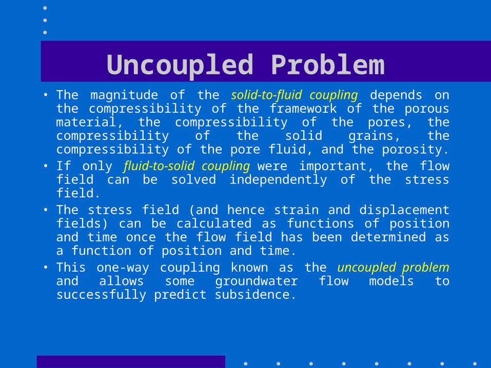
Uncoupled Problem• The magnitude of the solid-to-fluid coupling depends on the

compressibility of the framework of the porous material, the compressibility of the pores, the compressibility of the solid grains, the compressibility of the pore fluid, and the porosity.

• If only fluid-to-solid coupling were important, the flow field can be solved independently of the stress field.

• The stress field (and hence strain and displacement fields) can be calculated as functions of position and time once the flow field has been determined as a function of position and time.

• This one-way coupling known as the uncoupled problem and allows some groundwater flow models to successfully predict subsidence.

Coupled Problem• When the time-dependent changes in stress feed

back significantly to the pore pressure, two-way coupling is important, and is called the coupled problem.

• Applied stress changes in fluid-saturated porous materials typically produce significant changes in pore pressure, and this direction of coupling is significant.

• For this reason, it may be necessary to consider the loading effects of large piles of waste materials in groundwater flow models employed in the mining industry.

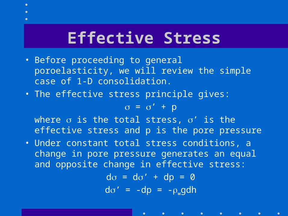
Effective Stress• Before proceeding to general poroelasticity, we will

review the simple case of 1-D consolidation.• The effective stress principle gives:

= ’+ p

where is the total stress, ’ is the effective stress and p is the pore pressure

• Under constant total stress conditions, a change in pore pressure generates an equal and opposite change in effective stress:

d = d’+ dp = 0

d’= -dp = -wgdh

Water Compressibility

• For isothermal compressibility of water:

w = 1/Kw = -(1/Vw)Vw/p

where w is the compressibility of water, Kw is the bulk modulus of compression of water, Vw is the volume of water and p is the pore pressure.

• Mass conservation requires:

wdVw + Vwdw = 0• Using the definition of compressibility:

dVw = -Vwdw/w = -Vw wdp• dVw is the volume change due to compression of

water as a result of a pore pressure increase dp.

Pore Compressibility• The bulk compressibility of a poroelastic material

under one dimensional compression is given by:

b = 1/Kb = -(1/Vb)Vb/’ = -(1/Vp)Vp/’ = p = 1/Hp

where Vb is the bulk volume and Vp is the pore volume. Kb is the bulk modulus of compression and Hp is a vertical bulk modulus of pore compression.

• For incompressible grains: Vb = Vp

• For or a total volume change dVb:

dVb = dVp = -pVbd’ = pVpdp

• dVp is the pore volume change as a result of an effective stress change -d’ = dp

Total Volume Change• The total volume change is:

dVp - dVw = pVbdp + wVwdp

• The water volume Vw = nVb so the volume change is:

dVp - dVw = pVbdp + nwVbdp = Vb(p + nw)dp

• From the expression for total head where z is a constant:

h = z + p/wg or p = wgh - wgz

dp = wgdh

• Note the implicit assumption in this conversion is that w is not a function of pressure.

• Hence: dVp - dVw = Vb(p + nw)wgdh

Total Stress Change

• The effective stress principle for hydrostatic conditions gives:

= ’+ p• Consider an excess pore pressure p as a result of

an applied total stress increment + = ’ + (p + p)

• Flow occurs in order to dissipate the excess pore pressure increment p and over the drainage period the effective stress is increased from ’ to ’ + ’ such that:

+ = ’ + ’ + p

Conservation Statement• In a deforming poroelastic medium there are two conservation

statements. One for fluid mass conservation and one for solid mass conservation. Restricting the discussion to the 1-D case:

• For the fluid mass: -[nwvw]/z = [nw]/t • For the solid mass: -[(1-n)svs]/z = [(1-n)s]/t

where vw and vs are the average velocities with respect to a static frame of reference.

• The Darcy flux is defined relative to the solid matrix so:

qz = n(vw-vs) • Now we introduce a material derivative (not a partial derivative)

that follows the motion of the solid phase (ie any subsidence):

dn/dt = n/t + vs n/z• The total change in porosity with time includes components due

to pore compression within the reference volume and pore displacement with respect to the reference volume.

Grain Incompressibility• Now we assume the grains are incompressible, so s is

constant and all derivatives of s are zero and:• For the solid mass: -s[(1-n)vs]/z = s(1-n)/t

-[(1-n)vs]/z = (1-n)/t

-(1-n)vs/z + vsn/t = -n/t

(1-n)vs/z = n/t + vsn/t

(1-n)vs/z = dn/dt

• For the mass fluid flux, derived from Darcy flux:wqz = nw(vw-vs)

-(wqz)/z = -(nwvw)/z + (nwvs)/z

-(wqz)/z = (nw)/t + vs(nw)/z + nwvs/z

-(wqz)/z - nwvs/z = (nw)/t + vs(nw)/z = d(nw)/dt

-(wqz)/z - nwvs/z = d(nw)/dt

Approximate Conservation Equation• The two derived equations are:

(1-n)vs/z = dn/dt

-(wqz)/z - nwvs/z = d(nw)/dt • From the first equation: vs/z = [1/(1-n)]dn/dt• Substituting in the second equation:

-(wqz)/z - w [n/(1-n)]dn/dt = d(nw)/dt

-(wqz)/z = w[n/(1-n)]dn/dt + wdn/dt + ndw/dt

-(1/w)(wqz)/z = [n/(1-n)]dn/dt + dn/dt + (n/w)dw/dt

-(1/w)(wqz)/z = [1/(1-n)]dn/dt + (n/w)dw/dt• If the volumetric strain of the solid matrix is small, then the total

derivatives can be replaced by the partial derivatives:

-(1/w)(wqz)/z = [1/(1-n)]n/t + (n/w)w/t• Assuming w is independent of z, this reduces to

-qz/z = [1/(1-n)]n/t + (n/w)w/t

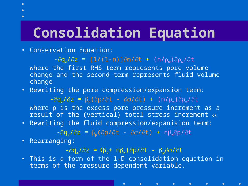
Consolidation Equation• Conservation Equation:

-qz/z = [1/(1-n)]n/t + (n/w)w/twhere the first RHS term represents pore volume change and the second term represents fluid volume change

• Rewriting the pore compression/expansion term:

-qz/z =p(p/t - /t) + (n/w)w/twhere p is the excess pore pressure increment as a result of the (vertical) total stress increment

• Rewriting the fluid compression/expanision term:

-qz/z =p(p/t - /t) + nwp/t• Rearranging:

-qz/z =p+ nw)p/t - p/t• This is a form of the 1-D consolidation equation in terms of the

pressure dependent variable.

Companion Strain Equation• 1-D consolidation equation:

-qz/z =p+ nw)p/t - p/t• Rearranging again:

-qz/z =nwp/t – p(/t - p/t)

-qz/z =nwp/t – p(– p)/t

-qz/z =nwp/t – p’/t• Recognizing the stress-strain relationship for pore

deformation, ’ = /p where is the 1-D (vertical) volumetric strain:

-qz/z =nwp/t – /t• The is the companion equation to the 1-D consolidation

equation written in terms of strain.

More Familiar Forms• 1-D consolidation equation:

-qz/z =p+ nw)p/t - p/t• 1-D companion strain equation:

-qz/z =nwp/t – /t• The equations become more familiar if we recognize:

qz = -Kzh/z = -(Kz/wg)p/z • 1-D consolidation equation:

Kz2p/z2 =wgp+ nw)p/t - wgp/t

Kz2p/z2 =Ssp/t - wgp/t

Kz2h/z2 =Ssh/t - p/t• 1-D companion strain equation:

Kz2p/z2 =n wgwp/t – wg/t

Kz2h/z2 =nwp/t – /t

General Poroelasticity

• A more complete model assumes that all components of the porous medium are compressible, the bulk volume (b), the solid grains (s), the fluids (w), and the pores (p = b - s). 

• The key concepts of Biot’s 1941 poroelastic theory, for an isotropic fluid-filled porous medium, are contained in just two linear constitutive equations, for the case of an isotropic applied stress field .

• In addition to , the other field quantities are the volumetric strain = dV/V, where V is the bulk volume, the increment of fluid content , and the fluid pressure p.

Rice and Cleary

• Rice and Cleary’s 1976 reformulation of Biot’s linear poroelastic constitutive equations has been adopted widely for geophysical problems.

• Rice and Cleary chose constitutive parameters that emphasized the drained (constant pore pressure) and undrained (no flow) limits of long- and short-time behavior, respectively.

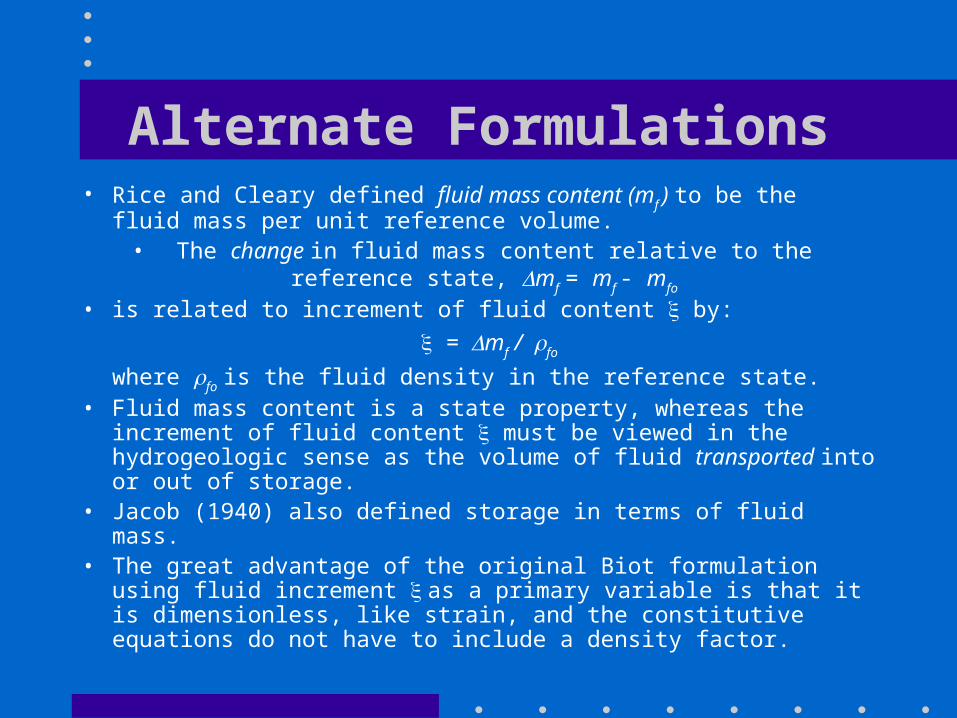
Alternate Formulations• Rice and Cleary defined fluid mass content (mf ) to be the fluid

mass per unit reference volume. • The change in fluid mass content relative to the reference state,

mf = mf - mfo • is related to increment of fluid content by:

=mf /fo

where fo is the fluid density in the reference state. • Fluid mass content is a state property, whereas the increment of

fluid content must be viewed in the hydrogeologic sense as the volume of fluid transported into or out of storage.

• Jacob (1940) also defined storage in terms of fluid mass. • The great advantage of the original Biot formulation using fluid

increment as a primary variable is that it is dimensionless, like strain, and the constitutive equations do not have to include a density factor.

Biot Formulation• The volumetric strain dV/V is taken to be positive in expansion

and negative in contraction. • Stress is positive if tensile and negative if compressive. • Increment of fluid content is positive for fluid added to the

control volume and negative for fluid withdrawn from the control volume.

• Fluid pressure (pore pressure) p greater than atmospheric is positive.

• The constitutive equations simply express and as a linear combination of and p:

= a11 + a12p (1)

= a21 + a22p (2)

• Generic coefficients aij are used in equations (1) and (2) to emphasize the simple form of the constitutive equations.

Linear Equations

• The first constitutive equation is a statement of the observation that changes in applied stress and pore pressure produce a fractional volume change.

• The second constitutive equation is a statement of the observation that changes in applied stress and pore pressure require fluid be added to or removed from storage.

• This second statement implies that applied stress and/or pore pressure might be treated as fluid source terms in groundwater flow equations.

Poroelastic Constants• Poroelastic constants are defined as ratios of field variables

while maintaining various constraints on the elementary control volume.

• The physical meaning of each coefficient in equations (1) and (2) is found by taking the ratio of the change in a dependent variable () relative to the change in an

independent variable (p), while holding the remaining independent variable constant:

• a11 = /|p=0 =1/K = b constant pore pressure

• a12 = /p|=0 =1/H = pconstant total stress

• a21 = /|p=0 = 1/H = p constant pore pressure

• a22 = /p |=0 = 1/R = S = p + nw constant total stress (3)

Drained Compressibilty b

• The coefficient b =1/K is obtained by

measuring the volumetric strain due to changes in applied stress while holding pore pressure constant.

• This state is called a drained condition.

• Therefore, b is the compressibility of the

material measured under drained conditions, and K is the drained bulk modulus.

Poroelastic Expansion Coefficient p

• The coefficient 1/H is a property not encountered in ordinary elasticity.

• It describes how much the bulk volume changes due to a pore pressure change while holding the applied stress constant.

• It is the pore compressibility, that is, the drained bulk compressibility less the grain compression, 1/Hp.

• By analogy with thermal expansion, it is called the poroelastic expansion coefficient.

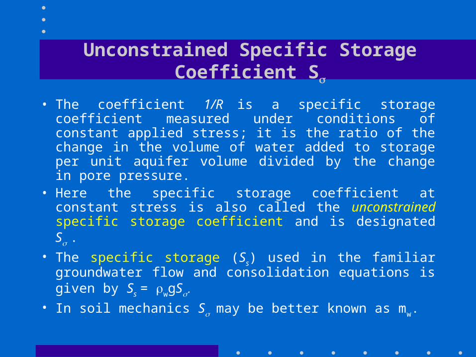
Unconstrained Specific Storage Coefficient S

• The coefficient 1/R is a specific storage coefficient measured under conditions of constant applied stress; it is the ratio of the change in the volume of water added to storage per unit aquifer volume divided by the change in pore pressure.

• Here the specific storage coefficient at constant stress is also called the unconstrained specific storage coefficient and is designated S .

• The specific storage (Ss) used in the familiar groundwater flow and consolidation equations is given by Ss = wgS

• In soil mechanics Smay be better known as mw.

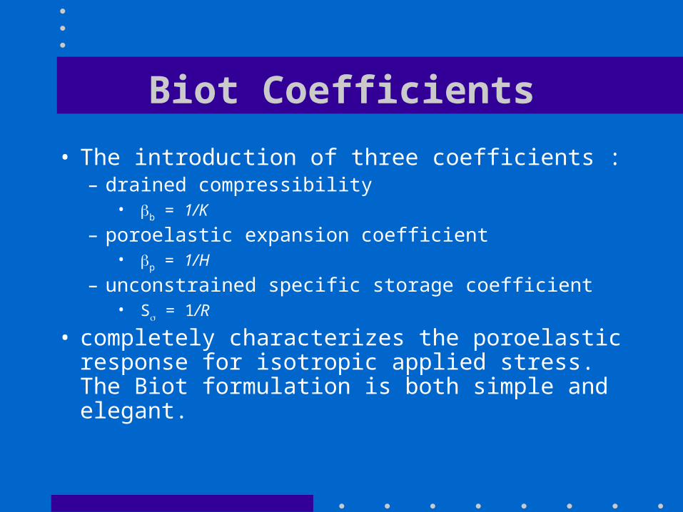
Biot Coefficients

• The introduction of three coefficients :– drained compressibility

• b = 1/K

– poroelastic expansion coefficient • p = 1/H

– unconstrained specific storage coefficient • S = 1/R

• completely characterizes the poroelastic response for isotropic applied stress. The Biot formulation is both simple and elegant.

Coefficient Matrix• These three coefficients are the three independent

components of the symmetric 2 x 2 coefficient matrix relating strain and fluid volume increment to stress and pore pressure.

• Using equation (3) in equations (1) and (2) yields:

 b p p (4)

p Sp (5)

• The drained compressibility (b) and the unconstrained specific storage coefficient (S) are the diagonal components.

• The poroelastic expansion coefficient (p) is the off-diagonal matrix component.

Constrained Specific Storage Coefficient S

• Biot also introduced the coefficient 1/M, which is the specific storage coefficient at constant strain.

• It is called the constrained specific storage coefficient and designated S.

• It is convenient here define the constrained specific storage Se as wgS in an exactly similar manner to Ss.

S = p/|=1/M (6)

Skempton’s Coefficient B

• Skempton’s coefficient (B) is defined to be the ratio of the induced pore pressure to the change in applied stress for undrained conditions - that is, no fluid is allowed to move into or out of the control volume:

B = - p/|=0= R/H = p/S(7)• The negative sign is included in the definition

because the sign convention for stress means that an increase in compressive stress inducing a pore pressure increase implies a decrease in for the undrained condition, when no fluid is exchanged with the control volume.

Meaning of the B Coefficient

• If compressive stress is applied suddenly to a small volume of saturated porous material surrounded by an impermeable boundary, the induced pore pressure is B times the applied stress.

• Skempton’s coefficient must lie between zero and one and is a measure of how the applied stress is distributed between the skeletal framework and the fluid.

• It tends toward one for saturated soils because the fluid supports the load. It tends toward zero for gas-filled pores in soils and for saturated consolidated rocks because the framework supports the load.

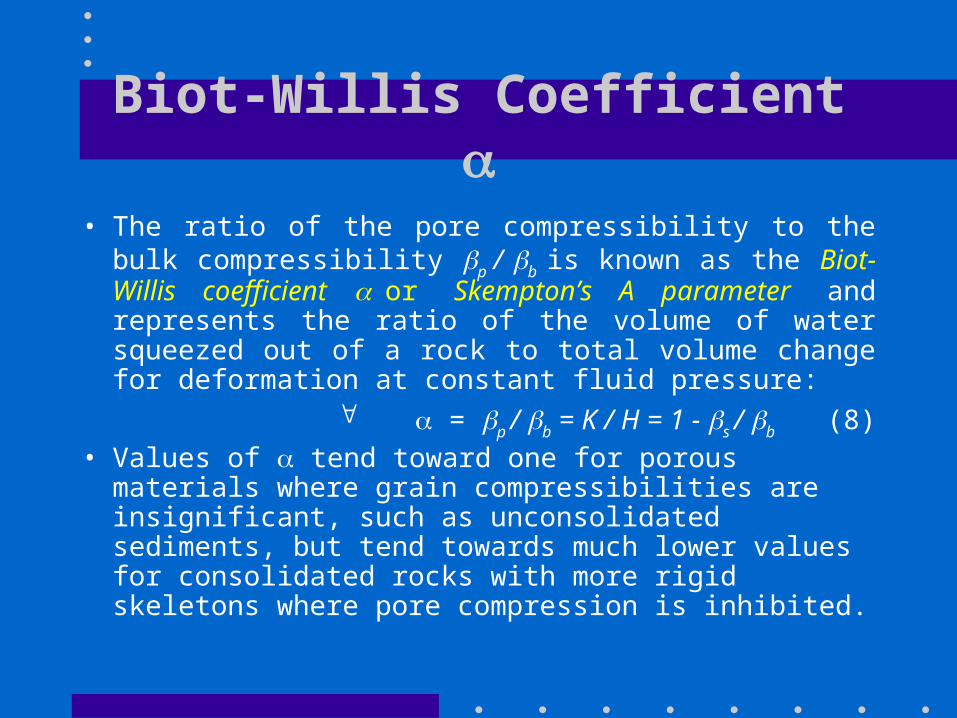
Biot-Willis Coefficient

• The ratio of the pore compressibility to the bulk compressibility p / b is known as the Biot-Willis coefficient or Skempton’s A parameter and represents the ratio of the volume of water squeezed out of a rock to total volume change for deformation at constant fluid pressure:

= p / b = K / H = 1 - s / b (8)• Values of tend toward one for porous materials

where grain compressibilities are insignificant, such as unconsolidated sediments, but tend towards much lower values for consolidated rocks with more rigid skeletons where pore compression is inhibited.

Specific Storage Coefficients

• The (constrained) specific storage coefficient at constant strain (S) is smaller than the (unconstrained) specific storage coefficient at constant stress (S) due to the constraint that the bulk volume remains constant.

• Algebraic manipulation shows that:

S = S + p (9)

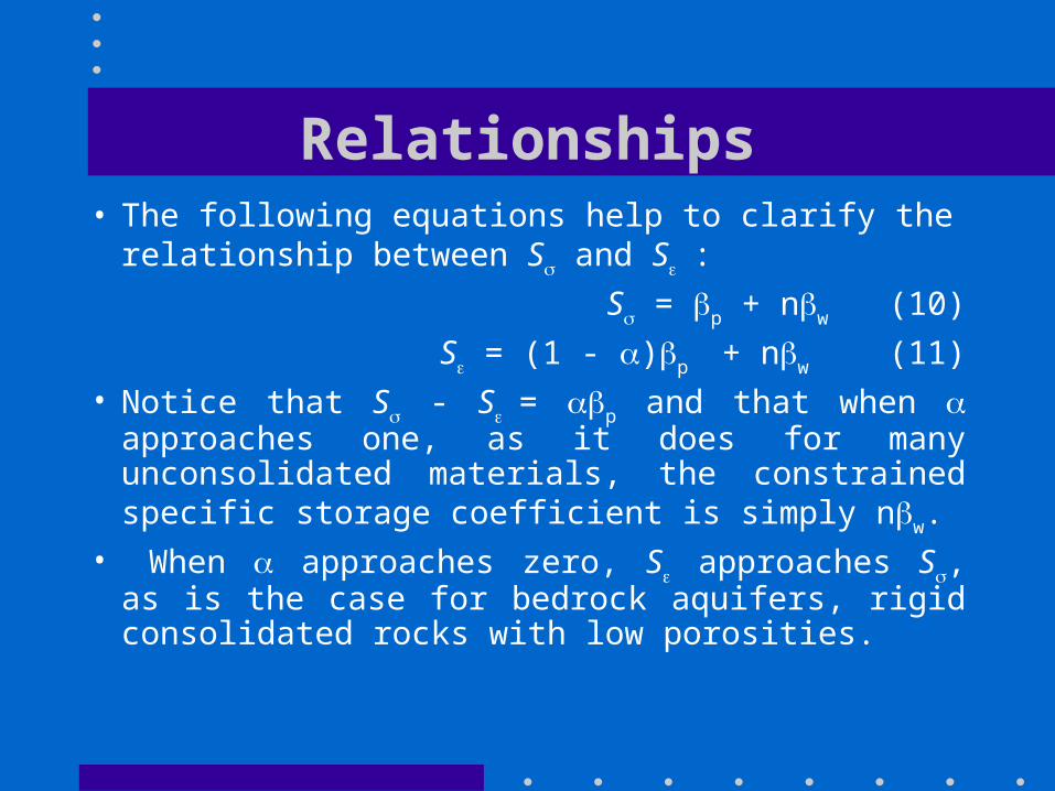
Relationships• The following equations help to clarify the relationship

between S and S:

S = p + nw (10)

S = (1 - )p + nw (11)

• Notice that S - S= p and that when approaches one, as it does for many unconsolidated materials, the constrained specific storage coefficient is simply nw.

• When approaches zero, S approaches S, as is the case for bedrock aquifers, rigid consolidated rocks with low porosities.

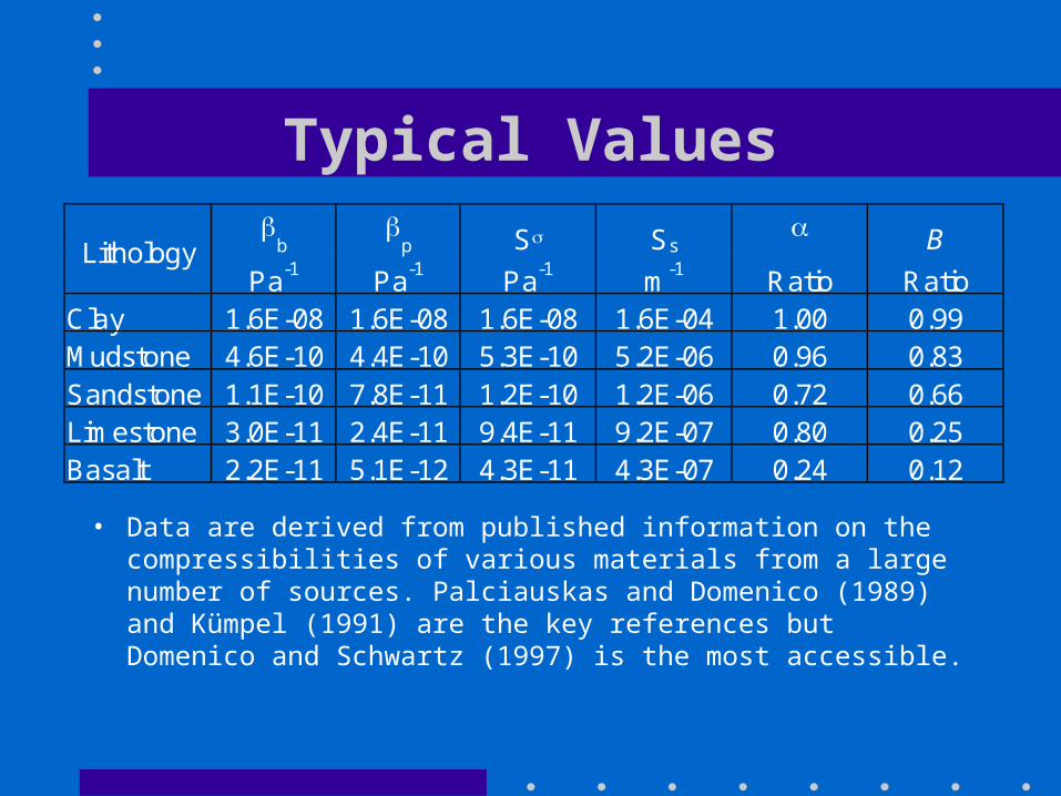
Typical Values

• Data are derived from published information on the compressibilities of various materials from a large number of sources. Palciauskas and Domenico (1989) and Kümpel (1991) are the key references but Domenico and Schwartz (1997) is the most accessible.

b

p S Ss B Lithology Pa-1 Pa-1 Pa-1 m-1 Ratio Ratio

Clay 1.6E-08 1.6E-08 1.6E-08 1.6E-04 1.00 0.99 Mudstone 4.6E-10 4.4E-10 5.3E-10 5.2E-06 0.96 0.83 Sandstone 1.1E-10 7.8E-11 1.2E-10 1.2E-06 0.72 0.66 Limestone 3.0E-11 2.4E-11 9.4E-11 9.2E-07 0.80 0.25 Basalt 2.2E-11 5.1E-12 4.3E-11 4.3E-07 0.24 0.12

Flow Equations• Palciauskas and Domenico (1989) presented the flow equations

for completely deformable porous media. • Equation (12) incorporates stress changes over time (the

second RHS term) as a mechanism to generate excess pore pressures:

  p = [ K p] + B (12)

t Ss t• The companion equation (13) incorporates pore volume strain

(the second RHS term) as a mechanism to generate excess pore pressures: 

p = [ K p] + (13)

t Se St

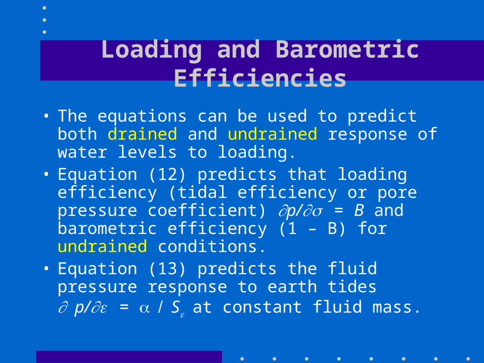
Loading and Barometric Efficiencies

• The equations can be used to predict both drained and undrained response of water levels to loading.

• Equation (12) predicts that loading efficiency (tidal efficiency or pore pressure coefficient) p/ = B and barometric efficiency (1 – B) for undrained conditions.

• Equation (13) predicts the fluid pressure response to earth tides p/ = Sat constant fluid mass.

Tidal Fluctuations

Earth Tides

Barometric Response

1-D Consolidation Theory

• Biot showed at an early stage that Terzaghi’s one-dimensional consolidation problem is a special case of his theory. One-dimensional consolidation theory (Terzhagi consolidation) assumes:

• (1)   the stress increment generating the excess fluid pressure is vertical and

• (2) the solid components of the rock/soil matrix are incompressible. • The first assumption is implicit in the three-dimensional forms given

in equations (12) and (13) since no shear stress-strain components are included.

• The second assumption means that bulk volume changes are exactly equal to pore volume changes, that is, is one. These are reasonable approximations for many practical purposes but neither assumption is strictly true.

Modelling Subsidence• Most of the calculations used to estimate subsidence are

based on Terzaghi’s simple one-dimensional analytical model (Poland and Davis, 1969). Terzaghi’s principle of effective stress coupled with Hubbert’s force potential and Darcy’s Law provided the basis for one-dimensional subsidence modelling (Gambolati et al, 1974).

p = [ K p] + Q (14)

t Ss • When the change in mean total stress is assumed to be

negligible within a ground-water basin, equation (12) reduces to equation (14) and becomes identical to the traditional groundwater flow equation used in many models.

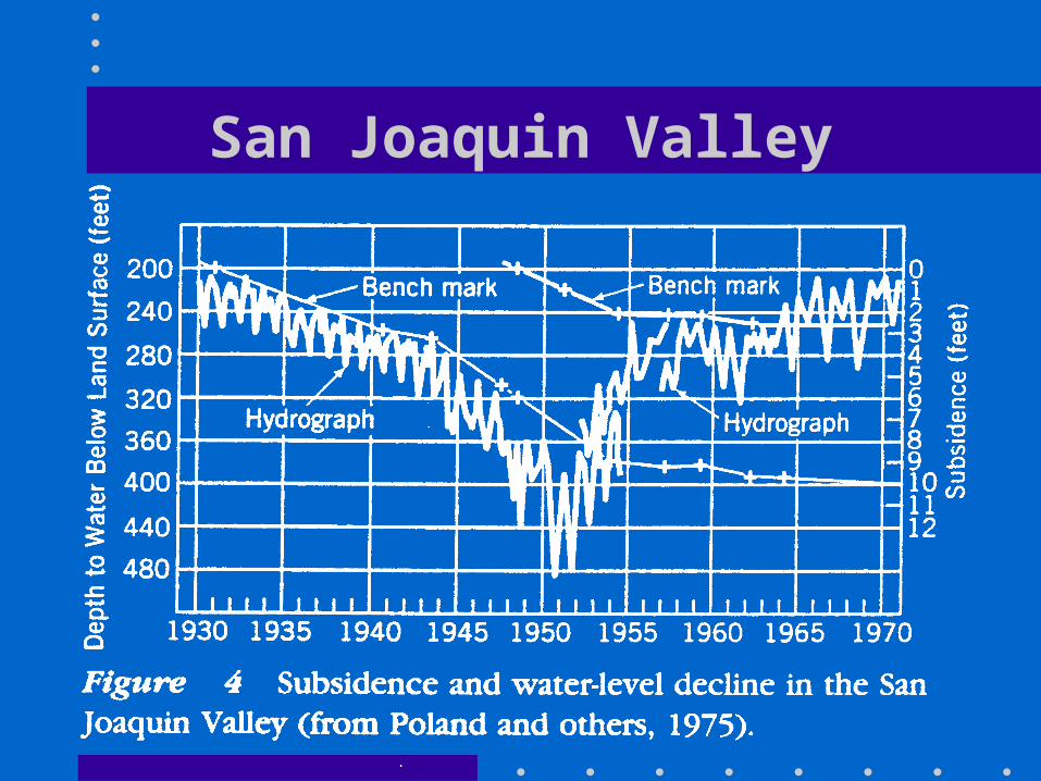
San Joaquin Valley

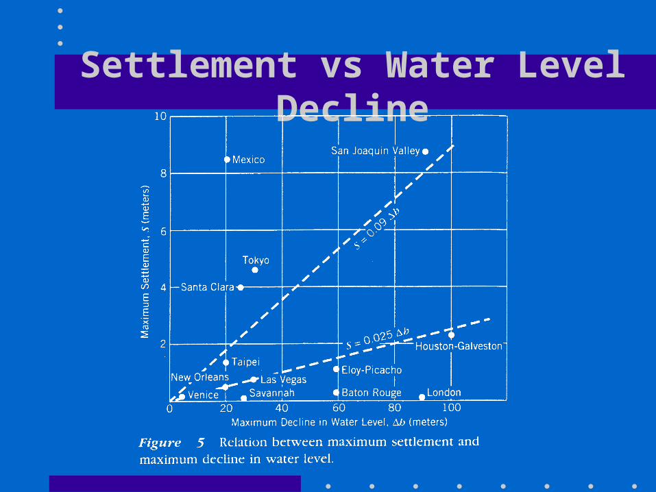
Settlement vs Water Level Decline

Terzhagi’s Equation

• For the one-dimensional case writing Cv = K/Ss ,

reveals Terzhagi’s familiar consolidation equation: 

p = K p = K p = Cv p (15)

t Ss z2 mwwg z2 z2

• This is perhaps the most famous equation incorporating poroelastic effects but it conceals a very large number of assumptions and simplifications which make it inappropriate as a starting point for a more rigorous analysis.

Las Vegas Subsidence Profile

Modelling Total Stress Changes

• Most numerical models used to simulate groundwater flow (equation 14) were derived with the assumption that the total stress imposed on the aquifer remains constant with time.

• If the aquifer is subjected to time-varying total stresses (loading), these models are inappropriate.

• In such cases, a more general model that accounts for aquifer deformation is required.

• The effect of changes in total stress on an aquifer system has been considered by many authors for a variety of applications.

Total Stress Change Examples• Gibson (1958) discusses the impact of increasing clay thickness

on the consolidation of a clay unit and introduces a source term to the equation describing the excess pore-water pressure increment associated with the loading.

• Abnormal pressure, both over-pressure and under-pressure, in both aquifers and oil reservoirs, has been studied by Bredehoeft and Hanshaw (1968), Neuzil (1993), and Neuzil (1995).

• For these systems, changes in the total stress applied to the system occur as a result of the slow geologic processes of sedimentation or erosion.

• Provost et al. (1998) considered the preconsolidation pressures induced by changes in total stress due to glaciation in a long-term model for a proposed nuclear waste repository.

• Gardner et al. (1998) found that inclusion of pore pressures derived from tidal loading of peat in salt marshes was necessary in order to match observed piezometric responses.

Rate of Pore Pressure Dissipation

• Equation (15) is readily solved for constant head conditions (Terzhagi, 1943) and an analytical expression can be derived to predict the time needed for dissipation of a specified percentage of any increment of excess pore-pressure by vertical drainage:

tp = d2SsTv = d2Tv (16)

K Cv

where tp is the time, d is the drainage distance, and Tv is

consolidation time factor.

Vertical and Radial Drainage

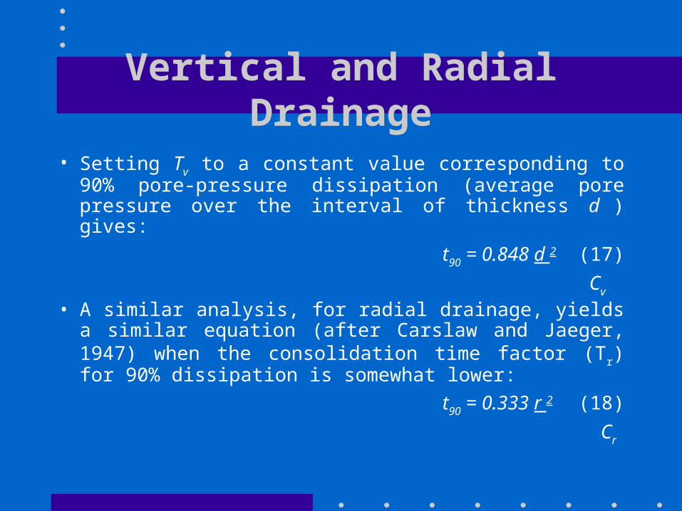
• Setting Tv to a constant value corresponding to 90% pore-pressure dissipation (average pore pressure over the interval of thickness d ) gives:

t90 = 0.848 d 2 (17)

Cv  • A similar analysis, for radial drainage, yields a similar

equation (after Carslaw and Jaeger, 1947) when the consolidation time factor (Tr) for 90% dissipation is somewhat lower:

t90 = 0.333 r 2 (18)

Cr

Constant Loading Rate

• Abashi (1970) derived an addition useful analytic solution for the vertical consolidation equation with a constant rate of monotonic loading (rather than a constant instantaneous load). The time factor Tc for 90% dissipation is larger than for the instantaneous load case:

t90 = 0.946 d 2 (19)

Cv

• The constant loading rate solution is not used as commonly at the Terzhagi solution in practice, but is valuable for the analysis of embankment construction and pile building.