Unimodular Random Triangulations: Circle Packing …...Unimodular Random Triangulations: Circle...
38
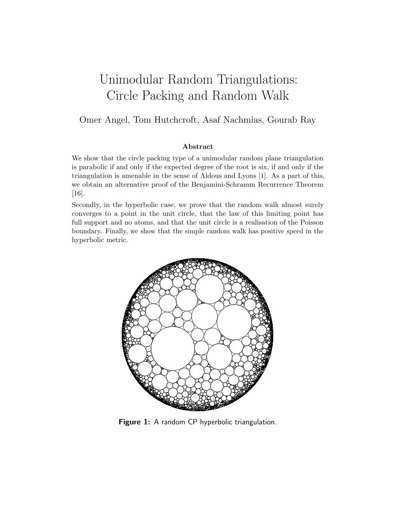
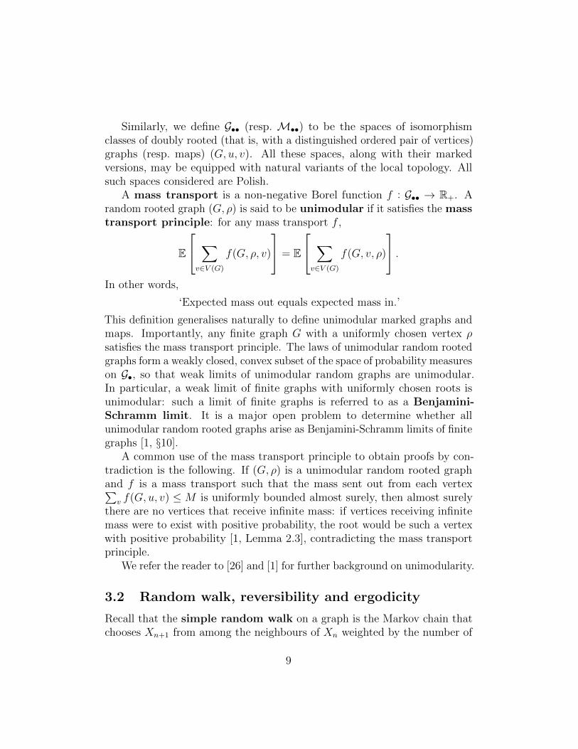
Unimodular Random Triangulations: Circle Packing and Random Walk Omer Angel, Tom Hutchcroft, Asaf Nachmias, Gourab Ray Abstract We show that the circle packing type of a unimodular random plane triangulation is parabolic if and only if the expected degree of the root is six, if and only if the triangulation is amenable in the sense of Aldous and Lyons [1]. As a part of this, we obtain an alternative proof of the Benjamini-Schramm Recurrence Theorem [16]. Secondly, in the hyperbolic case, we prove that the random walk almost surely converges to a point in the unit circle, that the law of this limiting point has full support and no atoms, and that the unit circle is a realisation of the Poisson boundary. Finally, we show that the simple random walk has positive speed in the hyperbolic metric. Figure 1: A random CP hyperbolic triangulation.
Transcript of Unimodular Random Triangulations: Circle Packing …...Unimodular Random Triangulations: Circle...
Unimodular Random Triangulations:Circle Packing and Random Walk
Omer Angel, Tom Hutchcroft, Asaf Nachmias, Gourab Ray
Abstract
We show that the circle packing type of a unimodular random plane triangulationis parabolic if and only if the expected degree of the root is six, if and only if thetriangulation is amenable in the sense of Aldous and Lyons [1]. As a part of this,we obtain an alternative proof of the Benjamini-Schramm Recurrence Theorem[16].
Secondly, in the hyperbolic case, we prove that the random walk almost surelyconverges to a point in the unit circle, that the law of this limiting point hasfull support and no atoms, and that the unit circle is a realisation of the Poissonboundary. Finally, we show that the simple random walk has positive speed in thehyperbolic metric.
Figure 1: A random CP hyperbolic triangulation.
1 Introduction
A circle packing of a planar graph G is a set of circles with disjoint interiorsin the plane, one for each vertex of G, such that two circles are tangent if andonly if their corresponding vertices are adjacent in G. The Koebe-Andreev-Thurston Circle Packing Theorem [24, 33] states that every finite simpleplanar graph has a circle packing; if the graph is a triangulation, the packingis unique up to Mobius transformations and reflections. He and Schramm [22]extended this theorem to infinite, one-ended, simple triangulations, showingthat each such triangulation admits either a locally finite circle packing inthe Euclidean plane or in the hyperbolic plane (identified with the interiorof the unit disc), but not both. See Section 3.4 for precise details. This isa discrete analogue of the Uniformization Theorem, which states that everysimply connected, non-compact Riemann surface is conformally equivalent toeither the plane or the disc (in fact, there are deep connections between circlepacking and conformal maps, see [30, 32] and references therein). Accordingly,a triangulation is called CP parabolic if it may be circle packed in the planeand CP hyperbolic otherwise.
Circle packing has proven instrumental in the study of random walks onplanar graphs [13, 16, 22, 20]. In the case of graphs with bounded degrees, arich theory has been established connecting the geometry of the circle packingand the behaviour of the random walk. Most notably, a one-ended, boundeddegree triangulation is CP hyperbolic if and only if random walk on it istransient [22] and in this case it is also non-Liouville, i.e. admits non-constantbounded harmonic functions [13].
The goal of this work is to develop a similar, parallel theory for randomtriangulations. Particular motivations come from the Markovian hyperbolictriangulations constructed recently in [8] and [17]. These are hyperbolicvariants of the UIPT [9] and are conjectured to be the local limits of uniformtriangulations in high genus. Another example is the Poisson-Delaunaytriangulation in the hyperbolic plane, studied in [15] and [12]. Unfortunately,these triangulations have unbounded degrees, rendering existing methods (forexample those of [3, 13, 22]) ineffective.
Indeed, in the absence of bounded degree the existing theory fails in manyways. In this paper we wish to examine circle packings of unbounded degree,yet the resulting absence of a uniform bound on the ratios of the radii ofadjacent circles invalidates many important resistance estimates. This is nota mere technicality: one can add extra circles in the interstices of the circle
2

packing of the triangular lattice to create drifts in arbitrary directions. Thisdoes not change the circle packing type, but allows construction of a graphthat is CP parabolic but transient or even non-Liouville. Indeed, the maineffort in [20] was to overcome this sole obstacle in order to prove that theUIPT is recurrent.
The hyperbolic random triangulations of [17] and [12] make up for havingunbounded degrees by a different useful property: unimodularity (essen-tially equivalent to reversibility, see Sections 3.1 and 3.2). This allows usto apply probabilistic and ergodic arguments in place of the analytic ar-guments appropriate to the bounded degree case. Our first main theoremestablishes a probabilistic characterisation of the CP type for unimodularrandom rooted triangulations. The relevant probabilistic property is invariant(non-)amenability, which we define in Section 3.3.
Theorem 1.1. Let (G, ρ) be an infinite, unimodular, ergodic, one-ended andsimple planar triangulation and suppose E[deg(ρ)] <∞. Then either
E[deg(ρ)] = 6, in which case (G, ρ) is invariantly amenable andalmost surely CP parabolic,
or
E[deg(ρ)] > 6, in which case (G, ρ) is invariantly non-amenableand almost surely CP hyperbolic.
This theorem can be viewed as a local-to-global principle for unimodulartriangulations. That is, it allows us to identify the CP type and invariantamenability, global properties, by calculating the expected degree, a verylocal quantity. For example, if (G, ρ) is a simple, one-ended triangulationthat is obtained as a local limit of planar graphs, then by Euler’s formulaand Fatou’s lemma its average degree is at most 6, so that Theorem 1.1implies it is CP parabolic. If in addition (G, ρ) has bounded degrees, then itis recurrent almost surely by He-Schramm [22]. In particular, this gives analternative proof of the Benjamini-Schramm Theorem [16] in the relevant andmost significant case of a one-ended limit (in section 4.1 we show that theremaining cases follow easily from well-known arguments). Unlike the proof of[16], whose main ingredient is a quantitative estimate for finite circle packings[16, Lemma 2.3], our method works with infinite triangulations directly andimplies the following generalisation:
3
Proposition 1.2. Any unimodular, simple, one-ended random rooted planartriangulation (G, ρ) with bounded degrees and E[deg(ρ)] = 6 is almost surelyrecurrent.
In a future paper, however, we show that any graph to which this resultapplies is also a local limit of finite planar graphs with bounded degrees,and consequently there are no graphs to which this result applies and theBenjamini-Schramm Theorem does not. We remark that the dichotomy ofTheorem 1.1 has many extensions, applying to more general maps and holdingfurther properties equivalent. We address these in future work [6].
Our method of proof relies on the deep theorem of Schramm [31] thatthe circle packing of a triangulation in the disc or the plane is unique upto Mobius transformations fixing the disc or the plane as appropriate. Weuse this fact throughout the paper in an essential way: it implies that anyquantity of the circle packing in the disc or the plane that is invariant toMobius transformations (most importantly, angles between adjacent edges inthe associated drawings with hyperbolic or Euclidean geodesics, see Section 4)are in fact determined by the graph G and not by our choice of circle packing.
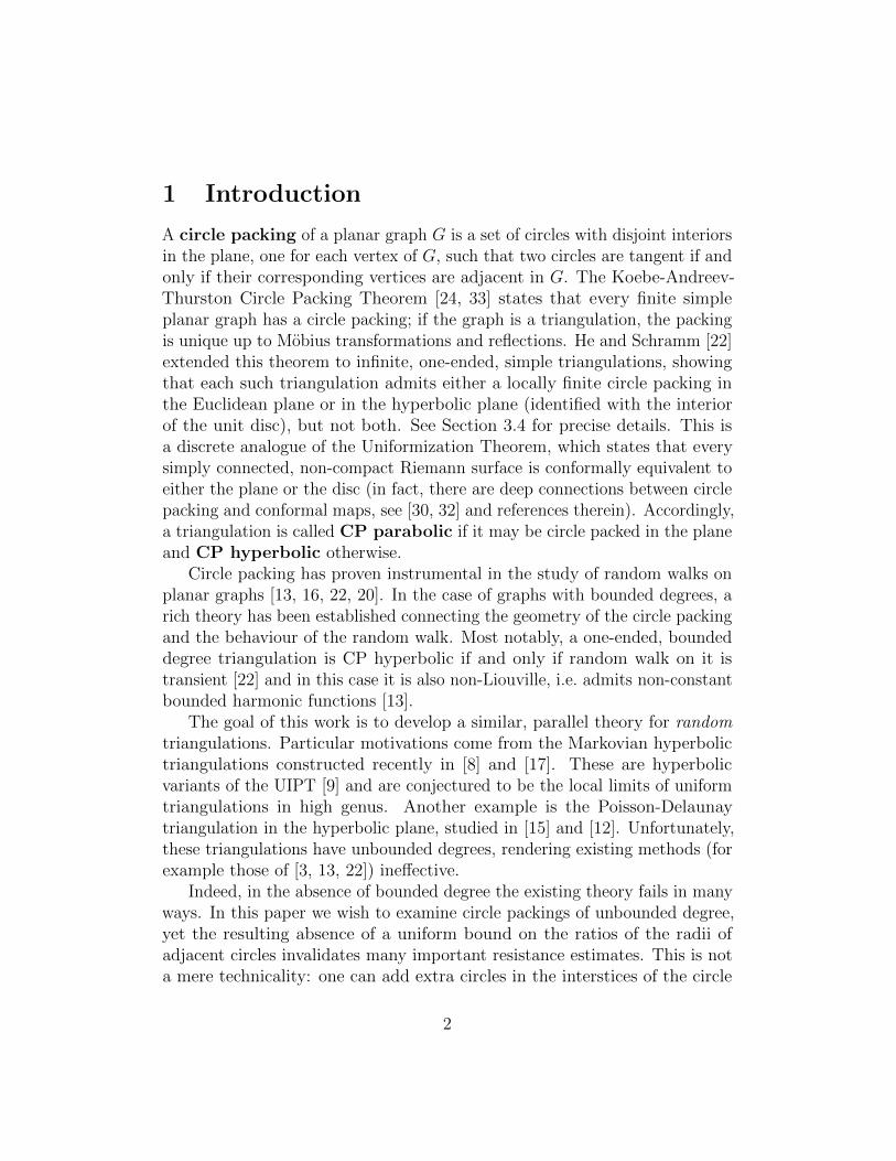
Boundary Theory. In the CP hyperbolic case, the circle packing in thehyperbolic plane realised as the unit disc gives rise to a natural geometricboundary for G (namely, the unit circle). When G has bounded degreesthis geometric boundary is known to coincide with probabilistic notions ofthe boundary. Benjamini and Schramm [13] showed that the random walkconverges to a point in the circle almost surely and that the law of the limitpoint has full support and is non-atomic. More recently, it was shown by thefirst and third authors with Barlow and Gurel-Gurevich [3] that the unit circleis a realisation of both the Poisson and Martin boundaries of the triangulation.Similar results regarding square tiling were obtained in [14] and [19].
Again, these theorems fail for some graphs with unbounded degrees. Wecan impose a drift along chosen paths in a graph, forcing the random walk tospiral in the disc and not converge to any point in the boundary, or allowingit to converge to a single boundary point from two or more different angleseach with positive probability (so that the exit measure is atomic and theunit circle is no longer a realisation of the Poisson boundary). The next resultrecovers the boundary theory in the unimodular setting.
When C is a circle packing of a graph G in the disc D, we write C = (z, r)where z(v) is the (Euclidean) centre of the circle corresponding to v, and r(v)
4

its Euclidean radius. We also write zh(v) for the hyperbolic centres of thecircles. Recall that the hyperbolic metric on the unit disc is defined by
|dhyp(z)| = |dz|1− |z|2
,
and that circles in the Euclidean metric are also hyperbolic circles (withdifferent centres and radii). We use PG
v and EGv to denote the probability
and expectation with respect to random walk (Xn)n≥0 on G started from avertex v.
Theorem 1.3. Let (G, ρ) be a simple, one-ended, CP hyperbolic unimodularrandom planar triangulation with E[deg2(ρ)] <∞ and let C be a circle packingof G in the unit disc. The following hold conditional on (G, ρ) almost surely:
1. z(Xn) and zh(Xn) both converge to a point z(X∞) ∈ ∂D,
2. The law of z(X∞) has support ∂D and no atoms.
3. ∂D is a realisation of the Poisson boundary of G. That is, for everybounded harmonic function h on G there exists a bounded measurablefunction g : ∂D→ R such that
h(v) = EGv [g(z(X∞))].
We refer to the law of z(X∞) conditional on (G, ρ) as the exit measure.Our final result relates exponential decay of the Euclidean radii along therandom walk to speed in the hyperbolic metric.
Theorem 1.4. Let (G, ρ) be a simple, one-ended, CP hyperbolic unimodularrandom rooted planar triangulation with E[deg2(ρ)] <∞ and let C be a circlepacking of G in the unit disc. Then
limn→∞
dhyp(zh(ρ), zh(Xn))
n= lim
n→∞
− log r(Xn)
n> 0
almost surely. That is, the random walk (Xn) has positive hyperbolic speedand the Euclidean radii along the walk decay exponentially. If (G, ρ) is ergodicthen this limit is an almost sure constant and does not depend on the choiceof packing.
5

Organization of the paper. In Section 2 we give examples of unimodularhyperbolic random triangulations to which our results apply. In Section 3.1and Section 3.2 we give background on unimodularity, reversibility andrelated topics. In Section 3.3 we recall Aldous and Lyons’s notion of invariantamenability and give a proof of one of its important properties. In Section 3.4we recall the required results on circle packing and discuss measurability.Section 4 contains the proof of Theorem 1.1 as well as a discussion of how tohandle the remaining cases of the Benjamini-Schramm Theorem. Theorem 1.3is proven in Section 5 and Theorem 1.4 is proven in Section 6. Background onthe Poisson boundary is provided before the proof of item 3 of Theorem 1.3in Section 5.3. In Section 7 we discuss extensions of our results to non-simpleand weighted triangulations. We end with some open problems in Section 8.
2 Examples
Benjamini-Schramm limits of random maps have been objects of great interestin recent years, serving as discrete models of 2-dimensional quantum gravity.Roughly, the idea is to consider a class of random rooted maps (e.g. allpossible triangulations or quadrangulations of the sphere of size n) and takea local limit as the size of the maps become large [9, 2, 10, 18, 5, 4].
Curien’s PSHT. Recently, hyperbolic versions of such maps have beenconstructed: half-plane versions in [8] and full-plane versions in [17]. The fullplane triangulations form a one (continuous) parameter family Tκκ∈(0,2/27)
(known as the PSHT: Planar Stochastic Hyperbolic Triangulation) and arereversible and ergodic. They are known to have anchored expansion andare therefore invariantly non-amenable. They are also known to have anexponential tail on the degree at the root, so that in particular the firstmoment is finite.
Although these triangulations are not simple, we are still able to obtain ageometric representation of their Poisson boundary by circle packing theirsimple cores, see Section 7.
Benjamini-Schramm limits of maps in high genus. It is conjecturedthat the PSHT Tκ arises as a Benjamini-Schramm limit of the uniformtriangulation with n vertices of the bθ(κ)nc-holed torus for some θ(κ) (see[28] for precise definitions of maps on general surfaces), and we expect thatother interesting one-ended unimodular random rooted planar triangulations
6

may be constructed as Benjamini-Schramm limits of finite triangulationswhose genus is linear in their size.
In the context of circle packing, it may be particularly interesting to takethe Benjamini-Schramm limit (T, ρ) of the uniform simple triangulation withn vertices of the bθnc-holed torus Tn. This limit (which we do not knowexists) should be a simple variant of the PSHT. Letting ρn be a uniformlychosen root of Tn, it should also be the case that E[deg(ρn)]→ E[deg(ρ)] > 6and E[deg(ρ)2] < ∞, so that our results would be applicable to the circlepacking of (T, ρ).
Delaunay triangulations of the hyperbolic plane. Suppose we take aPoisson point process in the hyperbolic plane with intensity given by a multipleof the area measure, and add a point at the origin. This point process generatesa triangulation of the hyperbolic plane, called the Delaunay triangulation,whose vertices are given by the points of the process and whose edges aredrawn with geodesics. These triangulations, studied in [15] and [12], areknown to be unimodular when rooted at the point at the origin and haveanchored expansion [12], so are invariantly non-amenable. (Alternatively,one can show their expected degree to be greater than six by transportingangles as in the proof of Theorem 1.1, obtaining invariant non-amenability asa consequence of that theorem.) They are also simple and one-ended almostsurely and the degree of the root has finite second moment, so that our resultsapply directly to their circle packings.
We expect that our methods should also extend without too much difficultyto derive similar results for the embedding that the Delaunay triangulationbegins with. In particular, if one can show that the random walk converges toa point in the boundary of the hyperbolic plane and that the law of the limitpoint is non-atomic almost surely, our proof immediately generalises to provethat the hyperbolic boundary is a realisation of the Poisson boundary. Similarremarks apply to other kinds of geometric embeddings of planar maps intothe hyperbolic plane, such as the embedding arising from the UniformizationTheorem.
7

3 Background and Definitions
3.1 Unimodular random graphs and maps
A rooted graph (G, ρ) is a graph G = (V,E) with a distinguished vertex ρcalled the root. We will allow our graphs to contain self-loops and multipleedges, and refer to graphs without either as simple. A graph is called one-ended if the removal of any finite set of vertices leaves precisely one infiniteconnected component. A graph isomorphism between two rooted graphs is arooted graph isomomorphism if it preserves the root.
A planar map is a proper (that is, with non-intersecting edges) embeddingof a graph into a surface (in this paper, the sphere, the plane or the disc) viewedup to orientation preserving homeomorphisms of the surface. Connectedcomponents of the complement of the embedding are called faces. A map isa triangulation if every face is incident to exactly three edges.
Every connected graph can be made into a metric space by endowingit with the shortest path metric dG. By abuse of notation, we use the ballBn(G, u) to refer both to the set of vertices v ∈ V : dG(u, v) ≤ n and theinduced subgraph on this set, rooted at u. The balls in a map inherit a mapstructure from the full map.
The local topology on isomorphism classes of rooted graphs (introducedin [16]) is the topology induced by the metric
d((G, ρ), (G′, ρ′)) = e−R where R = supn ≥ 0 : Bn(G, ρ) ∼= Bn(G′, ρ′).
The local topology on isomorphism classes of rooted maps is defined similarlyby requiring the isomorphism of the balls to be an isomorphism of rootedmaps. We denote by G• and M• the spaces of isomorphism classes of rootedgraphs and maps with their respective local topologies; random rootedgraphs and maps are Borel random variables taking values in these spaces.
Several variants of these spaces will also be important. A (countably)marked graph is a graph together with a marking m : V ∪ E → M whichgives every edge and vertex a mark in some countable set M . A graph isomo-morphism between marked graphs is an isomomorphism of marked graphsif it preserves the marks, and we define the local topologies on isomorphismclasses of rooted marked graphs and rooted marked maps in the obvious way,denoting these spaces GM• andMM
• . Marked graphs are special cases of whatAldous and Lyons [1] call networks, for which the marks may take values inany separable complete metric space.
8
Similarly, we define G•• (resp. M••) to be the spaces of isomorphismclasses of doubly rooted (that is, with a distinguished ordered pair of vertices)graphs (resp. maps) (G, u, v). All these spaces, along with their markedversions, may be equipped with natural variants of the local topology. Allsuch spaces considered are Polish.
A mass transport is a non-negative Borel function f : G•• → R+. Arandom rooted graph (G, ρ) is said to be unimodular if it satisfies the masstransport principle: for any mass transport f ,
E
∑v∈V (G)
f(G, ρ, v)
= E
∑v∈V (G)
f(G, v, ρ)
.In other words,
‘Expected mass out equals expected mass in.’
This definition generalises naturally to define unimodular marked graphs andmaps. Importantly, any finite graph G with a uniformly chosen vertex ρsatisfies the mass transport principle. The laws of unimodular random rootedgraphs form a weakly closed, convex subset of the space of probability measureson G•, so that weak limits of unimodular random graphs are unimodular.In particular, a weak limit of finite graphs with uniformly chosen roots isunimodular: such a limit of finite graphs is referred to as a Benjamini-Schramm limit. It is a major open problem to determine whether allunimodular random rooted graphs arise as Benjamini-Schramm limits of finitegraphs [1, §10].
A common use of the mass transport principle to obtain proofs by con-tradiction is the following. If (G, ρ) is a unimodular random rooted graphand f is a mass transport such that the mass sent out from each vertex∑
v f(G, u, v) ≤ M is uniformly bounded almost surely, then almost surelythere are no vertices that receive infinite mass: if vertices receiving infinitemass were to exist with positive probability, the root would be such a vertexwith positive probability [1, Lemma 2.3], contradicting the mass transportprinciple.
We refer the reader to [26] and [1] for further background on unimodularity.
3.2 Random walk, reversibility and ergodicity
Recall that the simple random walk on a graph is the Markov chain thatchooses Xn+1 from among the neighbours of Xn weighted by the number of
9

shared edges. Define G↔ (resp. M↔) to be spaces of isomorphism classesof graphs (resp. maps) equipped with a bi-infinite path (G, (xn)n∈Z), whichwe endow with a natural variant of the local topology. When (G, ρ) is arandom graph or map, we let (Xn)n≥0 and (X−n)n≥0 be two independentsimple random walks started from ρ and consider (G, (Xn)n∈Z) to be a randomelement of G↔ or M↔ as appropriate.
A random rooted graph (G, ρ) is stationary if (G, ρ)d= (G,X1) and
reversible if (G, ρ,X1)d= (G,X1, ρ) as doubly rooted graphs. Equivalently,
(G, ρ) is reversible if and only if (G, (Xn)n∈Z) is stationary with respect tothe shift:
(G, (Xn)n∈Z)d= (G, (Xn+k)n∈Z) for every k ∈ Z.
To see this, it suffices to prove that if (G, ρ) is a reversible random graphthen (X1, ρ,X−1, X−2, . . .) has the law of a simple random walk started fromX1. But (ρ,X−1, . . .) is a simple random walk started from ρ independentof X1 and, conditional on (G,X1), reversibility implies that ρ is uniformlydistributed among the neighbours of X1, so (X1, ρ,X−1, X−2, . . .) has the lawof a simple random walk as desired.
We remark that if (G, ρ) is stationary but not necessarily reversible, it isstill possible to extend the walk to a doubly infinite path (Xn)n∈Z so that Gis stationary along the path. The difference is that in the reversible case thepast (Xn)n≤0 is itself a simple random walk, independent of the future.
Reversibility is related to unimodularity via the following bijection: if(G, ρ) is reversible, then biasing by deg(ρ)−1 (i.e. reweighting the law of (G, ρ)by the Radon-Nikodym derivative deg(ρ)−1/E[deg(ρ)−1]) gives an equivalentunimodular random network, and conversely if (G, ρ) is a unimodular randomnetwork with finite expected degree, then biasing by deg(ρ) gives an equivalentreversible random network (see [1, Theorem 4.1]).
An event A ⊂ G↔ is said to be invariant if (G, (Xn)n∈Z) ∈ A implies(G, (Xn+k)n∈Z) ∈ A for each k ∈ Z. A reversible random graph is said tobe ergodic if the law of (G, (Xn)n∈Z) gives each invariant event probabilityeither zero or one.
Theorem 3.1 (Characterisation of ergodicity [1, §4]). Let (G, ρ) be a re-versible random rooted graph. The following are equivalent.
1. (G, ρ) is ergodic.
2. Every event A ⊂ G• invariant to changing the root has probability in0, 1.
10

3. The law of (G, ρ) is an extreme point of the weakly closed convex set oflaws of reversible random rooted graphs.
A consequence of the extremal characterisation is that every reversiblerandom rooted graph is a mixture of ergodic reversible random rooted graphs,meaning that it may be sampled by first sampling a random law of an ergodicreversible random rooted graph, and then sampling from this randomlychosen law - this is known as an ergodic decomposition and its existence is aconsequence of Choquet’s Theorem.
In particular, whenever we want to prove that a reversible random rootedgraph with some almost sure property also has some other almost sureproperty, it suffices to consider the ergodic case.
3.3 Invariant amenability
We begin with a brief review of general amenability, before combining it withunimodularity for the notion of invariant amenability. We refer the reader to[26, §6] for further details on amenability in general, and [1, §8] for invariantamenability.
A weighted graph is a graph together with a weight function w : E → R+.Unweighted multigraphs may always be considered as weighted graphs byhaving w ≡ 1. A weight function is extended to vertices by w(x) =
∑e3xw(e),
and (with a slight abuse of notation) to sets of edges or vertices by additivity.The simple random walk X = (Xn)n≥0 on a weighted graph is the Markovchain on V with transition probabilities p(x, y) = w(x, y)/w(x). Here, ourgraphs are allowed to have infinite degree provided w(v) is finite for everyvertex.
The (edge) Cheeger constant of an infinite weighted graph is definedto be
iE(G) = inf
w(∂EW )
w(W ): W ⊂ V finite
where ∂EW denotes the set of edges with exactly one end in W . A graph issaid to be amenable if its Cheeger constant is zero and non-amenable if itis positive.
The Markov operator associated to simple random walk on G is thebounded, self-adjoint operator from L2(V,w) to itself defined by (Pf)(u) =∑p(u, v)f(v). The norm of this operator is commonly known as the spectral
11

radius of the graph. If u, v ∈ V then the transition probabilities are givenby pn(u, v) =
⟨P n
1v,1u/w(u)⟩w
, so that, by Cauchy-Schwarz,
pn(u, v) ≤
√w(v)
w(u)‖P‖nw (3.1)
and in fact ‖P‖w = lim supn→∞ pn(u, v)1/n. A fundamental result, originallyproved for Cayley graphs by Kesten [23], is that the spectral radius of aweighted graph is less than one if and only if the graph is non-amenable (see[26, Theorem 6.7] for a modern account). As an immediate consequence,non-amenable graphs are transient for simple random walk.
3.3.1 Invariant amenability
There are natural notions of amenability and expansion for unimodular randomnetworks due to Aldous and Lyons [1]. A percolation on a unimodularrandom rooted graph (G, ρ) is a random assignment of ω : E ∪ V → 0, 1such that the marked graph (G, ρ, ω) is unimodular. We think of ω as arandom subgraph of G consisting of the ‘open’ edges and vertices ω(e) = 1,ω(v) = 1, and may assume without loss of generality that if an edge is openthen so are both its endpoints.
The cluster Kω(v) at a vertex v is the connected component of v in ω. Apercolation is said to be finite if all of its clusters are finite almost surely.The invariant Cheeger constant of an ergodic unimodular random rootedgraph is defined to be
iinv(G) = inf
E[|∂EKω(ρ)||Kω(ρ)|
]: ω a finite percolation on G
. (3.2)
The invariant Cheeger constant is closely related to another quantity:mean degrees in finite percolations. Let degω(ρ) denote the degree of ρ in ω(seen as a subgraph; if ρ 6∈ ω we set degω(ρ) = 0) and let
α(G) = supE[degω(ρ)
]: ω a finite percolation on G
.
An easy application of the mass transport principle [1, Lemma 8.2] showsthat, for any finite percolation ω,
E[degω(ρ)] = E
[∑v∈Kω(ρ) degω(v)
|Kω(ρ)|
].
12

When E[deg(ρ)] <∞ it follows that
iinv(G) = E[deg(ρ)]− α(G).
We say that an ergodic unimodular random rooted graph (G, ρ) is invari-antly amenable if iinv(G) = 0 and invariantly non-amenable otherwise.Note that this is a property of the law of (G, ρ) and not of an individualgraph. We remark that what we are calling invariant amenability was calledamenability when it was introduced by Aldous and Lyons [1, §8]. We qualifyit as invariant to distinguish it from the more classical notion, which we alsouse below. While any invariantly amenable graph is trivially amenable, theconverse is generally false. An example is a 3-regular tree where each edge isreplaced by a path of independent length with unbounded distribution: see[1] for a more detailed discussion.
An important property of invariantly non-amenable graphs was first provedfor Cayley graphs by Benjamini, Lyons and Schramm [11]. Aldous and Lyons[1] noted that the proof carried through with minor modifications to the caseof invariantly non-amenable unimodular random rooted graphs, but did notprovide a proof. As this property is crucial to our arguments, we provide aproof for completeness, which the reader may wish to skip. When (G, ρ) isan ergodic unimodular random rooted graph, we say that a percolation ω onG is ergodic if (G, ρ, ω) is ergodic as a unimodular random rooted markedgraph. The following is stated slightly differently from both Theorem 3.2 in[11] and Theorem 8.13 in [1].
Theorem 3.2. Let (G, ρ) be an invariantly non-amenable ergodic unimod-ular random rooted graph with E[deg(ρ)] < ∞. Then G admits an ergodicpercolation ω so that iE(ω) > 0 and all vertices in ω have uniformly boundeddegrees in G.
Let us stress that the condition of uniformly bounded degrees is for thedegrees in the full graph G, and not the degrees in the percolation.
Remark 3.3. This theorem plays the same role for invariant non-amenabilityas Virag’s oceans and islands construction [34] does for anchored expansion[34, 7]. In particular, it gives us a percolation ω such that the induced networkω is non-amenable (see the proof of Lemma 5.1).
Proof. Let ω0 be the percolation induced by vertices of G of degree at mostM . By monotone convergence, and since α(G) < E deg(ρ), we can take M
13

to be large enough that E degω0(ρ) > α(G). This gives a percolation with
bounded degrees. We shall modify it further to get non-amenability as follows.Fix δ > 0 by
3δ = E[degω0(ρ)]− α(G).
Construct inductively a decreasing sequence of site percolations ωn asfollows. Given ωn, let ηn be independent Bernoulli(1/2) site percolations onωn. If K is a finite connected cluster of ηn, with small boundary in ωn, weremove it to construct ωn+1. More precisely, let ωn+1 = ωn \ γn, where γn isthe graph spanned by the vertex set⋃
K : K a finite cluster in ηn with |∂ωnE (K)| < δ|K|
.
Let ω = ∩ωn be the limit percolation, which is clearly ergodic. We shallshow below that ω 6= ∅. Any finite connected set in ω appears as a connectedcluster in ηn for infinitely many n. If such a set S has |∂ωES| < δ|S| then itwould have been removed at some step, and so ω has |∂ωES| ≥ δ|S| for all finiteconnected S. Since degrees are bounded by M , this implies iE(ω) ≥ δ/M > 0.
It remains to show that ω 6= ∅. For some n, and any vertex u, let K(u)be its cluster in ηn. Consider the mass transport
fn(u, v) =
degωn
(v)/|K(u)| u ∈ γn and v ∈ K(u),
E(v,K(u))/|K(u)| u ∈ γn and v ∈ ωn \K(u),
0 u /∈ γn.
Here E(v,K(u)) is the number of edges between v and K(u). We have thatthe total mass into v is the difference degωn
(v)−degωn+1(v) (where the degree
is 0 for vertices not in the percolation) while the mass sent from a vertexv ∈ γn is twice the number of edges with either end in K(v), divided by|K(v)|. Applying the mass transport principle we get
E[degωn(ρ)− degωn+1
(ρ)] = E
[∑v∈K(ρ) degγn(v) + 2|∂ωn
E (K(ρ))||K(ρ)|
1ρ∈γn
].
(3.3)By transporting degγn(u)/|K(u)| from every u ∈ γn to each v ∈ K(u), we
see that
E
[∑v∈K(ρ) degγn(v)
|K(ρ)|1ρ∈γn
]= E[degγn(ρ)]. (3.4)
14

Additionally, on the event ρ ∈ γn, we have by definition that
|∂ωnE (K(ρ))|/|K(ρ)| ≤ δ.
Putting these two in (3.3) gives
E[degωn(ρ)− degωn+1
(ρ)] ≤ E[degγn(ρ)] + 2δP(ρ ∈ γn).
By construction, connected components of ∪nγn are all finite so that γis a finite percolation on G and hence
∑n E[degγn(ρ)] ≤ α(G). Also, the
event ρ ∈ γn occurs for at most one value of n, so∑
n P(ρ ∈ γn) ≤ 1. Thus,summing the last bound over n gives
E[degω0(ρ)− degω(ρ)] ≤ α(G) + 2δ,
and the definition of δ leaves E[degω(ρ)] ≥ δ. Thus ω is indeed non-empty asclaimed, completing the proof.
3.4 Vertex extremal length and circle packing
Recall that a circle packing C is a collection of discs of disjoint interior inthe plane. Given a circle packing C, we define its tangency map as the mapwhose embedded vertex set V corresponds to the centres of circles in C andwhose edges are given by straight lines between the centres of tangent circles.If C is a packing whose tangency map is isomorphic to G, we call C a packingof G.
Theorem 3.4 (Koebe-Andreev-Thurston Circle Packing Theorem [24, 33]).Every finite simple planar map arises as the tangency map of a circle packing.If the map is a triangulation, the packing is unique up to Mobius transforma-tions of the sphere.
The carrier of a circle packing is the union of all the discs in the packingtogether with the curved triangular regions enclosed between each triplet ofcircles corresponding to a face (the interstices). Given some planar domainD, we say that a circle packing is in D if its carrier is D.
Theorem 3.5 (Rigidity for Infinite Packings, Schramm [31]). Let G be atriangulation, circle packed in either C or D. Then the packing is unique upto Mobius transformations preserving of C or D respectively.
15

It is often fruitful to think of packings in D as being circle packings in (thePoincare disc model of) the hyperbolic plane. The uniqueness of the packingin D up to Mobius transformations may then be stated as uniqueness of thepacking in the hyperbolic plane up to isometries of the hyperbolic plane.
The vertex extremal length, defined in [22], from a vertex to infinityon an infinite graph G is defined to be
VEL(v →∞) = supm
infm(γ) : γ an infinite simple path from v2
‖m‖2
,
where the supremum is over measures m on V such that ‖m‖2 =∑m(u)2 <
∞, and m(γ) =∑
i≥1m(γ(i)). A connected graph is said to be VELparabolic if VEL(v → ∞) = ∞ for some vertex v (and hence for anyvertex) and VEL hyperbolic otherwise. The VEL type is clearly monotonein the sense that subgraphs of VEL parabolic graphs are also VEL parabolic.VEL hyperbolic graphs are always transient for simple random walk, andthe VEL type is equivalent to the recurrence/transience type for graphs ofbounded degree [22].
Theorem 3.6 (He-Schramm [22]). Let G be a one-ended infinite simpletriangulation. Then G may be circle packed in either the plane C or the unitdisc D, according to whether it is VEL parabolic or hyperbolic respectively.
The final classical fact about circle packing we will need is the followingquantitative version, due to Hansen [21], of the Ring Lemma of Rodin andSullivan [29], which will allow us to control the radii along a random walk.
Theorem 3.7 (The Sharp Ring Lemma [21]). Let u and v be two adja-cent vertices in a circle packed triangulation, and r(u), r(v) the radii of thecorresponding circles. There exists a universal positive constant C such that
r(v)
r(u)≤ eC deg(v).
3.4.1 Measurability of Circle Packing
Let (G, u, v) be a CP hyperbolic doubly rooted triangulation. In orderto define mass transports in terms of circle packing we will require somemeasurability properties of circle packing. As such, we describe here a
16

procedure for generating the unique circle packing of G in D such that thecircle corresponding to u is centred at 0 and the circle corresponding to vis centered on the positive real line. This circle packing is unique, and wedenote it by C(G, u, v). A similar procedure applies in the CP parabolic case.
Let Gk be an exhaustion of G by finite induced subgraphs such thatthe complements G \ Gk are connected. Such an exhaustion exists by theassumption that G is one-ended. Form a finite triangulation G∗k by addingan extra vertex ∂k and an edge from ∂k to each boundary vertex of Gk.
By applying a Mobius transformation to some circle packing of G∗k, we finda unique circle packing of C∗k of G∗k in C∞ such that the circle correspondingto u is centred at the origin, the circle corresponding to v is centred on thepositive real line and ∂k corresponds to the unit circle ∂D. In the courseof the proof of the He-Schramm Theorem, it is shown that this sequence ofpackings has subsequential limits in an appropriate sense which are packingsof G in D, normalised so that the circle corresponding to u is centred at 0and the circle corresponding to v is centred on the positive real line. Sucha packing is unique by rigidity (Theorem 3.5), so that there was in fact noneed to take subsequences.
As a consequence, the centre and radius (z(x), r(x)) of the circle of x inC(G, u, v) are limits as r →∞ of the centre and radius of a graph determinedby the ball of radius r around u. In particular, they are pointwise limits ofcontinuous functions (with respect to the local topology on graphs) and henceare measurable.
4 Characterisation of the CP type
Proof of Theorem 1.1. Since (G, ρ) is ergodic, its CP type is non-random.We first relate the circle packing type to the average degree. Suppose (G, ρ)is CP hyperbolic and consider a circle packing of G in the unit disc. EmbedG in D by drawing the hyperbolic geodesics between the hyperbolic centresof the circles in its packing, so that each triangle of G is represented by ahyperbolic triangle. It is easy to see that this is a proper embedding of G.By rigidity (Theorem 3.5), this drawing is determined by the isomorphismclass of G, up to isometries of the hyperbolic plane.
Define a transport as follows. For each corner of a face at a vertex u,transport the angle of the corner to each of the three vertices incident tothe face (including u itself). By rigidity (Theorem 3.5), these angles are
17

Figure 2: Circle packing induces a canonical drawing of a triangula-tion with either hyperbolic or Euclidean geodesics depending on thetype. In particular, by rigidity (Theorem 3.5), the angles betweenpairs of adjacent edges do not depend on the choice of packing.
independent of the choice of packing, so that the mass sent from u to v is ameasurable function of (G, u, v).
For each face f of G, let θ(f) denote the sum of the internal angles in fin the drawing. The sum of the angles of a hyperbolic triangle is π minus itsarea, so θ(f) < π for each face f . Each vertex u sends each angle 3 times, fora total of exactly 6π. A vertex receives mass∑
f :u∈f
θ(f) < π deg(u).
Applying the mass transport principle,
6π < πE[deg(ρ)].
Thus if G is CP hyperbolic then E[deg(ρ)] > 6.In the CP parabolic case, we may draw G with straight lines between the
centres of the circles in its packing in the plane and this drawing is determinedup to translation and scaling by rigidity (Theorem 3.5). The same transportas above applied to this drawing then shows that E[deg(ρ)] = 6 in the CPparabolic case since the sum of angles in a Euclidean triangle is π.
18

We now turn to amenability. Euler’s formula implies that the averagedegree of any finite simple planar graph is at most 6. It follows that
α(G) = sup
E
[∑v∈Kω(ρ) degω(v)
|Kω(ρ)|
]: ω a finite percolation
≤ 6.
If G is CP hyperbolic then E[deg(ρ)] > 6, and hence iinv(G) = E[deg(ρ)]−α(G) > 0.
Finally, suppose G is invariantly non-amenable. By Theorem 3.2, G admitsa percolation ω which has positive Cheeger constant and bounded degreealmost surely. Such an ω is almost surely transient and since it has boundeddegree it is also VEL hyperbolic almost surely. By monotonicty of the vertexextremal length, G is also VEL hyperbolic almost surely. The He-SchrammTheorem then implies that G is CP hyperbolic almost surely.
4.1 A proof of the Benjamini-Schramm Theorem
Recall that the number of ends of a graph G is the supremum
sup
Number of infinite connected components of G \K : K ⊂ G finite.
As noted in the introduction, Theorem 1.1 implies that if (G, ρ) is a simpleone-ended triangulation which is a Benjamini-Schramm limit of finite planarmaps, (G, ρ) is CP parabolic almost surely: a special case of the Benjamini-Schramm Theorem. At the time, this was the most difficult case: graphswhich are not triangulations are reduced to triangulations, the case of twoends is easy (two ends implies recurrence even without the assumptions ofplanarity or bounded degree), and more than two ends are impossible forBenjamini-Schramm limits of finite planar graphs. Let us briefly elaborateon how to handle the cases of two ends or infinitely many ends.
Proposition 4.1 (Proposition 6.10 and Theorem 8.13 (iv) in [1]). Let (G, ρ)be a unimodular random rooted graph. Then G has one, two or infinitelymany ends almost surely. If (G, ρ) has infinitely many ends almost surely, itis invariantly non-amenable.
Hence, we can show that limits of finite planar maps have either one ortwo ends almost surely by showing they are invariantly amenable. We firstrecall the celebrated Lipton-Tarjan planar separator Theorem [25].
19

Theorem 4.2 (Theorem 2 in [25]). There exists a universal constant C suchthat for every m and every finite planar graph G, there exists a set S ⊂ V (Gn)of size at most Cm−1/2|G| such that every connected component of Gn \ Scontains at most m vertices.
The Lipton-Tarjan Theorem can itself be proved using circle packing [27].
Corollary 4.3. Let (G, ρ) be the local limit of a sequence of finite planarmaps Gn and suppose E[deg(ρ)] <∞. Then (G, ρ) is invariantly amenableand hence has at most two ends.
Proof. Let ωmn be a subset of V (Gn) such that Gn \ ωmn has size at mostCm−1/2|Gn| and every connected component of ωmn has size at most m. Thesequence (Gn, ρn, ω
mn ) is tight and therefore has a subsequence converging to
(G, ρ, ωm) for some finite percolation ωm on (G, ρ) such that
P(ρ ∈ ωm) ≥ 1− Cm−1/2 → 1.
By integrability of deg(ρ), we have that
E[degωm(ρ)] = E[1(ρ,X1 ∈ ωm) deg(ρ)]→ E[deg(ρ)],
so that α(G) = E[deg(ρ)] and hence (G, ρ) is invariantly amenable.
Finally, we deal with the two-ended case.
Proposition 4.4. Let (G, ρ) be a unimodular random rooted graph withexactly two ends almost surely and suppose E[deg(ρ)] < ∞. Then G isrecurrent almost surely.
Proof. We prove the equivalent statement for (G, ρ) reversible and may assumethat (G, ρ) is ergodic. Say that a finite set S disconnects G if G \S has twoinfinite components. Since G is two-ended almost surely, such a set S existsand each infinite component of G \ S is necessarily one-ended. We call thesetwo components G1 and G2. Suppose for contradiction that G is transientalmost surely. In this case, simple random walk Xn eventually stays in one ofthe Gi, and hence the subgraph induced by this Gi must be transient.
Now, since G is two-ended almost surely, there exist R and M such that,with positive probability, the ball BR(Xn) disconnects G and the degree sumof BR(Xn) is at most M . By the Ergodic Theorem this occurs for infinitelymany n almost surely. On the event that Xn eventually stays in Gi, sinceGi is one-ended, this yields an infinite collection of disjoint cutsets of sizeat most M separating ρ from infinity in Gi. Thus, Gi is recurrent by theNash-Williams criterion [26], a contradiction.
20

5 Boundary Theory
5.1 Convergence to the boundary
Let (G, ρ) be a one-ended, simple, CP hyperbolic reversible random triangula-tion. Recall that for a CP hyperbolic G with circle packing C in D, we writer(v) and z(v) for the Euclidean radius and centre of the circle correspondingto the vertex v in C and zh(v) for the hyperbolic centre.
Our first goal is to show that the radii r(Xn) decay exponentially alonga random walk (Xn). We initially prove only a bound, and will be able toprove the existence of the limit rate of decay stated in Theorem 1.4 only afterwe have proven the exit measure is non-atomic.
Lemma 5.1. Let (G, ρ) be a CP hyperbolic reversible random rooted trian-gulation with E[deg(ρ)] < ∞ and let C be a circle packing of G in the unitdisc. Let (Xn)n≥0 be a simple random walk on G started from ρ. Then almostsurely
lim supn→∞
log r(Xn)
n< 0.
Proof. We may assume that (G, ρ) is ergodic, else we may take an ergodicdecomposition. By Theorem 1.1 (G, ρ) is invariantly non-amenable. ByTheorem 3.2, there is an ergodic percolation ω on G such that degω(v) isbounded by some M for all v ∈ ω and iE(ω) > 0 almost surely.
Recall the notion of an induced random walk on ω: let Nm be themth time X is in ω (that is, N0 = infn ≥ 0 : Xn ∈ ω and inductivelyNm+1 = infn > Nm : Xn ∈ ω). The induced network ω is defined to bethe weighted graph on the vertices of ω with edge weights given by
w(u, v) = deg(u)PGu (XN1 = v)
so that XNm is simple random walk on the weighted graph ω. Note that ωmay have non-zero weights between vertices which are not adjacent in G, sothat ω is no longer a percolation on G.
We first claim that ω with the weights w of the induced random walk alsohas positive Cheeger constant. Indeed, the stationary measure of ω is just thedegrees of vertices in G and so is at most M for any vertex, while the edgeboundary in ω of a set K is at least as large as the edges connecting K toV \K in ω. Thus iE(ω) ≥ iE(ω)/M > 0 and therefore the induced randomwalk on ω has spectral radius less than one [26].
21
Now, Cauchy-Schwarz (3.1) gives that, for some c > 0,
PGρ (XNm = v) ≤M1/2 exp(−cm) (5.1)
for every vertex v almost surely. Since the total area of all circles in thepacking is at most π, with c as above, there exists at most π−1ecm/2 circles ofradius greater than e−cm/4 for each m. Hence
PGρ
(r(XNm) ≥ e−cm/4
)=
∑v:r(v)≥e−cm/4
PGρ (XNm = v)
≤∣∣∣∣v : r(v) ≥ e−cm/4
∣∣∣∣ ·M1/2e−cm
≤M1/2π−1e−cm/2. (5.2)
These probabilities are summable, and so Borel-Cantelli implies that almostsurely for large enough m,
r(XNm) ≤ e−cm/4. (5.3)
That is, we have exponential decay of the radii for the induced chain:
lim supm→∞
log r(XNm)
m≤ − c
4. (5.4)
It remains to prove that the exponential decay is maintained betweenvisits to ω. By stationarity and ergodicity of (G, ρ, ω), the density of visits toω is P(ρ ∈ ω)> 0. That is,
limm→∞
Nm
m= P(ρ ∈ ω)−1
almost surely. In particular,
lim supm→∞
log r(XNm)
Nm
< 0. (5.5)
Given n, let m be the number of visits to ω up to time n, so thatNm ≤ n < Nm+1. Since m/Nm converges, n/Nm → 1. By the Sharp RingLemma (Theorem 3.7),
r(Xn)
r(XNm)≤ exp
C n∑i=Nm
deg(Xi)
(5.6)
22

so thatlog r(Xn)
n≤ log r(XNm)
n+C
n
n∑i=Nm
deg(Xi). (5.7)
Again, the Ergodic Theorem gives us the almost sure limit
lim1
n
n∑i=0
deg(Xi) = E[deg(ρ)].
Thus almost surely
lim1
n
n∑i=Nm
deg(Xi) = lim1
n
n∑i=0
deg(Xi)− limNm
nlim
1
Nm
Nm∑i=0
deg(Xi)
= E[deg(ρ)]− E[deg(ρ)] = 0.
Combined with (5.5) and (5.7) we get
lim supn→∞
log r(Xn)
n= lim sup
n→∞
log r(XNm)
n= lim
n→∞
Nm
nlim supn→∞
log r(XNm)
Nm
< 0.
Proof of Theorem 1.3, item 1. We prove the equivalent statement for (G, ρ)reversible with E[deg(ρ)] <∞, putting us in the setting of Lemma 5.1. Thepath formed by drawing straight lines between the Euclidean centres of thecircles along the random walk path has length r(ρ) + 2
∑i≥1 r(Xi), which is
almost surely finite by Lemma 5.1. It follows that the sequence of Euclideancentres is Cauchy almost surely and hence converges to some point, necessarilyin the boundary. Because the radii of the circles r(Xn) converge to zero almostsurely, the hyperbolic centres must also converge to the same point.
5.2 Full support and non-atomicity of the exit measure
We now prove item 2 of Theorem 1.3, which states that the exit measure onthe unit circle has full support and no atoms almost surely.
Proof. We may assume that (G, ρ) is ergodic. We first show that the exitmeasure has at most a single atom. For this, we bias G by deg(ρ) and workin the reversible setting. For each atom ξ of the exit measure, define theharmonic function hξ(v) = PG
v (z(X∞) = ξ). By Levy’s 0-1 law,
hξ(Xn)a.s.−−→ 1(z(X∞) = ξ) (5.8)
23

for each atom ξ and
PGXn
(z(X∞) an atom) =∑ξ
hξ(Xn)a.s.−−→ 1(z(X∞) an atom). (5.9)
Define M(G, v) = maxξ hξ(v) to be the maximal atom size. Combining thetwo above limits (5.8) and (5.9), we have that the limit
M(G,Xn)a.s.−−→ 1(z(X∞) an atom)
exists almost surely and is in 0, 1. Note that (by Theorem 3.5) M doesnot depend on the circle packing chosen, and so M(G,Xn) is a stationarysequence. Hence M(G, ρ) ∈ 0, 1 almost surely. That is, either there areno atoms in the exit measure or there is a single atom with weight 1 almostsurely.
Remark 5.2. This part of the argument is not specific to circle packings anda similar argument shows that for any stationary random graph, the exitmeasure on the Martin boundary is almost surely either non-atomic or purelyatomic with a single atom. In particular, this gives an alternative proof ofa recent result of Benjamini, Paquette and Pfeffer [12] which states that forevery stationary random graph, the space of bounded harmonic functions onthe graph is either one dimensional or infinite dimensional almost surely.
Next, we rule out the case of a single atom. Suppose for contradictionthat there is a single atom ξ = ξ(C) almost surely for some (and hence any)circle packing C of G in D. Applying the Mobius transformation
Φ(z) = −iz + ξ
z − ξ,
which maps D to the upper half-plane H = =(z) > 0 and ξ to ∞, gives acircle packing of G in H such that the random walk tends to ∞ almost surely.Since circle packings in H are unique up to Mobius transformations and theboundary point ∞ is determined by the graph G, such a circle packing in His unique up to Mobius transformations of the upper half-plane that fix ∞,namely az + b with real a ≥ 0 and b (translations and dilations).
Inverting around the atom has therefore given us a way of canonicallyendowing G with Euclidean geometry: if we draw G by drawing straight linesbetween the Euclidean centres of the circles in the half-plane packing, theangles at the corners around each vertex u are independent of the original
24

choice of packing C. Transporting each angle from u to each of the threevertices forming the corresponding face f as in the proof of Theorem 1.1implies that E[deg(ρ)] = 6, contradicting Theorem 1.1 and the assumptionthat (G, ρ) is CP hyperbolic almost surely. This completes the proof that theexit measure is non-atomic.
To finish, we show that the exit measure has support ∂D. Suppose not.We will define a mass transport on G in which each vertex sends a mass ofat most one but some vertices receive infinite mass, contradicting the masstransport principle.
Consider the complement of the support of the exit measure, which is aunion of disjoint open intervals
⋃i∈I(θi, ψi) in ∂D. Since the exit measure is
non-atomic, θi 6= ψi mod 2π for all i.For each such interval (θi, ψi), let γi be the hyperbolic geodesic from eiθi
to eiψi . That is, γi is the intersection with D of the circle passing throughboth eiθi and eiψi that intersects ∂D at right angles. Let Ai be the set ofvertices such that the circle corresponding to v is contained in the region tothe right of γi, i.e. bounded between γi and the boundary interval (θi, ψi) (seeFigure 3(a)).
Each vertex is contained in at most one such Ai. For each vertex u in Ai,consider the hyperbolic geodesic ray γu from the hyperbolic centre zh(u) toeiθi . Define a mass transport by sending mass one from u ∈ Ai to the vertexv corresponding to the first circle intersected by both γu and γi. There maybe no such circle, in which case no mass is sent from u. Since the transportis defined in terms of the hyperbolic geometry and the support of the exitmeasure, it is a function of the isomorphism class of (G, u, v) by Theorem 3.5.
Let φ ∈ (θi, ψi) and consider the set of vertices whose corresponding circlesintersect both γi and the geodesic γφ from eiφ to eiθi . As φ increases from θito ψi, this set is increasing. It follows that for each fixed v for which the circlecorresponding to v intersects γi, the set Bv of φ ∈ (θi, ψi) for which the circlecorresponding to v is the first circle intersected by γφ that also intersects γiis an interval (see Figure 3(b)).
Since there are only countably many vertices, Bv must have positive lengthfor some v. There is an open neighbourhood of the boundary in which all thecircles send mass to this vertex. This vertex therefore receives infinite mass,contradicting the mass transport principle.
25

Figure 3: An illustration of the mass transport used to show the exitmeasure has full support.
φi
θi
γi
(a) The hyperbolic geodesics γi aredrawn over each component of the com-plement of the support. Circles con-tained in the shaded area are in Ai.
φi
Bv
θi
v
(b) The vertex v receives mass fromthose circles whose hyperbolic centresare in the shaded area.
5.3 The unit circle is the Poisson boundary
Recall that a function h : V (G)→ R is said to be harmonic if
h(v) =1
deg(v)
∑u∼v
h(u)
for all v ∈ V (G) — or, equivalently, if h(Xn) is a martingale. We areparticularly interested in bounded harmonic functions. A graph is said to beLiouville if every bounded harmonic function is constant, and non-Liouvilleotherwise.
Let Ω(G) be the set of sequences in V (G) equipped with the productsigma-algebra. An event A ⊂ Ω is called invariant if (x0, x1, . . . ) ∈ A if andonly if (x1, x2, . . . ) ∈ A for all sequences (x0, x1, . . . ) ∈ Ω. We write I for thesigma-algebra of invariant events. Be careful to note the distinction betweeninvariant events for the random walk on G, just defined, and invariant eventsfor the sequence (G, (Xn+k)n∈Z)k∈Z.
There is a bijection between bounded harmonic functions h on G and
26

bounded invariant (i.e. I-measurable) functions f given by
h 7→ f(x1, x2, . . . ) = limn→∞
h(xn),
f 7→ h(v) = EGv [f(v,X1, X2, . . . )].
The limit here exists PGρ -almost surely by the bounded martingale convergence
theorem. The fact that these two mappings are inverses of one another is aconsequence of Levy’s 0-1 Law, which implies that if h(v) = EG
v [f(X)] is theharmonic function corresponding to some invariant function f , then
h(Xn)→ f(ρ,X1, X2, . . . ) a.s.
The probability space (Ω(G), I, PGρ ) is known as the Poisson boundary of
the simple random walk on G. The choice of root does not matter much forthis definition since the measures PG
u and PGv are equivalent on (Ω(G), I) for
each u, v ∈ V (G).
Our main tools for controlling harmonic functions will be Levy’s 0-1 Lawand the following consequence of the Optional Stopping Theorem. If h is apositive, bounded harmonic function and W ⊂ V is a set of vertices then,let TW be the first time the random walk visits W . The Optional StoppingTheorem implies
h(v) ≥ EGv [h(XTW )1TW<∞] ≥ PG
v (Hit W ) infh(u) : u ∈ W. (5.10)
Lemma 5.3. Let (G, ρ) be a CP hyperbolic reversible random rooted trian-gulation with E[deg(ρ)] < ∞, and let (Xn)n∈Z be the reversible bi-infiniterandom walk. Then almost surely
PGXn
(Hit X−1, X−2, . . .
)→ 0.
Proof. Let C be a circle packing of G in D. Let Uii∈I be a countable basisfor the topology of ∂D (say, intervals with rational endpoints) and for each ilet hi be the harmonic function
hi(v) = PGv
(z(X∞) ∈ Ui
).
By Levy’s 0-1 law, hi(Xn)→ 1(z(X∞) ∈ Ui
)for every i almost surely. Since
the exit measure is non-atomic, the limit points z(X∞) = lim z(Xn) andz(X−∞) = lim z(X−n) are almost surely distinct. Thus there exists some i0
27

with z(X−∞) ∈ Ui0 and z(X∞) /∈ Ui0 . In particular there is almost surelysome bounded harmonic function h = hi0 ≥ 0 with
a := infh(X−m) : m > 0 > 0 and h(Xn) −−−→n→∞
0.
By (5.10)h(Xn) ≥ a · PG
Xn
(Hit X−1, X−2, . . .
).
Since h(Xn)→ 0, we almost surely have
PGXn
(Hit X−1, X−2, . . .
)→ 0.
Proof of Theorem 1.3, item 3. We prove the equivalent statement for (G, ρ)reversible with E[deg(ρ)] <∞, and may assume that (G, ρ) is ergodic.
It suffices (since the span of the indicator functions is dense in L∞) toprove that for every invariant event A for the simple random walk on G withPGρ (A) > 0, there is a Borel set B ⊂ ∂D such that
PGρ
(A∆ z(X∞) ∈ B
)= 0.
Let h be the harmonic function h(v) = PGv (A), and let B be the set of ξ ∈ ∂D
such that there exists a path (ρ, v1, v2, . . . ) in G such that for some c > 0,
h(vi)→ 1, z(vi)→ ξ, and d(ξ, vi) < 2e−ci.
It is easy to see that B is Borel: since the space of paths from ρ is compact,B can be written as iterated unions and intersections of events of the followingform: there is a path of length n from ρ with h(vi) > 1− ε from time m andon, and with d(ξ, vi) < 2e−ci. We expect that the condition on exponentialdecay of d(ξ, vi) can be omitted, but this turns measurability of B into amore delicate argument.
If the random walk has (ρ,X1, . . . ) ∈ A then, by Levy’s 0-1 law andTheorem 1.4, the limit point z(X∞) is in B almost surely. In particular, ifPGρ (A) > 0, then the exit measure of B is positive. It remains to show that
(ρ,X1, . . . ) ∈ A almost surely on the event that z(X∞) ∈ B.Consider the two intervals L and R separating the almost surely distinct
limit points z(X∞) and z(X−∞). Let pnL and pnR be the probabilities that anew, independent random walk started from Xn hits the boundary in theinterval L or R respectively. Since the exit measure is non-atomic almostsurely, the event
En = min(pnL, pnR) > 1/3
28
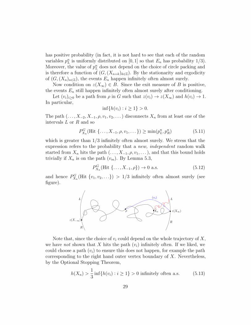
has positive probability (in fact, it is not hard to see that each of the randomvariables pnL is uniformly distributed on [0, 1] so that En has probability 1/3).Moreover, the value of pnL does not depend on the choice of circle packing andis therefore a function of (G, (Xn+k)k∈Z). By the stationarity and ergodicityof (G, (Xn)n∈Z), the events En happen infinitely often almost surely.
Now condition on z(X∞) ∈ B. Since the exit measure of B is positive,the events En still happen infinitely often almost surely after conditioning.
Let (vi)i≥0 be a path from ρ in G such that z(vi)→ z(X∞) and h(vi)→ 1.In particular,
infh(vi) : i ≥ 1 > 0.
The path (. . . , X−2, X−1, ρ, v1, v2, . . . ) disconnects Xn from at least one of theintervals L or R and so
PGXn
(Hit . . . , X−1, ρ, v1, . . . ) ≥ min(pnL, pnR) (5.11)
which is greater than 1/3 infinitely often almost surely. We stress that theexpression refers to the probability that a new, independent random walkstarted from Xn hits the path (. . . , X−1, ρ, v1, . . . ), and that this bound holdstrivially if Xn is on the path (vm). By Lemma 5.3,
PGXn
(Hit . . . , X−1, ρ)→ 0 a.s. (5.12)
and hence PGXn
(Hit v1, v2, . . .) > 1/3 infinitely often almost surely (seefigure).
L
R
z(X∞)
z(X−∞)
(vi)
Xn
L
R
ρ
Note that, since the choice of vi could depend on the whole trajectory of X,we have not shown that X hits the path (vi) infinitely often. If we liked, wecould choose a path (vi) to ensure this does not happen, for example the pathcorresponding to the right hand outer vertex boundary of X. Nevertheless,by the Optional Stopping Theorem,
h(Xn) >1
3infh(vi) : i ≥ 1 > 0 infinitely often a.s. (5.13)
29

and hence, by Levy’s 0-1 law, limn→∞ h(Xn) = 1 almost surely as desired.
We remark that this proof is substantially simpler than the proof forthe deterministic bounded degree case. It may be interesting to attempt toadapt the above proof to the deterministic bounded degree case by replacingstationarity of (G, (Xn+k)n∈Z)k∈Z with tightness.
6 Exponential decay of radii and speed in the
hyperbolic metric
We now use the fact that the exit measure is almost surely non-atomic toimprove Lemma 5.1 and deduce that the limit rate of decay of the Euclideanradii along the random walk exists. The key idea is to use a circle packingin the upper half-plane normalised by the limits of two independent randomwalks.
Fix some circle packing C in D. Let ΦX be a Mobius transformation thatmaps D to the upper half-plane H and sends the almost surely distinct limitpoints z(X∞) = limn→∞ z(Xn) and z(X−∞) = limn→∞ z(X−n) to 0 and ∞respectively and consider the upper half-plane packing C = ΦX(C).
Similarly to the proof of non-atomicity in Section 5.2, we now have twoboundary points (0,∞) fixed by the graph G and the path (Xn), so that theresulting circle packing is unique up to scaling. Now, however, the packingdepends on both G and the random walk, so that this new situation is notparadoxical (as it was in Section 5.2 where we ruled out the possibility thatthe exit measure has a single atom).
Proof of Theorem 1.4. We prove the equivalent statement for (G, ρ) reversiblewith E[deg(ρ)] <∞, and may assume that (G, ρ) is ergodic. We fix a circlepacking C = ΦX(C) in H as above, with the doubly infinite random walkfrom ∞ to 0. Let r(v) be the Euclidean radius of the circle correspondingto v in C. The ratio of radii r(Xn)/r(Xn−1) does not depend on the choiceof C, so that these ratios form a stationary ergodic sequence. By the SharpRing Lemma, E[| log(r(X1)/r(ρ))|] ≤ CE[deg(ρ)] <∞, so that the ErgodicTheorem implies that
− 1
nlog
r(Xn)
r(ρ)= − 1
n
n∑1
logr(Xi)
r(Xi−1)
a.s.−−−→n→∞
−E[log
r(X1)
r(ρ)
]. (6.1)
30

Now, since C is the image of C through the Mobius map ΦX , and sinceΦX is conformal at z(X∞),
r(Xn)
r(Xn)→∣∣∣Φ′X (z(X∞)
)∣∣∣ > 0. (6.2)
Therefore
lim− log r(Xn)
n= E
[− log
r(X1)
r(ρ)
](6.3)
and by Lemma 5.1 this limit must be positive.
Next, we relate this to the speed in the hyperbolic metric. First noticethat
lim1
ndhyp(zh(ρ), zh(Xn)) = lim
2
ntanh−1(|zh(Xn)|) = lim− 1
nlog(1−|zh(Xn)|).
The distance from the hyperbolic centre zh(Xn) to the boundary is smallerthan the distance from the Euclidean centre z(Xn) to the boundary, whichin turn is at most the length of the path formed by drawing straight linesbetween the Euclidean centres of the circles along the random walk pathstarting at Xn:
1− |zh(Xn)| ≤ 1− |z(Xn)| ≤∑i≥n
2r(Xi).
Since the radii decay exponentially, taking the limits of the logarithms,
lim inf− log(1− |zh(Xn)|)
n≥ lim
− log r(Xn)
n. (6.4)
To get the corresponding upper bound, notice that, since every circleneighbouring Xn is contained in the open unit disc, 1− |zh(Xn)| is at leastthe radius of the smallest neighbour of Xn. Applying the Sharp Ring Lemma,we have
1− |zh(Xn)| ≥ r(Xn) exp(−C deg(Xn)).
Taking logarithms and passing to the limit,
lim sup− log(1− |zh(Xn)|)
n≤ lim
− log r(Xn)
n+ lim
C deg(Xn)
n
= lim− log r(Xn)
n, (6.5)
where the almost sure limit deg(Xn)/n → 0 follows from E[deg(ρ)] < ∞and Borel-Cantelli. Combining (6.4) and (6.5) gives the desired almost surelimit.
31

7 Extensions
Adding weights. A natural extension of our results concerns weightedtriangulations. Suppose (G, ρ, w) is a unimodular random rooted weightedtriangulation. As in the unweighted case, if E[w(ρ)] is finite then biasingby w(ρ) gives an equivalent random rooted weighted triangulation whichis reversible for the weighted simple random walk [1, Theorem 4.1]. Ourarguments immediately generalise to recover all our main results in theweighted setting provided the following conditions are satisfied.
1. E[w(ρ)] <∞. This allows us to bias to get a reversible random rootedweighted triangulation.
2. E[w(ρ) deg(ρ)] < ∞. After biasing by w(ρ), the expected degree isfinite, allowing us to apply the Ring Lemma together with the ErgodicTheorem as in the proofs of Lemma 5.1 and Theorem 1.4.
3. A version of Theorem 3.2 holds. That is, there exists a percolation ωsuch that the induced network ω has positive Cheeger constant almostsurely. Two natural situations in which this occurs are
(a) when all the weights are positive almost surely. In this situation,we may adapt the proof of Theorem 3.2 by first deleting all edgesof weight less than 1/M and all vertices of total weight greaterthan M before continuing the construction as before.
(b) when the subgraph formed by the edges of positive weight isconnected and is itself invariantly non-amenable. This occurswhen we circle pack planar maps that are not triangulations byfirst adding edges to triangulate them, and consider these edges tobe of weight zero.
When these restrictions are satisfied, the proofs carry through without furthermodification.
Non-simple triangulations. Suppose G is a one-ended planar map. Eachdouble edge and loop in G disconnects G into connected components exactlyone of which is infinite. The simple core core(G) of G is defined by deletingthe finite component contained within each double edge and loop of G beforegluing the double edges together or deleting the loop as appropriate. Ingeneral, it is possible that all of G is deleted by this procedure, but in
32

this case there are infinitely many disjoint vertex cut-sets of size at most 2separating each vertex from infinity, implying that G is VEL parabolic [22].
We may consider core(G) as a percolation on G by, for each pair of adjacentvertices u and v retained in the core, choosing one of the edges in G betweenu and v uniformly to represent the single edge between u and v in core(G).Note that if two retained vertices are connected by a path of deleted vertices,then they are also connected in the core, so that the induced network core(G)defines a weighting w of core(G) (that is, the weight between each pair ofnon-adjacent vertices is zero).
Proposition 7.1. Let G be a one-ended planar map. Then G is VEL hyper-bolic if and only if core(G) is VEL hyperbolic.
Proof. Suppose G is VEL hyperbolic, so that core(G) is non-empty. Letv ∈ core(G). Recall that the vertex extremal length between v and infinity isdefined by
VELG(v →∞) = supm
infm(γ) : γ an infinite simple path from v2
‖m‖2
,
(7.1)where the supremum is over measures m on V (G). If γ is an infinite simplepath in G starting at v, let Ni be subsequence of times of which γ spendsin core(G). Then γNi
∼ γNi+1in core(G) for all i so that γNi
is a path incore(G). Let m be a measure on V (G) and let v ∈ core(G). Then∑
i
m(γNi) ≤
∑i
m(γi)
so that the infimum in (7.1) may be taken over the set of simple paths from vin core(G). Once this is done, we see that the supremum may be taken overonly those m for which m(V \ core(G)) = 0, so that in fact
VELG(v →∞) = VELcore(G)(v →∞)
and in particular core(G) is VEL hyperbolic. Conversely, if core(G) is VELhyperbolic then G is also by monotonicity.
Proposition 7.2. If (G, ρ) is a one-ended unimodular random rooted map,sampling (G, ρ) conditioned on ρ ∈ core(G) gives rise to a unimodular versionof (core(G), ρ, w).
33

Proof. Write E for the expectation associated to the conditioned law of (G, ρ)
and Z = P(ρ ∈ ω). If f :MR≥0•• → R≥0 is a mass transport,
E∑
v∈core(G)
f(core(G), ρ, v, w) = Z−1E∑v∈G
f(core(G), ρ, v, w)1(ρ, v ∈ core(G))
= Z−1E∑v∈G
f(core(G), v, ρ, w)1(ρ, v ∈ core(G))
= E∑
v∈core(G)
f(core(G), v, ρ, w). (7.2)
where we may apply the mass transport principle for (G, ρ) in the secondequality since the isomorphism class of (core(G), u, v, w) is a function of theisomorphism class of (G, u, v).
Whenever ω is a non-empty percolation we have that, by the OptionalStopping Theorem, the bounded harmonic functions on ω are almost surelyin one-to-one correspondence with the bounded harmonic functions on G byrestriction and extension:
hG 7→ hω = hG|ωhω 7→ hG(v) = EG
v [hω(XN0)].
Finally, If E[deg(ρ)2] <∞ then
E[deg(ρ) degcore(ρ)] ≤ E[deg(ρ)21(ρ ∈ core)]P(ρ ∈ core)−1 <∞.
That is, the reversible version of (core(G), ρ, w) has finite expected degree.As a consequence of these considerations, we get the following immediategeneralisation of Theorem 1.3.
Theorem 7.3. Let (G, ρ) be an invariantly non-amenable, one-ended, uni-modular random rooted planar triangulation with E[deg2(ρ)] <∞ and let Cbe a circle packing of core(G) in D. Then the following hold conditional on(G, ρ) almost surely:
1. z(XNn) and zh(XNn) both converge to a point z(XN∞) ∈ ∂D,
2. The law of z(XN∞) has full support and no atoms.
3. ∂D is a realisation of the Poisson boundary of G. That is, for everybounded harmonic function h on G there exists a bounded measurablefunction g : ∂D→ R such that
h(v) = EGv [g(z(XN∞))] .
34

8 Open Problems
Can the identification of the Poisson and geometric boundaries be strengthenedto an identification of the Martin boundary?
Conjecture 8.1. Let (M,ρ) be a reversible random planar map. Then theMartin boundary of M is almost surely homeomorphic to one of
1. A point if M is invariantly amenable.
2. The circle ∂D if M is invariantly non-amenable and one-ended.
3. The space of ends of M if M is invariantly non-amenable and infinitely-ended.
In case (2), the homeomorphism should arise from circle packing a suitabletriangulation associated to M .
Problem 8.2 (Exit measure is Holder continuous). Is it true that under thesetting of Theorem 1.3 there exists a constant c > 0 such that for any intervalI ⊂ ∂D we have
PGρ (z(X∞) ∈ I) ≤ |I|c ?
Problem 8.3 (Dirichlet energy of z). In the bounded degree case, convergenceto the boundary may be shown by observing that the Dirichlet energy of thecentres function z is finite
E(z) =∑u∼v
(z(u)− z(v))2 ≤∑
deg(v)r(v)2 <∞. (8.1)
Is the Dirichlet energy of z almost surely finite for a unimodular randomrooted CP hyperbolic triangulation? This may provide a route to weakeningthe moment assumption in our results.
Acknowledgements
AN is supported by NSERC and NSF grants. GR is supported in partby the Engineering and Physical Sciences Research Council under grantEP/103372X/1 .
All figures of circle packings were drawn using Ken Stephenson’s CirclePacksoftware, see http://www.math.utk.edu/~kens/CirclePack/. We thankKen for his assistance using this software and for useful conversations.
35

References
[1] D. Aldous and R. Lyons. Processes on unimodular random networks.Electron. J. Probab., 12:no. 54, 1454–1508, 2007.
[2] O. Angel. Growth and percolation on the uniform infinite planar trian-gulation. Geom. Funct. Anal., 13(5):935–974, 2003.
[3] O. Angel, M. T. Barlow, O. Gurel-Gurevich, and A. Nachmias. Bound-aries of planar graphs, via circle packings. Ann. Probab., 2013. toappear.
[4] O. Angel, G. Chapuy, N. Curien, and G. Ray. The local limit of unicellularmaps in high genus. Elec. Comm. Prob, 18:1–8, 2013.
[5] O. Angel and N. Curien. Percolations on random maps I: half-planemodels. Ann. Inst. H. Poincare, 2013. To appear.
[6] O. Angel, T. Hutchcroft, A. Nachmias, and G. Ray. A dichotomy forrandom planar maps. In preparation.
[7] O. Angel, A. Nachmias, and G. Ray. Random walks on stochastichyperbolic half planar triangulations. ArXiv e-prints, Aug. 2014.
[8] O. Angel and G. Ray. Classification of half planar maps. Ann. Probab.,2013. To appear.
[9] O. Angel and O. Schramm. Uniform infinite planar triangulations. Comm.Math. Phys., 241(2-3):191–213, 2003.
[10] I. Benjamini and N. Curien. Simple random walk on the uniform infiniteplanar quadrangulation: subdiffusivity via pioneer points. Geom. Funct.Anal., 23(2):501–531, 2013.
[11] I. Benjamini, R. Lyons, and O. Schramm. Percolation perturbationsin potential theory and random walks. In Random walks and discretepotential theory (Cortona, 1997), Sympos. Math., XXXIX, pages 56–84.Cambridge Univ. Press, Cambridge, 1999.
[12] I. Benjamini, E. Paquette, and J. Pfeffer. Anchored expansion, speed,and the hyperbolic Poisson Voronoi tessellation. ArXiv e-prints, Sept.2014.
36
[13] I. Benjamini and O. Schramm. Harmonic functions on planar andalmost planar graphs and manifolds, via circle packings. Invent. Math.,126(3):565–587, 1996.
[14] I. Benjamini and O. Schramm. Random walks and harmonic functions oninfinite planar graphs using square tilings. Ann. Probab., 24(3):1219–1238,1996.
[15] I. Benjamini and O. Schramm. Percolation in the hyperbolic plane, 2000.
[16] I. Benjamini and O. Schramm. Recurrence of distributional limits offinite planar graphs. Electron. J. Probab., 6:no. 23, 1–13, 2001.
[17] N. Curien. Planar stochastic hyperbolic infinite triangulations.arXiv:1401.3297, 2014.
[18] N. Curien and G. Miermont. Uniform infinite planar quadrangulationswith a boundary. Random Structures Algorithms, 2012. to appear.
[19] A. Georgakopoulos. The boundary of a square tiling of a graph coincideswith the poisson boundary. arXiv:1301.1506, 2013.
[20] O. Gurel-Gurevich and A. Nachmias. Recurrence of planar graph limits.Ann. of Math. (2), 177(2):761–781, 2013.
[21] L. J. Hansen. On the Rodin and Sullivan ring lemma. Complex VariablesTheory Appl., 10(1):23–30, 1988.
[22] Z.-X. He and O. Schramm. Hyperbolic and parabolic packings. DiscreteComput. Geom., 14(2):123–149, 1995.
[23] H. Kesten. Symmetric random walks on groups. Trans. Amer. Math.Soc., 92:336–354, 1959.
[24] P. Koebe. Kontaktprobleme der konformen Abbildung. Hirzel, 1936.
[25] R. J. Lipton and R. E. Tarjan. Applications of a planar separator theorem.SIAM J. Comput., 9(3):615–627, 1980.
[26] R. Lyons and Y. Peres. Probability on Trees and Networks. CambridgeUniversity Press. In preparation. Current version available athttp://mypage.iu.edu/~rdlyons/.
37

[27] G. L. Miller, S.-H. Teng, W. Thurston, and S. A. Vavasis. Separators forsphere-packings and nearest neighbor graphs. J. ACM, 44(1):1–29, Jan.1997.
[28] G. Ray. Hyperbolic random maps. PhD thesis, 2014.
[29] B. Rodin and D. Sullivan. The convergence of circle packings to theRiemann mapping. J. Differential Geom., 26(2):349–360, 1987.
[30] S. Rohde. Oded Schramm: From Circle Packing to SLE. Ann. Probab.,39:1621–1667, 2011.
[31] O. Schramm. Rigidity of infinite (circle) packings. J. Amer. Math. Soc.,4(1):127–149, 1991.
[32] K. Stephenson. Introduction to circle packing. Cambridge UniversityPress, Cambridge, 2005. The theory of discrete analytic functions.
[33] W. P. Thurston. The geometry and topology of 3-manifolds. Princetonlecture notes., 1978-1981.
[34] B. Virag. Anchored expansion and random walk. Geom. Funct. Anal.,10(6):1588–1605, 2000.
38


![Taut ideal triangulations of 3–manifolds · Taut ideal triangulations are closely related to angled ideal triangulations, de-fined and studied by Casson, and developed in [4].](https://static.fdocuments.net/doc/165x107/5f93006a3be63401832bb150/taut-ideal-triangulations-of-3amanifolds-taut-ideal-triangulations-are-closely.jpg)