Unemployment Insurance and Job Search in the Great

Recession

Jesse Rothstein∗

University of California, Berkeley and NBER

September 9, 2011

Abstract

Nearly two years after the official end of the "Great Recession," the labor market

remains historically weak. Many commentators have attributed the ongoing weakness

in part to supply-side effects driven by dramatic expansions of Unemployment Insurance

(UI) benefit durations, to as many as 99 weeks. This paper investigates the effect of

these UI extensions on job search and reemployment. I use the longitudinal structure of

the Current Population Survey to construct unemployment exit hazards that vary across

states, over time, and between individuals with differing unemployment durations. I

then use these hazards to explore a variety of comparisons intended to distinguish the

effects of UI extensions from other determinants of employment outcomes.

The various specifications yield quite similar results. UI extensions had significant

but small negative effects on the probability that the eligible unemployed would exit

unemployment, concentrated among the long-term unemployed. The estimates imply

that UI benefit extensions raised the unemployment rate by only about 0.2–0.6 percent-

age points, much less than is implied by previous analyses. Half or more of this effect

is due to reduced labor force exit among the unemployed rather than to the changes in

reemployment rates that are of greater policy concern; some analyses even suggest that

UI extensions, by keeping displaced workers in the labor market, may have increased

the share who were later reemployed.

1 Introduction

While the so-called “Great Recession” officially ended in June 2009, word has not yet reached

the labor market. In August 2011, the unemployment rate remained above nine percent —∗E-mail: rothstein@berkeley.edu. I thank Stephanie Aaronson, David Card, Hank Farber, Lisa Kahn,

John Quigley, David Romer, Gene Smolensky, Rob Valetta, and Till von Wachter for helpful conversations,and participants in seminars at Berkeley and NBER for comments. I gratefully acknowledge research supportfrom the Institute for Research on Labor and Employment and the Center for Equitable Growth, both atUC Berkeley. Ana Rocca provided excellent research assistance. This research draws on my experiencesworking in the Obama Administration in 2009-10, but all opinions expressed herein are my own.

1

it has fallen below that threshold for only 2 of the last 28 months — and over 40% of the

unemployed had been out of work for more than six months.

An important part of the policy response to the Great Recession has been a dramatic

expansion of Unemployment Insurance (UI) benefits. Preexisting law provided for up to

26 weeks of benefits, plus up to 20 additional weeks of "Extended Benefits" (EB) in states

experiencing high unemployment rates. But Congress has frequently authorized additional

weeks on an ad hoc basis in past recessions, and starting in June 2008 it enacted a series of

UI extensions that brought statutory benefit durations to as long as 99 weeks.

Unemployment benefits subsidize continued unemployment. Thus, it seems likely that

the unprecedented UI extensions in 2008 and 2009 have contributed to some degree to the

elevated unemployment rate. However, the magnitude and interpretation of this effect is not

clear. In an op-ed, Barro (2010) presents a “rough” estimate that extensions of UI benefits

contributed 2.7 percentage points to the unemployment rate in June 2010, and Grubb’s

(2011) comprehensive review of the literature leads him to a similar conclusion (p. 34).

Several direct analyses of recent labor force survey data (see, e.g., Mazumder, 2011; Valetta

and Kuang, 2010; Fujita, 2011) find smaller but still substantial effects.

There are two channels by which UI can raise unemployment, however, with very differ-

ent policy implications (Solon, 1979). On the one hand, UI extensions can lead recipients

to reduce their search effort and raise their reservation wages, slowing the transition into

employment. On the other hand, UI benefits – which are available only to those engaged

in active job search – also provide an incentive for continued search for those who might

otherwise have exited the labor force. The latter raises measured unemployment but has no

effect – or possibly even a positive effect – on the reemployment of displaced workers. Based

in part on this observation, Howell and Azizoglu (2011) find “no support” for the view that

UI extensions have reduced employment. Unfortunately, most studies of the effect of UI on

the duration of unemployment have been unable to distinguish the two channels.

Uncovering the causal effect of UI extensions on labor market outcomes is difficult be-

cause these extensions are badly endogenous by design — UI benefits are extended in severe

recessions precisely because it is seen as unreasonable to expect a displaced worker in a weak

labor market to find a job by the expiration of regular benefits. Thus, obtaining a credible

2

estimate of the effect of the recent UI extensions requires a strategy for distinguishing this

effect from the confounding influence of historically weak labor demand.

This paper uses the haphazard roll-out of the EUC and EB programs during the Great

Recession to identify the partial equilibrium effects of the recent UI extensions on the labor

market outcomes of displaced workers. I use the longitudinal structure of the Current

Population Survey to construct hazard rates for unemployment exit, reemployment, and

labor force exit that vary across states, over time, and between individuals displaced at

different dates.

I explore a variety of strategies for isolating the causal effect of UI extensions. One

strategy exploits the gradual rollout and repeated expiration of EUC benefits through suc-

cessive federal legislation to generate variation in benefit durations across labor markets

facing plausibly similar demand conditions. A second exploits state decisions to take up or

decline optional EB provisions that alter the availability of EB benefits, using a “control

function” to distinguish the effects of the economic conditions that define eligibility. Third,

as in Valetta and Kuang (2010), I use UI-ineligible job seekers as a control group for eligible

unemployed workers in the same state-month labor markets. Finally, I exploit differences

in expected eligibility for EUC benefits by date of unemployment, driven by the uneven

way that the EUC program phases out when it expires, to generate variation in UI benefit

durations among UI-eligible workers within state-month cells.

All of the strategies point to broadly similar conclusions. The availability of extended UI

benefits caused small reductions in the probability that unemployed workers exited unem-

ployment, reducing the monthly hazard in the fourth quarter of 2010 — when the average

unemployed worker anticipated a total benefit duration of 65 weeks — by between one and

two percentage points (on a base of 23.0%). Not more than half of the unemployment

exit effect comes from effects on reemployment: My preferred specification indicates that

UI extensions reduced the average monthly reemployment hazard of unemployed displaced

workers in 2010:Q4 by 0.6 percentage points (on a base of 13.4%), and reduced the monthly

labor force exit hazard by 1.0 percentage points (on a base of 9.0%).

The labor force exit effect raises the possibility that UI extensions might actually raise

the employment rate of formerly displaced workers in bad economic times, by extending the

3

time until they abandon their search.1 However, estimating this effect requires strong as-

sumptions. Adopting such assumptions, I simulate the effect of the 2008-2010 UI extensions

on aggregate unemployment and on the long-term unemployment share. All of the estimates

are partial equilibrium, as I assume that reduced job search from one worker has no effect

on the search behavior or job-finding rate of any other worker. This almost certainly leads

me to overstate the effect of UI extensions.

Nevertheless, I find quite small effects. My preferred specification indicates that in

the absence of unemployment insurance extensions, the unemployment rate in December

2010 would have been about 0.3 percentage points lower and the long-term share of the

unemployed would have been about 1.6 percentage points lower, with over half of each effect

coming from reduced labor force exit. Even the specification yielding the largest effects

indicates that UI extensions contributed only 0.6 percentage points to the unemployment

rate. A simulation of the outcomes of workers displaced in the first quarter of 2009 indicates

that UI extensions raised the share who became reemployed by January 2011 by about 1.3

percentage points (on a base of 68%) by reducing the share who exited the labor force.

As this simulation requires an independent risks assumption that is not easily defensible,

it would be premature to conclude that the EUC and EB programs have had net positive

effects on the reemployment of displaced workers. However, it is clear that any negative

effects are quite small.

The remainder of the paper is organized as follows. Section 2 reviews recent labor

market trends and discusses the UI extensions that have been an important part of the

policy response. It also presents a simple model of the effects of UI benefit durations and

discusses existing estimates of the effect of the recent extensions. Section 3 discusses the

longitudinally-linked CPS data that I use to study the effects of UI. Section 4 presents my

empirical strategies for isolating the UI effect. Section 5 presents estimates of the effect of

UI benefit durations on the unemployment exit hazard. Section 6 develops a simulation

methodology that I use to extrapolate these estimates to obtain effects on labor market1In addition, UI may reduce hysteresis by increasing labor force attachment and thereby slowing the

deterioration of job skills. If so, UI extensions could make displaced workers more employable when demandrecovers. A related possibility is that UI extensions may deter displaced workers from claiming disabilitypayments (Duggan and Imberman, 2009; Joint Economic Committee, 2010).

4

aggregates, and presents results. Section 7 concludes.

2 The Labor Market and Unemployment Insurance in the

Great Recession

2.1 Labor market trends

The recession officially began in December 2007, but the downturn was slow at first: Sea-

sonally adjusted U.S. real GDP fell at an annual rate of only 0.7 percent in the first quarter

of 2008. Conditions worsened sharply in late 2008 and GDP contracted at an annual rate

of 6.8 percent in the fourth quarter.

The labor market downturn also began slowly. Figure 1 shows that the unemployment

rate began trending up in 2007, but remained only 5.8% in July 2008. Over the next year,

however, it rose 3.7 percentage points, to 9.5 percent, and has fallen below 9 percent in only

two months since. Employment data show similar trends: Nonfarm payroll employment

rose through most of 2007, fell by 738,000 in the first half of 2008, and then fell by nearly

6.8 million over the next year. Job losses continued at slower rates in the second half of

2009, followed by modest and inconsistent growth in 2010. As of August 2011, employment

remained 6.9 million below its pre-recession peak.

Figure 1 also shows the long-term unemployment rate, defined as the share of the un-

employed who have been out of work for six months or more. It generally lags the overall

unemployment rate by about six months or perhaps a bit more: It began to increase slowly

in early 2008 and much more quickly in late 2008, reaching a peak around 45% in early 2010

and remaining mostly stable since then.

Figures 2A and 2B illustrate gross labor market flows over the course of the reces-

sion. These are obtained from two sources: The Job Openings and Labor Turnover Survey

(JOLTS), which derives from employer reports, and the gross flows data computed by the

Bureau of Labor Statistics from matched monthly Current Population Survey (CPS) house-

hold data discussed at length below. Figure 2A shows flows out of work: Quits and layoffs

from the JOLTS (“other separations,” including retirements, are not shown), and gross em-

5

ployment to unemployment (E-U) flows from the CPS. Figure 2B shows flows into work:

Hires from the JOLTS and unemployment to employment (U-E) flows from the CPS. It also

shows unemployment to non-participation (U-N) flows, with both the U-E and U-N flows

expressed as shares of the previous month’s unemployed population.

Together, Figures 2A and 2B shed a good deal of light on the dynamics of the rise

and stagnation of the unemployment rate.2 Figure 2A shows that layoffs spiked and quits

collapsed in late 2008, indicating an extreme weakening of labor demand; interestingly, the

decline in quits seems to have preceded the increase in layoffs by several months. Not

surprisingly, the number of monthly employment-to-unemployment transitions increased by

about one-third over the course of 2008. Layoffs returned to (or even below) normal levels

in late 2009, but quits remained just over half of their pre-recession level and E-U flows

remained high, suggesting that weak demand continued to dissuade workers from leaving

their jobs and to impede the usual quick transition of displaced workers into new jobs.

Turning to Figure 2B, we see that the collapse in new hires was more gradual than

the spike in layoffs and began much earlier, in late 2007. The rate at which unemployed

workers transitioned into employment also began to decline at this time, then fell much

more sharply in late 2008. Recall that the rapid run-up in long-term unemployment was

in mid-2009, roughly six months later, again suggesting that the usual process by which

displaced workers are recycled into new jobs was substantially disrupted around the time

of the financial crisis. U-E flows remain very low through the present day. Finally, the

U-N flow rate fell rather than rose during the recession, despite weak labor demand which

might plausibly have led unemployed workers to become discouraged. This is plausibly

a consequence of unemployment insurance benefit extensions, which created incentives for

ongoing search even if the prospect of finding a job was remote.

2.2 The policy response

Congress responded quickly to the deteriorating labor market, authorizing Emergency Un-

employment Compensation (EUC) benefits in June 2008, but proceeded in fits and starts2See Elsby et al. (2010) for a more detailed examination of these and other aggregate data.

6

thereafter.3 The June 2008 legislation made 13 weeks of EUC benefits available to any-

one who exhausted his regular benefits before March 28, 2009. The EUC program was

subsequently extended and expanded several times by Congressional action:

• In November 2008, an additional seven weeks were added to what was thereafter

referred to as “Tier I” of EUC benefits. On top of this, 13 weeks of Tier II benefits

were made available in states with unemployment rates above 6 percent, permitting

as many as 33 weeks of EUC benefits in those states.

• In February 2009, the expiration of the EUC program was extended to December 26,

2009.

• In November 2009, Tier II benefits were extended by one week and made unconditional.

13 weeks of Tier III benefits were added in states with unemployment rates above

6 percent, and six further weeks of Tier IV benefits were provided for states with

unemployment rates above 8.5 percent. In such states, the four tiers together provided

as many as 53 weeks of benefits. However, the program expiration date was unchanged

from December 26, 2009.

• On December 19, 2009, one week before the scheduled expiration, the expiration date

was pushed back to February 28, 2010.

• On March 2, 2010, the expiration date was extended to April 5 of that year, retroactive

to the February 28 expiration.

• On April 15, 2010, the expiration date was again retroactively extended to June 2.

• On July 22, 2010, seven weeks after the June 2 expiration, the EUC program was once

again retroactively extended to November 30.

• On December 17, 2010, the expiration date was extended, again retroactively, to Jan-

uary 3, 2012.3This discussion draws heavily on Fujita (2010). I neglect a number of complexities of the UI program. In

particular, claimants whose previous jobs were short are not eligible for the full 26 weeks of regular benefitsor for the indicated number of weeks of EUC benefits. There are also important complexities having to dowith unemployment spells interrupted by periods of employment or inactivity.

7

On top of these EUC program expansions and extensions, the American Recovery and

Reinvestment Act of (February) 2009 made several other changes to the UI program: It

provided for $25 in extra weekly benefits to each recipient, for full Federal funding of the EB

program (formerly split equally between state and federal budgets), for tax deductibility of

a portion of UI benefits, and for somewhat expanded eligibility for benefits. The EB funding

change induced a number of states to begin participating in the program and to adopt its

optional, more generous triggers, further adding to the number of weeks of benefits available

to unemployed workers.

Combining 26 weeks of regular benefits, up to 53 weeks of EUC, and as many as 20 weeks

of EB, statutory benefit durations have reached as long as 99 weeks. However, this overstates

the number of weeks that any individual claimant could expect. According to EUC program

rules, after the program expires participants can draw out the remaining benefits from any

tier already started but cannot transition to the next tier. Throughout 2010, the expiration

date of the program was never more than a few months away. Thus, although as many 99

weeks of EUC benefits were available in statute starting in November 2009, no individual

exhausting her regular benefits in 2010 could have anticipated being able to draw benefits

from EUC Tiers III or IV absent further congressional action, keeping maximum anticipated

benefit durations below 70 for anyone who was not already out of work for a year or more.

It is not clear how to model workers’ expectations in the weeks leading up to a scheduled

EUC expiration. They might reasonably have expected an extension, if only to smooth

the “cliff” in benefits that would otherwise be created. However, each extension has been

highly controversial, facing determined opposition and filibusters in the Senate. It would

have been quite a leap of faith in mid 2010, in the midst of a Republican resurgence, for an

unemployed worker to assume that the program would be extended beyond its November 30

expiration. Moreover, even a worker who foresaw an eventual extension might (reasonably)

have expected a gap in benefits between the program’s expiration and its eventual reautho-

rization. For a UI recipient facing binding credit constraints, benefits paid retroactively are

much less valuable than those paid on time. I thus assume throughout that workers assume

at all times that the EUC program will expire as scheduled according to then-current law

8

and that neither state nor federal legislation will change the terms of the program.4 I also

assume that workers forecast that their states will neither trigger on to EUC tiers or EB

benefits that they are not yet on nor trigger off of those that they are currently on.

Figure 3 provides two ways of looking at the evolution of UI durations. The left panel

shows estimates for the state with the longest benefit durations at any point in time. After

late 2008, this is a state qualifying for 20 weeks of EB benefits and all extant EUC tiers. The

right panel shows the (unweighted) average across states. In each panel, the short dashes

show the maximum number of weeks available by statute over time, while the long dashes

and the solid line show the expectations of a newly displaced worker and of a worker who

has just exhausted her regular benefits, respectively.

The “statutory” series shows a rapid run-up, due primarily to EUC expansions and

secondarily to EB triggers, in 2008 and throughout 2009, followed by repeated collapses in

2010 when the EUC program temporarily sunsetted. However, the other two series show

much more gradual changes from the perspective of individuals early in their allowed benefits.

Newly displaced workers who did not expect further legislative action would have seen the

EUC program as largely irrelevant for most of its existence, as only for a brief period in early

2009 and then after December 2010 was the expiration of the EUC program farther away

than the 26 weeks it would take for a newly displaced worker to exhaust his regular benefits.

Workers already exhausting their regular benefits, by contrast, would have anticipated at

least Tier I benefits at all times except during the temporary sunsets. Even these workers,

however, could not look forward to Tier II, III, or IV benefits for most of the history of the

program. It is only in December 2010 and the very beginning of 2011 that any such worker

could anticipate eligibility for Tier IV benefits. A final feature to notice is that the average

state was quite close to the maximum from 2009 on, as most states had adopted at least 13

weeks of EB benefits and most had hit their triggers.4Farber and Valletta (2011), in an analysis otherwise similar to this one, assume instead that workers act

as if they anticipate seamless extensions. They obtain similar results to those here.

9

2.3 A model of job search and UI durations

To fix ideas, I develop a simple discrete time model of job search with exogenous wages and

time-limited unemployment insurance. The model yields two main results: First, search

intensity rises as UI benefit expiration approaches, and is higher for UI exhaustees than for

those still receiving benefits. Thus, an extension of UI benefits reduces the reemployment

chances of searching individuals, both those who have exhausted their regular benefits and

those who are still drawing regular benefits and thus not directly affected by the extension.

Second, when UI benefit receipt is conditioned on continuing job search, benefit extensions

can raise the probability of search continuation. Both results imply positive effects of benefit

extensions on measured unemployment. However, because the second channel can increase

search, the net effect on the reemployment of displaced workers is ambiguous.

I assume that individuals cannot borrow or save.5 The income — and therefore the

consumption — of an unemployed individual is b if she receives UI benefits and is 0 otherwise.

Her per-period flow utility is u (c) − s, where c is her consumption and s is the amount of

effort she devotes to search. If she finds a job, it will be permanent and will offer an

exogenous wage w > b and flow utility u (w). The probability that she finds a job in a

period is an increasing function of search effort, p (s), with p� (s) > 0, p�� (s) < 0, p (0) = 0,

p� (0) = ∞, and p (s) < 1 for all s. Although p (s) might naturally be modeled as a function of

changing labor market conditions, to avoid excessive complexity from dynamic anticipation

effects I assume that job seekers treat it as fixed. I assume that unemployment benefits are

available for up to D periods of unemployment. Initially, I model these as conditional only

on continued unemployment; later, I condition also on a minimum level of search effort.

With these assumptions, the value function of someone who has a job at the beginning

of a period is VE =�∞

t=0 δtu (w), where 1 − δ is the per-period discount rate. The value

function of an unemployed individual depends on her search effort and on the number of5Chetty (2008) finds that much of the search effect of unemployment insurance is concentrated among

those who are credit constrained, and also that lump-sum severance pay has a similar effect to UI benefitextensions (see also Card et al., 2007a). Both results suggest that the income effects of UI benefits may bemore important than the substitution effects.

10

weeks of benefits remaining, d:

VU (s, d) =

u (b)− s+ δ [p (s)VE + (1− p (s))VU (d− 1)] if d > 0

u (0)− s+ δ [p (s)VE + (1− p (s))VU (0)] if d = 0

(1)

where VU (d) ≡ maxs VU (s, d). Search effort is chosen to maximize VU (s, d). The optimal

choice will satisfy

p� (s∗d) =1

δ (VE − VU (0))

for d ∈ {0, 1} and

p� (s∗d) =1

δ (VE − VU (d− 1))

for d > 1. The following results are proved in an appendix.

Proposition 1. The value function VU (d) is increasing in d: VU (d+ 1) > VU (d) for all

d ≥ 0.

Proposition 2. Search effort increases as exhaustion approaches, reaching its final level in

the penultimate period of benefit receipt: s∗d+1 < s∗d < s∗1 = s∗0 for all d ≥ 2.

Proposition 2 implies that unemployment insurance extensions will reduce job-finding

rates at all unemployment durations below the new maximum benefit duration D and will

shift the time-until-reemployment distribution rightward. The relative magnitude of the

effect at different unemployment durations depends on the shape of the p () function, but

under plausible parameterizations�s∗d−1 − s∗d

�declines with d so benefit extensions will have

the largest effects on the search effort of those who would otherwise be at or near exhaustion.

But these results neglect the impact of UI job search requirements. To incorporate them,

I assume that an individual is considered a part of the labor force and therefore eligible to

receive UI benefits only if his search effort is at least θ > 0; otherwise, he receives no benefit

but preserves his remaining benefit entitlement.6 The value function is now:6It is mathematically convenient but not substantively important that the range of s for which benefits

are paid be closed on the left. Thus, I assume θ is strictly positive, although it can be arbitrarily close tozero.

11

VU (s, d) =

u (b)− s+ δ�p (s)VE + (1− p (s)) VU (d− 1)

�if d > 0 and s ≥ θ

u (0)− s+ δ�p (s)VE + (1− p (s)) VU (d)

�if d = 0 or s < θ

(2)

Unemployment benefits may deter an unemployed individual from exiting the labor

force if search productivity is low (i.e., if p� (θ) < 1δ(VE−VU (d−1))) and if benefit levels are

high relative to θ. It can be shown that:

Proposition 3. Any individual who chooses search effort s ≥ θ with d weeks of benefits

remaining would also choose s ≥ θ with d� weeks remaining, for all d, d� > 0.

Intuitively, an individual who chooses s < θ when her UI entitlement has not yet been

exhausted faces identical optimization problems in both the preceding and the following

weeks. Thus, labor force exit occurs either immediately after a job loss or upon exhaus-

tion of UI benefits; UI benefit extensions reduce non-participation among those who would

otherwise have exhausted their benefits. This implies that the net effect of UI extensions

when job search requirements are enforced is ambiguous: Those who would have searched

intensively will reduce their search effort, while some of those who would have dropped out

of the labor force will increase their effort. The relative strength of these two effects is

likely to vary over the business cycle: When labor demand is strong and search productivity

therefore high, the negative effect is likely to dominate, but when search productivity is low

the former may be more important.

Finally, it is worth mentioning two important factors that are not captured by this model.

First, p (s) may evolve over the business cycle. If p (s) is temporarily low but expected to

recover later, UI extensions might keep individuals searching through the low-demand period.

If search productivity is increasing in past search effort, as is implied by many discussions of

hysteresis, this could lead to higher employment when the economy recovers. Even without

state dependence in p (s), UI extensions may bring discouraged workers back into the labor

force earlier in the business cycle upswing. Second, I do not model general equilibrium effects,

or “crowding out.” Reduced search effort from one person likely increases the productivity

of search for all others — if a UI recipient does not take an available job, this merely makes

12

the job available to someone else. This kind of search externality is particularly important

if the labor market is “demand constrained,” but arises anytime labor demand is downward

sloping. In the presence of search externalities, partial-equilibrium estimates of the effect of

UI extensions on reemployment probabilities will overstate the general equilibrium effects.

2.4 Prior estimates of the effect of UI extensions in the Great Recession

There have been a number of estimates of the effect of the recent UI extensions on labor

market outcomes. All involve extrapolations from pre-recession estimates of the effect of UI

durations or from pre-recession unemployment exit rates. Barro (2010) assumes that in the

absence of the extensions the long-term unemployment rate would have held to the 24.5%

level seen in 1983.7 This leads him to conclude that the unemployment rate would have

been 2.7 percentage points lower in June 2010 than it actually was.

Mazumder (2011) uses estimates of the effect of UI durations from Katz and Meyer

(1990a) and Card and Levine (2000) to conclude that UI extensions contributed 0.8 to

1.2 percentage points to the unemployment rate in February 2011.8 But UI durations in

the current recession are longer and labor market conditions are different in a variety of

ways than in the periods used for the earlier studies. The effect of UI durations in the

earlier estimates largely reflects a spike in the unemployment exit hazard in the weeks

immediately prior to benefit exhaustion. Katz and Meyer (1990b) find that much of this

spike is attributable to laid off workers recalled to their previous job; these recalls are thought

to have become much less common in recent years. Card et al. (2007a,b) suggest that much of

the remaining spike is attributable to labor force exit rather than reemployment, highlighting

the importance of distinguishing these two channels.9

Fujita (2011) extrapolates from reemployment and labor force exit hazards observed in

2004-2007 to infer counterfactual hazards in 2009-2010 had UI benefits not been extended.7This ignores the long-run secular increase in the long-term unemployment rate, which at the business

cycle peak in December 2007 was more than double its level at the January 1980 peak (18.9% vs. 8.3%).8Aaronson et al. (2010), Fujita (2010), and Elsby et al. (2010) use similar strategies and obtain similar

results.9Another potential explanation for large spikes in at least some of the earlier studies is heaping in reported

unemployment durations. Katz (1986) and Sider (1985) suggest that in retrospective reports much of theobserved heaping — especially prominent at 26 weeks (or 6 months), the duration of regular UI benefits —reflects recall error or other factors (Card and Levine, 2000) rather than UI effects.

13

To absorb confounding effects from changes in labor demand, he controls linearly for the job

vacancy rate. He finds larger effects of UI extensions on unemployment than does Mazumder

(2011), primarily attributable to reduced reemployment rather than reduced labor force exit.

However, these conclusions are based on the extrapolated effects of a reduction in the job

vacancy rate that is roughly twice as large as the range observed in the earlier period.

Valetta and Kuang (2010) contrast changes in the unemployment durations of job-losers

— many of whom are eligible for UI benefits — and job-leavers — who are not — over the

course of the recession, in principle identifying the UI effect in the presence of arbitrary

changes in demand conditions. They conclude that UI extensions raised the unemployment

rate by 0.8 percentage points in mid-2010. However, the collapse in the quit rate seen in

Figure 2A suggests that UI extensions may not be the only source of changes in the relative

outcomes of job losers and job leavers. If the remaining job leavers come largely from sectors

where job openings are plentiful while job losers come from those hit hard by the recession

(e.g., construction), the comparison between them will overstate any negative effect of UI

extensions.

Finally, Grubb’s (2011) and Howell and Azizoglu’s (2011) literature reviews come to

very different conclusions about the likely effect of the current extensions. Grubb concludes

that UI extensions are responsible for much of the increase in unemployment over the re-

cession, while Howell and Azizoglu conclude that any effect is much smaller and primarily

attributable to reduced labor force exit induced by the UI job search requirement.

3 Data

I use the Current Population Survey (CPS) rotating panel to measure the labor market

outcomes of a large sample of unemployed workers in the very recent past. Three-quarters

of each month’s CPS sample is targeted for another interview the following month, and it is

possible to match over 70% of monthly respondents (94% of the attempted reinterviews) to

employment statuses in the following month. (The most important source of mismatches is

individuals who move, who are not followed.) This permits me to measure one-month-later

employment outcomes for roughly 4,000 unemployed workers each month during the Great

14

Recession, and thereby to construct monthly reemployment and labor force exit hazards

that vary by state, date of unemployment, and unemployment duration.

The CPS data have advantages and disadvantages relative to other data that have been

used to study UI effects. Advantages include larger and more current samples, the ability to

track outcomes for individuals who have exhausted their UI benefits or who are not eligible,

and the ability to distinguish reemployment from labor force exit.

These are offset by important limitations. First, the monthly CPS does not contain

measures of UI eligibility or receipt. Past research has found that only about half of the

unemployed actually receive UI benefits (Anderson and Meyer, 1997). This appears to

have risen somewhat in the current recession; I estimate that over half of displaced work-

ers unemployed more than three months in early 2010 received UI benefits.10 Although

the participation rate is far less than 100%, I simulate remaining benefit durations for all

displaced workers, assuming that each is eligible for full benefits. As I estimate relatively

sparse specifications without extensive individual controls, the estimates can be seen as the

“reduced form” average effect of available durations on the labor market outcomes of all

displaced workers, pooling recipients and non-recipients. To implement the simulation, I

match the CPS data to detailed information about the availability of EUC and EB benefits

at a state-week level and compute eligibility for benefits in each week between the time of

displacement and the initial CPS interview (including those paid retroactively due to de-

layed reauthorizations). I assume that one week of eligibility has been used for each week

of covered unemployment (including retroactive coverage due to delayed reauthorizations).

In modeling expectations for benefits subsequent to the CPS interview, I assume that

the individual anticipates no further legislative action or “triggering” of benefits on or off

after that date, as in Figure 3. Insofar as unemployed individuals are able to forecast future

legislation, I may understate the duration of expected benefits and overstate the amount

of variation across unemployment entry cohorts within the same state. It is unclear in

which direction we would expect this nonclassical measurement error to bias my results.10Observations in February, March, and April can be matched to data from the Annual Demographic

Survey, which includes questions about UI income in the previous calendar year. In early 2010, 56% ofjob-leavers whose unemployment spells appear to have started before December 1, 2009 reported non-zeroUI income, up from 39% in early 2005.

15

However, in a paper written simultaneously with this one Farber and Valletta (2011) use

similar identification strategies along with an assumption that individuals perfectly forecast

reauthorization of the EUC program, and obtain very similar results to those here.

A second limitation of the CPS data is that employment status and unemployment

durations are self-reported, and respondents may not fully understand the official definitions.

Officially, someone who is out of work, is available to start work, and has actively looked for

work at least once in the last four weeks should be classified as “unemployed,” with a duration

of unemployment reaching back to the last time he/she was not in this state. Someone who

has not actively searched or is unavailable to start a job is out of the labor force. But the line

between unemployment and non-participation can be blurry, particularly when there are few

suitable job openings to which to apply or when job search is intermittent. The data suggest

that reported unemployment durations often stretch across periods of non-participation

or short-term employment back to the perceived “true” beginning of the unemployment

spell. Reinterviews with CPS respondents in the 1980s indicate important misclassification

of labor force status, particularly for unemployed individuals who are often misclassified

as out of the labor force. This leads to substantial overstatement of unemployment exit

probabilities (Poterba and Summers, 1984, 1995; Abowd and Zellner, 1985).11 Relatedly,

examination of the unemployment duration distributions indicates substantial heaping at

monthly, semi-annual, and annual frequencies, suggesting that many respondents round their

unemployment durations.

To minimize the misclassification problem, my primary estimates count someone who

is observed to exit unemployment in one month but return the following month — that is,

someone whose three-month trajectory is U-N-U or U-E-U — as a non-exit.12 This means

that I can only measure unemployment exits for observations with at least two subsequent

interviews. I have also estimated alternative specifications that count all measured exits or

that exclude many of the “heaped” observations, with similar results.13 I discuss these issues11CPS procedures were altered in 1994, in part to reduce classification error. However, the Census Bureau

has not released data from reinterview surveys since the redesign, so it is unclear how successful this was.12Fujita (2011) also recodes some U-N-U trajectories as U-U-U.13I am unable to address a related potential problem: although the CPS data collection is independent

of that used to enforce job search requirements, these requirements may lead some true non-participants tomisreport themselves as active searchers. This may lead me to overstate the true impact of UI durations onlabor force participation decisions.

16

at greater length in Section 6.

Finally, the CPS does not attempt to track respondents who change residences between

interviews. If UI eligibility affects the propensity to move, this could bias my estimates in

unknown ways. Although the mobility rate may have fallen over the course of the recession

(Frey, 2009; Kaplan and Schulhofer-Wohl, 2011), my ability to match a CPS respondent

to a follow-up outcome does not appear to be correlated with my UI duration measures,

conditional on the covariates discussed below.

Table 1 presents summary statistics for my full CPS sample, which pools data for inter-

views between May 2004 and January 2011, matched to subsequent interviews in each of the

next two months. (Rotation groups that would not have been targeted for two follow-up in-

terviews are excluded.) Figure 4 presents average monthly exit probabilities for unemployed

workers who report having been displaced from their previous jobs (as distinct from new

entrants to the labor force, reentrants, and voluntary job leavers) over the sample period.

The overall exit hazard fell from about 40% in mid 2007 to about 25% throughout 2009

and 2010.14 The Figure also reports exit hazards for those unemployed 0-13 weeks and 26

weeks or more. The hazard is higher for the short-term than for the long-term unemployed.

However, both series fell similarly to the overall average in 2007 and 2008, suggesting that

only a small portion of the overall exit hazard decline can be due to composition effects

arising from the increased share of long-term unemployed with low exit rates.

4 Empirical Strategy

The matched CPS data allow me to measure whether an unemployed individual exits un-

employment over the next month, but do not allow me to follow those who do not exit to

the end of their spells. I thus focus on modeling the exit hazard directly. I assume the

monthly hazard follows a logistic function. To distinguish between the different forms of

unemployment exit, I turn to a multinomial logit model that takes reemployment, labor

force exit, and continued unemployment as possible outcomes.

Let nist be the number of weeks that unemployed person i in state s in month t has been14This is a lower exit rate than is apparent in the BLS gross flows data, which also derive from matched

CPS samples but do not incorporate my adjustment for U-N-U trajectories.

17

unemployed (censored at 99); let Dist be the total number of weeks of benefits available to

her, including the nist weeks already used as well as weeks she expects to be able to draw

in the future; and let Zst be a measure of economic conditions. Using a sample of displaced

workers, I estimate specifications of the form:

ln

�λist

1− λist

�= Distθ + Pn (nist; γ) + PZ (Zst; δ) + αs + ηt. (3)

λist is the probability that the individual exits unemployment by month t + 1; αs and ηt

are fixed effects for states and months; and Pn and PZ are flexible polynomials. This can

be seen as a maximum likelihood estimator of a censored survival model with stock-based

sampling and a logistic exit hazard, with each individual observed for only two periods.15

However, as I discuss below , modeling survival functions in the CPS data is challenging due

to inconsistencies between stock-based and flow-based measures of survival. In Section 6, I

develop a simulation approach to recovering survival curves from the estimated exit hazards

that are consistent with the observed duration profile. For now, I focus on modeling the

hazards themselves.

After some experimentation, I settled on the following parameterization of Pn:

Pn (nist; γ) = nistγ1 + n2istγ2 + n−1

istγ3 + 1 (nist ≤ 1) γ4. (4)

This appears flexible enough to capture most of the duration pattern. I have also estimated

versions of (3) that include a full set of dummy variables for all 100 possible values of nist,

with little effect on the results.

As discussed above, the main challenge in identifying the effect of Dist is that it covaries

importantly with labor demand conditions. My first empirical strategy exploits the haphaz-

ard roll-out of EUC, the discontinuous triggers in EUC and EB, and the repeated expiration

and renewal of the federal authorizing legislation to generate variation in the duration of15In principle, individuals can be followed for more than two periods in the CPS data. Accounting for this

would give rise to a somewhat more complex likelihood function. I treat an individual observed for threeperiods as two distinct observations, one on exit from period 1 to period 2 and another on exit from period2 to period 3 (if she survives in unemployment in period 2), allowing for dependence of the error term acrossthe observations.

18

UI benefits among labor markets experiencing plausibly similar economic conditions. This

requires absorbing labor demand conditions through the PZ function. In my preferred spec-

ification, PZ is a cubic polynomial in the state unemployment rate. I also explore richer

specifications that control as well for cubics in the insured unemployment rate — an alter-

native measure of unemployment based only on UI-eligible workers — and the number of

new UI claims in the CPS week (expressed as a share of the employed, eligible population).

Note that labor demand is likely negatively correlated with the availability of benefits, so

specifications of PZ that do not adequately capture demand conditions will likely lead me

to overstate the negative effect of UI benefits on job-finding.

My second strategy narrows in on the variation coming from state decisions about which

EB triggers to adopt, using a control function to absorb all other variation in Dist. I

augment (3) with controls for the availability of EB benefits under maximal and minimal

state participation in EB, along with indicators for the status of each of the four EB triggers

and for the actual number of EUC weeks available.16 With these controls, the only variation

in Dist should come from differences among states in similar economic circumstances in take-

up of the optional EB triggers.

Both of these strategies rely on parametric controls to ensure that Dist is conditionally

uncorrelated with labor demand. A third strategy uses job seekers who are not eligible for

UI, either because they are new entrants to the labor market or because they left their former

jobs voluntarily, to control non-parametrically for state labor market conditions (Valetta and

Kuang, 2010; Farber and Valletta, 2011). Using a sample that pools all of the unemployed,

I estimate:

ln

�λist

1− λist

�= Distθ + Pn (nist, eist; γ) + eistPZ (Zst; δ) + αst, (5)

16During the period covered by my sample, trigger 1 is “on” when the 13-week moving average of theinsured unemployment rate (IUR) is at least 5% and above 120% of the maximum of its values one year andtwo years prior. Trigger 2 is on when the IUR is at least 6%, without the lookback provision. Trigger 3 ison when the three-month moving average of the total unemployment rate (TUR; the traditional measure)exceeds 6.5% and is above 110% of the minimum of its values one year and two years prior. Trigger 4 is onwhen the TUR exceeds 8%, with a similar lookback. Trigger 1 applies to all states; states can opt to usetrigger 2 or trigger 3 as well, but if they use trigger 3 they must also provide 20 weeks (in place of the usual 13)of EB benefits if trigger 4 is on. My minimal and maximal simulated EB eligibility measures are an indicatorfor trigger 1 being on and an indicator for one of triggers 1, 2, and 3 being on; these simulated measures,following program rules, can change status no more than once in 13 weeks. See National Employment LawProject (2011) and Federal-State Extended Unemployment Compensation Act of 1970 (Undated).

19

where αst is a full set of state-month indicators and eist is an indicator for whether individual

i is a job loser (and therefore presumptively UI-eligible). Pn(nist, eist; γ) represents the full

interaction of the unemployment duration controls (4) with the eligibility indicator, while

eistPZ(Zst; δ) indicates that the relative labor market outcomes of job losers and other

unemployed are allowed to vary parametrically with observed labor market conditions. The

UI duration coefficient θ is identified from covariance between UI extensions and changes in

the relative unemployment exit rates of job losers and other unemployed, over and above

that which can be explained via a cubic in the unemployment rate. This specification has

the advantage that it does not rely on parametric controls to measure the absolute effect

of economic conditions on job-finding rates. However, recall that Figure 2A indicated that

the quit rate has been low throughout the recession. If the ineligible unemployed during the

period when benefits were extended are disproportionately composed of people who have

relatively good employment prospects, the evolving prospects of the population of ineligibles

may not be a good guide to those of eligibles, leading specification (5) to overstate the causal

effect of UI benefits.

Equations (3) and (5) model the effect of UI extensions as a constant shift in the log

odds of unemployment exit, reemployment, or labor force exit. But it seems more likely

that these extensions would have larger effects on the job search behavior of those who

directly benefit from them than on those who anticipate being eligible for extended benefits

many months in the future. I explore this in two ways. First, I allow the θ coefficient to

vary with nist, the length of the unemployment spell, allowing for different effects on those

unemployed for more than or less than 26 weeks. Second, following the result in Section

2.3 that the intensity of search effort increases as benefit exhaustion approaches, I turn to a

fourth estimation strategy that specifies the UI effect in terms of the time to exhaustion:

ln

�λist

1− λist

�= f (dist; θ) +

99�

v=0

1 (nist = v) γv + αst. (6)

Here, dist = max {0, Dist − nist} represents the number of weeks of benefits remaining,

with f (·; θ) a flexible function; I impose only the normalization that f(0; θ) = 0, corre-

sponding to an assumption that UI extensions have no effect on job searchers who have

20

already exhausted even their extended benefits. The second term in (6) is a full set of indi-

cators for unemployment duration, and the third is a full set of state-by-month indicators.

The effect of dist is identified from comparisons among individuals of different unemploy-

ment durations in the same state-month labor market. There are two sources of variation

that allow separate identification of the effects of d and n without parametric restrictions,

using a sample solely consisting of displaced workers. First, across-st variation in benefit

availability has one-for-one effects on dist for those who have not yet exhausted benefits

but not for those who have. Second, the EUC expiration rules mean that the addition of

new EUC tiers extends d for those who will transition onto the new tiers before the EUC

program expires but not for those with lower nist who expect the program to have expired

before they reach the new tiers.

5 Estimates

Panel A of Table 2 presents logit estimates of equation (3), with standard errors clustered

at the state level. The table shows the unemployment duration coefficient and its standard

error. I also show the estimated effect of the UI extensions on the average exit hazard

in the fourth quarter of 2010, computed as the difference between the average fitted exit

probability and the fitted probability implied by the model if benefit durations had been

held fixed at 26 weeks. 17 Column 1 is estimated using only displaced workers who are

presumed to be eligible for UI benefits, and includes state and month fixed effects, the nist

controls indicated by (4), and a linear control for the state unemployment rate. It indicates

a significant, albeit small effect of UI benefit durations on the probability of unemployment

exit, with a net effect of the UI extensions on the 2010:Q4 exit rate of -1.7 percentage points

(on a base of 22.4%). Columns 2, 3, and 4 add additional controls: First a cubic in the

state unemployment rate in column 3, then cubics in two other measures of slackness —

the number of UI claimants and the number of new UI claims, each expressed as a share

of insured employment — in column 3, and finally a cubic in the state employment growth17Strictly, I use observations from the September–November surveys. December observations are excluded

because the EUC program had expired and not yet been renewed at the time of the December survey; seeSection 2.2.

21

rate, in column 4. These specifications indicate modestly larger UI duration effects.

Column 5 turns to my second strategy, using a “control function” to isolate variation in

benefit durations coming from state decisions about which version of the EB triggers to use.

I augment the specification from Column 2 with controls for the number of weeks of EUC

benefits, for the status of each of the four EB triggers, and for simulated EB benefits under

the most and least generous versions of the triggers. This leaves little variation in the D

variable and produces large standard errors, but the point estimate is similar to those in

columns 1–4.

Finally, column 6 turns to my third strategy, returning to my preferred outcome variable

and adding to the sample over 60,000 unemployed individuals who left their jobs voluntarily

or are new entrants to the labor force and are therefore not eligible for UI benefits. As

indicated by equation (5), this specification includes state-by-month fixed effects.18 plus

controls for separate duration and unemployment rate effects for job losers relative to the

other unemployed. The UI effect is notably larger in this column than in the earlier spec-

ifications, perhaps indicating that the UI-ineligible unemployed are not an ideal control

group for the eligible unemployed during the recession. However, even in this specification

the estimates indicate that the UI extensions reduced the monthly exit hazard by only 3.7

percentage points. By comparison Figure 4 indicates that the exit hazard fell by about 20

percentage points between 2006 and 2009.

Panel B of Table 2 loosens the specifications from Panel A, allowing Dist to have distinct

effects on those unemployed more and less than 26 weeks. The negative effect of D on

unemployment exit is found to be heavily concentrated among those unemployed 26 weeks or

more, with only one of the six estimates of the effect on shorter-term unemployed significantly

different from zero. The implied effects of UI extensions on exit hazards are smaller than

those in Panel A in columns 1–4, but larger in columns 5 and 6. Now column 5 shows a UI

effect on the 2010:Q4 exit rate nearly twice as large as in column 4, but the standard errors

indicate that the difference is not statistically significant.

Table 3 repeats the specifications from columns 1-5 of Table 2, Panel B, this time using18For computational reasons, I estimate the within-st coefficients by conditional logit, then back out

consistent but inefficient estimates of the αst fixed effects for use in predicted exit probabilities.

22

multinomial logit models that distinguish between exits to employment and exits to non-

participation in the labor force.19 The multinomial logit specification imposes the “inde-

pendence of irrelevant alternatives” (IIA) assumption, which corresponds to an independent

risks assumption for competing risk models. This is likely incorrect here, particularly if (as

in the model in Section 2.3) search effort is continuous and labor force participation simply

corresponds to an arbitrary effort threshold. Nevertheless, given the important differences

in the interpretation of UI effects on reemployment and on labor force exit, distinguishing

them even imperfectly can be useful to our understanding.

The results in Table 3 are quite stable across specifications. For the long-term unem-

ployed, benefit durations have negative, significant effects of similar magnitude on the logit

indexes for both types of unemployment exit. For the short-term unemployed, estimates

indicate positive and moderately large but statistically insignificant effects on reemploy-

ment and roughly zero effect on labor force exit. The bottom rows show the effects of UI

extensions on average exit hazards in 2010:Q4. Benefit extensions appear to lead to larger

reductions in the probability of labor force exit than in the probability of reemployment, re-

flecting the positive point estimates for reemployment of the short-term unemployed. Given

the imprecision in those estimates, however, effects of comparable magnitude on the two

margins are clearly within the confidence intervals.

It is worth considering the impact of violations of the IIA assumption on the multinomial

logit estimates. The most likely source of violation is unobserved heterogeneity: Individuals

with low job-finding probabilities may be most likely to exit the labor force. If so, UI

extensions that dissuade these individuals from labor force exit will reduce the average job-

finding probability among the unemployed through a pure composition effect, on top of any

effect operating through UI’s disincentive for intensive search. Thus, one might expect the

estimated effects on job-finding that result from the IIA assumption to somewhat overstate

the true constant-composition effects. As even the estimated effects in Table 3 are quite

small, it seems safe to conclude that UI extensions have not had large effects on the job-

finding probabilities of the unemployed. I discuss the magnitudes of the estimated effects19The multinomial logit version of column 6 from Table 2 is computationally quite intensive and is not

included here.

23

at greater length in Section 6.

Table 4 presents a number of alternative specifications of the multinomial logit regression,

focusing on the implied effects of UI extensions on the 2010:Q4 exit hazards. The first row

repeats the results from Table 3, column 2. Row 2 adds a number of individual-level control

variables, including education, age, and previous industry indicators. This has essentially no

effect on the estimates, suggesting that heterogeneity in exit rates is not creating important

bias in the baseline results. Row 3 allows the UI effect to differ for those with initial durations

under 26 weeks, exactly 26 weeks, and over 26 weeks, as there is substantial heaping at 26 in

the raw data. Although point estimates (not shown) show that effects are largest for those

with exactly 26 weeks, this group is not large enough to change the overall average exit

hazards. Row 4 offers another approach to investigating the impact of duration heaping: I

exclude from my sample anyone who reported a duration of exactly 26, 52, or 78 weeks when

first asked about his unemployment spell (in his first month in the CPS sample). This leads

to larger effects of UI extensions on labor force exit, but does not change the substantive

story. Row 5 explores the sensitivity of the result to the definition of unemployment “exit.”

Where my main specifications count only exits that don’t backslide into unemployment

the following month, in order to exclude those most likely to be spurious consequences of

measurement error in employment status, this specification counts all exits. This allows me

to expand the sample by over 50%, as I only require one follow-up interview to measure exit.

It raises the baseline hazards substantially, particularly for labor force exit, but has a much

smaller impact on the estimated effect of UI extensions.

Rows 6-8 of Table 4 show estimates on different subsamples. Rows 6 and 7 show that the

effect of UI extensions is concentrated among prime-age workers; for workers over 55, exten-

sions appear to raise the unemployment exit probability (though the associated coefficients

are mostly insignificant). Rows 8 and 9 show that labor force exit effects are concentrated

among workers in the construction and manufacturing sectors, where employment was es-

pecially hard hit in the recession, while reemployment effects derive from workers displaced

from other sectors.

Next, I turn to an alternative specification (6) that allows the effects of UI durations to

operate through the time to exhaustion. The basic specification is analogous to Column 2 of

24

Tables 2 and 3, with state and month indicators and a cubic in the state unemployment rate.

I also include a full set of unemployment duration indicators20 and controls for the time until

exhaustion. As discussed in Section 4, the time-until-exhaustion effects are identified due to

variation across state-month cells in the number of weeks available Dst — with one-for-one

effects on dist only for those whose durations do not exceed the higher D value — and to

variation in Dist across unemployment cohorts within cells due to the projected expiration

of EUC benefits at fixed calendar dates, which means that earlier unemployment cohorts

expect to be able to start more EUC tiers than do later cohorts.

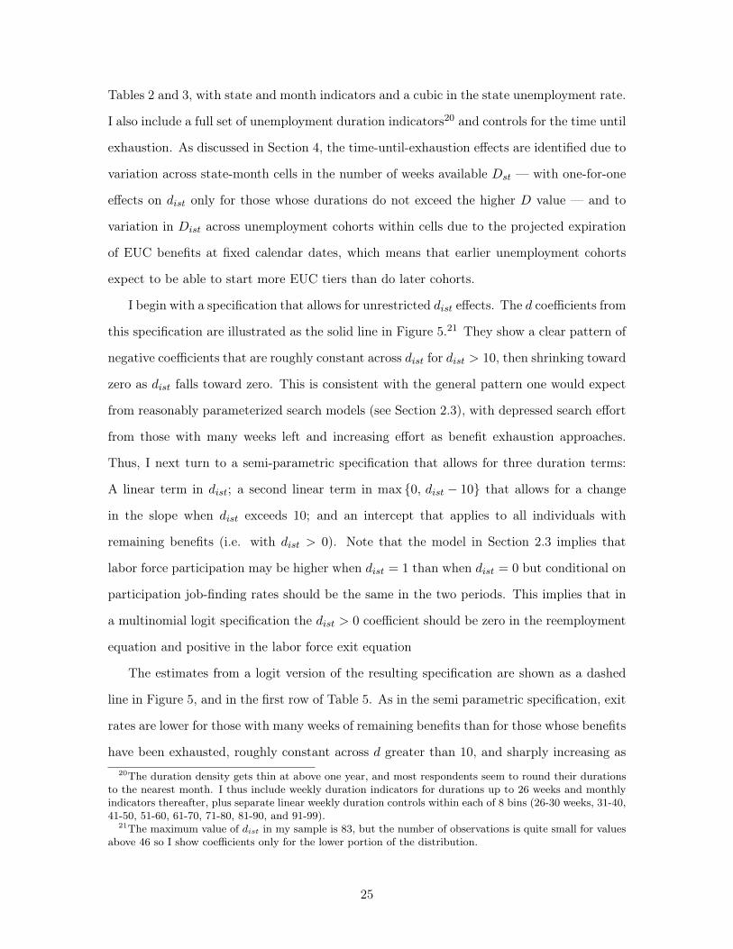
I begin with a specification that allows for unrestricted dist effects. The d coefficients from

this specification are illustrated as the solid line in Figure 5.21 They show a clear pattern of

negative coefficients that are roughly constant across dist for dist > 10, then shrinking toward

zero as dist falls toward zero. This is consistent with the general pattern one would expect

from reasonably parameterized search models (see Section 2.3), with depressed search effort

from those with many weeks left and increasing effort as benefit exhaustion approaches.

Thus, I next turn to a semi-parametric specification that allows for three duration terms:

A linear term in dist; a second linear term in max {0, dist − 10} that allows for a change

in the slope when dist exceeds 10; and an intercept that applies to all individuals with

remaining benefits (i.e. with dist > 0). Note that the model in Section 2.3 implies that

labor force participation may be higher when dist = 1 than when dist = 0 but conditional on

participation job-finding rates should be the same in the two periods. This implies that in

a multinomial logit specification the dist > 0 coefficient should be zero in the reemployment

equation and positive in the labor force exit equation

The estimates from a logit version of the resulting specification are shown as a dashed

line in Figure 5, and in the first row of Table 5. As in the semi parametric specification, exit

rates are lower for those with many weeks of remaining benefits than for those whose benefits

have been exhausted, roughly constant across d greater than 10, and sharply increasing as20The duration density gets thin at above one year, and most respondents seem to round their durations

to the nearest month. I thus include weekly duration indicators for durations up to 26 weeks and monthlyindicators thereafter, plus separate linear weekly duration controls within each of 8 bins (26-30 weeks, 31-40,41-50, 51-60, 61-70, 71-80, 81-90, and 91-99).

21The maximum value of dist in my sample is 83, but the number of observations is quite small for valuesabove 46 so I show coefficients only for the lower portion of the distribution.

25

d falls from 10 toward 0.22 There is no significant difference in exit rates between those

in their last weeks of benefits and those who have already exhausted, holding constant the

length of the spell. The rightmost column of Table 5 shows that the implied effect of UI

benefits on the UI exit rate is quite similar to those in Panel B of Table 2.

The second row of Table 5 shows a specification that includes a full set of state-by-month

indicators. This shows very similar results to those in the less restrictive specification.

In row 3, I return to the control variables from row 1, but use a multinomial logit that

distinguishes alternative types of exit from unemployment. As before, we see substantial

effects of UI benefits on both margins, though the net effects are somewhat smaller than in

Table 3. Note also the large positive coefficient for the (d > 0) indicator in the labor force

exit equation. This indicates that people in their last week of benefits are more likely to exit

the labor force than are those who have already exhausted, consistent with the idea that UI

benefits are keeping people in the labor force who would otherwise have abandoned their

searches. However, this coefficient is only marginally significant.

6 Simulations of the Effect of Unemployment Insurance Ex-

tensions

The results in Tables 2 – 5 indicate that the UI benefit extensions enacted in 2008-2010 re-

duced both the probability that a UI recipient found a job and the probability that he exited

the labor force, with somewhat larger estimated impacts on the latter than the former. But

the magnitudes are difficult to interpret. This section presents simulations of the net effect

of the extensions on labor market aggregates, obtained by comparing actual unemployment

exit hazards with counterfactual hazards that would have been observed in the absence of

UI benefit extensions.

Extrapolation of the estimated hazards to the aggregate level requires confronting an

important limitation of the longitudinally linked CPS data: The exit hazards seen in the22The increase in the exit rate as d approaches zero is consistent with the presence of a “spike” in the

exit rate at or near the exhaustion of benefits (i.e., at d = 0 or d = 1; see, e.g., Katz and Meyer, 1990a).The CPS data are not well suited to the identification of sharp spikes, however, as the monthly frequencysmooths out week-to-week changes.

26

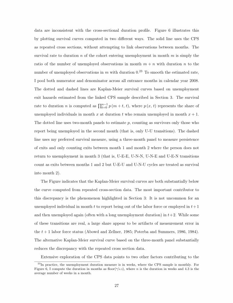
data are inconsistent with the cross-sectional duration profile. Figure 6 illustrates this

by plotting survival curves computed in two different ways. The solid line uses the CPS

as repeated cross sections, without attempting to link observations between months. The

survival rate to duration n of the cohort entering unemployment in month m is simply the

ratio of the number of unemployed observations in month m + n with duration n to the

number of unemployed observations in m with duration 0.23 To smooth the estimated rate,

I pool both numerator and denominator across all entrance months in calendar year 2008.

The dotted and dashed lines are Kaplan-Meier survival curves based on unemployment

exit hazards estimated from the linked CPS sample described in Section 3. The survival

rate to duration n is computed as�n−1

t=0 p (m+ t, t), where p (x, t) represents the share of

unemployed individuals in month x at duration t who remain unemployed in month x+ 1.

The dotted line uses two-month panels to estimate p, counting as survivors only those who

report being unemployed in the second month (that is, only U-U transitions). The dashed

line uses my preferred survival measure, using a three-month panel to measure persistence

of exits and only counting exits between month 1 and month 2 where the person does not

return to unemployment in month 3 (that is, U-E-E, U-N-N, U-N-E and U-E-N transitions

count as exits between months 1 and 2 but U-E-U and U-N-U cycles are treated as survival

into month 2).

The Figure indicates that the Kaplan-Meier survival curves are both substantially below

the curve computed from repeated cross-section data. The most important contributor to

this discrepancy is the phenomenon highlighted in Section 3: It is not uncommon for an

unemployed individual in month t to report being out of the labor force or employed in t+1

and then unemployed again (often with a long unemployment duration) in t+2. While some

of these transitions are real, a large share appear to be artifacts of measurement error in

the t+ 1 labor force status (Abowd and Zellner, 1985; Poterba and Summers, 1986, 1984).

The alternative Kaplan-Meier survival curve based on the three-month panel substantially

reduces the discrepancy with the repeated cross section data.

Extensive exploration of the CPS data points to two other factors contributing to the23In practice, the unemployment duration measure is in weeks, where the CPS sample is monthly. For

Figure 6, I compute the duration in months as floor(n/4.3), where n is the duration in weeks and 4.3 is theaverage number of weeks in a month.

27

remaining discrepancy. The first is so-called “rotation group bias”: The measured unemploy-

ment rate is higher in the first month of the CPS panel than in later months, even though

each rotation group should be a random sample from the population (see, e.g., Bailar, 1975;

Solon, 1986; Shockey, 1988). Second, individuals starting a new unemployment spell often

report long durations. This phenomenon is particularly common when the employment spell

that precedes the entry into unemployment is short, suggesting that respondents may be

conflating what appear to be distinct spells into a longer super-spell. However, this does not

seem to be a complete explanation. In 2006 and 2007, for example, there are nearly 2,400

respondents observed to be employed for three consecutive months and then unemployed

in the fourth month; 10% of these report unemployment durations in the fourth month of

longer than 6 weeks.

A full econometric model of measurement error in CPS labor force status and unemploy-

ment durations is beyond the scope of this paper. Instead, I use ad hoc procedures similar in

spirit to the “raking” algorithm that the Bureau of Labor Statistics uses in constructing the

gross flows data (Frazis et al., 2005) to force consistency between the Kaplan-Meier survival

curve and the cross-sectional duration profile. I take the view that the cross-sectional profile

is correct, and that differences between this profile and my (adjusted) Kaplan-Meier sur-

vival curve are due to “late entries” into unemployment.24 I use two different adjustments;

I argue below that one approach is likely to lead me to somewhat overstate the effect of UI

extensions while the other is likely to understate it.

Let u (m, n, s) be the count of individuals observed in month m in state s with duration

n (in months) obtained from cross-sectional data; let p (m, n, s) represent the probability

that an individual in month m in state s with duration n persists in unemployment by

month m+ 1; and let pc (m, n, s) be the counterfactual persistence probability that would

be observed in the absence of unemployment insurance extensions. Both p and pc are

obtained from fitted values from the exit regressions presented in Section 5.

The unemployed at duration n are the survivors from among the unemployed at n − 1

24Of course, it is possible that the Kaplan-Meier curve (perhaps even the unadjusted one) is correctand that the cross-sectional curve overstates survival due to misreporting of durations. However, externalevidence suggests that this is unlikely. For example, the UI system tabulates the number of individuals whoexhaust their (regular program) benefits each month; the implied exhaustion rates are much more nearlyconsistent with the cross-sectional survival curve than with the Kaplan-Meier curve.

28

one month prior. This creates a link between the u () and p () functions:

u (m, n, s) = u (m− 1, n− 1, s) p (m− 1, n− 1, s) + e (m, n, s) . (7)

In population data without measurement error, the residual e (m, n, s) would be identically

zero. The actual residual in (7) has two components. The first is mean-zero sampling error,

which may cause the number of unemployed in newly entering rotation groups to differ from

the number rotating out. The second is the “late entry” phenomenon discussed above, which

leads to E [e (m, n, s)] > 0 for most n.

We wish to compare u (m, n, s) to the counterfactual unemployment uc (m, n, s) that

would be observed had the persistence probabilities been pc rather than p. To do this,

I assume that entry into unemployment at duration 0 is not affected by UI extensions:

u (m, 0, s) = uc (m, 0, s) for all m and s. My two approaches differ in their assumptions

about the counterfactual values of e (m, n, s).

My first approach begins with an alternative expression for u (m, n, s) obtained by

recursively substituting into the right side of (7):

u (m, n, s) = u (m− n, 0, s)n−1�

t=0

p (m− n+ t, t, s) + E (m, n, s) , (8)

where E (m, n, s) ≡�n

r=1 [e (m− n+ r, r, s)�n

t=r p (m− n+ t, t, s)]. (Hereafter, I sup-

press the month and state subscripts, understanding that increments to duration require

corresponding increments to the month of observation in order to maintain a focus on the

same entry cohort.) In this approach, I assume that the cumulative count of surviving late

entries E (n) is unaffected by UI extensions. I estimate E (n) ≡ u (n) − u (0)�n−1

t=0 p (t),

then use (8) to construct a counterfactual unemployment count

uc1 (n) ≡ u (0)n−1�

t=0

pc (t) + E (n) . (9)

Note that E (n) is simply the vertical distance between the solid and long-dashed lines in

29

Figure 6, evaluated at duration n.

The second approach assumes instead that the per-period late entries e (n) are unaffected

by UI extensions but that the subsequent persistence of these late entrants is affected.

Following (7), I estimate e (d) = u (n) − u (n− 1) p (n− 1), then define the counterfactual

count iteratively as:

uc2 (n) = uc2 (n− 1) pc (n− 1) + e (n) . (10)

This can be rewritten to yield an intuitive expression for uc2 (n) in terms of actual counts

u (n) and two adjustments:

uc2 (n) ≡ u (n) + u (n− 1) [pc (n− 1)− p (n− 1)] (11)

+�uc2 (n− 1)− u (n− 1)

�pc (n− 1)

The first adjustment — the second term on the right side of (11) — reflects differences

between the actual and counterfactual scenarios in unemployment persistence at duration

n− 1, while the second adjustment — the third term in (11) — captures differences in exit

at durations t < n− 1, multiplied by the probability of surviving from n− 1 to n.

Neither assumption about the late entries is particularly plausible. First, there is no

reason to expect that the job search behavior of “late entrants” to unemployment will be

unaffected by UI extensions, particularly if these late entrants are in part an artifact of

measurement error in the pre-unemployment labor force status. If the late entrants are in

fact affected, Ec (n) < E (n) and uc1 (n) > uc (n). This implies that the UI effect inferred

from the comparison of u (n) with uc1 (n) will understate the magnitude of the effect of UI

extensions.

On the other hand, insofar as the late entrants are composed of people completing a cycle

from unemployment to non-participation and back, UI extensions that reduce the flow from

unemployment into non-participation would also likely reduce the number of subsequent

late entries. This would imply ec (n) > e (n) and uc2 (n) < uc (n), so a UI effect inferred

from the comparison of u (n) with uc2 (n) will likely overstate the magnitude of the effect of

30

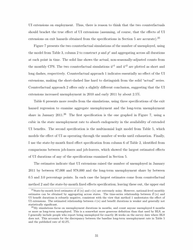
UI extensions on employment. Thus, there is reason to think that the two counterfactuals

should bracket the true effect of UI extensions (assuming, of course, that the effects of UI

extensions on exit hazards obtained from the specifications in Section 5 are accurate).25

Figure 7 presents the two counterfactual simulations of the number of unemployed, using

the model from Table 3, column 2 to construct p and pc and aggregating across all durations

at each point in time. The solid line shows the actual, non-seasonally-adjusted counts from

the monthly CPS. The two counterfactual simulations uc1 and uc2 are plotted as short and

long dashes, respectively. Counterfactual approach 1 indicates essentially no effect of the UI

extensions, making the short-dashed line hard to distinguish from the solid “actual” series.

Counterfactual approach 2 offers only a slightly different conclusion, suggesting that the UI

extensions increased unemployment in 2010 and early 2011 by about 2.5%.

Table 6 presents more results from the simulations, using three specifications of the exit

hazard regression to examine aggregate unemployment and the long-term unemployment

share in January 2011.26 The first specification is the one graphed in Figure 7, using a

cubic in the state unemployment rate to absorb endogeneity in the availability of extended

UI benefits. The second specification is the multinomial logit model from Table 5, which

models the effect of UI as operating through the number of weeks until exhaustion. Finally,

I use the state-by-month fixed effect specification from column 6 of Table 2, identified from

comparisons between job-losers and job-leavers, which showed the largest estimated effects

of UI durations of any of the specifications examined in Section 5.

The estimates indicate that UI extensions raised the number of unemployed in January

2011 by between 87,000 and 978,000 and the long-term unemployment share by between

0.5 and 3.0 percentage points. In each case the largest estimates come from counterfactual

method 2 and the state-by-month fixed effects specification; leaving these out, the upper end25State-by-month level estimates of E (n) and e (n) are extremely noisy. However, national-level monthly

estimates can be obtained by aggregating across states. The time-series relationship between E (n) andUI benefit durations is robustly negative, consistent with the view that method 1 understates the effect ofUI extensions. The estimated relationship between e (n) and benefit durations is weaker and generally notstatistically significant.

26My simulations focus on unemployment durations in months, and count anyone unemployed 6 monthsor more as long-term unemployed. This is a somewhat more generous definition than that used by BLS, asI generally include people who report being unemployed for exactly 26 weeks on the survey date where BLSdoes not. This accounts for the discrepancy between the baseline long-term unemployment rate in Table 5and the published rate of 42.2%.

31

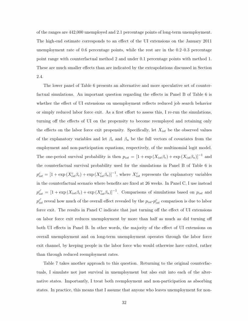
of the ranges are 442,000 unemployed and 2.1 percentage points of long-term unemployment.

The high-end estimate corresponds to an effect of the UI extensions on the January 2011

unemployment rate of 0.6 percentage points, while the rest are in the 0.2–0.3 percentage

point range with counterfactual method 2 and under 0.1 percentage points with method 1.

These are much smaller effects than are indicated by the extrapolations discussed in Section

2.4.

The lower panel of Table 6 presents an alternative and more speculative set of counter-

factual simulations. An important question regarding the effects in Panel B of Table 6 is

whether the effect of UI extensions on unemployment reflects reduced job search behavior

or simply reduced labor force exit. As a first effort to assess this, I re-run the simulations,

turning off the effects of UI on the propensity to become reemployed and retaining only

the effects on the labor force exit propensity. Specifically, let Xist be the observed values

of the explanatory variables and let βe and βn be the full vectors of covariates from the

employment and non-participation equations, respectively, of the multinomial logit model.

The one-period survival probability is then pist = [1 + exp (Xistβe) + exp (Xistβn)]−1 and

the counterfactual survival probability used for the simulations in Panel B of Table 6 is

pcist = [1 + exp (Xcistβe) + exp (Xc

istβn)]−1, where Xc

ist represents the explanatory variables

in the counterfactual scenario where benefits are fixed at 26 weeks. In Panel C, I use instead

pc�ist = [1 + exp (Xistβe) + exp (Xc

istβn)]−1. Comparisons of simulations based on pist and

pc�ist reveal how much of the overall effect revealed by the pist-pcist comparison is due to labor

force exit. The results in Panel C indicate that just turning off the effect of UI extensions

on labor force exit reduces unemployment by more than half as much as did turning off

both UI effects in Panel B. In other words, the majority of the effect of UI extensions on

overall unemployment and on long-term unemployment operates through the labor force

exit channel, by keeping people in the labor force who would otherwise have exited, rather

than through reduced reemployment rates.

Table 7 takes another approach to this question. Returning to the original counterfac-

tuals, I simulate not just survival in unemployment but also exit into each of the alter-

native states. Importantly, I treat both reemployment and non-participation as absorbing

states. In practice, this means that I assume that anyone who leaves unemployment for non-

32

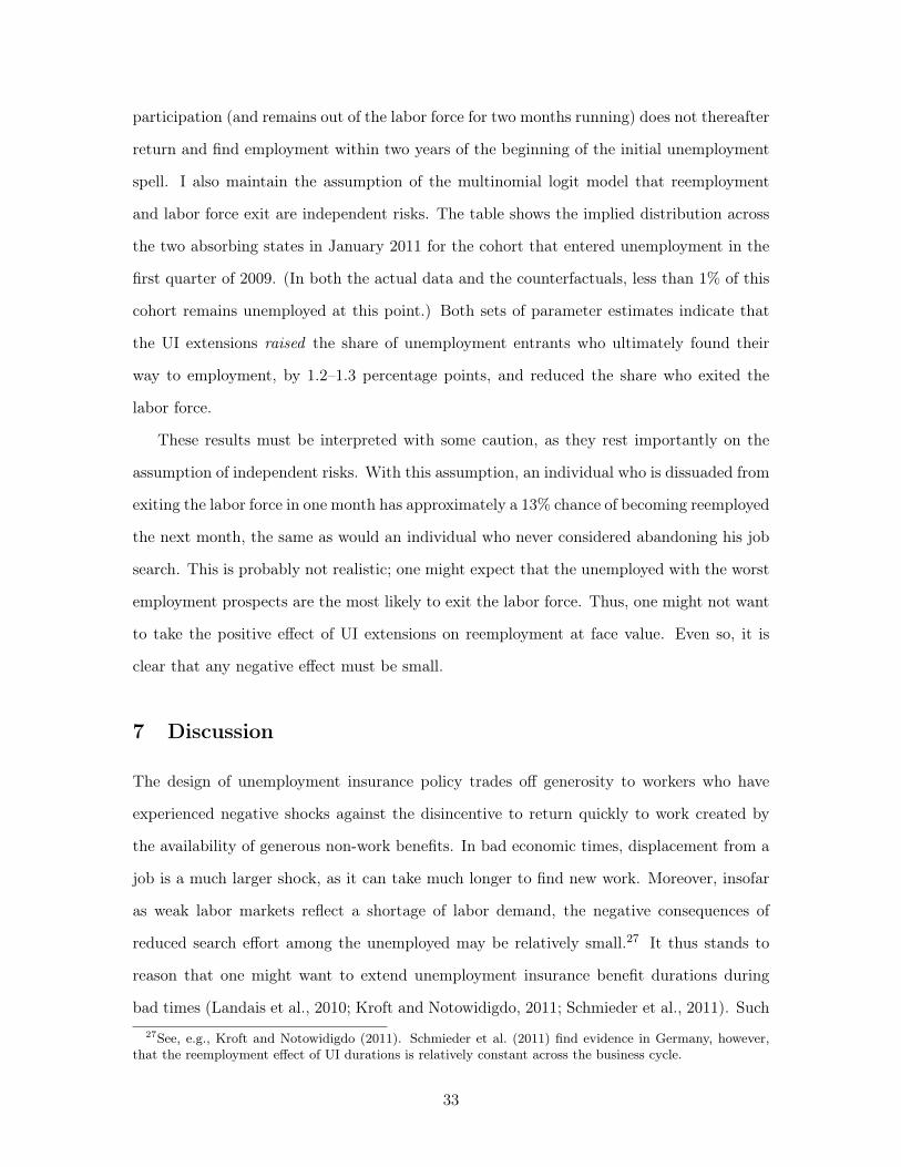
participation (and remains out of the labor force for two months running) does not thereafter

return and find employment within two years of the beginning of the initial unemployment

spell. I also maintain the assumption of the multinomial logit model that reemployment

and labor force exit are independent risks. The table shows the implied distribution across

the two absorbing states in January 2011 for the cohort that entered unemployment in the

first quarter of 2009. (In both the actual data and the counterfactuals, less than 1% of this

cohort remains unemployed at this point.) Both sets of parameter estimates indicate that

the UI extensions raised the share of unemployment entrants who ultimately found their

way to employment, by 1.2–1.3 percentage points, and reduced the share who exited the

labor force.

These results must be interpreted with some caution, as they rest importantly on the

assumption of independent risks. With this assumption, an individual who is dissuaded from

exiting the labor force in one month has approximately a 13% chance of becoming reemployed

the next month, the same as would an individual who never considered abandoning his job

search. This is probably not realistic; one might expect that the unemployed with the worst

employment prospects are the most likely to exit the labor force. Thus, one might not want

to take the positive effect of UI extensions on reemployment at face value. Even so, it is

clear that any negative effect must be small.

7 Discussion

The design of unemployment insurance policy trades off generosity to workers who have

experienced negative shocks against the disincentive to return quickly to work created by

the availability of generous non-work benefits. In bad economic times, displacement from a

job is a much larger shock, as it can take much longer to find new work. Moreover, insofar

as weak labor markets reflect a shortage of labor demand, the negative consequences of

reduced search effort among the unemployed may be relatively small.27 It thus stands to

reason that one might want to extend unemployment insurance benefit durations during

bad times (Landais et al., 2010; Kroft and Notowidigdo, 2011; Schmieder et al., 2011). Such27See, e.g., Kroft and Notowidigdo (2011). Schmieder et al. (2011) find evidence in Germany, however,

that the reemployment effect of UI durations is relatively constant across the business cycle.

33

extensions can have macroeconomic benefits as well, as the unemployed likely have a high

marginal propensity to consume and UI payments thus have relatively large multipliers

(Congressional Budget Office, 2010).

However, the advisability of long UI extensions depends importantly on the view that

the reduced job search induced by these extensions will not overly slow the labor market

matching process. Many commentators have argued that the 99 weeks of benefits available

through the EUC and EB programs in 2010 and 2011 have gone too far, some pointing to

the apparent outward shift of the Beveridge Curve in 2010 (Elsby et al., 2010) as evidence

that UI extensions have reduced labor supply sufficiently to noticeably slow the recovery of

the labor market.

It is ultimately an empirical question whether UI extensions lead to large reductions

in job finding. But the effect of extensions on job finding rates is hard to identify, because

extensions are usually implemented in response to poor labor market conditions. Fortunately

for the researcher (if not for UI recipients themselves), the haphazard way that the EUC

program was gradually expanded and then repeatedly renewed generates a great deal of

variation in benefit availability that is plausibly exogenous to the demand conditions that

otherwise confound efforts to estimate the benefit duration effect.

Using a variety of comparisons that isolate different components of the variation in

benefit availability, I find that extended benefits do reduce the rate at which unemployed

workers reenter employment. But the reductions are small, in most specifications smaller

than effects of extended benefits on labor force exit and always much smaller than what one

would have expected based on older estimates in the literature. The two effects both lead to

increases in measured unemployment, but combined they have raised the unemployment rate

by only about 0.3 percentage points, implying that the vast majority of the increase in the

unemployment rate was due to demand shocks rather than to UI-induced supply reductions.

Moreover, less than half of the small UI effect comes from reduced reemployment rather

than from reduced non-participation (i.e., from increased labor supply). Some simulations

even suggest that the availability of extended benefits might have raised reemployment rates

of displaced workers, by keeping them from abandoning their searches prematurely.

Any negative effects of the recent unemployment insurance extensions on job search are

34

clearly quite small, too small to outweigh the benefits of transfers to people who have been

out of work for over a year in conditions where job-finding prospects are bleak (Gruber,

1997). Moreover, all of the estimates herein are partial equilibrium; I do not account for

congestion on the supply side of the labor market. Incorporating these spillovers would make

extensions more attractive, as reduced job search among a subset of the unemployed would

not translate one-for-one into reduced employment but would rather simply shift jobs from

the UI recipients to other job seekers, particularly at times when jobs are rationed (Landais

et al., 2010). The evidence here thus supports the view that optimal UI program design

would provide for generous extensions of benefit durations in deep recessions that last until

the labor market is strong enough to give displaced workers a realistic chance of finding new

employment before their benefits expire.

References

Aaronson, Daniel, Bhashkar Mazumder, and Shani Schechter, “What is behindthe rise in long-term unemployment?,” Economic Perspectives (Federal Reserve Bank ofChicago), 2nd Quarter 2010, 34 (2).

Abowd, John M. and Arnold Zellner, “Estimating gross labor-force flows,” Journal ofBusiness & Economic Statistics, 1985, 3 (3), 254–283.

Anderson, Patricia M. and Bruce D. Meyer, “Unemployment Insurance takeup ratesand the after-tax value of benefits,” Quarterly Journal of Economics, 1997, 112 (3), 913–937.

Bailar, Barbara A., “The effects of rotation group bias on estimates from panel surveys,”Journal of the American Statistical Association, 1975, 70 (349), 23–30.

Barro, Robert, “The folly of subsidizing unemployment,” Wall Street Journal, August 302010, August 30.

Card, David and Philip B. Levine, “Extended benefits and the duration of UI spells:Evidence from the New Jersey extended benefit program,” Journal of Public Economics,2000, 78 (1-2), 107–138.

, Raj Chetty, and Andrea Weber, “Cash-on-hand and competing models of intertem-poral behavior: New evidence from the labor market,” Quarterly Journal of Economics,2007, 122 (4), 1511–1560.

, , and , “The spike at benefit exhaustion: Leaving the unemployment system orstarting a new job?,” The American Economic Review, 2007, 97 (2), 113–118.

35

Chetty, Raj, “Moral hazard vs. liquidity and optimal unemployment insurance,” Journalof Political Economy, 2008, 116 (2), 173–234.

Congressional Budget Office, “Policies for increasing economic growth and employmentin 2010 and 2011,” Publication 4077 January 2010.

Duggan, Mark and Scott Imberman, “Why are the DI rolls skyrocketing? The contri-bution of population characteristics, program changes, and economic conditions,” in DavidCutler and David Wise, eds., Health at Older Ages, Chicago, IL: University of ChicagoPress, 2009.

Elsby, Michael W, Bart Hobijn, and Aysegul Sahin, “The labor market in the GreatRecession,” Brookings Papers on Economic Activity, 2010, Spring.

Farber, Henry S. and Robert Valletta, “Extended unemployment insurance and un-employment duration in the Great Recession: The U.S. experience,” manuscript June 242011.

Federal-State Extended Unemployment Compensation Act of 1970, http://workforcesecurity.doleta.gov/unemploy/EB_law_for_web.pdf. Accessed June 28,2011. Undated.

Frazis, Harley J., Edwin L. Robison, Thomas D. Evans, and Martha A. Duff, “Es-timating gross flows consistent with stocks in the CPS,” Monthly Labor Review, September2005, 128 (9), 3–9.

Frey, William H., “The great American migration slowdown: Regional and metropolitandimensions,” Technical Report, The Brookings Institution December 2009.

Fujita, Shigeru, “Economic effects of the unemployment insurance benefit,” Business Re-view (Federal Reserve Bank of Philadelphia), Fourth Quarter 2010.

, “Effects of extended unemployment insurance benefits: Evidence from the monthly CPS,”Working paper 10-35/R, Federal Reserve Bank of Philadelphia January 2011.

Grubb, David, “Assessing the impact of recent unemployment insurance extensions in theUnited States,” Working paper, OECD May 25 2011.

Gruber, Jonathan, “The consumption smoothing benefits of unemployment insurance,”American Economic Review, March 1997, 87 (1), 192–205.

Howell, David R. and Bert M. Azizoglu, “Unemployment benefits and work incentives:The U.S. labor market in the Great Recession,” Working Paper 257, Political EconomyResearch Institute, University of Massachusetts Amherst May 2011.

Joint Economic Committee, “Extending unemployment insurance benefits: The cost ofinaction for disabled workers,” Report May 2010.

Kaplan, Greg and Sam Schulhofer-Wohl, “Interstate migration has fallen less thanyou think: Consequences of hot deck imputation in the Current Population Survey,” StaffReport 458, Federal Reserve Bank of Minneapolis June 2011.

Katz, Lawrence, “Layoffs, recall, and the duration of unemployment,” Working paper1825, National Bureau of Economic Research January 1986.

36

Katz, Lawrence F. and Bruce D. Meyer, “The impact of the potential duration ofunemployment benefits on the duration of unemployment,” Journal of Public Economics,1990, 41 (1), 45–72.

and , “Unemployment Insurance, recall expectations, and unemployment outcomes,”The Quarterly Journal of Economics, November 1990, 105 (4), 973–1002.

Kroft, Kory and Matthew J. Notowidigdo, “Should unemployment insurance vary withthe unemployment rate? Theory and evidence,” working paper 17173, National Bureauof Economic Research June 2011.

Landais, Camille, Pascal Michaillat, and Emmanuel Saez, “Optimal unemploymentinsurance over the business cycle,” working paper 16526, National Bureau of EconomicResearch November 2010.

Mazumder, Bhashkar, “How did unemployment insurance extensions affect the unem-ployment rate in 2008-10?,” Chicago Fed Letter, April 2011, 285.

National Employment Law Project, “Q&A: The basics of the Extended Benefits pro-gram,” Fact Sheet February 3 2011.

Poterba, James M. and Lawrence H. Summers, “Response variation in the CPS:Caveats for the unemployment analyst,” Monthly Labor Review, 1984, 107 (3), 37–43.

and , “Reporting errors and labor market dynamics,” Econometrica, November 1986,54 (6), 1319–1338.

and , “Unemployment benefits and labor market transitions: A multinomial logitmodel with errors in classification,” The Review of Economics and Statistics, May 1995,77 (2), 207–216.

Schmieder, Johannes F., Till von Wachter, and Stefan Bender, “The effects ofextended unemployment insurance over the business cycle: Evidence from regression dis-continuity estimates over twenty years,” Working paper March 2011.

Shockey, James W., “Adjusting for response error in panel surveys,” Sociological Methods& Research, 1988, 17 (1), 65.

Sider, Hal, “Unemployment duration and incidence: 1968-82,” The American EconomicReview, June 1985, 75 (3), 461–472.

Solon, Gary, “Labor Supply Effects of Extended Unemployment Benefits,” The Journal ofHuman Resources, Spring 1979, 14 (2), 247–255.

, “Effets of rotation group bias on estimation of unemployment,” Journal of Business andEconomic Statistics, January 1986, 4, 105–109.

Valetta, Rob and Katherine Kuang, “Extended unemployment and UI benefits,”FRBSF Economic Letter, April 2010, 2010 (12).

37

Appendix: Proofs of propositions

All proofs are by induction.

Proof of Proposition 1. First, note that ∂VU (s, 0)∂s = ∂VU (s, 1)

∂s for all s. Thus, s∗1 = s∗0 andVU (1)− VU (0) = u (b)− u (0) > 0. Second, assume VU (x) > VU (x− 1) for some x. Then

VU (x+ 1)− VU (x) = VU�s∗x+1, x+ 1

�− VU (s∗x, x)

≥ VU (s∗x, x+ 1)− VU (s∗x, x)

= δ (VU (x)− VU (x− 1)) (1− p (s∗x)) > 0. (12)

Note that the inequality here follows from the definition of s∗x+1 ≡ argmaxVU (s, x+ 1).

Proof of Proposition 2. See above for s∗1 = s∗0. For d ≥ 1, s∗d is defined by p� (s∗d) =1

δ(VE−VU (d−1)) . Proposition 1 thus implies that p��s∗d+1

�< p� (s∗d), so p�� (s) < 0 implies

s∗d+1 > s∗d.

Proof of Proposition 3. Let s∗∗d = argmax VU (s, d) and let ηd = 1 (s∗∗d ≥ θ). I show thatηd+1 = ηd for all d > 0.

Begin by considering the case where η0 = 1 and s∗∗0 > θ. Then an argument identical tothat above implies that the search requirement is never binding: s∗∗1 = s∗∗0 and for all x > 0,VU (x+ 1)− V (x) > 0, s∗∗x+1 > s∗∗x and ηx = 1.

Next, suppose that ηd = 0 for some d ≥ 1, but ηd+1 = 1. Without loss of generality,assume that ηx = 0 for all 0 ≤ x ≤ d. (This merely means that we have chosen the smallestd such that ηd+1 = 1.) This implies that

VU (x) = maxs<θ

u (0)− s+ δ�p (s)VE +

�1− p (s) VU (x)

��

= maxs<θ

u (0)− s+ δp (s)VE

1− δ (1− p (s))(13)

for all 0 ≤ x ≤ d. Note that the right-hand side of (13) does not vary with x, so the leftside does not either. In particular, VU (d) = VU (d− 1). Moreover, because labor force exitwith sd+1 = s∗d < θ is a feasible option with d+1 weeks of benefits available, it must be thecase that VU (d+ 1) > VU (d). Next, note that

VU (d) < VU (d+ 1)

= VU�s∗∗d+1, d+ 1

�

= u (b)− s∗∗d+1 + δ�p�s∗∗d+1

�VE +

�1− p

�s∗∗d+1

�VU (d)

��

= VU�s∗∗d+1, d

�+ δ

�1− p

�s∗∗d+1

�� �VU (d)− VU (d− 1)

�

< VU (d) + δ�1− p

�s∗∗d+1

�� �VU (d)− VU (d− 1)

�, (14)

where the final inequality follows from a revealed preference argument for benefit durationd. This implies that VU (d) > VU (d− 1), a contradiction.

There are thus only three possible values for the ηd sequence: ηd = 1 for all d ≥ 0; ηd = 0

for all d ≥ 0, or ηd =

�0 if d = 0

1 if d > 0. Unemployment to non-participation transitions thus

38

occur only when benefits are exhausted; benefit extensions will delay these transitions forthose who would otherwise have exhausted their benefits.

39

! "#!

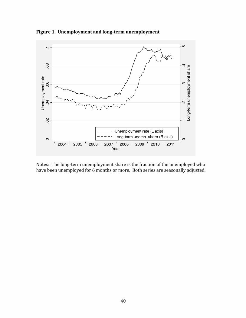
!"#$%&'()''*+&,-./0,&+1'2+3'./+#41&%,'$+&,-./0,&+1''

!!

$%&'()!!*+'!,%-./&'01!2-'13,%41'-&!(+50'!6(!&+'!7058&6%-!%7!&+'!2-'13,%4'9!:+%!

+5;'!<''-!2-'13,%4'9!7%0!=!1%-&+(!%0!1%0'>!!?%&+!('06'(!50'!('5(%-5,,4!59@2(&'9>!

!

! "A!

!"#$%&'56)''7/+18.0'9./:;'/$1'/9'</=;'!

!!

$%&'()!B26&(!5-9!,54%77(C96(8+50.'(!8%1'!70%1!&+'!DEF*G!95&5H!:+68+!9'06;'!70%1!

'13,%4'0!(20;'4(>!!I13,%41'-&/&%/2-'13,%41'-&!JI/KL!7,%:(!50'!&5M'-!70%1!&+'!

0'('508+!('06'(!%-!,5<%0!7%08'!(&5&2(!7,%:(!8%-(&028&'9!<4!&+'!?20'52!%7!F5<%0!

G&5&6(&68(!70%1!,%-.6&296-5,,4!,6-M'9!1%-&+,4!NOG!76,'(>!P,,!('06'(!50'!('5(%-5,,4!

59@2(&'9!5-9!(1%%&+'9!:6&+!5!Q/1%-&+!(411'&068!&065-.2,50!1%;6-.!5;'05.'H!4&(1!R!

J4&/A!S!T4&!S!4&SALC">!

!

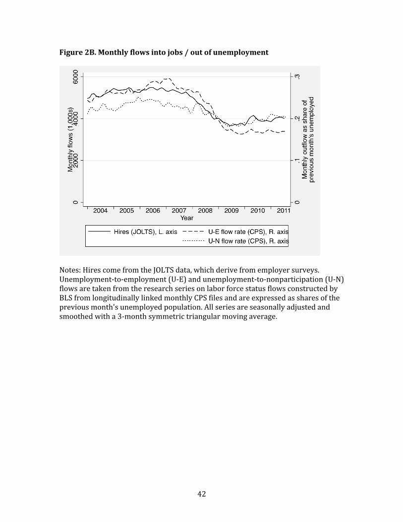
! "T!

!"#$%&'5>)'7/+18.0'9./:;'"+1/'</=;'?'/$1'/9'$+&,-./0,&+1''

!!

$%&'()!U60'(!8%1'!70%1!&+'!DEF*G!95&5H!:+68+!9'06;'!70%1!'13,%4'0!(20;'4(>!!

K-'13,%41'-&/&%/'13,%41'-&!JK/IL!5-9!2-'13,%41'-&/&%/-%-350&68635&6%-!JK/$L!

7,%:(!50'!&5M'-!70%1!&+'!0'('508+!('06'(!%-!,5<%0!7%08'!(&5&2(!7,%:(!8%-(&028&'9!<4!

?FG!70%1!,%-.6&296-5,,4!,6-M'9!1%-&+,4!NOG!76,'(!5-9!50'!'V30'(('9!5(!(+50'(!%7!&+'!

30';6%2(!1%-&+W(!2-'13,%4'9!3%32,5&6%->!P,,!('06'(!50'!('5(%-5,,4!59@2(&'9!5-9!

(1%%&+'9!:6&+!5!Q/1%-&+!(411'&068!&065-.2,50!1%;6-.!5;'05.'>!

!

! "Q!

!"#$%&'@)'*A'=&+&9"1'3$%21"/+;B';121$1/%0'2+3'2;'-&%C&"D&3'=0'%&C"-"&+1;'!

!!

$%&'()!IV3'8&5&6%-(!50'!&+%('!%7!0'8636'-&(!:+%!9%!-%&!5-&68635&'!720&+'0!,'.6(,5&6;'!

8+5-.'(!J6-8,296-.!'V&'-(6%-(!%7!&+'!IKN!30%.051L!%0!(&5&'!&06..'0!';'-&(>!!

XY5V6121!(&5&'Z!6(!&+'!(&5&'!:6&+!&+'!+6.+'(&!;5,2'!6-!5!.6;'-!1%-&+>!!XP;'05.'!

(&5&'Z!6(!&+'!2-:'6.+&'9!1'5-!580%((!(&5&'(>!

!

! ""!

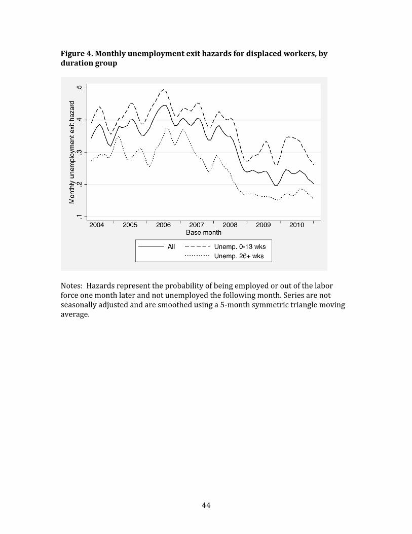
!"#$%&'E)'7/+18.0'$+&,-./0,&+1'&F"1'82G2%3;'9/%'3";-.2C&3':/%H&%;B'=0'3$%21"/+'#%/$-'!

!!

$%&'()!!U5[509(!0'30'('-&!&+'!30%<5<6,6&4!%7!<'6-.!'13,%4'9!%0!%2&!%7!&+'!,5<%0!

7%08'!%-'!1%-&+!,5&'0!5-9!-%&!2-'13,%4'9!&+'!7%,,%:6-.!1%-&+>!G'06'(!50'!-%&!

('5(%-5,,4!59@2(&'9!5-9!50'!(1%%&+'9!2(6-.!5!\/1%-&+!(411'&068!&065-.,'!1%;6-.!

5;'05.'>!

!

! "\!

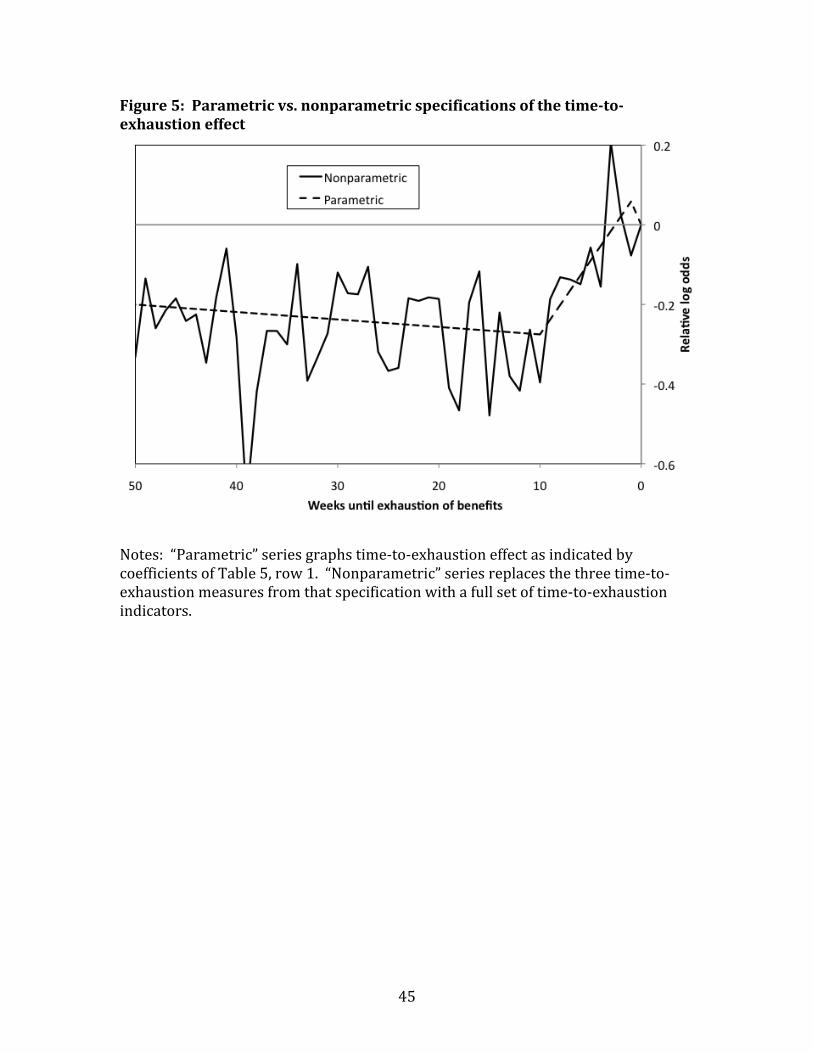
!"#$%&'IJ''K2%2,&1%"C'D;)'+/+-2%2,&1%"C';-&C"9"C21"/+;'/9'18&'1",&41/4&F82$;1"/+'&99&C1'

!

$%&'()!!XO5051'&068Z!('06'(!.053+(!&61'/&%/'V+52(&6%-!'77'8&!5(!6-9685&'9!<4!

8%'77686'-&(!%7!*5<,'!\H!0%:!A>!!X$%-35051'&068Z!('06'(!0'3,58'(!&+'!&+0''!&61'/&%/

'V+52(&6%-!1'5(20'(!70%1!&+5&!(3'867685&6%-!:6&+!5!72,,!('&!%7!&61'/&%/'V+52(&6%-!

6-9685&%0(>!

! "=!

!"#$%&'LJ''6.1&%+21"D&';$%D"D2.'C$%D&;'9%/,'C%/;;4;&C1"/+2.'2+3'./+#"1$3"+2..04."+H&3'3212)'!

!!

$%&'()!!]6.20'!0'7'0(!&%!2-'13,%41'-&!(3',,(!<'.6--6-.!6-!T##^>!N0%((/('8&6%-5,!

(20;6;5,!820;'!6(!8%132&'9!5(!&+'!-21<'0!2-'13,%4'9!9!1%-&+(!6-!1%-&+!1S9!

96;69'9!<4!&+'!-21<'0!2-'13,%4'9!#!1%-&+(!6-!1%-&+!1>!!_53,5-/Y'6'0!(20;6;5,!

820;'(!50'!&+'!30%928&!70%1!&R#!&%!9/A!%7!&+'!(+50'!%7!&+%('!2-'13,%4'9!6-!1%-&+!

1S&!:6&+!9205&6%-!&!:+%!0'156-!2-'13,%4'9!6-!1%-&+!1S&SAH!8%132&'9!70%1!

,%-.6&296-5,,4!,6-M'9!95&5>!!*+'!X3'0(6(&'-&!'V6&(Z!('06'(!8%2-&(!(%1'%-'!5(!

0'156-6-.!2-'13,%4'9!6-!1S&SA!67!(+'!6(!2-'13,%4'9!6-!1S&STH!0'.509,'((!%7!+'0!

1'5(20'9!(&5&2(!6-!1S&SA>!

!

! "`!

!"#$%&'M)'6C1$2.'$+&,-./0,&+1'2+3'C/$+1&%92C1$2.';",$.21"/+;':"18/$1'*A'&F1&+;"/+;'!

!!

$%&'()!!N%2-&'0758&25,!(612,5&6%-(!50'!<5('9!%-!&+'!(3'867685&6%-!6-!*5<,'!QH!N%,21-!

T>!!G''!&'V&!7%0!9'&56,(>!

!

! "^!

N2=.&'()''O$,,2%0';121";1"C;'!

!!

$%&'()!!XP,,!2-'13,%4'9Z!50'!2-'13,%4'9!%<('0;5&6%-(!70%1!&+'!Y54!T##"!a!

D5-2504!T#AA!NOG!(513,'(!:6&+!1%-&+/6-/(513,'!AH!TH!\H!%0!=>!!P,,!(&5&6(&68(!2('!NOG!

:'6.+&(>!!G2<(513,'!6-!8%,21-(!Q/"!'V8,29'(!%<('0;5&6%-(!:6&+!16((6-.!%0!5,,%85&'9!

,5<%0!7%08'!(&5&2(!6-!'6&+'0!%7!&+'!&:%!7%,,%:6-.!6-&'0;6':(H!%0!:6&+!5,,%85&'9!

2-'13,%41'-&!9205&6%-!6-!&+'!<5('!1%-&+>!

!

Job losers

Job leavers / entrants / reentrants

Job losers

Job leavers / entrants / reentrants

(1) (2) (3) (4)N 95,485 77,913 77,815 61,118Share matched to one follow-up interview 91% 91% 100% 100%Share matched to two follow-up interviews 85% 83% 100% 100%Unemployment duration (spells in progress)

Average (weeks) 22.7 21.8 23.1 22.2Share 0-13 weeks 54% 59% 54% 59%Share 14-26 weeks 17% 15% 17% 15%Share 27-98 weeks 23% 20% 24% 20%Share 99+ weeks 5% 6% 5% 6%

Share exiting unemployment by next monthCounting all exits (1+ follow-ups)

Total 39% 52% 38% 51%To employment 23% 20% 23% 20%Out of labor force 15% 32% 15% 31%

Not counting U-N-U or U-E-U transitions (2+ follow-ups)Total 30% 42% 29% 41%To employment 20% 18% 20% 18%Out of labor force 10% 24% 10% 24%

Number of weeks of unemployment benefitsStatutory 53.6 -- 54.0 --Expected (total) 43.9 -- 44.2 --Expected (remaining) 24.1 -- 24.0 --

State unemployment rate 7.7% 6.9% 7.7% 6.9%

All unemployed Subsample with 2+ follow-up interviews

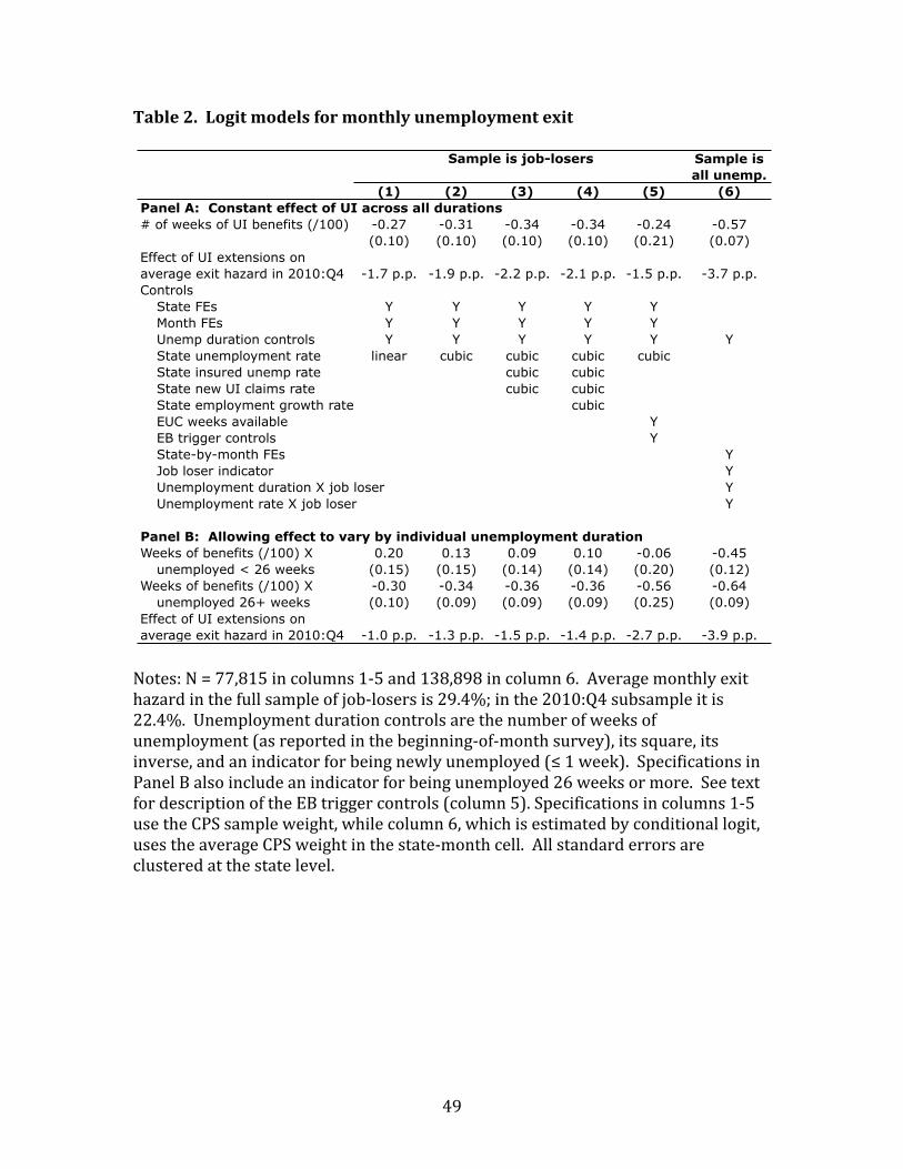
! "b!

N2=.&'5)''P/#"1',/3&.;'9/%',/+18.0'$+&,-./0,&+1'&F"1'!

!!

$%&'()!$!R!``H^A\!6-!8%,21-(!A/\!5-9!AQ^H^b^!6-!8%,21-!=>!!P;'05.'!1%-&+,4!'V6&!

+5[509!6-!&+'!72,,!(513,'!%7!@%</,%('0(!6(!Tb>"cd!6-!&+'!T#A#)B"!(2<(513,'!6&!6(!

TT>"c>!!K-'13,%41'-&!9205&6%-!8%-&0%,(!50'!&+'!-21<'0!%7!:''M(!%7!

2-'13,%41'-&!J5(!0'3%0&'9!6-!&+'!<'.6--6-./%7/1%-&+!(20;'4LH!6&(!(e250'H!6&(!

6-;'0('H!5-9!5-!6-9685&%0!7%0!<'6-.!-':,4!2-'13,%4'9!Jf!A!:''ML>!!G3'867685&6%-(!6-!

O5-',!?!5,(%!6-8,29'!5-!6-9685&%0!7%0!<'6-.!2-'13,%4'9!T=!:''M(!%0!1%0'>!!G''!&'V&!

7%0!9'(8063&6%-!%7!&+'!I?!&06..'0!8%-&0%,(!J8%,21-!\L>!G3'867685&6%-(!6-!8%,21-(!A/\!

2('!&+'!NOG!(513,'!:'6.+&H!:+6,'!8%,21-!=H!:+68+!6(!'(&615&'9!<4!8%-96&6%-5,!,%.6&H!

2('(!&+'!5;'05.'!NOG!:'6.+&!6-!&+'!(&5&'/1%-&+!8',,>!!P,,!(&5-9509!'00%0(!50'!

8,2(&'0'9!5&!&+'!(&5&'!,';',>!

!

Sample is all unemp.

(1) (2) (3) (4) (5) (6)Panel A: Constant effect of UI across all durations# of weeks of UI benefits (/100) -0.27 -0.31 -0.34 -0.34 -0.24 -0.57

(0.10) (0.10) (0.10) (0.10) (0.21) (0.07)

-1.7 p.p. -1.9 p.p. -2.2 p.p. -2.1 p.p. -1.5 p.p. -3.7 p.p.Controls

State FEs Y Y Y Y YMonth FEs Y Y Y Y YUnemp duration controls Y Y Y Y Y YState unemployment rate linear cubic cubic cubic cubicState insured unemp rate cubic cubicState new UI claims rate cubic cubicState employment growth rate cubicEUC weeks available YEB trigger controls YState-by-month FEs YJob loser indicator YUnemployment duration X job loser YUnemployment rate X job loser Y

Panel B: Allowing effect to vary by individual unemployment durationWeeks of benefits (/100) X 0.20 0.13 0.09 0.10 -0.06 -0.45

unemployed < 26 weeks (0.15) (0.15) (0.14) (0.14) (0.20) (0.12)Weeks of benefits (/100) X -0.30 -0.34 -0.36 -0.36 -0.56 -0.64

unemployed 26+ weeks (0.10) (0.09) (0.09) (0.09) (0.25) (0.09)

-1.0 p.p. -1.3 p.p. -1.5 p.p. -1.4 p.p. -2.7 p.p. -3.9 p.p.

Sample is job-losers

Effect of UI extensions on average exit hazard in 2010:Q4

Effect of UI extensions on average exit hazard in 2010:Q4

! \#!

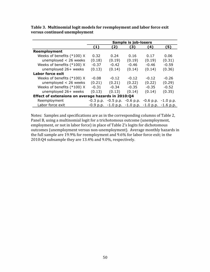
N2=.&'@)''7$.1"+/,"2.'./#"1',/3&.;'9/%'%&&,-./0,&+1'2+3'.2=/%'9/%C&'&F"1'D&%;$;'C/+1"+$&3'$+&,-./0,&+1''

!!

$%&'()!!G513,'(!5-9!(3'867685&6%-(!50'!5(!6-!&+'!8%00'(3%-96-.!8%,21-(!%7!*5<,'!TH!

O5-',!?H!2(6-.!5!12,&6-%165,!,%.6&!7%0!5!&068+%&%1%2(!%2&8%1'!J2-'13,%41'-&H!

'13,%41'-&H!%0!-%&!6-!,5<%0!7%08'L!6-!3,58'!%7!*5<,'!Tg(!,%.6&(!7%0!968+%&%1%2(!

%2&8%1'(!J2-'13,%41'-&!;'0(2(!-%-/2-'13,%41'-&L>!!P;'05.'!1%-&+,4!+5[509(!6-!

&+'!72,,!(513,'!50'!Ab>bc!7%0!0''13,%41'-&!5-9!b>=c!7%0!,5<%0!7%08'!'V6&d!6-!&+'!

T#A#)B"!(2<(513,'!&+'4!50'!AQ>"c!5-9!b>#cH!0'(3'8&6;',4>!

!

(1) (2) (3) (4) (5)Reemployment

Weeks of benefits (*100) X 0.32 0.24 0.16 0.17 0.06unemployed < 26 weeks (0.18) (0.19) (0.19) (0.19) (0.31)

Weeks of benefits (*100) X -0.37 -0.42 -0.46 -0.46 -0.59unemployed 26+ weeks (0.13) (0.14) (0.14) (0.14) (0.36)

Labor force exitWeeks of benefits (*100) X -0.08 -0.12 -0.12 -0.12 -0.26

unemployed < 26 weeks (0.21) (0.21) (0.22) (0.22) (0.29)Weeks of benefits (*100) X -0.31 -0.34 -0.35 -0.35 -0.52

unemployed 26+ weeks (0.13) (0.13) (0.14) (0.14) (0.35)Effect of extensions on average hazards in 2010:Q4

Reemployment -0.3 p.p. -0.5 p.p. -0.6 p.p. -0.6 p.p. -1.0 p.p.Labor force exit -0.9 p.p. -1.0 p.p. -1.0 p.p. -1.0 p.p. -1.6 p.p.

Sample is job-losers

! \A!

N2=.&'E)''6.1&%+21"D&';-&C"9"C21"/+;''

'!

$%&'()!?5(',6-'!(3'867685&6%-!6-!0%:!A!6(!&+5&!70%1!8%,21-!T!%7!*5<,'!Q>!!h%:!T!599(!

8%-&0%,(!7%0!.'-9'0H!1506&5,!(&5&2(H!.'-9'0i15006'9H!76;'!5.'!.0%23(H!&+0''!'9285&6%-!

85&'.%06'(H!5-9!AT!30'/96(3,58'1'-&!6-92(&06'(>!!h%:!Q!599(!5-!6-9685&%0!7%0!

9205&6%-(!%7!'V58&,4!T=!:''M(!5-9!6&(!6-&'058&6%-!:6&+!-21<'0!%7!:''M(!%7!Kj!

<'-'76&(!5;56,5<,'>!h%:!"!90%3(!%<('0;5&6%-(!:+%('!2-'13,%41'-&!9205&6%-!5&!&+'!

<'.6--6-.!%7!&+'!(3',,!%0!&+'!760(&!NOG!6-&'0;6':!:5(!T=H!\TH!%0!`^!:''M(>!!h%:!\!

8%2-&(!5,,!K/$!5-9!K/I!&05-(6&6%-(!5(!'V6&(!70%1!2-'13,%41'-&H!';'-!&+%('!J&+'!K/

$/K!5-9!K/I/K!&05-(6&6%-(L!&+5&!0'&20-!&%!2-'13,%41'-&!&+'!7%,,%:6-.!1%-&+>!h%:(!

"/`!2('!&+'!<5(',6-'!(3'867685&6%-!%-!9677'0'-&!(2<(513,'(d!&+'!+5[509(!8%00'(3%-9!

&%!5;'05.'!+5[509(!7%0!&+'!(2<(513,'(>!

!

Avg. hazard in 2010:Q4

Effect of UI extensions

Avg. hazard in 2010:Q4

Effect of UI extensions

(1) (2) (3) (4)(1) Baseline 13.4% -0.5 p.p. 9.0% -1.0 p.p.(2) Add indiv. covariates 13.4% -0.5 p.p. 9.0% -1.2 p.p.(3) Separate effect on 26 wks 13.4% -0.5 p.p. 9.0% -1.0 p.p.(4) Drop round number

durations 12.8% -0.5 p.p. 7.9% -1.5 p.p.(5) Count all UE exits 16.5% -0.6 p.p. 13.7% -1.3 p.p.Subsamples(6) Age 25-54 14.1% -1.1 p.p. 7.5% -1.8 p.p.(7) Age 55+ 9.9% 1.2 p.p. 9.8% 0.6 p.p.(8) Const./manuf. 13.7% 0.4 p.p. 7.5% -2.2 p.p.(9) All other industries 13.3% -0.9 p.p. 9.6% -0.4 p.p.

Reemployment Labor force exit

! \T!

N2=.&'I)''Q99&C1;'/9'1",&'$+1".'*A'&F82$;1"/+''

!!

$%&'()!!I58+!-21<'0'9!0%:!0'30'('-&(!5!('3505&'!(3'867685&6%->!!P,,!6-8,29'!

6-9685&%0(!7%0!&+'!9205&6%-!%7!&+'!2-'13,%41'-&!(3',,H!6-!:''M(!23!&%!T=!5-9!6-!

1%-&+(!&+'0'57&'0H!3,2(!5!,6-'50!(3,6-'!:6&+!M6-M(!5&!Q#H!"#H!\#H!=#H!`#H!^#H!5-9!b#!

:''M(>!!h%:(!A!5-9!Q!6-8,29'!(&5&'!5-9!1%-&+!6-9685&%0(!3,2(!5!82<68!6-!&+'!(&5&'!

2-'13,%41'-&!05&'d!0%:!T!0'3,58'(!&+'('!:6&+!(&5&'/<4/1%-&+!6-9685&%0(>!!

N5,82,5&6%-!%7!:''M(!2-&6,!Kj!'V+52(&6%-!6(!<5('9!%-!&+'!,5:(!5-9!&06..'0(!6-!'77'8&!5&!

&+'!&61'!%7!&+'!<5(',6-'!(20;'4>!

Any weeks left

# of weeks left

max(0, # of weeks -

10)

Effect of UI extensions in

2010:Q4(/10) (/10) (p.p.)

(1) (2) (3) (4)

Logit for unemployment exit(1) 0.10 -0.37 0.39 -1.4 p.p.

(0.07) (0.10) (0.10)(2) 0.07 -0.34 0.36 -1.5 p.p.

(0.08) (0.11) (0.12)(3) Multinomial logit with state, month, UR controls

Reemployment -0.06 -0.31 0.35 -0.6 p.p.(0.11) (0.13) (0.14)

Labor force exit 0.19 -0.37 0.36 -0.7 p.p.(0.10) (0.12) (0.13)

Logit for unemployment exit with state, month, UR controlsLogit for unemployment exit with state-by-month controls

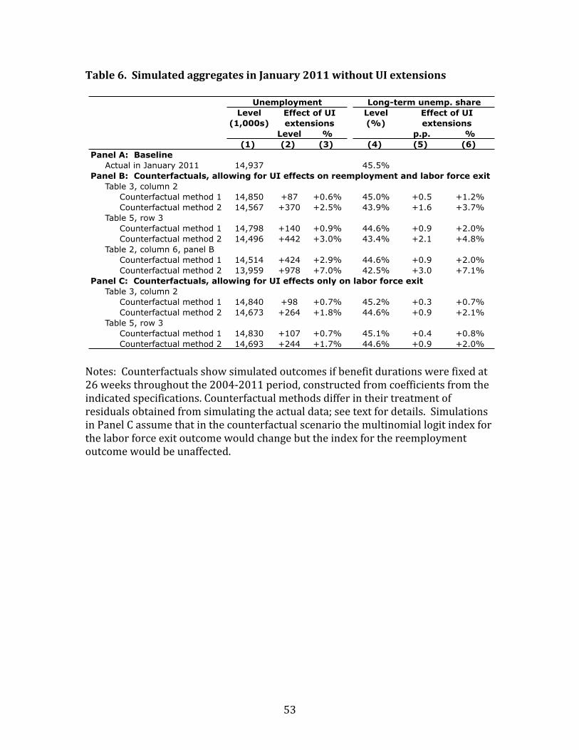
! \Q!

N2=.&'L)''O",$.21&3'2##%&#21&;'"+'R2+$2%0'5S((':"18/$1'*A'&F1&+;"/+;''

!!

$%&'()!!N%2-&'0758&25,(!(+%:!(612,5&'9!%2&8%1'(!67!<'-'76&!9205&6%-(!:'0'!76V'9!5&!

T=!:''M(!&+0%2.+%2&!&+'!T##"/T#AA!3'06%9H!8%-(&028&'9!70%1!8%'77686'-&(!70%1!&+'!

6-9685&'9!(3'867685&6%-(>!N%2-&'0758&25,!1'&+%9(!9677'0!6-!&+'60!&0'5&1'-&!%7!

0'(6925,(!%<&56-'9!70%1!(612,5&6-.!&+'!58&25,!95&5d!(''!&'V&!7%0!9'&56,(>!!G612,5&6%-(!

6-!O5-',!N!5((21'!&+5&!6-!&+'!8%2-&'0758&25,!(8'-506%!&+'!12,&6-%165,!,%.6&!6-9'V!7%0!

&+'!,5<%0!7%08'!'V6&!%2&8%1'!:%2,9!8+5-.'!<2&!&+'!6-9'V!7%0!&+'!0''13,%41'-&!

%2&8%1'!:%2,9!<'!2-577'8&'9>!

!

Level % p.p. %(1) (2) (3) (4) (5) (6)

Panel A: BaselineActual in January 2011 14,937 45.5%

Panel B: Counterfactuals, allowing for UI effects on reemployment and labor force exitTable 3, column 2

Counterfactual method 1 14,850 +87 +0.6% 45.0% +0.5 +1.2%Counterfactual method 2 14,567 +370 +2.5% 43.9% +1.6 +3.7%

Table 5, row 3Counterfactual method 1 14,798 +140 +0.9% 44.6% +0.9 +2.0%Counterfactual method 2 14,496 +442 +3.0% 43.4% +2.1 +4.8%

Table 2, column 6, panel BCounterfactual method 1 14,514 +424 +2.9% 44.6% +0.9 +2.0%Counterfactual method 2 13,959 +978 +7.0% 42.5% +3.0 +7.1%

Panel C: Counterfactuals, allowing for UI effects only on labor force exitTable 3, column 2

Counterfactual method 1 14,840 +98 +0.7% 45.2% +0.3 +0.7%Counterfactual method 2 14,673 +264 +1.8% 44.6% +0.9 +2.1%

Table 5, row 3Counterfactual method 1 14,830 +107 +0.7% 45.1% +0.4 +0.8%Counterfactual method 2 14,693 +244 +1.7% 44.6% +0.9 +2.0%

UnemploymentLevel

(1,000s)Effect of UI extensions

Long-term unemp. shareLevel (%)

Effect of UI extensions

! \"!

N2=.&'M)''O",$.21&3'C/$+1&%92C1$2.'/$1C/,&;'"+'R2+$2%0'5S(('9/%'C/8/%1'&+1&%"+#'$+&,-./0,&+1'"+'5SSTJU('!

!!

$%&'()!!N%,21-(!A!5-9!"!9%!-%&!599!&%!A##cH!5(!5!(15,,!(+50'!%7!(3',,(!<'.6--6-.!6-!

T##b)BA!8%-&6-2'9!&+0%2.+!D5-2504!T#AA>!

p.p. % p.p. %(1) (2) (3) (4) (5) (6)

Table 3, column 2Baseline 67.8% 31.1%Counterfactual method 1 66.4% +1.3 +2.0% 32.9% -1.8 -5.3%

Table 5, row 3Baseline 68.4% 30.4%Counterfactual method 1 67.2% +1.2 +1.7% 32.0% -1.6 -5.1%

Share reemployed Share out of labor forceLevel (%)

Effect of UI extensions

Level (%)

Effect of UI extensions