UNEMPLOYMENT AND PRODUCTIVITY OVER THE

BUSINESS CYCLE: EVIDENCE FROM OECD COUNTRIES

Joaquín García-Cabo Herrero

Master Thesis CEMFI No. 1301

January 2013

CEMFI Casado del Alisal 5; 28014 Madrid

Tel. (34) 914 290 551. Fax (34) 914 291 056 Internet: www.cemfi.es

This paper is a revised version of my Master’s Thesis presented in partial fulfillment of the 2010-2012 Master in Economics and Finance at Centro de Estudios Monetarios y Financieros (CEMFI). I am very grateful to my advisor Claudio Michelacci for his guidance and help throughout these months, and to Samuel Bentolila for his useful comments and careful revision. I also want to thank CEMFI faculty and PhD. students for comments, and finally to my classmates, family and friends, who gave me the strength and support to continue during these 2 years.

Master Thesis CEMFI No. 1301

January 2013

UNEMPLOYMENT AND PRODUCTIVITY OVER THE BUSINESS CYCLE:

EVIDENCE FROM OECD COUNTRIES

Abstract This paper examines the low correlation between cyclical productivity and unemployment: from significantly negative before 1980’s, it has switched sign in several OECD countries and became positive. By using a New Keynesian model with sticky prices, search frictions and variable effort, I find that in the U.S. technology shocks can generate positive correlation between productivity and unemployment, while in Europe non-technology shocks generate the same effect. My results suggest that the increase in size of technology shocks and the reduction of the procyclicality of productivity after a non-technology shock in the U.S. can account for changes in correlation. On the other hand, aggregate demand shocks have gained weight in Europe in the last 20 years and explain the positive sign in the unemployment-productivity correlation in these economies. ! Joaquín García-Cabo Herrero University of Minnesota garci584@umn.edu

1 Introduction

Since the seminal work of Galí (1999), where he pointed out the almost-zero uncondi-tional correlation between productivity and unemployment, there has existed a debateon whether Real Business Cycle models can account for the cyclical fluctuations of thesevariables in the economies, especially the U.S and developed countries.

In particular, there has been certain criticism in the empirical properties of SearchModels. These models (Mortensen & Pissarides, 1994) predict that labor productivityand employment should be positively correlated. There, changes in productivity pro-duce shifts in labor demand, leading to a reduction in the level of unemployment ofthe economy. The effect is summarized as follows: an increase in productivity increasesthe surplus of the worker-firm match. This extra surplus motivates firms to post morevacancies as the demand of labor is increased, and consequently, as vacancies are filled,unemployment in the economy is reduced.

This master thesis tries to provide the literature with estimates of these relationshipsfor a larger sample of OECD countries than the US for which quarterly data on bothunemployment and employment, productivity, total hours and vacancies is collected andreport the results. The analysis will also be replicated for a larger group of countriesdrawn from the Total Economy Database of the Conference Board.

Initially, I describe the sources of the data and time period covered. I have estimatedthe correlation of cyclical fluctuations between productivity, unemployment, employ-ment, vacancies, and vacancies unemployment (v-u) ratio. As a remarkable finding,correlation in the US has switched sign in the mid 1980’s: from being -0.45 between1970 and 1984, in the last 20 years it has increased an exhibits a correlation of 0.07.This result is not isolated for the US, and it is also present in UK, Sweden or Spain. Infact in Spain, it is significantly positive for all the 40 years covered, resulting in a strongcorrelation coefficient after 1984. By performing a graphical analysis of the evolutionof these cyclical components in each of the economies , the sign of the correlation canbe more easily identified.

Changes in correlation might be the result of the counteracting effects of technol-ogy and non-technology shocks in the economy. By performing a bivariate VAR forproductivity and unemployment in the countries chosen, I can account for the effect oftechnology and non-technology shocks on the previous labor market measures. In theU.S., a technology shock, which is assumed to have a permanent effect on productivity,increases unemployment temporarily, generating a positive correlation between thesetwo variables. On the other hand, a non-technology shock, while increasing productiv-

1

ity, decreases unemployment, generating a negative correlation. In Europe, the effectsof both shocks are opposed to the U.S. scenario. A non-technology shock is responsiblefor generating a positive correlation between productivity and unemployment, while atechnology shocks results in a negative correlation.

In order to provide an explanation to these facts, I present a New Keynesian modelas in Barnichon (2010) with three important elements: sticky prices, variable hoursand effort, and search frictions. I have calibrated this model for the U.S. as well as forother OECD countries, and I present the matching of the model and the data for theseeconomies. While the model is able to replicate quite accurately the impulse responsefrom the data in the U.S., it is not very successful in matching the European empiricalevidence. By simulating 40 years of data, I can account for more than 50% of the changein correlation in the U.S. and Sweden, but in Germany or Spain it is again away fromthe data. As a result, I can conclude that technology shocks have increasing importancein the U.S. given that they generate the positive correlation between productivity andunemployment. Therefore, the size of non-technology shocks with respect to technologyshocks in the U.S. might have reduced after 1984.

In Europe, where the model fails to replicate the impulse response of the data, ag-gregate demand shocks are the driving force of the positive correlation observed after1984. In fact, by examining impulse responses after 1984 for the U.S., the cyclical re-sponse of productivity to non-technology shocks has became less negative, approachingthe effect observed in Europe. This also provides an explanation besides the relativeincrease in the size of technology shocks of why correlation between productivity andunemployment has increased.

Although limited, the empirical work that has accounted for the relationship be-tween unemployment and productivity, has also recognized the low correlation foundin the data and highlighted the existing criticisim to business cycle models. Shimer(2005) sustains that the Pissarides model cannot account for the volatility of labormarket variables as observed in US data. Galí and Gambetti (2009) report a declinein the correlation between total hours in productivity starting in the 1980’s. More-over, Barnichon (2010) defends that in the U.S. the low correlation between cyclicalunemployment and productivity hides a large sign switch in the mid-1980’s: from sig-nificantly negative the correlation became significantly positive over the business cycle.His claim is that some structural changes can account for the vanishing procyclicalityof labor productivity starting in the 1980’s: increasing hours per worker elasticity anda more flexible labor market. These changes, together with the fact that volatility ofemployment has increased relative to the volatility of output but has decreased relative

2

to hours, are Barnichon’s argument against RBC theories. However, his analysis isreduced to a single country, the US, and it is not performed in other economies in orderto test its generality. My contribution, therefore, lies in the extension of this analysisto a larger number of countries, such that this relationship can be further investigated.

Regarding the structure of the paper, in section 2 I provide a description of the dataused, descriptive statistics, and I present the correlation between productivity, unem-ployment, employment, vacancies and v-u ratio for OECD as well as Latin Americancountries. In section 3, I present the empirical approach and the model. In section 4 Iprovide a comparison of the responses of the model and the data and the main findings.Finally in section 5 presents my conclusions of the topic.

2 Data description

In order to test whether search models can account for the correlations implied bythe data and to be able to compare cross-countries differences, I will first start bydescribing the different sources of my data set. I will also develop a descriptive analysisof some of the variables of the data set to illustrate the labor market differences acrosscountries, and finally some evidence on correlations between productivity, employmentand unemployment will be presented. This will be the starting point for the rest ofthe paper, as heterogeneity across countries provides a rationale for the study of thebehavior of these variables over the cycle.

2.1 Data sources

This paper is mainly focused on a quarterly analysis of the labor market outcome,although some yearly basis results are presented.

Firstly I will describe the sources chosen for the quarterly analysis. The countriesselected for this purpose are Australia, Canada, France, Germany, Italy, Japan, Norway,Portugal, Spain, Sweden, United Kingdom and United States. Quarterly data on GDP,employment, unemployment, hours worked, vacancies and other variables of interest iscompiled from the OECD. In order for results to be as much comparable and reliableas possible, I tried not to used a different source unless it was necessary. Hence, thefollowing data were not available in the OECD database, and I obtained them from theindicated sources: vacancies from the US and Canada is the Help-Wanted Index (fromJOLTS and Statistics Canada, respectively); unemployment in France comes from theINSÉE (National Institute of Statistics and Economic Studies). Unemployment Ratein Spain is obtained from the INE, and GDP in Sweden is available since Statistics

3

Sweden covers the whole period (in the OECD database started in 1993). The selectionof countries is based also on this issue, as it is difficult to find series that cover longtime spans (1970-2010) even for countries of the OECD. Therefore the time period hasto be reduced in some of them due to unavailability of certain variables.

Following the definition of each variable in the OECD database, unemployment isthe harmonized unemployment level, seasonally adjusted series from the Labor ForceStatistics (MEI). The unemployment rate is defined as the level of unemployed in theeconomy divided by the labor force of the country, this is, the employed and the unem-ployed. The employment level is also from the Labor Force Statistics (MEI) database ofthe OECD, and it is seasonally adjusted. In this paper I use two different definitions ofproductivity. The first one is GDP per employee as a natural measure of productivity.However, as I want my results to be comparable to those in Barnichon (2010) for theUS. I need to construct a series for productivity in terms of output per hour. Hoursworked is not available at the quarterly level, so I imputed a value for output per hourusing productivity per hour annually, as well as production and GDP/Employment,available at a quarterly frequency. In order to check the robustness of this imputation Icompare the resulting series for the US with the quarterly productivity per hour seriesavailable at the BLS and extend the imputation for the rest of countries.

Secondly, I have also constructed an annual database starting in 1950 for a larger setof countries, so I could perform my analysis in developing countries, as well as comparethe results available at a quarterly frequency level with those at an annual level. Data onGDP, hours worked, employment, productivity per hour, and productivity per worker isdrawn from the Total Economy Database (TED) from the Conference Board, and dataon unemployment from the OECD. Due to the unavailability of unemployment dataprior to the 1990’s for Latin American countries, I have performed a partial analysis forArgentina, Brazil, Peru, Chile and Mexico. I have also analyzed the previous OECDcountries with annual data, in order to ensure that my results are not driven by short-term fluctuations.

4

2.2 Descriptive Statistics

The sample periods are 1970I-2010IV for the US, 1971I-2010IV for the UK, 1972III-2010IV for Spain, 1970I-2010IV for Sweden, 1983II-2010IV for Portugal, 1972I-2010IVfor Norway, 1970I-2010IV for Japan, 1970I-2010IV for Italy, 1970I-2010IV for Germany,1970I-2010IV for France, 1970I-2010IV for Canada and 1970I-2010IV for Australia.

Table 1: Time covered by country

As mentioned above, sample coverage is reduced for some countries due to unavail-ability of some series. Vacancies are unavailable for Italy, and in France they start in1989I. In the United Kingdom vacancies end in 2007IV, in Canada in 2003I and inSpain they go from 1977I to 2005I.

For the analysis, data are expressed in logs (except for the unemployment rate) andare detrended using a Hodrick-Prescott filter with smoothing parameter 105 for quar-terly data (as in Shimer, 2005) and for annual data, using a corresponding parameterλ = 6250.

In order to emphasize the diversity of labor markets across OECD countries, Table 2describes the main descriptive statistics for the sample. Panel A reports the mean of theunemployment rate, employment, GDP and hours worked across countries. ContinentalEuropean countries (Germany, France) as well as the UK present higher unemploymentrates compared to the US. But in Europe there are wide differences across Northernand Southern countries. While Norway and Sweden present the lowest unemploymentrates of the sample of countries analyzed, except for Japan; south european countries(Italy, Portugal and Spain), have high unemployment rates for the whole time periodselected.

5

6

It is especially shocking the case of Spain, where the mean of its unemploymentrate (14.19%) almost doubles the rest of the countries. The standard deviation ofeach variable for each country is presented in panel B, and the volatility with respectto the US in panel C. The main conclusions we can draw from these two panels arethat unemployment is more volatile than the other variables, and, in particular, thatthe US exhibits less volatility than Southern Europe in employment and employment,but higher in unemployment. However, the opposite picture emerges when we payattention to GDP, which is definitely more volatile in the US than in Europe, Canadaand Australia.

Finally, panel D exhibits the first order autocorrelation for each of the variables.Unemployment is very persistent in all countries, with a coefficient above 0.85 for al-most every country, except for Norway, Italy and Japan. Employment, GDP and hoursworked are less persistent, and the degree of persistency relative to other countries isusually maintained across variables. In other words, Spain presents a higher autocorre-lation in all these variables, compared to Italy. Nevertheless, major differences are notpresent across countries and all the coefficients are similar.

2.3 Correlations between labor productivity and labor input measures

Table 3 presents a correlation analysis between hourly productivity, employment (e),unemployment (u), vacancies (v) and the labor market tightness ratio v/u for thequarterly data of US, Spain and Germany1. Data are detrended using a Hodrick-Prescott filter with smoothing parameter 105, and the results are not changed by usingdifferent smoothing parameters. Labor productivity measured either as output per houror as output per worker is negatively correlated with unemployment in the 1970-1984period2 in most OECD countries.

These results initially document the degree of heterogeneity present in labor marketsacross countries. Especially in the U.S. the estimate (-0.45) is in line with Shimer (2005)result for a longer period 1948-2003. However, this correlation is very weak compared towhat search models suggest. In a similar fashion, employment exhibits a weak positivecorrelation with productivity, becoming even negative for some countries.

It is even more shocking that after 1984, in line to Barnichon’s finding for the U.S.,these correlations have become even weaker and have switched sign for several countries.Besides the U.S., Sweden, Norway, U.K. or Italy are some examples of this fact, for

1Data are in log base and the analysis for the whole database can be found in Appendix A2The decision to choose 1984 as the end of the first time period is based on comparability of the results to those in

Barnichon (2010) and also on the break implied in McConnel & Pérez-Quiros (2000).

7

both employment and unemployment. An special case to mention is Spain, where thecorrelation between productivity and unemployment (employment) has traditionallybeen positive (negative), and after 1984 it has increase, so that cyclical components ofboth variables co-move positively (negatively). In fact, correlation between productivityand unemployment for 1985-2007 is 0.80, with the opposite sign if employment is used.Vacancies and labor market tightness are also negative, suggesting that the predictionsof search models in this economy will not be validated by the data. These resultsare maintained when performing analysis with output per employee as a measure ofproductivity, and also with annual data for OECD, as well as Latin American countries.

Table 3: Correlations using GDP per hour

Tables can be found in the appendix, but the main claim is that the Southern Eu-ropean, as well as Latin American evidence is hard to reconcile with the predictionsof the traditional search models. Productivity and unemployment tend to move to-gether, with an even higher positive correlation after 1984. In order to go deeper into

8

these results, by comparing the cyclical components of productivity, employment andunemployment, a clearer view arises.

In Figure 1, I present these cyclical fluctuations for Spain. The vertical lines repre-sent CEPR recession dates.3, and it is noticeably how productivity and unemploymentmove together after 1980, and specially the last 5 years of data, the magnitude of thefluctuation is the same. Moreover, these fluctuations for productivity are, for 2000-2010,countercyclical. While in the 2000’s Spain was experiencing a boom in its economy,productivity exhibits a decreasing pattern, and only it starts to increase in 2007, whenthe recession had already started.

These findings are again confirmed by repeating the exercise with annual data. Inparticular, Latin American countries exhibit a similar pattern, that coincides with theone found in Spain. In this same group, Portugal and Italy could be included. Labormarkets of these countries may have common features that lead to this result. How-ever, different liberalization and regulatory processes lead to differences in labor marketinstitutions that cannot solely account for these facts. Some common cultural or un-observed component could be a plausible explanation. However, this exercise requiresfurther research to obtain accurate conclusions.

Figure 1: Cyclical Components of Productivity, Employment and Unemployment in Spain

3These cyclical fluctuations have been plotted for several countries in this exercise and can be found in Appendix B,also with CEPR recession dates for European countries, and NBER recession dates for the US

9

3 Empirical Strategy

After finding that the correlation between productivity and unemployment ( denotedfrom now on as ρ) has switched sign after 1984, it is necessary to understand what forceis driving such a change. Using a bivariate VAR for productivity and unemployment,and imposing the long run restriction that technology shocks have a permanent effecton productivity, I can identify which shock has an outstanding presence in each ofthe economies. Previous findings by Barnichon (2010) suggest that in the U.S. positivetechnology shocks that increase productivity affect unemployment in the same direction,while demand shocks have the counteracting effect. However, the analysis of a greaternumber of countries with heterogeneous labor market outcomes will draw additionalinformation to account for the change in ρ.

3.1 The effects of technology and non-technology shocks on productivityand unemployment

In order to understand how the impact of different technology and non-technologyshocks affect on labor correlations, I proceed as in Galí (1999)4 and I estimate a bivariateVAR with unemployment and productivity:

(∆xt

ut

)= C (L)

(εatεmt

)= C(L)εt

where xt is (logged) labor productivity, ut unemployment, C(L) an invertible matrix

polynomial and εt the vector of structural orthogonal innovations, where εat denotestechnology shocks and εmt denotes non-technology shocks. A long run restriction isimposed on technology shocks to have permanent effects on labor productivity, whilenon-technology shocks have temporary effects. Hence, technology shocks are the onlyshocks to have a long run effect on productivity.

So as to obtain comparable results, I repeat this exercise for both measures of pro-ductivity (per hour and per employee), resulting in similar responses 5. Effects oftechnology and non-technology shocks show how countries differ in their productivity

4I am aware of the criticisms of this approach, especially by Chari , Kehoe, and McGrattan (2008), and mine maysuffer from identical comments. In particular, a VAR with a small number of lags is a poor approximation to the model’sVAR.

5From now on, I am going to focus my explanations in productivity as GDP per hour, as it is the way it is modeledlater, and what other authors have used, i.e. Barnichon or Shimer.

10

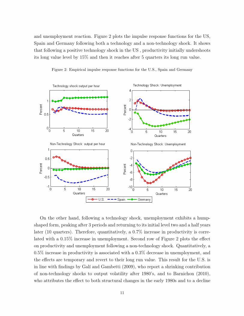
and unemployment reaction. Figure 2 plots the impulse response functions for the US,Spain and Germany following both a technology and a non-technology shock. It showsthat following a positive technology shock in the US , productivity initially undershootsits long value level by 15% and then it reaches after 5 quarters its long run value.

Figure 2: Empirical impulse response functions for the U.S., Spain and Germany

On the other hand, following a technology shock, unemployment exhibits a hump-shaped form, peaking after 3 periods and returning to its initial level two and a half yearslater (10 quarters). Therefore, quantitatively, a 0.7% increase in productivity is corre-lated with a 0.15% increase in unemployment. Second row of Figure 2 plots the effecton productivity and unemployment following a non-technology shock. Quantitatively, a0.5% increase in productivity is associated with a 0.3% decrease in unemployment, andthe effects are temporary and revert to their long run value. This result for the U.S. isin line with findings by Galí and Gambetti (2009), who report a shrinking contributionof non-technology shocks to output volatility after 1980’s, and to Barnichon (2010),who attributes the effect to both structural changes in the early 1980s and to a decline

11

on the procyclicality of productivity. Therefore, technology shocks generate positiveunemployment-productivity correlations.

In Europe these patterns do not necessarily appear. Except for some countries, suchas Sweden, in Spain and Germany, a non-technology shock has an effect on unemploy-ment of the same sign. Following the shock, productivity initially decreases, reachesits trough and returns to its initial level. Similarly, unemployment mimics produc-tivity, and goes initially down. Non technology shocks in Europe result in positiveunemployment-productivity correlations.

These differences seem hard to reconcile with the initial scenario in the U.S.. Mostimportantly, these result suggests that, in order to account for the increasing correlationof productivity and unemployment over the years, technology shocks will have a higherimportance in the U.S., while demand shocks will be the driving force underlying inEurope for changes in correlations.

3.2 A New-Keynesian Model with Unemployment

The interaction between technology and non-technology shocks is driving, up to animportant extent, the changes in correlation between productivity and unemploymentacross countries. This section contains a New Keynesian model with search unemploy-ment as in Barnichon (2010), that will be tested not only for the US, but also for theOECD countries analysed in the previous section. Non-technology shocks are inter-preted as aggregate demand or, more concretely, as monetary shocks6and technologyshocks are orthogonal to monetary shocks . The economy is characterized by threeagents: households, firms and a monetary authority, and relies on three importantpillars: sticky prices, search unemployment, and variable effort and labor hours.

3.2.1 Households

The economy is characterized by the existence of a continuum of households of measureone. Families make decisions on consumption and money holdings in order to maximizetheir expected lifetime utility, as in Merz (1995) and Andolfatto (1996). There are nt

employed workers who receive the wage payment wit from firm i for providing hourshit and effort per hour eit, and 1− nt unemployed workers who receive unemploymentbenefits bt. The individual disutility from working is g(hit, eit).

The representative family maximizes:6This is claimed by Barnichon (2010) to be a parsimonious and tractable way of introducing demand shocks. He

shows that monetary policy shocks display a similar volatility drop to the one experienced by non-technology shocks inthe mid-1980‘s.

12

Eo

∞∑

t=0

βt

[ln (Ct) + λmln

(Mt

Pt

)− nt

ˆ 1

0

g(hit, eit)di

]

subject to

ˆ 1

0

PjtCjtdj +Mt =

ˆ 1

0

ntwitdi+ (1− nt)bt + Πt +Mt−1

with λm is a positive constant, Mt nominal money holdings, Πt total transfers to thefamily, Ct a composite consumption good index, and Pt the aggregate price level.

Barnichon (2010) imposes on the consumption good index the following structure Ct =(´ 1

0 C(ε−1)/εit di

)ε/ε−1

, where Cit is the consumption of good i in period t. Similarly,

the aggregate price level is Pt =(´ 1

0 P 1−εit di

)1/1−ε

. Finally, the functional form of

the disutility of working is as in Bils and Cho (1994) g(hit, eit) =(

λh1+σh

)h1+σhit +

hit

(λe

1+σe

)e1+σeit . λe, λh are positive constants to be calibrated. The (inverse) of worker

per hour elasticity is given by σh, and σe is the elasticity with respect to effort. Aninfinite value for σe generates an inelastic response of effort.

3.2.2 Firms

In this economy, a monopolistically competitive firm which uses labor as an inputproduces each variety of a good. Therefore, there exists a continuum of firms distributedon the unit interval. In period t, each firm i hires nit workers to produce output yit =

AtnitLαit. At is an aggregate technology index, Lit is the labor supply, and 0 < α < 1.

Labor supply is a function of hours and effort with Lit = hiteit.

As each firm is a monopolist in the production of each good, it faces a downwardsloping demand yit =

(PitPt

)−ε

Yt, and they choose prices Pit, to maximize profits takinginto account aggregate price level Pt and aggregate output Yt. We assume that thereare sticky prices (as in Calvo (1983)), so firms cannot adjust prices immediately inresponse to shocks.

The labor market is modeled as in a search and matching framework (Mortensen andPissarides (1994)), where unemployed workers search for jobs and firms post vacanciesat cost ct. The measure of successful matches in a period is given by the usual matchingfunction with a Cobb-Douglas form mt = m0u

ηt v

1−ηt . η represents the elasticity of the

matching function with respect to unemployment, m0 is a positive constant, ut the level

13

of unemployment in the economy and vt the level of vacancies posted by all the firms. Wecan also define θt =

vtut

as the labor market tightness, q (θt) = mt/vt the probability of avacancy being filled in the next period, and λ is the job separation rate in the economy.Finally, the law of motion of employment is given by nit+1 = (1− λ)nit + q(θt)vit.

3.2.3 Monetary authority

This economy is modeled to be non-stationary, with zero inflation in “steady-state” andmoney supply that evolves according to Mt = Atemt. The monetary rule is implied interms of money growth ∆mt = ρm∆mt−1 + εmt + τ cbεat with autocorrelation parameterρm ∈ [0, 1] and εmt is interpreted as an aggregate demand shock, and εat as a technologyshock. As in Gali (1999), if τ cb #= 0, the Central Bank responds in a systematic fashionto technology shocks.

The technology index series is non stationary with a unit root, this is, technologyshocks have a permanent effect on productivity. This is consistent with the long runrestriction imposed in subsection 3.1 on the VAR for persistence of technology shocks.The evolution of technology is denoted by At = Ateat with deterministic componentAt = (1 + ga)At−1, and stochastic component at = at−1 + εat with εat ∼ N(0, σa).

3.2.4 Closing the model

Assuming that firms and individuals are homogeneous, we can average the firms’ em-ployment and define the law of motion for total employment as nt+1 = (1−λ)nt+vtq (θt),with the labor force normalized to 1, so that ut = 1−nt. In this non-stationary economy,vacancy posting costs as well as unemployment benefits grow in line with technology,then ct = cAt and bt = bAt. Finally, in equilibrium Ct = Yt as vacancy posting costsare distributed to the aggregate households (Krause and Lubik, 2007).

3.3 Equilibrium conditions

As the details of the solution of this model can be found in Barnichon (2010), I just willsummarize the first order conditions as well as define the (non-stationary) equilibriumfor this economy.

Household first order conditions

The first order condition for consumption is the usual Euler equation

1

Ct= βEt(1 + it)

Pt

Pt+1

1

Ct+1

14

and for money holdings takes the following form

Mt

Pt=

1

Ct

it1 + it

Firms’ maximization

Firm i will choose a sequence of prices {Pit} and vacancies {vit}, given the aggregateprice level, in order to maximize the expected present discounted value of future profits,subject to the demand constraint, the Calvo price setting condition, the law of motionof employment and the hours/effort choice.

Et

∑

j

βj u′(Ct+j)

u′(Ct)

[Pi,t+j

Pt+jydi,t+j − ni,t+jwi,t+j − ct+jvi,t+j

]

subject to

ydit =(

Pi,t

Pt

)−ε

Yt

yit = yoAtnithϕit

nit+1 = (1− λ)nit + q(θt)vit

wit = γctθt + (1− γ)bt + (1− γ)κ h1+σhitλt

Vacancy posting condition

The optimal vacancy posting condition is

ctq(θt)

= Etβt+1

[χit+1 +

ct+1

q(θt+1)(1− λ)

]

where the shadow value of a marginal worker is given by

χit = −γc

λtθt − (1− γ)

b

λt+ (1− γ)

(1 + σh

ϕ− 1

)κh1+σh

it Yt

Hours per worker is the mechanism driving the incentives of the firms to post morevacancies. When ϕ < 1+σh, the more hours, the larger will be the reduction in the billfor hiring an extra worker7. Following a demand shock, hours grow to satisfy demand,

7With ϕ > 1, the production functions exhibits short run increasing returns to hours. This condition is imposed togenerate procyclical response of productivity to aggregate demand shocks.

15

leading to an increase in the marginal value of a worker. Firms will post more vacanciesand employment will grow.

Calvo price setting condition

A firm i resetting its price at t will satisfy

Et

∞∑

j=0

νjβj

[P ∗it

Pt+j− µsit+j

]Yt+jP

εt+j = 0

where the optimal mark-up is µ = εε−1 and the firm’s marginal cost is sit8.

Non-Stationary Equilibrium

The economy is described by the following system of equations and 5 unknownsθ∗, y∗, h∗, e∗and n∗:

y∗ = y0n∗h∗ϕ (1)

e∗ = e0(h∗)

σh1+σe (2)

βχ∗ =c

q(θ∗)(1− β(1− λ)) (3)

χ∗ = −γcθ∗ − (1− γ)b+ (1− γ)

(1 + σh

ϕ− 1

)κh∗1+σhy∗ (4)

1 = µ1 + σh

ϕ(1− γ)κh∗1+σh−ϕy∗ (5)

n∗ =θ∗q(θ∗)

λ+ θ∗q(θ∗)(6)

where y0,e0 and κ are positive constants9.Variables have been rescaled with technology index At and are denoted by lower-case

letters.8By log-linearizing the Calvo price setting condition, I obtain a standard New-Keynesian Phillips Curve.

9y0 = eα0 , e0 =(

1+σeσe

λhλe

) 11+σe and κ =

λh

1+σh+σe(1+σh)σe

1− γρ (1+σh)

16

4 Confronting the Model with the Data

The impulse response functions from the VAR lead to the evidence that technologyshocks could account for the increase in correlation between productivity and unem-ployment in the U.S., while in European countries demand shocks were those producingpositive comovements of both variables. In order to see to what extent the model I havepresented can account for these different outcomes across OECD countries, I need tocalibrate it with parameters characterizing each labor market. By simulating data withthe model, its empirical performance can be assessed and I can test whether the preva-lence of each of the shocks for each economy can quantitatively account for the changein ρ over time.

4.1 Calibration and impulse responses

I have calibrated the model for 7 countries: the US, the UK, Spain, Sweden, Norway,Germany and Japan, which essentially capture the heterogeneity of the different cor-relations from Section 2. Initially, I have calibrated the US as in Barnichon (2010), toobtain a reliable comparison of the results, taking into account the time period cov-ered here differs from his. After completing this exercise, I have simulated 40 years ofdata for this economy, and compared the response of productivity and unemploymentfollowing technology and demand shocks with the responses in the VAR.

I have proceed in a similar fashion for the rest of the economies, and I have analyzedthe implications of these results for the success of the model and its capacity to matchthe data.

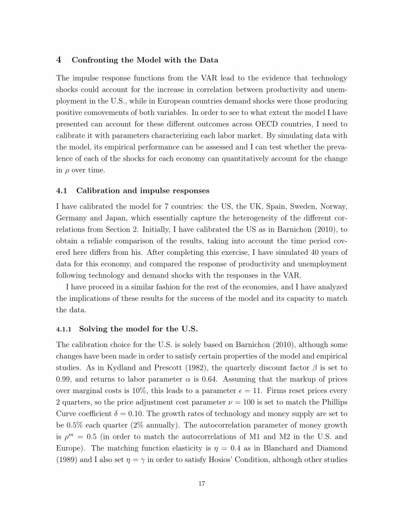
4.1.1 Solving the model for the U.S.

The calibration choice for the U.S. is solely based on Barnichon (2010), although somechanges have been made in order to satisfy certain properties of the model and empiricalstudies. As in Kydland and Prescott (1982), the quarterly discount factor β is set to0.99, and returns to labor parameter α is 0.64. Assuming that the markup of pricesover marginal costs is 10%, this leads to a parameter ε = 11. Firms reset prices every2 quarters, so the price adjustment cost parameter ν = 100 is set to match the PhillipsCurve coefficient δ = 0.10. The growth rates of technology and money supply are set tobe 0.5% each quarter (2% annually). The autocorrelation parameter of money growthis ρm = 0.5 (in order to match the autocorrelations of M1 and M2 in the U.S. andEurope). The matching function elasticity is η = 0.4 as in Blanchard and Diamond(1989) and I also set η = γ in order to satisfy Hosios’ Condition, although other studies

17

suggest this value is very low and should be around 0.7 (Justiniano and Michelacci,2011). A firm fills a vacancy with quarter by probability q(θ) = 0.6, and as in Shimer(2005), the job finding probability is θq(θ) = 0.6. The separation rate is set to λ = 0.10,also as in Shimer (2005), so the jobs last for 2.5 years on average. I have chosen anhours per worker elasticity of 0.31 (σh = 3.2), so as to obtain ϕ > 1, as in Bils and Cho(1994) and in the range of Basu and Kimball (1997).

Finally, Barnichon (2010) sets hiring costs equal to 1% of GDP, and the degree ofaccommodation of monetary policy to technology shocks τ cb = −0.4. The decision to dothis is based on the fact that, as explained in Galí and Rabanal (2004), the policymakerhas difficulties in observing potential output, so technology shocks suffer the risk ofbeing misinterpreted. In such a case, the Central Bank implements a contractionarypolicy, resulting in the negative sign present in this calibration.

Table 4: Benchmark calibration parameters for the U.S.

In Figure 3, I present the impulse response functions following a technology and anon-technology shock for the U.S. and I compare it with the response of a shock thatincreases productivity by 1%, previously obtained from the VAR. Except for deviationsin the response of unemployment following a non-technology shock (it takes longer toreach the trough), the model is quite successful in replicating the responses of the dataconditional on each shock.

In particular, following a technology shock, initially demand does not increase asmuch as productivity because prices are sticky in the short run. Besides, the CentralBank does not accommodate the shock. In order to satisfy demand, firms rely in theintensive margin because they cannot fire workers, and they reduce hours and effort.

18

The value of a marginal worker goes down, and so does the value of posting a vacancy.Firms post less vacancies, and progressively unemployment increases. Productivityundershoots its long run level due to the existence of increasing returns to hours.

On the other hand, the effects of an aggregate demand shock (monetary shock) arethe following. Firms need to increase labor to satisfy demand. However in the short-run, labor is subject to hiring frictions, so firms initially increase effort and hours. Bydoing this, the value of a marginal worker goes up, and firms post more vacancies.This leads to a reduction of unemployment in the economy. As productivity and pricesadjust to the new equilibrium, unemployment also returns to its long run level.

Figure 3: Impulse response functions: Empirical and Model

4.1.2 Empirical response of the model in OECD countries

The interest now relies on testing whether the model can account for the considerablelevel of heterogeneity in labor markets across OECD countries. The model may do wellin matching the evidence in U.S., but its capacity to explain other economies might belimited. For that reason, I calibrate the model again for different countries10, allowing

10Calibration for the US is from Barnichon (2010), the UK, Sweden, Norway and Germany are calibrated followingJustiniano and Michelacci (2011), Spain on Sala and Silva (2005) and Japan on Miyamoto (2009).

19

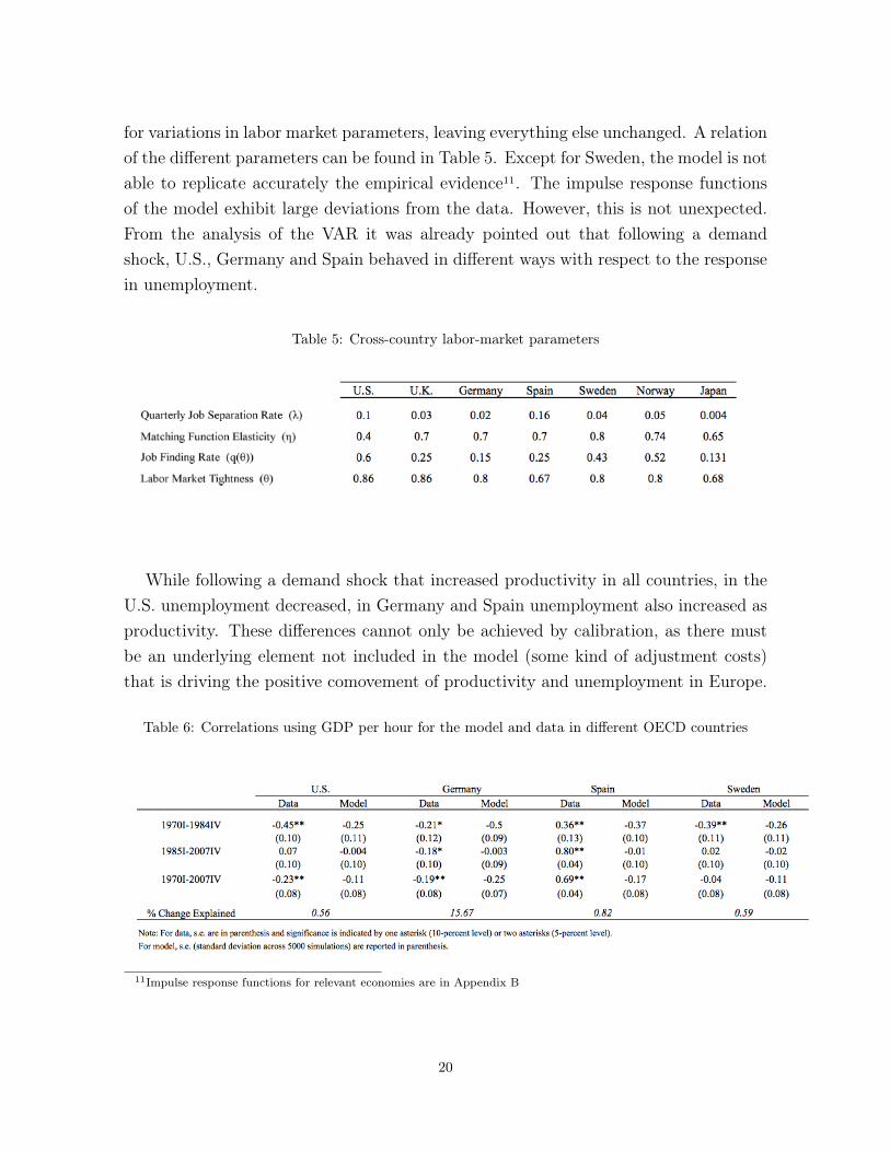
for variations in labor market parameters, leaving everything else unchanged. A relationof the different parameters can be found in Table 5. Except for Sweden, the model is notable to replicate accurately the empirical evidence11. The impulse response functionsof the model exhibit large deviations from the data. However, this is not unexpected.From the analysis of the VAR it was already pointed out that following a demandshock, U.S., Germany and Spain behaved in different ways with respect to the responsein unemployment.

Table 5: Cross-country labor-market parameters

While following a demand shock that increased productivity in all countries, in theU.S. unemployment decreased, in Germany and Spain unemployment also increased asproductivity. These differences cannot only be achieved by calibration, as there mustbe an underlying element not included in the model (some kind of adjustment costs)that is driving the positive comovement of productivity and unemployment in Europe.

Table 6: Correlations using GDP per hour for the model and data in different OECD countries

11Impulse response functions for relevant economies are in Appendix B

20

Nevertheless, there are still other features of the model that can be tested. Theinitial reason for developing such a model was to see if it could replicate the changein correlations experienced by countries after 1980’s, and make an improvement in theprediction of traditional search models. In order to study the sign of the correlationbetween productivity and unemployment, I simulate 40 years of data with the modelcalibrated for each of the economies. For precision, I calculated the correlation betweenproductivity and unemployment over 5000 simulations of the data. I present the resultsof this exercise in Table 6, comparing them with the correlations from Section 2. Thelast row, which presents the change explained by the model is calculated in the followingway: in the U.S., correlation increases 0.52 and 0.21 in data and model respectively.Hence, the variation in the correlation in the model accounts for 56% of the increase incorrelation in data for the same period. Moreover, in the data simulated for Sweden,correlation increases 0.24, almost a 60% of the total change in correlation. On theother hand, for Germany and Spain the model fails to replicate again the empiricalevidence. While in Spain the absolute increase in correlation is high, it does not succeedin achieving the highly positive correlation between productivity and unemployment.And as for Germany, it overestimates the magnitude of the change, which was quitesmall.

Finally I compare the standard deviation of employment 12 and the autocorrelationgenerated by the model with those values obtained from the data. Once again, themodel matches pretty well the volatility of employment and its autocorrelation in theU.S., and also in Germany. Autocorrelation estimates from the model are remarkablyclose to those in data, but the model fails to replicate the volatility of labor outcomemeasures in Europe. As it is shown in Table 7, in Spain and Sweden, the standarddeviation of employment is much lower in the model than in data.

Table 7: Summary statistics of employment for countries and model data 1973-2007

12I have chosen to use employment in t+1 because it is a predetermined variable in the solution of the system ofequations of the model. However, unemployment, which is a state variable, could be obtained using the fact that laborforce is normalized to 1 and results are not affected by these measures. In fact, the correlations are very similar (this ischange is just a vertical translation).

21

All these results confirm that the heterogeneity of labor markets across OECD coun-tries is responsible for the different correlations observed between productivity of un-employment. The relative size of technology shocks versus aggregate demand shocks inthese economies accounts for the changes in correlation observed after 1984. On the onehand, in the U.S. (and possibly Sweden) an increase in the size of technology shocksrelative to demand shocks, is able to produce joint fluctuations of the cyclical com-ponents of productivity and unemployment. In Europe we find the opposite picture:demand shocks have gained relatively more importance after 1984, given that followinga non-technology shock that increases productivity, the effect on unemployment is alsopositive. This could potentially explain the differences in correlations across countries.

Figure 4: Empirical impulse response functions for the U.S., Spain and Germany after 1984

By further examining the differences between the U.S. and Europe, the impulse re-sponse functions of the former after 1984 draw an interesting fact. In Figure 4, followinga positive technology shock, now the effect on unemployment is ambiguous, it initiallydecreases, but after 10 quarters it returns to its initial level and increases again. But

22

more interestingly, the impulse response of productivity and unemployment followinga non-technology shock is more similar to Spain and Germany, compared to the wholesample period. The cyclical response of productivity has diminished significantly, andtherefore, this also leads to an increase in the conditional unemployment-productivitycorrelation.

Some authors13 have examined a reduction in the response of labor productivity, andthe explanation of this finding could go in their direction. However, further researchwould be needed in this area, that is beyond the scope of this thesis. However, a simpleanalysis for the model, in which effort is completely removed from it (calibrating it tobe zero), reveals that the matching of the model for Europe, although still large fromperfect, shows an improvement. In this case, workers could only change hours after theoccurrence of a shock, so productivity does not increase or decrease as much as in thecase with effort. This solution will (partially) conciliate the evidence that in countriessuch as Spain, U.K. or Germany, unemployment and productivity move together inresponse to a non-technology shock, and will better replicate the correlations observedin data.

5 Conclusions

In this master thesis I have exploited the departure of the evidence in correlationsbetween productivity and unemployment from traditional search and matching models.By constructing a data set with quarterly data from the OECD and annual data fromthe Total Economy database, compiled by the Conference Board, I have performedan analysis of the correlations in the cyclical components of productivity, employmentand unemployment in different OECD countries, as well as Latin American countries.The results indicate that the negative correlation predicted by Mortensen and Pissaridesbetween productivity and unemployment is not that strong, and that it has even becomepositive after 1984. Especially, in Southern Europe and Latin countries, this correlationhas been positive before the 1980’s.

In order to evaluate the sources of changes of correlations over time and the het-erogeneity in labor markets over countries, I have first estimated the impulse responsefunctions of a bivariate VAR with productivity and unemployment. The results thatarise from this analysis show that in the U.S., following a positive technology shock thathas a permanent effect on productivity, unemployment rises temporarily and moves in

13Galí and Gambetti (2009) report an smooth and progressive decline in the procyclicality of productivity starting in1970s. Barnichon (2010) attributes these effects to two structural changes: Central Banks became more accommodatingtechnology shocks after 1984, and also to the decline of procyclicality of productivity.

23

the same direction as productivity. However, a non-technology shock with also a posi-tive effect on productivity, although temporary, will decrease unemployment. Thereforean increase in the correlation between productivity and unemployment can be explainedby the increase in the relative size of technology over demand shocks in the US. Nev-ertheless, the picture that emerges in Europe is the opposite. Non-technology shocksproduce shifts in labor productivity in the same direction as unemployment. In theseeconomies, the change in correlation between these two variables lies in the increasedimportance of demand shocks over technology ones.

As an explanation to these facts, I present a New Keynesian model as in Barnichon(2010) with three important elements: sticky prices, variable hours and effort, andsearch frictions. I have calibrated this model for several OECD countries, and I presentthe matching of the model and the data for these economies. While the model isable to replicate quite accurately the impulse response from the data in the US, itsempirical ability to match the evidence in Europe is limited. By simulating 40 yearsof data, I can account for more than 50% of the change in correlation in the US andSweden, but in Germany or Spain it is again away from the evidence. The modelreplicates the prediction of the data, and the most important findings are that whiletechnology shocks have an increasing importance in the US given that they generate thepositive correlation between productivity and unemployment, while in those Europeancountries that experienced a change in correlations, demand shocks play the biggest role.These results impose a constraint in business cycle theories, which claim that cyclicalfluctuations of variables are a recurrent event with many similarities over time andacross countries. In spite of this, these findings suggest that heterogeneity is remarkablyimportant across countries that the evidence from business cycle and search modelscannot be conciliated anymore.

Future lines of research arise when examining the picture in the US after 1984, asit seems that the response of productivity following a non-technology shock has fallensignificantly. Some authors, as Galí and Rabanal (1994) have pointed out this fact,and Barnichon (2010) claims that the reduction in the procyclicality of productivity isdue to a moderation in the volatility of employment with respect to the volatility ofhours per worker, but an increase in the volatility with respect to output since 1984.He also suggests that structural changes have occurred in the labor market in the lasttwo decades, such as a reduction in hiring frictions and more elastic hours per worker.

Moreover, this model is based on sticky prices and variable effort to generate a re-duction in employment following an increase in productivity. Several modifications tothis model may be introduced in order to better conciliate the evidence with Europe.

24

Shimer (2005) proposes including a higher wage rigidity into the model, as in Burdettand Mortensen (1998). As firms have incentives to increase wages, and attract betterworkers away from competitors, the link between productivity and v-u ratio is brokenand this may affect wages and employment in equilibrium. Also introducing flexibleprices would be interesting, and see how unemployment-productivity correlation is af-fected if we rule sticky prices out of the model. López-Salido and Michelacci (2007)also provide an explanation, where the introduction of new technologies leads to anSchumpeterian creative destruction, and obsolete technologies may disappear, leadingto a temporary increase in unemployment.

Finally, the positive correlation between productivity and unemployment over thewhole sample period in Southern Europe and Latin America, but especially in Spain,establishes a future goal for research. The boost of sectors that employed low-skilledworkers, such as construction, followed by the Great Recession in 2007 may have hada role in the correlation in these economies, where productivity fluctuations exhibita countercyclical pattern that mimics the cycles of unemployment. However, a com-mon underlying pattern prevails labor markets in these economies and obtaining anexplanation for this phenomenon is in the future research agenda.

25

References

Andolfatto, David, 1996. "Business Cycles and Labor-Market Search," American Eco-nomic Review , vol. 86(1), 112-32.

Barnichon, R., 2010. "Productivity and unemployment over the business cycle",Journal of Monetary Economics, vol. 57(8), 1013-1025.

Barnichon, R. 2007. “The Shimer Puzzle and the Correct Identification of ProductivityShocks”, CEP Discussion Papers dp0823, Centre for Economic Performance, LSE.

Basu, S., Kimball, M., 1997. “Cyclical Productivity with unobserved input variation”,NBER Working Papers , 5915.

Bils, M., Cho, J., 1994. “Cyclical Factor Utilization”, Journal of Monetary Economics ,33, 319-354.

Burdett, K., Mortensen, D. T., 1998. “Wage Differentials, Employer Size, andUnemployment”, International Economic Review , vol. 39(2), 257-73.

Chari, V.V., Kehoe, Patrick J., McGrattan, Ellen R., 2008. “Are structural VARswith long-run restrictions useful in developing business cycle theory?”, Journal ofMonetary Economics , vol. 55(8), 1337-1352.

Cooley, T., and Prescott, E., (1995), “Economic Growth and Business Cycles”, inFrontiers of Business Cycle Research, ed. by T. Cooley, chapter 1. PrincetonUniversity Press, Princeton.

Gali, J.,1999. “Technology, employment and the Business Cycle: do technology shocksexplain aggregate fluctuations?”, American Economic Review , 89(1), 249-271.

Gali, J., Gambetti,L., 2009. “On the sources of Great Moderation”, AmericanEconomic Journal: Macroeconomics 1(1),26-57.

Justiniano, A., Michelacci,C., 2011. “The Cyclical Behavior of EquilibriumUnemployment and Vacancies in the US and Europe”, NBER Working Papers 17429,National Bureau of Economic Research, Inc.

Krause, Michael U. & Lubik, Thomas A., 2007. "The (ir)relevance of real wagerigidity in the New Keynesian model with search frictions," Journal of MonetaryEconomics, vol. 54(3), 706-727.

Kydland, F. E., Prescott, E. C., 1982. “Time to Build and Aggregate Fluctuations”,Econometrica, vol. 50(6), 1345-70.

López-Salido,D., Michelacci,C.,2007. “Technology Shocks and Job Flows”, Review ofEconomic Studies , 74(4), 1195-1227.

26

McConnell, M. M. , Perez-Quiros, G., 2000. "Output Fluctuations in the UnitedStates: What Has Changed since the Early 1980’s?," American Economic Review , vol.90(5), 1464-1476.

Merz, M., 1995. "Search in the labor market and the real business cycle," Journal ofMonetary Economics, vol. 36(2), 269-300.

Miyamoto, H., 2011. "Cyclical behavior of unemployment and job vacancies inJapan," Japan and the World Economy , vol. 23(3), 214-225.

Mortensen, D., Pissarides, C., 1994. “Job creation and job destruction in the theory ofunemployment”, Review of Economic Studies , 61,397-415.

Sala, H., Silva, J. 2005. “The Relevance of Post-Match LTC: Why Has the SpanishLabor Market Become as Volatile as the US One?”, IZA Discussion Papers 1823 ,Institute for the Study of Labor (IZA).

Shimer, R.,2005. “The cyclical behavior of equilibrium unemployment and vacancies”,American Economic Review , 95(1),25-49.

27

Appendix A: Tables

Table A1: Quarterly correlations using GDP per hour worked

28

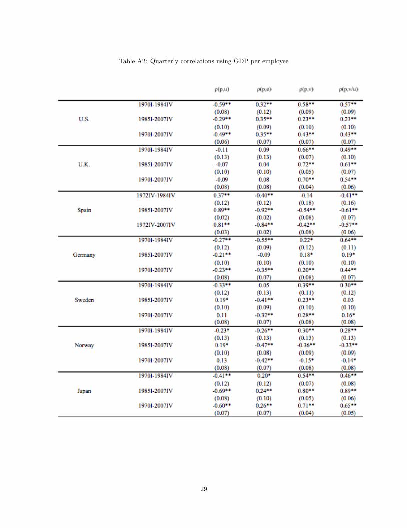
Table A2: Quarterly correlations using GDP per employee

29

Table A3: Quarterly correlations using GDP per employee (Cont.)

30

Table A4: Correlations using GDP per hour worked (Anual)

31

Table A5: Correlations using GDP per hour worked (Anual) (Cont.)

Table A6: Summary Statistics of employment for countries and model data 1973-2007

32

Appendix B: Figures

Figure B1: Cyclical Components of Productivity, Employment and Unemployment in U.S. and U.K.

Figure B2: Cyclical Components of Productivity, Employment and Unemployment in Spain and Italy

33

Figure B3: Cyclical Components of Productivity, Employment and Unemployment in Norway andSweden

Figure B4: Cyclical Components of Productivity, Employment and Unemployment in Germany

34

Figure B5: Cyclical Components of Productivity, Employment in Latin Countries

35

Figure B6: Empirical impulse Response functions for U.K.

Figure B7: Empirical impulse Response functions for Sweden

36

Figure B8: Empirical impulse Response functions for Norway

Figure B9: Empirical impulse Response functions for Japan

37

Figure B10: Impulse Response Functions Sweden: Data and Model

Figure B11: Impulse Response Functions Spain: Data and Model

38

MASTER’S THESIS CEMFI

0801 Paula Inés Papp: “Bank lending in developing countries: The effects of foreign

banks”.

0802 Liliana Bara: “Money demand and adoption of financial technologies: An analysis with household data”.

0803 J. David Fernández Fernández: “Elección de cartera de los hogares españoles: El papel de la vivienda y los costes de participación”.

0804 Máximo Ferrando Ortí: “Expropriation risk and corporate debt pricing: the case of leveraged buyouts”.

0805 Roberto Ramos: “Do IMF Programmes stabilize the Economy?”.

0806 Francisco Javier Montenegro: “Distorsiones de Basilea II en un contexto multifactorial”.

0807 Clara Ruiz Prada: “Do we really want to know? Private incentives and the social value of information”.

0808 Jose Antonio Espin: “The “bird in the hand” is not a fallacy: A model of dividends based on hidden savings”.

0901 Víctor Capdevila Cascante: “On the relationship between risk and expected return in the Spanish stock market”.

0902 Lola Morales: “Mean-variance efficiency tests with conditioning information: A comparison”.

0903 Cristina Soria Ruiz-Ogarrio: “La elasticidad micro y macro de la oferta laboral familiar: Evidencia para España”.

0904 Carla Zambrano Barbery: “Determinants for out-migration of foreign-born in Spain”.

0905 Álvaro de Santos Moreno: “Stock lending, short selling and market returns: The Spanish market”.

0906 Olivia Peraita: “Assessing the impact of macroeconomic cycles on losses of CDO tranches”.

0907 Iván A. Kataryniuk Di Costanzo: “A behavioral explanation for the IPO puzzles”.

1001 Oriol Carreras: “Banks in a dynamic general equilibrium model”.

1002 Santiago Pereda-Fernández: “Quantile regression discontinuity: Estimating the effect of class size on scholastic achievement”.

1003 Ruxandra Ciupagea: “Competition and “blinders”: A duopoly model of information provision”.

1004 Rebeca Anguren: “Credit cycles: Evidence based on a non-linear model for developed countries”.

1005 Alba Diz: “The dynamics of body fat and wages”. 1101 Daniela Scidá: “The dynamics of trust: Adjustment in individual trust levels to

changes in social environment”. 1102 Catalina Campillo: “Female labor force participation and mortgage debt”. 1103 Florina Raluca Silaghi: “Immigration and peer effects: Evidence from primary

education in Spain”. 1104 Jan-Christoph Bietenbeck: “Teaching practices and student achievement:

Evidence from TIMSS”.

1105 Andrés Gago: “Reciprocity: Is it outcomes or intentions? A laboratory

experiment”. 1201 Rocío Madera Holgado: “Dual labor markets and productivity”. 1202 Lucas Gortazar: “Broadcasting rights in football leagues and TV competition”. 1203 Mª. Elena Álvarez Corral: “Gender differences in labor market performance:

Evidence from Spanish notaries”. 1204 José Alonso Olmedo: “A political economy approach to banking regulation”. 1301 Joaquín García-Cabo Herrero: “Unemployment and productivity over the

business cycle: Evidence from OECD countries”.