OTG REPORT No. 1/06

UNDERWATER ACOUSTIC IMAGING: ONE-BIT DIGITISATION1

David G. BLAIR,

Ian S. F. JONES

and

Andrew MADRY

Ocean Technology Group, J05 The University of Sydney

otg@otg.usyd.edu.au

August 2006

ISSN 1442 8075

1 Address correspondence to: D.G. Blair (D.Blair@civil.usyd.edu.au)

Abstract In underwater acoustic imaging (UAI), the combination of a two-dimensional (2-D) array and replicate correlation can produce 3-D images, typically of objects at a range of 2 m. A system already developed achieves the high data acquisition rate needed through one-bit sampling (sensing only the sign of the received signal). Noise added before the one-bit sampling avoids the production of ‘ghosts’ in the image. By simulation and mathematical analysis, the effects of one-bit and added noise are studied for a chirp signal, with a restriction so far to 1-D images (image amplitude versus range). Conditions are given for the avoidance of ghosts and the minimisation of ‘image noise’—noise in the image due to one-bit and added noise. A model of image noise is proposed, which is corroborated by the tests carried out to date. A general formula for the root-mean-square image noise is obtained. It has previously been suggested that filtering the signal after sampling would improve the image. However, it is shown that filtering is unnecessary and indeed makes the image worse. It is shown that a strong target can suppress evidence of a weak target because, when the strength of the return signal is raised, essentially the amplitude of the added noise must be raised to avoid ‘ghosts.’ A general formula, giving the ratio of target strengths such that the weak target has a 50% probability of detection, is obtained.

Contents 1. INTRODUCTION ...................................................................................................... 5 1.1 One-Bit Sampling ................................................................................................ 5 1.2 Pre-Added Noise ................................................................................................. 5 1.3 Dithering and Stochastic Resonance ................................................................. 11 1.4 Oversampling ...................................................................................................... 11 1.4.1 Sigma-Delta Converters ............................................................................. 14 1.5 Imaging Systems ................................................................................................. 15 1.6 The Present Report ............................................................................................ 15 2. THE MODEL ............................................................................................................ 16 2.1 General ................................................................................................................ 16 2.2 Preliminary Discussion of the Later Steps ....................................................... 19 2.3 Dechirping and Beamforming: Details ............................................................. 21

2

2.4 Filtering ............................................................................................................... 24 2.5 Length of Vectors ............................................................................................... 27 3. INITIAL INVESTIGATIONS ................................................................................. 28 3.1 Ghosts .................................................................................................................. 28 3.2 Analytic Signals .................................................................................................. 29 3.3 Autocorrelation Function and a Continuous-Time Approximation .............. 31 3.3.1 Constructive and Destructive Interference ................................................. 34 4. RELINEARISATION; IMAGE NOISE MODEL ................................................. 36 4.1 Relinearisation: Analytical ................................................................................ 36 4.1.1 Linearity in the Mean ................................................................................. 36 4.1.2 LIM: Signal-to-Noise Ratio ....................................................................... 37 4.1.3 An Upper Limit on ............................................................................ 39 4.1.4 Typical Signal Level in a Constant-Strength Interval ........................... 39 4.1.5 Effective Value of ............................................................................. 40 4.1.6 Non-Uniform Distribution of Noise .......................................................... 41 4.1.7 Full Linearity ............................................................................................. 41 4.2 Image Noise Model: Description ...................................................................... 42 4.3 Image Noise Model: Tests ................................................................................. 43 4.3.1 Initial Tests .................................................................................................. 43 4.3.2 Further Tests ................................................................................................ 51 4.3.3 Formula for O Noise .................................................................................... 52 4.3.4 Extent of O Noise ........................................................................................ 53 4.3.5 Conclusion ................................................................................................... 54 5. POWER SPECTRA; FILTERING .......................................................................... 54

maxuu

maxu

5.1 Power Spectra ..................................................................................................... 54 5.2 Filtering ............................................................................................................... 55 5.2.1 An Objection .............................................................................................. 59 6. EFFECT OF NEIGHBOURING TARGETS ......................................................... 62 6.1 Low Sidelobe Level ............................................................................................ 63 6.1.1 Parameters and Estimates ........................................................................... 63 6.1.2 Test for Suppression ................................................................................... 64 6.2 High Sidelobe Level ............................................................................................ 67 6.2.1 Parameters and Estimates ........................................................................... 68 6.2.2 Tests for Suppression .................................................................................. 68 6.2.3 Correcting for Sidelobes ............................................................................. 69

3

6.3 Indirect Suppression ........................................................................................... 71 6.3.1 Counting Independent Values of ( )zp ....................................................... 71 6.3.2 Threshold for Detection .............................................................................. 74 6.3.3 Results of Simulation .................................................................................. 76 6.3.4 Analysis of Results ..................................................................................... 80 6.3.5 Discussion ................................................................................................... 81 6.3.6 Corrections for Sidelobes ............................................................................ 82 6.4 A Comment .......................................................................................................... 84 7. CONCLUSIONS ........................................................................................................ 85 REFERENCES ............................................................................................................... 86 APPENDIX A: SHIFT OF ...................................................................................... 89

jw

APPENDIX B: FILTERING ........................................................................................ 90 B.1 General ................................................................................................................ 90 B.2 Dependence of Power Aliased on E (Qualitative) .......................................... 91 B.3 Varying E and A .............................................................................................. 91 APPENDIX C: GHOSTS IN THE RANGE DOMAIN ............................................. 92 APPENDIX D: TAIL OF ANALYTIC SIGNAL ....................................................... 93 APPENDIX E: MEASURES OF SIMILARITY ........................................................ 95 APPENDIX F: SIDELOBE AND O-NOISE LEVELS .............................................. 96 F.1 Low-Sidelobe Case ............................................................................................. 96 F.2 High-Sidelobe Case ............................................................................................ 97 APPENDIX G: CORRECTION FOR SIDELOBES ................................................. 98 G.1 Sidelobes of Weak Target ................................................................................ 98 G.2 Sidelobes of Strong Target .............................................................................. 100 APPENDIX H: PRINTOUT OF PROGRAM ONEBIT .......................................... 101 H.1 inputsmult.m .................................................................................................... 101 H.2 onebit6.m .......................................................................................................... 105

4

1. Introduction

1.1 One-Bit Sampling One-bit sampling, also called extreme or infinite clipping, is the sampling of a signal in which all that is recorded at each sampling time is whether the signal exceeds some reference value. Commonly the latter is equal to the mean signal value; we consider only this case. Essentially without loss of generality, we suppose that the mean value is zero. For convenience we take the sampler output to be 1+ if the signal is positive and 1− if negative. The one-bit sampler is a bistable system. In the context of radio astronomy, Weinreb (1963) was concerned with measuring the autocorrelation function of Gaussian noise. As he noted, one-bit detection offers a method that is much easier to implement in hardware than many-bit sampling. He calculated the autocorrelation function of the clipped signal, and showed that the true autocorrelation function could be determined from it, with a loss in signal-to-noise ratio (SNR) of 3 to 4 decibels.2 His work drew on earlier work by Van Vleck, described in an internal report in 1943 but not published until 1966 (Van Vleck and Middleton, 1966). Already in this early work, some general features of one-bit sampling can be observed. First, compared to many-bit sampling, a one-bit sampler is both easier to design and cheaper to implement; in fact, at sufficiently high sampling rates, it may be the only practical option. Furthermore by taking a sufficient number of samples and effectively performing an average, often one can recover features of a signal with an accuracy of several bits. 1.2 Pre-Added Noise Let denote the analog input signal value at the ju j th discrete time. The output vv j = of the one-bit converter, as a function of uu j = , is shown by the dashed curve in Figure 1.1. Clearly the response of the converter is highly nonlinear. Such nonlinearity is unfortunate in many contexts, for the following reason. The converter often forms part of a larger system, and often in the larger system it is essential to maintain a linear relationship between the inputs and the outputs. Importantly, a considerable part of any imaging system that uses beamforming requires linearity (since, at least at first sight, the beamforming process works only if the voltage streams at the beamformer are linear superpositions of a common transmitted pulse). Indeed deviations from such linearity in general introduce spurious images or ‘ghosts’ (Steinberg, 1976). Thus, in the context of imaging, one-bit poses a problem.

2 The upper limit is estimated to be ( ) dB92.32log20 10 =π , based on page 37 of Weinreb.

5

A solution to this problem involves adding noise prior to the signal’s entering the one-bit converter. (David Robinson, private communication, drew our attention to the feasibility of restoring linearity by this means.) Let us use the term injector-converter system, or IC system, to mean the combined system of noise-injector-plus-one-bit-converter. Then, subject to conditions, two results can be demonstrated, that amount to the result that the imaging system as a whole is linear after all.

jn

To state the first result, we note that, given the value of uu j = at the j th sampling time, due to the distribution of noise voltages, there is a probability distribution of over the two values, and . This distribution depends on the value of but is independent of the time index

jv1+ 1− u

j . The distribution of determines the expectation

value, jv

jv or v , for the given u . The functional relationship between u and v is

the mean response of the IC system. The first result is that v is proportional to u ; thus the IC system has a response that is linear ‘in the mean.’ The second result is that, for the imaging system considered in this report, during the signal processing, effectively an average of is taken over very many noise samples. As a consequence, the fluctuations in the averaged output are small and the system becomes fully linear.

v

It turns out (Section 4) that three conditions are required for linearity in the mean, while conditions four to six must be added to achieve full linearity. We shall state these conditions in a way that applies more generally than to just the present imaging system. The first condition is the presence of a bistable system. A simple example of the latter is an electric light switch, which may be on or off. Second, the noise voltage should be uniformly distributed over some interval ( )dd ,− . Third, d should be greater than or equal to , the maximum, over time, of the absolute value of the input signal. The fourth condition is that the appropriate statistical parameters of the signal must remain constant over many sampling intervals so that, over time, one can determine estimates of these parameters with low uncertainty. Fifth, the system must actually perform such averaging, or effective averaging. And sixth, the averaging must be performed over a very large number of samples.

maxu

Here we briefly explain why the ‘linear in the mean’ result holds. As will be shown in Section 3, the curve showing the mean response, for uniformly distributed noise, is given by the solid curve in Figure 1.1. The central portion of the curve, occupying the interval

of , is linear. Therefore, if the third condition is satisfied, the relationship is linear over all applicable values of u . ( )dd ,− u

6

Figure 1.1. (i) The response curve of the one-bit converter (dashed). (ii) The mean response curve of the injector-converter system, for noise uniformly distributed in (solid). (iii) The mean response curve for noise voltage following a normal distribution with rms value

( dd ,− )σ (dash-dot). For plotting, the

ratio πσ 2=d has been chosen so that the probability density function of the noise at noise = 0 is the same for the two distributions (note the tangency of the two curves at the origin, in accordance with Equation 4.16). All three graphs assume , not . The normal-distribution curve is accurate rather than schematic.

1±=v dv ±=

We now briefly explain how the ‘mean’ result is extended to full linearity. In the imaging system, the image amplitudes have the form of a weighted average of the . As will be discussed in Section 4, when the number of samples is very large, not only is the mean of each value equal to the weighted average of the

jp kv

jp kv , but the relative size of the fluctuations of about the mean should be small. Full linearity is achieved as the number of samples approaches infinity. When the sixth condition is not satisfied, the system may still be acceptable; in an imaging system, the penalty is that the output contains ‘image noise.’

jp

An alternative way of illustrating the response of the IC system is shown in Figure 1.2. Consider just half a cycle of a sine wave, represented by many discrete values. Figure 1.2(a) shows the half-cycle evaluated at 50 equally-spaced times. We suppose that uniformly distributed noise is injected, with is taken to equal . Figures 1.2(b) to 1.2(d) show, respectively, the added noise , the sum

( )tud maxu

n u′ of the two, and the result of one-bit sampling. As u approaches its maximum value, the output bistable state, represented by , is much more often

v

v 1+ than 1− . In more detail, suppose that the output , as a function of time, is smoothed by taking a moving average over a window of fixed size. Then (Fig. 1.2e) the smoothed output rises, though somewhat erratically, as

rises from to 1. By contrast, in the no-noise case, the rise in output occurs in a single step (at ); in that case the output offers no discrimination between the

v

u 1−0=u

7

different positive values of u . When the total number of samples is changed from 50 to 2000, the output is found to track u much more closely (Fig. 1.2f). We shall see that effectively such a large number of samples is obtained in the underwater acoustic imaging system by using a very long chirp followed by cross-correlation as a kind of averaging.

Figure 1.2 (a and b). Added noise in conjunction with one-bit. (a) The input signal and its value at 50 sampling times. (b) The noise stream.

8

Figure 1.2 (c and d). (c) The total voltage immediately prior to one-bit sampling. (d) The signal after one-bit sampling.

9

Figure 1.2 (e and f). (e) The signal (d), after applying a moving average of size 5 samples. (f) The result of steps (a) to (e), but when the total number of samples is 2000.

10

1.3 Dithering and Stochastic Resonance Historically, the basic results for the IC system flowed from studies of two other systems, which we now discuss briefly for completeness. This subsection is not required for an understanding of the remainder of the report. Dithering arises in the context of an -bit sampler with . Let be the quantisation interval, that is, the interval between adjacent output levels of the sampler (assumed to be the same as the interval between one threshold input level and the next). It was found that the performance of the sampler over a long sequence of samples can be improved by the dithering effect: a carefully controlled amount of noise (dither) added to the analog signal before digitisation reduces, in the mean, the error in the output voltage to a value much less than

n 1>n Q

2Q . For recent work in this area, see Bulsara and Gammaitoni (1996) (a review), Gammaitoni (1995) (which discusses uniformly distributed noise), Gammaitoni et al. (1998) and Gingl et al. (2000). The history of dithering can be traced back to 1948 (Bennet, 1948). Stochastic resonance requires a bistable system and typically involves also a periodic signal that would, if stronger, push the system back and forth between the two states. Typically an increase in the root-mean-square (rms) noise above some ambient level, produces an amplification of the output signal, in the following sense. The input signal

combines with influences having a random component, to produce an output signal . (In general the system also has ‘memory’ of earlier values of

( )tu

( )tu( )tv ( )tv .) Let have

period ( )tu

T . Let ( )tv be , averaged over the times v ...,2,, TtTtt ±± Normally v also has period . It has been found that, under certain conditions, the amplitude of the oscillations of

Tv with time is increased by increasing the noise. This mechanism is called

stochastic resonance. It turns out that often not only the output signal, but also the SNR at the output, can be increased by increasing the input noise. In the latter case the mechanism can make possible the detection of weak signals that are otherwise undetectable. This constellation of results is counterintuitive. Stochastic resonance has been discussed in a vast number of papers, reviewed by each of Gammaitoni et al. (1998), Bulsara and Gammaitoni (1996) and Moss and Wiesenfeld (1995). The concept has been applied in many fields. It was first proposed in 1981 to explain the statistics of the onset of ice ages (Benzi et al., 1981). (There the driving ‘force’ is surprisingly small compared with the change in temperature produced.) Macnamara et al. (1988) applied the concept to laboratory systems: such applications include lasers and tunnel diodes.

( )tu

1.4 Oversampling We discuss oversampling for two reasons. First, in a number of systems in which there is one-bit digitisation, oversampling combined with filtering enables a many-bit output to be recovered. Second, in the present report, Section 5 examines whether this

11

combination produces a similar benefit in the present imaging system. The answer is that the oversampling produces a benefit (simply because it produces more samples for averaging), but that the filtering does not.3 Armed with this knowledge, the reader may wish to skip Section 1.4. It is well known that, given a signal whose positive frequency components are confined to an interval from 0 to B ( B is the bandwidth in Hz), if the signal is sampled at a sampling rate , the signal can be exactly reconstructed from the samples provided that sf

Bf s 2> The critical frequency is called the Nyquist sampling rate.Bf 2N = 4 (The result as stated applies to both a real signal and to an analytic signal. The signal is of infinite length.5) A signal is said to be oversampled when is significantly higher than the Nyquist frequency, particularly when . The ratio

sf

Nff s >>r

s ff 2OSRN == (1.1) is called the oversampling ratio. Oversampling can be used to increase the effective number of bits sampled (e.g. Aziz et al., 1996; Freeman et al., 1999). For simplicity, consider a low-pass signal (it is believed that somewhat similar results apply to band-pass signals). The method used (Figure 1.3) is to take the data stream that results from oversampling, say at one bit, and send it first through a digital low-pass filter, of bandwidth slightly above B . This process is usually followed by downsampling, that is, saving, say, only every sixteenth sample value. (The combination of the filtering and the downsampling is called ‘decimation.’) Consider an analog-to-digital converter defined as follows: a voltage interval ( )WW ,− is subdivided into equal subintervals; given any input voltage, the converter outputs the centre of the subinterval in which that voltage lies. The quantisation interval is

L2

LW 22=Δ (1.2) At each sampling, a quantisation error e is incurred. The ‘power’ of the noise is taken to be 22 ee =σ (in ), where the average is over the probability distribution of . Provided the distribution is uniform, this power comes out to be

2volt e

1222 Δ=eσ (1.3) (The theory of quantisation noise actually makes further assumptions, see Aziz et al., 1996.) Thus, on a decibel scale, we have

( ) (dB) 77.402.6log20log10noise 2e −−== LWσ (1.4)

3 This is the answer in the case of traditional converters; sigma-delta converters were not studied. 4 A similar result applies to band-pass signals of bandwidth B , with the proviso that in general the sampling required involves pairs of samples. The samples in the pair are separated by a fixed time , not necessarily equal to a sf1 . After every sf2 seconds, another pair of samples is taken. 5 The sign may be replaced by provided the Fourier power density at the band edge is not infinite.

> ≥

12

This is the noise when no filtering is applied; if the sampling is at the Nyquist rate, no reduction of this noise is possible by filtering.

L-bitQuantiser

Low-PassFilter

DownSampler

analog

digital

resolution> L bits

Figure 1.3. Decimation, used to increase the effective number of bits sampled.

0-B B-f /2s f /2s

Power density

0

frequency f Figure 1.4. Quantisation noise power density for Nyquist rate sampling (solid curve), and oversampling (dashed). The dash-dot curve shows schematically the power density for a sigma-delta converter and illustrates noise shaping.

Now compare two situations: in the first, sampling is at the Nyquist rate, while in the second, oversampling is used. In the two cases, the quantisation error, and hence the total quantisation noise (per sample), is the same. But (as discussed by Aziz et al., 1996 and Freeman et al., 1999) the error e , as a function of sample number (time), has a distribution of Fourier power density versus frequency that is uniform over the frequency interval ( 2,2 ss ff− ) (Figure 1.4). In the two cases the total powers (area under curve) are the same, but in the second case the power is spread over a wider frequency range, so that much of this noise power lies outside the band ( )BB,− of the signal. (In the first case, none of the noise is outside.) Now the out-of-band noise can be filtered out without detriment to the signal. From Figure 1.4 the noise power is thereby reduced by a factor equal to the oversampling ratio (1.1). Thus the output of the combined process of oversampling and decimation contains a noise signal (the difference of the output from what it would have been with exact sampling), the power of which, , is less than . Indeed from Figure 1.4 and (1.1), we have

n2nσ 2

eσ

13

OSR

22 en

σσ = ; (1.5)

or, using (1.1) and (1.4), ( ) (dB) 01.377.402.6log20log10noise 2 rLWn −−−== σ (1.6)

Thus the quantisation noise is reduced by 3 dB for each doubling of the sampling frequency. Another way of expressing this is that the reduction in noise is equivalent to an increase in the number of bits in the original converter. Comparing the coefficients of r and L in Equation (1.6), we see that each doubling of produces an effective gain of half a bit.

sf

In an underwater acoustic imaging system, the oversampling ratio can be appreciable. For example, in a known practical case that uses an IC system, the OSR is about 2.5 (based on the strict Nyquist theorem and thus based on the maximum frequency component). It therefore appears that (as was suggested by Ian G. Jones and David Robinson, private communication) filtering of the IC output should reduce the noise in the final image, in which case the filtering would be worthwhile. Indeed, as the original signal lies in a pass-band, one would expect a considerably greater improvement by applying a band-pass filter. We conceive of these filters as being applied in addition to the cross-correlation (to be discussed in Section 2), which is itself a kind of filter. In Section 5 a simulation of such filters will be described. Surprisingly, it turns out that such filtering is not beneficial. We shall call converters of the types discussed so far ‘traditional’ converters, to distinguish them from sigma-delta converters. 1.4.1 Sigma-Delta Converters The one-bit converter with pre-added noise is one solution to the problem of handling high sampling rates at relatively low cost. The term sigma-delta converter (e.g. Aziz et al., 1996; Freeman et al., 1999) refers to a class of devices that also solves this problem. Attention is drawn to this converter only because, in the context of imaging, of the known cases where one-bit sampling has been applied, nearly all use the sigma-delta converter. The discussion will be very brief. The devices are also called delta-sigma converters; often the names are written as or ΣΔ ΔΣ converters. Sigma-delta converters do not add noise; they are deterministic. Instead, the converter consists of a digitiser, most often a one-bit digitiser, together with further low-cost circuitry (not described here), such that a quantised output is produced. It turns out that (provided that the sampling interval is short compared to the inverse of the typical frequencies in the signal) the output after averaging, though not quite proportional to the input, is close to being so. The main departure from linearity occurs because there are a few extremely narrow frequency bands within which the Fourier components are strongly enhanced by the converter. This results in ‘auto-oscillations’ or ‘limit-cycle oscillations’—a problem that is well known in the context of digital IIR (infinite impulse response) filters (Bellanger, 1984). Bellanger describes the phenomenon by saying that,

14

even if there is no signal at the input, an oscillatory signal appears at the output. Designers of a sigma-delta converter need to be aware of this problem. Sigma-delta converters have a strong advantage over traditional converters, called noise shaping. Consider for simplicity the case where the signal is limited to a low-pass band. The quantisation noise in the output of the sigma-delta converter is no longer distributed uniformly over an interval of frequency. Instead (Figure 1.4), the power is redistributed within the interval ( )2,2 ss ff− . Power is moved out of the band of the signal, into the remaining part of the interval. Thus the subsequent application of a filter (as for a traditional converter) is particularly effective in attenuating the quantisation noise. Indeed, for a so-called second-order, third-order and fourth-order sigma-delta converter, the reduction in the quantisation noise for each doubling of is no longer 3 dB, but 9 dB, 15 dB and 21 dB respectively.

sf

1.5 Imaging Systems A few cases have been reported in the literature in which one-bit sampling was used in an imaging system. These cases have mainly been applications in the area of medical ultrasound imaging. In all the known cases of medical imaging, the sigma-delta converter has been chosen (for example, Han et al., 2002; Freeman et al., 1997; Freeman et al., 1999; and Kozak and Karaman, 2001). Two other applications of one-bit sampling to imaging have been reported. One is an application to the radio camera (Steinberg, 1984). It appears that one-bit was used at the front end of the sensor devices, without added noise or other embellishment. The article reports that the image quality is hardly degraded, but does not attempt to explain why the nonlinearity causes no problem. Finally, one-bit sampling has been used in underwater acoustic imaging (UAI), in a project carried out in Australia by the Defence Science and Technology Organisation (DSTO) and their collaborators, Thales Underwater Systems and CSIRO (Commonwealth Scientific and Industrial Research Organisation) (see Maguer et al., 2000; Vesetas and Manzie, 2001; Manzie, 2000; and Jones, 1996). The specific aim was to image suspected sea-mines in turbid (muddy) water. The images were judged to be of satisfactory quality. 1.6 The Present Report The present report considers the imaging of a scene by an active sonar with a point or spherical transmitter, largely following the model of Blair and Anstee (2000). The system of ultimate interest contains a two-dimensional (2-D) array of receiving elements for angular resolution of targets and uses a coded pulse or chirp to produce range resolution. The image is thus three-dimensional. In the present report, the scene considered is one-dimensional, that dimension being the range. However, a number of

15

results are obtained, most of which are relevant also to the 3-D imaging system. The study is carried out using both analytic calculations and simulations. Section 2 describes the details of the system considered, including features of a simulation program used in the study. Section 3 discusses ‘preliminary’ investigations: investigations into ghosts, analytic signals and the continuous-time approximation. Section 4 explains in detail why the system is relinearised under the conditions stated in Section 1.2. For a chirp of finite length, the image contains ‘noise’ in addition to the ‘mean’ component of the image amplitude; this image noise is due to the one-bit sampling together with the injected noise. Recognising this fact, the section proceeds to describe a model of the image noise and presents evidence supporting the model. Section 5 investigates the effect of adding a filter and shows that this is not beneficial. Section 6 examines the extent to which, when one-bit sampling is used, the presence of a strong target suppresses the detection of a weak target; the latter may be close to, or far from, the strong target. Conclusions are presented in Section 7.

2. The Model 2.1 General The transmitted signal is a rectangular-envelope, linear chirp of the form

( )

2 0

2 2cos 1

221

Tt

Ttcbttfts c

≥=

<⎥⎦

⎤⎢⎣

⎡+⎟

⎠⎞

⎜⎝⎛ += π

(2.1)

(The chirp is taken to have unit amplitude for simplicity.) Here T is the duration of the chirp, is the central frequency (in Hz) and , the rate of change of frequency with time, is related to the bandwidth

cf bB (Hz) by

TBb = (2.2) The instantaneous frequency is

btf

bttfdtdf

c

ci

+=

⎟⎠⎞

⎜⎝⎛ += 2

21

(2.3)

To avoid unnecessary degradation in the image, only combinations of the parameters are considered such that the chirp is continuous at its ends, that is, the value of the cosine in (2.1) is zero there. Thus the chirp has a whole number of half-cycles. A program, ONEBIT, has been written in MATLAB so that the predictions of the model can be studied numerically. A printout of ONEBIT is included in this report as the final appendix (Appendix H). The program slightly modifies the duration T away from

16

the value that is input so that the chirp contains exactly an even number of cycles.6 The program calculates the value of so that the signal 1c ( )ts is continuous. In this report we consider only the one-dimensional (1-D) case. There is a single receiver, taken to be co-located with the transmitter at the origin. The point targets lie on the positive axis. The received signal at time is z t

( ) ( )∑ −=≡i

iij cztsatuu 2 (2.4)

where and are the strength and location of the i th target and is the speed of sound. (The notation refers to the

ia iz c

ju j th sampling time below.) may have either sign, representing the difference in scattering from a hard or a soft object. It is assumed that there is no attenuation.

ia

The sampling and signal processing proceed as follows (Fig. 2.1). Given the sampling frequency , all sampling is taken to occur at times sf

sj fjt ⎟⎠⎞

⎜⎝⎛ +=′

21 (2.5)

where j is an integer. The transmitted chirp is represented by the stream , given by evaluating (2.1) at the times . As in a real system, the received signal is to be sampled only at a sequence of times that begins after all the chirp has been transmitted but before the first return signal arrives at the receiver.

js

jtt = ju

To proceed, we must take more care over the index j . We choose to label the first element in each computed vector with the index 1=j ; this makes for easy translation into MATLAB.7 For reasons given below, all ‘signal’ vectors such as s and u are chosen to have a common length (equal to a power of 2); the vectors are padded with zeros where necessary. ( s is the vector consisting of the ; and similarly for other vectors.) The centre of the vector s is chosen to correspond to time , so that for the vector s , time is related to the index by

Njs

0=t

( ) sj fNjt ⎟⎠⎞

⎜⎝⎛ −−=

21

21s (2.6)

For , however, there is a time-delay compared to , as the signal must travel to the targets and return. We suppose that the targets are confined to lie between a minimum value of the range and a maximum value . Consider that interval of in which the value of is potentially nonzero. The delay between

u s

minz maxz t( )tu 0=t (the centre of the

chirp) and the centre of that interval is ( ) czzcztf s minmaxmid2 +==≡′δ

6 An even number of cycles is chosen, rather than a whole number of half-cycles, because the mathematics is then simpler. 7 The alternative is to maintain a universal relationship, such as (2.5), between time and the index.

17

Here δ ′ is defined by the equation. Let δ be δ ′ but rounded to the nearest integer. In the program, the time-index relationship for u is adjusted by a shift in the index by δ so that, as nearly as practicable, the centre of the return signal lies in the middle of the vector of length —as it does for . Therefore the relationship for is N s u

( ) sj fNjt ⎟⎠⎞

⎜⎝⎛ +−−= δ

21

21u (2.7)

The relationship (2.7) also applies to the streams u′ , and q to be introduced shortly. v

transmitter scattering sensorelement add noise one-bit

sampler

calculateanalytic filter cross-

correlatorbeam-

forming

sphericalwave

scatteredwave

u u ′ v

va qa w a image

s

sah

analog digitaln

Figure 2.1. The signal processing as modelled and the physical processes assumed to precede it. Optionally and independently, the ‘add noise’ and the ‘filter’ boxes may be bypassed and the one-bit sampler may be replaced by an exact sampler. As discussed in Section 1.2, it is expected that one-bit sampling leads to good images under a wide range of conditions, provided that before sampling, random noise of suitable amplitude added to the received signal. Thus in the program, optionally, random noise is now added to the received signal to produce the signal-with-noise jn

jjj nuu +=′ (2.8) (If no noise is added, .) The noise voltages at different values of jj uu =′ jn j are taken to be statistically independent. Each such noise voltage is taken to be uniformly distributed over an interval , where , which is independent of

jn( dd ,− ) d j , is the noise

amplitude. Thus we have (for each j )

( )dn

dndd

n

j

jj

≥=

<<−=

0

21Pr

(2.9)

Here and elsewhere, Pr denotes the probability density function of its argument, or the probability itself if the distribution is discrete. Actually it is known in advance that the signal is identically zero outside the time interval

ju

18

( ) ( ) 2222 maxmin TzctTzc +≤≤− (2.10) To avoid introducing noise that serves no purpose and tends to degrade the image, in ONEBIT noise is added only at times satisfying (2.10). The number of such times, L , is

( )( )[ ] 12 minmax ±+−= sfTzzcL Likewise, the output of the step immediately below is put equal to zero outside the interval (2.10).

jv

The next operation produces the digitised signal , either by exact sampling (jv jj uv ′= ) or by one-bit sampling. In the latter case we have

0

0

<′−=

>′+=

j

jj

ud

udv (2.11)

In a practical system, normally unity is used in place of d on the right-hand side. Later (Section 4.1.1) it will be seen why, in the theoretical development, it is advantageous to use . In any case, only the sign of d ju ′ is preserved. (The sign could be represented using 1 or 0, but here it is convenient to use +1 or –1, or d+ or d− . Exact sampling is of course an impossible ideal, but a good approximation to it is available by sampling to a sufficient number of bits.) At this point it is well to define two options for the overall system that are of special interest, to be called E sampling and O sampling. In E sampling (E for exact), the sampling is exact and there is no added noise. In O sampling (O for one-bit), one-bit sampling is performed and there is added noise; furthermore the noise amplitude satisfies the condition (third condition in Section 1.2, repeated below as Equation 4.3). For both types of sampling, it is implied that no filtering is performed unless stated otherwise.

maxud ≥

We note that the sampling frequency must satisfy the Nyquist relation (Section 1.4), that is, must be at least twice the effective maximum frequency occurring as a component in the chirp signal. This condition may be written as

sf

( )[ ]22 Bff cs θ+≥ where it is expected that we may take 1.1=θ if the chirp is very long. (At this juncture, we do not attempt to invoke a Nyquist-type relation based on the fact that the signal is a band-pass signal with bandwidth B .) 2.2 Preliminary Discussion of the Later Steps In this preliminary discussion, some technical complications in the mathematics are postponed to Sections 2.3 to 2.5, in order to concentrate on the key concepts. In accordance with the program discussed in Section 1.4, optionally, filtering is now applied to the signal to remove most of the out-of-band components of that signal. In the frequency domain, this operation consists of multiplication by a filter function

v( )fH

19

( = frequency). The resulting signal is denoted in time domain by . For the present we represent the relationship in time domain symbolically in terms of vectors by

f jq

( )vq filter= (2.12) where filter is a linear function. Details are given in Section 2.4. In order to obtain good range resolution in the positions of the targets, the recorded signal is then cross-correlated with a replica of the transmitted signal, to produce the dechirped or correlated signal (Rihaczek, 1985; Ziomek, 1985; Burdic, 1991; Kino, 1987):

jw

∑ −+=k

jkkj qsM

w 12 (2.13)

Here ; to within , TfM s= 1± M is the number of sample points in the ‘proper chirp.’ In (2.13), in practice is confined to the k 1±M values for which is nonzero. In general the range of k is further restricted because may be zero. (The normalizing constant

ks

1−+ jkqM2 in Eqn 2.13 has been chosen so that, when there is exact sampling with no

added noise, and there is a single target with strength unity, the peak value of the correlated signal (that is, maximised over jw jw j ) is unity for a chirp with many cycles.8) (The ‘ ’ in the subscript reflects the fact that the first element in each vector is labelled with , not

1−1=j 0=j .) This cross-correlation process is also called

dechirping. In the present context the replica of the transmitted signal is also called the reference signal. Note that the reference signal is not quantised to one bit.9 We define the cross-correlation operation ⊗ by

( ) 1−+∑=⊗ jkk

kj hghg (2.14)

(Some authors replace by its complex conjugate on the right-hand side.) Then (2.13) may be written

kg ∗kg

( jj )M

w qs⊗=2 (2.15)

The time-index relationship for w (expression for ( )wjt ) is different from that for and is derived in Section 2.3.

u

Finally, beamforming is carried out to produce an image. When there are many elements, beamforming is done by a delay-and-add procedure applied to the signals at the various receiver elements. In the 1-D case there is only one element; hence there is no adding. But there is ‘delay,’ in the sense that the time of flight determines the

8 When we move from one to three dimensions, the result is no longer unity, because of spherical spreading. 9 There appears to be little point in investigating the effect of digitising the reference signal to one bit. The reason is that, as the cross-correlation is performed in software, there is no difficulty performing it with the exact reference signal.

20

corresponding position being imaged. Thus we obtain the image amplitudez ( )zp car at

the discrete set of positions ( )wjct21 :

( ) jj wctzp =⎥⎦⎤

⎢⎣⎡ = w

21car ; (2.16)

thus is forced to be positive. The superscript refers to the modulated image (containing a carrier wave), as explained in the next subsection.

carp

2.3 Dechirping and Beamforming: Details We now discuss the later steps in the signal processing; as an exception, filtering is postponed to Section 2.4. In respect of the dechirping and beamforming, Equations (2.13) and (2.16) do not tell the full story. The image formed according to these equations is modulated as a function of : contains a rapidly oscillating factor—a ‘carrier wave’—that does not correspond to any oscillation in the scene being imaged. The carrier wave can be eliminated by the use of what is called the analytic signal (e.g. Bellanger, 1984, p. 244). A brief and by no means complete discussion of the latter will now be given.

z ( )zpcar

From any physical signal —called the in-phase component—one can calculate what is called the quadrature component (the latter is a fictitious signal). When the latter signal, multiplied by

( )tx

1−=i , is added to the in-phase component, the result is the analytic signal, denoted by . The analytic signal has the property that its Fourier components at all negative frequencies are zero. Indeed this fact provides the simplest method of computing the analytic signal. (The method is: Given the Fourier transform of the in-phase component, double each of its positive-frequency components and replace its negative-frequency components by zero. Then take the inverse Fourier transform.) An important relationship is that the quadrature component is obtained from the in-phase component by taking each Fourier component of the latter and shifting its phase by

( )tx a

2π . The above results are stated for signals as a function of continuous time, but require only slight modification for the case where the signal is sampled at discrete times—or rather, the case in which time is discrete but is also ‘wrapped around.’ The latter means that the time at the last or th element of any signal vector is considered to be followed by the time at the first element; in effect, the elements are arranged around a circle. This combination of discreteness and wrapping occurs in the context of the discrete Fourier transform, and in particular, the context of the fast Fourier transform (FFT).

N

For future use, we introduce some mathematics. We follow the definition of the FFT used in MATLAB:

21

( ) ( )

( ) ( ) ( )∑

∑

=

−−−

−−

=

==

==

N

m

mjNmj

mjN

N

jjm

XN

xXx

xXxX

1

11

11

1

1 means ifft

means )(fft

ω

ω (2.17)

where is the length of the vectors and N ( )NiN πω 2exp −= . (Strictly speaking, what Eqn 2.17 defines is the discrete Fourier transform; the ‘fast Fourier transform’ refers to a fast method of calculating the discrete Fourier transform.) In (2.17), the frequency associated with , and hence with , is m mX

( ) Nfmf sm 1−= (2.18) The zero-frequency component appears at 1=m . Because there is wrap-around in the frequency domain as well, the last 2N elements are best thought of as giving the negative-frequency components. Then the maximum frequency occurs at 12 += Nm (as also does the negative frequency with the largest absolute value). The power density or spectral density (or Fourier power density) of the signal x at the ‘frequency’ m is defined to be 2

mX , while the power (or total power) of x is 22 ∑∑ =

j jm m xNX (2.19)

where the equality to the last expression is well known. In the context of the FFT, the convolution theorem, applied to the cross-correlation operation, is

( ) mmHG∗∗ =⊗hgfft (2.20) where ∗ denotes complex conjugate and it is understood that the th element of the left-hand side is to be taken. In (2.20), the operation

m⊗ is defined by (2.14) but with wrap-

around now enforced; that is, when an index such as 1−+ jk goes outside the interval , the index is interpreted modulo . N ..., ,1 N

We now apply the above concepts to images. The real (in-phase) transmitted signal

determines the transmitted analytic signal ( )ts ( )ts a . Similarly the vector s , or , when processed according to the above rules but with the FFT replacing the Fourier transform, determines a corresponding analytic signal . The latter is an adequate representation of

, subject to a check that there is no aliasing due to the finite length of the vector. (This check is carried out in Sections 2.4 and 2.5.) The streams , , , and

are defined similarly in terms of , etc., and the same comments apply as for . Subject to the insertion into (2.12) of the filter function from Section 2.4, all these quantities are now defined. It can be shown using (2.13) that

js

ajs

( )ts a

aju a

ju′ ajv a

jq ajw

ju ajs

a1

a1

aa 12−+−+ ∑∑ ∗∗ == jk

kk

kjkkj qs

Mqs

Mw (2.21)

22

(Note the absence of the superscript a from the q factor in the middle expression.) For computation it is convenient to use the frequency-domain version of (2.21); from (2.20) and (2.14) this is

( ) aaa 1 mmm QSMW ∗= (2.22) Here, for example, is the th component of the FFT of . The final, or unmodulated, image is formed by using the absolute value of the analytic in place of

itself (in-phase) on the right-hand side of (2.16); thus the image amplitude is

amS m a

jsw

w

( ) 212i2a21 )( jjjj wwwctzp +==⎥⎦

⎤⎢⎣⎡ = w (2.23)

where the superscript (imaginary) refers to the quadrature component. i The oscillatory factor in the original, modulated vector is of the form w ( )επ +tf c2cos with czt 2= and constant=ε . The oscillation is rapid because the period cfc 2 is shorter than the associated range resolution, which is of order Bc . We can see why the use of analytic signals eliminates the rapid oscillations that occur in . Because of the ‘

( )zpcar

2π phase shift’ result above, when the oscillatory factor is given by, say, a cosine function, the quadrature component is given approximately by replacing the cosine by a sine. Then squaring and adding eliminates the fast oscillation. Graphs illustrating the ‘ 2π phase shift’ and the ‘envelope’ relationship of ( )zp to ( )zpcar are given in Section 3. Because of the ways in which the FFT differs from the continuous Fourier transform, precautions must be taken in the use of the former. These precautions have been discussed by Bergland (1969). In particular, wrap-around can produce spurious results; such effects are referred to as aliasing. To prevent aliasing in the case of a convolution or a cross-correlation (2.14), it is necessary to pad the vectors g , and the result of the cross-correlation, with a sufficient number of zeros. A safe value for the length common to all ‘signal’ vectors is calculated in Section 2.5.

hN

It is true that the cross-correlation could have been carried out in time domain. Thus one might avoid having to consider the ‘pitfalls’ of the FFT. However there are two reasons for preferring the frequency domain here. One is that the penalty in computation time turns out to be quite large once the BT product becomes as big as, say, 300 (in a typical case in which also Bfs is 20, the penalty is a factor of about 100). For the second reason, note that the introduction of the frequency domain at some point seems inevitable. This is because, as already discussed, it is expected to be advantageous to filter out the out-of-band noise, and this filtering is most sensibly done in frequency domain. It can therefore be argued that one might as well ‘bite the bullet’ and deal with frequency domain early.

23

It remains to obtain the time-index relationship for . Actually the final result for the image amplitude is more readily expressed in terms of a new vector , obtained by circularly right-shifting the vector by an amount

wew

w 2N ; thus we have

NNjj ww mod 2e

−= (2.24) and similarly for the analytic signal associated with . (In Eqn 2.24, the subscript on the right-hand side is taken to lie in .) For the latter two vectors the time-index relationship comes out (Appendix A) to be

aew ewN...,,1

( ) sj fNjt ⎟⎠⎞

⎜⎝⎛ +−−= δ1

21ew (2.25)

Equation (2.23) for the image amplitude is then replaced by

( ) ( ) 212ie2eaee21

jjjj wwwctzp +==⎥⎦⎤

⎢⎣⎡ = w (2.26)

Note that if, by mistake, the right-hand side of (2.6) or (2.7) were used in place of the right-hand side of (2.25), the consequence would be only a shift of the image along the axis; the image quality would be unaffected. For the theoretical development it is also useful to define the complex image amplitude

z

( ) aee21a

jj wctzp =⎥⎦⎤

⎢⎣⎡ = w (2.27)

so that ( ) ( )zpzp a= or app = . It can be shown also that

( ) ( )zpzp acar Re=

If desired, one can interpolate ( )zpa , without ambiguity, between the discrete ‘sampling’ points, as will be discussed in Section 3.2. From the resulting value of , the interpolated values of and

( )zpa

( )zp ( )zpcar are also obtained. 2.4 Filtering The filtering process (2.12) is defined if we specify the ‘filter function’ in the relationship

mH

aammm VHQ = (2.28)

Ideally would be a rectangle function of the frequency , centred on and of width

mH f cfB (actually somewhat larger than B , because the spectrum of the chirp extends

slightly beyond 2Bfc ± ). However, the multiplication in (2.28) is equivalent to a convolution in the time domain, so that in that domain the tail of in general produces aliasing. The rectangle function would cause to be a sinc function, the tail of which

falls off rather slowly, as

jh

jh1−t ; hence quite likely the aliasing would be appreciable.

In regard to aliasing, the key result is as follows. When two vectors, one having a string of just nonzero elements and the other just such elements, are convolved or 1K 2K

24

cross-correlated, the result has a string of at most 1213 −+= KKK nonzero elements. Within the context of time that is discrete and wrapped, both the input vectors and the result must be padded to at least this number, , of elements. We shall call this the ‘ ’ result.

3K121 −+ KK

A standard way of containing the aliasing is to use a more smoothly varying filter function or ‘window.’ We use a window suggested by Tukey (1967) and by Bingham et al. (1967) as an ‘interim’ window and later recommended by Bergland (1969). As shown in Figure 2.2(a), it is a rectangle flanked on each side by a half-cycle of a raised cosine function. The window shown in the window is determined by the parameters ( )fH 0 E and A . The filter used in (2.28) is a shifted version of that window:

( ) ( )cm ffHfHH −== 0 We now calculate ‘guessed optimum’ values of E and A , based on the following ‘principal’ criteria (two further criteria used are stated in due course):

1. The filter applies no attenuation to frequency components lying in the nominal band ( )2,2 BfBf cc +− of the chirp.

2. The fraction of power aliased due to the filter is less than a specified value.

Appendix B.1 discusses the application of these criteria as follows. Regarding the ‘signal’ , we may speak of its ‘power’ and ‘spectral density’ in the time domain; let us call these the ‘time-power’ and the ‘time-power density.’ We define

( )fH( )Kθ as the

fraction of the total time-power of ( )th that lies outside the central string (i.e. the string that is symmetric about the centre of the distribution ( )th ) of K elements of . The intention is to allow aliasing of all the time-power that lies outside the central string of length

( )th

K , but with the requirement that K be chosen so that the fraction ( )Kθ is less than some value. We obtain the ‘guessed optimum’ values of E and A by imposing the requirement that

( ) 5102 −×≤Kθ (2.29) because it turns out that this fairly stringent requirement can be met without difficulty. Bergland suggested the choice 9EA = ; we are able to achieve the sharper cutoff

21EA = , and we so choose. In accordance with criterion 1 we also choose BAE =− (where =B bandwidth), so that the interval 2Bfc ± is all contained in the rectangle part of the filter (Fig. 2.2a). These two choices yield

BABE201

2021 , ==

Appendix B.1 then shows that the criterion (2.29) is satisfied provided BfKK s4.600 ≡≥ (2.30)

We shall call this the ‘anti-aliasing’ condition. This result is applied when determining the length to which vectors must be padded using the ‘ 121 −+ KK ’ result; the application is carried out in Section 2.5.

25

The anti-aliasing condition (2.30) may be described in a different way. Suppose that E and A are put equal to their ‘guessed optimum’ values. Then if we are satisfied with keeping the aliasing below the level (2.29), the elements of ( )th outside the central string of elements given by (2.30) may be treated as if they were zero. In other words, only

consecutive central elements must be set aside for nonzero values. 0K

0K In Section 5 we shall consider filters with other than the ‘guessed optimum’ values, and , of

0E

0A E and A . In preparation for that section, Appendix B.2 makes general remarks concerning how the degree of aliasing varies with E . In ONEBIT, the changes from ( )00 , AE to ( )AE, are made while adhering to the anti-aliasing condition (2.30). But the latter is the condition appropriate to the ‘old’ values

. The question arises, what is a sufficient condition on (the new) such that (the old) anti-aliasing condition (2.30) still ensures negligible aliasing? Appendix B.3 answers this question.

( 00 , AE ) )( AE,

We are now in a position to deal with a quite different potential error that arose in Section 2.3: the error due to the way in which the analytic signal is calculated. Because of wrap-around, the analytic signal may not adequately represent the signal that

would be calculated from in the absence of wrap-around. Essentially is obtained from the via a rectangular filter function

ajs ( )ts a

( )ts ajs

js ( )fI occupying the frequency interval ( 2,0 sf ). The resulting aliasing can be studied by the methods of Appendix B.1. Let us require that the fraction of the power of the filter function that is aliased is

( ) 4101 −×≤Kθ (2.31) For this requirement to hold, it is sufficient that K satisfy

(2.32) 4054≥KThe consequence of the latter requirement is determined in Section 2.5.

The reason why the rectangular filter, unsatisfactory for the filter in Eqn 2.12, is satisfactory for the present purpose, is that E is now as large as it can be. In particular, the parameter τE , discussed in Appendix B.2, is very large and so we expect the aliasing to be quite small. An alternative statement is that the ‘width’ E1 of the inverse Fourier transform of the filter function is particularly small, reducing to a minimum the power aliased. Loosely speaking, these arguments are based on the ‘uncertainty principle.’

26

00

H (f)

E

1

E - A2---------------- E + A

2----------------

0 A

f

00

G(f)

J(f)1

E

A

(a)

(b)

f

Figure 2.2. (a) The filter function used, ( )fH , is ( )fH 0 (shown) but with its centre translated to . (b) cf ( )fH 0 is (a constant times) the convolution of with (shown).

( )fJ( )fG

2.5 Length of Vectors We outline how to calculate a ‘safe’ value of , the length of all ‘signal’ vectors. The nonzero stretch of the initial signal s can be accommodated within a length (number of elements) . (We shall drop the ‘

N

1+Tf s 1+ ’s until the final result.) Each of , and requires an extra

u u′ vczf sΔ2 elements, where minmax zzz −=Δ . We now invoke the

‘ ’ result several times, beginning with the calculation of the analytic signal . When we allow the small degree of aliasing (2.31), we allow elements outside the

elements to be treated as if they were zero. The calculation of then proceeds satisfactorily if we allow an extra 4054 elements for . Similarly for . Similarly, the filtering step ( to q ) involves another convolution; from (2.30) the step requires the addition of

121 −+ KKas

40541 =K asas av

av a

Bf s4.60 elements. The step to requires a further application of the ‘ ’ result. Thus finally, a safe value is

aw121 −+ KK

44.60228108 1 ++Δ++≥ − BfzcfTfN sss (2.33)

27

3. Initial Investigations

In this section we discuss a number of points, in preparation for the more substantive investigations to be carried out in the sections that follow. 3.1 Ghosts It is known (Steinberg, 1976) that one-bit sampling, without any added noise, leads to ‘ghosts’ in the angular domain. That is, when there are two or more point targets, the image amplitude, as a function of the angular coordinate, not only has ‘spikes’ (sharp peaks) at the location of the targets, but has spikes at other locations as well. Consider a linear array, and let θ be the bearing of a target or point, measured from broadside. Consider any two of the targets, located at 1θ and 2θ , and let θsin=u , so that

11 sinθ=u and 22 sinθ=u . Then the image has spikes, not only at and , but also at values such that

1u 2uu ( 121 uunuu )−=− , with an integer. No cross-correlation is

required to produces such ghosts, only the beamforming operation. n

A calculation shows that a similar result holds for the range dependence in the present 1-D imaging system. A pair of targets at and produces spikes at

, for all integers ; of these, all but the two given by and 1z 2z

( 121 zznzz −+= ) n 0=n 1=n are ghosts. An alternative statement (expressing the symmetry of the situation) is that ghosts are produced at

( ) ( 1221

2121 zzmzzz −++= ) (3.1)

where is an odd integer (other than m 1± ). This result for ghosts is derived in Appendix C. Simulations have confirmed the result, as follows. One simulation produced unequivocal evidence for the first four ghosts on one side of the pair of targets and for the first three ghosts on the other side. It is clear from the mathematics that ghosts in the range variable are produced only if cross-correlation is carried out; a pulse (say a short pulse) with no cross-correlation produces no ghosts. The question arises: do ghosts of the above kind arise fairly generally when the signal

is subjected to a nonlinear operation (to produce a replacement signal, ), or do they arise only from a much smaller class of operations, of which one-bit sampling is an example? That the answer is ‘fairly generally’ is shown by our investigations, as follows.

( )tu ( )tv

A cubic term in the relationship produces a single pair of ghosts, located at

in Equation (3.1). A fifth-order term produces ghosts at but nowhere else; and so on. These results are predicted mathematically by an argument similar to that in Appendix C (but simpler), and have been confirmed by simulations.

vu →3±=m 5 and 3 ±±=m

28

Perhaps surprisingly, a quadratic term in the relationship do not produce ghosts. Simulations show that that the addition of a quadratic term to a term proportional to u produces practically no discernible difference in the image amplitude pattern when the two terms are of the same order of magnitude. Even when the quadratic term is ten times as large, the difference in patterns is relatively small. The essential absence of an effect is explained by repeating the calculation as for the cubic term; the quadratic term does not produce any term in of the type that produces ghosts in the cubic and quintic cases. For the same mathematical reason, these results for the quadratic term should hold true for quartic and other even-power terms.

vu →

( )tw

3.2 Analytic Signals We now discuss the analytic version of the chirp signal; the results apply quite directly also to the received signal , and in some circumstances to the signals derived from u by later processing. We concentrate on the case—which is usual in chirp systems—in

u

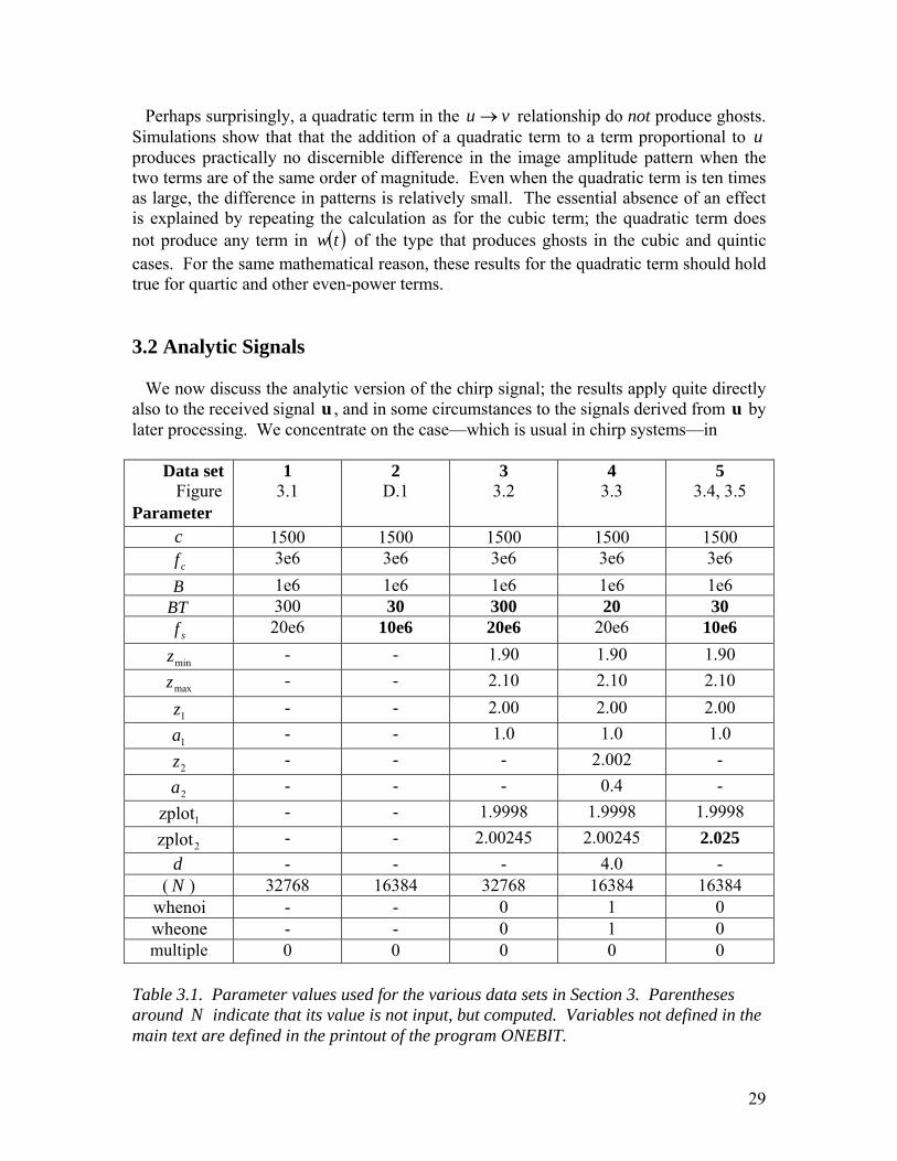
Data set Figure Parameter

1 3.1

2 D.1

3 3.2

4 3.3

5 3.4, 3.5

c 1500 1500 1500 1500 1500 cf 3e6 3e6 3e6 3e6 3e6

B 1e6 1e6 1e6 1e6 1e6 BT 300 30 300 20 30

sf 20e6 10e6 20e6 20e6 10e6

minz - - 1.90 1.90 1.90

maxz - - 2.10 2.10 2.10

1z - - 2.00 2.00 2.00

1a - - 1.0 1.0 1.0

2z - - - 2.002 -

2a - - - 0.4 -

1zplot - - 1.9998 1.9998 1.9998

2zplot - - 2.00245 2.00245 2.025 d - - - 4.0 -

( ) N 32768 16384 32768 16384 16384 whenoi - - 0 1 0 wheone - - 0 1 0 multiple 0 0 0 0 0

Table 3.1. Parameter values used for the various data sets in Section 3. Parentheses around indicate that its value is not input, but computed. Variables not defined in the main text are defined in the printout of the program ONEBIT.

N

29

which the instantaneous frequency (Eqn 2.3) changes by only a small fraction of itself in one cycle (say in the time

if

cf1 ); the condition for this is TfB c

2<< Note at this point that, since necessarily cfB 2≤ , a sufficient condition for the displayed inequality to hold is that

1>>Tfc (3.2) that is, the chirp contains many cycles. Under either of the above two conditions, locally the chirp signal s resembles a monofrequency wave and we expect, to a good approximation, that the quadrature signal is simply the in-phase signal but phase-shifted by 90°. An exception should occur near each end of the chirp. These expectations are borne out by computation. A run was carried out with what might be regarded as typical values of the parameters, given as data set 1 in Table 3.1. Then Figure 3.1 shows the in-phase chirp s and the quadrature part , near the end of the chirp. Away from the end (

is0tt = ) of the chirp, on the ‘inner’ side the phase

difference settles down towards 90°, while on the ‘outer’ side tends to zero. These two ‘adjustments’ made by the curve as the time moves away from the chirp end occur in a time of order one cycle—a time normally very brief compared with the chirp duration.

is

Figure 3.1. The in-phase and quadrature parts of the chirp, near its right-hand end, for data set 1.

30

We briefly studied the behaviour of as it falls off towards zero on the ‘outer’ side (details in Appendix D). It is found that in some circumstances, but not all, tends to zero asymptotically in proportion to

isis

( ) 10

−− tt . In Section 2.3 it was argued that the use of the analytic signal eliminates the ‘fast’ oscillations in . Data sets 3 and 4 (Table 3.1) are used to illustrate this result.( )zp car 10 Data set 3 considers a simple case, while data set 4 involves two targets, considerable noise and one-bit digitisation. The results for the scaled11 image amplitudes are shown in Figures 3.2 and 3.3 respectively. There ( )zp car and ( )zp (Sections 2.2, 2.3) are shown on the same graph. The graphs illustrate the fact (Section 2.3) that is the envelope of . The image is essentially the envelope

( )zp( )zp car ( )zp car ( )zp multiplied by a fast-

oscillation sine curve. Note from Figure 3.2 that the image ( )zp of a single target consists of a main lobe, centred on the target, plus range sidelobes. Of course, in each rapid oscillation, the curve for ( )zpcar normally fails to meet the

curve, because and ( )zp carp p have been evaluated only at discrete points. If the sampling were continuous, the curves in the two figures would be continuous and the envelope relationship would be clearly seen. (A similar remark applies to the ‘ 2π phase shift’ relationship in Figure 3.1.) Actually, one can get rid of these unfortunate effects of discreteness. Since the signal is band-limited and the sampling frequency satisfies the Nyquist relation, one is justified in using FFT interpolation12 to fill in the curves for ( )zp and between the discrete points. ( )zpcar

3.3 Autocorrelation Function and a Continuous-Time Approximation The normalised autocorrelation function of the analytic chirp is defined as as

( ) aa5

a 1 ssy ⊗= ∗K (3.3) where the constant is chosen so that the value of at 5K ay 1=j (or equivalently at

) is unity. (In fact, Eqn 3.3 defines the normalised autocorrelation function of any vector, being replaced by that vector.) To an excellent approximation we have

. (This result is obtained by assuming that the distribution of the phases of the cosine in Eqn 2.1 is approximately uniform and that the quadrature term is

0=tas

TfMK s==5

10 The parameter, wheone, for example, means ‘whether one-bit digitisation is applied.’ 11 In Figures 3.2 and 3.3, a normalisation factor has been introduced such that (not ( )zp ( )zp car ) has a maximum value over equal to unity. In some cases (e.g. Fig. 3.3) the maximum occurs at a value of outside the plotted interval.

zz

12 Thus, to interpolate , one ‘pads’ ( )twa ( )fW a with zeros beyond 2sf± so that that vector contains not but points, where N MN M is some power of two. One then takes the inverse FFT to obtain defined on a finer grid. ( )twa

31

obtained simply by performing a phase shift of 90°.). In the case of E sampling (Section 2.1), due to the linearity of all the operations involved, ( )twa and the complex image amplitude are each a linear combination of versions of the autocorrelation function (3.3). For future use, we note that when time is treated as continuous, Equation (3.3) is transformed into

( )zp a

( ) ( ) ( ) tdttstsT

ty ′+′′= ∫ ∗ aaa 1 (3.4)

At this point we recall the following well-known result (Rihaczek, 1985). A simple formula is obtained for when one makes the following two assumptions: first, that the signal is continuous in time, and second, that the quadrature component is obtained from s simply by replacing ‘cos’ by ‘sin’ in Equation (2.1). The result is

( )ty a

is

( ) ( ) ( )[ ] ( )

Tt

TttfitbT

tTtbtrty c

≥≡

<−

≡=

0

2expsina π

ππ

(3.5)

The long expression on the right-hand side can also be written as ( )[ ] ( tfi

tBTttB

cππ

π2exp

1sin − ) (3.6)

For E sampling, therefore, when the approximation (3.5) is good, and are each a linear combination of functions of the form

( )twa ( )zpa

( )⋅r . Indeed, from Equations 2.4, 2.21, and 3.3 to 3.5, and the fact that now uvq == , we have

( ) ( )∑ −−=i ii

a zctratw 12 (3.7) Then from (2.27), we have for the complex image amplitude

( ) ( )[ ]ii i zzcrazp −= −∑ 1a 2 (3.8)

and is the absolute value of this. For a single target (( )zp 1=i ), the latter quantity is given simply by

( ) ( )[ ]11

1 2 zzcrazp −= − ; (3.9) the carrier wave factor in (3.5) drops out. The approximation (3.5) was tested, first, by considering the case of a single target with E sampling; data set 5 in Table 3.1 is used. The computed image amplitude is compared with the prediction given by the right-hand side of (3.9). The two image amplitude functions are plotted in Figure 3.4, while Figure 3.5 shows the difference plotted on a much expanded scale. (Before any plotting, both amplitude functions have been normalised to have a maximum value of unity.) In one sense the agreement is excellent: the maximum absolute error is just 0.4% of the maximum value. The relative error is less good, but is still satisfactory. Thus the error at range , relative to the nearest sidelobe peak, reaches a maximum value of 17%; but is much better than 17% in the nearer sidelobes.

z

32

Figure 3.2. Two image amplitude functions, ( )zp car and , that are alternative images generated from data set 3 (

( )zp=z range). The target is at z =

2.000 m.

Figure 3.3. As for Figure 3.2, but for data set 4. The targets are at z = 2.000 and 2.002 m.

33

We can describe the difference between two image amplitude functions by measures other than the maximum difference. Such measures are defined in Appendix E. In the present case they are measures of the error introduced by the continuous-time approximation, and they are found (Appendix E) to be small. A similar calculation in the appendix shows that Equation (3.5) is good also in respect of the carrier wave. (One must beware, however, that these are measures of absolute, not relative difference, in the sense defined in the previous paragraph.) The carrier wave becomes important when two or more targets are present, since, in Equation (3.8), complex numbers are added. As a further check on the continuous-time approximation, a test was carried out as in the paragraph before last, but for a scene with two targets. A level of agreement is found similar to that in the one-target case. We recall that the first assumption on which Equation (3.5) is based is that the sampling is continuous. But in the present results, since the sampling frequency used, 10 MHz, is not all that much greater than the central frequency (3 MHz), there are only about three sample points per cycle, so that the sampling is nowhere near continuous. We conclude that, after all, it is not a required condition of validity that many samples be taken per cycle. (The Nyquist condition must, however, be satisfied.) It therefore appears that, of the two assumptions that led to (3.5), only the second (that the quadrature component is obtained by replacing cos by sin) produces an appreciable error.13 Furthermore that error should be small provided that the chirp contains many cycles (see Eqn 3.2). Finally, then, we conclude that the continuous-time predictions, (3.7) to (3.9), are good approximations provided that the chirp contains many cycles. 3.3.1 Constructive and Destructive Interference In succeeding sections we shall often be concerned with a system containing a strong target (the ‘first’ target) and a weak (second) target at . Of interest is the question of whether the sidelobe (at ) from the strong target interferes constructively or destructively (or something in between) with the main lobe of the weak target. Three factors contribute to the answer, represented by the numbers , and as follows. Let be the separation of the two targets. First, the carrier wave factor

2z

2z

1m 2m 3mzΔ ( )tfi cπ2exp in

(3.5) has an effect represented by the number ( )41 λzm Δ= , where λ is the wavelength at the central frequency. (In obtaining this result, the usual association ( ) tcz Δ=Δ 2 is made.) Secondly, the phase of the sine in (3.5) affects the sign of ( )tr ; this is represented by that integer such that the phase lies in the interval 2m ( )( )ππ 1, 22 +mm ( is the usual sidelobe number). Thirdly, the target strengths, and , may differ in sign. Let

be zero if the signs are the same, one if different. Then constructive or destructive interference occurs according as

2m

1a 2a

3m

321 mmm ++ is even or odd. 13 There is therefore a case for calling the approximation that leads to Equation (3.5) as the ‘cos-to-sin approximation’ rather than the ‘continuous-time approximation.’

34

Figure 3.4. Comparison of the prediction (3.9) with the image obtained for the E-sampling data set 5. As the curves are symmetric about the target position ( , the left-hand half has not been plotted. )2=z

Figure 3.5. As for Figure 3.4 except as follows. The dashed curve now plots, on an expanded scale, the difference of the image amplitude from the prediction (expansion factor ). 200=

35

4. Relinearisation; Image Noise Model 4.1 Relinearisation: Analytical We recall that, at any discrete time, the output from the one-bit digitiser is not a linear function of u . In general this leads to ‘ghost’ images. Section 1.2 stated a pair of results, according to which, under certain circumstances, effectively the linearity is restored. We now justify those results.

v

4.1.1 Linearity in the Mean (LIM) At each value of , given the value of t ( )tu , ( )tv follows a probability distribution due to the distribution of noise values, assumed to be the uniform distribution (2.9). Consider first the case where . A simple calculation using (2.8), (2.9) and (2.11) shows that the distribution of v is

dud ≤≤−

( )

( ) ⎟⎠⎞

⎜⎝⎛ +=+=

⎟⎠⎞

⎜⎝⎛ −=−=

dudv

dudv

1Pr

1Pr

21

21

(4.1)

It follows that the mean, root-mean-square value and standard deviation of v are ( ) ( ) 2122

rms , , udvdvuv −=== σ (4.2) Secondly and thirdly, consider the cases du −< and : then the probability is one that equals and respectively; accordingly the mean also is and

du >v d− d+ d− d+

respectively, while the standard deviation is zero. Therefore the mean of v , as a function of , is given by the piecewise linear graph of Figure 1.1. The reason for inserting the factor in (2.11) is now clear: the simple result (4.2) for the mean then requires no constant of proportionality.

ud

Let be the maximum, over time, of the absolute value of maxu ( )tu ; and consider the case

maxud ≥ (4.3) Then the results (4.2) hold for all possible u . Thus, under the condition (4.3), the mean of is linear in . Also the constant of proportionality, unity, is independent of the

index jv ju

j . Consider the vectors w and p . Let w denote the expectation value over an

ensemble of values of the noise stream , and similarly for n p . Such an average is carried out for each value of the discrete time, in the case of ; or for each value of , in the case of . Since the vector is a linear function of the vector , from (2.12) and (2.13), it is also true that

w zp w v

w (and trivially also v ) is a linear function of u . Furthermore, since the image amplitude ( )zp is simply evaluated throughout at

, w

zct 12 −= p is likewise a linear function of u . Indeed the functional dependence of

36

p , w and v on u is the same as in the corresponding E-sampling case. While the

above results have been stated for p , w and v , clearly the same arguments may be

invoked to show that the corresponding results hold also for the analytic signals, ap , aw and av . Thus we have proved that, under the condition (4.3), the system is

linear in the mean. It was found earlier that Equations (3.7) to (3.9), given by the continuous-time approximation, hold when E sampling is employed. It now follows that Equations (3.7) to (3.9) continue to hold when O-sampling is performed, provided that the quantity on each left-hand side is replaced by its expectation value. Thus we have, for example,

( ) ( )[ ]ii i zzcrazp −= −∑ 1a 2 (4.4) The conditions required are that the chirp contains many cycles and that the condition (4.3) is satisfied. Note, from (4.4) together with (3.5) without the carrier wave factor, that the contribution to this mean profile from each target consists of a main lobe plus range sidelobes. Note that (4.4) refers to the mean of the complex image amplitude; the mean of itself does not in general obey such a simple formula. ( )zp 4.1.2 LIM: Signal-to-Noise Ratio Consider the values of consistent with (exact) linearity in the mean, that is, . The sequence contains a ‘signal’ component

d maxud ≥

jv uv = together with a ‘noise’

component vv − . At a sampling time at which u has a given value, the noise

component has rms value ( ) ( ) 2122 udv −=σ . For any given u , the signal-to-noise ratio (SNR) is

( )

12

2

2

1 1SNR−

⎥⎥⎦

⎤

⎢⎢⎣

⎡−⎟

⎠⎞

⎜⎝⎛==

ud

vv

σ (4.5)

As rises from to higher values, decreases. Therefore the optimum noise level is the minimum value allowed by (4.3), namely

d maxu 1SNR

maxud = . Rather than quote a signal-to-noise ratio for each u , for most purposes it is desirable to quote an overall SNR—a ratio that involves weighted averages over the values of u . As a first attempt, we note that a rough measure for the SNR is obtained by considering , a typical value of . Inserting for u in Equation (4.5), we obtain

typuu typu

12

typ2 1SNR

−

⎥⎥

⎦

⎤

⎢⎢

⎣

⎡−⎟

⎟⎠

⎞⎜⎜⎝

⎛=

ud (4.6)

37

as a rough overall measure of the SNR. Since is independent of , this formula provides a reasonable basis for discussing the dependence of the overall SNR on . For the case , the formula (4.6) becomes

typu dd

typud >>

( )2typ2SNR du= (4.7)

This shows that setting to a large value incurs a large penalty in the SNR. d We can go some way towards pinning down the value of . For the case of one

target, note, first, from (2.4), that typu

1max au = ; therefore, in any one-target formula below,

we are free to replace by maxu 1a . For one target, a reasonable choice is

2maxtyp uu = since this is the rms value of u for the case where noise is added only over the duration T of the proper part of the returning chirp. The case of many targets is discussed below in Section 4.1.4. In situations where it is possible to write a formula for the distribution of the u values that occur in the time-interval during which noise is injected (as a probability density function ) a unique expression for the overall signal-to-noise ratio—to be called

—can be written down. Thus ( )uPr

3SNRNS=3SNR (4.8)

where ( )

( ) ( ) ( ) ( )duuudduuvN

duuuS

PrPr

Pr222

2

∫∫∫

−==

=

σ (4.9)

where (4.2) has been used. Such a situation occurs when there is a single target (and noise is added only over the duration T of the proper chirp). (Unfortunately a single point target is not typical of UAI!) Since the signal ( )tu is essentially sinusoidal, we have

( ) ( ) maxmax2122

max1 Pr uuuuuu ≤≤−−=

−−π (4.10) and, using (4.9),

2max2

122max2

1 , udNuS −== (4.11)

We thus obtain 12

max3 12SNR

−

⎥⎥⎦

⎤

⎢⎢⎣

⎡−⎟⎟

⎠

⎞⎜⎜⎝

⎛=

ud (4.12)

where, as discussed above, for we may substitute maxu 1a . (Note that Eqns 4.6 and 4.12 happen to agree when is put equal to the rms value of u .) typu

38

Table 4.1 shows the values of for selected values of the noise level . It is seen that when d rises from to , already there is a considerable SNR penalty.

3SNR d

maxu max2u

maxud 1 2 3 10

3SNR 1 0.143 0.0588 0.00503

Table 4.1. Signal-to-noise ratios, , for a system containing one target. 3SNR

4.1.3 An Upper Limit on maxu We can obtain an upper limit on , determined by the chirp duration T , the strengths of the targets and their approximate positions. In the sum (2.4) for , at each time t only some of the targets contribute, because each target contributes only for a time

. (We ignore the tail of the chirp’s quadrature part.) Indeed, the time axis can be subdivided in a unique way into intervals J such that the set of contributing targets remains constant throughout each interval but changes at the ends of the interval. Each such interval will be called a constant-strength interval. Let

maxu( )tu

T

( )JT be the set of targets that contribute in the interval J. Then let

( )∑∈

=JTJMAX max

iiau

Then from (2.1) and (2.4), we have MAXmax uu ≤ ; (4.13)

and so, from (4.3), a sufficient condition for LIM is MAXud ≤ (4.14)

maxu equals in the special case where, at some time in the maximising interval J, the returns from all the targets in are in phase with each other.

MAXu( )JT

4.1.4 Typical Signal Level u in a Constant-Strength Interval Let us consider a constant-strength interval J in which many targets contribute. Then the rms value of , for , satisfies ( )tu J∈t

( )∑∈

=JT

2212

rmsJi

iau

Here, in the return signal from each target, the mean of the cosine-squared resulting from Equation (2.1) has been put equal to one-half and the cross-terms have been put equal to zero. This should be satisfactory provided that the placement of the targets is random, in the sense that there are no marked constructive or destructive interference effects when the returns from the various targets are combined. Then may be taken as typical of

the values of rmsJu

( )tu for ; thus J∈t

rmsJtyp uu =

39

Let us now suppose that the sum of the in the display equation is not dominated by one or a few targets. Then, by the central limit theorem, to at least a rough approximation, in J, the values of

2ia

( )tu follow a normal distribution with mean zero and standard deviation . rmsJu We return to the question of what value of is to be used in the equation, (4.6), that

gives the measure . We saw in Section 4.1.2 that for one target, typu

2SNR 2maxtyp uu = . For many targets, let us suppose that the conditions that led to the normal distribution of

values hold. Then, first, it is clear that is now divided by a much larger

number than

( )tu typu maxu

2 (since the returns from the various targets have essentially random relative phases when combining to produce , but tend more to have identical phases when combining to produce ). Second, and more specifically, for any constant-strength interval J, it is appropriate, in the equation (4.6) for , to use the value

(given in turn by the display equation above).

typu

maxu

2SNRrmsJtyp uu =

4.1.5 Effective Value of maxu Consider the case where there are many targets and the other conditions that led to the normal distribution in Section 4.1.4 hold. In the context of the uniform noise distribution, the condition is then unduly restrictive, as approximate linearity in the mean should be sufficient for the production of good images. For, in the many-target case, there are possible values of u that occur only when the contributions from many targets add in phase with one another; yet these values of occur only rarely.

maxud ≥

u Let be the interval J for which 1J

( )∑∈ JT

2

iia is a maximum, and let us write .

We expect that, in the condition (4.3), in practice, can be replaced by an effective value, , such that, for ,

rmsJrms1 1uu =

maxu

maxeu 1J∈t ( )tu exceeds in no more than of the samples, where , say. The properties of the normal distribution then yield

maxeu %p%5=p

rms 1max e uu θ= where 2≈θ . (To deal with situations where the assumptions for a normal distribution do not hold all that well, it would be reasonable to raise θ to 2.5 or 3.) The resulting relaxed criterion,

max eud ≥ , should produce, at most, occasional or weak ghost images.

40

4.1.6 Non-Uniform Distribution of Noise We now consider the case where the uniform distribution (2.9) of the noise voltage is replaced by a general probability density function. Then in place of (4.1) we have

( ) ( ) dnndvu∫∞

−

=+= PrPr (4.15)

In Figure 1.1(iii), the resulting dependence on v on is shown for a normal distribution. Note that the curve is linear near the origin. We shall derive a result that makes use of this fact.

u

Suppose that is an even function of , behaves smoothly near and has an rms value

( )nPr n 0=nσ that is finite—for example, the normal distribution. Then, as the ratio

maxuσ becomes large, in Equation (4.15), the range of integration can be subdivided into the intervals and ; and in the former we may put ( 0,u− ) )( ∞,0 ( ) ( 0PrPr =≈ nn ) for all permitted u . Thus we have

( ) ( )[ ] undv 0PrPr2

1 =+=+=

It follows that the mean of becomes a linear function of : v u( )[ ] undv 0Pr2 == (4.16)

but only asymptotically as the noise level σ becomes large compared to . Indeed in this limit, not only the first but the second and third of the italicised results in Section 4.1.1, below (4.3), hold.

maxu

4.1.7 Full Linearity Linearity in the mean is not by itself sufficient to produce a linear system, as there are fluctuations about the mean. However, the signal is produced from , essentially by the cross-correlation process, (2.13) or (2.21). If the chirp is very long, any interval

w v

( uuu )δ+, is sampled many times; in the calculation of w , effectively there is averaging over these sample points. As a result, at any t , ( )tw should be close to the value obtained by putting equal to v v in (2.13). Thus to a good approximation, if the chirp is very long, under the condition (4.3), the IC system together with the cross-correlator should be fully linear and there should be no ghosts. (The result, that the system is linear if ‘the noise exceeds the received signal,’ has been stated in words by David Robinson, private communication; his conclusion draws on the work of Gammaitoni, 1995.) For a chirp of finite length, , and hence ( )tw ( )zp a , will fluctuate to some degree about the mean value (4.4). Thus there are fluctuations in both ( )zp a and , which we shall call image noise.

( )zp

41

4.2 Image Noise Model: Description Later (in Section 6) we shall be discussing simulations in which necessarily, due to the finite chirp length, there is image noise. In order to be ready to discuss the simulated results in a systematic way, it is useful to propose and test a model for that image noise. This, the image noise model, is the subject of the present subsection. By definition, the (complex) image noise is

( ) ( ) ( )zpzpzp aaan −= (4.17)

where the average is over an ensemble of noise streams n at fixed . The image noise is zero for E sampling and will be called O noise for O sampling. The image noise of the complex amplitude has expectation value zero. Defining the (real) image noise as

z

ann pp = , we note that

( ) ( )2an

2an

2an

2n ImRe pppp +==

where Re means real part. Defining ( )rmsanp to be the square root of the term between the

two equality signs, we have that the root-mean-square O noise ( )rmsnp satisfies

( ) ( ) ( ) ( ) 21

2rms

an

2rms

an

2rms

an

2rmsn ImRe τ=+≡= pppp (4.18)

where the rightmost equality defines 1τ . Note that (4.18) holds even if there is a correlation between the real and the imaginary parts. The model consists of four assumptions as follows.

1. (i) For each , the real and imaginary parts of z ( )zp an follow a joint normal

distribution.

(ii) There is no correlation between the real and the imaginary parts.

(iii) The two parts have the same root-mean-square value as each other (equal to 21τ , from Eqn 4.18).

2. 1τ is independent of (irrespective of the target positions). (There may be, and in fact there is, a correlation between the values of

z( )zp a

n for two different values.) z

3. (i) 1τ is proportional to d and also to T1 .

(ii) At constant B , 1τ is proportional to sf1 but is independent of . cf

(iii) At constant , and sf cf T , 1τ is independent of B .

4. 1τ does not depend on the set of target strengths.

It will usually be further assumed that ( )zp a is given by the continuous-time prediction, Equation (4.4). As stated, this should be a good approximation provided that the chirp contains many cycles and ( or) . maxud ≥ max eud ≥

42

We argue for the proportionality to T1 as follows. The cross-correlation (2.21) produces a kind of average over TfM s= samples, and so, since the number of data in the average is proportional to T , the O noise, relative to the ‘signal’ (which is

independent of T ), should vary in proportion to

( )zpμ

T1 . By the same argument, the proportionality to sf1 should hold. Independence of is expected because appears to act only as a ‘carrier wave frequency’; changing does not change the number of samples. The proportionality to is very plausible but we do not present an argument, relying instead on numerical tests.

cf cf

cfd

The independence of B then follows from a dimensional argument. For we now have

TfEd s=1τ (4.19)

where E is dimensionless. E therefore cannot be a power of B (except 0B ). In addition, E cannot be a power of sfB , cfB or BT , else either assumption 3(i) or assumption 3(ii) would be violated. Hence14 the result 3(iii). 4.3 Image Noise Model: Tests In this subsection a partial testing of the image noise model is carried out, to give a sufficient degree of confidence in the model to justify its use in a different investigation in Section 6. 4.3.1 Initial Tests The initial testing was done by using data sets 6 to 8 in Table 4.2. Data set 6 uses a single target, a noise amplitude nearly as low as the condition (4.3) allows and quite a long chirp ( ). The two values just mentioned ( and

d300=BT d BT ) are chosen with the

aim of making the O noise low (compared even to the first sidelobe). The results (for a particular noise stream) are shown in Figures 4.1 and 4.2. In these and subsequent figures, we use the definition

( )pred

amean' predicted' zp= (4.20)

where pred means ‘predicted by the continuous-time approximation (and thus given by Equation 4.4 supplemented by Equation 3.5).’ Quotation marks are placed around ‘predicted mean,’ partly because of continuous time, but more importantly, because the quantity is not the mean of the real ( )zp , but the absolute value of the mean of the complex . Figure 4.1 shows that the O noise has little effect on the main lobe and ( )zp

14 One could object that 1τ could depend on B in a more complex way, via the combination

, where is the position of the strongest target. But this is ruled out by assumption 2.

( 11 zzBc −− ) 1z

43

has no qualitative effect on the first few sidelobes, but has a dominating effect on the distant sidelobes. The results are consistent with an O noise level that is independent of

and lies below, but not too far below, the main lobe level of the ‘predicted mean.’ z Data set Figure Parameter

6 4.1–4.3

7 -

8 -

9 4.4–4.5

10 4.6

11 4.7

c 1500 1500 1500 1500 1500 1500

cf 3e6 3e6 3e6 3e6 3e6 3e6 B 1e6 1e6 1e6 1e6 1e6 1e6

BT 300 300 30 300 300 30 sf 20e6 20e6 20e6 20e6 20e6 20e6

minz 1.90 1.90 1.90 1.90 1.90 1.90

maxz 2.10 2.10 2.10 2.10 2.10 2.10

1z 2.00 2.00 2.00 2.00 2.00 2.00

1a 1.0 1.0 1.0 1.0 1.0 1.0

2z - - - 2.0025416 2.0025416 2.0025416

2a - - - 0.50 0.50 0.50

1zplot 1.995 1.995 1.995 1.995 1.995 1.995

2zplot 2.015 2.015 2.015 2.015 2.015 2.015 d 1.5 4.5 1.5 1.5 4.5 1.5

( ) N 32768 32768 16384 32768 32768 16384 whenoi 1 1 1 1 1 1 wheone 1 1 1 1 1 1 multiple 0 0 0 0 0 0

Table 4.2. Parameters values used for data sets 6 to 11. To study the O noise directly, the quantity

( ) ( )pred

aanoise' O' zpzp −= (4.21)

(note the inclusion of quotation marks) was computed15 for each and the results plotted on an expanded scale in Figure 4.2. Note that in (4.21) complex, not real, quantities are computed and subtracted. (Note the quotation marks, used to signify the precise expression on the right-hand side.)

z

16 Figure 4.2 gives an overall impression that the O noise level is independent of , in accordance with assumption 2. z

15 To see how to compute ‘O noise’ using ONEBIT, find ‘O noise’ among the comments in ONEBIT. 16 becomes equal to the ‘O noise’ if the continuous-time approximation is invoked. ( )zpn

44

Figure 4.1. Image amplitudes for data set 6. A single target. The ‘predicted mean’ is defined in the text. The solid curve results from O sampling.

Figure 4.2. Uses the same complex image amplitudes as led to Figure 4.1 (data set 6). It plots the ‘O noise’ defined in the text, plotted with expansion factor 10.=

45

Figure 4.3. As for Figure 4.2, only a different noise stream is used. Data set 6 is still being used.

Figure 4.4. Image amplitudes from data set 9. There is a second, weaker target at . m 0025416.2=z

46

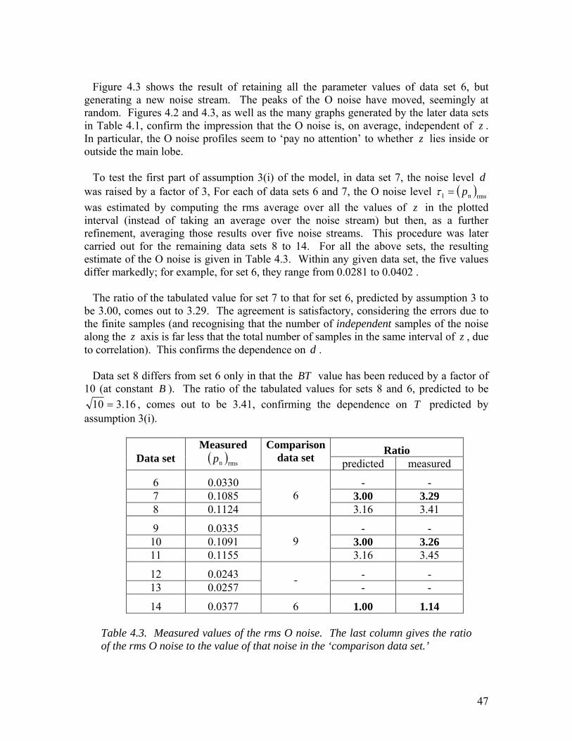
Figure 4.3 shows the result of retaining all the parameter values of data set 6, but generating a new noise stream. The peaks of the O noise have moved, seemingly at random. Figures 4.2 and 4.3, as well as the many graphs generated by the later data sets in Table 4.1, confirm the impression that the O noise is, on average, independent of . In particular, the O noise profiles seem to ‘pay no attention’ to whether lies inside or outside the main lobe.

zz

To test the first part of assumption 3(i) of the model, in data set 7, the noise level was raised by a factor of 3, For each of data sets 6 and 7, the O noise level

d( )rmsn1 p=τ

was estimated by computing the rms average over all the values of in the plotted interval (instead of taking an average over the noise stream) but then, as a further refinement, averaging those results over five noise streams. This procedure was later carried out for the remaining data sets 8 to 14. For all the above sets, the resulting estimate of the O noise is given in Table 4.3. Within any given data set, the five values differ markedly; for example, for set 6, they range from 0.0281 to 0.0402 .

z

The ratio of the tabulated value for set 7 to that for set 6, predicted by assumption 3 to be 3.00, comes out to 3.29. The agreement is satisfactory, considering the errors due to the finite samples (and recognising that the number of independent samples of the noise along the axis is far less that the total number of samples in the same interval of , due to correlation). This confirms the dependence on .

z zd

Data set 8 differs from set 6 only in that the BT value has been reduced by a factor of 10 (at constant B ). The ratio of the tabulated values for sets 8 and 6, predicted to be

16.310 = , comes out to be 3.41, confirming the dependence on T predicted by assumption 3(i).

Ratio Data set

Measured ( )rmsnp

Comparison data set predicted measured

6 0.0330 - - 7 0.1085 3.00 3.29 8 0.1124

6 3.16 3.41

9 0.0335 - - 10 0.1091 3.00 3.26 11 0.1155

9 3.16 3.45

12 0.0243 - - 13 0.0257

- - -

14 0.0377 6 1.00 1.14

Table 4.3. Measured values of the rms O noise. The last column gives the ratio of the rms O noise to the value of that noise in the ‘comparison data set.’

47

Figure 4.5. Uses the same complex image amplitudes that led to Figure 4.4 (data set 9). Two targets. Expansion factor = 10.

Figure 4.6. Results for data set 10. Two targets. Expansion factor = 3.

48

Figure 4.7. Results for data set 11. Two targets. Expansion factor = 3.

Figure 4.8. Results for data set 13; two targets. The ‘predicted mean’ contributions from the two targets interfere destructively at the weaker target (located at the vertical line).

49

Figure 4.9. Uses the same complex image amplitudes as led to Figure 4.8 (data set 13). The figure shows the ‘O noise,’ plotted with expansion factor = 10.

Figure 4.10. Results from data set 15, to determine the extent of O noise. The dashed vertical line is at the upper limit in (4.24) and the dotted vertical line is at

. The ‘predicted mean’ curve is cut off at a height of 0.6. Expansion factor = 2.

maxz

50

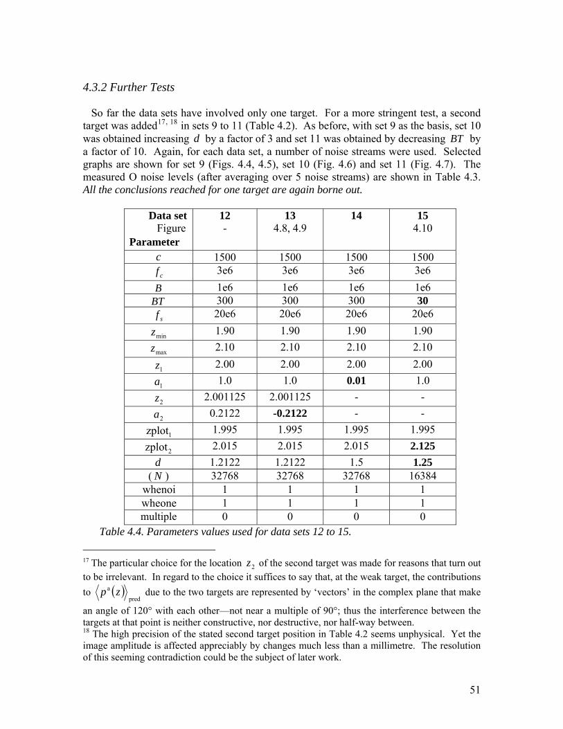
4.3.2 Further Tests So far the data sets have involved only one target. For a more stringent test, a second target was added17, 18 in sets 9 to 11 (Table 4.2). As before, with set 9 as the basis, set 10 was obtained increasing by a factor of 3 and set 11 was obtained by decreasing d BT by a factor of 10. Again, for each data set, a number of noise streams were used. Selected graphs are shown for set 9 (Figs. 4.4, 4.5), set 10 (Fig. 4.6) and set 11 (Fig. 4.7). The measured O noise levels (after averaging over 5 noise streams) are shown in Table 4.3. All the conclusions reached for one target are again borne out.

Data set Figure Parameter

12 -

13 4.8, 4.9

14 15 4.10

c 1500 1500 1500 1500 cf 3e6 3e6 3e6 3e6

B 1e6 1e6 1e6 1e6 BT 300 300 300 30

sf 20e6 20e6 20e6 20e6

minz 1.90 1.90 1.90 1.90

maxz 2.10 2.10 2.10 2.10

1z 2.00 2.00 2.00 2.00

1a 1.0 1.0 0.01 1.0

2z 2.001125 2.001125 - -

2a 0.2122 -0.2122 - -

1zplot 1.995 1.995 1.995 1.995

2zplot 2.015 2.015 2.015 2.125 d 1.2122 1.2122 1.5 1.25

( ) N 32768 32768 32768 16384 whenoi 1 1 1 1 wheone 1 1 1 1 multiple 0 0 0 0

Table 4.4. Parameters values used for data sets 12 to 15. 17 The particular choice for the location of the second target was made for reasons that turn out to be irrelevant. In regard to the choice it suffices to say that, at the weak target, the contributions to

2z

( )pred

a zp due to the two targets are represented by ‘vectors’ in the complex plane that make

an angle of 120° with each other—not near a multiple of 90°; thus the interference between the targets at that point is neither constructive, nor destructive, nor half-way between. 18 The high precision of the stated second target position in Table 4.2 seems unphysical. Yet the image amplitude is affected appreciably by changes much less than a millimetre. The resolution of this seeming contradiction could be the subject of later work.

51

In producing the ‘predicted mean’ image amplitude at the position of the weak target, the contributions of the two targets may interfere constructively or destructively (see Section 3.3.1). It was decided to test the model under these ‘extreme’ conditions, via data sets 12 and 13 (Table 4.4). The second target was placed at the first sidelobe peak of the strong target (a position that happens to give constructive or destructive interference). Its strength was chosen so that, at that point, either the two contributions to

pred

ap are

equal (set 12) or one is the negative of the other (set 13, note the changed sign of ). was chosen as small as allowed by Equation (4.3).

2a d

The results from one of the runs with set 13 are shown in Figure 4.8; the difference or ‘O noise’ is plotted explicitly in Figure 4.9. In Figure 4.8, the image amplitude curve follows the undulations of the ‘predicted mean’ curve for the first few sidelobes—as in Figure 4.1. It should be noted that there is a very low value of ( )zp at the weak target’s position—as there should be, due to the destructive interference. Importantly,

( ) ( )zpzp ann = does not rise to an anomalously high value at this point.

Figures 4.8 and 4.9, taken together, show that the image amplitude tracks the predicted mean curve fairly closely in those intervals of where the mean is considerably above the O noise. Despite the changed shape of the ‘predicted mean’ curve, the O noise seems to be independent of , on average, apparently ‘paying no attention’ to whether lies in a high lobe—again in accordance with assumption 2.

z

z z

To test assumption 4, seven runs were carried out using data set 14 (Table 4.4), differing from set 6 only in that is changed from 1.00 to 0.01; is kept unchanged. As shown in Table 4.3, the resulting ratio of the two values of

1a d

1τ is 1.14, in satisfactory agreement with the prediction of 1.00. 4.3.3 Formula for O Noise At the end of Section 4.2 a formula for the rms O noise, 1τ , was derived; however, it contains an unknown dimensionless constant E , which we now estimate. For each of the data sets 6 to 14, from the estimate of 1τ given above, a preliminary estimate of E is calculated; the results are given in Table 4.5. The simple average of these nine estimates is then taken to yield the final estimate 783.1=E . The investigations therefore indicate that the rms O noise is given, under very general conditions, by

Tfd s78.11 =τ (4.22) The conditions are that the chirp contains many cycles and . max eud ≥

52

Data set Estimate of E Data set Estimate of E

6 1.704 11 1.886 7 1.868 12 1.553 8 1.835 13 1.642 9 1.730 14 1.947 10 1.878 Mean 1.783

Table 4.5. Estimation of the numerical coefficient E in the formula for rms O noise.

4.3.4 Extent of O Noise Up to this point we have not considered how far the O noise extends in range; this will now be rectified. We saw in Section 2 that noise is added only at the times lying between

and , where the latter are given by Equation (2.10). We shall estimate the effect on the O noise by ignoring the one-bit step in the processing and supposing, instead, that the noise simply adds to the signal

neart fart

( )tn ( )tu to produce ( )tv . (Of course, any O noise calculated on the basis of this procedure does not have significance by itself; significance attaches to the ratios of two such calculated O noises.) The crucial step in image formation is the crosscorrelation of ( )tv with ( )ts to produce ( )tw (filtering being ignored). Since has length T , for any t in ( )ts

22 farnear TttTt −<<+ ( )tw will receive its ‘full contribution’ from the noise stream ( )tn , unaffected by the

cutoffs (2.10); the O noise will be constant with on average. For lying outside the interval

t t

( )2,2 farnear TtTt +− ( )tw will receive a zero contribution from the noise; the O noise will be zero. Using

(2.10) and the relation ( )tcz 2= (from Eqn 2.16), we have that the O noise is constant throughout the interval

( )maxmin , zz (4.23) of and zero outside z

( 2,2 maxmin cTzcTz )+− (4.24) In between and maxz 2max cTz + , the argument (still based on ignoring the one-bit step) shows19 that the mean-square (not root-mean-square) value of the O noise falls linearly as increases. Thus the rms O noise is predicted to fall towards zero as the square root of the linear expression, and thus trace out a parabola with a horizontal axis. Similar remarks apply near .

z

minz To test these predictions, for the data set 15 (Table 4.4), the O noise is plotted in Figure 4.10. The fall-off from maximum to zero is predicted to occur over the interval 19 Discrete time must be used for this part of the calculation.

53

1225.210.2 << z . The results are consistent with the predictions. (It must be added, however, that the ‘parabola’ relationship has not been strongly tested.) 4.3.5 Conclusion By way of conclusion at this point, the tests have confirmed aspects of the image noise model. This is considered a sufficient basis for using the model in Section 6, where the model is relied on only weakly while a different matter is investigated. It is intended, in future work, to test each of the three subassumptions of assumption 1 (the normal distribution with certain properties) and to test more thoroughly assumption 2 (that statistically, the noise is independent of ) and assumptions 3 and 4. The testing of the three subassumptions, could be done by considering one or more individual values of and performing computations over many noise streams. Independence of could be tested in the same way, but would require several values to be considered. However, instead of a numerical approach, it is intended, if possible, to use an analytical approach, such as was used in Section 4.1, since this may well answer the relevant questions with relatively little work.

zz

zz

5. Power Spectra; Filtering 5.1 Power Spectra In this subsection, power spectra of the signals , , and are presented and discussed. Some preliminary remarks are appropriate. The spectra chosen for presentation are shown in Figures 5.1 to 5.4. The part of the spectrum running from frequency to

u n v w

0=f 2sff = essentially gives the complete spectrum; for the in-phase signal, the plot from 2sf to is obtained by reflecting the curves about the line sf

2sff = . As in the present data sets, Figures 5.2 and 5.3 give complete spectra. The figures also show the two edges of the nominal band

MHz 20=sf( )2,2 BfBf cc +−

of the chirp. Consider first the E-sampling data set 21 in Table 5.1 ( 0wheonewhenoi == ); the spectra for the signal before cross-correlation and the signal after cross-correlation are shown in Figure 5.1. For a very long chirp, one might expect the spectrum of the received signal

vu = w

( )tu to resemble a rectangle function, the power being concentrated in the nominal band. For the present set, with its medium-length chirp ( ), not surprisingly, the spectrum of the received signal 100=BT ( )tu (dashed curve) has a quite appreciable tail lying outside the band. What may come as a surprise is the rather large oscillations (dashed curve) inside the band. The curve for shows that the cross-correlation has two effects. First, the out-of-band tail is much reduced; the cross-correlation removes much of the power outside the band. And second, inside the band the oscillations are accentuated, becoming very large.

w

54

As a typical example of O sampling, the data set 22A was used; the next two Figures give the smoothed spectra of the noise n (Fig. 5.2) and of the signal v after one-bit sampling (Fig. 5.3) (as well as ). It turns out that, for O sampling, the unsmoothed curves for and v (and indeed ) show oscillations that are large and very rapid, giving graphs with filled-in black regions that are hard to interpret. For this reason a smoothing window of size fwidav (Table 5.1) has been applied to all the spectral curves in these two Figures; that is, the power density at a given frequency has been replaced by the average of the power density values at fwidav consecutive values of centred on the given value.

un w

ff

f The spectrum of the received signal is again displayed in the present two Figures. These plots would be the same as in Figure 5.1, were it not for the fact that smoothing is now applied. Note that the smoothing not only greatly reduces the oscillations in the band; it also widens considerably the ‘step’ at each band edge. Thus the curve for u in these two Figures can only be regarded as schematic. (Similarly, it is believed that the two ‘steps’ in the spectrum of the true v are narrower than they appear in Fig. 5.3.)

u

The spectrum of the noise (Fig. 5.2) is uniform over the whole interval ( )tn ( )2,0 sf , but with fluctuations that depend on the particular noise stream. The unsmoothed spectrum (not shown) behaves similarly except that the fluctuations become much larger—comparable with the average or rms value of the noise itself. The spectrum of the signal v after one-bit sampling (Fig. 5.3), which ideally would be simply the spectrum of , has a very appreciable noisy (ragged) component outside the band and also inside.

u

For presentation purposes, in the production the corresponding curve for , the signal after cross-correlation (Fig. 5.4), changes were made to the ‘plotting’ parameters ( ,

and widav), the result being data set 22B. Thus the frequency range plotted has been narrowed and the window has been reduced from 201 points to 21. Table 5.1 shows that no other changes to the parameters were made; however, a new noise stream was used. It is seen that the cross-correlation ‘removes’ the components of v outside the band, except for rather short tails near the two band edges. The window has been reduced sufficiently so that the ‘step’ in at the edge has been subjected to little widening; the rate of decline of the unsmoothed is represented fairly well.

w1fplot

2fplot

ww

We note also that, inside the band, , like , has a quite noisy component. It is noteworthy that, as the frequency changes, the fluctuations in track quite closely the fluctuations in .

w vw

v 5.2 Filtering From Figure 5.3, the signal ( )tv contains strong frequency components that are well outside the nominal band ( 2,2 BfBf cc )+− —components that are not present in

55

Data set Figures

Parameter

21 5.1

22A 5.2–5.3

22B 5.4

23 5.5, 5.6

c 1500 1500 1500 1500 cf 3e6 3e6 3e6 3e6

B 1e6 1e6 1e6 1e6 BT 100 100 100 30

sf 20.e6 20.e6 20.e6 20.e6

minz 1.995 1.995 1.995 1.995

maxz 2.01 2.01 2.01 2.01

1z 2.00 2.00 2.00 2.00

1a 1 1 1 1

1zplot - - - 1.99

2zplot - - - 2.02 d - 1.5 1.5 1.5

( ) N 16384 16384 16384 16384 whenoi 0 1 1 1 wheone 0 1 1 1 whefil 0 0 0 0; 1

BE - - - 05.12021 = BA - - - 05.0201 =

1fplot 2.001e6 0 2.001e6 -

2fplot 3.999e6 10.e6 3.999.e6 - fwidav 1 201 21 -

multiple 0 0 0 1 idiff - - - 2

Table 5.1. Data sets 21 to 22B, used to obtain power spectra, and 23, used to investigate filtering.

( )tu . Because of this, it has been suggested that the image would be improved if these

components were filtered out. ONEBIT was used to investigate this claim. For this purpose, data set 23 (Table 5.1) was used. To compare the image with filtering to that without filtering, it is necessary effectively to run ONEBIT twice; hence the two values of whefil (whether to filter) in the Table. For a good comparison, it is necessary that the same noise stream be used for the two runs. In ONEBIT this is accomplished by setting the variable, multiple (whether there are multiple runs), equal to one. Note that the data set puts the values of the filter parameters, E and A , equal to the ‘guessed optimum’ values given in Section 2.4. Note also that a shorter chirp ( ) is used for the present test.

30=BT

56

Figure 5.1. Power spectra of (u v= ) and , for data set 21 (E sampling). No smoothing. The two edges of the nominal band are shown.

w

Figure 5.2. Power spectra of u and the noise n , for data set 22A (O sampling). A smoothing window has been applied.

57

Figure 5.3. Power spectra of u and (again for data set 22A). v

Figure 5.4. Power spectra of and . Data set 22B; the smoothing window has been narrowed.

v w

58

The resulting two images are shown in Figure 5.5. It is seen that there is very little difference between the two; even the fluctuations (fluctuations as a function of , due to O sampling) are tracked by the second image. This graph, together with further results below, show that filtering is unnecessary.

z

This finding can be explained. The cross-correlation operation, when expressed in frequency domain, is itself a filtering operation (see Eqn 2.22). This operation filters out all but a small part of the out-of-band components, as Figure 5.4 shows; hence there is no need for a further filter. It remains to see whether the small difference produced by filtering represents an improvement in the image. Consider the quantity

‘difference’ = IA(filtered) – IA(not filtered) (5.1) where IA = image amplitude (relative to the respective peak). In Figure 5.6 (for the same data set and noise stream as in Fig. 5.5), ‘difference’ is plotted on a much-expanded scale (expansion factor = 100). A smoothing window has been applied to ‘difference.’ It is found that ‘difference’ is always positive. To be more precise, the proper conclusion, after considering the further data below, is that after certain averages have been taken, ‘difference’ is almost always positive. This means that the filter almost always raises the sidelobes and thus actually makes the image slightly worse. By way of explanation, we believe that the filter function, to which the cross-correlation process is equivalent, is the optimal filter function. Further filtering should be avoided. Section 1.4 suggested that filtering, applied at a stage subsequent to the one-bit sampling, could markedly improve the image. We have now found that such filtering does not improve the image (in fact it makes the image worse). Hence the suggested program, of oversampling followed by explicit filtering as a means of restoring many-bit performance, fails. On the other hand, the modified program, in which explicit filtering is replaced by cross-correlation, does succeed. 5.2.1 An Objection One could raise the objection that, in the test, the values assigned to the filter parameters, E and A , are not the most appropriate ones. In particular, a better image might result from an increased window size—obtained by increasing AE − or A or both. In favour of this idea, we note that the filter thus obtained will be more ‘safe’ than the guessed optimum one in ‘capturing’ the components of v in and near the nominal band 2Bfc ± . On the other hand, we expect that increasing AE − and A will lead increasingly to unwanted noise being captured.

59

Figure 5.5. The non-filtered image and the filtered image, for data set 23. In each case, the image amplitude relative to the peak value is plotted. No smoothing.

Figure 5.6. Here the difference between the two relative image amplitudes of Figure 5.5 is plotted on a much-expanded scale. For comparison, the non-filtered image is reproduced. Smoothing is applied only to the difference curve.

60

To answer the objection, other values of E and A were tested, in particular those combinations shown in Table 5.2. (The values of the other parameters remain the same as for data set 23.) Data set 23A, or simply set A, is identical to set 23 above. In set B, the size of the ‘step’ in is doubled while ( )fH AE − , the width of the ‘rectangle,’ remains as before. Data set C involves an approximate doubling of the whole window width. One must check that when ONEBIT is run with the new combinations ( , the degree of aliasing does not rise above the criterion (2.29). This matter has been discussed in Section 2.4 and Appendix B.3. In fact the combinations in the Table can be obtained from by sequences of the operations listed in Appendix B.3, so that aliasing does not pose a problem.

)

)

AE,

( 00 , AE

Within any given row of the Table, the ‘runs’ differ only in respect of the noise stream. ‘average difference’ means ‘difference’ as defined by (5.1), but averaged over all in the plotted interval and further averaged over the runs. ‘maximum difference’ means the maximum, over the runs, of the average over .

z

z

Data set BE BA No. of

runs ‘minimum difference’

‘maximum difference’

‘average difference’

23A 1.05 0.05 6 0.20 0.67 0.50 23B 1.1 0.1 9 0.05 0.53 0.26 23C 2.1 0.2 6 -0.06 0.13 0.041

Table 5.2. The effect of varying the filter parameters, E and A . The headings are defined in the text.

From the second-last and third-last columns of the Table, it is seen that, from run to run, there is a considerable variation in ‘difference,’ even after averaging over all . However, of the runs, only one gave a negative value ( ) for ‘difference’ averaged over . This confirms the earlier claim that ‘difference’ is almost always positive.

z21696 =++ 06.0−=

z

Comparing the ‘average difference’s for sets A and C, we see that, when the window is greatly widened, the image quality improves, becoming much nearer to that of the non-filtered image. The quality achieved with no filter is approached but not reached. This is as expected on the hypothesis that ‘no filter’ is the ideal, because a very wide filter approximates to the no-filter condition.20

Thus the studies encapsulated in Table 5.2 confirm the conclusions given prior to the raising of the objection. 20 Data set B was run originally to see whether an effect due to reduced aliasing could be observed. An improvement in the image was observed (‘average difference’ column). By way of explanation, it is believed that any aliasing effects are insignificant and that the improvement is due entirely to same effect as in set C: the widening of the window rather than the widening of the step.

61

6. Effect of Neighbouring Targets Preliminary work carried out by the authors suggested that the presence of a strong target (‘target 1’) can suppress the detection of a weak target (‘target 2’). We have used ONEBIT to study this question in more detail. Throughout this section it is O sampling (Section 2.1) that is carried out; and there is no filtering. As a basis for discussing the results of the present simulations, in places we assume the image noise model of Section 4.2. In some parts of the calculation it is further assumed (as in Section 4.2) that ( ) ( )zpzp aa ≡μ is given by the continuous-time prediction,

Equation (4.4). Note the definition of ( )zp aμ as a mean over the noise stream (μ is for

‘mean’). We investigate three cases. Consider ( )2

a1 zpμ , the value, at the weak target ( ), of the

contribution to due to target 1 (the strong target). The first case, namely the low-sidelobe-level case, occurs when this quantity is considerably less than the rms O noise:

2zaμp

( ) ( )rmsn2a

1 pzp <<μ (6.1) The second, or high-sidelobe-level, case is the opposite and occurs when

( ) ( )rmsn2a

1 pzp >>μ (6.2) In each of the above two cases, the ‘effect’ is measured by comparing a situation in which the strong target is present with the same situation but with the strong target absent. The noise amplitude is kept at the same value when the strong target is added in. It is chosen high enough so that, in the presence of the strong target, Equation (4.3) is satisfied (but with no more than a small margin), to ensure linearity in the mean (LIM). At this point we note that, because of the condition (4.3), the minimum noise amplitude required to preserve LIM rises when an additional target is added to the system. And, as was shown in Section 4.1.2, this minimum, maxud = , is also the optimum level. Let us consider the case where is chosen throughout to equal the optimum level. Then, when the strong target is added, this forces up the value of , and this in turn may cause suppression of evidence of the weak target. This indirect effect is studied as a third case.

dd

Of the three cases, the low-sidelobe-level case (Section 6.1) is found to produce a low suppression rate. As this result is unsurprising, readers may wish to skip that subsection unless interested in getting a feel for the detailed behaviour of the image amplitude function. Similar remarks apply for the high-sidelobe-level case (Section 6.2), but with the following proviso: it is well to read of the strong improvements that can be made in the detectability of targets by the use of the CLEAN technique (Section 6.2.3). The case of indirect suppression (Section 6.3) is particularly important. While it is clear from the outset that such an indirect suppression effect occurs, the subsection obtains a quantitative estimate of the effect under quite general conditions. That subsection also shows that the likelihood of indirect suppression is almost independent of the separation

62

of the two targets. In particular, for such suppression to occur, it is not necessary that the return chirps from the two targets overlap; the two targets may be indefinitely far apart. 6.1 Low Sidelobe Level 6.1.1 Parameters and Estimates In the first case (6.1), since the sidelobe level is small, we expect the presence of the strong target to have little effect on the detectability of the weak target; the detectability should be affected principally by the O noise. We have tested this proposition by trials using data set 31 (Table 6.1). In each trial there were two runs: one with the strong target absent and one with it present. The same sample of the noise stream was used in the two runs within any given trial. The images

produced in the two runs are displayed on the same graph.( )zp 21 As examples, the results from two different streams (different trials) are shown in Figures 6.1 and 6.2 respectively. Before looking at detection and suppression, we estimate the sidelobe and O-noise levels, and thus check that the low-sidelobe condition (6.1) is satisfied. This task is carried out in Section F.1 of Appendix F. An outline of that calculation is as follows. First, the O-noise level, (which occurs in Eqn 6.1) is estimated from monitor displays of the image amplitude function, by examining away from any targets. Next, to determine , is estimated from monitor displays. A small correction for O noise is then applied to obtain

. This correction uses the following result (derived in the Section F.1):

( )rmsnp

( )zp ( )11 zpμ ( )1rms zp

( )11 zpμ

( )2rmsn222

rms pppp +== μ (6.3)

where the first equality defines and we define rmsp aμpp =μ . ( )2

a1 zpμ (occurring in Eqn

6.1) is then calculated from by the continuous-time approximation. At this stage both sides of Equation (6.1) are known. The ratio of the right-hand side to the left-hand side comes out to be 5.6, so that the ‘low-sidelobe’ condition is satisfied.

( )11 zpμ

In Section 3.3.1, we derived the conditions for constructive and destructive interference to occur at the weak target. In the present case, the interference is destructive (as shown in Section F.1). Hence, insofar as there is any effect, the tendency of the strong target is to reduce the weak peak — suppression. Note, in regard to the constructive interference

21 The sameness of the normalised noise stream, and the double display, are achieved in ONEBIT by setting . In the present case, since is kept constant between the runs, the effect is to make the two noise streams themselves the same. However, later, when indirect suppression is studied, it becomes important that just the normalised streams be kept the same.

1starsuppres = d

63

Data set

FigureParameter

31 6.1, 6.2

32

c 1500 1500 cf 3e6 3e6

B 1e6 1e6 BT 30 300

sf 20e6 20e6

minz 1.90 1.90

maxz 2.10 2.10 tarsuppress 1 1

1z (2.00) (2.00)

1a (1) (1)

2z 2.01 2.001125

2a 0.25 q212.0

1zplot 1.995 1.995

2zplot 2.015 2.015 d 1.5 1.5

( ) N 16384 32768 whenoi 1 1 wheone 1 1 multiple 1 1

Table 6.1. Parameter values used for data sets 31 and 32, used in testing for suppression of a target.22 In the row for , takes on values ranging from

to , as described below in Table 6.3. 2a q

5.3− 5.1 case, which enhances the weak peak, that the strong target’s effect may still be deleterious rather than helpful to the imaging process. This is because this interference tends to produce a ‘false positive,’ that is, the ‘detection’ of a weak target when none exists. 6.1.2 Test for Suppression A sequence of 60 trials was carried out. As already described, each trial is characterised by data set 31 but has its own noise stream. In each trial there are two component runs: target ‘absent’ and target ‘present.’

22 Instructions for entering the target positions and strengths for the present system into ONEBIT are given in the code, below the first occurrence of ‘tarsuppress.’

64

Figure 6.1. Images from one trial of data set 31. The outcome is YN.

Figure 6.2. Images from another trial of data set 31. The outcome is NY.

65

To test for target suppression, ideally we would invoke a criterion for answering ‘yes’ to the question, ‘Is the weak target detected?’ in each particular run. Because much work is required to devise such a criterion, a surrogate criterion was used (the criterion for quasi-detection). The latter criterion is:

• There is a peak in the image amplitude close to the weak target that is the global maximum, over the interval of plotted (but excluding the interval of consisting of the strong target’s main lobe together with the first sidelobe on each side).

z z

In each trial, the ‘absent’ run and the ‘present’ run each give a result that is either Y (for ‘yes, quasi-detection has occurred’) or N (for ‘no’). The outcome for the trial is therefore YY, YN, NY or NN; here the first entry refers to the first or ‘absent’ run.23

In Figure 6.1, for example, the outcome is YN. In both the ‘absent’ and the ‘present’ runs of that example, the result is a close call, as there is a second peak (near ) that is close in height to the peak at . In Figure 6.2, the outcome is NY. The result is N in the ‘absent’ case because of the peak near

002.2=z2z

012.2=z . In deciding the result in the ‘present’ run, one must bear in mind that a peak located in the strong target’s first sidelobe does not count. In the sequence of 60 trials, the results are given in Table 6.2. Interestingly, it is found that, while some ‘suppression’ events occur (a YN outcome), there are also some (namely 4) ‘enhancement’ events (NY outcome). Since we saw that has a ‘suppressing’ tendency at , this finding may seem puzzling. However, it must be borne in mind that, while the noise streams versus time are identical in the two runs, this does not at all imply that the two ‘O-noise streams’ versus are identical.

a1μp

2z

z

Detected in the ‘present’ run?→

Y N Total

Detected in the ‘absent’ run? ↓

Y 27 11.5 38.5N 4 17.5 21.5

Total 31 29 60

Table 6.2. Quasi-detections. Each cell represents a possible outcome of a pair of runs; the number of trials having that outcome is displayed. In the ‘absent’ run, the strong target is absent. Y (yes) means that a quasi-detection has occurred. An outcome is one of YY, YN (row/column; number = 11.5), NY and NN.

23 When the answer in a run is too close to call from the monitor display, the result is taken to consist of two trials, each with weight one-half; in one trial the relevant answer is Y and in the other it is N.

66

We analyse these results in the following way. Counting Y as 1 and N as 0, the total quasi-detection score for the ‘absent’ runs is 38.5 and for the ‘present’ runs is 31. Since the ‘31’ figure is a little smaller, the results suggest that (in the population from which the sample of 60 trials is drawn) some suppression occurs. The important point, however, is that any such suppression effect is small. A swing of any more than ( ) 75.3245.11 =− trials from YN to NY, or 4 cases in 60, would change the ‘balance’ away from suppression to enhancement. The above discussion suggests that we define the net suppression rate as

Mnn NYYNNSR

−= (6.4)

where for example, is the number of trials having outcome YN (equal to 11.5 in the present case) and

YNnM is the total number trials (here 60). Thus the present simulation

yields a NSR of . This is of course only an estimate of the underlying net suppression rate—the NSR of the population specified by data set 31—but the latter is unlikely to lie outside the range, 0 to .

%5.12

%25 These results are for quasi-detection. Nevertheless it is reasonable to say that they confirm the hypothesis that, under the conditions of the 60 trials, the rate of suppression in respect of true detection is small. This conclusion comes as no surprise. The question arises: Have we chosen a significant case, that is, a case where the likelihood of suppression has approximately its maximum value? Towards answering this question, note that, when the conditions strongly favour detection (low O noise), nearly all the trial outcomes will be YY, and a low suppression rate will occur anyway. When the conditions strongly favour no-detection, the suppression rate will again be low. As the O noise increases, in Table 6.2 we expect there to be a ‘flow’ of scores from YY to either YN or NY and then on to NN. This suggests that a significant case occurs when the scores for YY and NN are about equal. In the present case, very roughly speaking, this criterion is satisfied. In summary, in the low-sidelobe case, little suppression occurs. 6.2 High Sidelobe Level In this case, namely when Equation (6.2) is satisfied, we expect that the detectability of the weak target should be affected strongly by the sidelobes of the strong target; the O noise should have only a minor effect. This turns out to be an accurate description of the situation, provided that the images are analysed in a straightforward or ‘simple-minded’ way, in which no attempt is made to include a correction that removes the sidelobes of the strong target. However, at the end of this subsection, we describe a known image processing technique, called CLEAN, which, if adopted, largely removes the swamping effect of those sidelobes—thus completely changing the detectability situation.

67

6.2.1 Parameters and Estimates The data set used—set 32—is obtained by making small modifications to data set 31 (see Table 6.1). To achieve a high sidelobe level, we choose to locate the weak target at the peak of the first sidelobe of the strong target. Assuming that is given by the continuous-time approximation (Eqns 3.5 and 3.8), that peak occurs at

aμp

( )( ) m 001125.225.112 =+== Bczzz As discussed in Section F.2 of Appendix F, locating the target at the first sidelobe is still not enough to achieve the desired ratio (say 5) in Equation (6.2). The O noise must be reduced from the value used in the low-sidelobe case. This is done by increasing the pulse duration T and invoking the T1 proportionality in assumption 3 of the image noise model. Specifically, we raise BT from 30 to 300; this finally produces data set24 32. Then (Section F.2), the ratio of the left-hand side to the right-hand side in (6.2) is 5.2; so the ‘high-sidelobe’ condition (6.2) is satisfied. 6.2.2 Tests for Suppression For the time being, we pursue the ‘straightforward’ approach, in which no attempt is made (via CLEAN) to remove the sidelobes of the strong target. We now choose two criteria for counting the weak target as detected. The first criterion refers to the case where the strong target is present. Then it is reasonable to say that the weak target is detected when, at , 2z ( )zp has a peak that exceeds twice ( )21 zpμ . Second, when the strong target is absent, we need to set the detection threshold at a value such that the O noise alone would seldom produce a ( )zp exceeding that threshold. From the image noise model, the distribution of the ‘O noise’ is of the form

( )2exp bxax − . Then it is reasonable to say that the target is detected when, at , 2z ( )zp has a peak that exceeds twice ( )rmsnp , because the probability of exceeding due to O noise alone then has the low value . Since %8.1 ( ) 03947.0rmsn =p (Eqn F.8), the detection threshold in the absent case is 0.0789. The specific data sets we use are sets 32A to 32E; each of these is data set 32 but with a specific value of . It is convenient to define a parameter such that 2a q ( )qa π322 = ; the specific values of are determined by the values of , given in column 3 of Table 6.3. Bearing in mind that destructive interference occurs in some cases, we are led to the expectations given in the last four columns. These expectations consist of: (i) the approximate values of the heights

2a q

( )zp at , and (ii) whether detection of the weak target is expected when the above two ‘detection’ criteria are used. In the ‘strong target absent’ case, since the fifth column is given in units of

2z

( )21 zpμ , detection is expected

24 Apart from the value of , data set 32 is basically the same as set 13 (sic), but the outputs are analysed differently.

2a

68

when the entry in the fifth column exceeds 382.02063.00789.0 = , from Section 6.2.2 and Equation (F.7). In the ‘strong target present’ case, detection is expected when the entry in the sixth column exceeds 2. Note that in the case of destructive interference, we expect that a target strength 2a of at least three times π32 is needed for detection, while in the constructive case, one times π32 should be enough.

Expected height Detection expected? Data set

Fig- ure

q

con or des absent present absent present

32A - 1.5 con 1.5 2.5 yes yes (smallish) 32B - 0.5 con 0.5 1.5 yes no (smallish) 32C 6.3 -1.0 des 1.0 0.0 yes no 32D 6.4 -3.5 des 3.5 2.5 yes yes (smallish) 32E - 1.0 con 1.0 2.0 yes borderline

Table 6.3. Specific data sets used for the high-sidelobe case and expected results. Read in conjunction with Table 6.1. q gives the value of via 2a ( ) qa π322 = . Con and des refer to whether constructive or destructive interference occurs at

. ‘Present’ is the case where the strong target is present. The ‘expected height’ is , but given in units of

2z( )2zp ( )21 zpμ . ‘Smallish’ means that the margin

away from the yes/no boundary is somewhat small; in fact the margin corresponds to a change of 0.5 in the sixth column.

For each data set, graphs were produced for a single data stream only (the same stream for ‘strong target present’ as for ‘absent’). As examples, the output graphs for sets 32C and 32 D are shown as Figures 6.3 and 6.4 respectively. All ten expectations given in the last two columns were upheld. Furthermore, in all ten cases, the height of at agrees with the value given by columns 5 and 6, when the appropriate small allowance is made for O noise.

( )zp 2z( )zpμ

In conclusion, the tests under conditions relevant to suppression due to a high sidelobe level give results as expected. In order-of-magnitude terms, a target fails to be detected if its peak image amplitude value is less than the relevant sidelobe value of the strong target. A more precise criterion must take into account the nature of the interference (constructive or otherwise). 6.2.3 Correcting for Sidelobes Once a relatively strong target has been identified in an image, the contribution of its sidelobe structure to the image ( )zp is known.25 It is then possible to subtract off this sidelobe contribution. The suppressing effect of these sidelobes is thus eliminated or reduced to a minimum. It has long been known that, in radio-astronomy, an analogous 25 Here we assume that we have a correct model for the sidelobe structure, including instrumental effects.

69

Figure 6.3. Images for data set 32C. At 001125.2=z , the weak target is strongly suppressed in the ‘target present’ case (when CLEAN is not used).

Figure 6.4. Images for data set 32D. While the presence of the strong target reduces the amplitude at the weak target’s position, detection still occurs.

70

effect arises; in that case the sidelobes refer to the image intensity as a function of angular displacement. In that field there is a well-known procedure due to Hogbom (1974), called CLEAN, for performing this subtraction task iteratively (Steinberg and Subbaram, 1991; and references therein). A simplified description of CLEAN is as follows. First the strongest point source is identified and its beam pattern (both main lobe and sidelobes) is subtracted off from the experimental image. Starting from the reduced image, this procedure is repeated with the strongest remaining source, and so on, until every remaining peak is below some specified level. The image is then put back together, minus the sidelobes. CLEAN has been very successful in radio-astronomy and has been proposed for use in radar imaging (Steinberg and Subbaram, 1991). Consideration of the images discussed so far in Section 6.2 indicates that, in the context of sidelobes that are high compared to the O noise, the CLEAN procedure would enable the detection of many targets that would otherwise be suppressed. When CLEAN is used, there must still be some lower limit on the strength of weak target that can be detected, though a much lower limit than without CLEAN. Presumably the new limit is set by a combination of (i) the O noise and (ii) the extent to which the assumed point spread function differs from the true one. We do not investigate this lower limit. Steinberg distinguishes between incoherent and coherent versions of CLEAN. In the former, the subtraction is performed throughout on real numbers: from ( ) 2a2 zpp = , the contribution to that quantity due to each target is subtracted. In coherent CLEAN, the subtraction is performed on the complex amplitude ( )zpa . (Note that, in UAI, beamforming makes available the complex, not just the real, amplitude, so that coherent CLEAN can be applied.) The results obtained above for the destructive-interference case show that coherent CLEAN is much to be preferred. 6.3 Indirect Suppression 6.3.1 Counting Independent Values of ( )zp Before we can investigate indirect suppression, some preliminary questions must be answered. In a statistical sample, we shall be counting the number of detections; prior to this, a threshold for detection must be set. A reasonable procedure for the latter (recognising that false detections occur, due to image noise) is to choose a suitable false detection rate. The latter will be called, as is customary, the false alarm rate. To put false alarms on a quantitative basis, we must know, for a given stretch of the axis, how many distinct occasions there are on which a false alarm could occur. Towards this end, we note that, while the image amplitude,

z

( )zp or ( )zpa , is sampled at many values of , not all these values of are independent, because the presence of a strong target at a given point leads to a large value of throughout the main lobe of the target’s

z pp

71

beam pattern. A similar remark applies when the ‘O noise’ is plotted in the neighbourhood of one of its peaks. This is seen in Figures 4.2, 4.3, 4.5, 4.6, 4.7 and 4.9: the O noises at two closely spaced points are strongly correlated. Thus when is above the threshold value at a number of closely spaced points where there is no target, this amounts to only one false alarm. The question to be answered is: In a long stretch of length , how many potential-false-detection events are there? The answer should be proportional to .

p

zΔzΔ

Our investigations have led to two answers to this question; we have been unable to determine with confidence which answer is correct. 6.3.1.1 The First Answer The first answer is obtained by the following argument, which bears a slight similarity to an argument given by Steinberg (1976, p. 154). From (2.27), the complex image is given by26

( ) ( )zcwzp 1aa 2 −= (6.5) Typical curves for the spectral density of ( )twa are shown in Figures 5.1 (E sampling) and 5.4 (O sampling). In each case, not much of the power lies outside the band of width B . (Furthermore, we can be confident that, for very long chirps, the fraction of the power lying outside approaches zero—at least if we widen the band by a suitable amount that eventually approaches zero). As an approximation, we take to be band-limited

( )twa

27 to B . The Nyquist theorem then tells us that ( )twa can be reconstructed from samples taken at intervals of size ss fT 1= provided that the sampling frequency satisfies . (This is true, even though is not a low-pass signal. The reason is that

Bfs 2≥

( )twa ( )twa is analytic, so that ( ) ([ tBfitw c 22expa −− π ) ] is both analytic and low-pass.) Accordingly,

the spacing between independent samples of ( )twa is ( ) 12 −B . The spacing between independent samples of the complex image ( )zpa is therefore

( ) ( ) BccBz 422 1 == −δ (6.6) 6.3.1.2 The Second Answer In what follows, the superscript for analytic will be understood as though it were inserted in the appropriate places. When the signal

a( )twa is reconstructed from its

26 Some thought shows that the distinction between and is of no consequence, provided that is taken to have its usual meaning.

aw eaw( )twa

27 Note also that the spectral density of at negative frequencies is zero because is an analytic signal.

aw ( )twa

72

samples on the basis of the Nyquist theorem, the interpolation formula obtained (Bellanger, 1984; Bateman and Yates, 1988) is

( sn nTwy aa = )

( ) ( )[ ]∑ −=n ssnn nTtfEyEtw sincaa (6.7)

where ( )[ ] ( )[ ]scnc nTBfiEtBfiE 22exp ,22exp −−=−−= ππ

At the Nyquist sampling rate, Bfs 2= , the sinc in (6.7) becomes ( ) ( )[ ]nzcBnBt −=− 4sinc2sinc

where the right-hand side refers to the reconstruction of ( )zpa . In the case where all the are zero except , the reconstructed image (unmodulated) is ny Ny

( ) ( )[ ]NzcByzp N −= 4sinca (6.8) The sinc function in (6.8) resembles the point spread function of the 1-D or ‘range’ system. This is so for the following reason. From (3.8), the image that is the E-sampling response to a point target at is proportional to 0z ( )[ ]0

12 zzcr −− . For the inner lobes, in

(3.5) we have TtT ≈− , so that the point target produces the amplitude

( ) ( )[ ]constant2sinc0 −≈ zcBazp (6.9) (The approximation fails for the more distant lobes.) Now it seems odd that the coefficient of in (6.8) does not come out the same as the coefficient of in (6.9), as we are used to thinking of the image as made up of point spread functions. The form (6.9) therefore suggests that the spacing between independent samples of the complex image is not (6.6) but

zz

Bcz 2=δ (6.10) Another, perhaps stronger, argument for the claim Bcz 2=δ , Equation (6.10), can be given, as follows. Rather than concentrate on false alarms, as above, one could ask, for a stretch of the axis, how many distinct occasions there are on which a (true) detection could occur. Traditionally and for good reason, it has been supposed that, when the point spread function (in amplitude terms) is a sinc function, the images of two neighbouring targets can just be resolved when the centre of one coincides with the first null in the beam pattern of the other. This is the Rayleigh criterion (Ditchburn, 1952, p. 226). This suggests that independent values of

z

( )zpa are separated by the main-peak-to-null distance. From Equations (3.5) and (3.8), this immediately gives the result (6.10). 6.3.1.3 Discussion According to each of the predictions, (6.6) and (6.10), the spacing between independent values of is of order ( )zpa Bc . This ‘ Bc~ ’ result can be tested by examining curves of the ‘O noise’ (Figures 4.2, 4.3, 4.5, 4.6, 4.7 and 4.9) near the highest peaks. Let us use the term ‘spread peak’ to mean, not the mathematical point where the local maximum

73

occurs, but the interval, surrounding that point, in which the image amplitude is high. For the present purpose, let us make three assumptions, as follows.

(i) For each independent value of ( )zpa , there is just one independent value of the complex O noise.

(ii) Each of the highest spread peaks in the ‘O noise’ is attributable to an unusually high value of the ‘O noise’ occurring at just one point (the local maximum), taken to be at a sampling value, , of . 0z z

(iii) At neighbouring sampling values of , the complex O noise takes on typical values (not large values).

z

Then from (6.7), roughly speaking, ( )zpa in that neighbourhood should follow a single sinc curve with width zδ of order Bc . Thus the full widths of the peaks at half the peak amplitude (for example) should be of order Bc . It turns out that these widths are very roughly Bc 2 , confirming the ‘ Bc~ ’ result above. In the simulation that follows, both the hypotheses, (6.6) and (6.10), will be entertained. The conclusions reached based on each of the two hypotheses will be stated. 6.3.2 Threshold for Detection Let us recall that the indirect suppression to be investigated is as follows. In the presence of a weak target, when a strong target is added to the system, this forces up the noise amplitude (taken throughout to equal the minimum allowable value). This in turn tends to suppress detection of the weak target. Here our interest lies primarily in the low-sidelobe case (Equation 6.1), since in the high-sidelobe case the O noise has little effect on the detectability. The data sets to be used in the simulation, sets 33 and 34 (Table 6.4), have therefore been chosen so as to be low-sidelobe.

d

When data set 33 is input, the core of the program ONEBIT is run twice, first without the strong target and then with that target present. In effect, the component data sets are 33A and 33B of the table. In the second run, is changed to the higher value, 1.25. Note that d is always set to the minimum value allowed by Equation (4.3). ONEBIT was modified for the present simulation so that in the two runs, while has two different values, the normalised noise stream is kept the same.

d

d28 Similar remarks apply to data set

34, which can be ‘split’ into sets 34A and 34B (not displayed explicitly).

A series of 20 trials were carried out with data set 33, each with a different normalised noise stream. A number of tentative values for the detection threshold were chosen. In each trial, for each tentative threshold, detections (that is, events in which a local maximum exceeds that threshold) were identified in the interval

015.2005.2 << z (6.11)

28 The feature of ONEBIT that allows the two normalised streams to be kept the same is described in a footnote in Section 6.1.

74

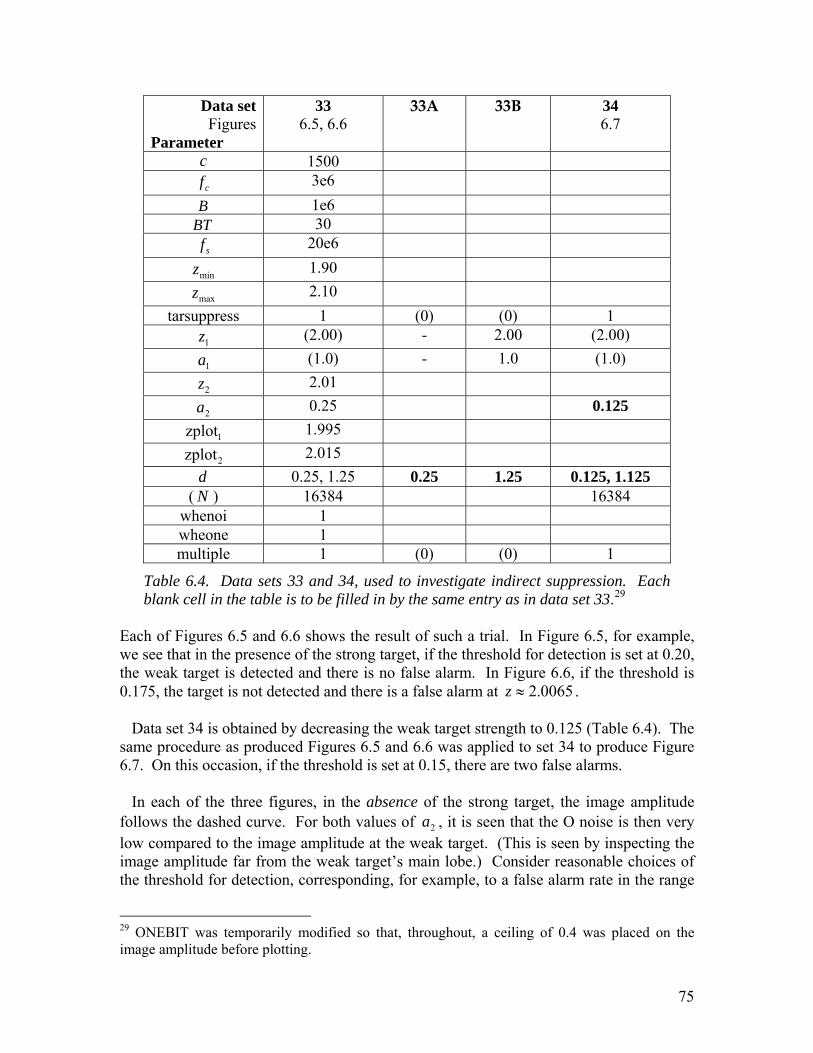
Data set Figures

Parameter

33 6.5, 6.6

33A 33B 34 6.7

c 1500 cf 3e6

B 1e6 BT 30

sf 20e6

minz 1.90

maxz 2.10 tarsuppress 1 (0) (0) 1

1z (2.00) - 2.00 (2.00)

1a (1.0) - 1.0 (1.0)

2z 2.01

2a 0.25 0.125

1zplot 1.995

2zplot 2.015 d 0.25, 1.25 0.25 1.25 0.125, 1.125

( ) N 16384 16384 whenoi 1 wheone 1 multiple 1 (0) (0) 1

Table 6.4. Data sets 33 and 34, used to investigate indirect suppression. Each blank cell in the table is to be filled in by the same entry as in data set 33.29

Each of Figures 6.5 and 6.6 shows the result of such a trial. In Figure 6.5, for example, we see that in the presence of the strong target, if the threshold for detection is set at 0.20, the weak target is detected and there is no false alarm. In Figure 6.6, if the threshold is 0.175, the target is not detected and there is a false alarm at 0065.2≈z . Data set 34 is obtained by decreasing the weak target strength to 0.125 (Table 6.4). The same procedure as produced Figures 6.5 and 6.6 was applied to set 34 to produce Figure 6.7. On this occasion, if the threshold is set at 0.15, there are two false alarms. In each of the three figures, in the absence of the strong target, the image amplitude follows the dashed curve. For both values of , it is seen that the O noise is then very low compared to the image amplitude at the weak target. (This is seen by inspecting the image amplitude far from the weak target’s main lobe.) Consider reasonable choices of the threshold for detection, corresponding, for example, to a false alarm rate in the range

2a

29 ONEBIT was temporarily modified so that, throughout, a ceiling of 0.4 was placed on the image amplitude before plotting.

75

0.1% to 10%. Considering that the noise amplitude distribution has an exponential tail, it is clear that in all cases the threshold is considerably less than the weak target’s peak amplitude. It follows that, in the absence of the strong target, the weak target is always detected (for the sets 33 and 34); the detection rate is 100% for all practical purposes. For the simulation, we need to decide on a false alarm rate. For an imaging sonar, it is appropriate to choose a considerably higher false alarm rate than for a sonar that seeks to detect, for example, a distant ship. A false alarm rate of 2% seems reasonable and so, for the simulations of this subsection, we choose that value. In the remainder of the sub-subsection we give an initial account of the remaining steps. The next step is to estimate the final, or 2%, threshold value of the image amplitude based on the 2% criterion. One approach to this is to estimate ( )rmsnp (a measure of the O-noise level) and use the distribution given by assumption 1 of the noise model to obtain the threshold. But there are at least two problems with this procedure. First, assumption 1 has not been tested. And second, the theoretical calculation must combine the O noise with the sidelobe amplitude due to both the strong and the weak targets. In view of the less-than-certain assumption (assumption 1) and the somewhat long chain of reasoning involved in the second point, this approach was rejected. Instead, it was decided to determine the 2% threshold value empirically, via simulations. The relevant threshold is the one that applies when the strong target is present. For each ‘present’ run, for each tentative threshold, the false alarms lying in the interval (6.11) are counted. We thus obtain a false alarm rate for each tentative threshold. Interpolation, to produce the 2% rate, yields the final threshold. The final step is to use the 2% threshold to determine the fraction of occasions on which the weak target is detected (in the presence of the strong target). Because these are detections of a true target, the fraction could be called the ‘true-detection rate.’ For convenience, the simple term detection rate will be used.30 It turns out that there is a very different detection rate for a target strength of 0.125 than for a target strength of 0.25. Actually the measured thresholds are affected by the presence of sidelobes of the weak and strong targets, and a correction must be calculated for this effect—at least in the weak-target case. Discussion of the corrections is postponed to Section 6.3.6. 6.3.3 Results of Simulation For data set 33, a series of 20 trials, each with its own noise stream, were performed, to generate pairs of image amplitude curves as exemplified in Figures 6.5 and 6.6. In each

30 This entails that henceforth a ‘detection’ means a detection of a true target. For the all-inclusive meaning of ‘detection’ we substitute a longer phrase, for example, an ‘apparent detection’ or a ‘detection or false alarm.’

76

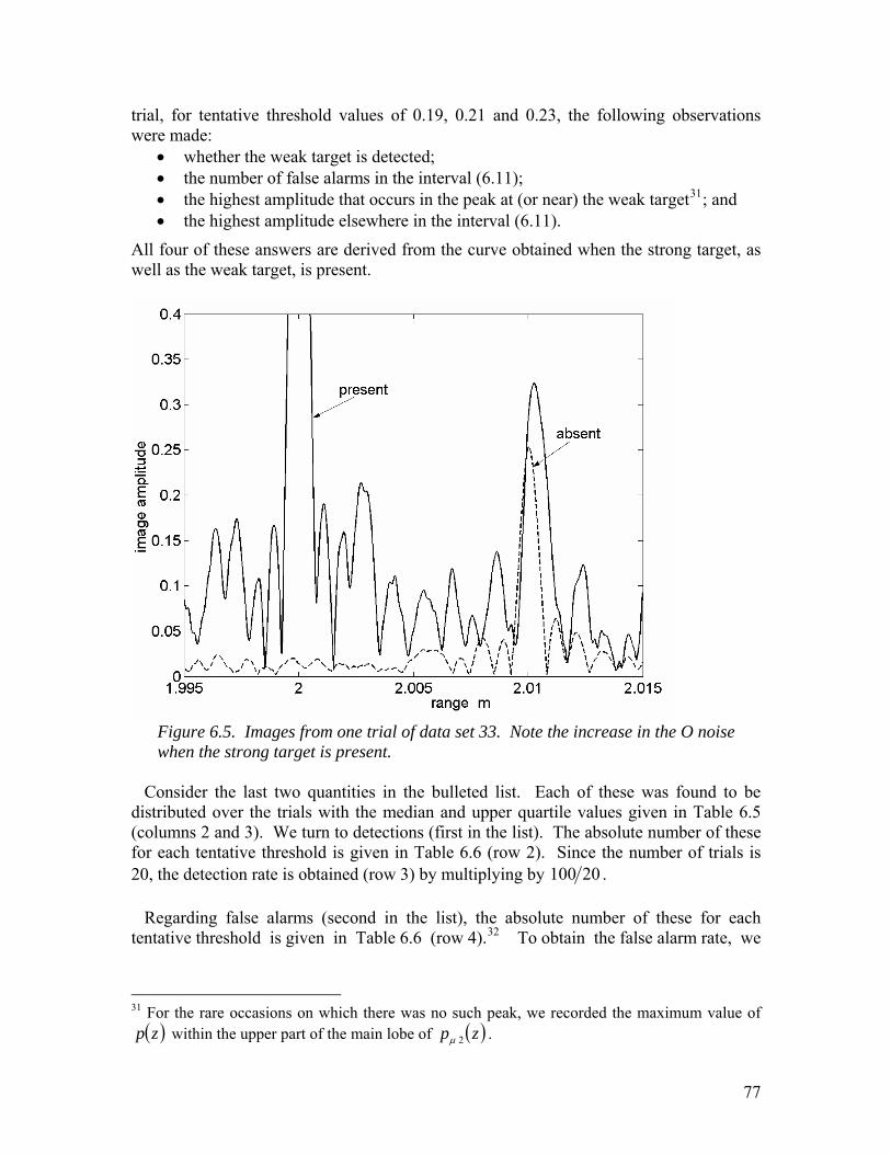
trial, for tentative threshold values of 0.19, 0.21 and 0.23, the following observations were made:

• whether the weak target is detected; • the number of false alarms in the interval (6.11); • the highest amplitude that occurs in the peak at (or near) the weak target31; and • the highest amplitude elsewhere in the interval (6.11).

All four of these answers are derived from the curve obtained when the strong target, as well as the weak target, is present.

Figure 6.5. Images from one trial of data set 33. Note the increase in the O noise when the strong target is present.

Consider the last two quantities in the bulleted list. Each of these was found to be distributed over the trials with the median and upper quartile values given in Table 6.5 (columns 2 and 3). We turn to detections (first in the list). The absolute number of these for each tentative threshold is given in Table 6.6 (row 2). Since the number of trials is 20, the detection rate is obtained (row 3) by multiplying by 20100 . Regarding false alarms (second in the list), the absolute number of these for each tentative threshold is given in Table 6.6 (row 4).32 To obtain the false alarm rate, we

31 For the rare occasions on which there was no such peak, we recorded the maximum value of

within the upper part of the main lobe of ( )zp ( )zp 2μ .

77

Figure 6.6. Images from another trial of data set 33.

25.02 =a (set 33) 125.02 =a (set 34)

Parameter At or near target

Away from target

At or near target

Away from target

median 0.251 0.1875 0.116 0.160 upper quartile 0.2885 0.210 0.141 0.177

Table 6.5. Consider the highest image amplitude obtained in the relevant region (picked out in the second row) in each trial. The distribution of these highest values has the median and upper quartile values shown. Number of trials is 20 for set 33, 40 for set 34.

Tentative threshold 0.19 0.21 0.23

Detections 17 14 12.5 Detection rate (%) 85 70 62.5 False alarms 11.5 4.5 0

Hypothesis Bc 4 Bc 2 Bc 4 Bc 2 Bc 4 Bc 2 False alarm rate (%) 2.3695 4.739 0.9272 1.8544 0.0 0.0

Table 6.6. Detections and false alarms for data set 33. Number of trials = 20.

32 It might be thought that, on occasion, it would be unclear whether a peak lying close to the weak target position should be counted as a (true) detection or a false alarm. In practice, no such difficulty was encountered.

78

must invoke the hypothesis, either (6.6) or (6.10), giving the length of the axis ‘occupied’ by one independent value of the complex O noise. On the

zBc 4 hypothesis,

this length is . The number of such lengths in the interval (6.11) is 26.667; on the

m 10375.0 3−×Bc 2 hypothesis, the number is half of this. However, these two results are slight

overestimates, because our procedure can never result in a false alarm close to the weak target: a high amplitude there is always interpreted as simply a detection. We now correct for this. By eye, it was judged that there is an interval of , centred on the weak target, of size about 0.90 mm, in which no false alarm can be recorded. On this basis, the number of potential occasions for a false alarm shrinks by a factor

z

( ) 01.00009.00100.0 − ; in place of 26.6667 the number becomes 24.2667 (but half of this on the Bc 2 hypothesis). In 20 trials the number of occasions is 20 times as great. This leads to the false alarm rates given in the last row of Table 6.6. For example, the first entry (2.3695) is calculated as ( ) ( )2026667.241005.11 ×× .

Figure 6.7. Images from a trial of data set 34. has been reduced to 0.125. 2a

Data set 34 was treated similarly. This time 40, rather than 20, trials were performed, to generate pairs of image amplitude curves as in Figure 6.7. The threshold values were changed slightly to 0.16, 0.18 and 0.20. As before, the distribution of the two highest amplitudes is found; the median and upper quartile values are shown in Table 6.5 (last two columns). The number of detections and false alarms, and the rates derived from them as before, are shown in Table 6.7. (An excluded interval of 0.90 mm is again used.)

79

Tentative threshold 0.16 0.18 0.20

Detections 5.5 2 1 Detection rate (%) 13.75 5.0 2.5 False alarms 27.5 8 1

Hypothesis Bc 4 Bc 2 Bc 4 Bc 2 Bc 4 Bc 2 False alarm rate (%) 2.833 5.667 0.824 1.648 0.103 0.206

Table 6.7. Detections and false alarms for data set 34. Number of trials = 40. 6.3.4 Analysis of Results The estimation of the 2% threshold will be illustrated by considering the case taken with the

25.01 =aBc 4 hypothesis. Perusal of the bottom line of Table 6.6 shows that, to

achieve 2%, we must interpolate between the tentative thresholds of 0.19 and 0.21. As the number of false alarms is expected to fall more or less exponentially with the tentative threshold, it is assumed that the false alarm rate is of the form ( )bxa −exp , where x is the (tentative) threshold. This gives a value 0.1936 for the 2% threshold, as given in Table 6.8. To estimate the detection rate at this threshold, it is assumed that the detection rate (row 3 of Table 6.6) also has an exponential dependence on the threshold between the threshold values 0.19 and 0.21. The resulting detection rate, to be called the raw detection rate, comes out to 82.1%, as given in Table 6.8. The same procedure is used to determine the raw detection rates in the other columns. 25.02 =a 125.02 =a Hypothesis Bc 4 Bc 2 Bc 4 Bc 2

2% Threshold 0.1936 0.2084 0.1656 0.1769 Raw detection rate (%) 82.1 71.1 10.3 5.8 Corrected detection rate (%) 81.7 70.5 8.5 3.9

Table 6.8. Thresholds and detection rates, based on a 2% false alarm rate. The raw detection rate overestimates how well the system performs at detecting the target. For suppose the raw detection rate were as low as the false alarm rate—2%, or more generally, . Then the system is detecting no more apparent targets than if there had been no target at all. Only the excess of the detection rate over counts as genuine detection performance. We therefore define a corrected detection rate, , for a given raw detection rate, , as follows. An

%l%l

%y%x x value of is to be mapped into a

value of zero, and an l y

x value of 100 is to be mapped into a value of 100. Requiring the mapping to be linear yields

y

( ) ( )llxy −−= 100100 (6.12)

80

Equation (6.12), with , yields corrected detection rates in the bottom row of Table 6.8.

2=l

6.3.5 Discussion Let us first discuss the results on the basis of the Bc 4 hypothesis. Table 6.8 shows that for the case 25.012 =aa , the introduction of the strong target produces a moderate drop in the corrected detection rate, from 100% to 82%. For the case 125.012 =aa , the drop in the corrected detection rate is severe, from 100% to a mere 8.5%. Somewhere in between there is a value of 12 aa at which the detection rate becomes 50%; this may be said to mark the borderline between a weak target that is suppressed by the indirect effect and one that is not. The borderline may be estimated by (i) first assuming that the corrected detection rate rises exponentially with 12 aa and thus estimating the borderline; then (ii) second, assuming a linear relationship (in place of the exponential one) and recalculating the borderline; and finally (iii) pooling the two answers, giving somewhat more weight to answer (i). The resulting borderline value of 12 aa is 0.210 to 0.218—on the Bc 4 hypothesis. The same calculation performed on the Bc 2 hypothesis yields a borderline value 0.223 to 0.230. Note that the borderline value is quite insensitive to whether the Bc 4 or the Bc 2 hypothesis is assumed, adding to the credibility of the result for the borderline value of 12 aa . These conclusions hold only for the case where there is no third target, or where any additional targets have strengths too small to have an appreciable effect on the minimum allowed value of the noise amplitude . d On the face of it, therefore, any second target with strength less than about 22% of the first target’s strength is not detected, due to the indirect effect. (The figure of 22% is in fact the best compromise between the Bc 4 and the Bc 2 hypothesis.) But this figure was obtained under very restricted conditions (e.g. a particular value of ). We now attempt to generalise the 22% result.

sf

First, let us consider whether changing the position of the target to be detected affects the detectability. We have already seen (Section 4.3.4) that the O noise is independent of . Hence, when is changed, the borderline value of

z

z z 12 aa should change rather little. (An exception occurs if is close enough to the strong target so that the strong sidelobe’s amplitude becomes an appreciable fraction of the rms O noise.) This claim will be confirmed in Section 6.3.6.

z

Regarding further generalisations, note that all the above results have been obtained with one particular set of values of , , cf sf B and T . In particular, the simulation used a rather low value of BT , namely 30.

81

Consider the effect of changing the chirp duration T . From Section 4.2, the O noise is proportional to T1 . As detectability is governed by the ratio of to O noise, the borderline value of

2a

12 aa should be proportional to T1 ; thus long chirps favour detectability. By arguments similar to those used in Section 4.2, we have the following results. The borderline value of 12 aa is proportional to sf1 , where is the sampling frequency. The borderline value is independent of both the central frequency and the bandwidth

sf

cfB .

We thus obtain, for a 50% probability of detection,

Tfaa

s

60022.0border1

2 ≈⎟⎟⎠

⎞⎜⎜⎝

⎛ (6.13)

subject to the low-sidelobe condition (6.1) (Table 6.4 has been used). Raising to make , reduces the borderline ratio from 22% to 3.8% (from Eqn 6.13), which seems satisfactory in an imaging system. This is not the end of the matter, however. When further strong targets are added into the field of view, the borderline ratio will rise again and may become unfortunately high. Still, it is to be noted that the findings to date are restricted to one dimension (the range); it is to be hoped that in three dimensions the situation regarding suppression is better.

T 1000=BT

Let us turn briefly to arrays that produce 3-D images. The O noise should depend very much on the number of elements. (By contrast, in the 1-D case, the number is only one). Hence the outcome in regard to suppression should likewise depend on this number. It is reasonable to expect that the suppression problem goes away when the number of elements is made large enough. Meanwhile, with regard to the 3-D system, we can only warn that indirect suppression is a potential problem, requiring further study. 6.3.6 Corrections for Sidelobes When sidelobes are present due to targets other than the one that is a candidate for detection, for a given tentative threshold, there is a rise in both the number of detections and the number of false alarms. We now estimate the effect of this on the numerical results calculated in Sections 6.3.3 to 6.3.5. We begin by studying the sidelobe effect due to the weak target; its effect turns out to be more important than that due to the strong target. 6.3.6.1 Sidelobes of Weak Target Clearly, when estimating the number of detections, the simulation should be performed with the weak target present—as was done. However, when estimating the number of false alarms (at a given tentative threshold), the simulation should be performed with the weak target absent—contrary to what was done in Section 6.3.3. Fortunately, with the aid of the image noise model, we can make corrections for the presence of the prior weak target. (The prior target is the one that was already known to be present; in that context,

82

a false alarm is an alleged detection of a second weak target.) Thus we can recalculate the quantities of interest in Sections 6.3.3 to 6.3.5. The calculation is done in Section G.1 of Appendix G. The results, after being corrected in this way, are given in Tables G.1 and G.2. The quantities calculated are not changed qualitatively by the correction. (The largest percentage change occurs in respect of the number of false alarms in the case where

and the middle tentative threshold (0.21) is used. Whereas 4.5 alarms were detected, there would have been only 3.33 alarms had the prior target been absent.) Furthermore, the next paragraph shows that the main result is hardly changed at all.

25.02 =a

The result of most importance concerns Equation (6.13) for the borderline value of

12 aa , set by a 50% probability of detection (the result is not in the two tables). The only change is that the 0.22 should be replaced by 0.215, so that Equation (6.13) is replaced by

Tfaa

s

600215.0border1

2 ≈⎟⎟⎠

⎞⎜⎜⎝

⎛ (6.14)

The difference is hardly significant; essentially the important result, Equation (6.13), is confirmed. Noting that is the number of points sampled during one chirp, we may rewrite Equation (6.14) as

TfN sT =

TNaa 27.5

border1

2 ≈⎟⎟⎠

⎞⎜⎜⎝

⎛ (6.15)

6.3.6.2 Sidelobes of Strong Target To recapitulate, we have calculated a number of properties (including the 2% threshold and the 50% borderline value of 12 aa ) and corrected them for the sidelobes of the weak target. In regard to the strong target, the first point to make is that these calculated properties are correct, when it is given that detections are being sought at points lying in a certain part of the strong target’s sidelobe pattern. (Under those conditions, no correction is needed and the heading of Section 6.3.6 is slightly misleading.)

z

To see this, note that, at a given , a sidelobe contribution to boosts the likelihood of a false alarm. Hence there is actually a different 2% threshold at each point , due to the dependence of the sidelobe strength on . What we would like to obtain is the threshold at the position of the weak target. Because the interval (6.11) is centred on the weak target, the threshold obtained (which is some average over the interval 6.11) should lie close to the desired value.

z apz

z

We wish to generalise. That is, we wish to state, for a general chirp system, at what scaled distance from the strong target the above calculated properties become appropriate. We do this by describing via a dimensionless parameter z ζ . Equations (3.5) and (3.9) show that the image amplitude, at each sidelobe peak, is given by

83

tBaa

pππζ

11peak s ≡= (6.16)

where and the s is for strong. ( 112 zzct −= − ) ζ is usually, to a good approximation, the

displacement 1zz − , measured in units of the distance from the main peak to the first null. Now at the centre of the interval (6.11) (which coincides with the weak target at

), the parameter has the value 01.2=z 33.13=ζ (from Table 6.4). Hence, as a first estimate, the property values obtained so far are particularly appropriate for possible detections around 33.13=ζ . An argument in Section G.2 indicates that a better statement is the following: it is in the interval 3.134.11 ≤≤ ζ that the property values obtained are most appropriate. We shall take the value 12.4 as typical of this interval. Some interest attaches to extending the results from 4.12=ζ to other values of ζ . There is particular interest in the Z region, 21 cTzz >− ; there the sidelobe amplitude is zero (from Eqn 3.5), but the rms O noise has the same value as at 4.12=ζ (from Section 4.3.4). In that region, indirect suppression continues to occur, the only difference being that the sidelobe amplitude, (s for strong), which was already small compared to sp p itself, is reduced to zero. We have not calculated in detail the effect, on the calculated properties, of moving from

4.12=ζ to the Z region. However, arguments given in Section G.2 lead to the following conclusion. It is considered more likely than not that the move produces a change in the borderline value of 12 aa that is no greater than 0.004 (which was the change due to removing the prior weak target). If the latter is true, the borderline value of 0.215 (Section 6.3.6.1) is changed to a value lying in the interval ( )22.0,21.0 . Furthermore, these statements clearly apply to a move from 4.12=ζ to any larger value of ζ (not necessarily lying beyond the sidelobes). 6.4 A Comment In retrospect, in this Section 6, the arguments depend very little on the assumptions of the image noise model. Consider first Section 6.1 (low sidelobe level). While the model was assumed when making numerical estimates within Section 6.1.1, the primary purpose there was to ensure that indeed the situation treated is low-sidelobe. The treatment of suppression itself, given in Section 6.1.2, makes no use of the model whatever. Now consider Section 6.2 (high sidelobe level). The model was assumed in Section 6.2.1, essentially to ensure that the situation treated is high-sidelobe. In regard to the tests for suppression, it is close to the truth to say that reliance is placed only on qualitative, not quantitative, features of the model.

84

In Section 6.3 (indirect suppression), no use was made of the model in the core calculation that extends to the end of Section 6.3.5. The model was used only in making the small corrections of Section 6.3.6.

7. Conclusions We shall pass over the many minor results obtained in this paper, and summarise the more important results. In Section 1 we showed by simulation how the process of adding noise prior to one-bit sampling effectively produces several-bit performance—provided that this process is combined with a subsequent operation of averaging over many samples. To avoid ghosts, it is highly desirable for the output signals, ( )twa and , to be linear in the input signal . Section 4 showed that for the system that combines added noise, one-bit sampling and cross-correlation, the output signals are linear in the mean, provided that the noise voltage has a uniform distribution and the noise amplitude exceeds the maximum value of

( )zpa

( )tu

d( )tu (Eqn 4.3). In the context where one requires strict

linearity in the mean, Equation (4.3), but construed as an equality, gives the optimum value of . With this value of , full linearity is approached as the chirp duration T approaches infinity, since the image noise approaches zero.

d d

When there are more than a couple of targets, it is no longer appropriate to require strict linearity in the mean. The optimum value of is then lowered below the value given by (4.3). The reason is that a small degree of ghosting is accepted in exchange for the ability to detect more targets.

d

As stated earlier, some key parts of these ‘linearity’ results were known to workers, such as D.E. Robinson and Ian G. Jones, involved in the underwater acoustic imaging project mentioned above; however it seems that none of these particular results have been stated previously in the literature. In Section 4, a model for the image noise was proposed. Most of its assumptions were tested and corroborated. It was shown that the rms image noise 1τ is given, under very general conditions, by Equation (4.22), namely

TNd78.11 ≈τ (7.1) where is the number of points sampled during one chirp. This result applies to the one-element case. For an array of many elements, used to produce a 3-D image, two things can be said. First, the result (7.1) continues to apply to the output of each element. Secondly, one would expect that the value of the image noise, relative to the image ‘signal,’ is lower, and hence better, than what Equation (7.1) predicts.

TfN sT =

( )tw

85

Section 5 took up a suggestion that had worked well in a one-bit but non-imaging context. This is the idea that, following one-bit digitisation, filtering should produce a marked improvement towards ‘recovering’ the output signal that would have been obtained had E sampling been used. Contrary to the suggestion, it was found that: (i) filtering is unnecessary, as the cross-correlation already does quite a good job of filtering out components lying outside the band of width B , and (ii) the added filtering makes the image worse. The reason for these results is believed to be that the cross-correlation provides the optimal filtering for recovering the desired signal. In Section 6 on suppression of a weaker target, the main interest is in the case of indirect suppression, where the strong target pushes up the optimal value of . In the course of this investigation, we estimated the number of independent values of the image amplitude per unit interval of , essentially narrowing the answer down to two possibilities. For the case where there are just two targets (the strong and the

d

z

weak), we estimated the borderline value of the ratio 12 aa , defined as the value such that the weak target has a probability of 50% of being detected. Our conclusion is that, under very general conditions, the borderline value of 12 aa is given by Equation (6.15), namely

TNaa 27.5

border1

2 ≈⎟⎟⎠

⎞⎜⎜⎝

⎛

This result applies to the one-element case; one would expect the right-hand side to be replaced by a lower value when many elements are processed to form a 3-D image.

Acknowledgments This paper has benefited from discussions with David Robinson, Phil Ho and Donald McLean of CSIRO (Commonwealth Scientific and Industrial Research Organisation) Division of Telecommunications and Industrial Physics (TIP) and Ian G. Jones of Thales Underwater Systems.

References Aziz, P. M., Sorensen, H. V. and van der Spiegel, J. (1996). An Overview of Sigma-Delta Converters. IEEE Signal Processing Mag., Jan. 1996, pp. 61–84.

Bateman, A. and Yates, W. (1988). Digital Signal Processing Design. London: Pitman.

Bellanger, M. (1984). Digital Processing of Signals. New York: John Wiley.

Bennet, W. R. (1948). Bell Syst. Tech. J., 27, p. 446.

Benzi, R., Sutera, A. and Vulpiani, A. (1981). J. Phys. A, 14, L453.

Bergland, G. D. (1969). A Guided Tour of the Fast Fourier Transform. IEEE Spectrum, 6, pp.41–52.

86

Bingham, C., Godfrey, M. D. and Tukey, J. W. (1967). “Modern Techniques of Power Spectrum Estimation,” IEEE Trans. Audio and Electroacoustics, AU-15, pp. 56–66, June 1967.

Blair, D. G. and Anstee, S. D. (2000). Underwater Acoustic Imaging: A Simulation Program and Related Theory. (DSTO Technical Note DSTO-TN-0274). Melbourne: Aeronautical and Maritime Research Laboratory.

Bulsara, A. R. and Gammaitoni, L. (1996). Tuning in to Noise. Physics Today, March 1996, pp. 39–45.

Burdic, W. S. (1991). Underwater Acoustic System Analysis, 2nd Ed. Englewood Cliffs, New Jersey: Prentice-Hall.

Ditchburn, R. W. (1952). Light. London: Blackie.

Freeman, S. R., Quick, M. K., Morin, M. A., Anderson, R. C., Desilets, C. S., Linnenbrink, T. E. and O’Donnell, M. (1997). Ultrasound Beamformer using Oversampling. In: Proceedings of the IEEE Ultrasonics Symposium, Vol. 2, pp. 1687–1690 (conference held at Toronto, Canada, 5–8 Oct. 1997). New York: IEEE Press.

Freeman, S. R., Quick, M. K., Morin, M. A., Anderson, R. C., Desilets, C. S., Linnenbrink, T. E. and O’Donnell, M. (1999). Delta-Sigma Oversampled Ultrasound Beamformer with Dynamic Delays. IEEE Trans.on Ultrasonics, Ferroelectrics, and Freq. Control, 46, pp. 320–332.

Gammaitoni, L. (1995). Stochastic Resonance and the Dithering Effect in Threshold Physical Systems. Phys. Rev. E, 52, pp. 4691–4699.

Gammaitoni, L., Hanggi, P., Jung, P. and Marchesoni, F. (1998). Stochastic Resonance. Rev. Mod. Phys., 70, pp. 223–287.

Gingl, Z., Vajtai, R. and Kiss, L. B. (2000). Signal-to-Noise Ratio Gain by Stochastic Resonance in a Bistable System. Chaos, Solitons and Fractals, 11, pp. 1929–1932.

Han, H.-S., Park, H.-J. and Song, T.-K. (2002). A New Architecture for Ultrasound Sigma-Delta Modulation Beamformer. In: Proceedings of the IEEE Ultrasonics Symposium, 2002, Vol. 2, pp. 1631–1634 (conference held at Munich, Germany, 8–11 Oct., 2002). New York: IEEE Press.

Hogbom, J.A. (1974). Aperture Synthesis with a Non-Regular Distribution of Interferometer Baselines. Astronomy and Astrophysics, Supplement Series, 15, no.3, pp. 417–426.

Jones, I. S. F. (1996). Underwater Acoustic Imaging Innovation Program (DSTO Technical Note DSTO-TN-0065). Melbourne: Aeronautical and Maritime Research Laboratory.

Kino, G. S. (1987). Acoustic Waves: Devices, Imaging, and Analog Signal Processing. Englewood Cliffs, New Jersey: Prentice-Hall.

Kozak, M. and Karaman, M. (2001). Digital Phased Array Beamforming Using Single-Bit Delta-Sigma Conversion with Non-Uniform Oversampling. IEEE Trans. On Ultrasonics, Ferroelectrics, and Freq. Control, 48, pp. 922–931.

87

Maguer, A., Vesetas, R. and Azemard, F. (2000). 3D Acoustic Imaging of Objects in Water. Acoustics 2000: Proceedings of Australian Acoustical Society Annual Conference, held at Joondalup Resort, Western Australia, 15–17 Nov. 2000, pp. 87–93. Perth, W.A.: Australian Acoustical Society.

Manzie, G. (2000). High Resolution Acoustic Mine Imaging. UDT Pacific 2000: Undersea Defence Technology, Darling Harbour, N.S.W., Australia, 7–9 February, 2000, pp. 356–359. Swanley, Kent, U.K.: Nexus Information Technology.

McNamara, B., Wiesenfeld, K. and Roy, R. (1988). Phys. Rev. Lett., 60, 2626.

Moss, F. and Wiesenfeld, K. (1995). The Benefits of Background Noise. Scientific American, Aug. 1995, pp. 50–53.

Rihaczek, A. W. (1985). Principles of High-Resolution Radar, Revised Version. Los Altos, Calif.: Peninsula.

Spiegel, M.R. (1968). Mathematical Handbook of Formulas and Tables. New York: McGraw-Hill (Schaum’s Outline Series).

Steinberg, B. D. (1976). Principles of Aperture and Array System Design—Including Random and Adaptive Arrays. New York: John Wiley.

Steinberg, B. D. (1984). Adaptive Beamforming of Distorted Microwave Imaging Antenna Arrays Using Radiation-Field Measurements. Proceedings of the 27th Midwest Symposium on Circuits and Systems, Vol. 2, pp. 550–553. Pub. by West Virginia University.

Steinberg, B. D. and Subbaram, H.M. (1991). Microwave Imaging Techniques. New York: John Wiley.

Tukey, J. W. (1967). “An Introduction to the Calculations of Numerical Spectrum Analysis.” In: Harris, B. (ed.), Spectral Analysis of Time Series, pp. 25–46. New York: Wiley.

Van Vleck, J. H. and Middleton, D. (1966). The Spectrum of Clipped Noise. Proc. of IEEE, 54, pp. 2–19.

Vesetas, R. and Manzie, G. (2001). AMI: A 3-D Imaging Sonar for Mine Identification in Turbid Waters. Oceans, 2001: MTS: IEEE Conference and Exhibition, Honolulu, 5–8 Nov. 2001, Vol. 1, pp. 12–21. New York: IEEE Press.

Weinreb, S. (1963). A Digital Spectral Analysis Technique and its Application to Radio Astronomy (Technical Report 412). Cambridge, Mass.: Research Laboratory of Electronics, Mass. Institute of Technology.

Ziomek, L. J. (1985). Underwater Acoustics: A Linear Systems Theory Approach. New York: Academic Press.

88

Appendix A: Shift of jw Shifts arise from two sources. The first shift occurs because the received signal (associated with ) begins at some time after the time at which the signal starts being transmitted. The second shift arises from the dechirping (cross-correlation) operation.

v s

In regard to the first shift, the user specifies and , the minimum and maximum ranges at which targets may occur. The program then calculates the time

minz maxz

czz

f s

minmax +=′δ

at which the reflection from a target at the centre of the allowed interval of ranges would return to the receiver. Let δ be δ ′ but rounded to the nearest integer. The centre, in time, of all the samples of the return signal is taken to be at sft δ= . As the centre of the transmitted signal is at , there is a time-shift of 0=t δ samples between the centre of the samples and the centre of the samples . js jv Table A.1 shows where the various signals are centred, both as a function of j and as a function of time. Always the index j of a vector runs through the values . ‘Centred’ at P means that the absolute value of the vector or signal would be symmetric about P if the targets were distributed symmetrically about

Nj ...,,2,1=

( ) 2minmax zzz += . In the last row of the table, Equation (2.24) has been used. It follows that the remaining time-index relationships are

( ) ( )( ) NNjfNj

Njfjt

s

sj

...,,12 12...,,1 1

+=+−−=

=+−=

δ

δw (A.1)

Vector Value of j at centre Value of t at centre

s ( )121 +N 0

u , q ( )21

21 within 1 ±+N sfδ ′

w

21thin wi1 ± sfδ ′

ew 21

21 within 1 ±+N sfδ ′

Table A.1. Showing where the various signals (vectors) are centred. The row for and q applies also to and . Each row applies not only to the in-phase

signal but also to the corresponding analytic signal. u u′ v

89

for the vector , and Equation (2.25) for . Note that in the case of , because the distribution is centred on the end element

w ew w1=j (Table A.1), wrap-around plays an

essential role (Equation A.1). For this reason it is preferable to work with the vector rather than when, for example, one is displaying a graph of the vector (i.e. element versus index).

eww

Appendix B: Filtering B.1 General The filter function defined in the main text has the form ( )fH 0

( ) ( )

( ) 2 0

22

2sin1

2 1

21

0

AEf

AEfAEEfA

AEffH

+≥=

+<<

−

⎭⎬⎫

⎩⎨⎧

⎥⎦

⎤⎢⎣

⎡⎟⎠⎞

⎜⎝⎛ −−=

−≤=

π (B.1)

( )fH 0 may be written as

( ) ( ) ( ) ( ) ( ) ( ) ( ) fdfGffJAfGfJAfH ′′′−=∗= ∫220 ππ (B.2) where ∗ is the continuous, non-wrapped convolution operation and

( ) ( )EffJ rect= (B.3) ( ) ( )

2 0

2 cos

Af

AfAffG

≥=

<= π (B.4)

(Fig. 2.2b). The inverse Fourier transforms are ( ) ( ) ( ) ( )tgtjAth 20 π= (B.5)

( ) ( ) ( ) EtEtEEtEtj ππsinsinc == (B.6)

( ) ( )( )

412

cos2 −

−=At

AtAtg ππ

(B.7)

The total power (i.e. time-power) of ( )th0 is

( ) ( ) ( AEdffHdtthV −==≡ ∫∫∞

∞−

∞

∞−

4412

0

2

0 ) (B.8)

the calculation being performed in frequency domain. The power beyond is t±

( ) ( )[ ] ( )[ ] dssgsjAWt

22222 ∫∞

= π

By replacing the sine in (B.6) by unity, we have ( )[ ] 222 1 ssj π≤ (B.9)

From (B.7) we also have

90

( )[ ] ( ) ( ) ( )2

412422 2

−

⎥⎦⎤

⎢⎣⎡ −≤ AtstAsg π (B.10)

Hence we obtain a bound on W , so that the fraction ( ) VWt =1θ of the power that lies beyond satisfies t±

( ) ( )[ ] ( ) ( )[ ] 225121 211410

−−−−−−≡≤ AtAtmUt πθ (B.11)

where AEm = . Let us relate to t K of the main text by tfK s2= ; then we have ( ) ( )tK 1θθ = . Suppose we wish to ensure that the power aliased satisfies (2.29), and let us choose

as in the main text. Then from (B.11) a sufficient condition comes out to be 21=m51.1≥At (B.12)

that is, AfK s02.3≥ . Let us choose 20BA = as in the main text; the result (2.30) follows. B.2 Dependence of Power Aliased on E (Qualitative) The following general remarks can be seen to apply by considering the various formulae in Appendix B.1. Suppose that each vector in time domain has elements and therefore occupies a total time

NsfN=τ . First, when E is sufficiently large (in

practice, very large) compared to τ1 , the fraction of the power aliased is very small, even with , that is, even without invoking a smoothing step in Figure 2.2(a). The smoothing step in the filter function is not needed.

0=A

Second, as E is reduced, next there is an interval of E such that, with , the power aliased is no longer very small, but can be made so by invoking a smoothing step of some sensible size

0=A

A . Third, when E is reduced further still, no value of A can keep the fraction of power aliased to the desired very small value. This is because, as E is reduced, the required value of A is forced up until it reaches say 3E (where the filter no longer approximates a rectangle) and eventually reaches the value E , the largest sensible value that A can have. B.3 Varying E and A Let be the right-hand side of Equation (B.11); it is the upper bound on the fraction of the power aliased (given that

( tAEUU ,,= )tfK s2= elements are set aside for nonzero

elements). The changes referred to in the main text take place at fixed . If we begin from the guessed optimum combination

t( )00 , AE —or any other sensible combination of

E and A — it can be shown from (B.11) that ( )tAEU ,, is reduced when any one of the following operations is carried out.

1. E is increased at fixed .A

91

2. A is increased at fixed AE − . 3. A is increased at fixed E .

(A first ‘cut’ at the proof is obtained as follows. To a first approximation, the term 1− in the first square bracket and the negative term in the second square bracket can be dropped. Then U is proportional to 41 −− AE ; and the results for operations 1 to 3 follow easily. A final ‘cut’ can be written down, in which the term –1 is retained.) Let us recall that the combination ( )00 , AE satisfies Equation (2.29). Starting from

, if an operation of type 1 to 3 is performed, (2.29) will still be satisfied, for U will have decreased. If, from the new starting point, another operation of type 1 to 3 is performed, because of the phrase ‘or any other sensible combination of

( 00 , AE )

E and A ,’ Equation (2.29) will again be satisfied. Similarly, given any combination that can be obtained from by a sequence of operations of the types 1 to 3, the aliasing continues to satisfy the criterion (2.29).

( AE, ))( 00 , AE

Appendix C: Ghosts in the Range Domain As a preliminary, consider the case of exact sampling, uv = . When there is just one target, located at , from (2.1) and (2.4), we have (apart from a constant of proportionality)

0zz =

( ) ( ) ( )[ ]{ }( )[{ 2

01

2000

2cos

5.02cos

bttbezfk

eztbeztfktv

c

c

+−+=

−+−+=

π

π

] } (C.1)

Here ce 2= , and , , etc. denote constants (independent of t ). (Here and in the rest of Appendix C, we ignore the fact that the chirp is of finite extent and, for simplicity, we ignore the quadrature terms.) As shown in Section 2, when is subsequently cross-correlated with to produce , and then evaluated at

0k 1k

vs w ezt = to produce the image ( )zp ,

a spike at is produced. It follows that, whenever 0zz = ( )tv contains a term of the form of the second line of (C.1), but with now given by some other expression independent of t , the image has a spike at (the new value of)

0z

0z . To focus on the essentials, we consider two targets, both of strength unity, located at and . Then

1z

2z( )[ ] ( )[ ]21 coscos ezteztu −+−= φφ (C.2)

where ( ) ( )2

3 5.02 bttfkt c ++= πφ The sum of cosines can be written as a product, and the cosines in the latter can be rewritten as sines, subject only to a change in the values of the relevant . The result is ik

( ){ } ( )[ ]{ }2215124 2sinsin2 bttzzbefktzzbeku c ++−+−+= ππ (C.3)

92

From the definition (2.11) of in one-bit, a little thought shows that (apart from a constant of proportionality) is given by the right-hand side of (C.3), but with sin replaced throughout by Sin, defined by

vv

0sin 10sin 1Sin

<−=>+=

xxx

Now versus xSin x is a square wave, and it is given (Spiegel, 1968, p. 132) by the Fourier series

( )xjj

xj

12sin12

14Sin 0

++

= ∑∞

=π

We now substitute this expression for both occurrences of Sin in , obtaining v

( ) ( ){ }

( ) ( )[ ]{ }2215

1240 0

2

212sin

12sin12

112

142

bttzzbefkl

tzzbekjlj

v

c

j l

++−++

×−++++

⎟⎠⎞

⎜⎝⎛= ∑∑

∞

=

∞

=

π

ππ (C.4)

We now ignore the terms . (These may lead to further distortion of the image, depending on whether these terms are filtered out in the operation .) The product of sines can then be converted back into a sum, yielding

0≠lwv →

(∑∞

=

−+

⎟⎠⎞

⎜⎝⎛=

0

2

coscos12

14j

FEj

vπ

) (C.5)

where ( ) ( ) ( )[ ]{ }( ) ( ) ( )[ ]{ }2

12217

212216

122

122

bttzzbejzzbefkF

bttzzbejzzbefkE

c

c

+−+++−+=

+−+−+−+=

π

π (C.6)

Comparing (C.5) and (C.6) with the last line of (C.1), we see that spikes occur at ( ) ( ) 22 1221 zzmzzz −++=

where (which may be positive or negative) is odd. The result is thus proved. m

Appendix D: Tail of Analytic Signal For data set 1, on the ‘outer’ side, tends to zero asymptotically in proportion to

, as a computation at selected points, using ONEBIT, shows.

is( ) 1

0−− tt

However, the simple proportionality to ( ) 1

0−− tt does not hold generally. A second run

was carried out with a shorter chirp ( BT equal to 30 instead of 300) and with reduced from 20 MHz to 10 MHz (data set 2 in Table 3.1). Note that this lower sampling frequency is close to the limit allowed by the Nyquist relation for this shorter chirp (the limit being at least 7.1 MHz and possibly as high as 8 MHz).

sf

93

To investigate the suggested proportionality, the product of 0tt − (or equivalently, ) and was plotted against time (Figure D.1). Naively this should be a constant,

beyond a few cycles from the chirp end. 0jj − i

js

It turns out that there is departure from constancy in two respects. First, the product oscillates. However, the oscillations become small, in relative terms, as the time moves further away from the chirp end. These oscillations are probably due to the close approach to the Nyquist condition. The frequency of the oscillations is 5.0 MHz. While we do not have a detailed explanation for this oscillation, the facts (i) that this frequency is not or cf 2Bfc ± , and (ii) that this frequency, 5.0 MHz, is just half of , strongly suggest that the oscillation is linked to the sampling frequency.

sf

The second departure concerns the local mean of the oscillatory pattern. As t increases, the local mean is roughly constant for a few cycles, but thereafter it steadily increases. We put forward the hypothesis that the latter increase is due to a similar

Figure D.1. Test of the ( relationship for the quadrature part of the chirp, for data set 2. The quantity plotted is multiplied by

) 10

−− tt isijs 0jj − , where j is

the index of the vector. and refer to the chirp end. The naïve prediction is that the product is a constant when ‘number of cycles’ (quantity along

0t 0jx axis) is

considerably greater than one.

94

( contribution produced by the other end of the chirp, with the same constant of

proportionality. Consider the ratio of the values of

) 10

−− tt1

0−− tt from the two ends (far end

divided by near end): this ratio becomes 0.31 at the right-hand end of the graph. If there are two contributions as stated, this value (0.31) should be the same as

( )[ ] MM−end hand-rightat mean local where M is the local mean value at its turning point near the chirp end. In fact the two are roughly equal (14% difference). The results are therefore consistent with the proposition that the two ends each produce a ( ) 1

0−− tt contribution.

Note that this appendix has been concerned only with matters of detail; the results stated in the main text regarding the behaviour on the ‘outer’ side are not in question.

Appendix E: Measures of Similarity We can describe the difference between the two image amplitude functions quantitatively as either the ‘power moved’ or ‘total amplitude moved,’ as follows. Consider first the ‘power moved.’ For generality, consider any two vectors and (where the index is essentially time or displacement). The first step is to multiply by

a constant so that the two total ‘powers’

1g 2g

2g2

∑ j ijg are equal. (Here, for each of 2,1=i ,

is the ijg j th element of .) (Here we speak of ‘power,’ even though we are dealing with a ‘spectrum’ in the time domain.) Then the measure

ig

∑ −=j jj gg

2

1

2

221PM (E.1)

is the power moved (in the sense that if pieces of power are moved from one value of j to another, this is the minimum amount of power moved that can accomplish the transformation from to ). The quantity 1g 2g

2

1PM ∑ j jg (E.2)

which is the fraction of power moved, is a measure of the overall discrepancy between and (the absolute scale of the vectors being ignored, only the shapes being retained). The alternative measure, using ‘total amplitude’ in place of ‘power,’ is described exactly as above but with all the squaring operations removed; in place of PM we write TAM.

1g

2g

Let us now apply these measures of difference to the error introduced by the continuous-time approximation (Section 3.3). Then and are the two image amplitude vectors shown in Figures 3.4 and 3.5. The fractional or percentage measures just defined come out to be 0.28% (in the case of power) and 1.29% (case of total amplitude). In this calculation, the full length of the vectors has been used, not just the portion that was plotted.

1g 2g

95

Actually the calculation just described does not give a check on the carrier-wave factor in Equation (3.5). A further test was therefore carried out as before, but with and , respectively, put equal to (i) the real part of the complex image amplitude, and (ii) the prediction that (3.5) gives. The respective percentage measures then come out to be 0.40% and 2.11%. Again, for the imaginary part, the respective percentage errors are 0.36% and 2.54%. We conclude that Equation (3.5) is good also in respect of the carrier wave.

1g 2g

Appendix F: Sidelobe and O-Noise Levels F.1 Low-Sidelobe Case We estimate the sidelobe and O-noise levels, for the purpose of checking that the low-sidelobe condition (6.1) is satisfied. The O-noise level is estimated approximately by examining the values with the strong target absent (assumption 4 of the image noise model used). In particular, the

( )zp( )zp values are examined for not near the weak target

(specifically, to 2.005) (assumption 2 used). The arithmetic mean of the z

995.1=z( ) ( )zpzp a= values over this interval is found by eye from the monitor display.33

(Strictly speaking, at each , z ( ) ( )zpzp ann = differs from this, due to the presence of the

term . However, when the correction required to obtain ( )zp a2μ ( )zpn was calculated it

was found to be negligible.) This arithmetic mean is averaged in turn over 7 trials, to yield the value . From assumptions 1 and 2 of the image noise model, for each the values should follow a probability density function of the form

( ) 1106.0meann =pz ( )zpn

( ) 0 ,exp 2 >− xbxax , where and b are independent of . Therefore the rms value should be

a zπ2 times the mean. Thus

( ) ( ) 1248.01106.02rmsn == πp (F.1) Next we estimate and hence ( )11 zpμ ( )21 zpμ . The former (which theoretically should be , from Eqns 3.5 to 3.8, and hence equal to unity from Table 6.1) is estimated by measuring the peak value (over ) of

1az ( )zp with the strong target present. The root-

mean-square value of the peak is taken over 7 trials, to yield ( ) 980.01rms =zp (F.2)

where the notation conforms to the definition to be given below Equation (F.3). rmsp

33 The mean is found by selecting the horizontal line such that the area below the p curve but above the line equals the area above the p curve but below the line.

96

This figure includes a contribution from O noise, for which a correction is to be made, evaluated as follows. Equation (4.17) can be rewritten as

an

aa ppp += μ where the argument has been dropped. We multiply each side of the equation by its complex conjugate and then take the expectation value over the noise stream. The two cross terms vanish since

z

0an =p . Hence

2an

2a2a ppp += μ

In turn this can be written as ( )2rmsn

22 ppp += μ (F.3)

where we write aμμ pp = . The left-hand side of (F.3) we also write, by definition, as

. Substituting (F.1) and (F.2) into (F.3), we obtain2rmsp 34

( ) ( ) ( ) ( )1a

122

11 972.01248.0980.0 zpzp μμ ==−= (F.4)

(Trivially, the last equality follows because, in Eqns 3.5 and 3.8, has the same phase as .)

( )1a

1 zpμ

1a Next, the value of relative to ( )2

a1 zpμ ( )1

a1 zpμ is calculated from the continuous-time

equations, (3.5) to (3.8). The result is combined with (F.4) to yield ( ) 0222.02

a1 −=zpμ (F.5)

In Section 3.3.1, we derived the conditions for constructive and destructive interference to occur at the weak target. In the present case, we have , 801 =m 72 =m ( π40.7phase = ) and , so that the interference is destructive, confirming the sign in Equation (F.5). From (F.1) and (F.5), the ‘low-sidelobe’ condition (6.1) is satisfied, the ratio of the two sides being 5.6.

03 =m

For completeness, is estimated as ( )2

a2 zpμ 12 aa times ( )1

a1 zpμ ; the result is

( ) 2430.02a

2 +=zpμ F.2 High-Sidelobe Case As stated in Section 6.2.1, we place the weak target at the peak of the strong target’s first sidelobe. Then, in Section 3.3.1, 91 =m is an integer. We assume that, since is unchanged from the weak-sidelobe case, from Equation (F.4) we still have

1a

34 An alternative method is simply to put ( )11 zpμ equal to (the theoretical value noted above). That method has the advantage that statistical fluctuations are removed. We have stayed with the method originally used, of which it can be said, at least, that it relies less heavily on the continuous-time approximation.

1a

97

( ) 972.01a

1 =zpμ (F.6) At the first sidelobe we therefore have

( ) ( ) 2063.0972.0322a

1 +=×+= πμ zp (F.7) from Equation (3.5). (The sign is positive since 101921 =+=+ mm is even.) To achieve the desired ratio (say 5) in (6.2), the O noise must be reduced from the value 0.1248 (Eqn F.1) used in the low-sidelobe case. We do this by increasing the pulse duration and invoking the T T1 proportionality in assumption 3 of the image noise model. Specifically, we raise BT from 30 to 300; this finally produces data set 32. We now have

( ) 03947.0101248.0rmsn ==p (F.8) From (F.7) and (F.8), the ratio of the two sides in (6.2) is 5.2; so the ‘high-sidelobe’ condition (6.2) is satisfied.

Appendix G. Correction for Sidelobes G.1 Sidelobes of Weak Target We calculate the effect of the prior weak target, ignoring the effect of the strong target. We may write , where the subscript w means ‘due to the (prior) weak target.’ For a given value of , from assumption 1 of the image noise model, the probability distribution of is a joint normal distribution, but with its centre shifted from the origin of the complex plane to the position (taken to be real and positive, without loss of generality). Let

aw

an

a ppp +=awps ≡

apsp =a

21τσ = . The probability density function of app = can be written down as an integral, which, when evaluated (Spiegel, 1968, p. 143), comes out to be

( ) ( ) ⎟⎠⎞

⎜⎝⎛

⎥⎦⎤

⎢⎣⎡ +−= 20

2222 2

1expPrσσσspIsppp (G.1)

where is a modified Bessel function. Next we wish to calculate , the probability of obtaining a ‘ ’ value greater than (a cumulative probability).

0I ( p>Pr )p p ( )p>Pr

is expressed as an integral over (say) p′ from to infinity. Our interest is in the case in which and is in the tail of the distribution. Then it can be shown that a good approximation is to put

pps << p

( ) ( )20

20 σσ spIpsI =′ . We thus obtain

( ) ( ) ( ) ⎟⎠⎞

⎜⎝⎛

⎥⎦⎤

⎢⎣⎡ +−=>≡ 20

2222

1expPrσσspIspppQ (G.2)

Thus, for a given , is enhanced, over the value it would have in the absence of the prior target, by

s ( )pQ

98

( ) ( )( ) ⎟⎟

⎠

⎞⎜⎜⎝

⎛−⎟

⎠⎞

⎜⎝⎛=≡ 2

2

200 2

expσσsspI

pQpQpR (G.3)

where and ( ) ( )[ ] 000 == spQpQ ( ) 100 =I . In the calculation of the enhancement factor, a complication arises because varies as

traverses the relevant region (which is s

z 015.2005.2 << z , but excluding the upper part of the main weak lobe). For this reason, in place of R we use a weighted value

∑ ∑=i iii wRwR

i, where i refers to the th point in the region. Let i φ be the argument

of the sine in the continuous-time approximation (3.5). The points selected are those for which

5...,,5.2,2,5.1,1=πφ The sequence is cut off at 5, because 5.5=πφ corresponds to a point beyond . The weight given to each of the two end-points (

015.2=z5 and 1=πφ ) is 0.5; the weight of all

other points is one. In calculating R via Equation (G.3), σ is obtained from the formula (4.22); is obtained from (3.5) and (3.9). The values of the tentative threshold

iss =p are the six values

used in Tables 6.6 and 6.7. Actually, the calculation was performed for only four of these. For , the values 0.19 (lower threshold) and 0.21 (middle threshold) (Table 6.6) were used; for , the values 0.16 (lower) and 0.18 (middle) (Table 6.7) were used. The results are given in Table G.1 (the

25.02 =a125.02 =a

R row). These factors R are applied to the data from Tables 6.6 and 6.7 to recalculate the number of false alarms and the false alarm rate (rows below the R row). In the table, the figure of 9.20, for example, is the estimated number of false alarms that would have occurred, had the prior target been absent.

2a 0.25 0.125 Tentative threshold 0.19

0.21 0.16 0.18

R 1.25 (1)

1.35 (1)

1.062 (1)

1.086 (1)

Number of false alarms 9.20 (11.5)

3.33 (4.5)

25.89 (27.5)

7.37 (8)

False alarm rate (%) 3.79 (4.739)

1.37 (1.854)

5.34 (5.667)

1.52 (1.648)

Table G.1. Values of false alarm rate and related quantities, after correction. Uncorrected values are given in parentheses. False alarm rates are based on the

Bc 2 hypothesis.

99

2a 0.25 0.125

2% threshold 0.2026 (0.2084)

0.1756 (0.1769)

Raw detection rate (%) 75.2 (71.1)

6.25 (5.8)

Corrected detection rate (%) 74.7 (70.5)

4.3 (3.9)

Table G.2. Values of detection rates and related quantities after correction. Otherwise as for Table G.1. Note that the figures 74.7 and 4.3 in the bottom cells have been doubly corrected.

Based on the corrected figures in the bottom row of cells of Table G.1, the 2% threshold is calculated as before (Table G.2). Using the new 2% threshold, the raw and corrected detection rates are also calculated as before (Table G.2).35

From the corrected detection rates (bottom row of cells), the 50% borderline value of

12 aa is estimated as before. Using exponential and linear interpolation and pooling the results, it is found that the borderline value is reduced by 0.004—on the Bc 2 hypothesis. On the Bc 4 hypothesis, the corresponding effect is expected to be about the same. So, whereas the original best estimate of the borderline value of 12 aa is 0.22, the new best estimate is 215.0004.022.0 =− (rounded). In Equation (6.13), therefore, 0.22 should be replaced by 0.215. G.2 Sidelobes of Strong Target We first compare the average strength of the strong target’s sidelobes (‘strong sidelobes’) with the corresponding strength for the weak sidelobes. (This is useful because we can then draw on results obtained for the removal of the weak prior target.) In both cases, the average is over the region in which detections are sought, occupying nearly all of (6.11). In the ‘strong’ case, we simply base the average on three points, labelled , at 2.005, 2.010 and 2.015 respectively, with weights 1, 2 and 1. For simplicity, it is assumed that, at every point, has its peak value,

3,2,1=i =z

sp πζ1s =p . (This is permitted, since the same procedure will be followed for the weak target.) The weighted average obtained is

0279.0peaks =p (G.4) A similar calculation for the weak target yields

0313.0peak w =p (G.5)

35 In respect of detections, note that the simulation with the weak target present is appropriate; hence no further correction needs to be applied.

100

(This calculation is based on the four ‘peak’ points from the set of nine points used in Section G.1; the four points are weighted equally.) As the ‘strong’ value is about the same as the ‘weak’ value (being 89% of it), and the weak-target effect on the borderline

12 aa is small, this suggests the following: when is moved to a value beyond the strong sidelobes, the effect on the borderline value of

z

12 aa is small. At this point, we digress briefly. By substituting (G.4) into (6.15), we arrive at the better estimate

4.110279.01 == πζ (G.6) of the most ‘appropriate’ value of ζ discussed in Section 6.3.6.2. However, some thought shows that (G.6) is appropriate only in respect of false alarms, not detections. For the latter, clearly 3.13=ζ remains the most ‘appropriate’ value. This slight mismatch—a second-order effect—is of little significance. Returning to the main thread, we can proceed a little further in estimating the various effects of moving to a value beyond the sidelobes. Because the mechanism is the same as in the ‘weak’ case, the move in the value produces a drop in the 2% threshold, equal to about 89% of the ‘weak’ drop. Thus, in Table G.2, the figures of 0.2026 and 0.1756 are replaced by 0.197 and 0.174 respectively. The number of detections, , however, is influenced by two effects. First, as in the ‘weak’ case, due to the lowered threshold,

goes up. This effect by itself leads to a borderline value of about . But there is a second effect, which does not occur in the ‘weak’ case. In the simulation, there is a strong sidelobe. In the ‘real’ situation, there is no such sidelobe to boost the amplitude level, so goes down. This second effect on the borderline value has not been quantified, but it is reasonable to expect it to be comparable with the first. As the two effects work in opposite directions, it is likely that, overall, the borderline value does not move by more than from the value (0.215) estimated in Section 6.3.6.1.

zz

detn

detn 004.0215.0 −

detn

004.0±

Appendix H. Printout of Program ONEBIT ONEBIT is actually a suite of two programs, or m-files, called inputsmult.m and onebit6.m , written in MATLAB. The code for each follows. H.1 inputsmult.m % inputsmult.m % A SCRIPT file for onebitx.m (where x is a numeral, currently 6) % The file is used to specify the input parameter values % Author of program: David Blair. October 2004 to July 2006 % INPUT PARAMETERS: % All parameters are in SI units unless the contrary is implied

101

% % multiple see near end of this list % speed speed of sound (m/s) % fc central frequency of the transmitted chirp (Hz) % Bsig + or - bandwidth of chirp (Hz) % (+ for frequency increasing with time, - for decreasing) % BTprod product of bandwidth (Hz) and duration T (seconds) of the % chirp (product always a positive number) % (Note: the program adjusts T, and hence also the BT % product, slightly upwards) % fsamp sampling frequency (Hz) % zmin minimum displacement that a target may have (m) % zmax maximum displacement that a target may have (m) % tarsuppress logical (0 or 1): whether to test for target suppression % (fuller dsecription below) % targets position and strength of each target, in format given % below % zplot1, zplot2 The plot of image amplitude is to be from displacement % zplot1 to displacement zplot2 (m) % whenoi logical (0 or 1): whether noise is to be added (to the % appropriate part of the voltage stream) % wheone logical (0 or 1): whether one-bit sampling is used % whefil logical (0 or 1): whether filtering is applied % wheprod (was temporarily in the program, can be brought into use % again by uncommenting in this routine and in onebit6) % logical (0 or 1): whether the crosscorrelation (dechirping) % is to be carried out via a product in frequency domain % EtoB These two parameters are relevant only when filtering is % AtoB being applied (whefil = 1). They set the ratios of E to B, % and A to B, respectively. (See one-bit internal report, % about July 2006) % % When noise is added to the raw signal received from the % scene, at each discrete time the noise voltage added is % uniformly distributed over (-d, d), where d is called the % noise amplitude. % % d noise amplitude (relative to amplitude of transmitted chirp). % (The input value of d is ignored if whenopt = 1 and is also % ignored if whenoi = 0) % % % In onebit6, plots VERSUS TIME can be obtained as an intermediate % step. In each graph, TWO curves are plotted. Only ONE such % (double) graph is plotted (contrast the frequency case below). % Each graph is a plot, versus time, % of (the in-phase part of) two of the variables % u, n, upri (use p as input), v, h, q % Note that h(.) is in the time domain. Note that chp and w are % absent from the list. % % tstr specifies the pair of variables to be plotted, as in the % commented example below. The first variable is plotted % dashed, the second variable is plotted solid % ctarg logical (0 or 1): if 1, the plot is centred on the time % at which the middle of the signal returns from the central % target. The "central" target means the target that has as % many targets beyond it as before it. Or, if the number of % targets is even, that one, of the two best candidate targets, % that is nearer to the transmitter % zgcen (used only if ctarg = 0) % the centre of the plot is taken at the time at which the % middle of the signal reflected from a target would return, if

102

% the target were placed at zgcen, % gcyclestot the times plotted are such that, if there were a signal of % frequency fc, gcyclestot cycles of it would be shown % % In onebit6, plots VERSUS FREQUENCY can be obtained as an % intermediate step. In each graph, TWO curves are plotted. The % one segemnt of code causes one OR MORE such graphs to be % plotted. Each % graph is a plot of the (smoothed or unsmoothed) power density % of the (in-phase part of) TWO of the variables % chp (use c as input), u, n, upri (use p as input), v, h, q, w % versus frequency (not scaled). For notes on the normalisation of % the power density before plotting, see onebit6 % at "VERSUS FREQUENCY". % % fstrlong is equal to the pair of variables for the first graph, % followed by the pair for the second graph, and so on, as in % the commented example below. In fstrlong: in each row, % the first variable is plotted dashed, % the second variable is plotted solid % fplot1, fplot2 The plot is from frequency fplot1 to fplot2 (Hz) % fwidav the width of the smoothing window for the plots against % frequency. The simple average of fwidav values is taken % and placed in the centre of the window. The average is % performed with wrap-around. fwidav must be odd. For no % smoothing, put fwidav = 1. Output for variable h is never % smoothed; in this case the input value of fwidav is % overridden See routine maver.m for more information. % multiple logical (0 or 1): whether the complete image calculation % (from transmitted chirp to image amplitude distribution) is % to be done twice (rather than once). On the second % occasion, some parameters of the processing may % be specified to be different: (1) logical parameters as % follows: whether to % add noise, whether to one-bit digitise and whether to % filter; and (2) numerical parameters (at present, these can % be changed only in the case tarsuppress = 1): target % positions and strengths, and noise level. % Note: The NORMALISED noise stream remains the same from % the first complete image calculation to the next, even if % the noise amplitude is changed % tarsuppress logical (0 or 1): setting this parameter to 1 enables % the user to have a given target present in one complete image % calculation and absent in the other. For details, look in % the code below at the first occurrence of "tarsuppress =", % for details % % PRINCIPAL OUTPUT of onebitx.m : % if multiple equals 0, output is a graph of image % amplitude versus position z % if multiple equals 1, output is a graph containing two % curves versus z, as follows. % % idiff (equals 0, 1 or 2): relevant only in the case multiple = 1 % (two image amplitude functions). % The value idiff = 0 means that the two ampltiudes are plotted. % The value idiff = 1 means that the program plots one amplitude % together with the DIFFERENCE between the two amplitudes. % The difference is subject to a moving % average and may be expanded before plotting. % The value idiff = 2 means that BOTH the previously-described

103

% graphs are produced % iwidav the width of the smoothing window. The simple average of % iwidav values is calculated. iwidav must be odd. For no % smoothing, put iwidav = 1 % iexpand the expansion factor applied to the difference % % For more on the principal outputs, see towards the end of % onebitx.m . (But note that the relevant section is split % into two by two "temporary interludes") % % NOTE: onebitx.m also produces further outputs, thought of as % temporary or subsidiary. These outputs are controlled in % part by parameters whose values are set withing the program % onebitx.m % multiple = 0; speed = 1500; fc = 3e6; Bsig = 1.0e6; % Bandwidth, but multiplied by -1 if frequency % decreases with time BTprod = 30; % Essentially determines duration T of chirp; always % positive fsamp = 20.e6; zmin = 1.90; zmax = 2.10; tarsuppress = 0; % CASE tarsuppress = 0 (the NORMAL case): The target parameters and the % noise amplitude must be entered as below, following % "if tarsuppress == 0". % % CASE tarsuppress = 1: The basic purpose of this case is to compare two runs, % with an extra target present in just one of the runs. The noise % amplitudes in the two runs are in general different, but the normalised % noise streams are kept the same. % When tarsuppress = 1, the target parameters (two sets) and the two noise % amplitudes and must be entered as below, following "if tarsuppress == 1" % in two places. One of those places follows "if repeat == 1" and the % other follows "elseif repeat == 2". % When tarsuppress = 1: % you MUST ENSURE that the two sets of target parameters satisfy: % at repeat == 2, just 2 targets, with z(2nd) > z(1st) and % |strength(2nd)| <= |strength(1st)}; % at repeat == 1, just the second of those 2 targets; % zplot1 < z(1st) - speed/2B and zplot2 > z(2nd) + speed/2B; % |z(2nd) - z(1st)| < cT/2 % idiff = 0 if tarsuppress == 0 % Specify target parameters, in following format: % targets = [ztarg1 stre1; ztarg2 stre2; ... % ztarg3 stre3]; targets = [2.00 1; 2.001125 -0.2122]; % targets = [2.00 1]; d = 1.2122; %% targets = [1.9963 1; 1.997 1; 1.999 1; 2.001 1; 2.0015 1; 2.003 1; ... %% 2.0042 1; 2.005 1; 2.0083 1; 2.010 1] end zplot1 = 1.995; zplot2 = 2.015;

104

% The following variable is never actually used at present: % whenopt logical (0 or 1): whether the optimal value of the noise % amplitude is to be estimated and used as d whenopt = 0; % always zero at present % wheprod = 1; EtoB = 21/20; % normal value AtoB = 1/20; % normal value % tstr = ['uv']; % sample input tstr = ['uv']; ctarg = 1; zgcen = 2.00; % used only if ctarg = 0 gcyclestot = 12; % fstrlong = ['un'; 'up'; 'np'; 'pv'; 'uv'; 'vh'; 'vq'; 'hq'; 'hw']; % sample fstrlong = ['un'; 'uv'; 'vw']; fplot1 = 2.001e6; fplot2 = 3.999e6; fwidav = 21; % must be odd % repeat is a variable whose value is set in the program onebitx.m % (x = a numeral). repeat equals 1 during the first complete image % calculation, and 2 during the second if repeat == 1 if tarsuppress == 1 targets = [2.01 0.25]; d = 0.25; end whenoi = 1; wheone = 1; whefil = 1; elseif repeat == 2 if tarsuppress == 1 targets = [2.00 1; 2.01 0.25]; d = 1.25; end whenoi = 1; wheone = 1; whefil = 1; end idiff = 0; iwidav = 501; % must be odd; not used if idiff = 0 iexpand = 100; % not used if idiff = 0

H.2 onebit6.m % Program onebit6.m % % DESCRIPTION % The program calculates the effect of one-bit sampling on the quality of % images produced in underwater acoustic imaging. The notes here are % supplementd by the internal report on one-bit, by Blair, Jones and Madry, % published about July 2006. % % Author of program: David Blair. October 2004 to July 2006 % % INPUT PARAMETERS

105

% The parameters are input via the script file inputsmult.m . For a % description of these parameters, see the beginning of that file. % (Note: There are some subsidiary or "temporary" outputs from % onebit6.m that are controlled in part by parameters that are input % within onebit6.m ) % % The initial form of the program deals only with with the one-dimensional % case, that dimension being the range. The user specifies the parameters % of the transmitted rectangular-envelope, linear chirp. Also specified % is the number of point targets along with, for each target, its position % (z coordinate) and strength. % % Optionally, random noise is added to the received signal before % sampling. The noises at the different sampling times are independent. At % each sampling time, the noise amplitude (not power) is % uniformly distributed over the interval (-d, d), where the maximum noise d % is user-specified and is the same for all sample times. Following that, % the analog signal may be sampled exactly or as just % one bit. In the one-bit case, the result of the sampling is -1 if the % voltage is negative and +1 if positive. % % Next, optionally, the output is filtered to remove "out-of-band" noise. % (Here the "band" is the nominal band of the chirp, bounded by the minimum % and maximum values of the instantaneous chirp frequency.) % The filter window (versus frequency) is a rectangle flanked on each side % by half a cycle of a raised cosine function. The output from the % (optional) filtering process is then dechirped (this step is compulsory), % by cross-sorrelating it with a replica of the transmitted pulse. % % Next, the complex image amplitude function is calculated as a function of % position. In the 3-D case, the % image would be derived from the dechirped signal stream by delay-and-add % beamforming. In one dimension, given dechirped signal versus time, one % simply rescales the independent variable via: % range = time * (speed of sound)/2; % the absolute value of the complex amplitude is taken as the final image % amplitude for display. % % Actually, in the later stages of the calculation (following the one-bit % sampling step) the analytic signals are used (see the internal report on % one-bit sampling by Blair et al., about July 2006). % % % SOME STRATEGIC VARIABLES: % multiple logical (0 or 1): whether the complete image calculation % (from transmitted chirp to image amplitude distribution) is % to be done twice (rather than once) % repeat equals 1 during the first complete image calculation, and 2 % during the second % % % ASSOCIATED WITH OUTPUT: % A number of variables that start with y (e.g. yectabs, ymua) are % predictions of the "continuous-time approximation" (e.g. Rihaczek). This % is a prediction based on: % 1. continuous time, and % 2. a transmitted signal equal to a complex signal (that is NOT QUITE the % analytic signal) given by taking the formula for the real chirp and % replacing the cosine (cos A) by exp(iA). % In the first interlude, yectabs is the predicted value of nwectabs % % % OUTPUTS:

106

% % The PRINCIPAL output is a plot of image amplitude versus displacement % (i.e. the range z). More detail follows. % % CASE multiple = 0: Plot image amplitude versus z. Plot is from zplot1 to % zplot2 (both were part of the input). Image amplitude is multiplied by a % constant so that the maximum plotted value is unity. % % CASE multiple = 1: Following the calculation for the SECOND set of inputs, % the two image amplitudes are plotted versus position, the format of the plot % being determined by the variable idiff (allowed values 0, 1, 2): % Case idiff = 0: % Plot image amplitude for first and second data sets. % Subcase tarsuppress = 0: % Each of the two amplitudes is normalised so as to have a peak value of % unity. % Subcase tarsuppress = 1: % Both plotted amplitudes are unnormalised % % Case idiff = 1: Plot amplitude for first data set, and, on an expanded scale % and smoothed, plot [amplitude(second) - amplitude(first)] % Each of the two amplitudes is normalised so as to have a peak % value of unity--before any other operation is performed, including % the subtraction of one amplitude from the other. The input variables % iwidav and iexpand (input in onebit6) are used to define details of the % plot (see comments in the code) % % Case idiff = 2: Do both the plots that would result from idiff = 0 and % idiff = 1 % % Note: In further development of the program, for consistency, it may be a % good idea, in the graphs dicussed above, to make more of the plotted % amplitudes "unnormalised" % % OTHER IMAGE OUTPUTS: % In the case multiple = 0, the program produces two preliminary output % graphs of images. (These are output during the "first interlude" and % "second interlude" of the program.) The second of these "interludes" % outputs is IMPORTANT. It compares the % complex image amplitude with (the complex amplitude predicted by the % continuous-time approximation with d = 0) (the latter is the so-called % mean complex amplitude). As an option (Option B), the absolute value % of the difference can be plotted. This difference is the 'O noise,' % a close approximation to the image noise (see internal paper of July % 2006). Note that in this interlude, no normalisation is applied to % any image amplitude. % % Plots VERSUS TIME and VERSUS FREQUENCY are in general produced on the way % through. See under the input variables in the script file inputsmult.m . % See also "VERSUS TIME" and "VERSUS FREQUENCY" below % % NOTE: In general, other graphs (regarded as temporary or subsidiary) are % produced on the way through % % % SOME CONVENTIONS IN NAMING VARIABLES % a (at end of variable) analytic (or complex) % r (in the time domain) real or real part % i (in the time domain) imaginary part % r (in frequency domain) FFT of (the r variable in the time domain) % i (in frequency domain) FFT of (the i variable in the time domain) % capital (at front of variable) quantity defined in frequency domain

107

% lower case (at front) quantity defined in time domain % upri u prime (of 2006 paper) % ect a vector that has undergone a circular shift, % such that the index increases with time, as in % w superscript e (of 2006 paper) % n (at front) (but not the sequence noi) normalised % % % ************************************************************************ % Input, via the script file inputsmult.m format compact more on repeat = 1; % repeat has the value 1 while the first set of input parameters is being % processed; and the value 2 for the second set. Each value of repeat % refers to one call to inputsmult.m % The following while loop extends almost to the end of the program. For % this particular loop, no indentation has been applied. while repeat <= 2 % The script file inputsmult.m enables two sets of parameters to be input, % so that the output curves can be compared--but each call to inputsmult % inputs only one set % inputssing.m is an alternative to inputsmult.m . inputssing.m is a % script file that has not been used for a long time. It % enables a single set of parameters to be input, but possibly % it is no longer compatible with onebit6 inputsmult disp('inputs completed') % pause % ************************************************************************ % Initial Processing B = abs(Bsig); % fc*T forced to be an even integer T = (2/fc)*ceil((fc/2)*(BTprod/B)); % Two checks re Nyquist condition if fsamp/(fc + B/2) < 2 disp('fatal error: fsamp/(fc + B/2) must be at least 2 (Nyquist)') disp('**********************************************************') pause end if fsamp/(fc + 1.3*B/2) < 2.2 disp('Nyquist warning: fsamp/(fc + 1.3*B/2) is less than 2.2') pause end Mchirp = fsamp*T; % Calculate the length N of all signal vectors. Each convolution or implied % convolution operation requires that each signal vector be enlarged by some % number of elements; if necessary the relevant vectors are to be padded with % zeros. The spread of ranges of the targets also requires the length of the % vectors to be extended. (See paper of July 2006) N = 2^(nextpow2(8108 + 2*fsamp*T + 2*fsamp*(zmax - zmin)/speed + ... 60.4*fsamp/B +4)); N

108

% Shortly the signals u, ..., q (signals calculated in succession) will each % be made centred within the relevant vector (as nearly as possible). Calculate % parameters needed to accomplish this tchpfirst = (0.5 - N/2)/fsamp; delta = round(((zmin + zmax)/speed)*fsamp); tufirst = delta/fsamp + tchpfirst; b = Bsig/T; % Calculate normalised noise; noise is confined to the interval of times % at which the signal may be nonzero; the output signal v is also so confined % (see below). % Also calculate L, the number of samples in the stretch of the return signal % in which the value of that signal may be nonzero; and likewise jnear and % jfar, the values of the index j at the first and last discrete times in that % stretch % The elements of noinor are the values of the added noise signal, but % normalised to be uniformly spread over the interval (-1, 1) % The stream of NORMALISED noise is the same for the first and second set % of input parameters if repeat == 1 noinor = zeros(1,N); jnear = ceil(1 - delta + fsamp*(-T/2 + (2/speed)*zmin - tchpfirst)); jfar = floor(1 - delta + fsamp*(T/2 + (2/speed)*zmax - tchpfirst)); L = jfar - jnear + 1; rando = rand(1, L); oneo = ones(1, L); noinor(jnear:jfar) = 2*rando - oneo; end % Initial processing of targets if zmin > zmax disp('error: zmin must not exceed zmax') pause end [ntarg, nrub] = size(targets); for na = 1:ntarg ztarg(na) = targets(na,1); stre(na) = targets(na,2); end strength = stre(1:ntarg); for na = 1:ntarg if (ztarg(na) < zmin) | (ztarg(na) > zmax) na ztarg(na) disp('= target no., then ztarg') disp('error: ztarg must be no less than zmin and no greater than zmax') pause end end ntarg disp('initial processing, including of targets, completed') %if whenopt == 1 % d = ****** %end % End of Initial Processing % ****************************************************************** % Calculate real chirp input--chpr--and real received signal--ur

109

chpr = zeros(1,N); ur = zeros(1,N); uprir = zeros(1,N); vr = zeros(1,N); Chpr = zeros(1,N); Chpa = zeros(1,N); chpa = zeros(1,N); chpi = zeros(1,N); correc = -pi/2 + 2*pi*fc*(T/2) - pi*b*(T/2)^2; for nt = 1:N t(nt) = tchpfirst + (nt - 1)/fsamp; chpr(nt) = chirp(t(nt),T,fc,b,correc); end for nt = 1:N tu(nt) = tufirst + (nt - 1)/fsamp; for na = 1:ntarg ur(nt) = ur(nt) + stre(na)*chirp(tu(nt) - 2*ztarg(na)/speed, ... T,fc,b,correc); end end %pause % End of calculation of real chirp and real received signal % ************************************************************************* % Calculate and add noise stream (if so directed); sample at one bit (if so % directed) if whenoi == 1 % Note that the confinement of the noise to a lesser interval of times is carried % out above noi = d*noinor; uprir = ur + noi; else noi = zeros(1,N); uprir = ur; end % Output signal vr(.) is taken to be zero except in the interval of times where % the return signal may be nonzero % In the case where one-bit % sampling is applied, the output signal vr is put equal to d or -d, not the % conventional 1 and -1 (see paper of July 2006) % Later, it may be advantageous to trace the flow of power through the % system by calculating a modified version of vr and va, such that % the total Fourier power is taken to stay constant in going from uprir to the % modified vr. The modified vr is calculated from vr itself by multiplying % by bpri below (see "temporary insertions" below). Powin = sum(uprir.*uprir); bpri = (1/d)*sqrt(Powin/L); % bpri % pause if wheone == 1 % for nt = jnear:jfar % vr(nt) = uprir(nt)^3; % end for nt = jnear:jfar if uprir(nt) > 0 vr(nt) = +d;

110

elseif uprir(nt) < 0 vr(nt) = -d; else temp = rand(1,1); if temp >= 0 vr(nt) = +d; else vr(nt) = -d; end end end else vr = uprir; end % **************************** temporary insertions % vr = bpri*vr; % vr = (1/d)*vr; % ****************************** disp('added noise and one-bit sampling completed') %pause % End of (Add noise and sample at one bit) % ************************************************************** % Calculate analytic signals of transmitted chirp and of v Chpr = fft(chpr); Chpa = Analytic(Chpr); chpa = ifft(Chpa); chpi = imag(chpa); Vr = fft(vr); Va = Analytic(Vr); % *********************** % Temporary: Plot a product, to test proposition that chpi falls off as % 1/(t - t0) asymptotically as t moves away from end of chirp. The values % inserted below for the parameters are appropriate to the matching Figure % in the paper of July 2006 % n1 = 8342; % n2 = 8476; % for j = n1:n2 % deltaj(j) = j - 8342.5; % plott(j) = deltaj(j)*chpi(j); % ncycrel(j) = deltaj(j)*(fc/fsamp); % end % plot(ncycrel(n1:n2), plott(n1:n2), '-k') % xlabel('no. of cycles of fc from chirp end') % title('Product of (t - t(end)) and quadrature part of chirp (re-scaled)') % End of calculation of analytic signals of transmitted chirp and of v % *********************************************************************** % Calculate and apply filter function H = zeros(1,N); if whefil == 1 E = EtoB*B; A = AtoB*B; % Check that every frequency inside the filter is > 0 and < half the % sampling rate if (E+A)/2 > fc

111

disp('error: filter window must not extend down to zero frequency') pause end if fc + (E+A)/2 > fsamp/2 disp('error: filter window must not reach half the sampling rate') pause end for nt = 2:N/2 fmod = abs((nt - 1)*fsamp/N - fc); H(nt) = falter(E,A,fmod); end H(N/2 + 2: N) = fliplr(H(2:N/2)); Qa = H.*Va; % Calculate h(t) in time domain, and its spectral density versus t, % in case they are wanted % h = ifft(H); % powdhtime = h.*conj(h); else Qa = Va; end qa = ifft(Qa); qr = real(qa); if whefil == 1 disp('filtering completed') %pause end % End of calculating filter function and applying it % ********************************************************************* % ************* % MAKE A PLOT, VERSUS TIME, OF (the in-phase part of) two of the % variables % u, n, upri (use p as input), v, h, q % The inputs are described in inputsmult.m str1 = tstr(1, 1); str2 = tstr(1, 2); if strcmp(str1, 'p') str1 = 'upri'; end if strcmp(str2, 'p') str2 = 'upri'; end temp1 = eval([str1, 'r']); temp2 = eval([str2, 'r']); nca = floor((ntarg+1)/2); if ctarg == 1 zgcen = ztarg(nca); end tgcen = (2/speed)*zgcen; tplot1 = tgcen - (1/fc)*(gcyclestot/2); tplot2 = tgcen + (1/fc)*(gcyclestot/2); n1 = round(1 + fsamp*(tplot1 - tufirst)); n2 = round(1 + fsamp*(tplot2 - tufirst)); zplo(n1:n2) = zeros(1, n2 - n1 + 1);

112

for n = n1:n2 zplo(n) = (speed/2)*(tufirst + (n - 1)/fsamp); end stemp = sprintf('%7.4f', zgcen); plot(zplo(n1:n2), temp1(n1:n2), '--k', zplo(n1:n2), ... temp2(n1:n2), '-k') xlabel(['scaled time ', '(c/2)t ', '(centred at z = ', ... stemp, ') ']) title([str1,' (dashed) ', str2,' (solid) (in-phase part)']) pause % ************* % Temporary: Make a plot, versus time, of the chirp: the in-phase and % quadrature parts. % pch = 6; % number of cycles to be plotted on each side of chirp end, i.e. % cycles of frequency fc % tplot1 = T/2 - pch*(1/fc); % tplot2 = T/2 + pch*(1/fc); % n1 = round(N/2 + 0.5 + fsamp*tplot1); % n2 = round(N/2 + 0.5 + fsamp*tplot2); % for n = n1:n2 % time(n) = (n - N/2 - 0.5)/fsamp; % end % plot(time(n1:n2), chpr(n1:n2), '--k', time(n1:n2), chpi(n1:n2), '-k'); % xlabel('time sec') % title('chirp: in-phase (dashed); quadrature (solid)') % pause % ******************************************************************** % Calculate power densities of the various quantities, for use in plotting % later % Note: Here, power density of chirp has a special normalisation, convenient % for later plotting (total powers of chp and u are made the same) powdchpunnor = Chpr.*conj(Chpr); Ur = fft(ur); powdu = Ur.*conj(Ur); Noi = fft(noi); powdn = Noi.*conj(Noi); Uprir = fft(uprir); powdupri = Uprir.*conj(Uprir); powdv = Vr.*conj(Vr); powdh = H.*conj(H); Qr = Anal2Real(Qa); powdq = Qr.*conj(Qr); coeff = sum(powdu)/sum(powdchpunnor); powdchp = coeff*powdchpunnor; % *********************************************************************** % Crosscorrelate output signal with chirp, to achieve dechirping % This could be done by: % method A --direct cross-correlation in time domain, or by % method B --multiplying in frequency domain % The program automatically uses method B. % The option to use either method can be regained by uncommenting in this % program and in inputsmult.m % Method A --direct cross-correlation % if wheprod == 0 % for j = 1:N % sum = 0; % for k = 1:N

113

% m = k+j-1; % if m > N % m = m - N; % end % sum = sum + conj(chpa(k))*qa(m); % end % wa(j) = sum/N; % if round(j/20) ~= round((j-1)/20) % j % end % end % elseif wheprod ==1 %% add "end" statement as shown about 6 lines down % Method B --multiplying in frequency domain coeff = 0.5*(2/Mchirp); Wa = coeff*conj(Chpa).*Qa; wa = ifft(Wa); %% end % Calculate other w vectors needed, espec. for the image amplitude wr = real(wa); wi = imag(wa); wecta = fftshift(wa); wectr = fftshift(wr); wecti = fftshift(wi); for nt = 1:N % twect is a vector of times; it maps the index of the vector wectr % into the associated time twect(nt) = (nt - N/2 - 1 + delta)/fsamp; end % Calculate power density of w for later plotting. Note that powdw has a % special normalisation, useful for later plotting (total powers of q and w % are made the same) Wr = Anal2Real(Wa); powdwunnor = Wr.*conj(Wr); coeff = sum(powdq)/sum(powdwunnor); powdw = coeff*powdwunnor; disp('dechirping completed') pause % End of dechirping, i.e. crosscorrelation % ************************************************************************* % ************* % MAKE ONE OR MORE GRAPHS VERSUS FREQUENCY AS FOLLOWS. % EACH GRAPH IS A PLOT OF THE (smoothed or unsmoothed) POWER DENSITY % (VERSUS FREQUENCY) of the (in-phase part of) two of the variables % chp (use c as input), u, n, upri (use p as input), v, h, q, w % versus frequency (not scaled). Re input, see inputsmult.m % In fstrlong, the number of rows K is the number of separate graphs % The respective power densities (before smoothing) selected for further % processing and possible outputting are: % powdu, powdn, powdupri, powdv, powdh, powdq, powdw. % Re smoothing, note that the output for variable h is never smoothed; in this % case the input value of fwidav is overridden % % NORMALISATION % powdchp: power density of chirp has a special normalisation: total powers of

114

% chp and u are made the same % % powdw: has a special normalisation: total powers of q and w are made the % same % % powdh: Before plotting, powdh (note h) is normalised so that its maximum value % over all frequencies is made to equal the maximum of the other plotted % power density over the plotted frequencies % n1 = round(1 + (N/fsamp)*fplot1); n2 = round(1 + (N/fsamp)*fplot2); freq(n1:n2) = zeros(1, n2 - n1 + 1); for n = n1:n2 freq(n) = (n - 1)*(fsamp/N); end fb1 = fc - B/2; fb2 = fc + B/2; K = size(fstrlong, 1); for k = 1:K str1 = fstrlong(k, 1); str2 = fstrlong(k, 2); if strcmp(str1, 'c') str1 = 'chp'; end if strcmp(str2, 'c') str2 = 'chp'; end if strcmp(str1, 'p') str1 = 'upri'; end if strcmp(str2, 'p') str2 = 'upri'; end % str1 = 'v'; % str2 = 'h'; temp1 = eval(['powd', str1]); temp2 = eval(['powd', str2]); avpowd1 = maver(temp1, fwidav); avpowd2 = maver(temp2, fwidav); str5 = str1; str6 = str2; str9 = num2str(fwidav); str10 = num2str(N); if strcmp(str1, 'h') avpowd1 = temp1; maxte = max(avpowd2(n1:n2)); avpowd1 = maxte*avpowd1; str5 = [str1, ' X const']; end if strcmp(str2, 'h') avpowd2 = temp2; maxte = max(avpowd1(n1:n2)); avpowd2 = maxte*avpowd2; str6 = [str2, ' X const']; end maxpowd = max(max(avpowd1), max(avpowd2)); if fb1 >= fplot1 & fb1 <= fplot2 ba1 = 1; % lower edge of band is within plot pb1 = fb1; top1 = maxpowd; else ba1 = 0;

115

pb1 = freq(n1); top1 = 0; end if fb2 >= fplot1 & fb2 <= fplot2 ba2 = 1; % upper edge of band is within plot pb2 = fb2; top2 = maxpowd; else ba2 = 0; pb2 = freq(n2); top2 = 0; end plot(freq(n1:n2), avpowd1(n1:n2), '--k', freq(n1:n2), ... avpowd2(n1:n2), '-k', [pb1,pb1], [0,top1], ':k', ... [pb2,pb2], [0,top2], '-k') xlabel(['frequency (Hz) (N=', str10, ')']) title([' (smoothed, w=', str9, ')', ' power density of ', ... str5, ' (dashed), ', str6, ' (solid) (f domain)']) pause end % ********************************************************************** % Calculation (proper) of the image amplitude vector --and its normalised % version-- and the displacement vector--ready for plotting. wectabs = sqrt(wectr.^2 + wecti.^2); wmax = max(wectabs); nwectabs = (1/wmax)*wectabs; % Temporarily calculate an alternative image: an image with a "carrier wave": the % real part of the % complex amplitude (with a special normalisation) % nwcar = (1/wmax)*abs(wectr); % In one dimension, each value for the index of wectr (and similarly wectabs % and nwectabs) is associated with a value z, or zect, of the displacement coeffsp = 0.5*speed; zect = coeffsp*twect; % *********************************************************************** % PLOTS OF IMAGES % Included in each graph are four vertical lines (if not outside the domain of % the graph), as follows. % dotted line zmin--there are no targets closer than this range % dash-dot line if any targets were to be added closer than zmin, they % would have no effect on the image on the far % side of this position, at least in the case of E sampling % (i.e. exact sampling, no added noise, no filtering) % dashed line if any targets were to be added in beyond zmax, they % would have no effest on the image on the near % side of this position, at least in the case of E sampling % solid line zmax--there are no targets further away than this range % Preliminary calculations for graph n1 = round(N/2 + 1 - delta + (fsamp/coeffsp)*zplot1); n2 = round(N/2 + 1 - delta + (fsamp/coeffsp)*zplot2); zb1 = zmin; zb2 = zmin + 0.5*speed*T;

116

zb3 = zmax - 0.5*speed*T; zb4 = zmax; zb5 = zmin - 0.5*speed*T; zb6 = zmax + 0.5*speed*T; if zb1 >= zplot1 & zb1 <= zplot2 pb1 = zb1; top1 = 1; else pb1 = zect(n1); top1 = 0; end if zb2 >= zplot1 & zb2 <= zplot2 pb2 = zb2; top2 = 1; else pb2 = zect(n2); top2 = 0; end if zb3 >= zplot1 & zb3 <= zplot2 pb3 = zb3; top3 = 1; else pb3 = zect(n1); top3 = 0; end if zb4 >= zplot1 & zb4 <= zplot2 pb4 = zb4; top4 = 1; else pb4 = zect(n2); top4 = 0; end % *********************************************************************** % This is the "main" plotting for the case multiple = 0 % Plot image in case there is just one such image if multiple == 0 % Plot image amplitude (absolute value of the complex image amplitude) % Image is nwectabs(nt) versus zect(nt). Plot is from zplot1 to zplot2 % (both were part of the input). To produce nwectabs, wectabs has been % multiplied by a constant so that the maximum plotted value is unity. plot(zect(n1:n2), nwectabs(n1:n2), '-k', [pb1,pb1], [0,top1], ... ':k', [pb2,pb2], [0,top2], '-.k', [pb3,pb3], [0,top3], ... '--k', [pb4,pb4], [0,top4], '-k') xlabel('range m') ylabel('image amplitude') title('Image amplitude over some range') pause % (temporary) Plot one image, plotting not only p(z) but p_car(z), % which contains a carrier wave. % plot(zect(n1:n2), nwectabs(n1:n2), '--k', zect(n1:n2), nwcar(n1:n2), '-k') % xlabel('range m') % ylabel('image amplitude') % title('Image amplitude over some range') % pause % End of (plot one MAIN image) Continue with multiple = 0

117

% *********************************************************************** % First interlude for temporary output % Compare prediction for ONE TARGET, PLACED AT z = 2.0 . To use this feature % sensibly, the input should contain just one target, placed at z = 2.0 . % Plotted against zect are: (1) yectabs, and (2) nwectabs, the computed % normalised image amplitude. yectabs is the value predicted for nwectabs % by the continuous-time approximation % % yectabs = zeros(1,N); % yectr = zeros(1, N); % for j = 1:N % t = (2/speed)*(zect(j) - 2.0); % tab = abs(t); % if tab == 0 % yectabs(j) = 1; % yectr(j) = 1; % elseif tab < T % yectabs(j) = sin(pi*b*tab*(T-tab))/(pi*b*T*tab); % yectr(j) = yectabs(j)*cos(2*pi*fc*t); % end % end % yectabs = abs(yectabs); % diff = nwectabs - yectabs; % plot(zect(n1:n2), yectabs(n1:n2), '--k', zect(n1:n2), ... % nwectabs(n1:n2), '-k') % xlabel('range m') % ylabel('image amplitude') % title('Image amp. (solid) and prediction (dashed)') % pause % ********** When uncommenting, in place of the plot-to-title instructions % above, use the next few instructions below if the DIFFERENCE from the % prediction is to be plotted, and not yectabs itself. Actually the % difference is plotted on an expanded scale, the expansion factor being % yexpand % yexpand = 200; % plotzero(n1:n2) = zeros(1, n2-n1+1); % str1 = num2str(yexpand); % plot(zect(n1:n2), yectabs(n1:n2), '-k', zect(n1:n2), ... % yexpand*diff(n1:n2), '--k', zect(n1:n2), plotzero(n1:n2), '-k') % xlabel('range m') % ylabel('image amplitude') % title(['Image amp. and expanded diff. from prediction (yexpand=', ... % str1, ')']) % pause % ***************** % Calculate and display "the fraction of POWER MOVED" (defined as in function % m-file powmoved), in going from the predicted to the computed image- % amplitude-versus-displacement. Likewise "the fraction of total AMPLITUDE % MOVED (defined as in fuction m-file ampmoved). Option: Do same for the % real or the imaginary part of complex image amplitude. This is done by % (un)commenting or making minor changes, both here and above % at " yectabs(j) = " % yfpowm = powmoved(yectr, wectr); % yfpowm % yfampm = ampmoved(yectr, wectr); % yfampm

118

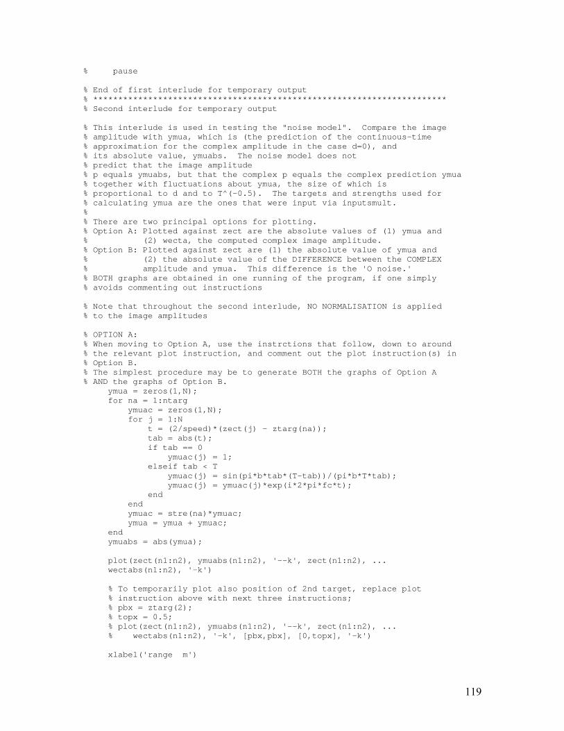
% pause % End of first interlude for temporary output % *********************************************************************** % Second interlude for temporary output % This interlude is used in testing the "noise model". Compare the image % amplitude with ymua, which is (the prediction of the continuous-time % approximation for the complex amplitude in the case d=0), and % its absolute value, ymuabs. The noise model does not % predict that the image amplitude % p equals ymuabs, but that the complex p equals the complex prediction ymua % together with fluctuations about ymua, the size of which is % proportional to d and to T^(-0.5). The targets and strengths used for % calculating ymua are the ones that were input via inputsmult. % % There are two principal options for plotting. % Option A: Plotted against zect are the absolute values of (1) ymua and % (2) wecta, the computed complex image amplitude. % Option B: Plotted against zect are (1) the absolute value of ymua and % (2) the absolute value of the DIFFERENCE between the COMPLEX % amplitude and ymua. This difference is the 'O noise.' % BOTH graphs are obtained in one running of the program, if one simply % avoids commenting out instructions % Note that throughout the second interlude, NO NORMALISATION is applied % to the image amplitudes % OPTION A: % When moving to Option A, use the instrctions that follow, down to around % the relevant plot instruction, and comment out the plot instruction(s) in % Option B. % The simplest procedure may be to generate BOTH the graphs of Option A % AND the graphs of Option B. ymua = zeros(1,N); for na = 1:ntarg ymuac = zeros(1,N); for j = 1:N t = (2/speed)*(zect(j) - ztarg(na)); tab = abs(t); if tab == 0 ymuac(j) = 1; elseif tab < T ymuac(j) = sin(pi*b*tab*(T-tab))/(pi*b*T*tab); ymuac(j) = ymuac(j)*exp(i*2*pi*fc*t); end end ymuac = stre(na)*ymuac; ymua = ymua + ymuac; end ymuabs = abs(ymua); plot(zect(n1:n2), ymuabs(n1:n2), '--k', zect(n1:n2), ... wectabs(n1:n2), '-k') % To temporarily plot also position of 2nd target, replace plot % instruction above with next three instructions; % pbx = ztarg(2); % topx = 0.5; % plot(zect(n1:n2), ymuabs(n1:n2), '--k', zect(n1:n2), ... % wectabs(n1:n2), '-k', [pbx,pbx], [0,topx], '-k') xlabel('range m')

119

ylabel('image amplitude') title('Image amp. (solid) and a kind of predicted mean (dashed)') pause % OPTION B: i.e. plot the difference % Actually the difference is plotted on an expanded scale, % the expansion factor being yexpand. Furthermore the rms value of the % 'O noise' (rms over the values of z used in plotting) is diplayed on the % screen as the variable anobrms % When moving to Option B, comment out the plot instruction(s) above, and % use the instructions that follow diff = abs(wecta - ymua); yexpand = 10; str1 = num2str(yexpand); % TEMPORARY SUPPRESSION OF ymuabs > 0.6 AND PLOTTING OF TWO VERTICAL % LINES % When suppressing, uncomment the 7 instructions immediately below, and % also replace plot instruction by the one that contains plottemp. % When reverting, reverse the procedure % ceiltemp = 0.6*ones(1, N); % plottemp = ymuabs; % plottemp(n1:n2) = min(ymuabs(n1:n2), ceiltemp(n1:n2)); % pb4 = zb4; % pb6 = zb6; % top4 = 0.69; % top6 = 0.69; % plot(zect(n1:n2), plottemp(n1:n2), '--k', zect(n1:n2), ... % yexpand*diff(n1:n2), '-k', [pb4,pb4], [0,top4], ':k', ... % [pb6,pb6], [0,top6], '--k') plot(zect(n1:n2), ymuabs(n1:n2), '--k', zect(n1:n2), ... yexpand*diff(n1:n2), '-k') % To temporarily plot also position of 2nd target, replace plot % instruction above with next three instructions; % pbx = ztarg(2); % topx = 0.5; % plot(zect(n1:n2), ymuabs(n1:n2), '--k', zect(n1:n2), ... % yexpand*diff(n1:n2), '-k', [pbx,pbx], [0,topx], '-k') xlabel('range m') ylabel('image amplitude') title(['Predicted mean and expanded difference (yexpand=', ... str1, ')']) % Compute rms 'O noise,' defined as rms value of diff anobrms = sqrt(sum((diff(n1:n2)).^2)/(n2-n1+1)); anobrms pause end % End of second interlude for temporary output % ************************************************************************ % ************ % Save first image (image from repeat = 1) for later plotting if multiple == 1 & repeat == 1 plot1 = nwectabs;

120

if tarsuppress == 1 plot11 = wectabs; end end % ************************************************************************* % This is the "main" plotting for the case multiple = 1 % Plot both images (images from repeat = 1 and repeat = 2) in one graph if repeat == 2 % Image for multiple=0 would have been nwectabs(nt) versus zect(nt). As % there are now two images to be plotted, essentially two vectors % nwectabs are plotted against a common vector zect % Plot image amplitudes versus position, the format of the plot being % either A or B below if (idiff == 0)|(idiff == 2) % A. Plot Image amplitude for first and second data sets. % Each of the two amplitudes is normalised so as to have a peak value of % unity. if tarsuppress == 0 plot(zect(n1:n2), plot1(n1:n2), '--k', zect(n1:n2), ... nwectabs(n1:n2), '-k', [pb1,pb1], [0,top1], ':k', ... [pb2,pb2], [0,top2], '-.k', [pb3,pb3], [0,top3], ... '--k', [pb4,pb4], [0,top4], '-k') xlabel('range m') ylabel('image amplitude (relative to peak)') title('First data set (dashed) Second (solid)') pause else % this is the case tarsuppress = 1. OPTION 1 (usually used): no % normalisation of image amplitude is applied % TEMPORARY SUPPRESSION OF wectabs > 0.4 % When suppressing, uncomment 3 instructiona and also change % wectabs to plottemp in plot instruction % When reverting, comment the 3 instructions and change % plot instruction back % ceiltemp = 0.4*ones(1, N); % plottemp = wectabs; % plottemp(n1:n2) = min(wectabs(n1:n2), ceiltemp(n1:n2)); plot(zect(n1:n2), plot11(n1:n2), '--k', zect(n1:n2), ... wectabs(n1:n2), '-k', [pb1,pb1], [0,top1], ':k', ... [pb2,pb2], [0,top2], '-.k', [pb3,pb3], [0,top3], ... '--k', [pb4,pb4], [0,top4], '-k') xlabel('range m') ylabel('image amplitude (unnormalised)') title('First data set (dashed) Second (solid)') pause % this is again the case tarsuppress = 1. OPTION 2 (not usually % used): A special normalisation of the image amplitude is applied % as follows. Total amplitude of the two images, over the plotted % region excluding the main lobe of the strong peak, is made the % same for both curves %n3 = floor(N/2 + 1 - delta + (fsamp/coeffsp)* ... % (ztarg(1) - speed/(2*B))); %n4 = ceil(N/2 + 1 - delta + (fsamp/coeffsp)* ... % (ztarg(1) + speed/(2*B)));

121

%sumplot1 = sum(plot1(n1:n3)) + sum(plot1(n4:n2)); %sumnw = sum(nwectabs(n1:n3)) + sum(nwectabs(n4:n2)); %plot2(n1:n2) = (sumplot1/sumnw)*nwectabs(n1:n2); %plot(zect(n1:n2), plot1(n1:n2), '--k', zect(n1:n2), ... % plot2(n1:n2), '-k', [pb1,pb1], [0,top1], ':k', ... % [pb2,pb2], [0,top2], '-.k', [pb3,pb3], [0,top3], ... % '--k', [pb4,pb4], [0,top4], '-k') %xlabel('range m') %ylabel('image amplitude (special normalisation)') %title('First data set (dashed) Second (solid)') %pause end end if (idiff == 1)|(idiff == 2) % B. Plot amplitude for first data set, and, on an expanded scale % and smoothed, plot [amplitude(second) - amplitude(first)] % Each of the two amplitudes is normalised so as to have a peak % value of unity--before any other operation is performed, including % the subtraction of one amplitude from the other. % iwidav is the number of elements in the smoothing window % iexpand is the factor by which expansion is to take place plot3 = plot1(n1:n2); plot4 = nwectabs(n1:n2); plot4 = maver(plot4 - plot3, iwidav); plot(zect(n1:n2), plot3, '--k', zect(n1:n2), ... iexpand*plot4, '-k', [pb1,pb1], [0,top1], ':k', ... [pb2,pb2], [0,top2], '-.k', [pb3,pb3], [0,top3], ... '--k', [pb4,pb4], [0,top4], '-k') xlabel('range m') ylabel('image amp p or [p(second) - p(first)] expanded and smoothed') title('First data set (dashed) Difference (expanded, smoothed) (solid)') pause end end % ************************************************************************* % Increment to allow multiple images repeat = repeat + 1; if multiple == 0 repeat = 1000; end % end of very long 'while' loop follows end more off disp('the end of the program has been reached')

122