Understanding the Missing Money Problem

NREL is a national laboratory of the U.S. Department of Energy Office of Energy Efficiency & Renewable Energy Operated by the Alliance for Sustainable Energy, LLC This report is available at no cost from the National Renewable Energy Laboratory (NREL) at www.nrel.gov/publications.

Contract No. DE-AC36-08GO28308

Modeling and Analysis of Wholesale Electricity Market Design: Understanding the Missing Money Problem December 2013 — January 2015 A. Papalexopoulos, C. Hansen, D. Perrino, and R. Frowd ECCO International, Inc. San Francisco, California

NREL Technical Monitor: Kara Clark

Subcontract Report NREL/SR-5D00-64255 May 2015

NREL is a national laboratory of the U.S. Department of Energy Office of Energy Efficiency & Renewable Energy Operated by the Alliance for Sustainable Energy, LLC This report is available at no cost from the National Renewable Energy Laboratory (NREL) at www.nrel.gov/publications.

Contract No. DE-AC36-08GO28308

National Renewable Energy Laboratory 15013 Denver West Parkway Golden, CO 80401 303-275-3000 • www.nrel.gov

Modeling and Analysis of Wholesale Electricity Market Design: Understanding the Missing Money Problem December 2013 — January 2015 A. Papalexopoulos, C. Hansen, D. Perrino, and R. Frowd ECCO International, Inc. San Francisco, California

NREL Technical Monitor: Kara Clark Prepared under Subcontract No. LGG-4-42314

Subcontract Report NREL/SR-5D00-64255 May 2015

This publication received minimal editorial review at NREL.

NOTICE

This report was prepared as an account of work sponsored by an agency of the United States government. Neither the United States government nor any agency thereof, nor any of their employees, makes any warranty, express or implied, or assumes any legal liability or responsibility for the accuracy, completeness, or usefulness of any information, apparatus, product, or process disclosed, or represents that its use would not infringe privately owned rights. Reference herein to any specific commercial product, process, or service by trade name, trademark, manufacturer, or otherwise does not necessarily constitute or imply its endorsement, recommendation, or favoring by the United States government or any agency thereof. The views and opinions of authors expressed herein do not necessarily state or reflect those of the United States government or any agency thereof.

This report is available at no cost from the National Renewable Energy Laboratory (NREL) at www.nrel.gov/publications.

Available electronically at SciTech Connect http:/www.osti.gov/scitech

Available for a processing fee to U.S. Department of Energy and its contractors, in paper, from:

U.S. Department of Energy Office of Scientific and Technical Information P.O. Box 62 Oak Ridge, TN 37831-0062 OSTI http://www.osti.gov Phone: 865.576.8401 Fax: 865.576.5728 Email: [email protected]

Available for sale to the public, in paper, from:

U.S. Department of Commerce National Technical Information Service 5301 Shawnee Road Alexandra, VA 22312 NTIS http://www.ntis.gov Phone: 800.553.6847 or 703.605.6000 Fax: 703.605.6900 Email: [email protected]

Cover Photos by Dennis Schroeder: (left to right) NREL 26173, NREL 18302, NREL 19758, NREL 29642, NREL 19795.

NREL prints on paper that contains recycled content.

http://www.osti.gov/scitech

http://www.osti.gov/

mailto:[email protected]

http://www.ntis.gov/

mailto:[email protected]

iii


List of Acronyms AC alternating current DC direct current ERCOT Electric Reliability Council of Texas LMP locational marginal price NREL National Renewable Energy Laboratory O&M operations and maintenance VG variable generation

iv


Executive Summary The National Renewable Energy Laboratory (NREL) has an interest in advancing the understanding of bulk power wholesale electricity market design issues related to capacity and flexibility in systems that have large amounts of variable generation (VG), mainly wind. NREL commissioned ECCO International, Inc. (ECCO), to study how high penetrations of VG will affect the outcomes of markets and incentives of the various pieces of the wholesale structure (energy, ancillary services, settlements, forward capacity) and what, if any, market design changes can improve incentives to ensure long-term power system reliability and efficiency.

This project examined the impact of renewable energy sources, which have zero incremental energy costs, on the sustainability of conventional generation. This “missing money” problem refers to market outcomes in which infra-marginal energy revenues in excess of operations and maintenance (O&M) costs are systematically lower than the amortized costs of new entry for a marginal generator. The problem is caused by two related factors: (1) conventional generation is dispatched less, and (2) the price that conventional generation receives for its energy is lower. This lower revenue stream may not be sufficient to cover both the variable and fixed costs of conventional generation. In fact, this study showed that higher wind penetrations in the Electric Reliability Council of Texas (ERCOT) system could cause many conventional generators to become uneconomic.

For continuity, all generator costs used in this paper were obtained from the 2013 U.S. Energy Information Administration report titled Updated Capital Cost Estimates for Utility Scale Electricity Generating Plants. This ensured consistent data. Also, the current ERCOT fleet was constructed throughout many decades, which makes it difficult to compare capital costs, and therefore these results indicate the costs that could be expected if the ERCOT fleet were replaced with new generators of the same type but using the latest advances and technologies.

Two cases were examined: (1) the base case, in which 13% of the energy was met with wind; and (2) the high wind case, in which 30% of the energy was met with wind. An additional 2.2% of the load in the high wind case could have been met with wind, but the energy was curtailed because of network congestion.

Generation was impacted by higher wind production in the following ways:

• Conventional (nuclear, coal, gas) generation was most negatively impacted.

o These units had dramatically reduced energy production, hours on, total revenue, and total profit.

o Conventional generation cleared more spinning reserve, but this is because it produced less energy. This was offset, however, by the large spinning reserve ancillary service price drop in the high wind case, from $8.71/MWh to $4.33/MWh.

• Overall system-wide generator fixed costs increased, because additional wind generators were being built and maintained.

o Overall fixed O&M costs rose from $2.4 billion to $3.2 billion.

v


o Similarly, overall levelized capital costs rose from $1.2 billion to $1.5 billion per year.

• Overall system-wide generator variable costs dropped because of the reduced production from conventional generators.

o Total system fuel costs dropped from $9.5 billion to $7.6 billion.

o Overall variable O&M costs dropped from $1.4 billion to $1.1 billion.

• The largest impact was on overall system-wide generator revenues and profits.

o Total system-wide revenue dropped from $16.8 billion to $11.4 billion because of the lower locational marginal prices (LMPs) and ancillary service prices.

o Total system profit (revenue – costs) dropped from $2.2 billion to -$2.2 billion, a reduction of $4.4 billion.

o Wind generator revenue increased marginally, from $1.74 billion to $1.82 billion, because of the depressed energy prices. With higher fixed costs, even wind generation lost money in the market in the high wind case. Note that this study did not consider production tax credits or other non-market incentives received by wind generators.

o The magnitude of the generator revenues and profits depends on the market structure. The prevailing market design is based on the marginal cost of production, and therefore it will be significantly impacted by the addition of resources that do not have incremental fuel costs.

o Note that conventional generation capacity in the high wind case was not adjusted. Economic theory is clear that additional generating capacity (wind or conventional) will lower prices and revenues. Further studies could examine the impact of a more optimal generation fleet, in which excess generating capacity would be minimized.

o The observed levels of congestion and curtailment in the high wind case in this study are plausible and should not have an unreasonable impact on the missing money problem. If all congestion and curtailment were eliminated, this would add (on average) slightly more than 1,000 MW of wind generation each hour. This would incrementally depress the average prices, revenues, and profits, but it would not materially change the primary findings. In other words, if additional transmission upgrades materialized, they would reduce the congestion component of the LMP prices and thus somewhat reduce in relative terms the LMP prices and slightly magnify the missing money problem.

This study quantified the impact of increased wind production on conventional generation in the ERCOT system. This missing money in organized electricity markets has the potential to inhibit new construction of conventional generation, which may in turn lead to a less reliable electric power system.

vi


Table of Contents 1 Introduction ........................................................................................................................................... 1 2 Missing Money Problem ...................................................................................................................... 2

2.1 Overview ....................................................................................................................................... 2 2.2 Impact of VG ................................................................................................................................. 2

3 Study Description ................................................................................................................................. 5 3.1 Input Data ...................................................................................................................................... 6 3.2 Input Data for the High Wind Case ............................................................................................... 6

4 Modeling Approach .............................................................................................................................. 9 4.1 Simulation Model .......................................................................................................................... 9 4.2 Wind Power Plant Model .............................................................................................................. 9

5 Benchmarking ..................................................................................................................................... 11 5.1 Description .................................................................................................................................. 11 5.2 Issues ........................................................................................................................................... 11 5.3 Adjustments ................................................................................................................................. 12 5.4 Sample Results ............................................................................................................................ 12

5.4.1 Price Duration Curves .................................................................................................... 12 5.4.2 Hourly Price Comparisons ............................................................................................. 13

6 Results and Analysis ......................................................................................................................... 17 6.1 Hub Prices ................................................................................................................................... 17

6.1.1 Average Hourly Hub Prices ........................................................................................... 17 6.1.2 Average Monthly Hub Prices ......................................................................................... 21

6.2 Generator Results ........................................................................................................................ 23 6.2.1 Generator Costs Breakdown ........................................................................................... 23 6.2.2 Generator Profits ............................................................................................................ 27

6.3 Wind Curtailment ........................................................................................................................ 30 7 Binding Constraints ........................................................................................................................... 33 8 Conclusion .......................................................................................................................................... 37 References ................................................................................................................................................. 39

vii


List of Figures Figure 1. ERCOT transmission network upgrades ....................................................................................... 7 Figure 2. Average monthly wind production profile used in the high wind case ....................................... 10 Figure 3. Comparison of annual price duration curves ............................................................................... 12 Figure 4. Comparison of simulated prices to actual prices for September 19, 2013 .................................. 13 Figure 5. Comparison of simulated prices to historical prices for June 5, 2013 ......................................... 14 Figure 6. Comparison of simulated prices to actual prices for July 22, 2013 ............................................. 15 Figure 7. Comparison of simulated prices to actual prices for September 6, 2013 .................................... 16 Figure 8. Average hourly hub prices for the entire study year—base case ................................................. 18 Figure 9. Average hourly hub prices for the entire study year—high wind case ........................................ 19 Figure 10. Average hourly hub prices for the entire study year—case comparison ................................... 20 Figure 11. Average monthly hub prices for the entire study year—base case ............................................ 21 Figure 12. Average monthly hub prices for the entire study year—high wind case ................................... 22 Figure 13. Average monthly hub prices for the entire study year—case comparison ................................ 23 Figure 14. Monthly wind curtailments (MWh)—base case compared to high wind case .......................... 32

List of Tables Table 1. New Wind Power Plant Profiles ..................................................................................................... 7 Table 2. Costs Used in the Modeling ............................................................................................................ 8 Table 3. Assumed Generator Costs for ERCOT ......................................................................................... 24 Table 4. Generator Costs Breakdown (U.S. $) for the Entire Study Year—Base Case .............................. 25 Table 5. Generator Costs Breakdown (U.S. $) for the Entire Study Year—High Wind Case .................... 26 Table 6. Generator Summary for the Entire Study Year—Base Case ........................................................ 27 Table 7. Generator Summary for the Entire Study Year—High Wind Case .............................................. 28 Table 8. Generator Summary for the Entire Study Year—Difference between Cases (%) ........................ 29 Table 9. Top 10 Curtailed Wind Generators—Base Case .......................................................................... 30 Table 10. Top 10 Curtailed Wind Generators—High Wind Case .............................................................. 31 Table 11. Top 20 Binding Constraints (Shadow Price > $100)—Base Case .............................................. 34 Table 12. Top 20 Binding Constraints (Shadow Price > $100)—High Wind Case .................................... 35

1


1 Introduction The National Renewable Energy Laboratory (NREL) retained ECCO International, Inc. (ECCO), to analyze the “missing money” problem in wholesale energy markets arising from the substantial penetration of variable generation (VG) such as renewable energy resources, especially wind, into the energy mix. Missing money refers to market outcomes in which infra-marginal energy revenues in excess of operations and maintenance (O&M) costs are systematically lower than the amortized costs of new entry for a marginal generator. The purpose of this project was to study the impact of wind on the long-term revenue adequacy problem of independent system operator markets and the long-term incentives of resources that are needed to provide capacity and flexibility to the electric power system. A related objective was to propose a set of wholesale market design changes to ensure that revenue adequacy is addressed. NREL actively analyzes bulk power system wholesale market design and performance in the presence of large amounts of wind and solar generation. This work complements and expands upon these efforts.

Wind and solar generation have several characteristics that uniquely impact wholesale power markets. These resources increase the variability and uncertainty on the power system, which requires additional flexibility. The combination of variability, uncertainty, and the near-zero variable cost of renewable energy sources may result in generally lower but more volatile energy prices, higher ancillary service prices, and, depending on the market design, higher forward capacity prices. There is significant interest in the extent to which these changes will impact particular market designs and what, if any, market design modifications will be required to achieve the desired reliable and efficient power system operations.

For this study, ECCO applied its advanced proprietary energy simulation software platform ProMaxLT to the Electric Reliability Council of Texas (ERCOT) market to quantify the missing money problem. Based on prior work, it seems that wholesale energy-only markets may not provide sufficient revenue and certainty to support the new investments in generating capacity necessary to produce the required levels of resource adequacy and reliability. We examined and quantified the extent of this issue at various high levels of VG penetrations. This report provides analytical results about the potential outcomes on profit and revenue of different technologies for the ERCOT market. In addition, it presents quantitative results on the extent to which current market designs provide the opportunity for generating resources to recover both fixed and variable costs and can continue to incentivize resources to contribute to long-term system reliability.

2


2 Missing Money Problem 2.1 Overview To analyze the impact of VG, such as wind, on long-term revenue adequacy and the long-term incentives of resources that are needed to provide capacity and flexibility to the electric power system, we focused on a high-penetration renewable supply scenario to illustrate how revenue may or may not achieve adequacy based on the supply mix under current market rules. We defined a base case study and a set of changes with predetermined penetration levels of intermittent supply using the unique software platform ProMaxLT to deploy a full and detailed network model of ERCOT.

2.2 Impact of VG The electricity network can be generally divided into two subsystems: (1) the transmission (or bulk) system and (2) the distribution system. These networks are predominantly distinguished by different voltage levels. The transmission system primarily delivers electricity generated at central stations to locations close to load centers. In North America, the transmission system usually operates at voltage levels from 69 kV to 765 kV, and it is highly interconnected. The transmission system also has significant levels of monitoring, automation, and control.

The distribution system delivers electricity from transmission substations stepped down to lower voltages to customers. The distribution system typically operates at voltage levels ranging from 69 kV to 120 V. It is predominantly radial in structure, and it does not have the same level of automation as the transmission system, although this is changing with the onset of many “smart-grid” initiatives.

The introduction of VG can modify or exacerbate resource adequacy and revenue sufficiency in electric power systems. First, it is important to understand that VG’s contribution to resource adequacy is very different than that of conventional generation. Although forced outage rates of an entire collection of wind turbines or photovoltaic cells are very rare and not likely to significantly contribute to their unavailability, these resources can be quite variable because of changing weather patterns. Thus, VG increases the amount of variability and uncertainty on power systems, which can therefore require an increased need for flexibility. Although certain changes to short-term energy and ancillary service markets may be needed to ensure that the flexibility that is available is provided, these changes may not guarantee that sufficient flexibility is built or available in the first place. This could lead to the need for new ways to perform resource adequacy evaluations. Finally, the costs of VG are almost entirely fixed capital costs rather than variable operating costs. This can bring energy prices down while potentially increasing (or keeping constant) the total variable and fixed costs in the power system. This could lead to further reliance on markets or incentives other than the energy market to ensure that the resources needed for long-term reliability can recover both variable and fixed capital costs—i.e., the need for capacity markets and revenues increases.

VG increases the variability and uncertainty of the electric power

system, reduces spot energy prices, and therefore exacerbates the capacity assurance problem.

3


Actual experience with operational markets with high penetrations of VG and renewable energy sources indicates that the low marginal costs of these resources substantially decrease market prices and thus reduce the revenue of all suppliers in the energy market. This may add to revenue insufficiency and prevent suppliers from recovering variable and fixed costs. In addition to reducing electricity prices, VG displaces other resources via the merit-order effect, such that capacity factors for other generator types are also reduced. The question is how to ensure revenue sufficiency based on the combination of lower energy prices and lower capacity factors of existing plants. It may be possible that although the majority of prices are being depressed the occasional high-price spikes will increase and help to capture needed revenue. However, this may depend on price caps, market mitigation procedures, and the levels of administratively set scarcity pricing. Finally, the existence and design of forward capacity markets can have a large impact on the level of revenue sufficiency.

In part, this study examined whether there is any measurable impact by VG on the existing missing money problem and, if so, attempted to quantify how much. Wind and solar are two key VG resources that can clearly have a major impact on the missing money problem.

Wind power plants are typically located in areas where wind resources are plentiful and can satisfy certain requirements. Most onshore wind power plants are located in rural areas where the transmission system voltages typically range from 69 kV to 161 kV. The nominal terminal voltages at the wind turbines range from 575 V to 4,160 V, depending on the turbine ratings. The unit transformer at each wind turbine steps up the voltage and feeds power into a collector system that operates at voltages ranging from 12.5 kV to 34.5 kV. The high-side node of the collector system is then connected to the main substation transformer for the wind power plant, which again steps up the voltage to the desired level and connects the wind power plant to the transmission system in the geographical vicinity.

Distributed photovoltaic resources that have inverters produce alternating current (AC) output at the desired voltage. In residential neighborhoods, these connect the residences directly to the utility supply point. Utilities around the country have established standards for these connections to minimize the significant safety risks of the bidirectional flow in existing residential supply circuits if the customer sells power back to the utility. Commercial or utility-scale photovoltaic units have similar interconnection requirements. In most instances, however, they interconnect with the distribution system at slightly higher voltage levels than residential photovoltaic units, depending on their location and ratings.

Central solar thermal resources, on the other hand, have significantly higher ratings and connect to the transmission grid at high voltage levels ranging from 230 kV to 345 kV.

The increased penetration of renewable energy sources is beginning to significantly alter the traditional approach to operation and unit commitment processes. The variability of renewable resources requires measures to accommodate fast generation changes (e.g., from a few seconds to hours during transition periods) and account for sufficient commitment and dispatch of ancillary services to guarantee the reliability of the system in the event that a renewable resource

4


suddenly becomes unavailable—for example, when the wind lightens or stops altogether or previously unanticipated cloud cover appears and significantly reduces photovoltaic output.1

To manage the uncertainty of these resources while making use of their many positive attributes, independent system operators around the world are making changes to their energy and ancillary service markets. At the same time, operators are adjusting to the new realities and becoming adept at monitoring and forecasting weather pattern changes.

1 See https://www.nae.edu/Publications/Bridge/TheElectricityGrid/18587.aspx.

https://www.nae.edu/Publications/Bridge/TheElectricityGrid/18587.aspx

5


3 Study Description The following specific tasks were executed during the course of this project.

ECCO prepared base case models for the year 2016 according to ERCOT data available through their planning Web site.2 It included generation and load data, detailed transmission data, and renewable energy source generation data. As required, these models were augmented with planned changes to the transmission system to match the corresponding study year.

ECCO ran the representative base case and then the change case that contained the generation updates as identified for the renewable assets modeled and agreed to by NREL, as follows:

• Case-1—Base case year

• Case-2—Change case year with 30% penetration of renewables

In addition, ECCO analyzed critical data that assisted in leading to a more “fact-based” solution for consideration, including the

• ERCOT generation mix by type and age of the generation facilities

• Types of generation suppliers present in the ERCOT market

• Expected growth in load by type and category

• Expected near-term and long-term weather conditions

• Current volume of renewable resources by type and storage technologies by type that are online and planned in the near term and long term

• Houston Ship Channel Index natural gas prices since the inception of the Nodal market

• Historical bid prices from the ERCOT market for all plant types, including wind

• Real-time and day-ahead LMPs since the inception of the nodal market at all ERCOT generation nodes.

To determine the extent of the missing money, we conducted a counterfactual simulation of unit commitment and real-time dispatch that dispatched a generic unit at each of the generation nodes against the historical day-ahead and real-time LMP at that node under the assumption that the unit offered its supply at true marginal cost and, if dispatched, was paid the LMP. The marginal cost was calculated by assuming a specific heat rate and fuel cost set to the Houston Ship Channel Index natural gas price at the time the power was supplied. The annual net income to the generic unit was calculated as a function of heat rate ranging from 7,000 Btu/kWh to 22,000 Btu/kWh in increments of 1,000 Btu/kWh. Start-up and no-load costs were assumed based on industry averages using Energy Information Administration data. These costs were incorporated into the simulation along with a daily make-whole assumption, which reflected ERCOT market rules. The objective of this simulation was to determine the threshold heat rate, if any, at which a unit’s net

2 See http://www.ercot.com/gridinfo/planning/index.html. As of November 15, 2014 the Planning and Operation Information (POI) website has been retired with its content moved to the Market Information System (MIS). See http://www.ercot.com/content/meetings/rpg/keydocs/2014/0819/POI_to_MIS_Transition.ppt.

http://www.ercot.com/gridinfo/planning/index.html

http://www.ercot.com/content/meetings/rpg/keydocs/2014/0819/POI_to_MIS_Transition.ppt

6


income (under truthful bidding assumptions) would cover the annual costs of new entry, which would then be determined based on data from the Energy Information Administration.

The above simulation studies were repeated under a variety of assumptions regarding load growth, renewable penetration, demand response policies, and variation in LMP patterns as a result of transmission expansion, and the results were analyzed.

3.1 Input Data The following information was obtained from ERCOT’s planning website.3

1. The hourly load forecasts were obtained from http://planning.ercot.com/content/25446.4 These were scaled for consistency with more recent annual load forecasts.

2. The network models and contingency constraints were obtained from http://planning.ercot.com/content/28448.5

3. The bids were obtained directly from ERCOT via a disclosure request. The real-time bids were used in the market simulations, but the day-ahead bids included in the disclosure were co-optimized with the financial transmission rights market and not suitable for this type of simulation.

4. The unit outage state was also obtained via the disclosure.

3.2 Input Data for the High Wind Case For the study, we assumed that all wind power plants would bid with negative prices.

Wind profiles for new wind power plants in the high wind case were obtained by using NREL’s Wind Toolkit.6 These wind power plants were located in zones according to the latitude and longitude of the facilities provided. The generation profiles were then assigned to 345-kV buses in each zone, as described below and summarized in Table 1.

1. The buses were chosen so that there would be sufficient local network capability to handle their full output without local congestion.

2. Explicit plant sizes were not imposed on these wind power plants, because the maximum values used in the simulations were downloaded from the tool kit.

3. The network model in the high wind case was augmented with planned network additions to accommodate wind resources according to ERCOT’s Panhandle Renewable Energy Zone (PREZ) Study Report (2014).

4. The Panhandle stability limit was set to 7,500 MW in the high wind case.

5. Per the Panhandle report, additional 345-kV lines were added to the following locations:

A. Oklaunion-Bowman B. Ogallala–Long Draw C. Windmill–Edith Clarke

3 Please refer to footnote 1 on page 5. 4 Please refer to footnote 1 on page 5. 5 Please refer to footnote 1 on page 5. 6 See http://developer.nrel.gov/docs/wind/wind-toolkit-extract/.

http://planning.ercot.com/content/25446

http://planning.ercot.com/content/28448

http://developer.nrel.gov/docs/wind/wind-toolkit-extract/

7


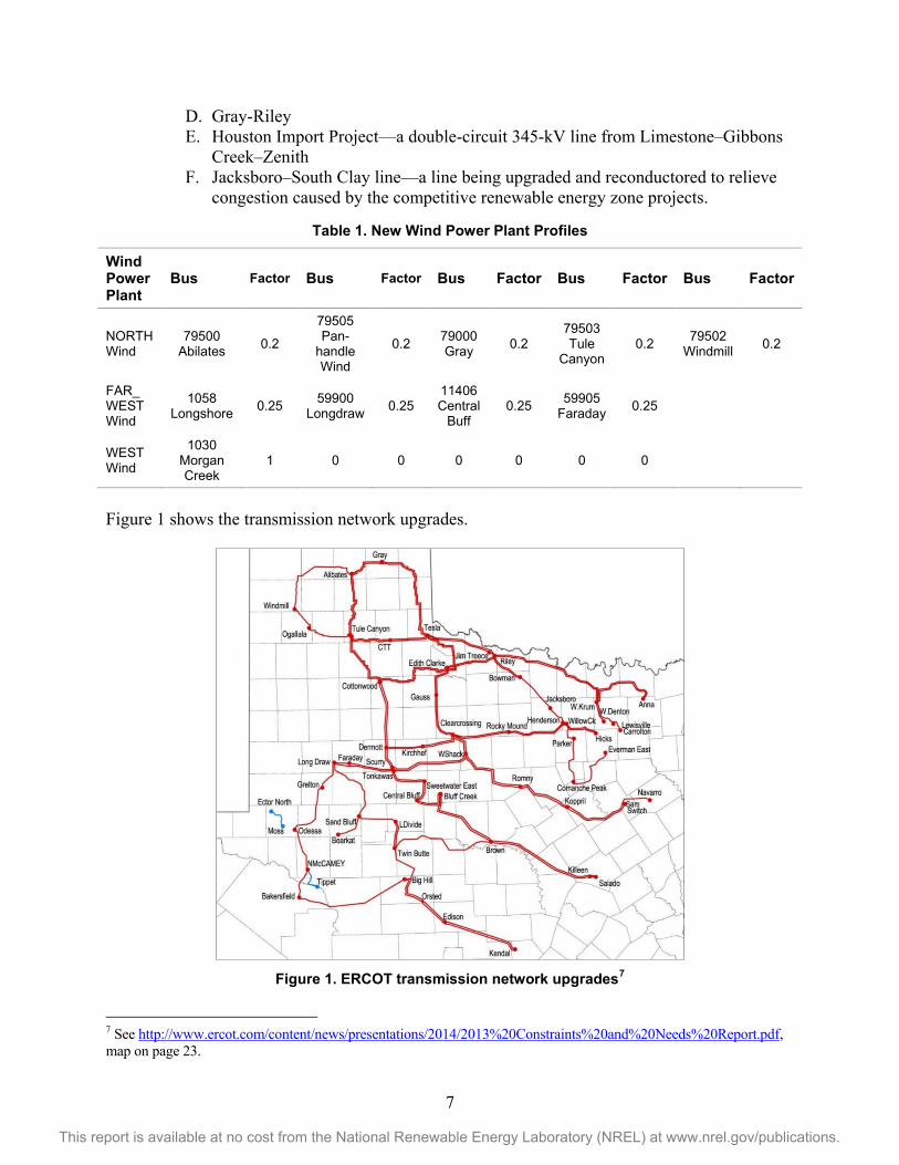
D. Gray-Riley E. Houston Import Project—a double-circuit 345-kV line from Limestone–Gibbons

Creek–Zenith F. Jacksboro–South Clay line—a line being upgraded and reconductored to relieve

congestion caused by the competitive renewable energy zone projects.

Table 1. New Wind Power Plant Profiles

Wind Power Plant

Bus Factor Bus Factor Bus Factor Bus Factor Bus Factor

NORTH Wind

79500 Abilates 0.2

79505 Pan-

handle Wind

0.2 79000 Gray 0.2

79503 Tule

Canyon 0.2 79502

Windmill 0.2

FAR_ WEST Wind

1058 Longshore 0.25 59900

Longdraw 0.25 11406 Central

Buff 0.25 59905

Faraday 0.25

WEST Wind

1030 Morgan Creek

1 0 0 0 0 0 0

Figure 1 shows the transmission network upgrades.

Figure 1. ERCOT transmission network upgrades7

7 See http://www.ercot.com/content/news/presentations/2014/2013%20Constraints%20and%20Needs%20Report.pdf, map on page 23.

http://www.ercot.com/content/news/presentations/2014/2013%20Constraints%20and%20Needs%20Report.pdf

8


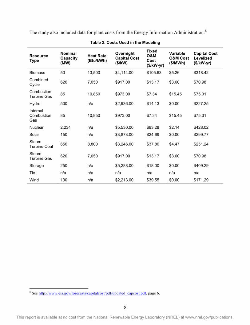
The study also included data for plant costs from the Energy Information Administration.8

Table 2. Costs Used in the Modeling

Resource Type

Nominal Capacity (MW)

Heat Rate (Btu/kWh)

Overnight Capital Cost ($/kW)

Fixed O&M Cost ($/kW-yr)

Variable O&M Cost ($/MWh)

Capital Cost Levelized ($/kW-yr)

Biomass 50 13,500 $4,114.00 $105.63 $5.26 $318.42

Combined Cycle 620 7,050 $917.00 $13.17 $3.60 $70.98

Combustion Turbine Gas 85 10,850 $973.00 $7.34 $15.45 $75.31

Hydro 500 n/a $2,936.00 $14.13 $0.00 $227.25

Internal Combustion Gas

85 10,850 $973.00 $7.34 $15.45 $75.31

Nuclear 2,234 n/a $5,530.00 $93.28 $2.14 $428.02

Solar 150 n/a $3,873.00 $24.69 $0.00 $299.77

Steam Turbine Coal 650 8,800 $3,246.00 $37.80 $4.47 $251.24

Steam Turbine Gas 620 7,050 $917.00 $13.17 $3.60 $70.98

Storage 250 n/a $5,288.00 $18.00 $0.00 $409.29

Tie n/a n/a n/a n/a n/a n/a

Wind 100 n/a $2,213.00 $39.55 $0.00 $171.29

8 See http://www.eia.gov/forecasts/capitalcost/pdf/updated_capcost.pdf, page 6.

http://www.eia.gov/forecasts/capitalcost/pdf/updated_capcost.pdf

9


4 Modeling Approach 4.1 Simulation Model ECCO used its proprietary energy market simulation software package ProMaxLT9 to perform the modeling and simulation runs for these studies.

ECCO’s ProMaxLT software platform was developed during the course of the last 10 years. It deploys a mixed integer programming–based security constrained unit commitment and an advanced linear programming–based security constrained economic dispatch with a full and detailed transmission network model. The transmission model can have either AC or direct current (DC) power flow, which iterates with the mixed integer programming commitment and dispatch engine to explicitly represent the network constraints and calculate meaningful shadow prices from the dual variables of the binding constraints. Contingency constraints are explicitly enforced using sensitivities derived from the network impedance matrices so that tens of thousands of contingencies can be enforced in the dispatch and their corresponding shadow prices can be calculated.

ECCO used the ProMaxLT day-ahead market simulation platform to compute hourly LMPs for the study scenarios using a full mixed integer programming formulation iterating with the DC power flow in the same manner as performed by the ERCOT day-ahead market clearing process. All transmission constraints were enforced so that curtailment of wind and other plants would occur when insufficient network capacity was available.

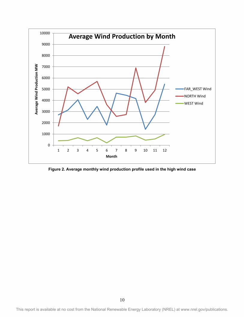
4.2 Wind Power Plant Model Wind power plants were modeled as variable plants with zero start-up costs and negative bid prices. Minimum up and down times were not enforced. Hourly wind profiles for the existing plants were obtained from ERCOT’s expansion wind data.10

NREL’s Wind Toolkit was deployed to create the wind profiles in the high wind case according to the following process:

1. Each potential plant was allocated to a particular ERCOT weather zone according to its latitudinal and longitudinal coordinates.

2. The wind power plants were sorted in descending order of average production.

3. Hourly wind profiles were read for each plant until the desired 30% energy production targets were met.

4. The MW value from the Wind Toolkit was used as the maximum limit for each plant for each interval. These plants were allowed to vary between zero and the maximum obtained from the profile with a bid price of -$25/MWh. This bid price was the most commonly used setting for wind generators with the production tax credit (PTC). Wind power plants were not allowed to participate in the ancillary services market.

9See http://www.eccointl.com/our-services/reliability-assessment-studies.html. 10 See http://www.ercot.com/content/committees/other/lts/keydocs/2013/expansion_wind_unit_data_used_in_LTS.xls.

http://www.eccointl.com/our-services/reliability-assessment-studies.html

http://www.ercot.com/content/committees/other/lts/keydocs/2013/expansion_wind_unit_data_used_in_LTS.xls

10


Figure 2. Average monthly wind production profile used in the high wind case

0

1000

2000

3000

4000

5000

6000

7000

8000

9000

10000

1 2 3 4 5 6 7 8 9 10 11 12

Aver

age

Win

d Pr

oduc

tion

MW

Month

Average Wind Production by Month

FAR_WEST Wind

NORTH Wind

WEST Wind

11


5 Benchmarking The benchmarking process is fairly standard across industries. The objective is to calibrate and validate software models by deploying past data and then use the calibrated software to execute various studies. In this project, the objective was to be able to reliably and accurately calculate LMPs for the ERCOT energy market using actual past prices.

Toward that end, ECCO collected the data required, including the published LMP data from ERCOT market runs along with historical bids and publicly available offer data. Based on past experience, the bidding process of market participants can be simulated in two ways:

1. Use marginal-based bids and offers (heat rate times spot fuel price) for the generating units participating in the market.

2. Use historical bids and publicly available offers.

In most markets, it has been our observation that participants do not bid marginal-based offers; however, we needed to verify whether this is valid for ERCOT. Thus, ECCO executed the first option, and if the results were not acceptable, ECCO executed the second option as well.

5.1 Description Prior to performing the analysis, benchmarking was performed to ensure that the results provided a realistic and plausible simulation of nodal prices in the ERCOT market. Actual historical 2013 loads were used with real-time bids and unit outage statuses obtained via the public disclosure process.

The primary measure of the benchmarking exercise is the cleared hub prices for the simulated and actual cases. A complete 8,760-hour simulation was performed for all of 2013 using actual loads and real-time bids downloaded from the ERCOT Web site. Benchmarking was performed by comparing the simulated hub prices to the historical hub prices provided on the site.

5.2 Issues The benchmarking process using the first option (i.e., heat rate times fuel price and heuristically generated outage schedules) did not yield sufficiently accurate comparisons between the simulated and actual results. We believe these differences were because of the following:

1. As expected, based on a review of actual bid and offer data for the ERCOT day-ahead market, it was observed that ERCOT market participants do not normally bid on heat rate times the spot fuel price. Market participants typically have long-term fuel supply contracts that dictate the prices they would pay for fuel, and therefore their bidding behavior is not always driven by the spot fuel price. The terms of these fuel supply contracts are generally confidential. This observation is consistent with our conclusions about other markets.

2. ERCOT market participants can utilize bilateral contracts with load-serving entities that govern the actual price paid for energy. These market participants often bid lower prices to make sure that their contract position clears.

12


3. Unit outage schedules can substantially influence simulated prices. If historical outage schedules are not available, then these schedules need to be generated manually or by some other automated heuristic process. In benchmarking, this can lead to substantial differences between the simulated and actual prices.

5.3 Adjustments To address these difficulties with price benchmarking, ECCO executed the second option. Toward that end, actual historical bids and offers and associated outage schedules were obtained via a disclosure request to ERCOT, which provided the entire set of 2013 real-time and day-ahead bids and outage schedules. These data were used in the simulations in this study.

ECCO deployed the available historic bids and offers and mapped them through reverse engineering onto the ERCOT transmission grid and backcasted the ERCOT market runs to predict and match the resulting LMPs to the actual published LMPs.

5.4 Sample Results The sections below provide samples illustrating the results obtained during the benchmarking process using the second option.

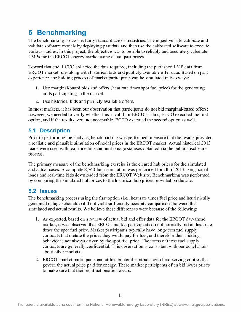
5.4.1 Price Duration Curves Figure 3 illustrates the results of the benchmarking calculations for the West hub prices as a price duration curve. This graph is a cumulative probability distribution of the simulated and historical hub prices.

Figure 3. Comparison of annual price duration curves

13


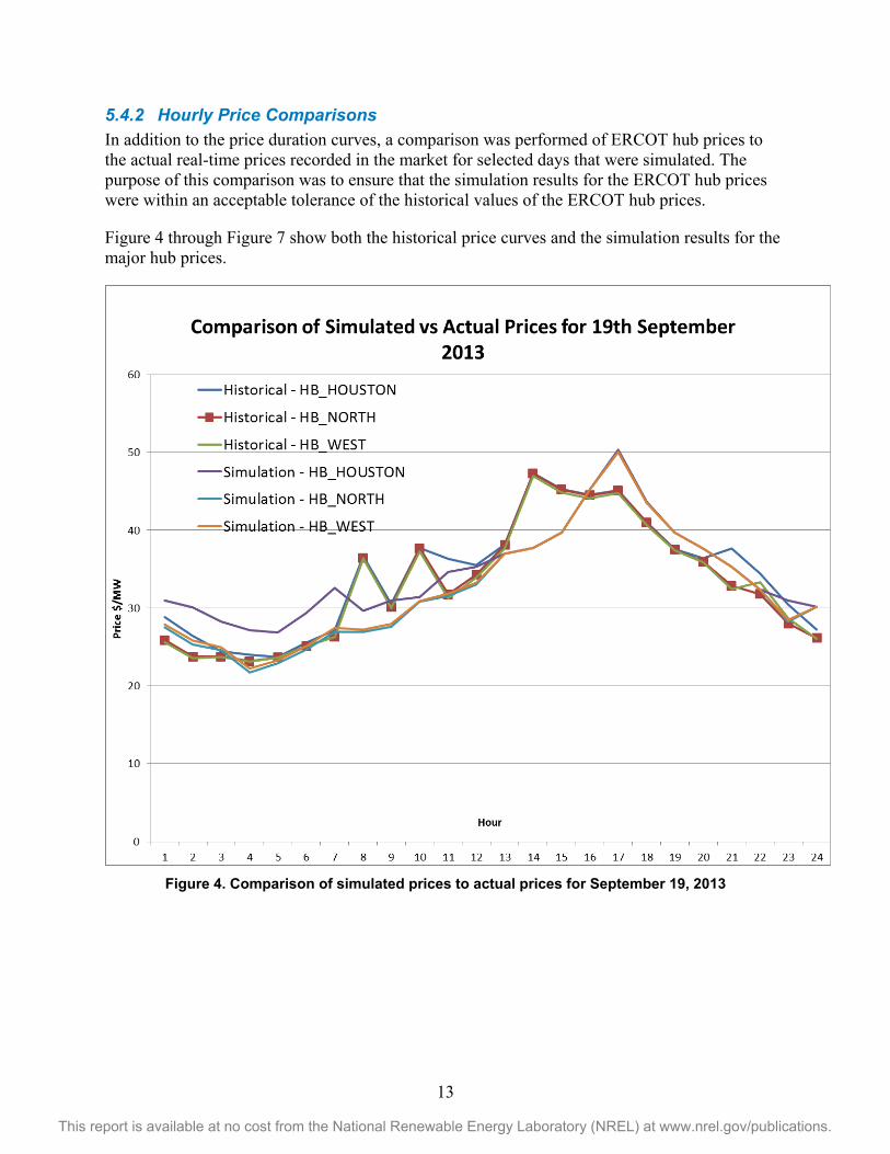
5.4.2 Hourly Price Comparisons In addition to the price duration curves, a comparison was performed of ERCOT hub prices to the actual real-time prices recorded in the market for selected days that were simulated. The purpose of this comparison was to ensure that the simulation results for the ERCOT hub prices were within an acceptable tolerance of the historical values of the ERCOT hub prices.

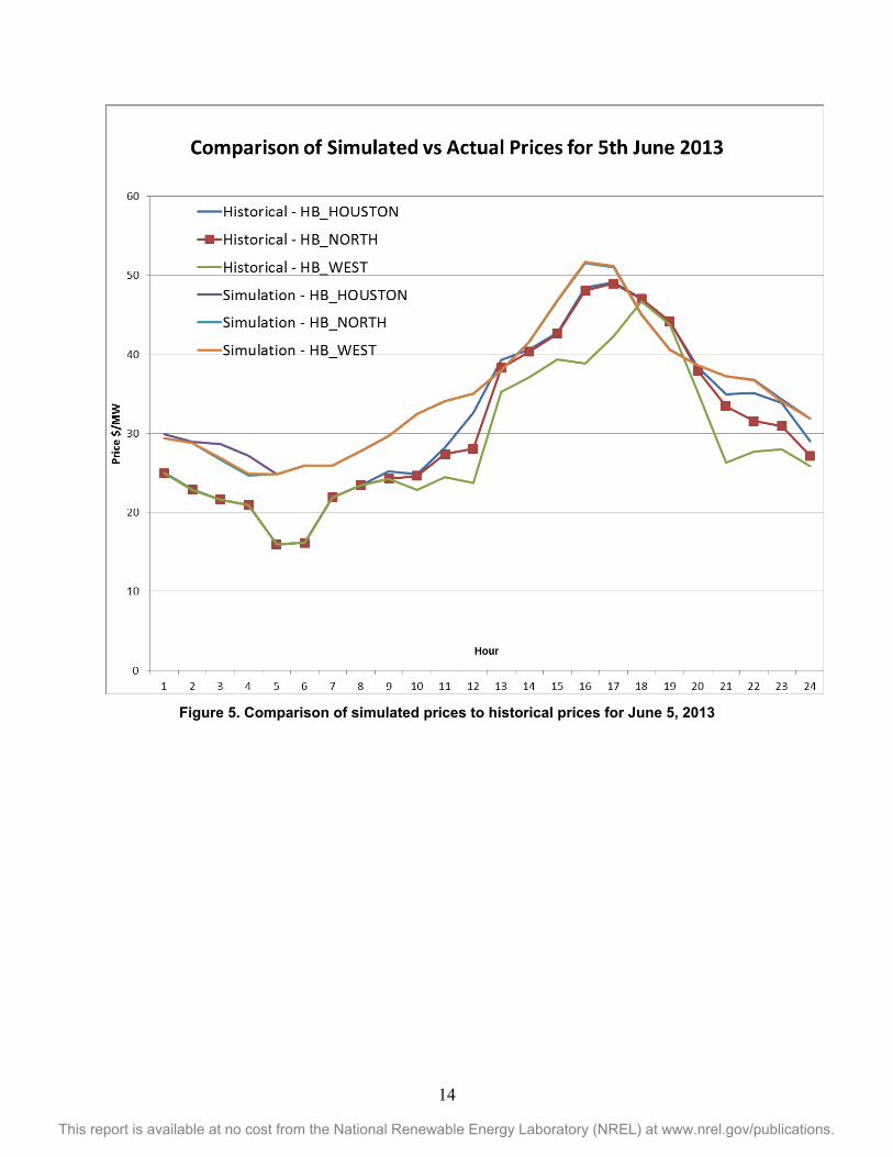
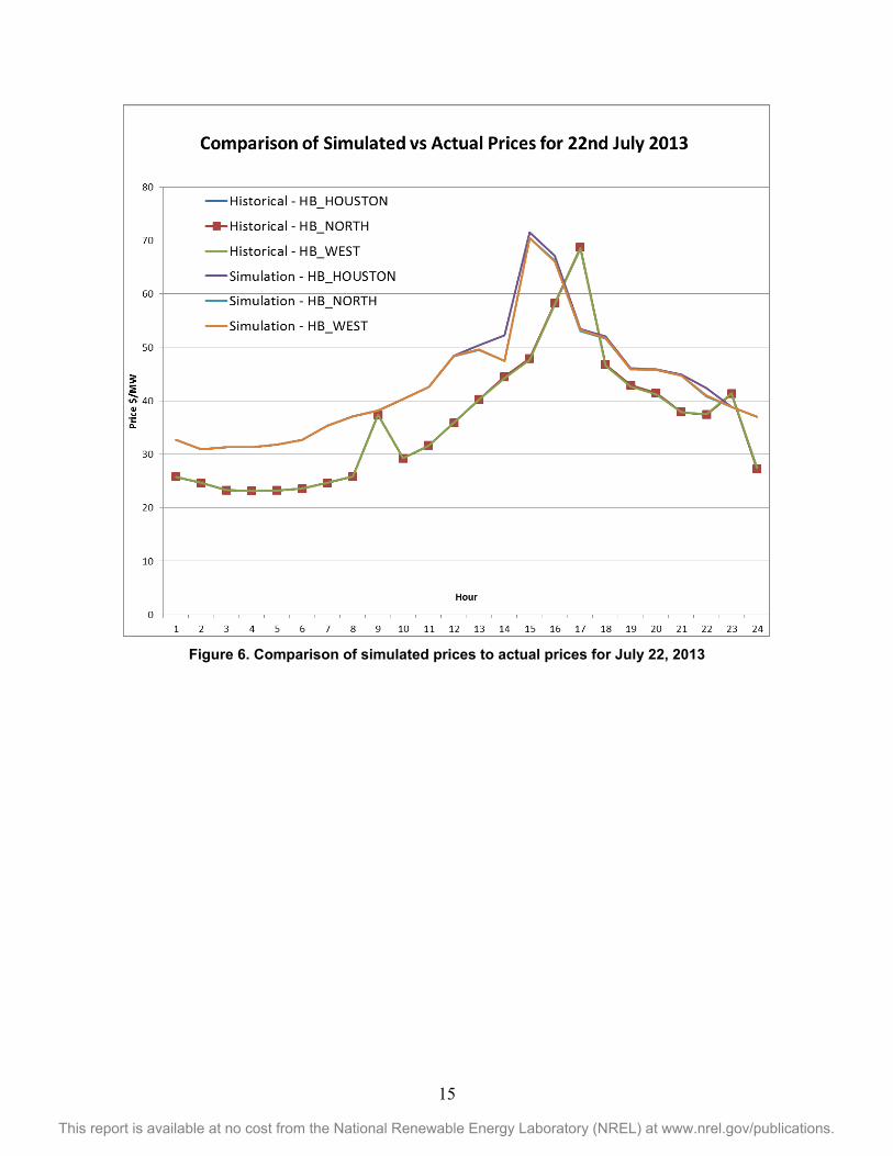
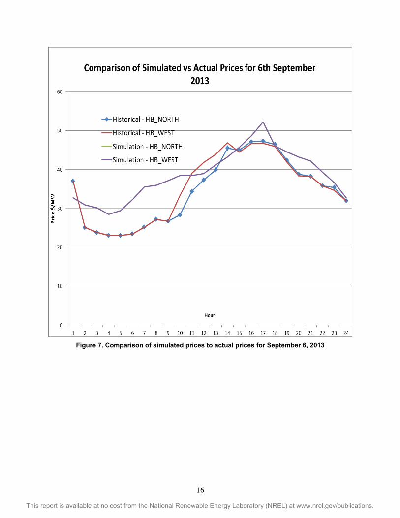
Figure 4 through Figure 7 show both the historical price curves and the simulation results for the major hub prices.

Figure 4. Comparison of simulated prices to actual prices for September 19, 2013

14


Figure 5. Comparison of simulated prices to historical prices for June 5, 2013

15


Figure 6. Comparison of simulated prices to actual prices for July 22, 2013

16


Figure 7. Comparison of simulated prices to actual prices for September 6, 2013

17


6 Results and Analysis This section presents the results and analysis of the base case and the high wind case and considers the following factors:

• Hub prices

o Hourly averages

o Monthly averages

• Generator economics

o Cost assumptions

o Cost components

o Energy and ancillary service awards

o LMPs, revenue, and profits

• Wind curtailments

• Network congestion.

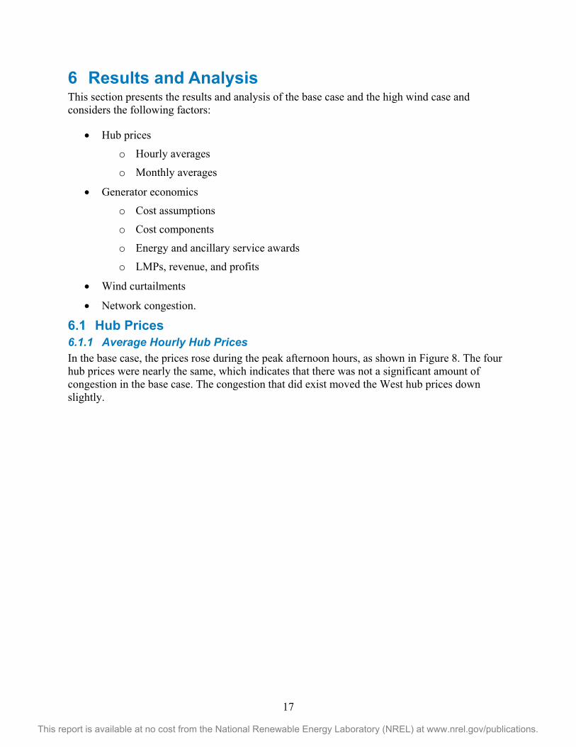
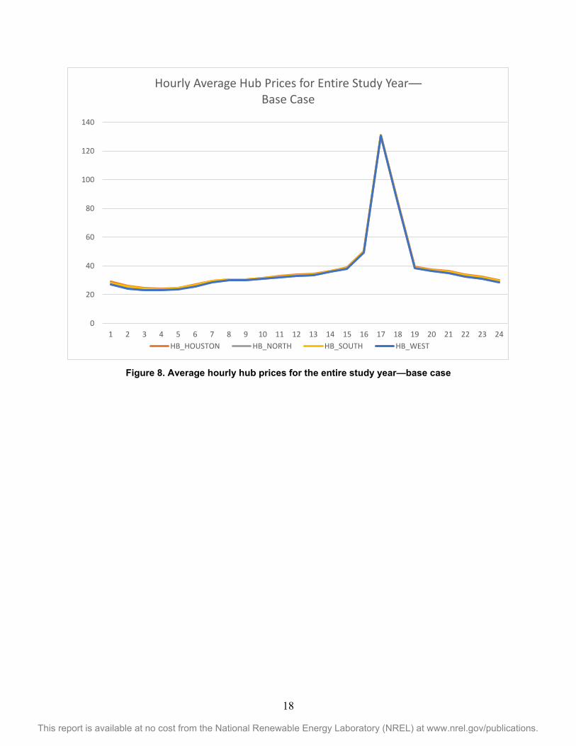
6.1 Hub Prices 6.1.1 Average Hourly Hub Prices In the base case, the prices rose during the peak afternoon hours, as shown in Figure 8. The four hub prices were nearly the same, which indicates that there was not a significant amount of congestion in the base case. The congestion that did exist moved the West hub prices down slightly.

18


Figure 8. Average hourly hub prices for the entire study year—base case

0

20

40

60

80

100

120

140

1 2 3 4 5 6 7 8 9 10 11 12 13 14 15 16 17 18 19 20 21 22 23 24

Hourly Average Hub Prices for Entire Study Year— Base Case

HB_HOUSTON HB_NORTH HB_SOUTH HB_WEST

19


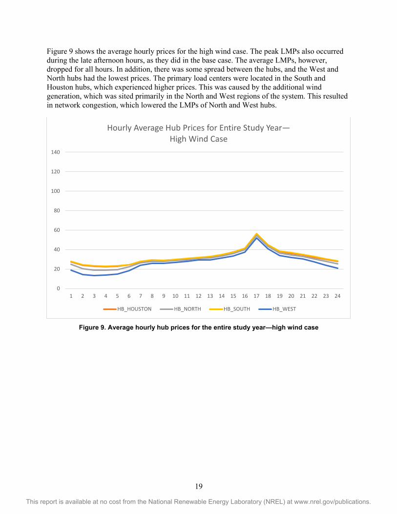
Figure 9 shows the average hourly prices for the high wind case. The peak LMPs also occurred during the late afternoon hours, as they did in the base case. The average LMPs, however, dropped for all hours. In addition, there was some spread between the hubs, and the West and North hubs had the lowest prices. The primary load centers were located in the South and Houston hubs, which experienced higher prices. This was caused by the additional wind generation, which was sited primarily in the North and West regions of the system. This resulted in network congestion, which lowered the LMPs of North and West hubs.

Figure 9. Average hourly hub prices for the entire study year—high wind case

0

20

40

60

80

100

120

140

1 2 3 4 5 6 7 8 9 10 11 12 13 14 15 16 17 18 19 20 21 22 23 24

Hourly Average Hub Prices for Entire Study Year— High Wind Case


20


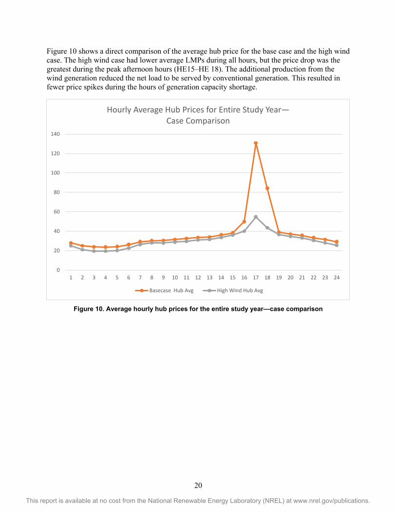
Figure 10 shows a direct comparison of the average hub price for the base case and the high wind case. The high wind case had lower average LMPs during all hours, but the price drop was the greatest during the peak afternoon hours (HE15–HE 18). The additional production from the wind generation reduced the net load to be served by conventional generation. This resulted in fewer price spikes during the hours of generation capacity shortage.

Figure 10. Average hourly hub prices for the entire study year—case comparison

0

20

40

60

80

100

120

140

1 2 3 4 5 6 7 8 9 10 11 12 13 14 15 16 17 18 19 20 21 22 23 24

Hourly Average Hub Prices for Entire Study Year— Case Comparison

Basecase Hub Avg High Wind Hub Avg

21


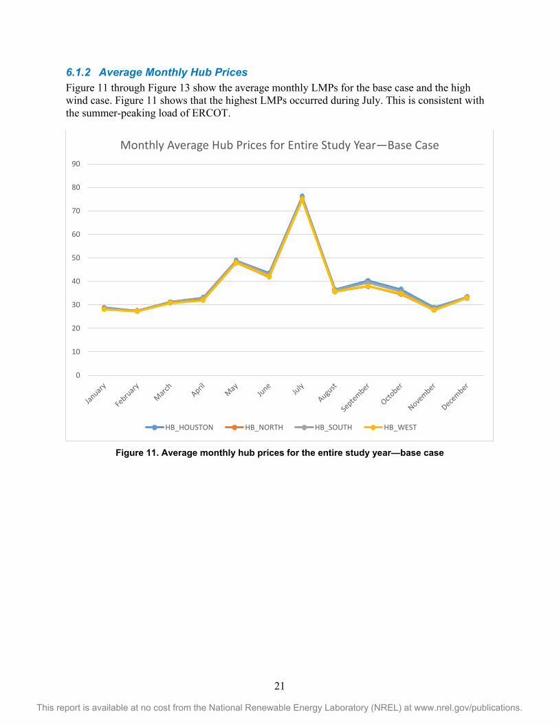
6.1.2 Average Monthly Hub Prices Figure 11 through Figure 13 show the average monthly LMPs for the base case and the high wind case. Figure 11 shows that the highest LMPs occurred during July. This is consistent with the summer-peaking load of ERCOT.

Figure 11. Average monthly hub prices for the entire study year—base case

0

10

20

30

40

50

60

70

80

90

Monthly Average Hub Prices for Entire Study Year—Base Case


22


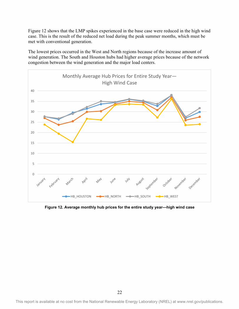
Figure 12 shows that the LMP spikes experienced in the base case were reduced in the high wind case. This is the result of the reduced net load during the peak summer months, which must be met with conventional generation.

The lowest prices occurred in the West and North regions because of the increase amount of wind generation. The South and Houston hubs had higher average prices because of the network congestion between the wind generation and the major load centers.

Figure 12. Average monthly hub prices for the entire study year—high wind case

0

5

10

15

20

25

30

35

40

Monthly Average Hub Prices for Entire Study Year— High Wind Case


23


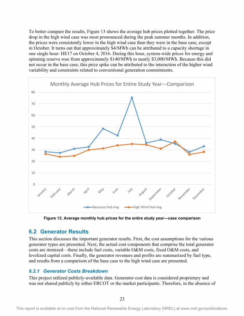
To better compare the results, Figure 13 shows the average hub prices plotted together. The price drop in the high wind case was most pronounced during the peak summer months. In addition, the prices were consistently lower in the high wind case than they were in the base case, except in October. It turns out that approximately $4/MWh can be attributed to a capacity shortage in one single hour: HE17 on October 4, 2016. During this hour, system-wide prices for energy and spinning reserve rose from approximately $140/MWh to nearly $3,000/MWh. Because this did not occur in the base case, this price spike can be attributed to the interaction of the higher wind variability and constraints related to conventional generation commitments.

Figure 13. Average monthly hub prices for the entire study year—case comparison

6.2 Generator Results This section discusses the important generator results. First, the cost assumptions for the various generator types are presented. Next, the actual cost components that comprise the total generator costs are itemized—these include fuel costs, variable O&M costs, fixed O&M costs, and levelized capital costs. Finally, the generator revenues and profits are summarized by fuel type, and results from a comparison of the base case to the high wind case are presented.

6.2.1 Generator Costs Breakdown This project utilized publicly-available data. Generator cost data is considered proprietary and was not shared publicly by either ERCOT or the market participants. Therefore, in the absence of

0

10

20

30

40

50

60

70

80

Monthly Average Hub Prices for Entire Study Year—Comparison

Basecase Hub Avg High Wind Hub Avg

24


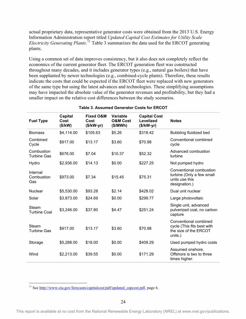
actual proprietary data, representative generator costs were obtained from the 2013 U.S. Energy Information Administration report titled Updated Capital Cost Estimates for Utility Scale Electricity Generating Plants.11 Table 3 summarizes the data used for the ERCOT generating plants.

Using a common set of data improves consistency, but it also does not completely reflect the economics of the current generator fleet. The ERCOT generation fleet was constructed throughout many decades, and it includes generator types (e.g., natural gas boilers) that have been supplanted by newer technologies (e.g., combined-cycle plants). Therefore, these results indicate the costs that could be expected if the ERCOT fleet were replaced with new generators of the same type but using the latest advances and technologies. These simplifying assumptions may have impacted the absolute value of the generator revenues and profitability, but they had a smaller impact on the relative cost differences between the study scenarios.

Table 3. Assumed Generator Costs for ERCOT

Fuel Type Capital Cost ($/kW)

Fixed O&M Cost ($/kW-yr)

Variable O&M Cost ($/MWh)

Capital Cost Levelized ($/kW-yr)

Notes

Biomass $4,114.00 $105.63 $5.26 $318.42 Bubbling fluidized bed

Combined Cycle $917.00 $13.17 $3.60 $70.98 Conventional combined

cycle

Combustion Turbine Gas $676.00 $7.04 $10.37 $52.32 Advanced combustion

turbine

Hydro $2,936.00 $14.13 $0.00 $227.25 Not pumped hydro


$973.00 $7.34 $15.45 $75.31

Conventional combustion turbine (Only a few small units use this designation.)

Nuclear $5,530.00 $93.28 $2.14 $428.02 Dual unit nuclear

Solar $3,873.00 $24.69 $0.00 $299.77 Large photovoltaic

Steam Turbine Coal $3,246.00 $37.80 $4.47 $251.24

Single unit, advanced pulverized coal, no carbon capture

Steam Turbine Gas $917.00 $13.17 $3.60 $70.98

Conventional combined cycle (This fits best with the size of the ERCOT units.)

Storage $5,288.00 $18.00 $0.00 $409.29 Used pumped hydro costs

Wind $2,213.00 $39.55 $0.00 $171.29 Assumed onshore. Offshore is two to three times higher.

11 See http://www.eia.gov/forecasts/capitalcost/pdf/updated_capcost.pdf, page 6.

http://www.eia.gov/forecasts/capitalcost/pdf/updated_capcost.pdf

25


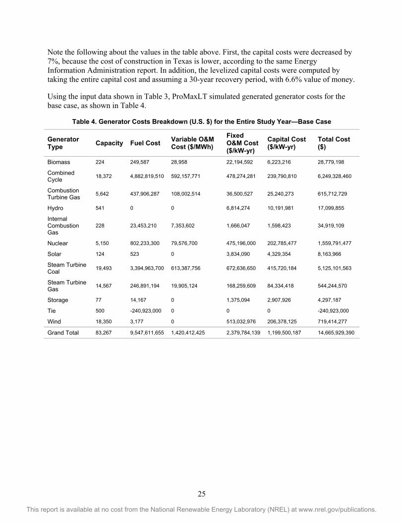
Note the following about the values in the table above. First, the capital costs were decreased by 7%, because the cost of construction in Texas is lower, according to the same Energy Information Administration report. In addition, the levelized capital costs were computed by taking the entire capital cost and assuming a 30-year recovery period, with 6.6% value of money.

Using the input data shown in Table 3, ProMaxLT simulated generated generator costs for the base case, as shown in Table 4.

Table 4. Generator Costs Breakdown (U.S. $) for the Entire Study Year—Base Case

Generator Type Capacity Fuel Cost Variable O&M

Cost ($/MWh) Fixed O&M Cost ($/kW-yr)

Capital Cost ($/kW-yr)

Total Cost ($)

Biomass 224 249,587 28,958 22,194,592 6,223,216 28,779,198

Combined Cycle 18,372 4,882,819,510 592,157,771 478,274,281 239,790,810 6,249,328,460

Combustion Turbine Gas 5,642 437,906,287 108,002,514 36,500,527 25,240,273 615,712,729

Hydro 541 0 0 6,814,274 10,191,981 17,099,855


228 23,453,210 7,353,602 1,666,047 1,598,423 34,919,109

Nuclear 5,150 802,233,300 79,576,700 475,196,000 202,785,477 1,559,791,477

Solar 124 523 0 3,834,090 4,329,354 8,163,966

Steam Turbine Coal 19,493 3,394,963,700 613,387,756 672,636,650 415,720,184 5,125,101,563

Steam Turbine Gas 14,567 246,891,194 19,905,124 168,259,609 84,334,418 544,244,570

Storage 77 14,167 0 1,375,094 2,907,926 4,297,187

Tie 500 -240,923,000 0 0 0 -240,923,000

Wind 18,350 3,177 0 513,032,976 206,378,125 719,414,277

Grand Total 83,267 9,547,611,655 1,420,412,425 2,379,784,139 1,199,500,187 14,665,929,390

26


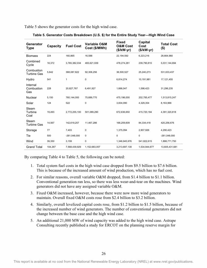
Table 5 shows the generator costs for the high wind case.

Table 5. Generator Costs Breakdown (U.S. $) for the Entire Study Year—High Wind Case

Generator Type Capacity Fuel Cost Variable O&M

Cost ($/MWh) Fixed O&M Cost ($/kW-yr)

Capital Cost ($/kW-yr)

Total Cost ($)

Biomass 224 160,865 16,588 22,194,592 6,223,216 28,664,980

Combined Cycle 18,372 3,765,382,034 465,621,939 478,274,281 239,790,810 5,031,144,694

Combustion Turbine Gas 5,642 368,087,822 92,306,256 36,500,527 25,240,273 531,633,437

Hydro 541 1 0 6,814,274 10,191,981 17,121,455


228 20,827,767 6,491,927 1,666,047 1,598,423 31,296,235

Nuclear 5,150 760,144,000 75,689,770 475,196,000 202,785,477 1,513,815,247

Solar 124 522 0 3,834,090 4,329,354 8,163,966

Steam Turbine Coal

19,493 2,772,255,100 501,089,290 672,636,650 415,720,184 4,391,320,818

Steam Turbine Gas 14,567 142,619,257 11,467,286 168,259,609 84,334,418 420,256,676

Storage 77 7,403 0 1,375,094 2,907,926 4,290,423

Tie 500 -261,048,000 0 0 0 -261,048,000

Wind 39,350 3,159 0 1,346,945,976 541,822,615 1,888,771,750

Grand Total 104,267 7,568,439,929 1,152,683,057 3,213,697,139 1,534,944,677 13,605,431,681

By comparing Table 4 to Table 5, the following can be noted:

1. Total system fuel costs in the high wind case dropped from $9.5 billion to $7.6 billion. This is because of the increased amount of wind production, which has no fuel cost.

2. For similar reasons, overall variable O&M dropped, from $1.4 billion to $1.1 billion. Conventional generation ran less, so there was less wear-and-tear on the machines. Wind generators did not have any assigned variable O&M.

3. Fixed O&M increased, however, because there were now more wind generators to maintain. Overall fixed O&M costs rose from $2.4 billion to $3.2 billion.

4. Similarly, overall levelized capital costs rose, from $1.2 billion to $1.5 billion, because of the increased number of wind generators. The number of conventional generators did not change between the base case and the high wind case.

5. An additional 21,000 MW of wind capacity was added to the high wind case. Astrape Consulting recently published a study for ERCOT on the planning reserve margin for

27


2016.12 They determined a wind capacity factor of 56% for coastal wind and 12% for non-coastal wind. Given that this study used non-coastal wind, it would have a capacity value of 12% * 21,000 = 2,520 MW, based on the current ERCOT planning parameters.

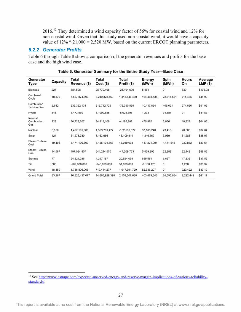
6.2.2 Generator Profits Table 6 through Table 8 show a comparison of the generator revenues and profits for the base case and the high wind case.

Table 6. Generator Summary for the Entire Study Year—Base Case

Generator Type Capacity Total

Revenue ($) Total Cost ($)

Total Profit ($)

Energy (MWh)

Spin (MWh)

Hours On

Average LMP ($)

Biomass 224 584,508 28,779,198 -28,194,690 5,464 0 639 $106.98

Combined Cycle 18,372 7,567,874,890 6,249,328,460 1,318,546,430 164,488,135 22,614,561 714,485 $44.90

Combustion Turbine Gas 5,642 539,362,134 615,712,729 -76,350,595 10,417,864 405,021 274,836 $51.03

Hydro 541 8,473,960 17,099,855 -8,625,895 1,293 34,587 91 $41.57


228 30,723,207 34,919,109 -4,195,902 475,970 3,866 10,829 $64.05

Nuclear 5,150 1,407,191,900 1,559,791,477 -152,599,577 37,185,240 23,410 28,500 $37.84

Solar 124 51,273,780 8,163,966 43,109,814 1,346,562 3,069 61,283 $38.07

Steam Turbine Coal 19,493 5,171,190,600 5,125,101,563 46,089,038 137,221,991 1,471,643 230,852 $37.61

Steam Turbine Gas 14,567 497,034,807 544,244,570 -47,209,763 5,529,206 32,288 22,449 $88.82

Storage 77 24,821,286 4,297,187 20,524,099 659,584 6,637 17,833 $37.59

Tie 500 -209,900,000 -240,923,000 31,023,000 -6,188,170 0 1,230 $33.92

Wind 18,350 1,736,806,006 719,414,277 1,017,391,729 52,336,207 0 929,422 $33.19

Grand Total 83,267 16,825,437,077 14,665,929,390 2,159,507,688 403,479,346 24,595,084 2,292,449 $41.17

12 See http://www.astrape.com/expected-unserved-energy-and-reserve-margin-implications-of-various-reliability-standards/.

http://www.astrape.com/expected-unserved-energy-and-reserve-margin-implications-of-various-reliability-standards/

http://www.astrape.com/expected-unserved-energy-and-reserve-margin-implications-of-various-reliability-standards/

28


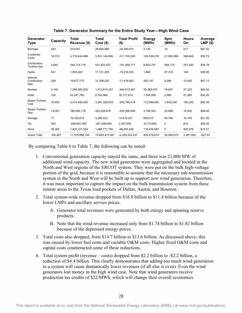
Table 7. Generator Summary for the Entire Study Year—High Wind Case

Generator Type Capacity Total

Revenue ($) Total Cost ($)

Total Profit ($)

Energy (MWh)

Spin (MWh)

Hours On

Average LMP ($)

Biomass 224 274,007 28,664,980 -28,390,974 3,130 14 617 $87.50

Combined Cycle 18,372 4,719,444,468 5,031,144,694 -311,700,226 129,339,276 21,855,066 599,648 $35.79

Combustion Turbine Gas 5,642 349,774,719 531,633,437 -181,858,717 8,903,791 648,174 257,483 $38.79

Hydro 541 1,903,422 17,121,455 -15,218,033 1,883 87,316 146 $39.85


228 19,877,772 31,296,235 -11,418,463 420,197 9,284 10,455 $47.13

Nuclear 5,150 1,059,305,200 1,513,815,247 -454,510,047 35,369,070 78,607 27,323 $29.94

Solar 124 43,341,780 8,163,966 35,177,814 1,345,456 2,985 61,260 $32.20

Steam Turbine Coal 19,493 3,414,555,400 4,391,320,818 -976,765,418 112,099,560 1,832,034 193,202 $30.39

Steam Turbine Gas 14,567 186,890,178 420,256,676 -233,366,499 3,185,353 20,889 14,422 $58.46

Storage 77 19,100,674 4,290,423 14,810,251 606,012 60,706 16,145 $31.06

Tie 500 -258,691,000 -261,048,000 2,357,000 -6,710,640 0 814 $38.55

Wind 39,350 1,820,121,524 1,888,771,750 -68,650,226 118,916,587 0 905,978 $15.31

Grand Total 104,267 11,375,898,144 13,605,431,681 -2,229,533,537 403,479,674 24,595,075 2,087,493 $27.93

By comparing Table 6 to Table 7, the following can be noted:

1. Conventional generation capacity stayed the same, and there was 21,000 MW of additional wind capacity. The new wind generators were aggregated and located in the North and West regions of the ERCOT system. They were put on the bulk high-voltage portion of the grid, because it is reasonable to assume that the necessary sub-transmission system in the North and West will be built up to support new wind generation. Therefore, it was most important to capture the impact on the bulk transmission system from these remote areas to the Texas load pockets of Dallas, Austin, and Houston.

2. Total system-wide revenue dropped from $16.8 billion to $11.4 billion because of the lower LMPs and ancillary service prices.

A. Generator total revenues were generated by both energy and spinning reserve products.

B. Note that the wind revenue increased only from $1.74 billion to $1.82 billion because of the depressed energy prices.

3. Total costs also dropped, from $14.7 billion to $13.6 billion. As discussed above, this was caused by lower fuel costs and variable O&M costs. Higher fixed O&M costs and capital costs counteracted some of these reductions.

4. Total system profit (revenue – costs) dropped from $2.2 billion to -$2.2 billion, a reduction of $4.4 billion. This clearly demonstrates that adding too much wind generation to a system will cause dramatically lower revenues (if all else is even). Even the wind generators lost money in the high wind case. Note that wind generators receive production tax credits of $22/MWh, which will change their overall economics.

29


5. Total wind production increased from 52 TWh to 119 TWh. Note that this is the amount of delivered wind energy, because a non-trivial amount of wind was curtailed by the system. The exact wind curtailment is presented in Section 6.3.

6. Average generator LMP dropped from $41.17 in the base case to $27.93 in the high wind case. This drove lower generator revenues, which then resulted in reduced profitability for the generator fleet.

7. The magnitude of the generator revenues and profits depends on the market structure. The prevailing market design is based on the marginal costs of production, and therefore they will be significantly impacted by the addition of resources that do not have incremental fuel costs.

8. Note that conventional generation capacity in the high wind case was not adjusted. Economic theory is clear that the addition of generating capacity (wind or conventional) will lower prices and revenues. Further studies could examine the impact of a more optimal generation fleet, in which excess generating capacity would be minimized.

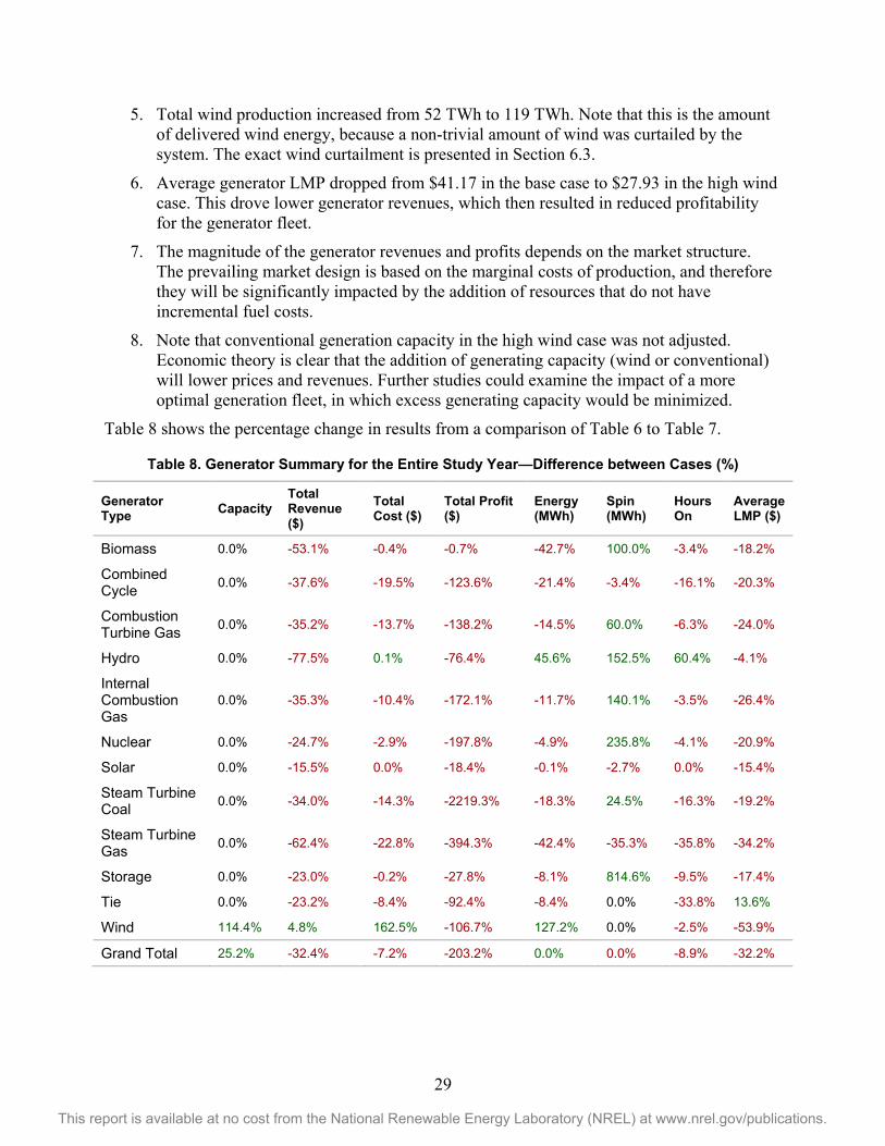
Table 8 shows the percentage change in results from a comparison of Table 6 to Table 7.

Table 8. Generator Summary for the Entire Study Year—Difference between Cases (%)

Generator Type Capacity

Total Revenue ($)

Total Cost ($)

Total Profit ($)

Energy (MWh)

Spin (MWh)

Hours On

Average LMP ($)

Biomass 0.0% -53.1% -0.4% -0.7% -42.7% 100.0% -3.4% -18.2%

Combined Cycle 0.0% -37.6% -19.5% -123.6% -21.4% -3.4% -16.1% -20.3%

Combustion Turbine Gas 0.0% -35.2% -13.7% -138.2% -14.5% 60.0% -6.3% -24.0%

Hydro 0.0% -77.5% 0.1% -76.4% 45.6% 152.5% 60.4% -4.1%


0.0% -35.3% -10.4% -172.1% -11.7% 140.1% -3.5% -26.4%

Nuclear 0.0% -24.7% -2.9% -197.8% -4.9% 235.8% -4.1% -20.9%

Solar 0.0% -15.5% 0.0% -18.4% -0.1% -2.7% 0.0% -15.4%

Steam Turbine Coal 0.0% -34.0% -14.3% -2219.3% -18.3% 24.5% -16.3% -19.2%

Steam Turbine Gas 0.0% -62.4% -22.8% -394.3% -42.4% -35.3% -35.8% -34.2%

Storage 0.0% -23.0% -0.2% -27.8% -8.1% 814.6% -9.5% -17.4%

Tie 0.0% -23.2% -8.4% -92.4% -8.4% 0.0% -33.8% 13.6%

Wind 114.4% 4.8% 162.5% -106.7% 127.2% 0.0% -2.5% -53.9%

Grand Total 25.2% -32.4% -7.2% -203.2% 0.0% 0.0% -8.9% -32.2%

30


Red values indicate a drop in the results from the high wind case, whereas green values indicate an increase in the results from the high wind case. Note the following:

1. Conventional (nuclear, coal, gas) generation was most negatively impacted, including in the areas of energy production, hours on, total revenue, and total profit.

2. Conventional generators cleared more spinning reserve, but this is because they were producing less energy and had more unloaded capacity. However, this additional of available spinning reserve caused the average spin price to drop from $8.71/MWh in the base case to $4.33/MWh in the high wind case (not shown in table). This is consistent with the basic market fundamentals that prices drop when supplies increase, and demand remained constant. Therefore, conventional generators produced less energy and faced lower spinning reserve prices because of the system surplus of spin capacity.

3. Hydro showed a modest increase in production (45.6%), but hydro is a very small player in ERCOT. In the studies, hydro averaged less than 1MW production each hour, although it did provide some additional spinning reserve.

4. Wind production was up 127.2%, but wind revenue increased only 4.8%. With the additional wind generator costs, this resulted in a market loss (negative profit) for the wind generators. Wind generators also have non-market revenue streams, however, which would likely make them profitable. For example, since 1992 there has been a federal production tax credit of $22/MWh for wind generation.

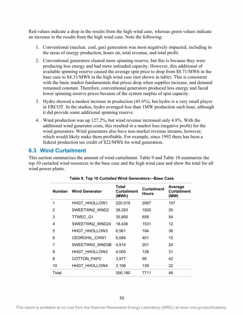
6.3 Wind Curtailment This section summarizes the amount of wind curtailment. Table 9 and Table 10 summarize the top 10 curtailed wind resources in the base case and the high wind case and show the total for all wind power plants.

Table 9. Top 10 Curtailed Wind Generators—Base Case

Number Wind Generator Total Curtailment (MWh)

Curtailment Hours

Average Curtailment (MW)

1 HHGT_HHOLLOW1 220,519 2067 107

2 SWEETWN2_WND2 39,293 1920 20

3 TTWEC_G1 35,850 658 54

4 SWEETWN2_WND24 18,436 1531 12

5 HHGT_HHOLLOW3 6,561 184 36

6 CEDROHIL_CHW1 6,084 401 15

7 SWEETWN3_WND3B 4,914 201 24

8 HHGT_HHOLLOW2 4,005 128 31

9 COTTON_PAP2 3,977 95 42

10 HHGT_HHOLLOW4 3,106 139 22

Total 356,180 7711 46

31


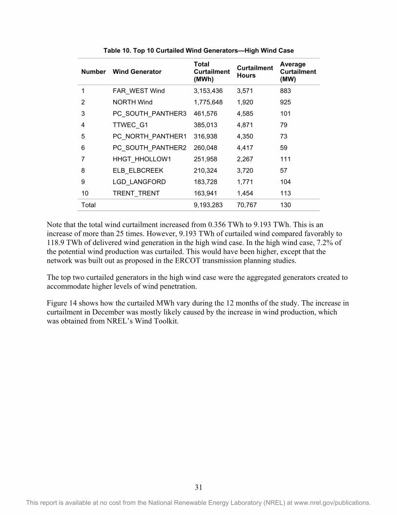
Table 10. Top 10 Curtailed Wind Generators—High Wind Case

Number Wind Generator Total Curtailment (MWh)

Curtailment Hours

Average Curtailment (MW)

1 FAR_WEST Wind 3,153,436 3,571 883

2 NORTH Wind 1,775,648 1,920 925

3 PC_SOUTH_PANTHER3 461,576 4,585 101

4 TTWEC_G1 385,013 4,871 79

5 PC_NORTH_PANTHER1 316,938 4,350 73

6 PC_SOUTH_PANTHER2 260,048 4,417 59

7 HHGT_HHOLLOW1 251,958 2,267 111

8 ELB_ELBCREEK 210,324 3,720 57

9 LGD_LANGFORD 183,728 1,771 104

10 TRENT_TRENT 163,941 1,454 113

Total 9,193,283 70,767 130

Note that the total wind curtailment increased from 0.356 TWh to 9.193 TWh. This is an increase of more than 25 times. However, 9.193 TWh of curtailed wind compared favorably to 118.9 TWh of delivered wind generation in the high wind case. In the high wind case, 7.2% of the potential wind production was curtailed. This would have been higher, except that the network was built out as proposed in the ERCOT transmission planning studies.

The top two curtailed generators in the high wind case were the aggregated generators created to accommodate higher levels of wind penetration.

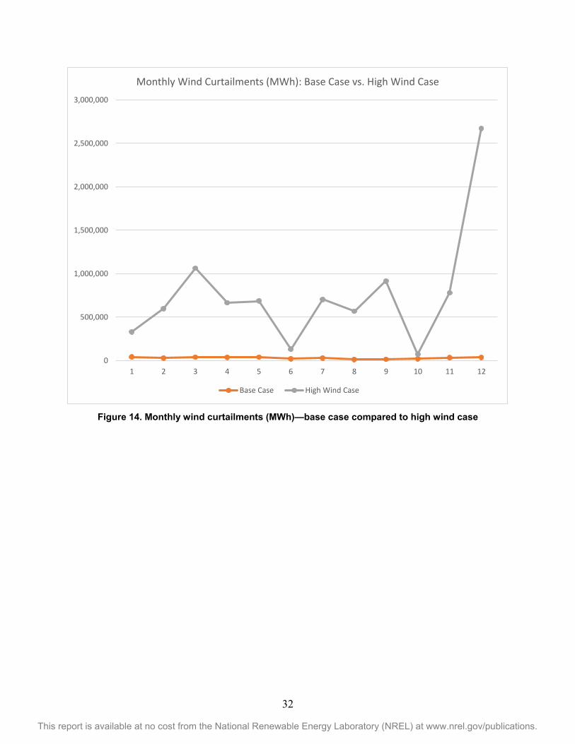
Figure 14 shows how the curtailed MWh vary during the 12 months of the study. The increase in curtailment in December was mostly likely caused by the increase in wind production, which was obtained from NREL’s Wind Toolkit.

32


Figure 14. Monthly wind curtailments (MWh)—base case compared to high wind case

0

500,000

1,000,000

1,500,000

2,000,000

2,500,000

3,000,000

1 2 3 4 5 6 7 8 9 10 11 12

Monthly Wind Curtailments (MWh): Base Case vs. High Wind Case

Base Case High Wind Case

33


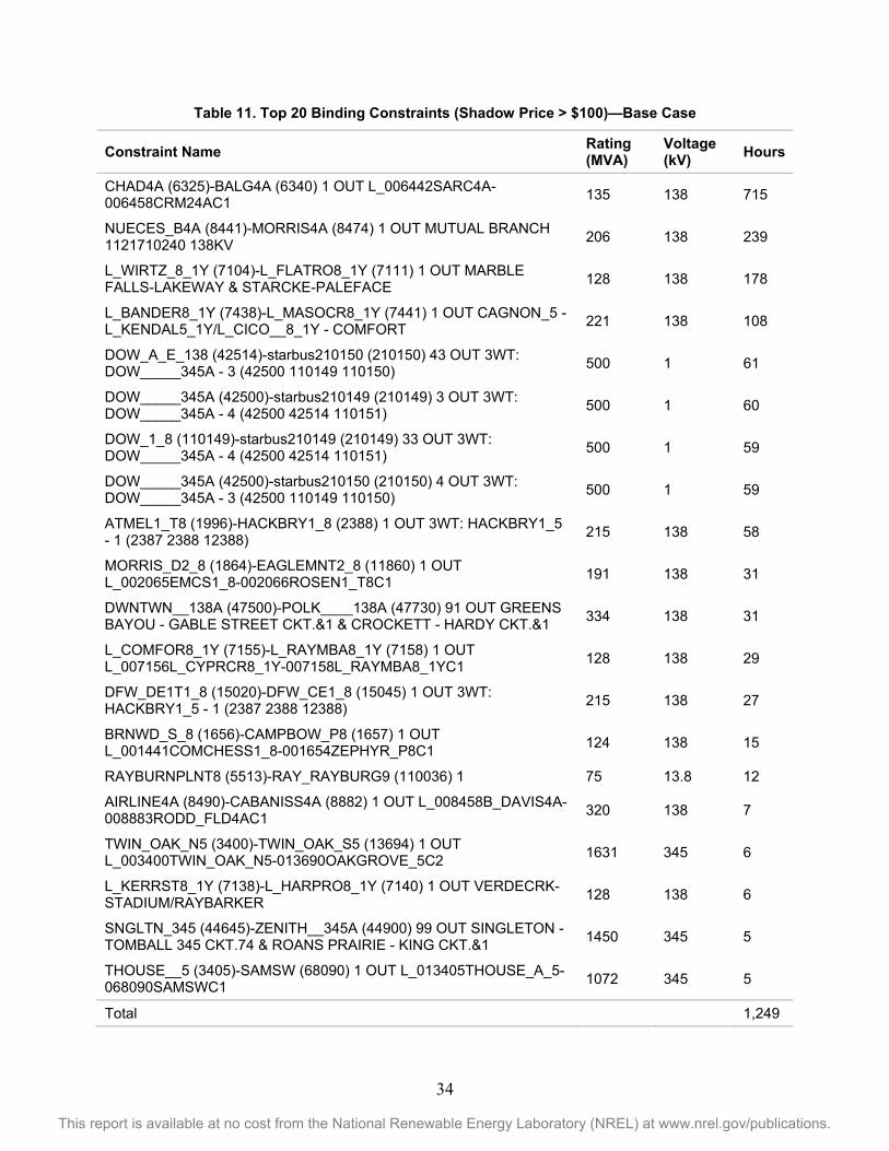
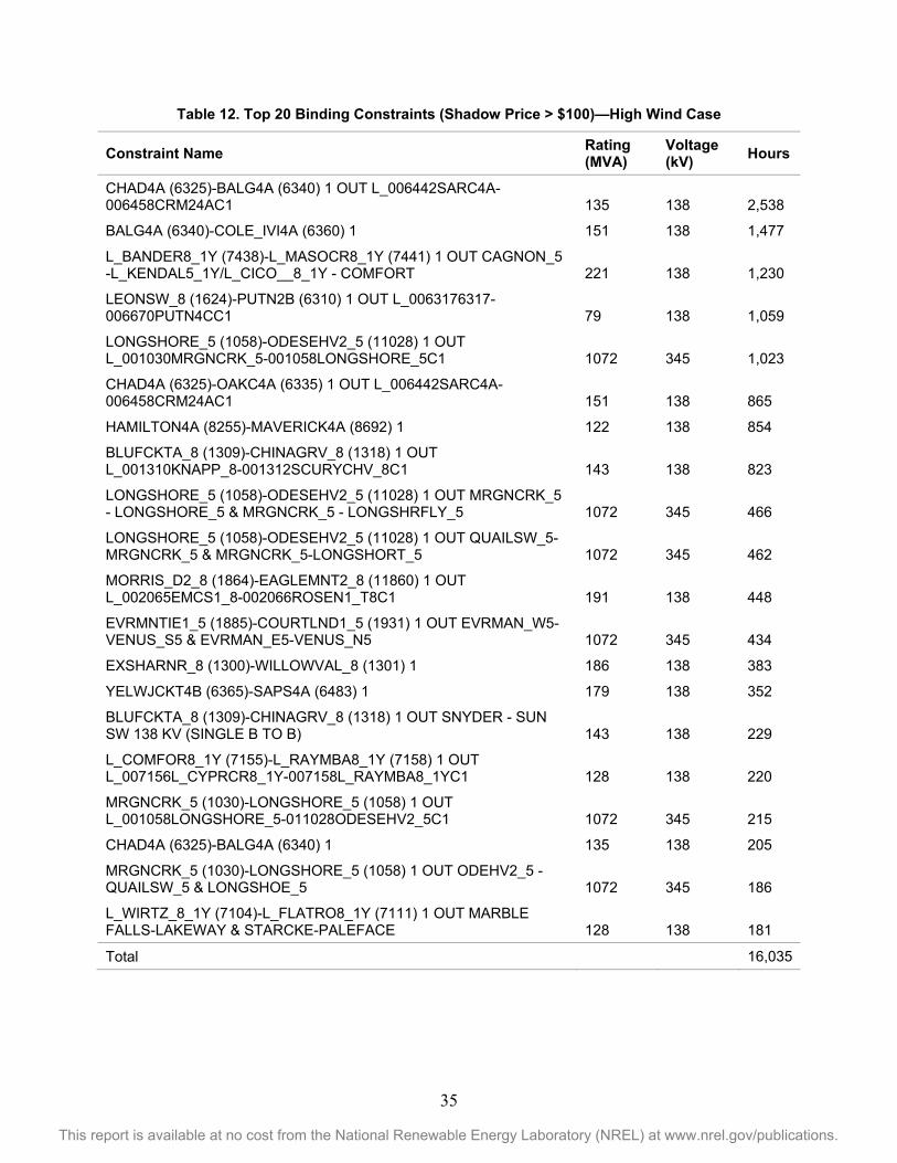
7 Binding Constraints This study deployed a full and detailed network model that allowed the results to capture the impacts of the transmission constraints. As described above in Section 3.2, the network model was augmented with additional lines per the ERCOT planning study.

Table 11 and Table 12 summarize the top 20 binding constraints in the base case and the high wind case. To capture only strongly binding constraints, a shadow price (dual) cutoff of $100/MW was enforced.

34


Table 11. Top 20 Binding Constraints (Shadow Price > $100)—Base Case

Constraint Name Rating (MVA)

Voltage (kV) Hours

CHAD4A (6325)-BALG4A (6340) 1 OUT L_006442SARC4A-006458CRM24AC1 135 138 715

NUECES_B4A (8441)-MORRIS4A (8474) 1 OUT MUTUAL BRANCH 1121710240 138KV 206 138 239

L_WIRTZ_8_1Y (7104)-L_FLATRO8_1Y (7111) 1 OUT MARBLE FALLS-LAKEWAY & STARCKE-PALEFACE 128 138 178

L_BANDER8_1Y (7438)-L_MASOCR8_1Y (7441) 1 OUT CAGNON_5 -L_KENDAL5_1Y/L_CICO__8_1Y - COMFORT 221 138 108

DOW_A_E_138 (42514)-starbus210150 (210150) 43 OUT 3WT: DOW_____345A - 3 (42500 110149 110150) 500 1 61

DOW_____345A (42500)-starbus210149 (210149) 3 OUT 3WT: DOW_____345A - 4 (42500 42514 110151) 500 1 60

DOW_1_8 (110149)-starbus210149 (210149) 33 OUT 3WT: DOW_____345A - 4 (42500 42514 110151) 500 1 59

DOW_____345A (42500)-starbus210150 (210150) 4 OUT 3WT: DOW_____345A - 3 (42500 110149 110150) 500 1 59

ATMEL1_T8 (1996)-HACKBRY1_8 (2388) 1 OUT 3WT: HACKBRY1_5 - 1 (2387 2388 12388) 215 138 58

MORRIS_D2_8 (1864)-EAGLEMNT2_8 (11860) 1 OUT L_002065EMCS1_8-002066ROSEN1_T8C1 191 138 31

DWNTWN__138A (47500)-POLK____138A (47730) 91 OUT GREENS BAYOU - GABLE STREET CKT.&1 & CROCKETT - HARDY CKT.&1 334 138 31

L_COMFOR8_1Y (7155)-L_RAYMBA8_1Y (7158) 1 OUT L_007156L_CYPRCR8_1Y-007158L_RAYMBA8_1YC1 128 138 29

DFW_DE1T1_8 (15020)-DFW_CE1_8 (15045) 1 OUT 3WT: HACKBRY1_5 - 1 (2387 2388 12388) 215 138 27

BRNWD_S_8 (1656)-CAMPBOW_P8 (1657) 1 OUT L_001441COMCHESS1_8-001654ZEPHYR_P8C1 124 138 15

RAYBURNPLNT8 (5513)-RAY_RAYBURG9 (110036) 1 75 13.8 12

AIRLINE4A (8490)-CABANISS4A (8882) 1 OUT L_008458B_DAVIS4A-008883RODD_FLD4AC1 320 138 7

TWIN_OAK_N5 (3400)-TWIN_OAK_S5 (13694) 1 OUT L_003400TWIN_OAK_N5-013690OAKGROVE_5C2 1631 345 6

L_KERRST8_1Y (7138)-L_HARPRO8_1Y (7140) 1 OUT VERDECRK-STADIUM/RAYBARKER 128 138 6

SNGLTN_345 (44645)-ZENITH__345A (44900) 99 OUT SINGLETON - TOMBALL 345 CKT.74 & ROANS PRAIRIE - KING CKT.&1 1450 345 5

THOUSE__5 (3405)-SAMSW (68090) 1 OUT L_013405THOUSE_A_5-068090SAMSWC1 1072 345 5

Total 1,249

35


Table 12. Top 20 Binding Constraints (Shadow Price > $100)—High Wind Case

Constraint Name Rating (MVA)

Voltage (kV) Hours

CHAD4A (6325)-BALG4A (6340) 1 OUT L_006442SARC4A-006458CRM24AC1 135 138 2,538

BALG4A (6340)-COLE_IVI4A (6360) 1 151 138 1,477

L_BANDER8_1Y (7438)-L_MASOCR8_1Y (7441) 1 OUT CAGNON_5 -L_KENDAL5_1Y/L_CICO__8_1Y - COMFORT 221 138 1,230

LEONSW_8 (1624)-PUTN2B (6310) 1 OUT L_0063176317-006670PUTN4CC1 79 138 1,059

LONGSHORE_5 (1058)-ODESEHV2_5 (11028) 1 OUT L_001030MRGNCRK_5-001058LONGSHORE_5C1 1072 345 1,023

CHAD4A (6325)-OAKC4A (6335) 1 OUT L_006442SARC4A-006458CRM24AC1 151 138 865

HAMILTON4A (8255)-MAVERICK4A (8692) 1 122 138 854

BLUFCKTA_8 (1309)-CHINAGRV_8 (1318) 1 OUT L_001310KNAPP_8-001312SCURYCHV_8C1 143 138 823

LONGSHORE_5 (1058)-ODESEHV2_5 (11028) 1 OUT MRGNCRK_5 - LONGSHORE_5 & MRGNCRK_5 - LONGSHRFLY_5 1072 345 466

LONGSHORE_5 (1058)-ODESEHV2_5 (11028) 1 OUT QUAILSW_5-MRGNCRK_5 & MRGNCRK_5-LONGSHORT_5 1072 345 462

MORRIS_D2_8 (1864)-EAGLEMNT2_8 (11860) 1 OUT L_002065EMCS1_8-002066ROSEN1_T8C1 191 138 448

EVRMNTIE1_5 (1885)-COURTLND1_5 (1931) 1 OUT EVRMAN_W5-VENUS_S5 & EVRMAN_E5-VENUS_N5 1072 345 434

EXSHARNR_8 (1300)-WILLOWVAL_8 (1301) 1 186 138 383

YELWJCKT4B (6365)-SAPS4A (6483) 1 179 138 352

BLUFCKTA_8 (1309)-CHINAGRV_8 (1318) 1 OUT SNYDER - SUN SW 138 KV (SINGLE B TO B) 143 138 229

L_COMFOR8_1Y (7155)-L_RAYMBA8_1Y (7158) 1 OUT L_007156L_CYPRCR8_1Y-007158L_RAYMBA8_1YC1 128 138 220

MRGNCRK_5 (1030)-LONGSHORE_5 (1058) 1 OUT L_001058LONGSHORE_5-011028ODESEHV2_5C1 1072 345 215

CHAD4A (6325)-BALG4A (6340) 1 135 138 205

MRGNCRK_5 (1030)-LONGSHORE_5 (1058) 1 OUT ODEHV2_5 - QUAILSW_5 & LONGSHOE_5 1072 345 186

L_WIRTZ_8_1Y (7104)-L_FLATRO8_1Y (7111) 1 OUT MARBLE FALLS-LAKEWAY & STARCKE-PALEFACE 128 138 181

Total 16,035

36


Because of the higher amount of wind generation in remote locations, more congestion was experienced in the high wind case. Overall, the number of binding constraints with a shadow price > $100 increased from 1,249 constraint hours to 16,035 constraint hours.

The dominant constraint in both cases was the post-contingent constraint CHAD4A (6325)-BALG4A (6340) 1 OUT L_006442SARC4A-006458CRM24AC1. In the base case, it bound in 715 hours. In the high wind case, it bound in 2,538 hours.

At a high-level, the impact of the transmission system had the expected impact on the simulation results.

• In the base case, congestion was minimal (Table 11). Hub prices were nearly identical, which indicates that there was very little intra-zonal congestion (Figure 8).

• In the high wind case, there was significantly more congestion (Table 12).

• There was a differential in the hub prices (Figure 9). The lower prices were experienced in the North and West hubs, which is where the new wind generation was sited.

• The amount of curtailment was 7.2% of the total potential wind production (high wind case), which indicates that there was congestion between the wind generation and the main load regions, but also that it was not overly excessive at this wind penetration level.

• The observed levels of congestion and curtailment in the high wind case in this study are plausible, and they should not have an unreasonable impact on the missing money problem. If all congestion and curtailment were eliminated, this would add (on average) slightly more than 1,000 MW of wind generation each hour. This would incrementally depress the average prices, revenues, and profits, but it would not materially change the primary findings.

37


8 Conclusion This project examined the impact of renewable energy sources, which have zero incremental energy costs, on the sustainability of conventional generation. This missing money problem is caused by two related factors: (1) conventional generation is dispatched less, and (2) the prices that conventional forms of generation receive for its energy are lower. This lower revenue stream may not be sufficient to cover both its variable and fixed costs. In fact, this study showed that higher wind penetrations in the ERCOT system could cause many conventional generators to become uneconomic.

For continuity, all generator costs used in this paper were obtained from the 2013 U.S. Energy Information Administration report titled Updated Capital Cost Estimates for Utility Scale Electricity Generating Plants. This ensured that any inconsistencies in the data could be eliminated. Also, the current ERCOT fleet was constructed throughout many decades, which makes it difficult to compare capital costs, and therefore these results indicate the costs that could be expected if the ERCOT fleet were replaced with new generators of the same type but using the latest advances and technologies.

Two cases were examined: (1) the base case, in which 13% of the energy was met with wind; and (2) the high wind case, in which 30% of the energy was met with wind. An additional 2.2% of the load in the high wind case could have been met with wind, but the energy was curtailed because of network congestion.

The ERCOT base case simulation was reasonable based on recent performance. Specifically:

• The average generator LMP was $41.17.

• LMPs increased during peak afternoon hours and during peak summer months.

• With the current network build out, there was little congestion with the current levels of wind production.

The high wind case also resulted in reasonable metrics:

• The average generator LMP dropped to $27.93.

• When compared to the base case, prices were depressed across almost all hours and seasons because of the increased amount of wind generation with no marginal costs.

• Congestion in the network resulted in lower hub prices in the West and North. Load centers in the South and Houston saw relatively higher prices.

Because of the higher amount of wind generation in remote locations, more congestion was experienced in the high wind case. Overall, the number of binding constraints with a shadow price > $100 increased from 1,249 constraint hours in the base case to 16,035 constraint hours in the high wind case.

Generation was impacted by higher wind production in the following ways:

• Conventional (nuclear, coal, gas) generation was most negatively impacted. These units had dramatically reduced energy production, hours on, total revenue, and total profit.

38


o Conventional generation cleared more spinning reserve, but this is because it produced less energy. This was offset, however, by the large spinning reserve ancillary service price drop in the high wind case, from $8.71/MWh to $4.33/MWh.

• Overall system-wide generator fixed costs increased, because additional wind generators were being built and maintained.

o Overall fixed O&M costs rose from $2.4 billion to $3.2 billion. o Similarly, overall levelized capital costs rose from $1.2 billion to $1.5 billion per

year. • Overall system-wide generator variable costs dropped because of the reduced production

from conventional generators. o Total system fuel costs dropped from $9.5 billion to $7.6 billion. o Overall variable O&M costs dropped from $1.4 billion to $1.1 billion.

• The largest impact was on overall system-wide generator revenues and profits o Total system-wide revenue dropped from $16.8 billion to $11.4 billion because of

the lower LMPs and ancillary service prices. o Total system profit (revenue – costs) dropped from $2.2 billion to -$2.2 billion, a

reduction of $4.4 billion. o Wind generator revenue increased marginally, from $1.74 billion to $1.82 billion,

because of the depressed energy prices. With higher fixed costs, even wind generation lost money in the market in the high wind case. Note that wind generators receive non-market production tax credits, which will improve their financial viability.

o The magnitude of the generator revenues and profits depends on the market structure. The prevailing market design is based on the marginal costs of production, and therefore it will be significantly impacted by the addition of resources that do not have incremental fuel costs.

o Note that conventional generation capacity in the high wind case was not adjusted. Economic theory is clear that additional generating capacity (wind or conventional) will lower prices and revenues. Further studies could examine the impact of a more optimal generation fleet, in which excess generating capacity would be minimized.

o The observed levels of congestion and curtailment in the high wind case in this study are plausible and should not have an unreasonable impact on the missing money problem. If all congestion and curtailment were eliminated, this would add (on average) slightly more than 1,000 MW of wind generation each hour. This would incrementally depress the average prices, revenues, and profits, but it would not materially change the primary findings.

This study quantified the impact of increased wind production on conventional generation in the ERCOT system. This missing money in organized electricity markets has the potential to inhibit new construction of conventional generation, which may in turn lead to a less reliable electric power system.

39


References Energy Information Administration. (2013). Updated Capital Cost Estimates for Utility Scale Electricity Generating Plants. Washington, DC.

ERCOT. (2013). Expansion Wind Data Used in LTS. http://www.ercot.com/content/committees/other/lts/keydocs/2013/expansion_wind_unit_data_used_in_LTS.xls.

ERCOT. (2014). Panhandle Renewable Energy Zone (PREZ) Study Report. Austin, TX. http://www.ercot.com/content/news/presentations/2014/Panhandle%20Renewable%20Energy%20Zone%20Study%20Report.pdf.

Vittal. V. (2010). “The Impact of Renewable Resources on the Performance and Reliability of the Electricity Grid.” National Academy of Engineering: The Bridge on the Electricity Grid (40:1); spring.



http://www.ercot.com/content/news/presentations/2014/Panhandle%20Renewable%20Energy%20Zone%20Study%20Report.pdf

http://www.ercot.com/content/news/presentations/2014/Panhandle%20Renewable%20Energy%20Zone%20Study%20Report.pdf

Understanding the Missing Money Problem

Documents

Transcript of Understanding the Missing Money Problem