DOCUMENTO DE TRABAJO

UNDERSTANDING THEEFFECTS OF GOVERNMENT

SPENDING ONCONSUMPTION

Documento de Trabajo n.º 0321

BANCO DE ESPAÑA

SERVICIO DE ESTUDIOS

and Javier VallésJordi Galí, J. David López Salido

UNDERSTANDING THE EFFECTS OF GOVERNMENT

SPENDING ON CONSUMPTION (*)

Documento de Trabajo nº 0321

Jordi Galí CREI AND UNIVERSITAT POMPEU FABRA

J. David López Salido BANCO DE ESPAÑA

Javier VallésBANCO DE ESPAÑA

(*) We wish to thank Alberto Alesina, Javier Andrés, Gabriel Fagan, Eric Leeper, Ilian Mihov, Roberto Perotti, Valery Ramey, Jaume Ventura, an annonymous referee and seminar participants at the Bank of Spain, Bank of England, CREI-UPF, IGIER-Bocconi, INSEAD, York, Salamanca, NBER Summer Institute 2002, the 1st Workshop on Dynamic Macroeconomics at Hydra, the EEA Meetings in Stockholmand the 2nd International Research Forum on Monetary Policy for useful comments and suggestions. Galí acknowledges the financial support and hospitality of the Banco de España.

BANCO DE ESPAÑA SERVICIO DE ESTUDIOS

The Working Paper Series seeks to disseminate original research in economics and finance. All papers have been anonymously refereed. By publishing these papers, the Banco de España

aims to contribute to economic analysis and, in particular, to knowledge of the Spanish economy and its international environment.

The opinions and analyses in the Working Paper Series are the responsibility of the authors and,

therefore, do not necessarily coincide with those of the Banco de España or the Eurosystem.

The Banco de España disseminates its main reports and most of its publications via the INTERNET at the following

website: http://www.bde.es

Reproduction for educational and non-commercial purposes is permitted provided that the source is acknowledged

© BANCO DE ESPAÑA, Madrid, 2003 ISSN: 0213-2710 (print)

ISSN: 1579-8666 (online) Depósito legal: M. 5309-2004Imprenta del Banco de España

AbstractRecent evidence on the e¤ect of government spending shocks on consump-

tion cannot be easily reconciled with existing optimizing business cycle models.We extend the standard New Keynesian model to allow for the presence ofrule-of-thumb (non-Ricardian) consumers. We show how the interaction ofthe latter with sticky prices and de…cit …nancing can account for the existingevidence on the e¤ects of government spending.

JEL Classi…cation : E32, E62Keywords: rule-of-thumb consumers, …scal multiplier, government spend-

ing, Taylor rules

1 Introduction

What are the e ects of changes in government purchases of goods and services (hence-

forth, government spending, for short) on aggregate economic activity? How are those

e ects transmitted? Even though such questions are central to macroeconomics and

its ability to inform economic policy, there is no widespread agreement on their an-

swer, either at the empirical or at the theoretical levels.

In particular, though most macroeconomic models predict that a rise in govern-

ment spending will have an expansionary e ect on output, those models often di er

regarding the implied e ects of such a policy intervention on consumption. Since the

latter variable is the largest component of aggregate demand, its response is a key

determinant of the size of the government spending multiplier. In that regard, the

textbook IS-LM model and the standard RBC model provide a stark example of such

di erential qualitative predictions.

Thus, while the standard RBC model generally predicts a decline in consumption

in response to a rise in government spending, the IS-LM model predicts an increase

in the same variable, hence amplifying the e ects of the expansion in government

spending on output. Of course, the reason for the di erential impact across those

two models lies in how consumers are assumed to behave in each case. The RBC

model features an in…nitely-lived household, whose consumption decisions at any

point in time are based on an intertemporal budget contraint. Ceteris paribus, an

increase in government spending lowers the present value of after-tax income, thus

generating a negative wealth e ect that induces a cut in consumption.1 In the IS-LM

model consumers behave in a non-Ricardian fashion, with their consumption being1The mechanisms underlying those e ects are described in detail in Aiyagari et al. (1990), Baxter

and King (1993), Christiano and Eichenbaum (1992), and Fatás and Mihov (2001), among others.In a nutshell, an increase in (non-productive) government purchases (…nanced by current or futurelump-sum taxes) has a negative wealth e ect which is reflected in lower consumption. It also inducesa rise in the quantity of labor supplied at any given wage. The latter e ect leads, in equilibrium,to a lower real wage, higher employment and higher output. The increase in employment leads, ifsu ciently persistent, to a rise in the expected return to capital, and may trigger a rise in investment.In the latter case the size of the multiplier is greater or less than one, depending on parameter values.

7

a function of their current disposable income and not of their lifetime resources.

Accordingly, the implied e ect of an increase in government spending will depend

critically on how the latter is …nanced, with the multiplier increasing with the extent

of de…cit …nancing.2

What does the existing empirical evidence say regarding the consumption e ects

of changes in government purchases? Can it help discriminate between the two para-

digms mentioned above, on the grounds of the observed response of consumption? A

number of recent empirical papers shed some light on those questions. They all apply

multivariate time series methods in order to estimate the responses of consumption

and a number of other variables to an exogenous increase in government spending.

They di er, however, on the assumptions made in order to identify the exogenous

component of that variable. In Section 2 we describe in some detail the …ndings

from that literature that are most relevant to our purposes, and provide some addi-

tional empirical results of our own. In particular, and like several other authors that

preceded us, we …nd that a government spending leads to a signi…cant increase in

consumption, while investment either falls or does not respond signi…cantly. Thus,

our evidence seems to be consistent with the predictions of IS-LM type models, and

hard to reconcile with those of the neoclassical paradigm.

After reviewing the evidence, we turn to our paper’s main contribution: the devel-

opment of a simple dynamic general equilibrium model that can potentially account

for that evidence. Our framework shares many ingredients with recent dynamic opti-

mizing sticky price models,3 though we modify the latter by allowing for the presence2See, e.g., Blanchard (2001). The total e ect on output will also depend on the investment

response. Under the assumption of a constant money supply, generally maintained in textbookversions of that model, the rise in consumption is accompanied by an investment decline (resultingfrom a higher interest rate). If instead the central bank holds the interest rate steady in the faceof the increase in government spending, the implied e ect on investment is nil. However, any“intermediate” response of the central bank (i.e., one that does not imply full accommodation ofthe higher money demand induced by the rise in output) will also induce a fall in investment in theIS-LM model.

3See, e.g., Rotemberg and Woodford (1999), Clarida, Gali and Gertler (1999), or Woodford(2001).

8

of rule-of-thumb consumers (who do not borrow or save, consuming their wage in-

stead), in coexistence with conventional in…nite-horizon Ricardian consumers. The

presence of rule-of-thumb consumers is motivated, among other considerations, by

existing evidence on the failure of consumption smoothing in the face of income

fluctuations (e.g., Campbell and Mankiw (1989)) or the the fact that a signi…cant

fraction of households have near-zero net worth (e.g., Wol (1998)). On the basis of

that evidence, Mankiw (2000) calls for the introduction of rule-of-thumb households

in macroeconomic models, and for an examination of the policy implications of their

presence.

The analysis of the properties of our model economy suggests that whether an

increase in government spending raises or lowers consumption depends on the inter-

action of a number of factors. In particular, we show that the coexistence of sticky

prices and rule-of-thumb consumers is a necessary condition for an increase in gov-

ernment spending to raise aggregate consumption. More interestingly, we show that

for empirically plausible calibrations of the fraction of rule-of-thumb consumers, the

degree of price stickiness, and the extent of de…cit …nancing, out model predicts re-

sponses of aggregate consumption and other variables that are in line with the existing

evidence.4

The rest of the paper is organized as follows. Section 2 describes the evidence in

the literature and provides some new estimates. Section 3 lays out the model. Section

3 contains an analysis of the model’s equilibrium dynamics. Section 4. examines the

equilibrium response to a government spending shock under alternative calibrations,

and with a special emphasis on the response of consumption and its consistency with

the existing evidence. Section 5 summarizes the main …ndings of the paper and points

to potential extensions and directions for further research.4Ramey and Shapiro (1998) provide an alternative potential explanation of the comovements of

consumption and real wages in response to a change in military spending. Their analysis is based ona two-sector model with costly capital reallocation across sectors, and in which military expendituresare concentrated in one of the two sectors (manufacturing).

9

2 The Evidence

In the present section we summarize the existing evidence on the responses of con-

sumption, investment and other variables to an exogenous increase in government

spending, and provide some new evidence of our own. Most of the existing evidence

relies on structural vector autoregressive models, with di erent papers using alterna-

tive identi…cation schemes.

Blanchard and Perotti (2002) and Fatás and Mihov (2001) identify exogenous

shocks to government spending by assuming that the latter variable is predetermined

relative to the other variables included in their VAR. Their most relevant …ndings

for our purposes can be summarized as follows. First, a positive shock to govern-

ment spending leads to a persistent rise in that variable. Second, the implied …scal

expansion generates a positive response in output, with the implied multiplier being

greater than one in Fatás and Mihov (2001), but close to one in Blanchard and Per-

otti (2002). Third, in both papers the …scal expansion leads to large (and signi…cant)

increases in consumption. Fourth, the response of investment to the spending shock

is found to be insigni…cant in Fatás and Mihov (2001), but negative (and signi…-

cant) in Blanchard and Perotti (2002). Perotti (2002) extends the methodology of

Blanchard and Perotti (2002) to data for the U.K., Germany, Canada and Australia,

with …ndings qualitatively similar to the ones obtained for the U.S. regarding the re-

sponse of consumption (positive) and investment (negative) to an exogenous increase

in government spending.

In related work, Mountford and Uhlig (2002) apply the agnostic identi…cation

procedure originally proposed in Uhlig (1997) (based on sign and near-zero restrictions

on impulse responses) to identify and estimate the e ects of a “balanced budget” and

a “de…cit spending” shock. As in Blanchard and Perotti (2002), Mountford and

Uhlig (2002) …nd that government spending shocks crowd out both residential and

non-residential investment, but do not reduce consumption.

Overall, we view the evidence discussed above as tending to favor the predictions

10

of the Keynesian model, over those of the Neoclassical model (though see below for

discrepant results based on alternative identi…cation schemes). In order to assess the

robustness of the above …ndings and the behavior of alternative variables of interest,

here we provide some complementary evidence using the same identi…cation strategy

as Blanchard and Perotti (2002) and Fatás and Mihov (2001). We use quarterly U.S.

data over the period 1954:I-1998:IV, drawn from the DRI database. Our baseline

VAR includes government purchases (federal, state and local, GGFEQ+GGSEQ),

output (GDPQ), hours (LPMHU), real interest rates -computed as the nominal rate

(FYGM) minus current inflation based on the GDP deflator (GDPD)- and a …fth

changing variable. For the latter we consider, in turn, consumption of nondurable

and services (GCNQ+GCSQ), the real wage (LBCPU/GDPD) and non-residential

investment (NRIPDC1). Moreover, in order to study the induced response of other

…scal variables we also examine the responses of (end-of-period) real public debt,

taxes net of tranfers (GGFR+GGSR-GGAID-GGFTP-GGST+GGSDIV), and the

(primary) budget de…cit. All quantity variables are in log levels, and normalized by

the size of the population of working age (P16). We included four lags of each variable

in the VAR.

Figure 1 displays our main …ndings. Total government spending rises signi…cantly

and persistently, with a half-life of about two years. Consumption rises on impact

and remains signi…cantly above zero for more than four years. By contrast investment

falls slightly and its e ect dies quite rapidly.5 Notice that under this identi…cation

the maximum e ects of output and its demand components occur four to ten quarters

after the shock.

The government spending multiplier on output resulting from an exogenous shock

to total government spending is 0.7 at the end of the …rst year and 1.3 after eight

quarters. Thus, our estimated multiplier e ects are of a magnitude similar to the5This result is in line with the recent cross-country evidence presented by Alesina, Ardagna and

Schiantarelli (2002).

11

ones reported by Blanchard and Perotti (2002).6 The sign and magnitude of these

estimated VAR output responses are also consistent with the range of estimated short-

run expenditure multipliers obtained using a variety of macroeconometric models.7

With respect to the labor variables, both hours worked and real wages appear

to rise signi…cantly during the …rst four quarters, following a hump-shaped pattern

Moreover, and given the response of labor productivity, the rise in real wages is not

enough to generate a delayed fall in the price markup, followed by a subsequent recov-

ery into positive territory. A signi…cant rise on real wages in response to a spending

shock was also found in Fatas and Mihov (2001) when measured as compensation per

hour in the non-farm business sector.

Finally, the bottom panels of Figure 1 show the response of taxes and the primary

de…cit. The rise in government spending causes a positive but (largely) delayed

response in taxes. Accordingly, the de…cit rises signi…cantly on impact, and vanishes

only after three years. Similarly, the public debt (not shown) rises slowly and starts

to decrease after two years. The previous estimated responses of the …scal variables

will be used below to calibrate the …scal policy rule in our model economy.

Qualitatively, the above results are robust to the use of military spending (in-

stead of total government purchases) as a predetermined variable in the VAR, as in

Rotemberg and Woodford (1992).

It is worth emphasizing that the …ndings discussed above should be interpreted as

referring to the response to “regular” or ordinary changes in government spending.

Other authors have focused on the economy’s response to changes in …scal policy

occurring in extra-ordinary episodes, like wars or other military build-up episodes or

periods of massive …scal consolidations triggered by explosive debt dynamics.

The evidence for such episodes di ers, in some dimensions, from the one based on

conventional VARs presented above. This appears to be the case for the literature6We compute the (level) multiplier as the product of the estimated elasticity (or log multiplier)

with the average GDP/government spending ratio (which is roughly 5 in our sample).7See Hemming, Kell and Mahfouz (2002).

12

that relies on the dummy variable proposed by Ramey and Shapiro (1998) to date

the beginning of military build-up episodes as a measure of exogenous government

spending . Using that approach, Edelberg, Eichenbaum and Fisher (1999) show that

a Ramey-Shapiro episode triggers a fall in real wages, an increase in non-residential

investment, and a (mild and delayed) fall in the consumption of nondurables and ser-

vices, though durables consumption increases on impact. More recent work by Burn-

side, Eichenbaum and Fisher (2003) using a similar approach reports a flat response

of aggregate consumption in the short run, followed by a small (and insigni…cant) rise

in that variable several quarters after the Ramey-Shapiro episode is triggered.8

Another branch of the literature, exempli…ed by the work of Giavazzi and Pagano

(1990), has uncovered the presence of non-Keynesian e ects of large …scal consoli-

dations. In particular, Perotti (1999) …nds evidence of a negative comovement of

consumption and government spending during episodes of …scal consolidation (and

hence large spending cuts) in circumstances of “…scal stress” (de…ned by unusually

high debt/GDP ratios), but e ects of opposite sign (and hence consistent with our

evidence above) in “normal” times.

In light of that evidence, we view the model developed below as an attempt to ac-

count for the e ects of government spending shocks in “normal” times (using Perotti’s

terminology), as opposed to extraordinary episodes. Accordingly, we explore the con-

ditions under which a dynamic general equilibrium model with nominal rigidities and

rule-of-thumb consumers can account for the positive comovement of consumption

and government purchases that arises, in normal times, in response to exogenous

variations in the latter variable.8An analysis of the reasons behind the di erences in the results based on the Ramey-Shapiro

dummy relative to the rest of the literature lies beyond the scope of the present paper.

13

3 A New Keynesian Model with Rule-of-ThumbConsumers

The economy consists of two types households, a continuum of …rms producing di er-

entiated intermediate goods, a perfectly competitive …nal goods …rm, a central bank

in charge of monetary policy, and a …scal authority. Next we describe the objectives

and constraints of the di erent agents. Except for the presence of non-Ricardian con-

sumers, our framework consists of a standard dynamic stochastic general equilibrium

model with staggered price setting à la Calvo.9

3.1 Households

We assume a continuum of in…nitely-lived households, indexed by i [0, 1]. A frac-

tion 1 of households have access to capital markets where they can trade a full

set of contingent securities, and buy and sell physical capital (which they accumulate

and rent out to …rms). We use the term (intertemporal) optimizing or Ricardian to

refer to that subset of households. The remaining fraction of households do not

own any assets or have any liabilities, and just consume their current labor income.

We refer to them as rule of thumb or non-Ricardian households. Di erent interpre-

tations for the latter include myopia, lack of access to capital markets, fear of saving,

ignorance of intertemporal trading opportunities, etc. Campbell and Mankiw (1989)

provide some aggregate evidence, based on estimates of a modi…ed Euler equation, of

the quantitative importance of such rule-of-thumb consumers in the U.S. and other

industrialized economies.9Most of the recent monetary models with nominal rigidities abstract from capital accumulation.

A list of exceptions includes King and Watson (1996), Yun (1996), Dotsey (1999), Kim (2000) andDupor (2002). In our framework, the existence of a mechanism to smooth consumption over time iscritical for the distinction between Ricardian and non-Ricardian consumers to be meaningful, thusjustifying the need for introducing capital accumulation explicitly.

14

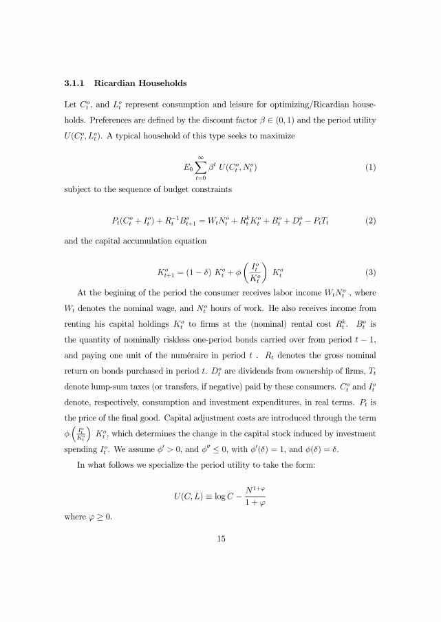
3.1.1 Ricardian Households

Let Cot , and Lot represent consumption and leisure for optimizing/Ricardian house-

holds. Preferences are de…ned by the discount factor (0, 1) and the period utility

U(Cot , Lot ). A typical household of this type seeks to maximize

E0Xt=0

t U(Cot , Not ) (1)

subject to the sequence of budget constraints

Pt(Cot + I

ot ) +R

1t B

ot+1 =WtN

ot +R

ktK

ot +B

ot +D

ot PtTt (2)

and the capital accumulation equation

Kot+1 = (1 ) Ko

t +

µIotKot

¶Kot (3)

At the begining of the period the consumer receives labor income WtNot , where

Wt denotes the nominal wage, and Not hours of work. He also receives income from

renting his capital holdings Kot to …rms at the (nominal) rental cost R

kt . Bot is

the quantity of nominally riskless one-period bonds carried over from period t 1,

and paying one unit of the numéraire in period t . Rt denotes the gross nominal

return on bonds purchased in period t. Dot are dividends from ownership of …rms, Tt

denote lump-sum taxes (or transfers, if negative) paid by these consumers. Cot and Iot

denote, respectively, consumption and investment expenditures, in real terms. Pt is

the price of the …nal good. Capital adjustment costs are introduced through the term³IotKot

´Kot , which determines the change in the capital stock induced by investment

spending Iot . We assume0 > 0, and 00 0, with 0( ) = 1, and ( ) = .

In what follows we specialize the period utility to take the form:

U(C,L) logCN1+

1 +

where 0.

15

References

Aiyagari, R., L.Christiano and M. Eichenbaum (1990): “Output, Employ-

ment and Interest Rate E ects of Government Consumption”, Journal of Mon-

etary Economics, 30, 73-86.

Alesina, A, S. Ardagna, R. Perotti and F. Schiantarelli (2002): “Fiscal

Policy, Profits, and Investment,” American Economic Review, 92 (3), 571-589.

Baxter, M. and R. King (1993): “Fiscal Policy in General Equilibrium”, Amer-

ican Economic Review, 83, 315-334.

Campbell, J. Y. and N. Gregory Mankiw (1989): “Consumption, Income, and

Interest Rates: Reinterpreting the Time Series Evidence,” in O.J. Blanchard

and S. Fischer (eds.), NBERMacroeconomics Annual 1989, 185-216, MIT Press.

Christiano, L. and M. Eichenbaum (1992): “ Current Real Business Cycles

Theories and Aggregate Labor Market Fluctuations”, American Economic Re-

view, 82, 430-450.

Blanchard, O. (2001): Macroeconomics, Prentice Hall.

Blanchard, O. and R. Perotti (2002): “An Empirical Characterization of the

Dynamic E ects of Changes in Government Spending and Taxes on Output,”

Quarterly Journal of Economics,117, 4, 1329-1368.

Bohn, H. (1998): ”The Behavior of Public Debt and Deficits”, The Quarterly

Journal of Economics 113(3), 949-964.

Burnside, C., M. Eichenbaum and J. Fisher (2003): ”Fiscal Shocks and their

Consequences”, NBER WP no 9772.

37

Campbell, J. Y. and N. G. Mankiw (1989): “Consumption, Income, and Inter-

est Rates: Reinterpreting the Time Series Evidence,” in O.J. Blanchard and S.

Fischer (eds.), NBER Macroeconomics Annual 1989, 185-216, MIT Press.

Calvo, G. (1983): “Staggered Prices in a Utility Maximizing Framework”, Journal

of Monetary Economics, 12, 383-398.

Clarida, R., J. Galí and M. Gertler (1999): ” The Science of Monetary

Policy: A New Keynesian Perspective”, Journal of Economic Literature, 37,

1661-1707.

Dotsey, M. (1999): “Structure from Shocks,” Federal Reserve Bank of Richmond,

Working Paper no 99-6.

Dupor, B. (2002): “Interest Rate Policy and Investment with Adjustment Costs,”

mimeo.

Edelberg, W., M. Eichenbaum, and J. Fisher (1999), “Understanding the

E ects of Shocks to Government Purchases,” Review of Economic Dynamics,

2, 166-206.

Fatás, A. and I. Mihov (2001): “The E ects of Fiscal Policy on Consumption

and Employment: Theory and Evidence,” INSEAD, mimeo.

Galí, J., J. D. López-Salido and J. Vallés (2003): “Rule-of- Thumb Con-

sumers and the Design of Interest Rate Rules”, Working Paper 0320, Banco de

España.

Giavazzi, F., and M. Pagano (1990): “Can Severe Fiscal Contractions be Ex-

pansionary? Tales of Two Small European Countries” in O.J. Blanchard and

S. Fischer (eds.), NBER Macroeconomics Annual 1990, MIT Press.

38

Hemming, R., M. Kell and S. Mahfouz (2002): ” The e ectiveness of Fiscal

Policy in Stimulating Economic Activity-A Review of the Literature, IMF WP

no 02/208.

Kim, J. (2000): “Constructing and estimating a realistic optimizing model of mon-

etary policy,” Journal of Monetary Economics, 45, 2, 329-359.

King, R., and M. Watson (1996): “Money, Prices, Interest Rates and the Busi-

ness Cycle” Review of Economics and Statistics, 78, 35-53.

Mankiw, N. G. (2000): “The Savers-Spenders Theory of Fiscal Policy,” American

Economic Review, 90, 2, 120-125.

Mountford, A. and H. Uhlig (2000): “What are the E ects of Fiscal Policy

Shocks?, Discussion Paper 31, Tilburg University, Center for Economic Re-

search.

Perotti, R. (1999): “Fiscal Policy in Good Times and Bad,” Quarterly Journal

of Economics, 114, 4, 1399-1436.

Ramey, V. and M. Shapiro (1998): “Costly Capital Reallocation and the Ef-

fect of Government Spending,” Carnegie-Rochester Conference Series on Public

Policy, 48, 145-194.

Rotemberg, J. and M. Woodford (1992): “Oligopolistic Pricing and the Ef-

fects of Aggregate Demand on Economic Activity”, Journal of Political Econ-

omy, 100, 1153-1297.

Rotemberg, J. and M. Woodford (1997): ”An Optimization Econometric

Framework for the Evaluation of Monetary Policy” in O.J. Blanchard and S.

Fischer (eds.), NBER Macroeconomics Annual 1997, MIT Press.

– (1999):”Interest Rate Rules in an Estimated Sticky Price Model” in J.B. Taylor

(ed.), Monetary Policy Rules, University of Chicago Press and NBER.

39

Taylor, J. B. (1993): “Discretion versus Policy Rules in Practice,” Carnegie

Rochester Conference Series on Public Policy , December 1993, 39, 195-214.

Wolff, E. (1998): ”Recent Trends in the Size Distribution of Household Wealth”,

Journal of Economic Perspectives 12, 131-150.

Woodford, M. (2001): “The Taylor Rule and Optimal Monetary Policy,” Amer-

ican Economic Review Vol. 91, no. 2, 232-237.

Yun, T. (1996): “Nominal Price Rigidity, Money Supply Endogeneity, and Business

Cycles,” Journal of Monetary Economics 37, 345-370.

40

Figure 1. Responses to a Government Spending Shock

Sample Period: 1954:1-1998:4

government spending0 5 10 15 20 25 30 35 40

-0.5

0.0

0.5

1.0

1.5

consumption0 5 10 15 20 25 30 35 40

-0.12

0.00

0.12

0.24

0.36

0.48

hours0 5 10 15 20 25 30 35 40

-0.18

-0.09

0.00

0.09

0.18

0.27

0.36

taxes0 5 10 15 20 25 30 35 40

-0.25

0.00

0.25

0.50

0.75

1.00

1.25

gdp0 5 10 15 20 25 30 35 40

-0.25

0.00

0.25

0.50

investment0 5 10 15 20 25 30 35 40

-1.5

-1.0

-0.5

0.0

0.5

1.0

real wages0 5 10 15 20 25 30 35 40

-0.06

0.00

0.06

0.12

0.18

0.24

defic it0 5 10 15 20 25 30 35 40

-0.6

0.0

0.6

1.2

1.8

41

Figure 2. Determinacy Analysis

Baseline Calibration

indeterminacy

uniqueness

42

Figure 3. Impact Multipliers: Sensitivity to g

Persistence of the Government Spending Shock ( g )

Consumption

Output

Investment

0 0.5 0.9 1

0.0

6.5

43

Figure 4. Impact Multipliers: Sensitivity to g

Alternative Calibrations

Flexible Prices

0 0.5 1-0.5

0

0.5

1No Rule-of-Thumb Consumers

0 0.5 1-0.5

0

0.5

1

Neoclassical

0 0.5 1-0.5

0

0.5

1

Persistence of Government Spending Shock ( g )

Consumption

Output

Investment

Baseline

0 0.5 1-1

0

1

2

3

4

5

44

Figure 5. Impulse Responses to a Government Spending Shock

Neoclassical vs. Baseline Models

government spending

0 4 16 200

0.5

1

output

0 4 16 200

1

2

consumption

0 4 16 20-0.5

0

0.5

1

investment

0 4 16 20-0.1

0

0.1

Horizon

hours

0 4 16 200

1

2

3

Horizon

real wages

0 4 16 20

00.5

11.5

Horizon

taxes

0 5 10 15 200

0.5

1deficit

0 5 10 15 20-0.5

0

0.5

1

o-o-o baseline model -------- neoclassical model

45

Figure 6. Impact Multipliers

Sensitivity to Non-Policy Parameters { , , , }

Sensitivity to

Output

Investment

Consumption

0 0.3 0.5-0.5

0

0.5

1

1.5

2Sensitivity to

0 0.25 0.6 0.75-0.5

0

0.5

1

1.5

2

2.5

Sensitivity to

0.1 1 5 8-0.5

0

0.5

1

1.5

2Sensitivity to

0 0.12 0.3-0.5

0

0.5

1

1.5

2

46

Figure 7. Impact Multipliers

Sensitivity to Policy Parameters { , g, b}

1 1.5 2-2

0

2

4

Investment

ConsumptionOutput

g0 0.2 0.7

-1

0

1

2

b0 0.05 0.2

-1

0

1

2

47