Understanding Neural Network Sample Complexity and ...
89
Understanding Neural Network Sample Complexity and Interpretable Convergence-guaranteed Deep Learning with Polynomial Regression by Matt V. Emschwiller Ing´ enieur diplˆ ome ´ de l’ ´ Ecole polytechnique (B.S. 2017, M.S. 2018) Submitted to the Sloan School of Management in partial fulfillment of the requirements for the degree of MASTER OF SCIENCE IN OPERATIONS RESEARCH at the MASSACHUSETTS INSTITUTE OF TECHNOLOGY May 2020 c 2020 Massachusetts Institute of Technology. All rights reserved. Author ...................................................................................... Sloan School of Management May 1st, 2020 Certified by .................................................................................. Prof. David Gamarnik Nanyang Technological University Professor of Operations Research Thesis Supervisor Accepted by ................................................................................. Prof. Patrick Jaillet Dugald C. Jackson Professor, Department of Electrical Engineering and Computer Science Co-Director, Operations Research Center 1
Transcript of Understanding Neural Network Sample Complexity and ...

Understanding Neural Network Sample Complexity and Interpretable Convergence-guaranteed Deep Learning with
Polynomial Regression
by
Matt V. Emschwiller
Ingenieur diplome de l’Ecole polytechnique (B.S. 2017, M.S. 2018)
Submitted to the Sloan School of Managementin partial fulfillment of the requirements for the degree of
MASTER OF SCIENCE IN OPERATIONS RESEARCH
at the
MASSACHUSETTS INSTITUTE OF TECHNOLOGY
May 2020
c© 2020 Massachusetts Institute of Technology. All rights reserved.
Author . . . . . . . . . . . . . . . . . . . . . . . . . . . . . . . . . . . . . . . . . . . . . . . . . . . . . . . . . . . . . . . . . . . . . . . . . . . . . . . . . . . . . .Sloan School of Management
May 1st, 2020
Certified by . . . . . . . . . . . . . . . . . . . . . . . . . . . . . . . . . . . . . . . . . . . . . . . . . . . . . . . . . . . . . . . . . . . . . . . . . . . . . . . . . .Prof. David Gamarnik
Nanyang Technological University Professor of Operations ResearchThesis Supervisor
Accepted by . . . . . . . . . . . . . . . . . . . . . . . . . . . . . . . . . . . . . . . . . . . . . . . . . . . . . . . . . . . . . . . . . . . . . . . . . . . . . . . . .Prof. Patrick Jaillet
Dugald C. Jackson Professor, Department of Electrical Engineering and Computer ScienceCo-Director, Operations Research Center
1

2

Understanding Neural Network Sample Complexity andInterpretable Convergence-guaranteed Deep Learning with
Polynomial Regression
by
Matt V. Emschwiller
Submitted to the Sloan School of Managementon May 1st, 2020 in partial fulfillment of the
requirements for the degree ofMaster of Science in Operations Research
Abstract
We first study the sample complexity of one-layer neural networks, namely the number of ex-amples that are needed in the training set for such models to be able to learn meaningfulinformation out-of-sample. We empirically derive quantitative relationships between the sam-ple complexity and the parameters of the network, such as its input dimension and its width.Then, we introduce polynomial regression as a proxy for neural networks through a polynomialapproximation of their activation function. This method operates in the lifted space of tensorproducts of input variables, and is trained by simply optimizing a standard least squares ob-jective in this space. We study the scalability of polynomial regression, and are able to designa bagging-type algorithm to successfully train it. The method achieves competitive accuracyon simple image datasets while being more simple. We also demonstrate that it is more robustand more interpretable that existing approaches. It also offers more convergence guaranteesduring training. Finally, we empirically show that the widely-used Stochastic Gradient Descentalgorithm makes the weights of the trained neural networks converge to the optimal polynomialregression weights.
Thesis Supervisor: Prof. David GamarnikNanyang Technological University Professor of Operations Research
3

4

Contents
1 Introduction 9
1.1 Background . . . . . . . . . . . . . . . . . . . . . . . . . . . . . . . . . . . . . . . 9
1.1.1 Deep learning . . . . . . . . . . . . . . . . . . . . . . . . . . . . . . . . . . 9
1.1.2 Expressiveness power of neural networks . . . . . . . . . . . . . . . . . . . 11
1.1.3 Algorithmic considerations . . . . . . . . . . . . . . . . . . . . . . . . . . 13
1.1.4 Gradient-based methods on the population loss function . . . . . . . . . . 14
1.1.5 Gradient-based methods on the empirical loss function . . . . . . . . . . . 15
1.1.6 Energy landscape of neural networks . . . . . . . . . . . . . . . . . . . . . 17
1.1.7 Neural networks robustness to noise . . . . . . . . . . . . . . . . . . . . . 23
1.1.8 Polynomial regression . . . . . . . . . . . . . . . . . . . . . . . . . . . . . 24
1.2 Organization of the report . . . . . . . . . . . . . . . . . . . . . . . . . . . . . . . 25
2 Sample complexity of neural networks 27
2.1 General setup . . . . . . . . . . . . . . . . . . . . . . . . . . . . . . . . . . . . . . 27
2.2 Experiments . . . . . . . . . . . . . . . . . . . . . . . . . . . . . . . . . . . . . . . 28
2.3 Methods . . . . . . . . . . . . . . . . . . . . . . . . . . . . . . . . . . . . . . . . . 30
2.4 Results . . . . . . . . . . . . . . . . . . . . . . . . . . . . . . . . . . . . . . . . . . 31
2.4.1 Algorithmic setup . . . . . . . . . . . . . . . . . . . . . . . . . . . . . . . 31
2.4.2 Recovery precision . . . . . . . . . . . . . . . . . . . . . . . . . . . . . . . 32
2.4.3 Sample complexity . . . . . . . . . . . . . . . . . . . . . . . . . . . . . . . 35
3 Polynomial regression 43
3.1 General setup . . . . . . . . . . . . . . . . . . . . . . . . . . . . . . . . . . . . . . 43
3.2 Testing on synthetic data . . . . . . . . . . . . . . . . . . . . . . . . . . . . . . . 45
3.2.1 Construction of the synthetic dataset . . . . . . . . . . . . . . . . . . . . . 45
3.2.2 Impact of d and m . . . . . . . . . . . . . . . . . . . . . . . . . . . . . . . 46
5

CONTENTS
3.2.3 Sample complexity . . . . . . . . . . . . . . . . . . . . . . . . . . . . . . . 47
3.2.4 Approximating activation functions . . . . . . . . . . . . . . . . . . . . . . 48
3.3 Testing on real data – setup and benchmarks . . . . . . . . . . . . . . . . . . . . 49
3.3.1 Setup . . . . . . . . . . . . . . . . . . . . . . . . . . . . . . . . . . . . . . 49
3.3.2 State-of-the-art models . . . . . . . . . . . . . . . . . . . . . . . . . . . . 49
3.3.3 A deep learning inspired approach . . . . . . . . . . . . . . . . . . . . . . 50
3.3.4 A dimensionality reduction approach . . . . . . . . . . . . . . . . . . . . . 52
3.4 Fitting polynomial regression . . . . . . . . . . . . . . . . . . . . . . . . . . . . . 57
3.4.1 Challenges and scalability of the method . . . . . . . . . . . . . . . . . . . 57
3.4.2 Setup . . . . . . . . . . . . . . . . . . . . . . . . . . . . . . . . . . . . . . 58
3.4.3 Introduction of batched linear regression as a scalable fitting method . . . 59
3.4.4 Comparison to benchmarks . . . . . . . . . . . . . . . . . . . . . . . . . . 62
3.4.5 Comparison to exact methods when tractable . . . . . . . . . . . . . . . . 63
3.5 Understanding gradient descent behavior . . . . . . . . . . . . . . . . . . . . . . . 65
3.6 Advantages . . . . . . . . . . . . . . . . . . . . . . . . . . . . . . . . . . . . . . . 72
3.6.1 Interpretability . . . . . . . . . . . . . . . . . . . . . . . . . . . . . . . . . 72
3.6.2 Robustness to noise . . . . . . . . . . . . . . . . . . . . . . . . . . . . . . 76
4 Conclusion 81
6

List of Figures
1.1 Standard activation functions. . . . . . . . . . . . . . . . . . . . . . . . . . . . . . 9
1.2 Prediction landscape vs. first two input coordinates for a random one-layer neural
network. . . . . . . . . . . . . . . . . . . . . . . . . . . . . . . . . . . . . . . . . . 19
1.3 Empirical loss landscape vs. first two weights for a random one-layer neural
network. . . . . . . . . . . . . . . . . . . . . . . . . . . . . . . . . . . . . . . . . . 20
2.1 One-layer neural network architecture (from [ZYWG18a]). . . . . . . . . . . . . . 27
2.2 Recovery R2 vs. input dimension, against network parameters. . . . . . . . . . . 33
2.3 Recovery R2 vs. hidden dimension, against network parameters. . . . . . . . . . 34
2.4 Recovery R2 vs. sample size, against network parameters. . . . . . . . . . . . . . 35
2.5 Sample complexity vs. input dimension and best linear fits, without dichotomy. . 35
2.6 Sample complexity vs. hidden dimension and best linear fits, without dichotomy. 36
2.7 Recovery probability vs. sample size, against network parameters. . . . . . . . . 37
2.8 Sample complexity trials vs. hidden dimension, with dichotomy. . . . . . . . . . . 39
2.9 Sample complexity trials vs. hidden dimension, best logarithmic linear fit, with
dichotomy. . . . . . . . . . . . . . . . . . . . . . . . . . . . . . . . . . . . . . . . . 40
2.10 Sample complexity vs. input dimension, trials and best linear fit, with dichotomy. 41
3.1 Performance of polynomial regression for synthetic datasets vs. network param-
eters. . . . . . . . . . . . . . . . . . . . . . . . . . . . . . . . . . . . . . . . . . . . 47
3.2 Generalization gap vs. ratio of dataset size to number of polynomial regression
features. . . . . . . . . . . . . . . . . . . . . . . . . . . . . . . . . . . . . . . . . . 47
3.3 Example images from datasets used. . . . . . . . . . . . . . . . . . . . . . . . . . 49
3.4 LeNet5 architecture. . . . . . . . . . . . . . . . . . . . . . . . . . . . . . . . . . . 51
3.5 Out-of-sample accuracy of the CNN model during the training process, zoomed. . 52
7

LIST OF FIGURES
3.6 In-sample and out-of-sample accuracy of the polynomial regression model vs.
number of principal components. . . . . . . . . . . . . . . . . . . . . . . . . . . . 53
3.7 Most important PCA components. . . . . . . . . . . . . . . . . . . . . . . . . . . 54
3.8 Original image and DCT encoding. . . . . . . . . . . . . . . . . . . . . . . . . . . 55
3.9 Thresholded DCT encoding and decoded image. . . . . . . . . . . . . . . . . . . 55
3.10 Probability that each pixel appears in the DCT-encoded and thresholded version
of an image, across the dataset. . . . . . . . . . . . . . . . . . . . . . . . . . . . . 57
3.11 Out-of-sample accuracy of individual and cumulative batched linear regression
models. . . . . . . . . . . . . . . . . . . . . . . . . . . . . . . . . . . . . . . . . . 61
3.12 In-sample and out-of-sample accuracy of the cumulative batched linear regression
model. . . . . . . . . . . . . . . . . . . . . . . . . . . . . . . . . . . . . . . . . . . 61
3.13 Polynomial approximation of ReLU activation. . . . . . . . . . . . . . . . . . . . 67
3.14 In-sample and out-of-sample comparison of student network and polynomial re-
gression output. . . . . . . . . . . . . . . . . . . . . . . . . . . . . . . . . . . . . . 68
3.15 Neural network “equivalent” tensor weights vs. polynomial regression weights
with ReLU L2 polynomial approximation. . . . . . . . . . . . . . . . . . . . . . . 69
3.16 Neural network “equivalent” tensor weights vs. polynomial regression weights
with ReLU L∞ polynomial approximation. . . . . . . . . . . . . . . . . . . . . . 69
3.17 Polynomial approximation of ReLU activation (priors and posterior). . . . . . . . 71
3.18 Neural network “equivalent” tensor weights vs. polynomial regression weights
with ReLU posterior polynomial approximation. . . . . . . . . . . . . . . . . . . 71
3.19 Interpretation of degree 1 coefficients for polynomial regression. . . . . . . . . . . 73
3.20 Interpretation of degree 2 coefficients for polynomial regression. . . . . . . . . . . 75
3.21 Images after applying the global noise modification, for σ = 0.3. . . . . . . . . . . 76
3.22 Images after applying the local noise modification, for A = 100. . . . . . . . . . . 77
3.23 Accuracy and relative accuracy drop vs. noise standard deviation σ in the global
noise setting. . . . . . . . . . . . . . . . . . . . . . . . . . . . . . . . . . . . . . . 78
3.24 Accuracy and relative accuracy drop vs. patch area A in the local noise setting. . 79
8

Chapter 1
Introduction
1.1 Background
1.1.1 Deep learning
For the past years, deep neural networks have shown state-of-the-art performance in tasks such
as image recognition ([KSH12]), speech classification ([HDY+12, MHN13, ZRM+13]), machine
translation ([BCB15]), and even complex games like Go ([SHM+16]). ReLU neural networks
([GBB11]), where the activation of each neuron is defined as σ(x) = maxx, 0, have appeared
to be favored by most of the literature.
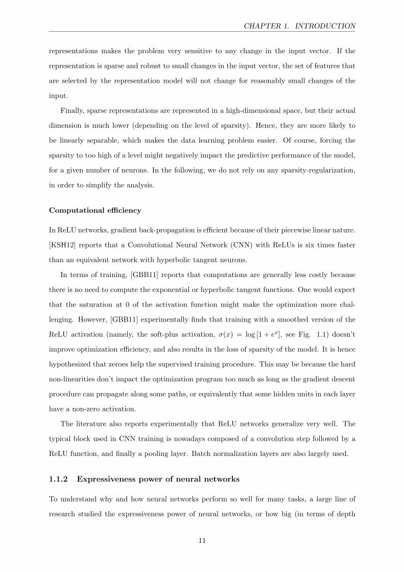
Figure 1.1: Standard activation functions.
These networks possess several attractive computational properties which are worth men-
tioning and analyzing, and which justify the choice of the representation studied here.
9

CHAPTER 1. INTRODUCTION
Vanishing gradient
Compared to networks that use sigmoid activation, ReLU neural networks are less affected
([GBB11]) by the vanishing gradient problem ([BSF94, Hoc98]). This phenomenon appears
when using an activation function such as the sigmoid function (σ(x) = 11+e−x ) or the hyperbolic
tangent (σ(x) = tanh(x)). These two functions have a gradient that shrinks towards 0 at both
x→ +∞ and x→ −∞. The gradient value vanishing causes the training process to effectively
come to a stop (the updates of the weights of the network become infinitesimal) after a certain
number of epochs. In ReLU networks, the gradient of the activation function is piecewise
constant, and doesn’t vanish at x → +∞. Moreover, as shown in [HN10], ReLU networks can
be seen as a representation of an exponential number of linear models that share parameters.
The only non-linearity comes from which paths are active from the first layer of the network
to the last one (a path of neurons is defined as “active” if all neurons along this path have a
non-zero ReLU activation). Once we know which paths are active, it is possible to reformulate
the function computed by the network as mentioned. Because of this linearity, gradients flow
well on the neurons paths that are active, which facilitates mathematical investigation.
Sparsity
ReLU neurons also encourage sparsity in the hidden layers ([GBB11]), which make the effective
number of parameters of the network go down, and pushes the network towards the path of
interpretability. With random initialization of the network weights, the proportion of hidden
units with zero activation will converge towards 50% as the network width increases, and this
percentage can be even further increased with a sparsity-inducing regularization. For example,
the Lasso regularization ([Tib96]) is one such sparsity-inducing regularization, since it adds
a term λ ‖W‖1 in the optimization program. Sparsity has more generally become a major
subject of interest for computational cognitive sciences and machine learning, as well as for
signal processing and statistics (see [CT05] for example).
Sparsity in neural networks can also allow the networks to control their effective dimension-
ality, by increasing or decreasing the number of active hidden units. Different inputs might
contain different levels of information and would thus need different treatment in terms of the
size of the architecture that tries to analyze it. According to [Ben09], an objective of machine
learning is to separate the factors explaining the variations in the data (similar to what a Prin-
cipal Component Analysis analysis would do, but in a more complex approach). Having dense
10
CHAPTER 1. INTRODUCTION
representations makes the problem very sensitive to any change in the input vector. If the
representation is sparse and robust to small changes in the input vector, the set of features that
are selected by the representation model will not change for reasonably small changes of the
input.
Finally, sparse representations are represented in a high-dimensional space, but their actual
dimension is much lower (depending on the level of sparsity). Hence, they are more likely to
be linearly separable, which makes the data learning problem easier. Of course, forcing the
sparsity to too high of a level might negatively impact the predictive performance of the model,
for a given number of neurons. In the following, we do not rely on any sparsity-regularization,
in order to simplify the analysis.
Computational efficiency
In ReLU networks, gradient back-propagation is efficient because of their piecewise linear nature.
[KSH12] reports that a Convolutional Neural Network (CNN) with ReLUs is six times faster
than an equivalent network with hyperbolic tangent neurons.
In terms of training, [GBB11] reports that computations are generally less costly because
there is no need to compute the exponential or hyperbolic tangent functions. One would expect
that the saturation at 0 of the activation function might make the optimization more chal-
lenging. However, [GBB11] experimentally finds that training with a smoothed version of the
ReLU activation (namely, the soft-plus activation, σ(x) = log [1 + ex], see Fig. 1.1) doesn’t
improve optimization efficiency, and also results in the loss of sparsity of the model. It is hence
hypothesized that zeroes help the supervised training procedure. This may be because the hard
non-linearities don’t impact the optimization program too much as long as the gradient descent
procedure can propagate along some paths, or equivalently that some hidden units in each layer
have a non-zero activation.
The literature also reports experimentally that ReLU networks generalize very well. The
typical block used in CNN training is nowadays composed of a convolution step followed by a
ReLU function, and finally a pooling layer. Batch normalization layers are also largely used.
1.1.2 Expressiveness power of neural networks
To understand why and how neural networks perform so well for many tasks, a large line of
research studied the expressiveness power of neural networks, or how big (in terms of depth
11

CHAPTER 1. INTRODUCTION
and width) a network needs to be in order to succeed in some task, as well as if it can achieve
a given task or not. This directly relates to universal approximation theory, which studies how
some classes of functions can be approximated by other classes of functions (or more simply
put, which classes of functions are dense in some sets). From a machine learning perspective,
universal approximation theory is only the first step: efficiency, or the size of the neural network
required to achieve the approximation, is also crucial. Let us first focus on the former.
It is well-known ([Cyb89]) that classes of functions similar to the one we consider in this
paper are rich enough to approximate “reasonable” functions arbitrarily well. Those classes of
function are what we call “one-layer” neural networks, namely neural networks with depth 1
(one hidden layer between the input and the output) and varying width.
Definition 1.1.1. A function σ : R 7→ R is said to be sigmoidal if σ(x) −−−−→x→−∞
0 and
σ(x) −−−−→x→+∞
1.
If σ is also continuous, and f is L2 with respect to the distribution of the inputs X (meaning
E[f(X)2
]< ∞), then the following holds [Cyb89] (the original version actually states the
following for functions f defined on compact sets, not R, and without the L2 assumption on
f(X)):
∀ε > 0 ∃m ∈ N s.t. infW
E
[∣∣∣∣∣f(X)− 1
m
m∑i=1
σ((W>X)i)
∣∣∣∣∣]≤ ε. (1.1)
This means that one hidden layer neural networks can approximate arbitrarily well any smooth
function, as long as the width is large enough. A key observation is that this theorem doesn’t
state how large m can become as ε decreases. In practice, it is often observed that m seems to get
too large to be computationally efficient, and that is why, in practice, people increase the depth
of the network instead of keeping only one hidden layer. However, theoretically, nothing says
at this point that one-layer neural networks with sigmoid and continuous activation functions
are too limited to approximate any reasonably shaped function well.
[Hor91] improved the result obtained in [Cyb89], proving that, as long as the activation func-
tion is bounded and non-constant, then any one-layer neural network with width large enough
can approximate arbitrarily well any function f such that E [f(X)p] < ∞ with respect to the
Lp norm. If the activation function is also continuous, then the network can approximate any
continuous function on compact subsets. Finally, if the activation function is unbounded and
non-constant, a similar density result on Lp functions is established. By removing the assump-
tions that the activation function had to be integrable, sigmoidal or monotone for example,
12

CHAPTER 1. INTRODUCTION
[Hor91] results facilitate the consideration of ReLU activations, which we do in most parts of
this report.
When it comes to the width required to achieve such approximation, [CSS16] proves that all
functions (up to a negligible set of them) that can be approximated by a deep (with more than
one layer) neural network of polynomial size require an exponential size in order to be approx-
imated by a one-layer neural network. This result obviously doesn’t contradict the universal
approximation result for one-layer neural networks, but shows that these simplistic networks
might not be best-fitted to approximate all functions efficiently. [Tel16] proves a similar result,
by showing that there exists neural networks of polynomial depth O(k3) and of width O(1) that
can’t be approximated by any network of linear depth O(k), unless their width grows expo-
nentially with k. This result is valid for a class of activation functions called “semi-algebraic
gates,” which includes ReLU activations and max-pooling activations (for CNNs).
To further study the impact of depth, [AGMR16, PLR+16, RPK+16] showed how the com-
plexity of the function computed by a deep neural network grows exponentially with the depth
of such a network. In particular, this provides a hint that sample complexity (the number of
training examples required to approximate the true function) should also grow very fast with
depth. We will however focus on one-layer neural networks, and avoid this exponential grow
(with depth) of the complexity of the class of networks considered.
[LPW+17] studied universal approximation results for width-bounded ReLU networks. They
show that these networks are also universal approximators (for a varying depth) as long as the
width of the networks is at least d+ 4 (with d the network’s input dimension). Also, it appears
that not all functions can be approximated by the same class of network with width equal to d.
A symmetric result (to the ones in [CSS16, Tel16]) shows that there exists classes of wide and
shallow networks that can’t be approximated by deep and narrow networks, as long as the depth
is no more than a polynomial bound. Experimentally, [LPW+17] finds that these networks can
however be approximated if depth is allowed to grow higher than this polynomial bound.
1.1.3 Algorithmic considerations
Studying the expressive power of neural networks is not enough to explain the empirical success
of deep learning. In fact, even if universal approximation theorems are available, one still
has to find, in practice, the actual network that is close to the observed data, which is an
algorithmic challenge. Although neural networks are successfully trained using simple gradient-
13

CHAPTER 1. INTRODUCTION
based methods (such as gradient descent or stochastic gradient descent), from a theoretical
perspective it is known that, in general, learning neural networks is hard in the worst-case.
[Sha16] establishes that even if the target function is “nice” (shallow ReLU networks for
example), there exist adversarially difficult input distributions to learn. There also exists “nice”
target function classes (of the form ψ(〈w, x〉) for example) that are difficult to learn even if the
input distribution is well-behaved. [SSSS17a] exhibits some of these target function classes for
which gradient-based methods fail, while [SSSS17b] argues that weight sharing is crucial for
successful optimization, presenting an interesting case for CNNs.
[ZLWJ17] studies the learnability of L1 bounded (where the weights for each layer have a
bounded L1 norm) neural networks, and shows that learning these network is polynomial in n
(the number of training examples) and d (the input dimension) but exponential in the error that
we want to achieve. This exponential dependence is shown to be avoidable in very simplistic
cases, for example when data-points are linearly separable.
Even for one-layer neural networks as considered here, it is argued in [AHW96] that the
number of local minima on the empirical loss function can grow exponentially with the dimen-
sion. However, this result doesn’t rule out the possibility that those local minima might achieve
a value very close to the one of the global minima.
Finally, NP-completeness of neural network training is shown to hold for 2− and 3−node
neural networks with a thresholding activation function (f(x) = 2 · 1〈w,x〉>0 − 1). The result
also holds for k hidden nodes, as long as k is bounded by some polynomial of the size of the
dataset, and the output is the product of the activations at every node.
Despite facing those theoretical difficulties, a large number of studies such as [SA14, KKSK11,
GKKT16, AGMR16, ZLWJ15, KS09, JSA15] have been trying to develop new algorithms able
to learn neural network with provable guarantees. However, none of these algorithms is similar
to a gradient-based method, the most widely used type of optimization in machine learning at
this point in time. Hence these papers don’t explain the apparent efficiency of gradient-based
methods to train neural networks.
1.1.4 Gradient-based methods on the population loss function
Even if the above-mentioned complexity results each have some specific assumptions that might
not apply to the case considered here, they hint at the fact that algorithmic questions are
interesting to consider. In fact, learning neural networks is proven to be hard theoretically, but
14
CHAPTER 1. INTRODUCTION
is successful in most cases in practice. Since the algorithms used in the real-world are gradient-
based, we choose to experimentally study the behavior of this type of algorithm, and how it
turns out to be successful at efficiently achieving a supposedly almost unachievable task. There
has been a lot of recent work on recovery guarantees with gradient-based methods, whether
based on the population or the empirical loss function.
Some progress has been achieved on these guarantees based on population loss function
(the expected risk, not the empirical risk). Among this work, many studies have focused on
CNNs, and how to learn convolutional filters. [DLT17a] showed that, for one-layer CNNs with
ReLU activation, when the labels in the dataset come from a teacher network of the same
type of architecture, the learner network can recover the wrong network (there exist spurious
local minima in the population loss function). However, it is argued that properly randomly
initialized gradient descent procedures still seem to recover the teacher network from which the
dataset was generated, and by restarting the procedure many times, the recovery probability
can be boosted to 1. This setup of recovering a teacher network is very similar to the one we
use in this report, albeit with some differences. [BG17] is very similar and reports a polynomial
rate of convergence for gradient descent procedures when the input distribution is Gaussian.
[DLT17b] reports the same kind of results, with fewer assumptions (in particular, the Gaussian
form of the input distribution is not needed) on the convergence of the Stochastic Gradient
Descent (SGD) procedure. Finally, [LY17] reports SGD convergence for one-layer ReLU neural
networks with identity mapping (adding the input X to the pre-activation output of the hidden
layer W>X) and for Gaussian input distributions.
1.1.5 Gradient-based methods on the empirical loss function
When using deep learning in practice, neural network training is largely based on the empirical
loss function, because there is obviously no access to the population one. Of course, as the
sample size grows, the former converges to the latter. Recent studies have been looking at
gradient-based methods to train neural networks, which employ empirical loss minimization.
While some of them apply to the case considered here, some of them don’t directly apply.
[ZSJ+17] provides conditions on the activation function (which are verified by the ReLU func-
tion) that lead to local strong convexity of the loss objective in the neighborhood of the true
parameters. For activation functions that are smooth (which is not the case for the ReLU func-
tion), a local linear convergence rate is proven, and the sample complexity and computational
15

CHAPTER 1. INTRODUCTION
complexity are shown to be linear in the input dimension d and logarithmic in the recovery
precision. Similarly, [FCL18] establishes that, if inputs are Gaussian, the empirical loss func-
tion is strongly convex and uniformly smooth in a local neighborhood of the true parameters.
Using the tensor method, gradient descent is initialized in this neighborhood and the conver-
gence rates are again shown to be linear. However, this analysis is only derived for the sigmoid
activation function, and does not apply to the ReLU activation function. [SJL17] studies a
similar problem in the over-parametrized regime (fewer observations than parameters), and de-
rives some interesting properties of the optimization landscape but with restrictive assumption
on the activation function (sometimes quadratic, sometimes differentiable). Within this set
of assumptions, a similar linear local convergence rate is established when gradient descent is
properly initialized.
Another set of studies looked at the case of deep linear networks, in which there is no
activation function. The formula defining the output of the network is then:
F (X) = Wk...W1X (1.2)
Fundamentally, minimizing a loss with this type of network is the same as doing a linear
regression to find the weight parameter W = Wk...W1. However, using gradient descent to
minimize the error is not equivalent to linear regression, since the training is done on all the
weights separately, whereas linear regression optimizes W directly. Understanding this case
might be helpful to understand the general case of activation functions other than identity.
[Sha18] claims that, for these networks, randomly initialized gradient descent procedures will
display a number of iterations growing exponentially with the depth of the network. Similarly,
[ACGH18] extends results found in [BHL18] and proves linear convergence rates of gradient-
descent procedures, but with some constraints on both the network (whose width has to be
larger than its input dimension) and the initialization procedure.
Some other studies actually apply to the ReLU activation function, which is more interesting
for the case studied here, and more widely used in practice. [Sol17] extends [SJL17] by studying
the same problem for the ReLU activation function in the over-parametrized case, and when the
weight vector is constrained to be in some closed set (which is supposed to be known using side
“oracle” information on the weights). The rates in terms of sample or computational complexity
are the same as in [ZSJ+17]. However, their gradient descent approach has a projection step on
16

CHAPTER 1. INTRODUCTION
this closed set, which depends on the true parameters, and is hence not doable in practice. That
makes the algorithm less useful in practice. [DZPS18] uses a less restrictive framework to analyze
convergence of gradient descent for ReLU networks. According to their study, no criterion on
gradient descent initialization is required (it is randomly done), and even the dataset doesn’t
need to come from a teacher network. The gradient descent procedure would converge, for any
dataset (xi, yi)i=1...n, even a dataset not generated from a network of a similar architecture,
which is surprising. One requirement, however, is that the network must be quite large, of
order Ω(
n6
λ40δ3
)where n is the size of the dataset, λ0 the minimum eigenvalue of the stationary
limit of the matrix H(t) that determines the SGD optimization step at time t – i.e. dy(t)dt =
H(t)(y(t)− y(t)), where y is the target, and y the prediction – and δ the recovery error. Based
on what is observed in practice, this result is not satisfactory because one can actually recover
a teacher network with a learner network of width much smaller than the bound derived here,
which means that the bound is very loose and thus not very useful. Finally, [ZYWG18b] extends
[FCL18] in the case of the ReLU activation function. A locally linear convergence rate is derived
when the initial position of the gradient descent procedure is close enough to the true parameter.
This initialization is done using, again, the tensor method, and the sample complexity is proven
to be of order d up to logarithmic factors, but of enormous order in terms of width (to the
ninth power), which is again not satisfactory empirically speaking. Most of these studies also
completely lack empirical verification of their theoretical study, or display empirical results that
are not very significant (not enough sampling, not enough experiments, etc.). To the best of our
knowledge, there haven’t been any extensive empirical studies on how easily gradient descent
recovers the true parameters of a teacher network, depending on the dimension and the width
of the networks. This is what we will focus on in the first part of the report.
1.1.6 Energy landscape of neural networks
Quite recently, nice results have been obtained on first-order optimization problems for solving
non-convex optimization programs efficiently. [JGN+17] introduces a modified form of gradient-
descent that can escape saddle-points at a minimal cost. At each step of the gradient-descent
procedure, noise (with a fine-tuned scale) is added to the current point, in order to move
away from it and hopefully escape the blocking situation in which the algorithm ended up.
Similarly, [GHJY15] analyzed the convergence of SGD on non-convex objective functions with
an exponential number of local minima and saddle points. Convergence (to a local minima
17

CHAPTER 1. INTRODUCTION
whose value is very close to the global minima) is shown to happen in a polynomial number of
iterations.
Following these results, a large portion of the research field started trying to understand
deep or shallow networks by giving characterizations of their energy landscapes, or equivalently
properties of the minima that are present in the loss functions at stake here. One of the earliest
work on the topic was done in [CHM+15] in 2015. The connection between the loss functions
seen in the training of deep fully-connected neural networks and the Hamiltonian of the spherical
spin-glass model were made clearer, however only under some extremely strong assumptions.
The first reformulation of the network, initially written as
f(X) = σ(W>Kσ(W>K−1...σ(W>1 X)))...), (1.3)
where σ is the activation function, was re-organized as a polynomial function of the weights of
the network, with an number of monomials equal to the number of paths from the input layer
to the output layer, and degree equal to the depth K:
f(X) =d∑i=1
γ∑j=1
Xi,jAi,j
K∏k=1
w(k)i,j , (1.4)
where d is the size of the input layer, γ the number of paths from one unit of the input layer
to the output layer, X a matrix of copies of the input vector, w(k) the weights in the kth
layer, and finally A a binary variable to index if a path (i, j) is active or not (i.e. if all of
the ReLU activations along the path are non-zero). Under strong assumptions such as the
independence between X and A, the authors were able to re-formulate this function as a spin-
glass Hamiltonian.
The key idea is that, once reformulated as a spin-glass model, previous studies like the ones
in [ABAC10, ABA13] that already analyzed the Hamiltonian of such systems can be used to
derive the properties of the landscape of the loss function. Based on the empirical observations
formulated by researchers in the late 1980s and early 1990s, according to which convergence
of small networks was very unstable, contrary to multi-layer networks whose convergence was
more stable (it still found local minima, but much closer to the global minima than for small
networks), a suggestion was made that, for multi-layer neural networks, local minima were
numerous and easy to find but also almost equivalent in performance on the test set to any
global optimum. Using past spin-glass studies, the authors were able to prove many interesting
18

CHAPTER 1. INTRODUCTION
facts:
• the energy landscape of large networks have many local minima that are roughly equivalent
to any global minima (have a similar loss).
• these local minima are likely to be heavily degenerate, with many eigenvalues of the
Hessian being close to 0.
• the probability of finding a local minimum with high test error increases as the network
becomes smaller.
Despite having very interesting conclusions, this study is challenging to use in practice be-
cause of its reliance on assumptions that are too strong and unrealistic, a limitation that was
acknowledged in the paper.
A few quick numerical experiments are enough to understand how difficult the task of
analyzing the energy landscape of neural networks is, even for one-layer networks. We looked
at the loss functions as well as the output of the network, as a function of the first two weights
in the hidden layer of a randomly selected neural network. We also looked at their dependency
on the first two coordinates of the input vector. We can either make all the weights vary at
the same time by sampling them for each step, or fix all weights except the first two, and make
those two vary randomly.
(a) first two input coordinates varying (b) all input coordinates varying
Figure 1.2: Prediction landscape vs. first two input coordinates for a random one-layer neural network.
The results are as expected. The output of the network is shown in Fig. 1.2, in which
we see that the network is indeed a convex function as a function of the first two coordinates
of the input, with the other ones fixed. However, as soon as other coordinates start varying
19

CHAPTER 1. INTRODUCTION
(a) first two weights varying (b) all weights varying
Figure 1.3: Empirical loss landscape vs. first two weights for a random one-layer neural network.
too, the correlation structure of the network (implied by the connection of the different input
coordinates with each other when aggregating the hidden-layer intermediary results to form
the final prediction) starts to kick-in and makes the function computed by the network highly
non-convex and non-concave. The same story goes for the loss (here, we used the quadratic
loss), as shown in Fig. 1.3. When restricting the loss as a function of the first two weights in
the hidden layer, it indeed becomes convex. That would make a case for training the network
only on two weights at a time. However, once more weights are added in the process, the
correlation between hidden units starts having an effect, and the loss becomes non-smooth. A
very simple idea would be to train the network two weights at a time in order to make sure
that each optimization process was convex. However, the end of this process would certainly
not yield the desired global optimum of the loss function, because this training process would
ignore the correlation structure that the networks imposes between the weights (the class of
networks trained this way would be clearly less expressive than the class of networks trained on
all weights simultaneously).
In [SS16], the quality of the optimization starting point is studied. Under certain conditions,
the training process benefits from a more favorable environment. These conditions include the
existence of a monotonically decreasing path from the starting point to a global minimum,
or having a high chance of initializing the process in an energy basin with a small minimum.
Such properties are shown to be more likely in over-specified networks (in terms of number of
parameters). However, these assumptions are extremely difficult to verify in practice, and hence
experimenting with these properties to gain insight is quite challenging.
[MMN18] takes an interesting approach to study the landscape of two-layer neural networks,
20
CHAPTER 1. INTRODUCTION
by focusing on the statistical physics aspect of the dynamics of the weights in the network during
training, when the number of units in the hidden-layer, denoted m, goes to infinity (“large-
width” networks). In this regime, called the mean-field regime, it is traditionally assumed that
we can replace the parameters of the network by a density ρ. It is also assumed that any averages
over the weights of the network can be replaced by the corresponding expectation under the
density ρ. This regime allows one to transform the function computed by the network, which
is re-written:
f(x; ρ) =
∫σ∗(x; θ)ρ(dθ), (1.5)
where σ∗(x; θ) = σ(〈w, x〉 + b), with θ = (w, b). The authors focus on understanding the
convergence problem, or how the weights of the network move during training, as well as the
time (in terms of steps) it takes for the optimization algorithm (in this case, SGD) to converge.
Defining the objective function as the mean-squared loss, the loss function L can be re-written
in an infinite dimensional space, as a function of the density of the parameters, when the width
of the network goes to infinity:
L(ρ) = Cste +
∫V (θ)ρ(dθ) +
∫U(θ, θ′)ρ(dθ)ρ(dθ′), (1.6)
for some functions V and U . It is shown that instead of minimizing the risk with respect
to the parameters (θ1, ..., θm), it can be minimized in the space of distributions. Then, to
recover optimal parameters for the two-layer neural network, drawing independent values from
the optimal distribution ρ∗ (minimizing L) would be enough. The crucial aspect is that, since
U(·, ·) is positive semi-definite, it is easily obtained that L becomes convex in this mean-field
limit, which is key to understanding the energy landscape of the network.
In terms of convergence, it is shown that the distribution of the weights converges, when
the width of network grows, to a stationary distribution that is defined by some well-studied
PDE. This distribution is shown to verify an approximate regularization relationship with time,
where the regularization term is the L2-Wasserstein metric.
[MMN18] also shows that, roughly speaking, the energy landscape doesn’t change as the
width of the network grows, as long as the input dimension d stays small compared to it. Hence
if the above-mentioned PDE converges close to an optimum in time t, then this time might
depend on d, but not on m, which doesn’t appear in the PDE. Hence the out-of-sample loss
would be independent of m using a number of samples not growing as fast as m, although one
21

CHAPTER 1. INTRODUCTION
would usually assume that a bigger number of training examples would be required for bigger
networks. This is one of the effects we will study in this report. As [SS18] states, the neural
network converges, when m→∞, in probability, to a deterministic model, despite the fact that
it had been randomly initialized and trained on random sequence of data via SGD.
Other recent studies have focused on studying the behavior of simpler neural networks, for
which the activation of each neuron is simply the identity. Those networks are called “linear
neural networks.” Fundamentally, they target the same thing as a linear regression, but SGD
is used to train them. In a theoretical work, [Kaw16] proved that, for such deep linear neural
networks, and for any depth or width, the squared loss function is indeed, as expected, non-
convex and non-concave, but that every local minimum is also a global minimum. The only
problematic points are saddle points, and they exist only for networks with depth larger than 3.
[HM16] chose to take a more optimization-based point of view, by proving a stronger affirmation:
that the optimization landscape of such neural networks doesn’t have any “bad” critical points,
that is, points that pose a problem to traditional gradient-descent based methods. Several other
authors have worked on a similar problem, under more or less stringent assumptions, such as
[SC16], which proves that the training error of the network will be zero at any differentiable
local minimum.
[XLS17] answers the question of spurious local minima for one-layer ReLU networks (net-
works with a ReLU activation function), but under very strong conditions, while [NH17] con-
siders the case where the network is of a specific pyramidal shape, and when the number of
samples is at most the width of the network (which is not often the case in practice, depending
on the application). [YSJ17] chooses to take a two-step approach, first generalizing the work
done in [Kaw16] by categorizing global minima versus saddle points, and then obtains sufficient
but demanding conditions, similar to the ones derived in [HM16], for the absence of spurious
minima. In a similar fashion, [SJL17] chooses to study the case of shallow networks in the
over-parametrized regime (large-width networks), with quadratic activation functions. The op-
timization landscape is shown to have favorable characteristics that allow global optima to be
found efficiently using local search heuristics (some extension is also derived for differentiable
activation functions - which exclude the ReLU activation).
On the other hand, [SS17] proved that, even under all the conditions defined by the above-
mentioned papers, one-layer ReLU networks can still display spurious local minima for specific
network widths (i.e. small width). This fact, which is derived using computer assistance, is
22

CHAPTER 1. INTRODUCTION
linked to another observation: that the probability of hitting such a spurious local minimum
during the training procedure decreases if over-parametrization is introduced, contrary to what
one would intuitively think (the number of local minima should be dramatically high in the
case of over-parametrization, according to standard statistics). To address this issue, [GLM17]
proposes to modify the objective function (which was assumed to be the convex squared loss) for
such networks, and design one that doesn’t have spurious local minima, and that hence allows
gradient-based procedures to converge to a global minimum. However, sample size bounds
are quite loose, and some constraints are not easily enforced in practice, which makes it again
challenging to verify the results of those papers, and obtain even better bounds.
1.1.7 Neural networks robustness to noise
A variety of work in the literature has attempted to study the impact of noise on neural networks.
This impact can be two-fold: it can either be the impact of having noise as part of the training
dataset (which would therefore impact the training process of the network), or the impact of
adding noise into the inputs fed to the network after training. We focus on this second type of
noise in this report, and study how it changes the output of the network.
The well-known study presented in [SVS19] showed that a large portion of images in very
popular image datasets can be adversarially perturbed by only one pixel, so that usual computer-
vision methods (i.e. CNNs) would change their prediction to another class. However this
perturbation is image dependent, in the sense that a perturbation to an image is specifically
designed as the perturbation that will change the output the most, with a constraint on the
simplicity of the perturbation itself. Hence, these kind of perturbations would tend not to
happen very frequently in real-life applications where noise is mostly due to image or video
encoding, quality lowering or the precision of measuring instruments.
Some work has been done in order to try to understand why those perturbations have such
effects, and how to address it. [LLS+18] takes the approach of looking at paths of neurons that
are changed while processing an adversarial example. However those so-called “problematic-
datapaths” are ultimately extremely complex to obtain, and even more complex to understand
because of their size (such networks often contains millions of neurons). Instead, [ZSlG16]
designs a modified training algorithm that flattens the output of the neural network around
each one of the images, so that the output of the network doesn’t change if the image is
perturbed. This is done in the case of small input distortions that result from various types
23
CHAPTER 1. INTRODUCTION
of common image processing, such as compression, re-scaling, and cropping. However, it fails
to really explain the reason for the lack of robustness of neural networks, and also fails to
understand their robustness under different noise setups, such as global noise corruption of an
image. The method we introduce in this report, polynomial regression, will be shown to be more
robust than traditional deep learning methods, because of its simplicity. Moreover, because of
its simple form, explaining a posteriori the reason for a perturbation of the output will be much
easier.
1.1.8 Polynomial regression
The idea of approximating neural networks by polynomial regression, or more commonly either
tensor regression or kernel regression, has proven to be very popular recently. Methods using
tensor regression were initially developed by [JSA15], in the case where the data distribution
has a differentiable density to some order, which is not too constraining in practice, and is more
of a theoretical concern. For some of the results, it is also necessary for the network to have a
bounded width.
[GK17] uses a similar approximation of the network by polynomials, akin to the polynomial
regression used in [EGKZ20]. This approach is used to learn one-layer neural networks in
polynomial time and under some more general assumptions. It obtains a guarantee bound
similar to the one derived in [EGKZ20], for the specialized case of one-layer networks. However
these bounds on sample sizes needed to achieve good performance are often very loose, and only
useful conceptually, failing to explain in practice the low observed empirical sample complexities.
A fairly large part of the research community’s attention has been recently focused on the so-
called neural tangent kernel method, such as [JGH18], [ADH+19], or [LRZ19]. The motivation
was to understand the dynamics of algorithms of the gradient-descent type while trying to fit
neural networks, in the special case of infinitely wide networks, and initialized with Gaussian
distributions. In this case, the parameter space transforms to a function space that is analyzed
more easily. In particular, differential equations can be derived on the behavior of the network
during the training process, much like what was derived in [MMN18]. Those estimates are
similar to the ones obtained in [EGKZ20], with a theoretical sampling size of the form da
where d is the data dimension and a > 1. However, some constraints enforced in [LRZ19] are
unrealistic, such as the positivity of the first coefficients in the Taylor expansion of the network,
something that in practice does not hold for general neural networks.
24

CHAPTER 1. INTRODUCTION
1.2 Organization of the report
First, we design experiments to quantitatively measure the sample complexity of one-layer
neural networks, and how it depends on the various network parameters. Several experiments
are introduced, and different points of view are taken in order to minimize noise (coming from
the specific properties of each random network used in the experiment) in order to be able to
obtain statistically significant averages. We obtain interesting and unexpected dependencies of
the sample complexity as a function of the data dimension and width of the network (respectively
linear and logarithmic, which are both quite low order of magnitude).
Then, we introduce polynomial regression as a way to approximate neural networks. We
first show that this method is an equivalent of neural networks with polynomial activation,
before generalizing to other commonly used activation functions. We first test this method on
synthetic datasets in order to have a first idea of the tensor degree needed in order for the
method to have good performance. We also draw upon the conclusions of the neural network
sample complexity study, and confirm its results in practice with polynomial regression.
We test the method on real image datasets such as MNIST and Fashion-MNIST. An em-
phasis is made on scalability, and we design polynomial regression fitting algorithms that could
scale to larger datasets with more features. To this aim, we introduce batched linear regression
as a very promising way of balancing scalability and performance. We also carefully design
benchmarks in order to assess the performance of our method.
Polynomial regression allows us to retrospectively understand what neural network weights
converge to during their training process: exactly the polynomial regression weights. We demon-
strate this fact by defining “equivalent” tensor weights of the network and matching them to
the weights obtained by polynomial regression. This matching even allows us to retrospectively
find polynomial approximations of non-linear activation functions.
Finally, using the polynomial regression model trained with batched linear regression, we
study the advantages of using this method compared to usual deep learning based models. The
first advantage is the full interpretability of the method, and we show in practice how we should
interpret a model obtained through polynomial regression by visualizing tensor weights. The
second advantage that we present is the robustness of polynomial regression. We show that it is
not only more robust to the introduction of local and strong noise, but also to the introduction
of global and more weak noise, as compared to deep learning models.
25

THIS PAGE INTENTIONALLY LEFT BLANK
26
Chapter 2
Sample complexity of neural
networks
2.1 General setup
We place ourselves in the case of a teacher/student model where a teacher neural network is
used to generate a dataset and a student neural network is trained and tested on the generated
data, and tries to recover the parameters of the teacher network. The student network can
have the same architecture as the teacher network, or more generally a different one. We are
interested in how the quality of recovery (or the sample complexity) depend on the parameters
of the teacher network, such as its input dimension and its width.
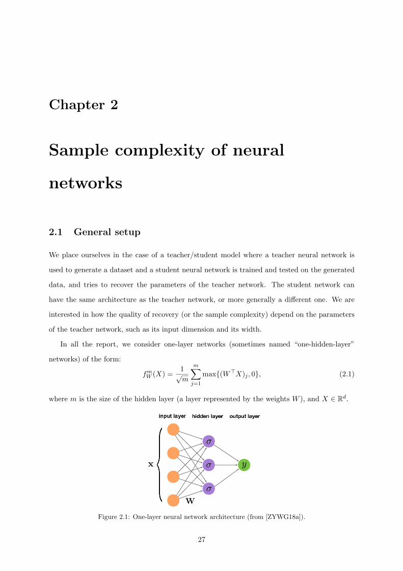
In all the report, we consider one-layer networks (sometimes named “one-hidden-layer”
networks) of the form:
fmW (X) =1√m
m∑j=1
max(W>X)j , 0, (2.1)
where m is the size of the hidden layer (a layer represented by the weights W ), and X ∈ Rd.
Figure 2.1: One-layer neural network architecture (from [ZYWG18a]).
27

CHAPTER 2. SAMPLE COMPLEXITY OF NEURAL NETWORKS
We define Fm = fmW : Rd 7→ R, W ∈ Rd×m the class of such networks.
These networks are initialized using W ∗ ∼ U(− 1√
d, 1√
d
), the uniform distribution between
− 1√d
and 1√d
(called He initialization, introduced in [HZRS15]), so that the variance is stable
through forward propagation in the network.
The empirical loss function we use for model training throughout the report writes, for two
networks fmW ∗ ∈ Fm and fm′
W ∈ Fm′ , and for a dataset of points X1, ..., XN:
LN (fmW ∗ , fm′W ) =
1
N
N∑i=1
1√m
m∑j=1
max(W ∗>Xi)j , 0 −1√m′
m′∑j=1
max(W>Xi)j , 0
2
, (2.2)
The loss used for evaluating the quality of a network output will simply be defined as 1σ2 LN ,
where σ is the empirical standard deviation (where the randomness comes from X) of fmW ∗(X)
(in the following, the weights W ∗ will be fixed, so σ becomes a constant). Remark that, when
W is such that, for all i:
1√m′
m′∑j=1
max(W>Xi)j , 0 =1
N
N∑i=1
1√m
m∑j=1
max(W ∗>Xi)j , 0
, (2.3)
meaning that the output of the student network is constant, then we have:
1
σ2LN (fmW ∗ , f
m′W ) = 1, (2.4)
by definition of the standard deviation of fmW ∗ , which is σ. This means that the loss is maximal
when the student network simply outputs a constant, which is a standard normalization. Hence
using this loss definition for our “quality of recovery” definition is simply appropriately re-scaling
the training loss function.
2.2 Experiments
For given values of N , m and d, we can simulate a random target network fmW ∗ , and use it
to generate two toy datasets of size N , with points x1, ..., xN ∼ N (0, Id) (the d-dimensional
standard normal distribution), and labels y1, ..., yN such that yi = fmW ∗(xi). These two
datasets will be the training and testing sets, generated by what we called earlier the teacher
network.
We check that the standard deviation of the labels does not depend on d, through this
28

CHAPTER 2. SAMPLE COMPLEXITY OF NEURAL NETWORKS
initialization. Indeed, we have:
V[(W>X)i
]= V
d∑j=1
Wj,iXj
=
d∑j=1
V [Wj,i]V [Xj ] ∝d∑j=1
1
d· 1 = 1, (2.5)
using the independence of X and W pre-training, and the unit-scaling of X. Similarly, the
standard deviations of the labels don’t depend on the width m:
V
1√m
m∑j=1
max(W>X)j , 0
∝ 1
m
m∑j=1
V[(W>X)j
]∝ 1 (2.6)
Though not crucial in the analysis, it is always a good practice to keep a normalized scaling for
the output of the network.
For a given target network W ∗, we define for simplicity of notation LN (W ) = LN (fmW ∗ , fm′W ).
We will fix in the following m′ = m (the learner network has the same architecture as the teacher
network), hence we can drop the subscript. If we further define the labels (Yi)Ni=1 as the forward
passes of the X’s through the target network, then we get:
LN (W ) =
N∑i=1
Yi − 1
m
m∑j=1
max(W>Xi)j , 0
2
. (2.7)
The loss of course implicitly depends on W ∗ through these labels.
Notice that the choice of evaluating the recovery performance using 1σ2 L is not innocent. In
fact, recall that, in the standard case of a model:
Y = f(X) + ε, (2.8)
then the coefficient of determination of the model, or R2, is given by, where Y is our estimate
of Y and Y the average value of Y :
1−R2 =
1N
∑Ni=1
(Yi − Yi
)21N
∑Ni=1
(Yi − Y
)2 ∼ 1
σ2· L (2.9)
Hence our measure of error is similar to(1−R2
), and we can threshold it by a value between
0 and 1, depending on how precise we want the recovery to be. Note that if our estimate of the
true network is a constant equal to the expectation of this network, our loss measure will return
29
CHAPTER 2. SAMPLE COMPLEXITY OF NEURAL NETWORKS
a value of 1, which would give an R2 of 0 according to this formula. This is indeed what we
want, and what is usual in statistics: a linear model fitting only the mean of a dataset should
be assigned a performance of 0 out-of-sample.
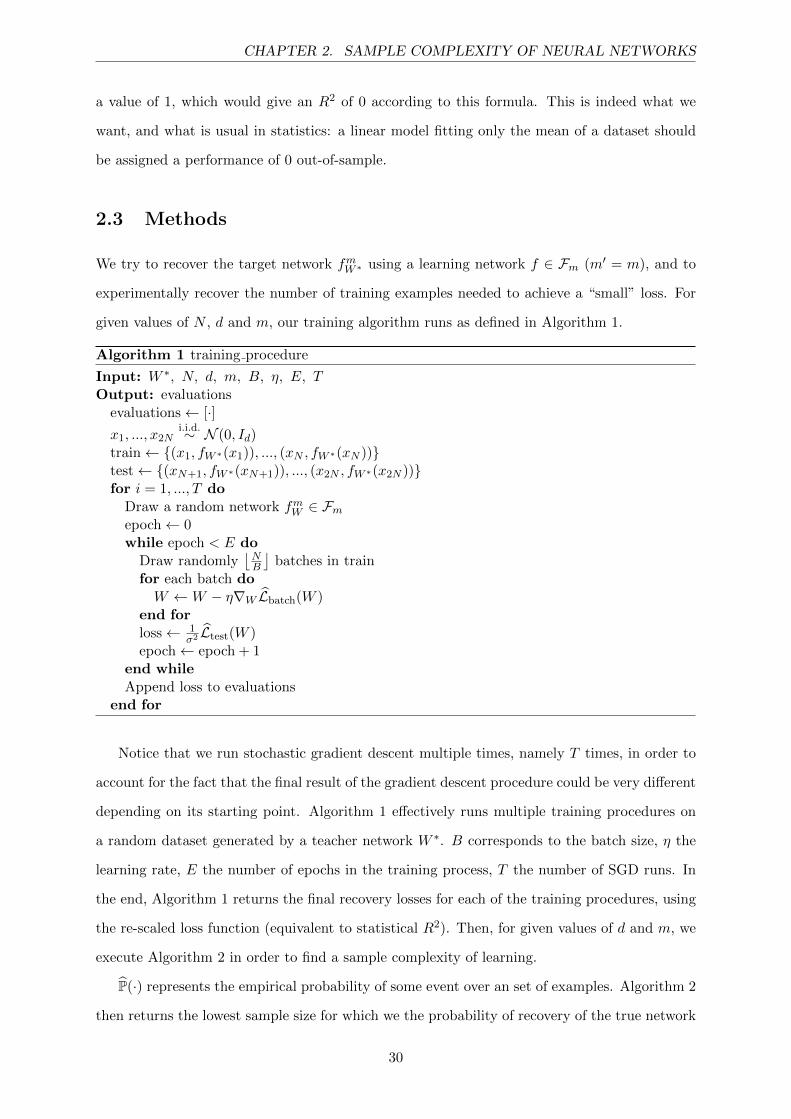
2.3 Methods
We try to recover the target network fmW ∗ using a learning network f ∈ Fm (m′ = m), and to
experimentally recover the number of training examples needed to achieve a “small” loss. For
given values of N , d and m, our training algorithm runs as defined in Algorithm 1.
Algorithm 1 training procedure
Input: W ∗, N, d, m, B, η, E, TOutput: evaluations
evaluations← [·]x1, ..., x2N
i.i.d.∼ N (0, Id)train← (x1, fW ∗(x1)), ..., (xN , fW ∗(xN ))test← (xN+1, fW ∗(xN+1)), ..., (x2N , fW ∗(x2N ))for i = 1, ..., T do
Draw a random network fmW ∈ Fmepoch← 0while epoch < E do
Draw randomly⌊NB
⌋batches in train
for each batch doW ←W − η∇W Lbatch(W )
end forloss← 1
σ2 Ltest(W )epoch← epoch + 1
end whileAppend loss to evaluations
end for
Notice that we run stochastic gradient descent multiple times, namely T times, in order to
account for the fact that the final result of the gradient descent procedure could be very different
depending on its starting point. Algorithm 1 effectively runs multiple training procedures on
a random dataset generated by a teacher network W ∗. B corresponds to the batch size, η the
learning rate, E the number of epochs in the training process, T the number of SGD runs. In
the end, Algorithm 1 returns the final recovery losses for each of the training procedures, using
the re-scaled loss function (equivalent to statistical R2). Then, for given values of d and m, we
execute Algorithm 2 in order to find a sample complexity of learning.
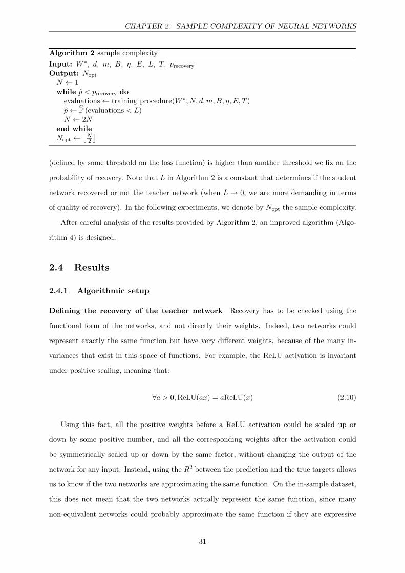
P(·) represents the empirical probability of some event over an set of examples. Algorithm 2
then returns the lowest sample size for which we the probability of recovery of the true network
30
CHAPTER 2. SAMPLE COMPLEXITY OF NEURAL NETWORKS
Algorithm 2 sample complexity
Input: W ∗, d, m, B, η, E, L, T, precoveryOutput: Nopt
N ← 1while p < precovery do
evaluations← training procedure(W ∗, N, d,m,B, η,E, T )p← P (evaluations < L)N ← 2N
end whileNopt ←
⌊N2
⌋(defined by some threshold on the loss function) is higher than another threshold we fix on the
probability of recovery. Note that L in Algorithm 2 is a constant that determines if the student
network recovered or not the teacher network (when L → 0, we are more demanding in terms
of quality of recovery). In the following experiments, we denote by Nopt the sample complexity.
After careful analysis of the results provided by Algorithm 2, an improved algorithm (Algo-
rithm 4) is designed.
2.4 Results
2.4.1 Algorithmic setup
Defining the recovery of the teacher network Recovery has to be checked using the
functional form of the networks, and not directly their weights. Indeed, two networks could
represent exactly the same function but have very different weights, because of the many in-
variances that exist in this space of functions. For example, the ReLU activation is invariant
under positive scaling, meaning that:
∀a > 0,ReLU(ax) = aReLU(x) (2.10)
Using this fact, all the positive weights before a ReLU activation could be scaled up or
down by some positive number, and all the corresponding weights after the activation could
be symmetrically scaled up or down by the same factor, without changing the output of the
network for any input. Instead, using the R2 between the prediction and the true targets allows
us to know if the two networks are approximating the same function. On the in-sample dataset,
this does not mean that the two networks actually represent the same function, since many
non-equivalent networks could probably approximate the same function if they are expressive
31

CHAPTER 2. SAMPLE COMPLEXITY OF NEURAL NETWORKS
enough. However, checking the R2 between the prediction and the true targets on the out-of-
sample set allows us to know if those two functions are the same, which is the best we can do
to objectively decide if recovery of the teacher network happened or not.
Parameters For all the experiments, we used Algorithm 1 with full gradient descent, namely
B = N , a learning rate of η = 5× 10⁻³, a maximum number of epochs E = 300, and T = 100
iterations of gradient descent for every dataset.
For the sample complexity experiments, the threshold on the probability of recovery is fixed
to precovery = 0.5. The threshold on the quality of recovery is fixed to L = 0.95. Namely, a
student network is defined to be successful in the recovery of the teacher network if its out-
of-sample R2 is at least 95%. A set of different student networks is defined to have achieved
“global” recovery of a teacher network if at least half of them achieved it.
Because we study the dependence of the sample complexity on d and m, the scaling of the
parameters L and precovery in Algorithm 2 doesn’t matter much. It just re-scales the sample
complexity without changing its dependence on d or m (of course, if the level of recovery we
want to achieve increases, namely L decreases, the sample complexity will be higher). What
matters is that those parameters are the same for different values of d and m.
This set of values allows algorithms to scale much better when facing the noise of the
experiments. In particular, a value of precovery closer to 1 would make more sense, but our
experiments showed that the time scaling of Algorithm 2 was very bad in precovery. This is
explained by the fact that, even if the dataset is bigger than the required sample complexity,
some of the SGD training processes will still fail to recover the global optimum, simply because
this procedure is not guaranteed to converge on such non-convex objectives. Allowing a portion
of those training procedures to fail scales the algorithms on the order of hours instead of days.
2.4.2 Recovery precision
First, we use a slight modification of Algorithm 2 (Algorithm 3), which only looks at the quality
of the approximation of the teacher network by the student network, without defining the notion
of whether the student network was able to recover the teacher network or not.
E[1−evaluations] represents the empirical average of the out-of-sample R2 (obtained through
the re-scaled loss function) across all the training procedures. Instead of directly looking at the
sample complexity, which requires us to define some arbitrary criterion regarding whether the
32
CHAPTER 2. SAMPLE COMPLEXITY OF NEURAL NETWORKS
Algorithm 3 recovery r2
Input: W ∗, d, m, B, η, E, TOutput: R2
recovery
evaluations← training procedure(W ∗, N, d,m,B, η,E, T )R2
recovery ← E[1− evaluations]
recovery of the target network happened or not (namely L in Algorithm 2), we instead consider
the average recovery quality, and see how this “recovery quality” behaves as a function of
network parameters. This enables us to examine the impact of the three main variables – the
input dimension d, the hidden dimension m, and the sample size N – on the difficulty of the
recovery task. By displaying the average recovery R2 as a function of these variables, for varying
values of a second variable of importance, we can clearly see how these three variables impact
the difficulty of the recovery task presented here. This provides insight as to how training neural
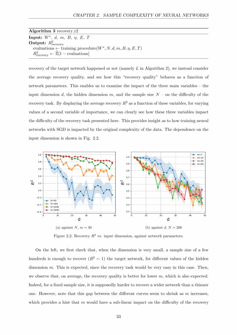
networks with SGD is impacted by the original complexity of the data. The dependence on the
input dimension is shown in Fig. 2.2.
(a) against N , m = 30 (b) against d, N = 200
Figure 2.2: Recovery R2 vs. input dimension, against network parameters.
On the left, we first check that, when the dimension is very small, a sample size of a few
hundreds is enough to recover (R2 ∼ 1) the target network, for different values of the hidden
dimension m. This is expected, since the recovery task would be very easy in this case. Then,
we observe that, on average, the recovery quality is better for lower m, which is also expected.
Indeed, for a fixed sample size, it is supposedly harder to recover a wider network than a thinner
one. However, note that this gap between the different curves seem to shrink as m increases,
which provides a hint that m would have a sub-linear impact on the difficulty of the recovery
33

CHAPTER 2. SAMPLE COMPLEXITY OF NEURAL NETWORKS
task. For a fixed hidden dimension, the recovery task becomes extremely hard if d becomes too
large, but is quite easy for small d, even for relatively small dataset sizes (N = 50 for example
is enough to have a good recovery quality for very low input dimensions). In both sub-figures,
we also observe that the recovery quality decreases at a close-to-linear rate as a function of the
input dimension d.
The dependence of the average recovery R2 on the hidden dimension m is shown in Fig. 2.3.
(a) against N , d = 30 (b) against d, N = 500
Figure 2.3: Recovery R2 vs. hidden dimension, against network parameters.
This time, the conclusions are quite different. Of course, the recovery task is still more
difficult for higher m and higher d. However, we also see that the gap between the different
curves (for different input dimensions d) does not seem to shrink as the input dimension grows.
Similarly, the decay of the recovery R2 as a function of the hidden dimension m seems to be sub-
linear, as we guessed with Fig. 2.2. For m large enough, the average recovery R2 stabilizes. We
also see that m almost doesn’t impact the recovery R2 above a certain threshold, for different
dataset sizes.
Finally, looking at the recovery quality as a function of the sample size shows how many
samples are needed to properly recover the target network, which gives a good idea of the
magnitude of the empirical sample complexity, as we will study below.
Those results are shown in Fig. 2.4. In both cases, the quality of the recovery of the target
network grows at a seemingly at least polynomial rate when growing the dataset size. Again, we
observe that the gap between the curves for different input dimensions is quite stable, whereas
this gap shrinks when growing the hidden dimension instead.
34

CHAPTER 2. SAMPLE COMPLEXITY OF NEURAL NETWORKS
(a) against m, d = 30 (b) against d, m = 30
Figure 2.4: Recovery R2 vs. sample size, against network parameters.
2.4.3 Sample complexity
When studying the dependence of the sample complexity on d, we fix m = 5. Similarly, when
studying the dependence of the sample complexity on m, we fix d = 5. This choice of relatively
small parameters is dictated by the computationally-heavy nature of those experiments, which
in general take on the order of tens of hours to run. This is due to the fact that the algorithms
presented above contain many nested loops, which are needed in order to eliminate the noise in
the experiments by as much as we can.
A first un-satisfactory approach
The dependence of the sample complexity on the input dimension obtained with Algorithm 2
is shown in Fig. 2.5.
Figure 2.5: Sample complexity vs. input dimension and best linear fits, without dichotomy.
35

CHAPTER 2. SAMPLE COMPLEXITY OF NEURAL NETWORKS
We also fit different parametrized models (polynomial, logarithmic-polynomial, and loga-
rithmic) on the curve obtained, and plot them in Fig. 2.5. Their forms with the corresponding
R2 are as follows: Nopt ∝ A · d1.1 R2 = 0.913
Nopt ∝ B · d0.7 log d R2 = 0.921
Nopt ∝ C · (log d)2.5 R2 = 0.901
(2.11)
The dependence on d is clearly positive, but the different parametrizations do not have a
perfectly satisfactory quality, as measured by their R2, or as seen on Fig. 2.5. One can see that
very different fits, such as O((log d)2.5) and O(d1.1), have similar scores, which in turn doesn’t
enable us to really establish the dependence of the sample complexity on the input dimension.
Because we can’t scale to very large input dimensions, we also lack a sufficient number of points
in order to eliminate the noise seen in Fig. 2.5, which seemingly makes sample complexity drop
sometimes, even when growing d (as seen on some points in the right part of the graph).
The dependence on m is even less clear, as shown in Fig. 2.6.
Figure 2.6: Sample complexity vs. hidden dimension and best linear fits, without dichotomy.
The corresponding parametrized fits are as follows:
Nopt ∝ A′ ·m−0.4 R2 = 0.114
Nopt ∝ B′ ·m−1.5(logm)3 R2 = 0.184
Nopt ∝ C ′ · (logm)−0.7 R2 = 0.068
(2.12)
With this approach, the fits can’t capture the effect of m, and it even seems that m doesn’t
quite have any impact on the sample complexity. The obtained points in blue are overall very
36
CHAPTER 2. SAMPLE COMPLEXITY OF NEURAL NETWORKS
noisy, and it is quite challenging to obtain any statistically significant relationship from this
result.
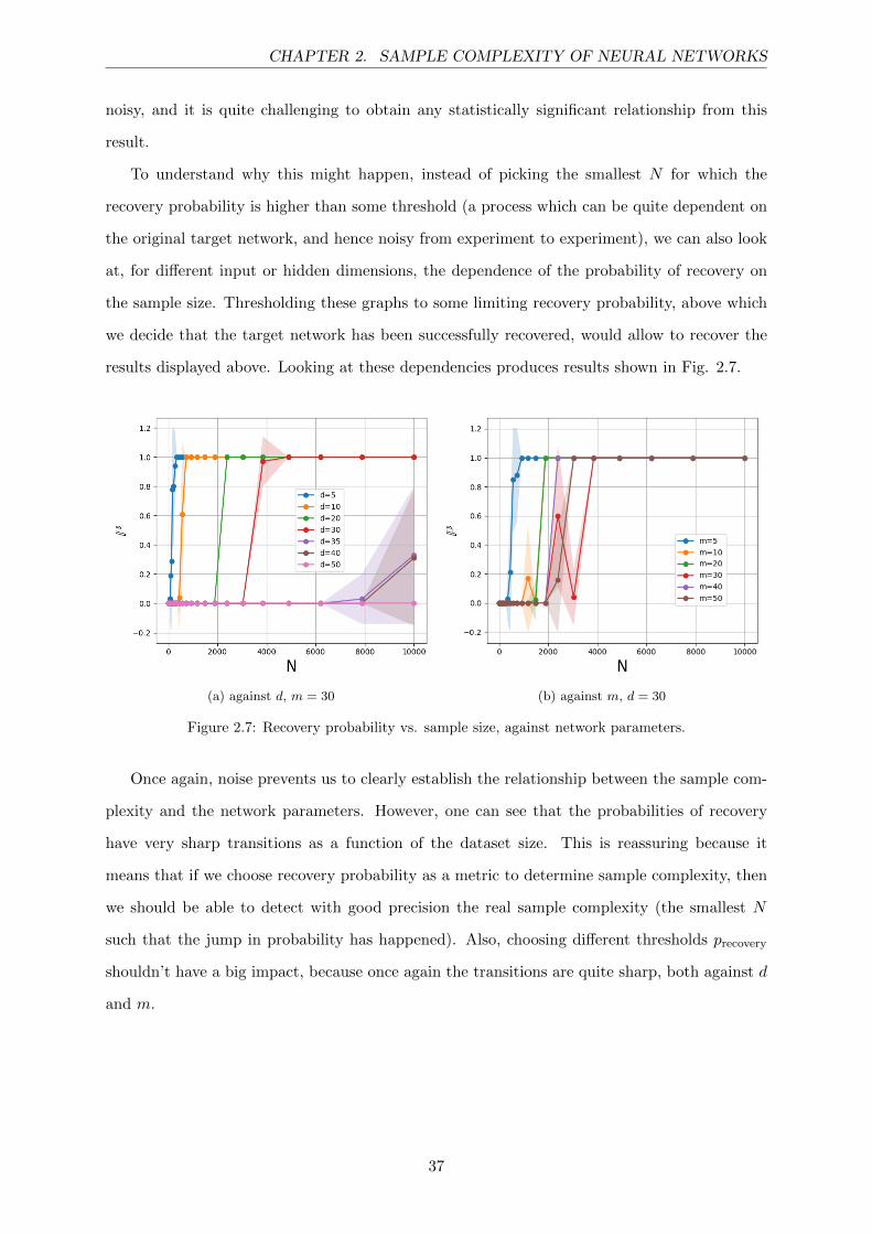
To understand why this might happen, instead of picking the smallest N for which the
recovery probability is higher than some threshold (a process which can be quite dependent on
the original target network, and hence noisy from experiment to experiment), we can also look
at, for different input or hidden dimensions, the dependence of the probability of recovery on
the sample size. Thresholding these graphs to some limiting recovery probability, above which
we decide that the target network has been successfully recovered, would allow to recover the
results displayed above. Looking at these dependencies produces results shown in Fig. 2.7.
(a) against d, m = 30 (b) against m, d = 30
Figure 2.7: Recovery probability vs. sample size, against network parameters.
Once again, noise prevents us to clearly establish the relationship between the sample com-
plexity and the network parameters. However, one can see that the probabilities of recovery
have very sharp transitions as a function of the dataset size. This is reassuring because it
means that if we choose recovery probability as a metric to determine sample complexity, then
we should be able to detect with good precision the real sample complexity (the smallest N
such that the jump in probability has happened). Also, choosing different thresholds precovery
shouldn’t have a big impact, because once again the transitions are quite sharp, both against d
and m.
37

CHAPTER 2. SAMPLE COMPLEXITY OF NEURAL NETWORKS
Computational issues and improvements
The sample complexity results obtained using Algorithm 2 are not very satisfying for multiple
reasons:
• The shapes of the sample complexity curves seem to be too noisy from experiment to
experiment (especially, hugely dependent on the target network used for each d or m).
• The empirical sample complexity curves display jumps of a factor 2, because the sample
complexity found using Algorithm 2 is multiplied or divided by 2.
• We are not able to fit a satisfying simple relationship between the empirical complexity,
and the input or hidden dimension.
Having to jump from N to 2N at each step in Algorithm 2 creates the second and third issues.
The second one is more problematic. It is due to the procedure introduced in Algorithm 2 that
creates an exponential spacing between the different possible sample complexities that we might
obtain. To remedy this problem, we design a variant of Algorithm 2, Algorithm 4.
Algorithm 4 sample complexity dichotomy
Input: W ∗, d,m,B, η,E, L, T, precovery, depthOutput: Nopt
Nhigh ← sample complexity(W ∗, d, m, B, η, E, L, T, precovery)
Nlow ←⌊Nlow2
⌋for i = 1, ...,depth do
N ←⌊Nlow+Nhigh
2
⌋evaluations← training procedure(W ∗, N, d,m,B, η,E, L, T )p← P (evaluations < L)if p < precovery thenNlow ← N
elseNhigh ← N
end ifend forNopt ← Nhigh
This algorithm, after obtaining the final upper bound on the sample complexity, runs a
backwards dichotomy procedure to find a more precise estimation of the true sample complexity
between the original Nopt andNopt
2 . The dichotomy procedure is ran for some pre-specified depth
(here 4, which reduces the “jump” size in the empirical sample complexity by 24 = 16), to avoid
losing too much computational efficiency while still gaining much in terms of precision.
38

CHAPTER 2. SAMPLE COMPLEXITY OF NEURAL NETWORKS
Moreover, in order to reduce the noise in the experiments due to the choice of a particular
target network for each dimension d or hidden layer size m, we decide to run 10 independent
parallel computations, and average the empirical sample complexities found for each of the 10
target networks. For a fixed d or m, each of those computations operates on a different target
network, which averages out the noise in the empirical sample complexity found for each single
target network.
The results obtained using Algorithm 4 are much more satisfactory and can be seen in Fig.
2.8, for the dependence on m.
(a) various trials (different target networks) (b) median trial
Figure 2.8: Sample complexity trials vs. hidden dimension, with dichotomy.
The figure on the left shows the dependence of the sample complexity on log(m) across
the 10 different trials operating on different target networks. It is now clear that the previous
approach was suffering from running the experiment only once. Indeed, we see in the figure on
the left that the empirical sample complexity of the network is highly randomized around its
“true” value (because, for each curve, the target network is fixed and might have properties that
make it easier or more difficult to recover). For the same hidden dimension, empirical sample
complexities can extend or shrink by a factor at least 2, according to the experiments. In very
rare cases, it can even drop more than usual, because of the randomness in the choice of the
target network.
Taking the median of the empirical sample complexities across trials yields much cleaner
curves, as shown in the right plot of Fig. 2.8. We choose the median instead of the average
to be more robust to the many outliers that we observed in the left part of the figure, across
39
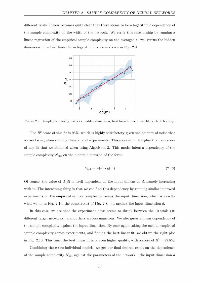
CHAPTER 2. SAMPLE COMPLEXITY OF NEURAL NETWORKS
different trials. It now becomes quite clear that there seems to be a logarithmic dependency of
the sample complexity on the width of the network. We verify this relationship by running a
linear regression of the empirical sample complexity on the averaged curve, versus the hidden
dimension. The best linear fit in logarithmic scale is shown in Fig. 2.9.
Figure 2.9: Sample complexity trials vs. hidden dimension, best logarithmic linear fit, with dichotomy.
The R2 score of this fit is 95%, which is highly satisfactory given the amount of noise that
we are facing when running these kind of experiments. This score is much higher than any score
of any fit that we obtained when using Algorithm 2. This model infers a dependency of the
sample complexity Nopt on the hidden dimension of the form:
Nopt ∼ A(d) log(m) (2.13)
Of course, the value of A(d) is itself dependent on the input dimension d, namely increasing
with it. The interesting thing is that we can find this dependency by running similar improved
experiments on the empirical sample complexity versus the input dimension, which is exactly
what we do in Fig. 2.10, the counterpart of Fig. 2.8, but against the input dimension d.
In this case, we see that the experiment noise seems to shrink between the 10 trials (10
different target networks), and outliers are less numerous. We also guess a linear dependency of
the sample complexity against the input dimension. By once again taking the median empirical
sample complexity across experiments, and finding the best linear fit, we obtain the right plot
in Fig. 2.10. This time, the best linear fit is of even higher quality, with a score of R2 = 99.8%.
Combining those two individual models, we get our final desired result on the dependence
of the sample complexity Nopt against the parameters of the network – the input dimension d
40

CHAPTER 2. SAMPLE COMPLEXITY OF NEURAL NETWORKS
(a) various trials (different target networks) (b) median trial and best linear fit
Figure 2.10: Sample complexity vs. input dimension, trials and best linear fit, with dichotomy.
and the hidden dimension m:
Nopt ∼ d · log(m) (2.14)
This result is quite remarkable, for different reasons:
• The dependence on d is linear, which goes against the existing belief that the sample
complexity should be a higher order polynomial of the data dimension.
• The logarithmic dependence on m can provide the start of an answer to a commonly
observed phenomenon in deep learning, namely that over-parametrizing neural networks
doesn’t hurt their performance. Our experiments show that, even when over-parametrizing
the network in width, the number of training examples needed to achieve good out-
of-sample performance grows very slowly with the width. Hence, one can extend the
network’s width exponentially while only having to grow the dataset size linearly.
• The overall dependence of the sample complexity on network parameters shows that neural
networks can in practice find very good local optima without having to be fed as many
data points as standard statistical knowledge would say.
Overall, we consider those empirical facts as a very strong hint towards understanding why
neural networks achieve very good performance even when over-parametrizing them by orders
of magnitude larger compared to the dataset sizes at hand.
41

THIS PAGE INTENTIONALLY LEFT BLANK
42
Chapter 3
Polynomial regression
3.1 General setup
We now introduce polynomial regression as a way to approximate neural networks while preserv-
ing their good performance, and adding interpretability of features and convergence guarantees
of the training process on top of this. Recall that a one-layer (of width m) neural network with
activation f writes (in the first chapter, we chose bi = 1√m
constant):
Y =
m∑i=1
bif([W>X]i) (3.1)
Now assume that f is polynomial of degree k, namely that there exists a0, ..., ak such that:
f(x) = a0 + a1x+ ...+ akxk (3.2)
Then we can re-write the output of the network as:
Y =m∑i=1
bi
a0 + a1
d∑j=1
Wj,iXj
+ ...+ ak
d∑j=1
Wj,iXj
k (3.3)
This in turns re-writes as:
Y =
k∑t=1
∑α∈Nd∑di=1 αi=t
W (t)α1,...,αd
Xα11 ...Xαd
d (3.4)
43

CHAPTER 3. POLYNOMIAL REGRESSION
where W(t)α1,...,αd = at
∑mi=1 biW
α11,i ...W
αdd,i . In all the following, we call k the “tensor degree”. For
example, we have: W (0) = a0
∑mi=1 bi
W(1)j = a1
∑mi=1 biWj,i
W(2)j,k = a2
∑mi=1 biWj,iWk,i
(3.5)
where we slightly modify notation, by saying that:
W (0) = W
(0)0,...,0
W(1)j = W
(1)0,...,1,...,0
W(2)j,k = W
(2)0,...,1,...,1,...,0
(3.6)
where the ones are at the jth position for W (1) and the jth and kth positions for W (2).
This formulation leads to several interesting conclusions, that are at the core of the intro-
duction of polynomial regression:
• it shows that Y is a linear combination, with tensor weights W(t)α1,...,αd , of tensor products
Xα11 ...Xαd
d . Said otherwise, the neural network is itself a linear model in the lifted space
of tensor product features.
• this space of tensor products is, if the tensor degree k > 1, of much higher dimension than
the original data dimension d.
• in the space of tensor products, the neural network is a convex function, and it is even
linear. Hence, training on the tensor weights W has the same convergence guarantees as
standard linear regression.
A polynomial regression model is trained using a standard least squares procedure, with the
equation Eq. 3.4, optimizing over the weights W .
Now, we know that if the weights of the network W are initialized properly (namely, to
make sure that the order of magnitude of∑d
j=1Wj,iXj stays O(1)), then the inputs [W>X]i
to the activation function will be O(1). Hence, under some regularity conditions on f , we can
approximate f by a polynomial of some degree over some compact set [−a, a], with a large
enough so that it contains all the inputs [W>X]i with high probability. In turn, we can expect
that the output of any such network (with the original activation function f) will be close
44
CHAPTER 3. POLYNOMIAL REGRESSION
in norm to the one obtained by the same network using the approximating polynomial of f .
Typically, if f is easily approximated by polynomials, we would hope that the output of those
two networks (the one with f , and the one with the polynomial approximation of f) become
very similar. Typically, ReLU activations are used nowadays in deep learning neural networks.
Approximating the ReLU function – over say [−3, 3] – by polynomials, should not be too difficult
of a task, and we hence hope that polynomial regression will be able to display similar good
performance as the one of non-linear multi-layer neural networks using the ReLU activation.
Of course, as the tensor degree grows towards infinity, polynomial regression should be able to
achieve perfect recovery of the initial teacher network, with some regularity conditions on the
activation function f of the teacher network. The main questions are:
• can we scale polynomial regression to high tensor degrees and large datasets?
• how large does the tensor degree k need to be in order to have good performance?
In the following, we focus on those two questions, and study the performance of polynomial
regression on synthetic and real data. We design algorithms that allow scalability and good
performance of the method at the same time.
3.2 Testing on synthetic data
3.2.1 Construction of the synthetic dataset
Our goal here is to take the point of view with which polynomial regression was designed.
Namely, that for polynomial neural networks (neural networks with an activation function that
is polynomial), unwrapping the function computed by the network provides the polynomial
regression formulation, which is a linear combination of tensor products. By definition, poly-
nomial regression can match perfectly the function produced by a polynomial neural network.
Here, we instead look into neural networks with more general activation functions, and see what
behavior polynomial regression exhibits in such cases.
Given a network activation function that can either be the sigmoid function f(x) = 11+e−x or
the ReLU function f(x) = max(x, 0), we draw random i.i.d. weights according to the Gaussian
distribution N (0, 1). For a given input dimension d and hidden dimension m, we draw dm of
those weights. We denote this d ×m matrix of weights W . As expected, xW will provide the
output of the hidden layer of the network before applying the activation function. Since we will
45

CHAPTER 3. POLYNOMIAL REGRESSION
use the polynomial regression method in the area of image recognition, we choose to make the
matrix W sparse such that, for each hidden unit in the hidden layer W , this unit only multiplies
at most s of the input vector coordinates (in a contiguous way). This makes the neural network
effectively operate like a CNN on the input data. Having chosen those various parameters, we
then draw N random Bernoulli variables of dimension d (and re-normalize them to −1, 1),
which will form the input dataset X. The targets of the synthetic dataset are obtained by
pushing X through the network using Eq. 3.1, with identical bi for all i = 1, ...,m.
This provides us with an (X,Y ) dataset generated by a neural network in a convolutional
way. Finally, we fit a polynomial regression model (by optimizing a standard least squares
objective) to this dataset, by choosing various degrees for the tensor products (namely 1, 2, 3
and 4). We vary d, m, N , and the activation function as well. With the limited resources of
a personal computer, we only experiment up to d ∼ 25 and s ∼ 16, for degree k = 4 tensor
products, for which the number of tensor products is already of order hundreds of thousands.
Experimenting on synthetic datasets allows to control the data dimension, which in turn makes
polynomial regression fully tractable for higher tensor degrees (compared to the degrees we can
use on real data).
3.2.2 Impact of d and m
We empirically recover the fact that for m large enough, the performance of polynomial regres-
sion does not depend (or depends very loosely) on m. We show in Fig. 3.1 the dependence of
the out-of-sample R2 against m, for d = 20, with a ReLU activation, and with a tensor degree
equal to 2. The number of samples is n = 2,000. Choosing the sigmoid activation or a higher
tensor degree does not change the fact that the curve does not vary with m, on average. Of
course there is a lot of noise involved in these experiments, since we have to re-generate the
dataset (because the teacher network is itself re-generated) for each value of m, which in turn
might yield easier-to-learn or more challenging datasets, depending on the random draw. The
sparsity parameter s is chosen as the minimum between d and 9.
Fig. 3.1 confirms the results of the previous section for which we found that the dependence
on m was very loose after a certain threshold. Similarly, when the input dimension d varies, the
performance shrinks linearly with d before hitting its minimum. These results are consistent
with the empirical findings of the previous chapter, with a linear drop of the out-of-sample
performance as a function of d.
46

CHAPTER 3. POLYNOMIAL REGRESSION
(a) vs. d, m = 20 (b) vs. m, d = 20
Figure 3.1: Performance of polynomial regression for synthetic datasets vs. network parameters.
3.2.3 Sample complexity
Now, we turn to the sample complexity measure, namely the dataset size for which the gener-
alization gap (the difference between the in-sample and out-of-sample R2) is small. Of course,
this gap depends on many of the parameters introduced here, like d or m, typically. However,
we can look at the ratio of the sample size to the number of polynomial regression features
(denoted p here) versus the in-sample/out-of-sample performance gap. In distribution, we see
in Fig. 3.2 that the accuracy gap presents an inflection point around N/p = O(1), which would
clue us into the fact that one would only need approximately as many training examples as
polynomial tensor products p. Even if this is for now a wild guess, we will see in the following
sections while doing experiments on real data that it actually holds in practice, and makes
polynomial regression more practical.
Figure 3.2: Generalization gap vs. ratio of dataset size to number of polynomial regression features.
47
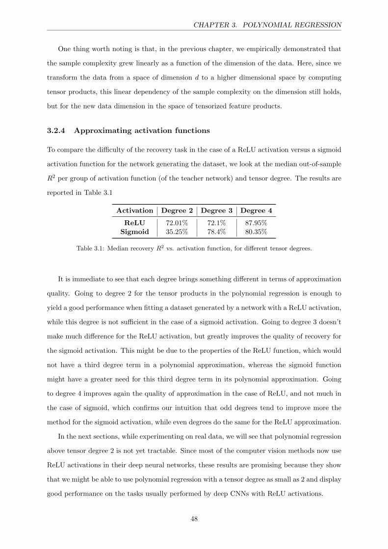
CHAPTER 3. POLYNOMIAL REGRESSION
One thing worth noting is that, in the previous chapter, we empirically demonstrated that
the sample complexity grew linearly as a function of the dimension of the data. Here, since we
transform the data from a space of dimension d to a higher dimensional space by computing
tensor products, this linear dependency of the sample complexity on the dimension still holds,
but for the new data dimension in the space of tensorized feature products.
3.2.4 Approximating activation functions
To compare the difficulty of the recovery task in the case of a ReLU activation versus a sigmoid
activation function for the network generating the dataset, we look at the median out-of-sample
R2 per group of activation function (of the teacher network) and tensor degree. The results are
reported in Table 3.1
Activation Degree 2 Degree 3 Degree 4
ReLU 72.01% 72.1% 87.95%Sigmoid 35.25% 78.4% 80.35%
Table 3.1: Median recovery R2 vs. activation function, for different tensor degrees.
It is immediate to see that each degree brings something different in terms of approximation
quality. Going to degree 2 for the tensor products in the polynomial regression is enough to
yield a good performance when fitting a dataset generated by a network with a ReLU activation,
while this degree is not sufficient in the case of a sigmoid activation. Going to degree 3 doesn’t
make much difference for the ReLU activation, but greatly improves the quality of recovery for
the sigmoid activation. This might be due to the properties of the ReLU function, which would
not have a third degree term in a polynomial approximation, whereas the sigmoid function
might have a greater need for this third degree term in its polynomial approximation. Going
to degree 4 improves again the quality of approximation in the case of ReLU, and not much in
the case of sigmoid, which confirms our intuition that odd degrees tend to improve more the
method for the sigmoid activation, while even degrees do the same for the ReLU approximation.
In the next sections, while experimenting on real data, we will see that polynomial regression
above tensor degree 2 is not yet tractable. Since most of the computer vision methods now use
ReLU activations in their deep neural networks, these results are promising because they show
that we might be able to use polynomial regression with a tensor degree as small as 2 and display
good performance on the tasks usually performed by deep CNNs with ReLU activations.
48

CHAPTER 3. POLYNOMIAL REGRESSION
3.3 Testing on real data – setup and benchmarks
3.3.1 Setup
We implemented our polynomial regression method on the MNIST [LeC98] and Fashion-MNIST
[XRV17] datasets, both of which are predominantly approached using neural networks and
serve as widely used testbeds for deep learning algorithms. Both datasets contains N = 60,000
training images, each consisting of 28 × 28 gray-scale pixels, that is, a dimension of d = 784.
We study both datasets as a classification task with 10 classes. Their corresponding test sets
contain 10,000 images. Because of the computational cost of polynomial regression, we are for
now limited to such datasets for which the number of pixels per image is not of order higher than
thousands. For MNIST, the 10 classes are the ten digits from 0 to 10, and an example image
is shown in Fig. 3.3. For Fashion-MNIST, the 10 classes represent different types of clothing,
namely: t-shirt, trouser, pullover, dress, coat, sandal, shirt, sneaker, bag or ankle boot. It is
commonly accepted and seen in practice that the classification task on Fashion-MNIST is harder
than the one on MNIST, as shown below by the state-of-the-art accuracies on both datasets.
(a) MNIST (b) Fashion-MNIST
Figure 3.3: Example images from datasets used.
3.3.2 State-of-the-art models
During this study we will be using several benchmarks to compare the performance of our
polynomial regression method with that of existing models, either in the literature, or that
we create ourselves. To have a first idea of how the best-performing models in the literature
behave on those datasets, we can report the accuracy of some recent state-of-the-art models. On
MNIST, [WZZ+13] reports state-of-the-art out-of-sample accuracy, while for Fashion-MNIST,
[ZZK+17] does. We report those accuracy values in Table 3.2.
49

CHAPTER 3. POLYNOMIAL REGRESSION
Dataset Accuracy
MNIST 99.79%Fashion-MNIST 96.35%
Table 3.2: Out-of-sample accuracy of state-of-the-art models.
Remark It is important to understand that those state-of-the-art models were obtained using
much more complex infrastructure and much longer computation time than any of the ones we
implemented. Typically, those models contain on order millions of parameters (compared to
roughly twenty thousand parameters for polynomial regression on MNIST and Fashion-MNIST,
as shown in the next sections), and are trained on highly optimized clusters of GPUs or TPUs
for computer-times of many days or months (the parallelization times the time spent on training
for each sub-process). We hence did not have at any point any hope of improving the state-of-
the-art models in terms of pure accuracy. We are rather aiming at introducing a new method
that displays several advantages that might be of very important use in applications where
accuracy is not the only thing that matters. For example, interpretability might be a critical
factor in medical or justice applications. One might even argue that some of the computer vision
applications, which we focus on here, should give more importance to interpretability, in order
to analyze a posteriori why a system chose an action that it chose to take. Other advantages,
which we will develop further below, include robustness, as well as more convergence guarantees
during the training process.
3.3.3 A deep learning inspired approach
In order to develop a more fair comparison between our polynomial regression method and
existing deep learning methods that are typically used on computer vision tasks, we designed
standard deep learning models of comparable size to the polynomial regression model presented
below, and also trained them for a similar computer-time.
We implemented a CNN model with 2 layers. Each layer is composed of a convolution, a
ReLU activation, and a batch normalization (a layer that learns the normalization of the data).
Then, there are two final fully connected layers that transform the data to dimension 10 for
prediction. The predicted class is then chosen according to the arg max of the output vector,
as is common practice. This is a standard architecture for document recognition, inspired from
the one of a widely used network for such tasks, namely LeNet-5 [LBBH98]. This network’s
50

CHAPTER 3. POLYNOMIAL REGRESSION
architecture is shown in Fig. 3.4.
Figure 3.4: LeNet5 architecture.
Our version is a very similar, and simplified version of this architecture. More precisely, the
architecture we use is as follows (the stride being the minimum filter movements):
• a convolutional filter of size 5 × 5, with 32 output channels, stride 1 and padding 2, a
ReLU activation and a max-pool operation of size 2× 2 and stride 2.
• a convolutional filter of size 5 × 5, with 64 output channels, stride 1 and padding 2, a
ReLU activation and a max-pool operation of size 2× 2 and stride 2.
• a dropout layer, a fully-connected layer with 1,000 outputs and a fully-connected layer
with 10 outputs (the final layer).
This architecture was trained for a similar amount of time (around 30 minutes) as our
polynomial regression model, using SGD for 10 epochs with batches of size 100. Making those
hyper-parameters vary didn’t change the accuracy much, and it is checked a posteriori that the
out-of-sample accuracy has been plateauing for many epochs at the end of the training process.
The out-of-sample accuracy during the training process against the number of batches seen
(each batch being of size 100) is shown on Fig. 3.5. By looking at the scale on the left of the
graphs, we see that the out-of-sample accuracy converged very quickly to its limit.
The final out-of-sample accuracies of the two models are shown in Table 3.3 (they differ
slightly from the last points on the graphs, because we only recorded the out-of-sample accuracy
during the training process once every 50 batches, not for every batch).
Those will be the points of comparison when measuring the quality of polynomial regres-
sion against deep learning models. Again, if we were able to run more large-scale polynomial
regression than what shown below, we would compare it to more complex networks trained for
longer. The point is that, for the networks trained here, the comparison is fair.
51

CHAPTER 3. POLYNOMIAL REGRESSION
(a) MNIST (b) Fashion-MNIST
Figure 3.5: Out-of-sample accuracy of the CNN model during the training process, zoomed.
Dataset Accuracy
MNIST 99.03%Fashion-MNIST 90.80%
Table 3.3: Out-of-sample accuracy of CNN models after training.
3.3.4 A dimensionality reduction approach
Even if the size of the MNIST and Fashion-MNIST images is only 784 pixels, polynomial
regression remains intractable for tensor degrees of 2 or higher. An idea is then to first reduce
the dimensionality of such images before applying polynomial regression, while making sure to
preserve the information contained in each image.
Principal component analysis
Principal component analysis is a widely used statistical procedure that transforms a high-
dimensional dataset into a lower-dimensional one, by applying a transformation that converts
the set of possibly correlated features into a set of linearly uncorrelated variables (the principal
components). This transformation is such that the first component has the largest explained
variance in the data, and each succeeding component has in turn the highest possible explained
variance under the constraint that this new component is orthogonal to the other principal
components. By flattening the images into 784-dimensional vectors (hence losing the spatial
information in the images), we can apply this dimensionality reduction method easily. Then,
for reasonable PCA dimensions (the number of principal components), we apply polynomial
52

CHAPTER 3. POLYNOMIAL REGRESSION
regression with tensor degree equal to 2 (going to degree 3 is computationally challenging for
dimensions higher than roughly 30 on MNIST and Fashion-MNIST datasets, hence we do not
show it here). The polynomial regression model is fitted class-by-class, with the predicted class
being the arg max across dimensions of the 10 individual predictions, as usual.
We show in Fig. 3.6 the in-sample and out-of-sample accuracy of the polynomial regression
model applied on the PCA-transformed data, with a varying number of principal components
(up to 70, which creates a dimensionality of 4,900 for polynomial regression, without removing
the duplicate features, which is tractable on a personal computer), on both MNIST and Fashion-
MNIST. Of course, since the principal components contain less and less relevant information
about the data when their number is increased, the accuracy curve has a concave shape. We
could have pushed the number of principal components higher than 70, but only getting higher
accuracies is not the main desired goal of our approach.
(a) MNIST (b) Fashion-MNIST
Figure 3.6: In-sample and out-of-sample accuracy of the polynomial regression model vs. number ofprincipal components.
We see that the out-of-sample accuracy of the models starts to flatten when the number
of principal components increases above some threshold (of course, the in-sample one keeps
increasing). For MNIST, the out-of-sample accuracy flattens around 97%, while the one for
Fashion-MNIST flattens around 89%. This is on-par, though slightly lower, with the accuracies
obtained via the CNN models shown above. However, proceeding this way destroys the purpose
of polynomial regression before it can yield any of its advantages. Indeed, using the method on
the principal components of the data has several drawbacks:
• it doesn’t consider the spatial information of the data, which we know is paramount to
53

CHAPTER 3. POLYNOMIAL REGRESSION
understanding computer vision datasets.
• by transforming raw pixels into components, we lose the interpretability aspect of the
polynomial tensor method (it is only interpretable on the principal components, and not
on the raw images anymore).
• as shown in the following sections, by using the spatial component of the data, we can
dramatically reduce the complexity of the polynomial regression training procedure, and
hence use a higher number of principal components, as well as maybe a higher tensor
degree. This is not doable here.
One can check what the first principal components look like for each of the two datasets. We
show in Fig. 3.7 the first 9 PCA components for both datasets, as images (the most important
component being the one in the top left, and the 9th most important in the bottom right).
(a) MNIST (b) Fashion-MNIST
Figure 3.7: Most important PCA components.
As we can see, those components each behave as a mixture of the 10 different classes together,
such that it becomes difficult to interpret, for each individual image, how the encoding is done
in practice (one would have to consider a weighted linear sum of many more of those graphs to
understand the encoding of one image, which is a daunting task).
54

CHAPTER 3. POLYNOMIAL REGRESSION
Orthogonal basis encoding
Another way of encoding the data into a lower-dimensional space is to use compression al-
gorithms, such as Discrete Cosine Transform (DCT). In a very similar way as the Fourier
transform, DCT projects the data onto cosine functions of different frequencies, a set of func-
tions that are orthogonal to each other and form a basis. After encoding each image with
DCT, and obtaining a new vector (or equivalently an image) of size 784, we hope that this
new vector would exhibit some sparsity that would allow us to only consider a small subset of
those 784 coordinates (typically, we would consider the coefficients that have the highest mag-
nitudes, and would apply a thresholding function to obtain the sparse-encoded vectors from the
DCT-transformed vectors). Images and their encoding can be seen in Fig. 3.8.
(a) MNIST (b) Fashion-MNIST
Figure 3.8: Original image and DCT encoding.
Before applying any further processing to the DCT-encoded images, it can be seen that at
this point, sparsity was not changed much. A lot of the coefficients on the DCT-encoded images
are still non-zero. Empirically, thresholding those DCT coefficients such that only approximately
10% of them are not transformed to 0 gives good recovery results. We show in Fig. 3.9 the
DCT-compressed images after thresholding, and the decoded images using the final encoding
shown on the left. By comparing these to the original images, it can be seen that the recovery
quality is quite good even if we only keep a small subset of the DCT coefficients non-zero.
(a) MNIST (b) Fashion-MNIST
Figure 3.9: Thresholded DCT encoding and decoded image.
55
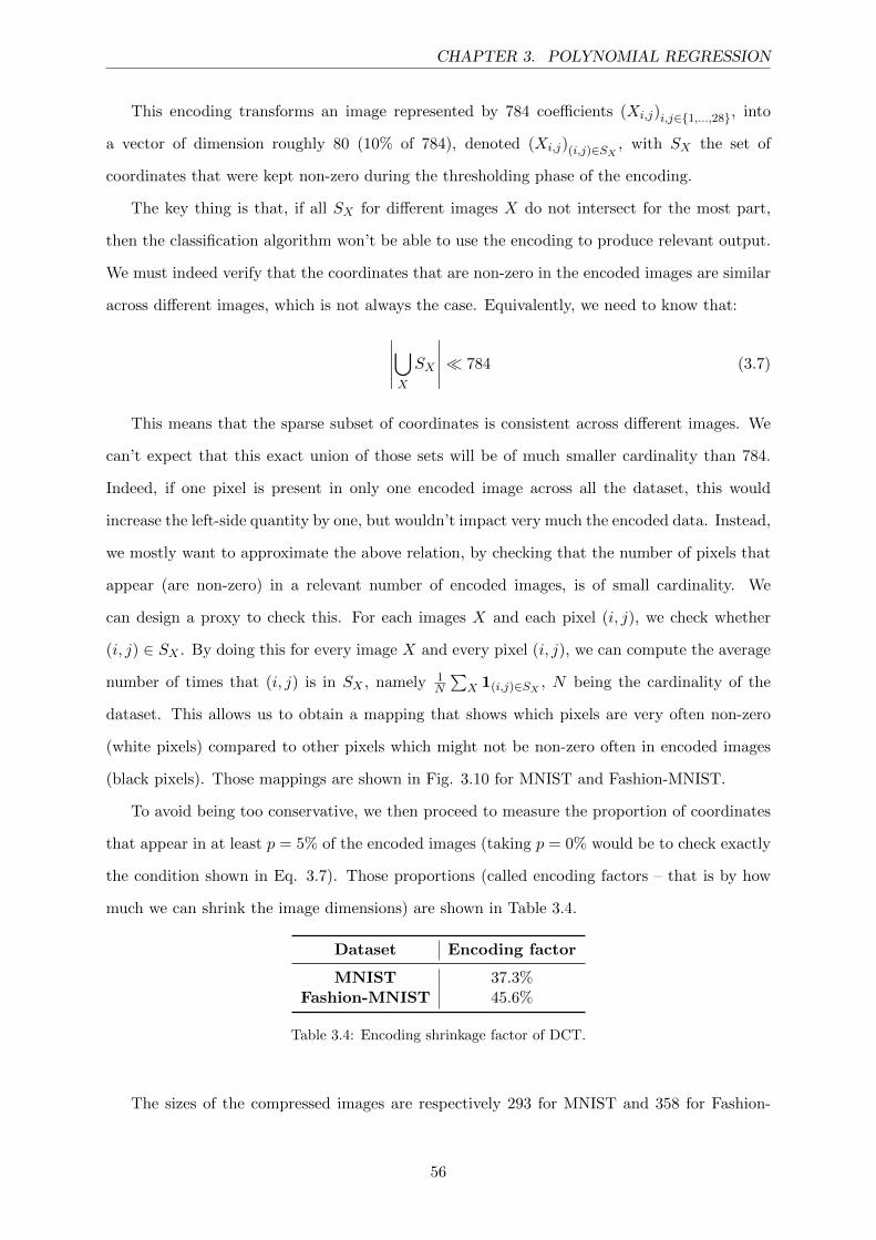
CHAPTER 3. POLYNOMIAL REGRESSION
This encoding transforms an image represented by 784 coefficients (Xi,j)i,j∈1,...,28, into
a vector of dimension roughly 80 (10% of 784), denoted (Xi,j)(i,j)∈SX, with SX the set of
coordinates that were kept non-zero during the thresholding phase of the encoding.
The key thing is that, if all SX for different images X do not intersect for the most part,
then the classification algorithm won’t be able to use the encoding to produce relevant output.
We must indeed verify that the coordinates that are non-zero in the encoded images are similar
across different images, which is not always the case. Equivalently, we need to know that:
∣∣∣∣∣⋃X
SX
∣∣∣∣∣ 784 (3.7)
This means that the sparse subset of coordinates is consistent across different images. We
can’t expect that this exact union of those sets will be of much smaller cardinality than 784.
Indeed, if one pixel is present in only one encoded image across all the dataset, this would
increase the left-side quantity by one, but wouldn’t impact very much the encoded data. Instead,
we mostly want to approximate the above relation, by checking that the number of pixels that
appear (are non-zero) in a relevant number of encoded images, is of small cardinality. We
can design a proxy to check this. For each images X and each pixel (i, j), we check whether
(i, j) ∈ SX . By doing this for every image X and every pixel (i, j), we can compute the average
number of times that (i, j) is in SX , namely 1N
∑X 1(i,j)∈SX
, N being the cardinality of the
dataset. This allows us to obtain a mapping that shows which pixels are very often non-zero
(white pixels) compared to other pixels which might not be non-zero often in encoded images
(black pixels). Those mappings are shown in Fig. 3.10 for MNIST and Fashion-MNIST.
To avoid being too conservative, we then proceed to measure the proportion of coordinates
that appear in at least p = 5% of the encoded images (taking p = 0% would be to check exactly
the condition shown in Eq. 3.7). Those proportions (called encoding factors – that is by how
much we can shrink the image dimensions) are shown in Table 3.4.
Dataset Encoding factor
MNIST 37.3%Fashion-MNIST 45.6%
Table 3.4: Encoding shrinkage factor of DCT.
The sizes of the compressed images are respectively 293 for MNIST and 358 for Fashion-
56
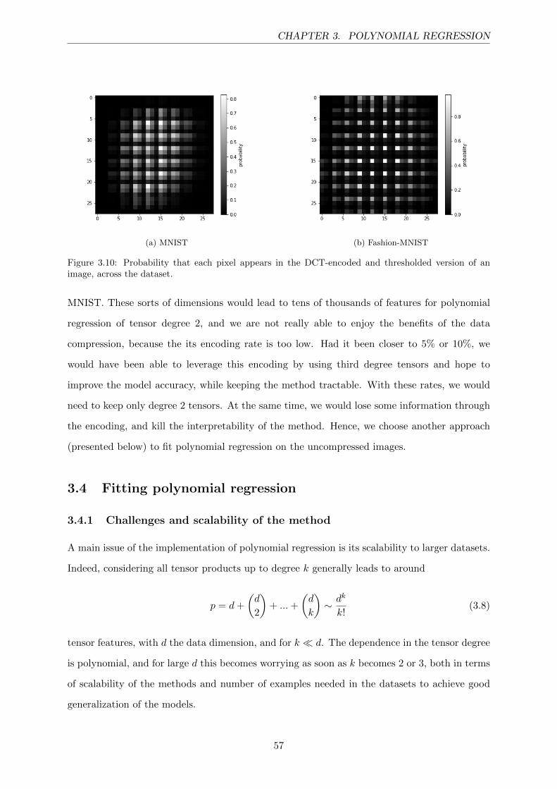
CHAPTER 3. POLYNOMIAL REGRESSION
(a) MNIST (b) Fashion-MNIST
Figure 3.10: Probability that each pixel appears in the DCT-encoded and thresholded version of animage, across the dataset.
MNIST. These sorts of dimensions would lead to tens of thousands of features for polynomial
regression of tensor degree 2, and we are not really able to enjoy the benefits of the data
compression, because the its encoding rate is too low. Had it been closer to 5% or 10%, we
would have been able to leverage this encoding by using third degree tensors and hope to
improve the model accuracy, while keeping the method tractable. With these rates, we would
need to keep only degree 2 tensors. At the same time, we would lose some information through
the encoding, and kill the interpretability of the method. Hence, we choose another approach
(presented below) to fit polynomial regression on the uncompressed images.
3.4 Fitting polynomial regression
3.4.1 Challenges and scalability of the method
A main issue of the implementation of polynomial regression is its scalability to larger datasets.
Indeed, considering all tensor products up to degree k generally leads to around
p = d+
(d
2
)+ ...+
(d
k
)∼ dk
k!(3.8)
tensor features, with d the data dimension, and for k d. The dependence in the tensor degree
is polynomial, and for large d this becomes worrying as soon as k becomes 2 or 3, both in terms
of scalability of the methods and number of examples needed in the datasets to achieve good
generalization of the models.
57

CHAPTER 3. POLYNOMIAL REGRESSION
Moreover, recall that standard linear regression computes the optimal coefficients as:
β =(XTX
)−1XTY (3.9)
where X ∈ Rn×p is the data and Y ∈ Rn×K are the (maybe multi-dimensional) labels, with
K the number of classes. Multiplying two matrices A ∈ Ra×b and B ∈ Rb×c requires O(abc)
operations. Inverting a matrix of size n with standard solvers generally requires O(n2.4) for the
best solvers. Hence, for n examples of dimension p, linear regression is solved with a complexity
of:
O(np2 + p2.4 + minnp2 + npK, npK + p2K
)(3.10)
Typically, K n, p, hence the complexity becomes approximately:
O(np2 + p2.4
)(3.11)
Overall, solving polynomial regression hence has a time complexity of:
O
(n
[dk
k!
]2+
[dk
k!
]2.4)(3.12)
where d is the original data dimension (784 in our case), and k the tensor degree. Memory is
also an issue, because the X matrix is very large (because of the high number of tensor features).
This makes polynomial regression difficult to fit perfectly in practice, and is why we resort in
the following parts to designing scalable heuristics that allow us to find a good quality solution
that generalizes well on the out-of-sample data.
3.4.2 Setup
Clearly, given the number of features in those datasets, we can’t, for now, scale to degree 3 tensor
products. We are then restricted to using at most degree 2 only tensor products. Moreover,
considering all degree 2 tensor products still creates way too many features (307,720) compared
to the size of the dataset, and also makes it challenging to fit the model.
Hence, we resort to a “convolutional” version of the regression, in a similar fashion to what
is done with CNNs in deep learning. More specifically, among all degree 2 products of the
form XiXj where i, j ∈ 1, ..., 282, we only consider those for which the two pixels i and j can
be covered simultaneously by a square filter of size 3 × 3. Otherwise said, we restrict the L1
58

CHAPTER 3. POLYNOMIAL REGRESSION
distance between i and j to be smaller or equal to 4 (which happens if the two pixels are covered
by opposite angles of the filter). This step drops the number of features to 18,740 (including
degree 1 “products”).
Our target function hence becomes:
minβ
∥∥∥∥∥∥∥∥Y − β0 −∑i
βiXi −∑i,j
L1(i,j)≤4
βi,jXiXj
∥∥∥∥∥∥∥∥2
2
(3.13)
where we slightly tweak notation once again, and where i, j are 2-dimensional vectors with
each coordinate in 1, ..., 28 (i and j are pixel coordinates). In the following, we include the
intercept as part of the Xβ term by introducing a constant column in X.
Our prediction model is constructed by stacking 10 different polynomial regression models,
one per class, according to Eq. 3.13. In particular, the choice of coefficients of for each class is
made independently. The regression model then outputs, for any test data, a Y ∈ R10 where Yi
is the predicted value for the class corresponding to index i. Finally, we predict the final class
based on the rule arg max16i610 Yi, namely the class that has the highest polynomial regression
output.
3.4.3 Introduction of batched linear regression as a scalable fitting method
In the regression problem minβ ‖Y −Xβ‖22, we are generally unable for polynomial regression
to compute in a scalable way the optimal solution β∗ =(XTX
)−1XTY over the whole dataset.
As seen in the following section, we are luckily still able to find this exact solution in the case
of MNIST and Fashion-MNIST, but this would not be doable for larger and more complex
datasets, hence we need to introduce another method.
We now introduce batched linear regression as a way to scale this process. Call B a batch
size, and NB a number of batches. We denote by XiB a random subset of rows of X of size
B, where i denotes the numbering of the draws (we will draw randomly multiple times). We
similarly define Y iB. In the following, each i = 1, ..., NB corresponds to a different random
sample of those rows. Now define βi to be the least-squares solution over the dataset restricted
to these rows, namely:
βi = arg minβ
∥∥Y iB −Xi
Bβ∥∥22
(3.14)
This βi is hence obtained from a subset of examples present in the dataset. As long as βi has an
59

CHAPTER 3. POLYNOMIAL REGRESSION
out-of-sample performance higher than that of a random model, then every individual model
should be useful, and hopefully encode different (or at least not linearly dependent) information
about the data. We run this process NB times, and then build the final polynomial regression
model denoted by β as an average of those models:
β =1
NB
NB∑i=1
βi (3.15)
Otherwise said, our strategy is to make each of the (sub-)linear regressions run on the sub-
sampled dataset tractable both in time and in memory, hoping that each “imperfect” (and
noisy) βi will contain relevant out-of-sample information. In the end, by averaging all those
noisy linear regressions, we are hoping to make use of the power of averaging to cancel out the
noise and obtain a satisfactory final model β without much noise in it. Of course, if B is chosen
to be too small, each βi will be pure noise and the final β will be close to 0. However, we observe
that, contrary to expectations, relatively small values of B (much smaller than the number of
tensor features) and NB can lead to very good performances. Note that this method is very
similar to methods using bootstrap aggregation (bagging), which typically train sub-models
on part of a dataset, and reconciliate the sub-models at the end of the training process (by
averaging them, or with another heuristic, such as voting in the case of random forests).
The results of the aforementioned heuristic batch training process for MNIST and Fashion-
MNIST datasets are reported in Figure 3.11. We have chosen NB = 60 and B = 2,000. Since
the datasets are of size 60,000, this will make us cover between once and twice the whole
dataset on average through all the (sub-)linear regressions. The rationale behind this choice is
to ensure that the maximal number B × NB of samples we have used throughout the process
is comparable with the size of the whole dataset (in practice, the effective number of samples
seen will be lower than B × NB). The accuracy we plot is evaluated on a random sample of
size 2,000 of the out-of-sample set (representing 20% of the out-of-sample dataset), for speed
purposes. The blue curve corresponds to the out-of-sample accuracy of each individual model
βi, for different i (fitted on different batches b of data). Now, for the orange curve, let us define:
βavgb =1
b
b∑i=1
βi (3.16)
such that β = βavgNB. The orange curve corresponds to the out-of-sample accuracy of βavgb , as a
60
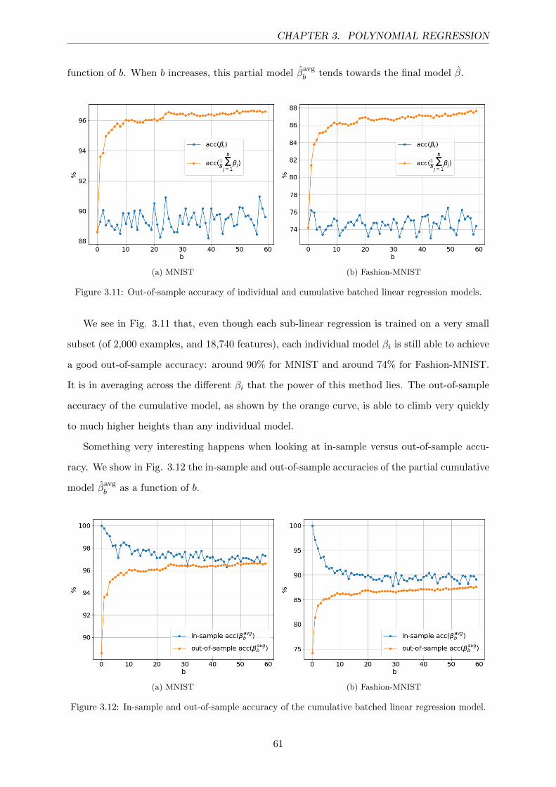
CHAPTER 3. POLYNOMIAL REGRESSION
function of b. When b increases, this partial model βavgb tends towards the final model β.
(a) MNIST (b) Fashion-MNIST
Figure 3.11: Out-of-sample accuracy of individual and cumulative batched linear regression models.
We see in Fig. 3.11 that, even though each sub-linear regression is trained on a very small
subset (of 2,000 examples, and 18,740 features), each individual model βi is still able to achieve
a good out-of-sample accuracy: around 90% for MNIST and around 74% for Fashion-MNIST.
It is in averaging across the different βi that the power of this method lies. The out-of-sample
accuracy of the cumulative model, as shown by the orange curve, is able to climb very quickly
to much higher heights than any individual model.
Something very interesting happens when looking at in-sample versus out-of-sample accu-
racy. We show in Fig. 3.12 the in-sample and out-of-sample accuracies of the partial cumulative
model βavgb as a function of b.
(a) MNIST (b) Fashion-MNIST
Figure 3.12: In-sample and out-of-sample accuracy of the cumulative batched linear regression model.
61
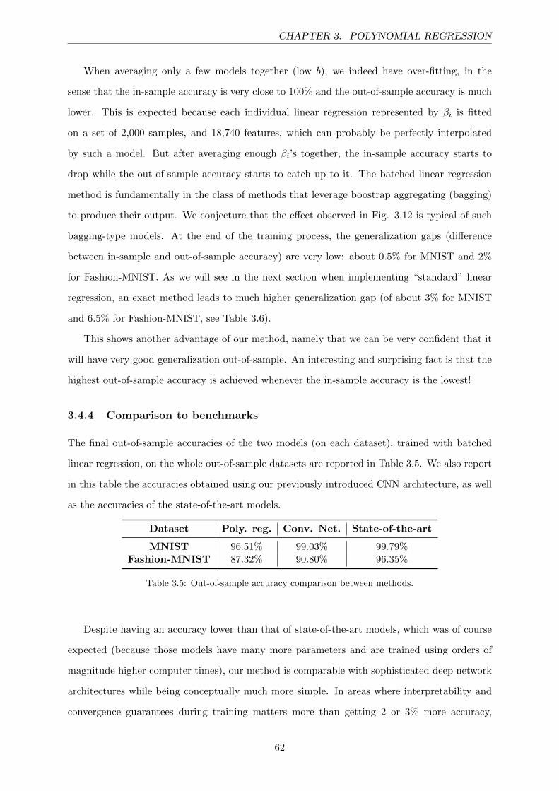
CHAPTER 3. POLYNOMIAL REGRESSION
When averaging only a few models together (low b), we indeed have over-fitting, in the
sense that the in-sample accuracy is very close to 100% and the out-of-sample accuracy is much
lower. This is expected because each individual linear regression represented by βi is fitted
on a set of 2,000 samples, and 18,740 features, which can probably be perfectly interpolated
by such a model. But after averaging enough βi’s together, the in-sample accuracy starts to
drop while the out-of-sample accuracy starts to catch up to it. The batched linear regression
method is fundamentally in the class of methods that leverage boostrap aggregating (bagging)
to produce their output. We conjecture that the effect observed in Fig. 3.12 is typical of such
bagging-type models. At the end of the training process, the generalization gaps (difference
between in-sample and out-of-sample accuracy) are very low: about 0.5% for MNIST and 2%
for Fashion-MNIST. As we will see in the next section when implementing “standard” linear
regression, an exact method leads to much higher generalization gap (of about 3% for MNIST
and 6.5% for Fashion-MNIST, see Table 3.6).
This shows another advantage of our method, namely that we can be very confident that it
will have very good generalization out-of-sample. An interesting and surprising fact is that the
highest out-of-sample accuracy is achieved whenever the in-sample accuracy is the lowest!
3.4.4 Comparison to benchmarks
The final out-of-sample accuracies of the two models (on each dataset), trained with batched
linear regression, on the whole out-of-sample datasets are reported in Table 3.5. We also report
in this table the accuracies obtained using our previously introduced CNN architecture, as well
as the accuracies of the state-of-the-art models.
Dataset Poly. reg. Conv. Net. State-of-the-art
MNIST 96.51% 99.03% 99.79%Fashion-MNIST 87.32% 90.80% 96.35%
Table 3.5: Out-of-sample accuracy comparison between methods.
Despite having an accuracy lower than that of state-of-the-art models, which was of course
expected (because those models have many more parameters and are trained using orders of
magnitude higher computer times), our method is comparable with sophisticated deep network
architectures while being conceptually much more simple. In areas where interpretability and
convergence guarantees during training matters more than getting 2 or 3% more accuracy,
62

CHAPTER 3. POLYNOMIAL REGRESSION
polynomial regression is to be considered as a viable alternative to deep learning methods.
3.4.5 Comparison to exact methods when tractable
In the case of datasets such as MNIST and Fashion-MNIST, for which the number of samples is
60,000 and the dimension of samples is 784, we were able, using powerful clusters, to fully scale
the method to be able to fit the linear regression objective without using the batched version
presented in the last section (which is able to run on much smaller infrastructures).
This procedure being both memory and time intensive for the specifications of these datasets,
we resorted to using clusters of machines with high-memory allowance, in order to be able to
compute the optimal linear regression weights. The fitting procedure takes of order hours and
uses tens of gigabytes of memory, which is not supported on standard personal computers.
In any case, this “exact” procedure should probably not be sought after too much, because
it becomes non-scalable on more complex datasets, for which the number of features would
be more typically of order thousands, and for which the tensor degree and filter size required
would be higher (creating in the end hundreds of thousands, if not millions, of polynomial
regression features). Moreover, for those more complex datasets, a huge number of samples
would be required to be able to obtain a satisfactory fit with some confidence on the out-
of-sample performance (typically a number of samples of order at least the number of tensor
features).
The “exact” linear regression surprisingly produces very similar results compared to the
batched linear regression presented above. The in-sample and out-of-sample accuracies on both
datasets are shown in Table 3.6.
Dataset In-sample Out-of-sample
MNIST 98.66% 95.81%Fashion-MNIST 94.39% 87.88%
Table 3.6: Performance of polynomial regression with “exact” linear regression fit.
Out-of-sample, the linear regression fit displays very similar accuracy to the batched lin-
ear regression fit. Standard linear regression performs slightly better on Fashion-MNIST and
slightly worse on MNIST, but overall the accuracies are very similar. However, raw coefficients
of the two methods are very different, especially in terms of scale. Let us define the L1 and L2
(which is the usual standard deviation) scaling functions as follow, where N is the dimension
63

CHAPTER 3. POLYNOMIAL REGRESSION
of x:
L1(x) =1
N
∑i
|xi −median(x)| (3.17)
L2(x) =
√1
N
∑i
(xi −mean(x))2 (3.18)
Applying those two measures on the vectors of linear regression coefficients (grouped together
across all classes) reveals the order of magnitude of those coefficients (giving more or less weight,
with L2 or L1 respectively, to extreme coefficients). The results are displayed in Table 3.7.
Dataset Batched regression L1 L2
MNIST No 1.9× 10⁹ 1.6× 10¹⁰
MNIST Yes 5.7× 10⁻³ 9.6× 10⁻³
Fashion-MNIST No 1.4× 10⁷ 6.9× 10⁷
Fashion-MNIST Yes 8.4× 10⁻³ 1.3× 10⁻²
Table 3.7: Magnitude of model coefficients for linear regression and batched linear regression.
The difference in the magnitude of the coefficients for the two methods (batched or standard
linear regression) is enormous, of order 1012 for MNIST and 109 for Fashion-MNIST. What
happens is that, on the edges of the images, pixels are black most of the time, with a value of 0.
Hence, having very large coefficients on the edges won’t impact the accuracy on most images.
Those coefficients are basically determined using the very few samples that don’t have only
black pixels in those extreme locations. On every single iteration of batched linear regression,
the same thing happens. However, because the coefficients are averaged over many batches,
this has the effect of shrinking down the magnitude of the coefficients on the edges.
This difference in the coefficients’ magnitude is worth mentioning, because it shows that
the standard linear regression method will be much less robust to the introduction of global
noise (see 3.6.2). Indeed, a very small perturbation in the digits of the image will produce an
very large change in the output of the model, leading to very poor performances under even
very small amounts of noise. That is one of the reasons why we decided to move forward with
the model fitted using our batched linear regression process. The batched linear regression
algorithm is much more scalable, and can be applied on problems involving much larger and
more complex datasets.
64

CHAPTER 3. POLYNOMIAL REGRESSION
3.5 Understanding gradient descent behavior
In fully-tractable cases (i.e. when the dimension of the data d is low), polynomial regression
allows us to obtain a good approximation of the functions computed by neural networks with
ReLU activation. In the case where the neural network has a polynomial activation, we even
showed that the approximation could be equality, by construction of the polynomial regression
method.
For a neural network defined by W , as defined in Eq. 3.1, we once again define the “equiv-
alent” tensor weights as the ones defined in Eq. 3.4. This allows us to transform the neural
network weights W into tensor weights W , as long as we have an polynomial approximation
(a0, ..., ak) of the activation function of the neural network. In the following, we will adopt the
same notations as above, and tensor weights of degree l will be denoted W(d)a1,...,al .
Being able to fit a linear model through polynomial regression grants more convergence
guarantees during training than fitting a non-convex function with heuristic procedures such as
SGD, which a widely used standard in the deep learning community. The problem of finding
what neural network weights converge to during this training process has proven to be a daunting
task, as mentioned in the section on previous work. Indeed, analyzing the dynamics of such
non-convex, non-linear, and random processes is not an easy task. However, in tractable cases,
we know that polynomial regression will converge to the global optimum, provided that the
number of samples is high enough (which is a very typical constraint for linear regression).
In this section, we adopt a reverse point of view in which we generate a random dataset using
a non-linear ReLU-activated neural network, and fit this dataset using polynomial regression.
We also train another neural network with ReLU activation on this dataset (this network should
be able – in theory – to perfectly recover the teacher network). Then, we compare the weights
obtained by the polynomial regression model to the equivalent tensor weights of the weights
in the trained student neural network. We are hoping to show that, for synthetic datasets,
the neural network weights correspond to nothing else but the optimal tensor weights obtained
through polynomial regression.
The synthetic datasets that we generate are created with a neural network with independent
normally distributed weights with standard deviation 1/√d (where d is the data dimension),
and bi = 1 for all i, to produce an output as defined in Eq. 3.1. The data X is generated
according to a standard normal distribution, with independent components. It is then passed
65

CHAPTER 3. POLYNOMIAL REGRESSION
through the random network to produce targets Y . This process is run twice to produce an
in-sample dataset and an out-of-sample dataset.
The final polynomial regression model is obtained by solving to optimum the standard least
squares objective, and we make sure that the sample size is high enough to obtain a unique
solution. The training process of the neural network is run using SGD (similarly to Algorithm
1, with T = 1), with a batch size of 100.
The dimension of the data generated is chosen as d = 20, and the neural networks have
a hidden layer of size m = 100. Choosing different architectures for the dataset-generating
network and for the student network doesn’t change the conclusion of this section.
Matching weights with a polynomial ReLU approximation prior
In order to be able to define equivalent tensor weights of the weights of the trained neural
network, we need to know a polynomial approximation of the ReLU function, which is the
activation function of the trained neural network. In order to obtain this approximation, recall
that because of the normalization of the weights, the following fact holds:
[W>X]i = O(1) (3.19)
Because the activation function is applied to this exact quantity, we can restrict our search of an
approximation of the ReLU function to the compact set [−3, 3] (because W and X are standard
normal, most values of [W>X]i will fall in this range).
We choose to use degree 3 tensors, because it is tractable in this low-dimensional data
setting. We then run a brute force (i.e. grid search) procedure over all polynomials of the form:
a0 + a1x+ a2x2 + a3x
3 (3.20)
with bounded coefficients |ai| ≤ 3. These coefficients are discretized on the [−3, 3]4 grid with
150 steps per dimension.
We then take the approximation (i.e. the set of polynomial coefficients) that leads to the
best (smallest) weighted L2 or L∞ distance between the ReLU function and the polynomial
approximation. The weights in the distance function are defined as the values of the PDF of
the normal distribution over the chosen interval of approximation, [−3, 3]. This means that we
give more weight to our approximation in the center of the interval, because most of the outputs
66

CHAPTER 3. POLYNOMIAL REGRESSION
[W>X]i will be in this area ([W>X]i follows the standard normal distribution N (0, 1), because
of the scaling of W and the independence of W and X). We repeat this loop twice, using a
tighter grid centered around the set of optimal polynomial coefficients found in the previous
step, when running a new loop. The two approximations we obtain are shown in Fig. 3.13.
Figure 3.13: Polynomial approximation of ReLU activation.
Because of the weighting, the approximations are indeed more precise around the center of
the interval. We also observe that the two approximations both have a positive bias around the
edges of the interval. The coefficients of the two polynomial approximations PL2 and PL∞ are:
PL2(x) = 0.188 + 0.5x+ 0.21x2 + 1.39× 10⁻¹⁷ · x3 (3.21)
for the L2 distance approximation, and:
PL∞(x) = 0.096 + 0.5x+ 0.3x2 − 2.77× 10⁻¹⁷ · x3 (3.22)
for the L∞ distance approximation. We see that the degree 3 coefficient is very small. This
makes sense considering the dependence of the median recovery R2 on the tensor degree, as we
showed in Table 3.1. Going from tensor degree 2 to tensor degree 3 in polynomial regression
did not bring much value when working with ReLU activation. That means the weights corre-
sponding to degree 3 tensors in the polynomial regression must have been very small. Since, as
shown in the definition of tensor weights W (3), a3 appears in front of all of them, that means
a3 must be small, which is what we find to be the case, using this brute force approach.
Here, with dimension d = 20 and degree 3 tensors, the number of features is 1,770. We
generate N = 50,000 examples in the training set, to make sure that our polynomial regression
model uses a number of samples higher than the sample complexity (which is usually equal to
67
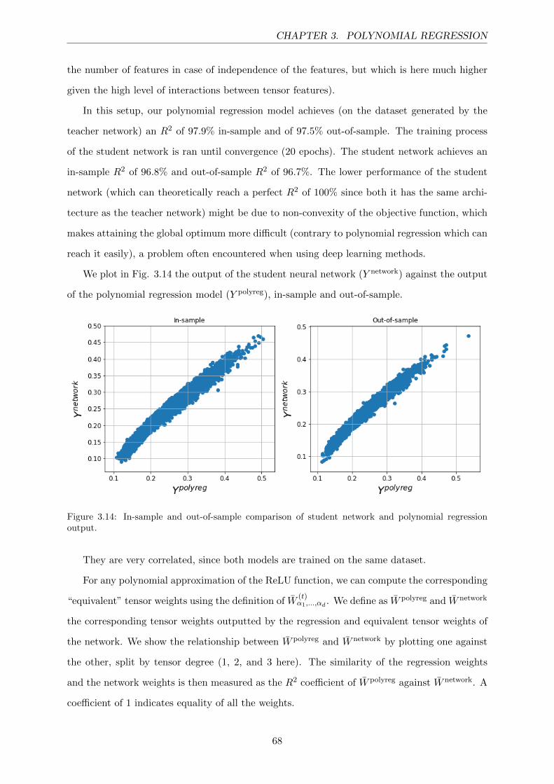
CHAPTER 3. POLYNOMIAL REGRESSION
the number of features in case of independence of the features, but which is here much higher
given the high level of interactions between tensor features).
In this setup, our polynomial regression model achieves (on the dataset generated by the
teacher network) an R2 of 97.9% in-sample and of 97.5% out-of-sample. The training process
of the student network is ran until convergence (20 epochs). The student network achieves an
in-sample R2 of 96.8% and out-of-sample R2 of 96.7%. The lower performance of the student
network (which can theoretically reach a perfect R2 of 100% since both it has the same archi-
tecture as the teacher network) might be due to non-convexity of the objective function, which
makes attaining the global optimum more difficult (contrary to polynomial regression which can
reach it easily), a problem often encountered when using deep learning methods.
We plot in Fig. 3.14 the output of the student neural network (Y network) against the output
of the polynomial regression model (Y polyreg), in-sample and out-of-sample.
Figure 3.14: In-sample and out-of-sample comparison of student network and polynomial regressionoutput.
They are very correlated, since both models are trained on the same dataset.
For any polynomial approximation of the ReLU function, we can compute the corresponding
“equivalent” tensor weights using the definition of W(t)α1,...,αd . We define as W polyreg and W network
the corresponding tensor weights outputted by the regression and equivalent tensor weights of
the network. We show the relationship between W polyreg and W network by plotting one against
the other, split by tensor degree (1, 2, and 3 here). The similarity of the regression weights
and the network weights is then measured as the R2 coefficient of W polyreg against W network. A
coefficient of 1 indicates equality of all the weights.
68

CHAPTER 3. POLYNOMIAL REGRESSION
The weights obtained with the network using the L2 approximation of the ReLU function
are used in Fig. 3.15, while the weights obtained with the network using the L∞ approximation
of the ReLU function are used in Fig. 3.16. The red line corresponds to a perfect matching
between the weights.
Figure 3.15: Neural network “equivalent” tensor weights vs. polynomial regression weights with ReLUL2 polynomial approximation.
Figure 3.16: Neural network “equivalent” tensor weights vs. polynomial regression weights with ReLUL∞ polynomial approximation.
The corresponding R2 (similarity between the network and regression weights) are shown in
Table 3.8.
Approximation type Degree 1 Degree 2 Degree 3
L2 99.83% 81.5% 0.26%L∞ 99.84% 96.5% 0.26%
Table 3.8: Similarity (R2) between polynomial regression weights and neural network “equivalent” tensorweights with various polynomial approximations of the ReLU activation.
As seen in this table, there is an almost perfect matching between the degree 1 weights.
With degree 2 weights, the matching is good but not as perfect. It is improved a lot by using
the L∞ polynomial approximation of the ReLU activation instead of the L2 one, which might
provide a hint that the L∞ norm might be a better representation, in our problem, of how the
69
CHAPTER 3. POLYNOMIAL REGRESSION
ReLU activation should be approximated by a polynomial. Notice though that the matching
is not perfect for the degree 2 weights, even using the L∞ approximation. For the degree 3
weights, recall that our grid search approximation of the ReLU yielded a very small degree 3
coefficient a3. Using the definition of W (3), that implies that W (3) is also very small. As seen
in both Fig. 3.15 and Fig. 3.16, the degree 3 equivalent tensor weights of the network are
indeed all very close to 0. The problem is that the grid search approach fundamentally misses
many points (because it is a grid), and hence many polynomial coefficients are not considered.
Because the optimal a3 coefficient is probably very close to 0, it is likely that the grid search
approach would have a hard time finding this optimum.
Matching weights using a posterior inferred polynomial ReLU approximation
Computing the right prior polynomial approximation of the ReLU function is a hard task.
Indeed, we don’t really know which kind of objective function we should be minimizing (such as
the L2 norm or the L∞ norm) between the ReLU function and the approximating polynomial.
Instead, recall the definition of tensor weights:
W (t)α1,...,αd
= at
m∑i=1
Wα11,i ...W
αdd,i (3.23)
Since all the quantities except at in this equation are known (W are the weights of the network,
and m the hidden dimension is also known), what we can do is infer a posteriori the value of
at that brings the polynomial regression weights and “equivalent” tensor weights of the neural
network the closest to each other. Namely, what we seek to optimize is:
mina
∑α1,...,αd∑
i αi=t
∥∥∥∥∥W reg,(t)α1,...,αd
− am∑i=1
Wα11,i ...W
αdd,i
∥∥∥∥∥2
2
(3.24)
where Wreg,(t)α1,...,αd are the polynomial regression weights. This is a one-dimensional regression and
the optimal coefficient a is the beta of the regression weights over the network weights (or more
precisely their tensor equivalents), where:
β(x, y) =
∑i xiyi∑i x
2i
(3.25)
70

CHAPTER 3. POLYNOMIAL REGRESSION
Running this program for each degree t = 1, 2, 3 (as well as using the intercept of the model as
the coefficient a0) yields a polynomial ReLU approximation of the form:
Pposterior(x) = 0.114 + 0.498x+ 0.352x2 − 1.1× 10⁻³ · x3 (3.26)
This polynomial is indeed more similar to the L∞ approximation. That confirms why the this
approximation performed better when using a prior of the ReLU function. A plot of those three
approximations is shown in Fig. 3.17.
Figure 3.17: Polynomial approximation of ReLU activation (priors and posterior).
One can see that the red and orange curves are indeed similar to each other. However, the
use of a posterior approximation of the ReLU activation allows us to improve the matching of
the weights, as shown in Fig. 3.18.
Figure 3.18: Neural network “equivalent” tensor weights vs. polynomial regression weights with ReLUposterior polynomial approximation.
This time, the weights at degree 2 match almost perfectly. Table 3.9 recapitulates the
similarities of the weights at each degree for the posterior approximation.
These results confirm that the degree 3 tensor weights must not matter very much in the
case of a neural network with ReLU activation. Running the same process for dimension d = 5,
71

CHAPTER 3. POLYNOMIAL REGRESSION
Approximation type Degree 1 Degree 2 Degree 3
Posterior 99.84% 98.53% 0.31%
Table 3.9: Similarity (R2) between polynomial regression weights and neural network “equivalent” tensorweights with using a posterior approximation of the ReLU activation.
for which a tensor degree of 4 is easily tractable, confirms this fact. In this case, the similarity
of tensor weights of degree 4 reaches almost 78%, while the one at degree 3 stays very low.
This supports the conjecture that the degree 3 coefficient in a polynomial approximation of the
ReLU activation should be very close to 0.
This section demonstrates that the SGD algorithm makes the weights of the neural network
converge towards the optimal polynomial regression tensor weights. Recall that, by construction,
polynomial regression is more powerful than any neural network with any smooth activation
function as soon as the tensor degree used is high enough (because then we can get better
and better polynomial approximations of the activation function). Hence, by converging to the
optimal polynomial regression weights, the SGD algorithm gets closer to a more powerful class
of function, and hence brings the performance of the neural network higher. This might be one
of the reasons for the good performance in practice of an algorithm such as SGD.
3.6 Advantages
3.6.1 Interpretability
A first and paramount advantage of our polynomial regression method is the fact that it is
fully and easily interpretable, by cleverly designing some heuristics to visualize the polynomial
regression coefficients.
In the following, we will index all the polynomial regression coefficients by quantities in R2.
For example, βi will denote the coefficient of the pixel i = (a, b), that is, the pixel located at
coordinates (a, b) in the image. We will refer to βi as a degree 1 coefficient, because it involves
only one pixel. Similarly, we denote Xi the ith pixel of image X. Hence, in a degree 2 polynomial
regression model as presented above, the output Y of the regression model writes (ignoring the
intercept):
Y =∑i
βiXi +∑i,j
βi,jXiXj (3.27)
For degree 2 terms, in the models using batched linear regression as mentioned in the previous
72

CHAPTER 3. POLYNOMIAL REGRESSION
section, we used only products of pixels that could be covered by a square filter of size 3 by
3, hence most βi,j were 0 (for i and j such that the L1 distance between the two is greater or
equal to 5, βi,j = 0).
Degree 1 coefficients
It is straight-forward to interpret the degree 1 coefficients, because there are exactly 784 coef-
ficients of the form βi, which is the same size as the images in the dataset. We can then plot,
for each class, the β coefficients in a 28 × 28 grid, where the position in the grid matches the
index of the coefficient. We show, for the models obtained via batched linear regression, on
both datasets, the results in Fig. 3.19.
(a) MNIST (b) Fashion-MNIST
Figure 3.19: Interpretation of degree 1 coefficients for polynomial regression.
Red coefficients are positives ones, while blue ones are negative. A red coefficient in some
73

CHAPTER 3. POLYNOMIAL REGRESSION
position means that, if a white pixel was at this position, this pixel would increase the likelihood
of the image being classified in this class by the polynomial regression model.
Obviously, since classes intersect each other (only having white pixels in a given area doesn’t
imply that an image belongs to a certain class), red pixels don’t cover all the shape of the object
represented by a class. The positive coefficients rather point out the specificity of each class, by
indicating which pixels should be found in a class, and should only be found in such class. This
can be seen in the Fashion-MNIST sneaker example, where pixels on the heel are much more
important than anywhere else on the sneaker. Similarly, for the digit 8 of MNIST for example,
only the two holes in the 8 shape are highlighted and denoted as important features of such a
digit. Several other similar interpretations can be done on other classes.
Degree 2 coefficients
Let us now turn to the interpretation of degree 2 coefficients βi,j . Without considering the
filtering that we applied to these coefficients, that made most of them 0, there would be 7842 =
614,656 of them (all pairs of pixels). Showing those coefficients directly in a 784 × 784 grid
would break the geometry, since coefficients corresponding to two pairs of pixels close to each
other could be shown very far apart on such grid. Moreover, in practice we only have 17,956
(= 18,740−784) of those coefficients that are non-zero. On such a grid, only a very thin diagonal
part would be shown as non-zero.
To remedy those issues, we design a heuristic that allows us to transform the degree 2
coefficients βi,j to be able to plot them in another 28×28 grid, like we did for degree 1 coefficients.
More explicitly, take a coefficient βi,j corresponding to pixels Xi and Xj . Denote i = (a, b) and
j = (c, d) the coordinates of those pixels, with a, b, c, d ∈ 1, ..., 28, in the original image. Now
define the coordinates k =(ba+c2 c, b
b+d2 c)
= f(i, j), where f is the function that “averages” two
pixels coordinates. Now, for each m,n ∈ 1, ..., 28, define, with k = (m,n):
B(m,n) =∑
i,j s.t.f(i,j)=k
βi,j (3.28)
which means that B is now a 28 × 28 matrix. Each of its entries contain the sum of all the
betas that correspond to a pair of pixels whose center of gravity is the entry itself. Because
only close-by pairs of pixels are considered, we are assured that B(k) cannot contain any term
βi,j with i or j very far from k. It is also guaranteed that we are not breaking the geometry
74

CHAPTER 3. POLYNOMIAL REGRESSION
of the coefficients. This local grouping allows to transform the 784× 784 matrix of coefficients
into a 28× 28 one. We show in Fig. 3.20 such grid B for each class, and both datasets.
(a) MNIST (b) Fashion-MNIST
Figure 3.20: Interpretation of degree 2 coefficients for polynomial regression.
Those figures become much more noisy, because of the heuristic and the task itself (fitting
degree 2 coefficients is harder, and degree 2 tensors also bring less value to the model than degree
1 ones). The interpretation is the following: red pixels correspond to areas where, if nearby
pixels have the same color (all black or all white), then it impacts positively the probability
that the image is in the class. Blue pixels do the same, but for areas where nearby pixels have
very different values. Hence, borders of the objects should be represented by blue pixels, while
dense white areas should be represented by red areas. In Fashion MNIST, for the sneaker class,
we can see how the blue border draws the shape of the sneaker, and similarly in the pullover or
trouser class. Deciphering the results is more challenging for the MNIST dataset in this case.
75

CHAPTER 3. POLYNOMIAL REGRESSION
3.6.2 Robustness to noise
Another advantage of polynomial regression over commonly used deep learning models is its
robustness to noise. The intuition is that simpler models might be less sensitive to the intro-
duction of noise in the out-of-sample data. One reason for this is that the gradients of the
model against any input coordinate would be lower in the case of polynomial regression (those
gradients are the coefficients of the linear regression model) compared to deep learning models,
which can display local gradient explosion. Here, models are still trained on noiseless data. We
do not expect results to change for the worse for polynomial regression if the training was done
on noisy data as well (deep learning models get very challenging to train in noisy environments).
To measure the robustness of models, we modify the images in two different ways. The two
image modifications that we apply are either to change every pixel by a “small” amount (global
noise), or change the pixels only in a smaller region, where each pixel is allowed to change
by a “large” amount (local noise). These modifications are in line with existing literature on
adversarial examples (see [SSRD19]).
Global noise
In the global noise setting, we perturb each image by adding, to each pixel, a random noise
drawn i.i.d. from the Gaussian distribution with mean zero and standard deviation σ. We then
truncate the result for each pixel to [0, 1], to ensure that the resulting image is still gray-scale.
An example of images after applying this global noise can be seen in Fig. 3.21, for σ = 0.3.
(a) MNIST (b) Fashion-MNIST
Figure 3.21: Images after applying the global noise modification, for σ = 0.3.
76

CHAPTER 3. POLYNOMIAL REGRESSION
Local noise
In the local noise setting, we add a rectangular black patch to the image. More specifically, for
a given patch area A, we first choose a random pixel location (i, j) uniformly around the center
of the image (6 6 i, j 6 22), and an aspect ratio D, uniformly distributed on (12 , 2). We then
create a patch centered at (i, j), of width w = bD√Ac and height h = b
√A/Dc. For each pixel
covered by the patch, we set its value to 0 (i.e. make it black). An example of images after
applying this local noise can be seen in Fig. 3.22, for A = 100.
(a) MNIST (b) Fashion-MNIST
Figure 3.22: Images after applying the local noise modification, for A = 100.
Note that, because there is some rounding while choosing the patch, its area can slightly
differ from A. The rationale for restricting the center position of patch to is to ensure that, on
average, a patch does not cover the dark background region of the images, but covers the region
with more informative content, e.g. the center of the image.
Measuring robustness
How to measure the robustness of a model is not obvious. One thing that is clear is that
models with a constant output should be considered as the most robust ones (because their
output doesn’t change in any condition). However, a constant model on the MNIST or Fashion-
MNIST would only achieve on average 10% accuracy. Looking at the accuracy of a model under
various noise levels is therefore not enough to evaluate its robustness. Instead, we also consider
the relative drop in accuracy as a function of the noise level. Namely, for a model with accuracy
77

CHAPTER 3. POLYNOMIAL REGRESSION
A(0) in a noiseless environment, and accuracy of A(n) in an environment with a noise-level of
n, we consider the quantity A(0)−A(n)A(0) . This quantity should be negative (adding noise shouldn’t
improve the accuracy of a model). It is also 0 for constant models (because A(0) = A(n) for any
n for those models). The interpretation is that a more robust model could have always lower
accuracy than another model, but with an unchanged accuracy when increasing the noise level
(for example a constant model against a deep learning model).
(a) MNIST - accuracy (b) MNIST - accuracy drop
(c) Fashion MNIST - accuracy (d) Fashion MNIST - accuracy drop
Figure 3.23: Accuracy and relative accuracy drop vs. noise standard deviation σ in the global noisesetting.
We plot in Fig. 3.23 and Fig. 3.24 both the accuracy as a function of the noise level, and,
what should be looked at more closely, the relative accuracy drop as a function of the noise,
as defined above. For the global noise, we plot those quantities against σ, while for the local
“patching” noise, we plot them against the area A of the path. In both cases, the higher the
curve, the better the model.
Our results show essentially the following facts:
• while the CNN architecture still achieves a higher prediction accuracy when the noise level
78

CHAPTER 3. POLYNOMIAL REGRESSION
(a) MNIST - accuracy (b) MNIST - accuracy drop
(c) Fashion MNIST - accuracy (d) Fashion MNIST - accuracy drop
Figure 3.24: Accuracy and relative accuracy drop vs. patch area A in the local noise setting.
is small (which is because of an obvious reason, namely that the deep learning model starts
with higher accuracy in the noiseless setting, hence it keeps its higher accuracy for small
noise levels), polynomial regression method starts outperforming the CNN architectures
once the noise level is increased beyond a certain level.
• when looking at robustness (i.e. relative accuracy drop instead of pure accuracy), the
polynomial regression model always achieves a higher robustness than the deep learning
CNN model.
• the results are consistent across both datasets and both noise-adding methods. The dif-
ference in robustness between the two models is even higher in the case of Fashion-MNIST
for the global noise setting.
• looking at accuracy or relative accuracy drop doesn’t matter much in the case of MNIST,
because the two models have very high and very similar accuracies in the noiseless set-
79

CHAPTER 3. POLYNOMIAL REGRESSION
ting. However, for the Fashion-MNIST dataset, the CNN model starts with an edge over
the polynomial regression model. In the case of patching (local noise), as seen in Fig.
3.24 graph (c), the CNN model is able to keep its edge in accuracy over the polyno-
mial regression model. However, the pace at which its accuracy decreases is faster than
for the polynomial regression model, which translates into a higher curve for polynomial
regression when looking at relative accuracy drop in graph (d).
• in terms of pure accuracy, the CNN model starts performing worse than the polynomial
regression model when, in the global noise setting, σ is increased beyond 0.3, and in the
local noise setting, when A is larger than 55 (which corresponds to roughly 7% of the
image being covered by a black patch, on average).
We believe that the aforementioned findings are a consequence of the simplicity of the
polynomial regression algorithm (which is a linear regression in high dimension), in contrast to
CNN architectures (which contain many non-linearities).
80

Chapter 4
Conclusion
In this report, we were able to derive a very simple order of magnitude formula for the sample
complexity of neural networks with one hidden layer. It is found to be linear in the input dimen-
sion and logarithmic in the width of the network. This is a first hint as to why neural networks
are still able to achieve good out-of-sample performance even in an over-parametrization setting
– namely because the number of examples needed to train the network in those setting grows
exponentially slower than the number of parameters.
Then, we introduced polynomial regression as a way to approximate neural networks through
the approximation of their activation function by a polynomial. The main challenge of this
method is its scalability, and we are able to design a heuristic that allows us to find approximate
tensor weights that are shown to have similar out-of-sample performance as the optimal ones,
and is competitive with deep learning architecture on MNIST datasets. Many advantages of
this method, advantages that usual deep learning methods lack, were studied. First, polynomial
regression has a very simple training objective, which is a linear function is the lifted space of
tensor products, and is equivalent to a linear regression in this space. Second, this method is
more robust than usual deep learning architectures to both local noise and global noise. Finally,
a polynomial regression model is shown to be very easy to interpret – separately for each tensor
degree – through direct representation of the weights or via heuristics.
Future work is still required on the main challenge of polynomial regression: its scalability.
In this report, we were able to scale training algorithms to very simple image datasets. However,
on more complex datasets such as ImageNet, those methods will probably have to be even more
optimized in order to scale to images containing tens of thousands of pixels (instead of less
than a thousand for the datasets considered here). A generalization would be to extend the
81

CHAPTER 4. CONCLUSION
polynomial regression approach to approximate multi-layer neural networks as well. It would be
fundamentally the same idea, except that the lifted space of tensor products would be a tensor
product of two spaces of simpler tensor products (in the case of a neural network with two
hidden layers). Apart from scalability, the whole analysis and its conclusions should generally
remain the same in this setup. Overall, tensor products seem to capture a lot of meaningful out-
of-sample information on quite challenging datasets, and, because of the numerous advantages
of polynomial regression, this method should be given more consideration in future directions
of research in the area of deep learning.
82

Bibliography
[ABA13] A. Auffinger and G. Ben Arous. Complexity of random smooth functions on the
high-dimensional sphere. arXiv:1110.5872, 2013.
[ABAC10] A. Auffinger, G. Ben Arous, and J. Cerny. Random matrices and complexity of
spin glasses. arXiv:1003.1129, 2010.
[ACGH18] S. Arora, N. Cohen, N. Golowich, and W. Hu. A convergence analysis of gradient
descent for deep linear neural networks. arXiv:1810.02281, 2018.
[ADH+19] Sanjeev Arora, Simon S Du, Wei Hu, Zhiyuan Li, Russ R Salakhutdinov, and
Ruosong Wang. On exact computation with an infinitely wide neural net. In
Advances in Neural Information Processing Systems, pages 8139–8148, 2019.
[AGMR16] S. Arora, R. Ge, T. Ma, and A. Risteski. Provable learning of noisy-or networks.
arXiv:1612.08795, 2016.
[AHW96] P. Auer, M. Herbster, and M. K. Warmuth. Exponentially many local minima for
single neurons. Advances in neural information processing systems, 1996.
[BCB15] D. Bahdanau, K. Cho, and Y. Bengio. Neural machine translation by jointly
learning to align and translate. Proceedings of the International Conference on
Learning Representations, 2015.
[Ben09] Y. Bengio. Learning deep architectures for ait. Foundations and Trends in Machine
Learning, 2(1):1–127, 2009.
[BG17] A. Brutzkus and A. Globerson. Globally optimal gradient descent for a convnet
with gaussian inputs. arXiv:1702.07966, 2017.
83

BIBLIOGRAPHY
[BHL18] Peter Bartlett, Dave Helmbold, and Phil Long. Gradient descent with identity ini-
tialization efficiently learns positive definite linear transformations. International
Conference on Machine Learning, pages 520–529, 2018.
[BSF94] Y. Bengio, P. Simard, and P. Frasconi. Learning long-term dependencies with
gradient descent is difficult. IEEE Transactions on Neural Networks, 5(2):157–
166, 1994.
[CHM+15] A. Choromanska, M. Henaff, M. Mathieu, G. B. Arous, and Y. LeCun. The loss
surfaces of multilayer networks. Artificial Intelligence and Statistics, 2015.
[CSS16] N. Cohen, O. Sharir, and A. Shashua. On the expressive power of deep learning:
A tensor analysis. Conference on Learning Theory, 2016.
[CT05] E. Candes and T. Tao. Decoding by linear programming. IEEE Transactions on
Information Theory, 51(12):4203–4215, 2005.
[Cyb89] G. Cybenko. Approximation by superpositions of a sigmoidal function. Mathe-
matics of control, signals and systems, 2(4):303–314, 1989.
[DLT17a] S. S. Du, J. D. Lee, and Y. Tian. Gradient descent learns one-hidden-layer cnn:
Don’t be afraid of spurious local minima. arXiv:1712.00779, 2017.
[DLT17b] S. S. Du, J. D. Lee, and Y. Tian. When is a convolutional filter easy to learn?
arXiv:1709.06129, 2017.
[DZPS18] S. S. Du, X. Zhai, B. Poczos, and A. Singh. Gradient descent provably optimizes
over-parameterized neural networks. arXiv:1810.02054, 2018.
[EGKZ20] M. Emschwiller, D. Gamarnik, E. Kizildag, and I. Zadik. Neural networks
and polynomial regression. demystifying the overparametrization phenomena.
arXiv:2003.10523, 2020.
[FCL18] H. Fu, Y. Chi, and Y. Liang. Local geometry of one-hidden-layer neural networks
for logistic regression. arXiv:1802.06463, 2018.
[GBB11] X. Glorot, A. Bordes, and Y. Bengio. Deep sparse rectifier neural networks. Pro-
ceedings of the 14th International Conference on Artificial Intelligence and Statis-
tics, 2011.
84
BIBLIOGRAPHY
[GHJY15] R. Ge, F. Huang, C. Jin, and Y. Yuan. Escaping from saddle points - online
stochastic gradient for tensor decomposition. Conference on Learning Theory,
2015.
[GK17] Surbhi Goel and Adam Klivans. Learning neural networks with two nonlinear
layers in polynomial time. arXiv preprint arXiv:1709.06010, 2017.
[GKKT16] S. Goel, V. Kanade, A. Klivans, and J. Thaler. Reliably learning the relu in
polynomial time. arXiv:1611.10258, 2016.
[GLM17] R. Ge, J. D. Lee, and T. Ma. Learning one-hidden-layer neural networks with
landscape design. arXiv:1711.00501, 2017.
[HDY+12] G. Hinton, L. Deng, D. Yu, G. E. Dahl, A.-r. Mohamed, N. Jaitly, A. Senior,
V. Vanhoucke, P. Nguyen, T. N. Sainath, and et al. Deep neural networks for
acoustic modeling in speech recognition: The shared views of four research groups.
IEEE Signal Processing Magazine, 29(6):82–97, 2012.
[HM16] M. Hardt and T. Ma. Identity matters in deep learning. arXiv:1611.04231, 2016.
[HN10] G. Hinton and V. Nair. Rectified linear units improve restricted boltzmann ma-
chines. Proceedings of the 27th International Conference on Machine Learning,
2010.
[Hoc98] S. Hochreiter. The vanishing gradient problem during learning recurrent neural
nets and problem solutions. International Journal of Uncertainty, Fuzziness and
Knowledge-Based Systems, 6(2):107–116, 1998.
[Hor91] K. Hornik. Approximation capabilities of multilayer feedforward networks. Neural
networks, 4:251–257, 1991.
[HZRS15] K. He, X. Zhang, S. Ren, and J. Sun. Delving deep into rectifiers: Surpassing
human-level performance on imagenet classification. ICCV, 2015.
[JGH18] Arthur Jacot, Franck Gabriel, and Clement Hongler. Neural tangent kernel: Con-
vergence and generalization in neural networks. In Advances in neural information
processing systems, pages 8571–8580, 2018.
85

BIBLIOGRAPHY
[JGN+17] C. Jin, R. Ge, P. Netrapalli, S. M. Kakade, and M. I. Jordan. How to escape
saddle points efficiently. arXiv:1703.00887, 2017.
[JSA15] M. Janzamin, H. Sedghi, and A. Anandkumar. Beating the perils of non-convexity:
Guaranteed training of neural networks using tensor methods. arXiv:1506.08473,
2015.
[Kaw16] K. Kawaguchi. Deep learning without poor local minima. Advances in Neural
Information Processing Systems, 2016.
[KKSK11] S. M. Kakade, V. Kanade, O. Shamir, and A. Kalai. Efficient learning of general-
ized linear and single index models with isotonic regression. Advances in Neural
Information Processing Systems, 2011.
[KS09] A. T. Kalai and R. Sastry. The isotron algorithm: High-dimensional isotonic
regression. COLT, 2009.
[KSH12] A. Krizhevsky, I. Sutskever, and G. Hinton. Imagenet classification with deep con-
volutional neural networks. Advances in Neural Information Processing Systems,
25:1097–1105, 2012.
[LBBH98] Yann LeCun, Leon Bottou, Yoshua Bengio, and Patrick Haffner. Gradient-based
learning applied to document recognition. In Proceedings of the IEEE, pages 2278–
2324, 1998.
[LeC98] Yann LeCun. The mnist database of handwritten digits.
http://yann.lecun.com/exdb/mnist/, 1998.
[LLS+18] M. Liu, S. Liu, H. Su, K. Cao, and J. Zhu. Analyzing the noise robustness of deep
neural networks. IEEE Conference on Visual Analytics Science and Technology,
pages 60–71, 2018.
[LPW+17] Z. Lu, H. Pu, F. Wang, Z. Hu, and L. Wang. The expressive power of neural
networks: A view from the width. arXiv:1709.02540, 2017.
[LRZ19] Tengyuan Liang, Alexander Rakhlin, and Xiyu Zhai. On the risk of minimum-
norm interpolants and restricted lower isometry of kernels. arXiv preprint
arXiv:1908.10292, 2019.
86
BIBLIOGRAPHY
[LY17] Y. Li and Y. Yuan. Convergence analysis of two-layer neural networks with relu
activation. arXiv:1705.09886, 2017.
[MHN13] Andrew L. Maas, Awni Y. Hannun, and Andrew Y. Ng. Rectifier nonlinearities
improve neural network acoustic models. ICML Workshop on Deep Learning for
Audio, Speech and Language Processing, 2013.
[MMN18] S. Mei, A. Montanari, and P.-M. Nguyen. A mean field view of the landscape
of two-layers neural networks. Proceedings of the National Academy of Sciences,
2018.
[NH17] Q. Nguyen and M. Hein. The loss surface of deep and wide neural networks.
arXiv:1704.08045, 2017.
[PLR+16] B. Poole, S. Lahiri, M. Raghu, Sohl-Dickstein J., and S. Ganguli. Exponential
expressivity in deep neural networks through transient chaos. Advances In Neural
Information Processing Systems, 2016.
[RPK+16] M. Raghu, B. Poole, J. Kleinberg, S. Ganguli, and J. Sohl-Dickstein. On the
expressive power of deep neural networks. arXiv:1606.05336, 2016.
[SA14] H. Sedghi and A. Anandkumar. Provable methods for training neural networks
with sparse connectivity. arXiv:1412.2693, 2014.
[SC16] D. Soudry and Y. Carmon. No bad local minima: Data independent training error
guarantees for multilayer neural networks. arXiv:1605.08361, 2016.
[Sha16] O. Shamir. Distribution-specific hardness of learning neural networks.
arXiv:1609.01037, 2016.
[Sha18] O. Shamir. Exponential convergence time of gradient descent for one-dimensional
deep linear neural networks. arXiv:1809.08587, 2018.
[SHM+16] D. Silver, A. Huang, C.J. Maddison, A. Guez, L. Sifre, G. Van Den Driessche,
J. Schrittwieser, I. Antonoglou, V. Panneershelvam, M. Lanctot, and S. Dieleman.
Mastering the game of go with deep neural networks and tree search. Nature,
529(7587), 2016.
87

BIBLIOGRAPHY
[SJL17] M. Soltanolkotabi, A. Javanmard, and J. D. Lee. Theoretical insights into
the optimization landscape of over-parameterized shallow neural networks.
arXiv:1707.04926, 2017.
[Sol17] M. Soltanolkotabi. Learning relus via gradient descent. arXiv:1705.04591, 2017.
[SS16] I. Safran and O. Shamir. On the quality of the initial basin in over-specified neural
networks. International Conference on Machine Learning, 2016.
[SS17] I. Safran and O. Shamir. Spurious local minima are common in two-layer relu
neural networks. arXiv:1712.08968, 2017.
[SS18] Justin Sirignano and Konstantinos Spiliopoulos. Mean field analysis of neural
networks. arXiv:1805.01053, 2018.
[SSRD19] Adi Shamir, Itay Safran, Eyal Ronen, and Orr Dunkelman. A simple explanation
for the existence of adversarial examples with small hamming distance. arXiv
preprint arXiv:1901.10861, 2019.
[SSSS17a] Shalev-Shwartz, O. S., Shamir, and S. Shammah. Failures of gradient-based deep
learning. International Conference on Machine Learning, 2017.
[SSSS17b] Shalev-Shwartz, O. S., Shamir, and S. Shammah. Weight sharing is crucial to
succesful optimization. arXiv:1706.00687, 2017.
[SVS19] J. Su, D. V. Vargas, and K. Sakurai. One pixel attack for fooling deep neural
networks. IEEE Transactions on Evolutionary Computation, 23(5):828–841, 2019.
[Tel16] M. Telgarsky. Benefits of depth in neural networks. arXiv:1602.04485, 2016.
[Tib96] R. Tibshirani. Regression shrinkage and selection via the lasso. Journal of the
Royal Statistical Society: Series B, 58(1):267–288, 1996.
[WZZ+13] Li Wan, Matthew Zeiler, Sixin Zhang, Yann Le Cun, and Rob Fergus. Regulariza-
tion of neural networks using dropconnect. In Proceedings of the 30th International
Conference on Machine Learning, volume 28:3 of Proceedings of Machine Learning
Research, pages 1058–1066, Jun 2013.
[XLS17] B. Xie, Y. Liang, and L. Song. Diverse neural network learns true target functions.
Artificial Intelligence and Statistics, 2017.
88
BIBLIOGRAPHY
[XRV17] Han Xiao, Kashif Rasul, and Roland Vollgraf. Fashion-mnist: a novel im-
age dataset for benchmarking machine learning algorithms. arXiv preprint
arXiv:1708.07747, 2017.
[YSJ17] C. Yun, S. Sra, and A. Jadbabaie. Global optimality conditions for deep neural
networks. arXiv:1707.02444, 2017.
[ZLWJ15] Y. Zhang, J. D. Lee, M. J. Wainwright, and M. I. Jordan. Learning halfspaces and
neural networks with random initialization. arXiv:1511.07948, 2015.
[ZLWJ17] Y. Zhang, J. Lee, M. Wainwright, and M. Jordan. On the learnability of fully
connected neural networks. Artificial Intelligence and Statistics, 2017.
[ZRM+13] M. D. Zeiler, M. Ranzato, R. Monga, M. Mao, K. Yang, Q. V. Le, P. Nguyen,
A. Senior, V. Vanhoucke, J. Dean, and G. Hinton. On rectified linear units for
speech processing. IEEE International Conference on Acoustics, Speech and Signal
Processing, 2013.
[ZSJ+17] K. Zhong, Z. Song, P. Jain, P. L. Bartlett, and I. S. Dhillon. Recovery guarantees
for one-hidden-layer neural networks. arXiv:1706.03175, 2017.
[ZSlG16] S. Zheng, Y. Song, T. leung, and I. Goodfellow. Improving the robustness of deep
neural networks via stability training. IEEE Conference on Computer Vision and
Pattern Recognition, pages 4480–4488, 2016.
[ZYWG18a] X. Zhang, Y. Yu, L. Wang, and Q. Gu. Learning one-hidden-layer relu networks
via gradient descent. arXiv:1806.07808, 2018.
[ZYWG18b] X. Zhang, Y. Yu, L. Wang, and Q. Gu. Learning one hidden-layer relu networks
via gradient descent. arXiv:1806.07808, 2018.
[ZZK+17] Zhun Zhong, Liang Zheng, Guoliang Kang, Shaozi Li, and Yi Yang. Random
Erasing Data Augmentation. arXiv e-prints, page arXiv:1708.04896, Aug 2017.
89