Understanding informal employment in India:competitive choice or a result of labor market

segmentation?∗

Abhinav Narayanan†

October 2, 2015

Abstract

This paper uses India’s National Sample Survey data on Employment and Unemployment(2011-12) to test whether the large share of informal employment is due to labor market seg-mentation or a result of competitive choice. Results show that workers can freely enter informalemployment. However, there is no evidence of self-selection into formal employment. Basedon this evidence, we cannot reject the labor market segmentation hypothesis for the Indianlabor market. The wage gap decomposition results show that informal workers earn less thanformal workers not only because they are less skilled, but also because they receive lower re-turns to their endowments compared to the formal workers. Thus policies that focus on skilldevelopment may be necessary but are not sufficient to increase formal job opportunities andreduce the formal-informal wage gap.

JEL classification: O17; J42Keywords: Informal employment, segmentation, selection bias, India

1 Introduction

In developing countries, informal workers - workers with no social security benefits, no job

contracts and no paid leaves - constitute about half of the total labor force. These workers are

not only employed by the small unregistered and unincorporated firms - commonly known as the

informal sector, but the large formal sector firms employ a significant fraction of the informal

workers as well. In South Asia for example, informal employment constitutes 75 percent of the

∗I acknowledge The Graduate School, University of Georgia for providing me the funding through the Dean’sAward to obtain the data set used in this paper. I also acknowledge funding from South Asia Research Network(SARNET) through their Young South Asian Scholar’s programme. I thank Santanu Chatterjee, Ian Scmutte, JulioGarin and David Mustard for their helpful comments. I thank all the participants at various conferences for their usefulfeedback. All remaining errors are my own.

†Doctoral candidate, Department of Economics, University of Georgia (USA). Email: abhi-nav.narayanan@gmail.com or abhinav@uga.edu

1

total non-agricultural employment out of which, the formal sector employs roughly 15 percent of

the total informal workers.1

There are two broad views that explain the astounding share of informal employment in devel-

oping countries: the labor market segmentation view and the competitive choice view. According

to the labor market segmentation view, informal workers comprise of disadvantaged workers wait-

ing to be employed as formal workers (Lewis (1954); Harris and Todaro (1970)). Employers ration

formal jobs that results in a queue for these jobs. Institutional barriers also restrict workers from

entering formal employment. In the absence of entry barriers and subject to the availability of

enough formal jobs, a worker would choose the sector that pays him higher wages and other non-

wage benefits. In the labor economics literature, this line of argument is commonly known as

labor market segmentation. A similar line of argument is put forward by efficiency wage propo-

nents (Stiglitz (1981); Solow (1980)). According to the efficiency wage argument, formal wages

are set higher than the market clearing rate to induce worker productivity and discipline that cre-

ate segments in the labor market. Burdett and Mortensen (1998) introduced search frictions like

simple search costs that may result in labor market segmentation. Ashenfelter et al. (2010) and

Alan (2011) investigate the prevalence of monopsonistic power in the labor market. Firms can

exercise their monopsonistic power owing to different labor supply elasticities for different groups

of workers. Thus monopsonistic discrimination may be a cause for labor market segmentation.

The competitive choice view, also known as the voluntary view, emphasizes the role of costs

and benefits of informal employment. According to this view, which I associate with the works

of Fields (1990) and Maloney (2004), informal employment has desirable non-wage features that

attract voluntary movement from formal to informal employment. Fields (1990) argues that the

informal sector comprises of two segments: the upper tier and lower tier. The upper tier informal

segment comprises of self-employed workers who voluntarily move out of formal jobs. The lower

tier informal segment comprises of disadvantaged workers who do not find formal employment

and eventually settle for low paying informal jobs. Thus there are two contrasting viewpoints: one

1Figures based on ILO (2012). South Asia includes three countries for which the data are available: India, Pakistanand Sri Lanka.

2

that views informal employment as a competitive choice and the other leans on to the labor market

segmentation hypotheses that emphasizes on the entry barriers and rationing of formal jobs.

In this paper I use India’s National Sample Survey data on Employment and Unemployment

for the year 2011-12 to test whether the large share of informal employment is due to labor market

segmentation or a result of competitive choice. Specifically, there are two objectives of this paper.

First, I estimate the formal-informal wage gap across different quantiles of the wage distribution

and decompose the wage gap into coefficient and endowment effects. The coefficient effect ex-

plains what fraction of the overall wage gap is due to the difference in returns to human capital

variables and individual characteristics between the formal and informal workers. The endowment

effect explains what fraction of the wage gap is due to the difference in endowments between the

formal and informal workers. Second, I analyze whether informal employment is a competitive

choice visa-à-vis formal employment as argued by Maloney (2004) and Fields (1990) or is it an

outcome of labor market segmentation.

Several papers have empirically tested the labor market segmentation hypothesis. Heckman

and Hotz (1986) test for labor market segmentation based on the earnings of Panamanian males.

They find different selection corrected earnings functions for different groups (separated either

geographically or by income) based on which they conclude that the labor market is segmented.

However, they argue that there is little robust behavioral content to imply dual labor markets in

Panama. Dickens and Lang (1985) propose a “switching model” to test for labor market segmen-

tation. They emphasized the existence of entry barriers or an evidence of queuing of jobs in formal

employment as a necessary precondition for the labor market segmentation hypothesis to be valid.

Using data from the Panel Study on Income Dynamics for the year 1980, they provide evidence

for the dual market hypothesis. Magnac (1991) tests for labor market segmentation for married

women in Columbia. He develops a microeconomic model incorporating the cost of entry to the

formal sector. The paper finds evidence of comparative advantages for individuals between the

various economic sectors are more important compared to segmentation. The consensus on the

methodology is that a near zero returns to human capital variables for informal workers are neither

3

necessary nor sufficient for the segmentation hypothesis to be valid. Bosworth et al. (1996) explain

that different returns to human capital variables for formal and informal workers are not necessary

conditions for market segmentation because the actual wage levels may be different for the formal

and the informal workers. Different returns to endowments are neither sufficient conditions be-

cause higher returns to formal workers may be compensated by lower starting salaries. Similarly,

different wage determination mechanisms in the two sectors do not imply market segmentation

if workers are free to choose the type of employment. Gindling (1991) argues that if workers

were free to choose the type of employment, an observationally identical worker would choose the

one that pays him higher wages. Thus labor market segmentation implies a wage penalty for the

observationally identical workers.

In this paper, I use Machado and Mata (2005) technique that uses the quantile regression frame-

work to decompose the formal-informal wage gap into coefficient and endowment effects across

the wage distribution. Then I use the polychotomous choice model developed by Lee (1983) to test

for labor market segmentation. The methodology is an extension to Heckman (1979) that allows

for multiple labor market choices. In the first stage, I use the the multinomial logit to estimate

the participation decision that includes four labor market choices: formal employment, informal

employment, self-employment and staying out of the labor force. In the second stage, I estimate

the wage equations for formal and informal workers taking into account the sample selection bias

resulting from self-selection of workers into formal and informal employment. Gindling (1991)

argues that a non-random selection of workers into a particular sector that does not affect wages in

that sector implies that workers do not have full access to that sector.

The results presented here support the labor market segmentation hypothesis for the Indian

labor market. First of all, I find a significant wage gap between formal and informal workers

across the wage distribution. At the lower end of the wage distribution, differences in returns to

human capital and individual characteristics between formal and informal workers explain a major

part of the wage gap. The informal workers at the lower end of the wage distribution may be

identified as the disadvantaged workers who earn lower returns to their skills compared to their

4

formal counterparts. At the higher end of the distribution, the major part of wage gap is explained

by differences in endowments between formal and informal workers. Secondly, results from the

polychotomous choice model show no evidence of workers being able to self select into formal

employment. Thus, we cannot reject the labor market segmentation hypothesis. The counterfactual

wages show that 85 percent of the male and 83 percent of the female informal workers would have

earned higher wages if they were formal workers. It may be argued that the informal employment

has other non-wage benefits, but this argument is not plausible enough in this case because by

definition the informal workers do not receive any employment benefits.

The contribution of this paper is three folds. Firstly, this paper looks at an emerging South

Asian economy that has not been studied in earlier works on labor market segmentation. This is

important because the shares of informal employment in South Asian countries (see figure 1) are

quite high compared to the other regions of the world. Secondly, this paper will provide insights to

policy prescriptions by identifying the channels through which the share of informal employment

can be reduced. Thirdly, this paper follows the definition of informal employment adopted by the

International Labor Organization (ILO) that gives an opportunity for cross country comparisons

in the future. This study bridges these gaps by using the 68th round of National Sample Survey

Organization (India) data on Employment and Unemployment. The data set is very rich in terms of

the information it provides on individual characteristics, household characteristics and job charac-

teristics. It allows the identification of formal and informal workers. To the best of my knowledge,

no study has analyzed these questions for India using this data set as of now.

[Figure 1 about here]

The remainder of this paper is organized as follows. Section 2 presents a background of in-

formal employment in India focusing on the recent policies. Section 3 reviews the literature on

labor market segmentation focusing on the developing countries. Section 4 presents the definitions

of informal employment and informal sector. Section 5 discusses the data and summary statistics

and more importantly the identification of formal and informal workers. Section 6 sets out the

5

empirical models. The results are presented in Section 7. Section 8 concludes.

2 Background

In India, as of 2011-12, informal workers comprise 85.8 percent of the total labor force. These

workers lack basic social and legal protections and are not eligible for employment benefits. The

relatively large share of informal workers in the total labor force is a typical feature of developing

countries. Interestingly, informal employment is not only a feature of small unregistered and unin-

corporated enterprises, collectively known as the informal sector, but they comprise a substantial

portion of the workforce employed in the formal sector as well. In India, informal employment

as a share of formal sector employment increased from 37.8 percent in 1999-2000 to 46.6 percent

in 2004-05 and to more than 50 percent in 2011-12. Thus, the formal sector recruits half of the

workers informally by not providing them any social security and employment benefits.

Due to data constraints, there is a dearth of research that analyzes the segmentation hypothesis

for the South Asian countries (like India, Bangladesh, Sri Lanka, Pakistan). However the ques-

tions are rather important for a country like India because roughly 85 percent of the labor force

(see Figure 1) in India is informally employed - largest amongst the emerging economies. Another

point of concern that has challenged policy makers lately is the growing informalization of jobs.

Over the last decade Indian economy has experienced strong economic growth and an increase

in employment opportunities in the formal sector. However, as Mehrotra et al. (2013) show, the

share of informal employment in the formal sector has increased from 32 percent in 1999-2000 to

54 percent in 2004-05 to 67 percent in 2011-12. This informalization of formal employment is a

result of an increase in contractual jobs within the formal sector in which the firms do not pay any

employment benefits to the workers. Mehrotra et al. (2012) argue that the increasing prevalence

of informal employment in the formal sector poses a tough challenge to policy makers in achiev-

ing inclusive growth and sustainable development in the future. Moreover, the Economic Survey

(2012-13) roughly estimates that within the formal sector, formal workers are 10 times more pro-

6

ductive than the informal workers. Although, it may be argued that the informal workers have

lesser skills compared to their formal counterparts that may explain these difference in productiv-

ity. Interestingly however, 28.2 percent and 29.2 percent of the workers having some technical

education are distributed across formal and informal employment respectively and amongst those

who received formal vocational training, only 21 percent are formally employed and 30 percent

are informally employed.2 Thus clearly skill is not the sole factor that allocates the workers into

formal and informal employment. Recent public policies in India focus on skill development as

the main instrument to increase the employability of the workforce. The basic assumption behind

these policies is the direct link between skill level and better pay, and hence better living and work-

ing conditions for the workers. However, King (2012) argues that, although the relative wages

of workers with general secondary education have increased over the years, but the same trend is

not seen for the workers with technical training and vocational education. Given the huge share

of informal employment in India, the pertinent question is whether these policies play a positive

role in reducing the share of informal employment. Thus, present policy initiatives assume that the

worker characteristics are the sole determinant of job choices. The policies do not take into account

entry barriers to formal employment or rationing of formal jobs by the employers. The National

Skill Development Corporation, which was recently set up pays attention to the informal workers,

but the whole point of developing skills may be ineffective if we find that informal workers with

similar characteristics as formal workers face discrimination in the labor market.

3 Literature review

The main focus of this discussion is to provide evidence for and against the segmentation hypoth-

esis in the context of formal and informal employment in developing countries. Most studies on

labor market segmentation mainly focus on Latin American countries. Maloney (1999) uses a dy-2Figures based on Employment and Unemployment Survey (2011-12), conducted by the National Sample Survey

Organization.

7

namic panel data on Mexican labor market and provides evidence of comparative advantage for

working in the informal sector. He concludes that earnings differentials do not offer compelling

evidence in favor of the segmentation hypothesis because of the difficulty of quantifying unob-

servable variables. Navarro-Lozano and Schrimpf (2004) uses a discrete choice model to test for

segmentation in the Mexican labor market. They find no evidence of rationing of jobs in the for-

mal sector and thus reject the segmentation hypothesis. The evidence is consistent with a market

in which comparative advantage determines who goes to which sector. Pratap and Quintin (2006)

test for segmentation hypothesis on the Argentinean labor market. Specifically, they test for the

hypothesis that observably similar workers earn higher wages in the formal sector than in the in-

formal sector in developing nations. They find no evidence of a formal sector wage premium in

Buenos Aires and its suburbs. They find higher wages on average in the formal sector, but this

apparent premium disappears after semi parametrically controlling for individual and employer

characteristics. Although they do not perform a formal test on whether informal sector workers

voluntarily choose informal sector over the formal sector , the near zero wage gap between formal

and informal sector workers insinuates that workers are indifferent between the formal and infor-

mal sectors. Carneiro and Henley (2001) provide evidence in favor of the competitive hypothesis

in the Brazilian labor market.

The evidence in favor of labor market segmentation in the context of formal and informal em-

ployment comes from Tannuri-Pianto and Pianto (2002) and Günther and Launov (2012). Tannuri-

Pianto and Pianto (2002) tests for the segmentation hypothesis on labor market data from Brazil.

They use quantile regressions to test for sample selection bias at different quantiles of income.

They find that earnings gap between formal and informal workers are wider at the lower quan-

tiles than at the high ones. Returns to attributes explain around 30 percent of the earnings at low

quantiles. At high quantiles the earnings gap is completely explained by their individual charac-

teristics. Informal workers in the lower quantiles receive lower returns to their skills compared

to their formal counterparts. Based on this observation they cannot reject the hypothesis of labor

market segmentation. Günther and Launov (2012) based on data from Côte d’Ivoire, reject the hy-

8

pothesis of fully competitive labor markets. They use an augmented two step Heckman procedure

to correct for sample selection bias to estimate the number of segments within the informal sector.

Their results show that the informal sector comprises of two segments: the upper tier and the lower

tier. The lower tier informal sector is a result of labor market segmentation. However, they con-

clude that comparative advantage is the cause for the existence of the upper tier informal sector.

In summary, the evidence on labor market segmentation mainly comes from the Latin American

countries that are mainly skewed towards the competitive hypothesis.

Khandker (1992) is the only study that looks into labor market segmentation for India. He uses

survey data for urban slum dwellers and finds evidence of labor market segmentation resulting

not from sample selection bias on the part of workers but selectivity bias by firms. The study

differentiates between protected wage segments, unprotected wage segments and self employment

that are not consistent with the modern definitions of formal and informal employment. Moreover,

the scope of the study is limited to urban slum dwellers that do not represent the different cohorts

of the labor force. Thus no study, prior to this one has ever tested for the segmentation hypothesis

for the Indian labor market in the context of formal and informal employment. As discussed

in the literature review section, evidence from the Latin American countries show that informal

employment is a competitive choice for workers vis-à-vis formal employment. It needs to be seen

whether these predictions hold for the Indian labor market as well.

4 Definitions and conceptual framework

This paper uses the following definitions for informal sector and informal employment:3

Definition 1: The informal sector consists of small-scale, self-employed activities (with or

without hired workers but less than 10 workers), typically at a low level of organization and tech-

3These definitions were adopted by the International Conference of Labour Statisticians (ICLS). The InternationalLabor Organization has implemented them based on the ICLS resolutions. The National Commission for Enterprisesin the Unorganised Sector (See Sengupta et al. (2007) ) restricts the informal sector to the proprietary and partnershipfirms that have less than 10 workers.

9

nology, with the primary objective of generating employment and income. The activities are usu-

ally conducted without proper recognition from the authorities, and escape the attention of the

administrative machinery responsible for enforcing laws and regulations.

Defintion2: Informal employment is a job-based concept and encompasses those jobs that

generally lack basic social or legal protections or employment benefits and may be found in the

formal sector, informal sector or households.4

Table 1 below illustrates this categorization.5

[Table 1 about here]

5 Data and summary statistics

The National Sample Survey Organization (NSSO) in India collects data on employment and

unemployment every five years. Data are collected on a number of individual characteristics, job

characteristics, working conditions and social security benefits. This paper uses individual level

data for the year 2011-12 (latest year available) provided by the NSSO to answer the questions

outlined in the previous sections.

The 2011-12 Employment and Unemployment Survey, studies 101,724 households that include

456,999 individuals. The sector of employment for each working individual is recorded accord-

ing to the 2-digit National Industrial Classification (NIC, 2008) codes. I restrict the sample to

the primary working age population (15 to 59 years) in the non agricultural sector.6 Subject to

available data on all covariates, the final sample has 109,219 observations for males and 118,620

4I use workers in informal employment and informal workers interchangeably in the text.5The 17th International Conference on Labor Statisticians (ICLS) provides the definition of the informal sector and

informal employment based on the enterprise types and job characteristics pertaining to the non-agricultural sector.As far as the agricultural sector is concerned, no consistent definition is followed across countries. The InternationalLabor Organization has adopted these definitions based on the ICLS resolutions. The statistical office in India doesnot provide a formal definition of informal sector that includes the agricultural sector, and therefore I focus on thenon-agricultural sector. See http://ilo.org/public/englisg/bureau/stat/download/papers/def.pdf

6Since unemployed persons do not have any NIC-2008 classification, I include them in the non-agricultural laborforce. It is not possible to distinguish agricultural and non-agricultural unemployment.

10

observations for females. A detailed description of the sample selection process is provided in the

Appendix.

5.1 Identification of informal sector and informal employment5.1.1 Informal sector

The 17th International Conference of Labour Statisticians (ICLS) provides the definition for infor-

mal sector based on the enterprise type (firm). The type of enterprise is recorded for all workers. It

is not recorded for the unemployed persons and the persons who are not in the labor force because

these workers were not working at the time of the survey. Table 2 shows the distribution of the

individuals across different enterprise types. Categories 1-4, 8 and 9 make up the informal sector7

and 5-7 comprise the formal sector. In the sample, 77.5 percent of the workers are employed in the

informal sector and 22.5 percent of the workers are employed in the formal sector.8

[Table 2 about here]

5.1.2 Informal employment

The definition of informal employment is based on the job categories outlined in the 17th ICLS.

The identification of informal workers is done in steps. First, the workers are separated based on

their job types: self employed and employees. As we will see, the self employed workers are by

definition categorized as informal workers. For the employees working in the firms, those who do

not receive any employment benefits are categorized as informal workers and the rest as formal

workers. Tables 3-5 illustrates this identification process.

As discussed, first we need to identify the different categories of the workers based on the job

types. In the data, the job categories are recorded based on the principal activity status for the last

365 days from the date of the survey. The job type of the workers is independent of the sector

7The 17th ICLS treats households as a separate category outside the formal and the informal sector. However,all workers employed by the households are classified as informal workers. For brevity, ‘employer’s households’ areclassified as informal sector enterprises in Table 2. This classification is innocuous since those workers are anywaytreated as informal workers in the final classification.

8All figures in tables 2-7 are census-adjusted

11

they work in. Table 3 shows the distribution of job categories based on the principal activity sta-

tus. Majority of the workers are regular salaried wage employees (14.4 percent), followed by self

employed (own account workers) (11.5 percent). In the sample, 62 percent of all the individuals

(categories 7-12 in table 3) are not in the labor force.9

[Table 3 about here]

The information provided in table 3 is insufficient to categorize the workers as formal and

informal workers. We need additional information on the benefits received by the workers in each

category in order to identify them as formal and informal workers. Workers are classified into self-

employed and employees who are employed by other persons or firms. The employees comprise

of the regular/ salaried wage employees, casual wage laborers in public works and other types of

work. These workers are found both in the formal and the informal sectors. As per the definition,

informal workers do not receive any social security, job security and other employment benefits

such as paid leave. This information on employee benefits is recorded only for the employees

(categories 4-6 in Table 3) and not for the self employed workers (categories 1-3 in Table 3).

Workers who receive all of the benefits above are identified as formal workers. Table 4 shows

the percentage of workers receiving each category of benefits (social security, job contract and

paid leave). The last column in table 4 shows that only 17.4 percent of the workers receive social

security, has written job contracts and are eligible for paid leave. The rest (82.6 percent) do not

receive any of these benefits.10

[Table 4 about here]

Tables 3 and 4 give us the information on the job types and the employment benefits received

by the workers. Combining these two information sets, we now identify the formal and informal9Note that the total number of observations are different in Table 2 and Table 3. This is because, enterprise type is

recorded only for the working individuals while principal activity status is recorded for all individuals in the sample(including those who are unemployed and those who are not in the labor force).

10Again, note that the total number of observations reported in Table 5 is different from Table 2 and Table 3. Thisis because, information on benefits is recorded only for wage employees (Category 4,5 and 6 in Table 3). Informationon benefits is not available for self employed workers.

12

workers. Table 5 reports the measures of formal and informal employment treating self employ-

ment as a separate category.11 The formal and informal employment categories in Table 5 comprise

of the wage earners only. The categories reported in Table 5 are the final categories used in this

paper. Further, Table 5 reports the figures separately for males, females and for the entire sample.

Overall, 14.2 percent of the workers in the labor force are formally employed and 44.3 percent

of the workers are informally employed. If we employ the broader definition of informal work-

ers that includes the self employed workers, informal workers comprise 85.8 percent (treating the

41.5 percent of the self employed workers in table 5 as informal workers) of the total labor force.

However, we treat self employed workers as a separate category for the reasons noted in footnote

9.

[Table 5 about here]

Table 5 shows that 29.4 percent of the working age males are out of the labor force while

88.8 percent of the working age females are out of the labor force. Labor force participation rate

varies significantly for males and females across all states of India. For this reason, the empirical

results in this paper are reported separately for males and females. For the entire analysis in the

paper, I have treated unemployed persons as not in the labor force. This assumption is necessary

because the empirical model I use does not allow unemployment as a separate category. Moreover,

only 1.9 percent (category 7 in table 3) of all individuals in the sample reports to be involuntarily

unemployed that makes this assumption innocuous to the results reported in this paper.

11

Wages are reported only for the wage earners that include regular salaried employees and casual laborers. Since it isdifficult to identify the the profit and wages components from the earnings of the self employed, data on earningsof self employed persons are not collected in the survey. Although, self employed workers are categorized intoformal and informal employment as per the ILO definition, in this paper I consider them as a separate category fromformal and informal employment because estimation of a wage equation is not possible for the self employed workers.Furthermore, the share of self employment (14.7 percent of the working age population) is quite large in the samplerepresenting systematically different types of jobs than the wage earners. This difference in job types compared towage earners, and the unavailability of earnings information for the self employed workers makes the treatment of selfemployed workers as a separate category (from formal and informal employment) a plausible assumption.

13

5.1.3 Formal and informal employment in formal and informal sectors

In this subsection, I break up the formal and informal workers into the formal and informal sectors.

Although this classification is not directly significant for the analysis, it would give us some useful

insights on the nature of informal employment. Specifically, this classification measures the share

of workers who do not receive any employment benefits in spite of working in the formal sector.

Table 6 presents the framework for the identification of formal and informal employment in the

formal and the informal sectors. The cells with ‘NE’ refer to non-existent. Own account workers12

in the formal sector are identified as formal workers in the formal sector (cell A). Since all own

account workers in the informal sector are identified as informal workers, so, there does not exist

any formal own account workers in the informal sector. All own account workers working in the

informal sector are identified as informal workers (cell F). Employees who run their own informal

household enterprises by hiring employees are identified as informal workers (cell G). Some em-

ployers may be working in the formal sectors that are identified as formal workers. Unpaid family

members who contribute to the production processes are considered as informal workers regardless

of which sector they work in.

[Table 6 about here]

Applying the definition of informal employment on regular and casual workers based on the

employment benefits, and treating self employed workers as shown in table 6, the following cate-

gories (Table 7) of employment are identified. Each category in Table 7 is derived by aggregating

the cells in Table 6. For example, the category formal employment in the formal sector comprise

of own account workers in the formal sector (cell A in table 6), employers who work in the formal

sector (cell B in Table 6) and those employees who work in the formal sector but do not receive

any employment benefits (cell D in table 6).13 85.6 percent of the workers in the labor force are in-12Own-account units are owned and operated by single individuals working on their own account as self-employed

persons, either alone or with the help of unpaid family members. The activities may be undertaken inside or outsidethe enterprise owner’s home, and they may be carried out in identifiable premises, unidentifiable premises or withoutfixed location. See Sastry (2004).

13The letters in parentheses following each category in Table 5 are the references to the cells in Table 4.

14

formally employed. Also, the formal sector employs 51 percent of its workers as informal workers

which is a growing point of concern for policy makers, as argued in section 2.

[Table 7 about here]

5.2 Summary Statistics

Table 8 reports the mean and standard deviations of all the variables used in the analysis for males.

Table 9 reports the summary statistics for females. In both the tables 8 and 9, the summary statistics

are reported separately for the following categories of employment: formal employment, informal

employment, self employed and not in the labor force.

[Table 8 and 9 about here]

5.2.1 Wages and Consumption expenditure

Weekly nominal wages for formal male workers (Rs 4966) are significantly higher than the infor-

mal male workers (Rs 1771). The mean formal-informal wage gap is Rs 3195 for males and Rs

2963 for females. 14 The monthly per capita consumption expenditure (MPCE) is also significantly

less for informal workers (Rs 1714 for males and Rs 2007) compared to formal workers (Rs 2902

for males and Rs 3651 for females).15 Male self employed workers report slightly higher MPCE

(Rs 1806) than the informal workers, but female self employed workers report lower MPCE (Rs

1756) than informal workers. These evidences insinuates that on average informal workers main-

tain poor living conditions compared to the formal workers.

14The average official exchange rate during the period 2011-12 was Rs 50/$ (World Development Indicators).15The MPCE is used only to highlight the difference between the different categories. This variable is not used for

the analysis that follows.

15

5.2.2 Demographics

Informal workers are on average younger (34.2 years for males and 34.9 years for females) than

formal workers (42.1 years for males and 39 years for females) for both males and females. The

average age of females not in the labor force (32 years) are significantly higher than their male

counterparts (20.1 years). Majority of the females who are not in the labor force may comprise

housewives which is a common feature in households in India, both in rural and urban areas.

During 2009-10, 40 percent of the rural females and 48 percent of urban females were engaged in

domestic duties.16

The number of dependents is an important factor that influence the labor market participation

decision and the sectoral choice of a worker.17 Dependents are divided into two separate categories:

children under 15 years of age and elderly members greater than 60 years of age. Formal workers

have on average fewer dependents than their informal counterparts and self employed workers, for

both males and females. The significant variation of number of dependents across the different

sectors implies that number of dependents may play a role in sector selection.

Other demographic control variables include religion, caste and marital status. Hindus com-

prise roughly 80 percent of the workers in all categories followed by Muslims. In India, caste is an

important demographic characteristic. The category ‘others’ include the higher castes. Majority

of the formal employment comprise of higher castes (40 percent) and Other Backward Classes

(OBC). 90 percent of all males and 70 percent of all females in the sample in all categories are

married.

16Source: NSSO (2013)17See Section 5.3 for a detailed discussion.

16

5.2.3 Human capital

General education is reflected by the years of schooling.18 Formal workers are on average more

educated (12.5 years of schooling for males and 13 years of schooling for females) than informal

workers (7.4 years of schooling for males and 7.3 years of schooling for female). Male self em-

ployed workers (8 years of schooling) are slightly more educated than informal male workers and

but the same does not hold true for female self employed workers. Men who are not in the labor

force are more educated than informal workers (10.1 years of schooling), but less educated than

formal workers. These men may have chosen to stay out of the labor force to gain a few years of

education before joining the labor force. However, this is not true for the females in the sample.

Technical education and vocational training are regarded as important attributes that contribute

significantly towards the employability of workers and wages offered.19 Roughly 14 percent of

formal male workers have some technical education compared to 5 percent of informal workers.

28.2 percent and 29.2 percent of the workers having some technical education are distributed across

formal and informal employment respectively. Amongst those who received formal vocational

training, only 21 percent are formally employed, 30 percent are informally employed, 23 percent

are self employed and the rest are not in the labor force. Females follow roughly the same pattern

for technical education and vocational training as males. These facts provide preliminary evidence

that technical education and vocational training may be necessary, but not sufficient to increase the

chances of being formally employed and earn more wages.

18I have used NCEUS (2007) to compute the mean years of schooling. The following classification is considered:Illiterate-0, literate below primary-1, primary-4, middle-8, ) secondary-10, higher secondary-12, diploma/ certificatecourse - 14, graduate - 15, postgraduate and above -17.

19A person has some sort of technical education if he holds a degree, diploma or certificate in engineering andtechnology, agriculture, medicine and all other technical fields. Vocational training means some sort of expertise inthe field of trade. Examples of vocational training are book binding, handicraft, medical transcriptions etc. Vocationaltraining is more focused towards the type of job and can be formal and informal. If a worker acquires skills for aparticular job from, say, family heredity then it is regarded as informal vocational training. But if a worker enrolls ina formal institution to acquire vocational training that is regarded as formal vocational training. Both technical andvocational training captures the skill level of a worker, whereas years of schooling reflect the general level of educationof the workers.

17

5.2.4 Regional variables

Regional variables include whether a worker resides in an urban or rural area and the the region

of residence – south, north, central, east, north-east and west. Workers (both male and females) in

all categories are almost evenly distributed across urban and rural areas. The distribution is even

across the region of residence as well.

6 Empirical methods

The first objective of this paper is to measure the wage gap between formal and informal workers.

Measuring the formal-informal wage gap on the average may not provide adequate information on

what happens across the whole wage distribution. Pratap and Quintin (2006) showed that the wage

gap between formal and informal workers decreases at the higher quantiles of the wage distribu-

tion. Thus to reveal useful information on the wage gap, I use quantile regressions that estimate

the formal-informal wage gap at different quantiles of the wage distribution. I use the empirical

technique proposed by Machado and Mata (2005) to decompose the wage gap into endowment

and coefficient effects. The dependent variable is the weekly wage earnings. The independent

variables include years of schooling, whether or not received technical education and vocational

training and a number of individual characteristics like age sex, religion, caste and region of resi-

dence. However, due to empirical complexity I am not able to control for sample selection bias in

the quantile regression framework that may produce spurious results. Nonetheless, the estimates

give a preliminary idea of the wage penalty faced by informal workers. I discuss the empirical

strategy in section 5.1.

The second objective of this paper is is to test for labor market segmentation. We estimate

two wage equations for formal and informal workers accounting for sample selection bias. There

are four labor market choices: formal employment, informal employment, self employment and

not in the labor force. I use a polychotomous choice model developed by Lee (1983) which is

18

an extension of the binary choice model developed by Heckman (1979). I lay out the model in

section 5.2. The identification of the model is achieved by including at least one variable in the

selection equation that is excluded from the wage equation. I use two variables for this purpose:

the number of dependents less than 15 years of age and the number of dependents more than 60

years of age. I discuss the rationale for this identification strategy in section 5.3. The test for labor

market segmentation is based on a careful interpretation of the results from the polychotomous

choice model. I follow Gindling (1991) in interpreting the results. Basically, if worker’s selection

into formal employment is non random and if that non randomness does not affect formal wages,

then it implies that workers cannot self select into formal employment and that entry barriers exist.

I discuss this interpretation and the different hypotheses in detail is section 5.4.

6.1 The formal-informal wage gap

In this section I discuss the decomposition technique proposed by Machado and Mata (2005).20

The objective is to estimate the wage gaps between formal and informal workers at different quan-

tiles of the wage distribution and decompose the wage gap into coefficient effects and endowment

effects. The Machado and Mata (MM) technique can be seen as generalization of the Oaxaca-

Blinder decomposition method for quantile regressions. The first step of the estimation process

involves estimating the conditional quantile functions for both sets of workers. Let wi denote the

log weekly wage and Xi denote the set of covariates for each individual i that includes age, educa-

tion, caste, religion, marital status, and regional dummies. εi is a disturbance term independent of

the explanatory variables. The conditional quantile function for formal workers can be specified

as a linear function:

qFτ (w

Fi |XF,i) = X

′F,iβ

Fτ τ ∈ (0,1) (1)

20See Albrecht et al. (2009) and Arulampalam et al. (2007) for applications of this technique.

19

and for informal workers:

qIτ(w

Ii |XI,i) = X

′I,iβ

Iτ τ ∈ (0,1) (2)

where qτ(wi|Xi) specifies the conditional quantile (τ th) of the log weekly wage distribution

and the set of coefficients (βτ) are interpreted as the estimated returns to the covariates at the

specified quantile. F and I denote formal and informal workers respectively. The conditional

quantile regression function is then estimated using the Koenker and Bassett Jr (1978) approach

that minimizes the weighted least absolute deviations. The wage gap (G) between formal and

informal workers can be specified as:

Gτ = qIτ(w

Ii |XI,i)−qF

τ (wFi |XF,i) = X

′I,iβ

Iτ −X

′F,iβ

Fτ τ ∈ (0,1) (3)

The next step is to decompose the wage gap into coefficient effect and the endowment effect.

Equation 3 can be written as:

Gτ = [(X′I,iβ

Iτ −X

′I,iβ

Fτ)]+ [(X

′I,iβ

Fτ −X

′F,iβ

Fτ)] τ ∈ (0,1) (4)

The first term on the right hand side of expression (4) refers to the coefficient effect. This

term shows how much of the wage gap is explained by the differences in the returns to covariates

for formal and informal workers if the informal workers had retained their characteristics. The

second term calculates the contribution of the differences in characteristics between formal and

informal workers to the overall wage gap. The decomposition technique involves the construction

of the counterfactual unconditional wage distribution X′I,iβ

Fτ , that is, how much the informal

workers would earn if they were paid the same returns as the formal workers. However, in case

of quantiles the unconditional quantile is not the same as the integral of conditional quantiles.

Machado and Mata (2005) address this problem using a simulation based technique. The following

steps summarizes the MM technique:

1. Sample u from a standard uniform distribution.

2. Estimate the different quantile regression coefficients, β Iτ(u) and β F

τ(u) for informal and

formal workers respectively.

20

3. Generate a random sample with replacement from the empirical distribution of the covariates

(XI,i and XF,i) for each group.

4. Compute the counterfactual X′I,iβ

Fτ(u).

5. Repeat steps 1 to 4 M times21

6.2 Polychotomous choice model with selectivity bias

The quantile regression technique works well in estimating the wage gap between the formal

and informal workers given that the sectoral allocation of workers is exogenous. In other words,

the model discussed above assumes that the allocation of workers into formal and informal em-

ployment is completely random.22 However, if sectoral allocation and labor force participation

are non random, then the estimates from the models 1 and 2 are biased. This problem, commonly

known as sample selection bias, was first proposed by Heckman (1979). In his original model,

workers faced a binary decision to enter the labor force or stay out of the labor force. The decision

is based on an underlying latent variable, such as the utility of the worker. If the utility from work-

ing is less than the utility from not working, the worker stays out of the labor force. Since utilities

are not observed and offered wages are only observed for the workers who are in the labor force,

estimating a standard Mincerian wage equation23 would yield biased estimates, since the decision

to enter the labor force is an endogenous choice. Heckman proposed a two stage method to circum-

vent this problem. In the first stage, a probit model is estimated with the participation decision as

the dependent variable. This participation equation is also known as the selection equation. In the

second step, the inverse Mill’s ratio is constructed using the predicted probabilities from the first

stage that is included in the standard wage equation in the second stage. This method produces

consistent coefficient estimates of the wage equation. To identify the model and to avoid large

21I have used the Stata command ‘mmsel’ recently released by Souabni (2013). The command implements the MMtechnique as mentioned above. The standard errors are calculated using a bootstrapping procedure.

22Albrecht et al. (2009) extend the Machado and Mata (2005) technique to allow for sample selection bias. However,the model only allows a bivariate choice in the underlying selection choice is not appropriate in this case.

23See Mincer (1974)

21

standard errors in the second step, it is necessary to include at least one variable in the selection

equation that is excluded from the wage equation.

The problem I am analyzing in this paper is slightly more complex. A potential worker faces

the decision to enter or stay out of the labor market. If he decides to enter the labor market, he

has three choices : start his own business (self employed), start working as an informal worker, or

start working as a formal worker. So in the aggregate, a worker faces four potential outcomes: stay

out of the labor force, accept informal employment, accept formal employment, or become a self

employed worker. He chooses the outcome that gives him the maximum utility. For example, if

a worker gains the maximum utility working as an informal worker compared to all other choices

that he has, he chooses informal employment. Whether a worker actually faces these choices or

whether the endogenous decision making on the part of the workers actually holds is an empiri-

cal question. This paper tests the hypothesis of endogenous sectoral allocation. If the evidence

suggests that workers choose sectors that gives them the maximum utility, then we can infer that

sectoral selection is endogenous. The Heckman model discussed above is not well suited to tackle

the problem of polychotomous choices such as those described above. In this paper I use a poly-

chotomous choice model developed by Lee (1983).24 Hay (1980) proposes a similar model that

deals with multiple choices with stronger assumptions than the Lee model. I use the Hay model as

a robustness check for my results. Both approaches are discussed below.

Let there be M categories and one potential wage equation in each category.

w ji = xjiβj +u ji j = (1, ...M) i = (1, ...N) (5)

24See Trost and Lee (1984), Gyourko and Tracy (1988), Cohen and House (1996), Hilmer (2001), Zhang (2004) andPackard (2007) for applications of this model. Bourguignon et al. (2007) perform Monte carlo simulations to comparethree methods used in the literature for selection bias correction using multinomial logit model, namely Dubin andMcFadden (1984), Lee (1983) and Dahl (2002). Their results show that the semi-parametric alternative proposedby Dahl (2002) is to be preferred to Lee (1983). However, the semi-parametric approach by Dahl (2002) does notprovide a robust interpretation of the coefficient on the selection term that is useful to identify the underlying selectionprocess. One of the objective of this paper is to identify whether the workers can self select into formal and informalemployment. The Lee (1983) approach allows us to interpret the coefficient on the selection term in a way to fulfillthis objective. Nonetheless I have tested my results using the Dahl (2002) model but I did not find any significantdifferences in the estimates and the standard errors. However, in the robustness check section I have only reported theHay (1980) model because it’s interpretation is similar to the Lee (1983) model.

22

I∗ji = zjiγj +η ji j = (1, ...M) i = (1, ...N) (6)

where w ji is the log weekly wage in sector j for individual i. xji is the vector of explanatory

variables that affect wages and βj the respective coefficients. u ji is the error that captures all

unobserved characteristics of the workers not in xji. I∗ji is the utility derived from choosing sec-

tor j which is a function of zji is the vector explanatory variables and γj the coefficient vector.

η ji is the error term in the latent equation. The variables in x ji and z jiare exogenous such that,

E(u j|x1,x2, ...xM, z1,z2, ...zM) = 0 and E(η j|x1,x2, ...xM, z1,z2, ...zM) = 0.

w ji is observed only if the jth category is chosen. Let I j be the indicator function such that I j = j

if the jth category is chosen. The model can be formulated by an underlying utility maximization

exercise in the following way :

I = j i f f I∗j > MaxI∗s (s = 1, ...4; j 6= s) (7)

Let us define

ε j = MaxI∗s −η j(s = 1, ...4; j 6= s). (8)

So we can write the sectoral choice as :

I = j i f f ε j < zjγj (9)

Assume that η js are independently and identically distributed with type I extreme value distri-bution:

F(η j < c) = exp[−exp(−c)] (10)

Then, as shown by McFadden (1973) and Domencich and MacFadden (1975), the probability

that sector j is chosen is given by:

Pr(I = j) = Pr(ε j < zjγj) = F(zjγj) =exp(zjγj)

∑Mj=1 exp(zjγj)

(11)

The distribution of ε j is given by,

Fj(ε) = Prob(εs < ε) =exp(ε)

exp(ε)+∑Mj=1, j 6=s exp(zjγj)

(12)

23

Since wages are observed for the particular sector that the worker chooses, the conditional

wage equation then becomes,

E(w ji|I = j) = E(w ji| ε j < zjγj) = xjiβj +E(u ji| ε j < zjγj) (13)

Equation (12) shows that if E(u ji| ε j < zjγj) 6= 0, the coefficient estimates from OLS will be

inconsistent. If the underlying latent equation has two outcomes, we are in the standard Heckman

selection world where the correction term (the inverse Mill’s ratio) is included in the wage equation

that yields consistent coefficient estimates. In the case where the selection equation is estimated

using a multinomial logit, we run OLS on the wage equation (12) including an analogue of the

inverse Mill’s ratio (λ j) as given below :

E(w j|I = j) = xjβj +δ jλ j +ϑ j (14)

where,λ j =−φ [Φ−1[Fj(zjγj)]]/Fj(zjγj) and δ j = σ jρ j

and σ j is the variance of u j and ρ j is the correlation between u j and ε∗j (= Φ−1(Fj(ε)). The

error term ϑ j has a zero mean and uncorrelated with u j. Since parametric form of the variance and

covariance matrix is difficult to derive, the standard errors are calculated by bootstrap methods.

Hay (1980) develops a similar approach for the polychotomous choice model where the con-

ditional expectation of u j conditional on the disturbances in the selection equation are assumed to

linear. This linearity of the conditional expectation is a stronger assumption imposed on the model.

By contrast, the Lee model does not impose such restrictions. When the linearity assumption is

imposed, the analogue of the inverse Mill’s ratio becomes :

λ j = 6/π2(−1) j+1[∑

k 6= j(1/J).(

pk

1− pk).logpk +(J−1)/J logp j] (15)

where p j = Fj(zjγj). Consistent estimates of the wage equation is derived by running OLS on

24

(13) by replacing λ j in (14). 25

6.3 Identification strategy

The identification of the model is achieved by correctly specifying the selection equation and

including at least one variable in the selection equation that is excluded from the wage equation.

So we need to find at least one variable that affects sectoral choice but does not affect wages in that

sector. I use two variables for identification purposes: number of children in the household less

than 15 years of age and number of non earning elderly members in the household greater than 60

years of age. Grootaert and Mundial (1988) and Günther and Launov (2012) have used number of

dependents for the identification of their model.

Theoretically, dependents do play a role in determining the sectoral choice of a worker, however

the question on how it affects the sectoral decision is an empirical one. A worker with many

dependents may be more likely to prefer formal employment because he values benefits like social

security and job security more compared to workers with fewer dependents. So higher the number

of dependents, greater is the probability of accepting formal over informal employment. On the

other hand, higher the number dependents, more desperate the worker is to accept a job and earn

his livelihood. In such as scenario the worker reduces his search time for formal employment

and settle for informal employment. Thus the question on how the number of dependents affects

sectoral choice is an empirical question that cannot be ascertained a priori. Further, children and

elderly may have differential effects on the sectoral employment choice. To exploit this extra

variation in the sample, I have included separate variables for children and elderly dependents

rather than including the total number of dependents.

Pratap and Quintin (2006) have used the presence of a relative in the formal sector as the

exclusion restriction. Since the share of formal workers in the entire labor force is very small, the

variation obtained by including a dummy variable for a relative in the informal sector is negligible.

25See Hill (1989) and Khandker (1992) for applications of this approach.

25

In fact, every worker in the sample I use, has at least one relative who is an informal worker.

For this reason, I chose the number of dependents over a relative who is an informal worker for

identification purposes.

6.4 Test for labor market segmentation : interpretation of δ j

In equation 14 the coefficient on the selection correction term λ j in the wage equation for the

jthsector is δ j. The coefficient δ j has the same sign as ρ j (since δ j = σ jρ j and σ j > 0), which is

the correlation coefficient between the errors in the original wage equation (u j) and the transformed

variable ε∗j . Further since, ε∗j is the standardized transformation of ε j, they are directly proportional

to each other. This proportionality implies that the correlation coefficient ρ j (between u jand ε∗j ),

have the same sign as the correlation coefficient between u j and ε j. However, from equation (7)

we know that ε j and the error term in the selection equation (η j) are negatively correlated. Thus

a negative ρ j implies a positive correlation between the errors in the wage equation (u j) and the

errors in the selection equation (η j). A negative sign on δ j (that has the same sign as ρ j) means a

positive correlation between u j and η j. The economic interpretation of the correlation between u j

and η j is discussed below. 26

Hypothesis 1: Sectoral choice is voluntary

The error terms u j and η j include unobservable characteristics of a worker. A positive (nega-

tive) correlation between between u j and η j (i.e δ j < 0) implies that unobserved worker character-

istics that increases the worker’s probability of choosing sector j, increases his wage in that sector.

Worker’s innate ability or productivity can be thought of as one of the unobserved factors that can-

not be controlled by any observed variable. In that case, a positive correlation means that a more

productive worker (in terms for unobserved innate ability) who has higher probability of selecting

into sector j (controlling for observed characteristics) also earns higher wages in that sector. This

implies that productive workers competitively selects sector j that offers them higher wages.

26I follow Gindling (1991), Grootaert and Mundial (1988), Khandker (1992) and Zhang (2004) for the economicinterpretation.

26

Another interpretation of δ j is the wage difference between the workers who self select into

sector j, and a randomly chosen worker in that sector. Since λ j is negative by construction, a

negative δ j (i.e δ jλ j > 0) means that a worker who self selects into sector j earns higher wages

than a randomly chosen worker in that sector. Thus a negative sign on δ j implies that workers

competitively choose sector j that pays them higher rewards for their unobserved productivity

reflected by higher wages in that sector.

Hypothesis 2: Adverse selection

On the other hand, a negative correlation implies that a higher productive worker (in terms

of innate ability) who has a higher probability of selecting into sector j earns lower wage in that

sector. Alternatively, a lower productive worker who has a lower probability of selecting sector j

earns higher wages in that sector. Thus a negative correlation implies adverse selection in sector

j, where lower productive workers who select sector j earns higher wages and higher productive

workers earn lower wages.

In case of a negative correlation, the term self selection is not quite appropriate because the

selection mechanism is not competitive. If a more productive worker knows that he has increased

probability of entering sector j and will earn lower wages in that sector, then it may not be rational

for the worker to self select into that sector. Thus a negative correlation can only happen if there is

information asymmetry between the employers and the workers. Since the employers in sector j

do not have perfect information on the worker’s productivity, they offer lower productive workers

higher wages and the higher productive workers lower wages leading to adverse selection in that

sector. This argument is based on the assumption that worker’s utility is linear in wages that may

not be the case. A worker may receive better non-wage benefits even though receiving lower wages

in a particular sector. This adverse selection argument is put forward by Grootaert and Mundial

(1988).

Alternatively, a positive sign on δ j (i.e δ jλ j < 0) means that a worker who self selects into

sector j earns lower wages than a randomly selected worker in that sector. Thus a positive sign

on δ j means that self selection into sector j is not a rational choice for the workers as they do not

27

receive higher rewards for their unobserved productivity reflected by lower earnings. This can only

happen if there is information asymmetry about the worker’s productivity between the employers

and the workers as argued in the previous paragraph.

Hypothesis 3: Entry barriers exist and sectoral allocation is involuntary

A third possibility arises if δ j is statistically insignificant that implies three things. First, a

statistically insignificant δ jmeans no evidence of self selection in that sector. Second, it could

be the case the the the selection process is not well identified. And lastly, as Gindling (1991)

suggests, an insignificant δ j means that worker’s unobserved ability that affects his probability

of choosing sector j does not affect his wages. If the coefficients of the sector allocation model

are significantly different from zero as a group, then sector allocation is non random. If workers

were free to choose the sectors, then they would choose the sector that pays higher rewards for

their unobserved productivity. But in this case, the non random allocation of workers into sector

j does not affect the wages in that sector. In other words, productivity of workers that affects

the probability of a worker choosing sector j does not affect wages in that sector. Thus, there is

no sample selection bias even though the sector allocation mechanism is non random. Thus, in

our context if the coefficient on the selection correction term for the formal sector is statistically

insignificant but the sector allocation is non random (the coefficients of the sector allocation model

are significantly different from zero as a group) it means that workers do not have full access to

formal employment. Evidence from counterfactual wages that show expected formal wage are

higher than informal wages will further corroborate this explanation. A higher expected formal

wage relative to the informal wage along with the evidence that sector allocation is non random,

will provide definitive evidence of restricted entry into formal employment.

28

7 Results

7.1 The formal-informal wage gap

In the first model, I estimate the wage gap between formal and informal workers at different quan-

tiles of income. I have used the MM technique to decompose the wage gap into coefficient and

endowment effects. The underlying assumption of this model is that workers are randomly selected

into formal and informal employment, hence there is no selectivity bias.

[Tables 10 and 11 about here]

Tables 10 and 11, report the wage gap decomposition results for males and females respectively.

For both males and females, significant wage gap exists between formal and informal workers

across the wage distributions. For males, coefficient effects explain the major part of the wage gap

between the 10th and the 40th quantiles. At higher quantiles, the endowment effect explains major

part part of the wage gap. For females, the endowment effect explains the major part of the wage

gap across the whole distribution. However, the contribution of coefficient effect cannot be ignored

because even at the 90th quantile it explains around 40 percent of the formal-informal wage gap

for males (47 percent for females). Two things can be inferred from these results. First, informal

workers face a significant wage penalty across the wage distribution. The persistent wage gap at the

higher quantiles of the wage distribution shows that informal workers earn significantly less than

the formal counterparts even at the higher end of the wage distribution. Thus, workers at the upper

end of the wage distribution do not receive any benefits in terms of higher wages that may induce

them to choose informal employment voluntarily. This result is contrary to the argument given

by Fields (1990) that informal employment may be a voluntary choice for the upper tier informal

workers.27 Second, both coefficient and endowment effects play significant roles in explaining the

27A literature survey by Chen et al. (2004) provides evidence of informal wage penalties for Egypt, El Salvador andSouth Africa. Marcouiller et al. (1997) find significant wage premiums for formal sector workers in El Salvador andPeru, but find wage premiums for informal workers in Mexico. Using, Brazilian labor market data, Tannuri-Piantoand Pianto (2002) showed that the earnings gap between formal and informal workers are wider at the lower quantilesthan at the high ones. Thus, the results presented here conform to the evidence from other developing countries.

29

formal-informal wage gap. The contribution of the coefficient effects show that an informal worker

with the same set of skills as a formal worker earns significantly less because he receives lower

returns on his skills and individual characteristics. The contribution of the coefficient effect to the

estimated wage gap insinuates to some form of discrimination against the informal workers in the

labor market. The contribution of endowment effect to the estimated wage gap shows that informal

workers are systematically different from formal workers. Basic education and skill level may be

important factors that give rise to these differences. Overall, the wage gap decomposition results

show that the informal workers earn less than the formal workers not only because they are less

skilled, but also because they face discrimination as they receive lower returns to their endowments

compared to the formal workers.. In the next section, I discuss the results of the polychotomous

choice model.

7.2 Selection corrected estimates

The results presented in Section 7.1 are based on the assumption that sector allocation of workers

is random. So, it will not be correct to base our predictions based on this specification because

it does not take into account self-selection on the part of the workers. The self selection issue

may bias the estimates reported in tables 10 and 11. To derive consistent estimates of the wage

equation, we correct for sample selection bias. The estimation process is done in two stages.

First, a multinomial logit equation is estimated for the selection equation. In the second stage,

the wage equation is estimated separately for formal and informal workers including the selection

correction term. The first stage and second stage results are reported separately in the following

two subsections.

7.2.1 Multinomial logit estimates of the sectoral allocation equations

Tables 12 and 13 report the multinomial logit estimation for males and females respectively. In this

model a worker faces four choices : formal employment, informal employment , self employment

30

and to stay out of the labor force.

[Tables 12 and 13 about here]

To achieve identification and circumvent the problem of large second stage standard errors I

include two variables in the selection equation that are excluded from the wage equation: children

under 15 years of age and non earning-elderly persons more than 60 years of age. All other control

variables that are included in the wage equation are also included in the selection equation. The

coefficient estimates for each category reported in the tables 12 and and 13 are the log odds with

respect to formal employment ,which is the base category. The marginal effects of each variable

are also reported in the tables. A first look at the tables tells us that allocation of workers to the

segments is non-random. A χ2 test rejects the null hypothesis that coefficients are jointly equal to

zero.

For men, an additional year of schooling increases the probability of formal employment by

1.1 percent and decreases the probability of informal employment by 2.3 percent.28 Having some

technical education increases the chances of formal employment by 1.9 percent, however, it also

increases the chances of informal employment by 9.2 percent. But a person having technical

education is less likely to be self employed or stay out of the labor force. Formal vocational

training increases the probability of formal employment by 2 percent but increases the chances

of informal employment by only 0.6 percent. Like technical education, a person having formal

vocational training decreases the probability of self employment or staying out of the labor force.

For women (see table 13), an additional year of schooling does not have a significant effect on

the sector allocation. Technical education increases the chances of informal employment by 6.5

percent but increases the chances of formal employment by only 0.6 percent. Formal vocational

training increases the chances of informal employment by 3.8 percent, but increases the chances

of formal employment by 0.5 percent. Thus, technical education and vocational training seems to

have a greater favorable effect on the likelihood of informal employment than formal employment.

28Results for men refer to table 12. Results for women refer to table 13

31

These results, particularly with respect to technical education and vocational training may seem

counter-intuitive at first, but they provide useful insights to the central idea of the paper. First, it

means that skill development programs (technical education and vocational training) are ineffective

in making workers employable for formal employment. Second, it insinuates to entry barriers and

rationing of formal jobs that restricts even those workers with the adequate skills from entering

formal employment. It is is because of rationing of formal jobs and entry barriers that workers

having technical education and vocational training are not able to enter formal employment. The

formal workers with technical education and vocational training may be considered as the lucky

ones, a term commonly used in the segmentation literature.

For men, an additional child in the household decreases the likelihood of formal employment

by only 0.5 percent and informal employment by 1 percent. However, the probability of self em-

ployment increases by 2 percent for a person having one more child. Having one more elderly

dependent in the household decreases the probability of formal employment by 0.5 percent and

informal employment by 3.8 percent, but increases the probability of self employment by 2.8

percent. Thus, both categories of dependents seem to have a larger negative effect on informal

employment than formal employment. So, a person with greater number of dependents is more

likely to be formally employed. As was discussed earlier, the role of dependents on the sectoral

choice is an empirical question. Greater number of dependents may increase the likelihood of for-

mal employment because the workers would value the employment benefits accompanying formal

employment. On the other hand, greater number of dependents may increase chances of informal

employment because the worker would be more likely to reduce search length and avoid long spells

of unemployment. Since the results show that workers with more dependents are more likely to be

formally employed, it conforms to the hypothesis that workers with more dependents value bene-

fits of formal employment. For women, number of dependents have lesser effects on the sectoral

choice.

The control variables include a number of individual characteristics like religion, caste, marital

status and the region of residence. Religion plays an important role in sector allocation for males

32

compared to females. Muslim men are 1.1 percent less likely to be formally employed and 4.3

percent less likely to be informally employed than Hindus. However, Muslim men are 6.5 percent

more likely to be self employed than Hindus. Caste is an important attribute that can be used for

discrimination and hence may play an important role in sector allocation. Amongst men, scheduled

tribes are 5.2 percent more likely to be formally employed, 8.7 percent more likely to be informally

employed and 14.9 percent less likely to self employed than other higher castes. Scheduled castes

are 1.8 percent more likely to be formally employed, 12.9 percent more likely to be informally

employed and 14 percent less likely to be self employed than other higher castes. For females,

however, caste is a comparatively less significant factor in sector allocation than men. Marital

status also plays an important role in sectoral allocation. For men, those who are currently married

compared to those who never married are 1.5 percent less likely to be formally employed, 3 percent

less likely to be informally employed and 9 percent less likely to be self employed. For females,

those who are currently married compared to those who are never married are 0.2 percent less

likely to be formally employed, 6.5 percent less likely to informally employed and 4 percent less

likely to be self employed. Thus, sector allocation of workers is not independent of the worker’s

background characteristics.

Sectoral allocation may depend on whether a worker resides in rural or urban areas. Males

living in urban areas, are 0.9 percent less likely to be formally employed and 2.7 percent more

likely to informally employed compared to those who live in rural areas. For females also, living

in the urban area proves unfavorable for formal employment. Rural to urban migration may be

one of the factors that may produce this kind of result. Since, the data set does not allow us to

distinguish between the migrant and non-migrant workers it is hard to substantiate these results

based on migration patterns.

33

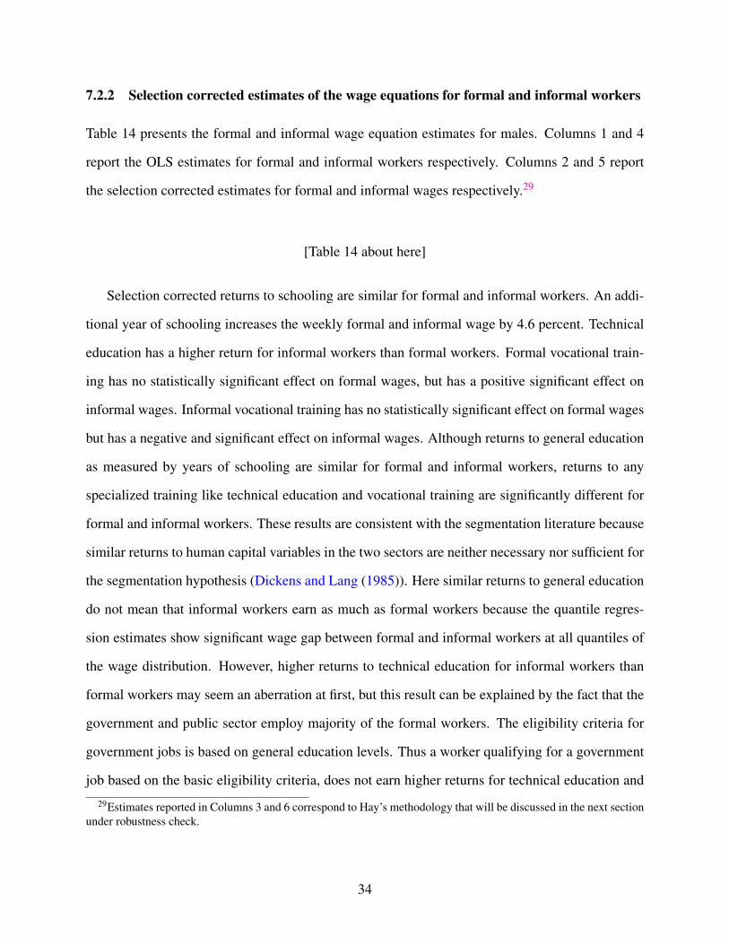
7.2.2 Selection corrected estimates of the wage equations for formal and informal workers

Table 14 presents the formal and informal wage equation estimates for males. Columns 1 and 4

report the OLS estimates for formal and informal workers respectively. Columns 2 and 5 report

the selection corrected estimates for formal and informal wages respectively.29

[Table 14 about here]

Selection corrected returns to schooling are similar for formal and informal workers. An addi-

tional year of schooling increases the weekly formal and informal wage by 4.6 percent. Technical

education has a higher return for informal workers than formal workers. Formal vocational train-

ing has no statistically significant effect on formal wages, but has a positive significant effect on

informal wages. Informal vocational training has no statistically significant effect on formal wages

but has a negative and significant effect on informal wages. Although returns to general education

as measured by years of schooling are similar for formal and informal workers, returns to any

specialized training like technical education and vocational training are significantly different for

formal and informal workers. These results are consistent with the segmentation literature because

similar returns to human capital variables in the two sectors are neither necessary nor sufficient for

the segmentation hypothesis (Dickens and Lang (1985)). Here similar returns to general education

do not mean that informal workers earn as much as formal workers because the quantile regres-

sion estimates show significant wage gap between formal and informal workers at all quantiles of

the wage distribution. However, higher returns to technical education for informal workers than

formal workers may seem an aberration at first, but this result can be explained by the fact that the

government and public sector employ majority of the formal workers. The eligibility criteria for

government jobs is based on general education levels. Thus a worker qualifying for a government

job based on the basic eligibility criteria, does not earn higher returns for technical education and

29Estimates reported in Columns 3 and 6 correspond to Hay’s methodology that will be discussed in the next sectionunder robustness check.

34

vocational training.30 Returns to experience (measured by age) are almost the same for formal and

informal workers.

Religion does not play a significant role in determining the formal wage, but is important for the

informal wage. Scheduled castes and other backward classes face wage penalties for both formal

and informal workers compared to other higher castes. Marital status does not have any significant

effect on the formal wage. But married informal workers earn 15 percent more compared to un-

married informal workers. Formal workers located in the urban regions earn 14 percent more than

formal workers located in the rural regions. Informal workers located in the urban region earn 10.2

percent more than informal workers located in rural regions.

Table 15 reports the formal and informal wage estimates for female workers. As in Table 14,

columns 1 and 4 report the OLS estimates for formal and informal wages respectively. Columns 2

and 5 report the selection corrected estimates for formal and informal wages respectively.31

[Table 15 about here]

Selection corrected returns to schooling has no significant effect on the formal wage. However,

returns to schooling for informal workers are 6.7 percent. Technical education has no significant

effect on formal workers but has positive and significant returns for informal workers. Formal

vocational training has a negative premium attached with respect to formal wage while it has no

significant effect on informal wage. The same argument follows as with men that the government

jobs cover majority of formal employment, where the minimum eligibility criteria is based on

general education levels. The negative premium on formal vocational training for formal workers

30Duraisamy (2002) estimated returns to education for workers in wage employment using NSSO data for the years1983 and 1993. He finds that men receive 6.4 percent, 15.7 percent and 8.9 percent returns on middle, secondary andhigher secondary levels. Women received 10.3 percent , 33.7 percent and 11.8 percent returns for the same levels ofeducation. Azam (2012) used NSSO data for the years 1983, 1993 and 2004 to estimate the returns to education. Heuses quantile regression techniques and finds that returns to education have increased during the period 1983-2004.Both the studies do not make a distinction between formal and informal workers. The estimates reported in this paperare slightly different from the earlier studies because, I use years of schooling as a measure of education and they usedummy variables for each level of education.

31As in table 14, estimates reported in Columns 3 and 6 correspond to Hay’s methodology that will be discussed inthe next section under robustness check.

35

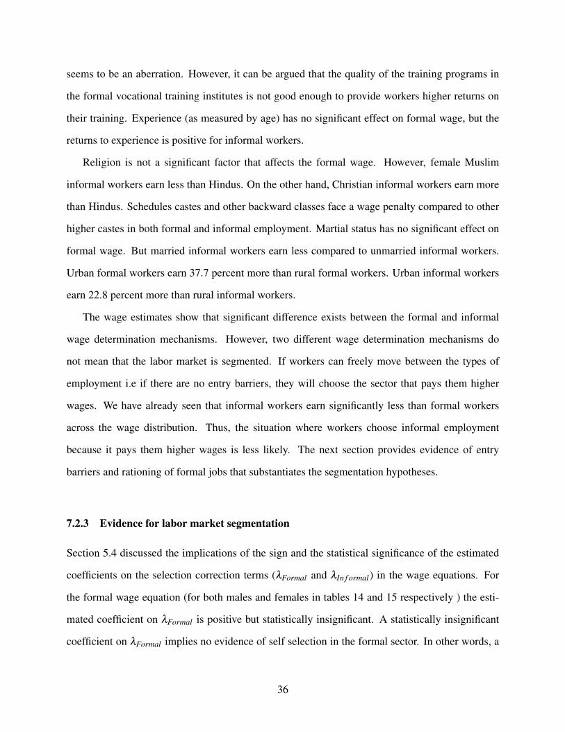
seems to be an aberration. However, it can be argued that the quality of the training programs in

the formal vocational training institutes is not good enough to provide workers higher returns on

their training. Experience (as measured by age) has no significant effect on formal wage, but the

returns to experience is positive for informal workers.

Religion is not a significant factor that affects the formal wage. However, female Muslim

informal workers earn less than Hindus. On the other hand, Christian informal workers earn more

than Hindus. Schedules castes and other backward classes face a wage penalty compared to other

higher castes in both formal and informal employment. Martial status has no significant effect on

formal wage. But married informal workers earn less compared to unmarried informal workers.

Urban formal workers earn 37.7 percent more than rural formal workers. Urban informal workers

earn 22.8 percent more than rural informal workers.

The wage estimates show that significant difference exists between the formal and informal

wage determination mechanisms. However, two different wage determination mechanisms do

not mean that the labor market is segmented. If workers can freely move between the types of

employment i.e if there are no entry barriers, they will choose the sector that pays them higher

wages. We have already seen that informal workers earn significantly less than formal workers

across the wage distribution. Thus, the situation where workers choose informal employment

because it pays them higher wages is less likely. The next section provides evidence of entry

barriers and rationing of formal jobs that substantiates the segmentation hypotheses.

7.2.3 Evidence for labor market segmentation

Section 5.4 discussed the implications of the sign and the statistical significance of the estimated

coefficients on the selection correction terms (λFormal and λIn f ormal) in the wage equations. For

the formal wage equation (for both males and females in tables 14 and 15 respectively ) the esti-

mated coefficient on λFormal is positive but statistically insignificant. A statistically insignificant

coefficient on λFormal implies no evidence of self selection in the formal sector. In other words, a

36

worker’s unobserved productivity that increases his chances of formal employment does not affect

his wages. Also there is no difference between a randomly selected formal worker and a worker

who self selects into formal employment. No evidence of self selection into formal employment

insinuates to the fact that entry barriers may be present in the formal sector. However, it could also

be the case that the model is not identified properly that would require some further testing of the

model with alternative identification strategies. Decomposition of the wage gap into characteristics

and coefficient effects may give further insights to labor market segmentation hypothesis. I discuss

the results in the next section.

The coefficient on λIn f ormal is negative and statistically significant. A negative coefficient on

λIn f ormal implies that informal employment is a competitive choice for the worker. Workers can

self select into informal employment and increase the informal wage. Also, a worker self selecting

into informal employment earns higher wages than a randomly selected informal worker.

Based on these two findings we cannot reject the hypothesis that the labor market is segmented.

This is because there is no evidence of self selection into formal employment. If on the contrary we

had found that workers can self select into both formal and informal employment we could have

safely rejected the labor market segmentation hypothesis. Since in that case, the workers would

be free to choose between formal and informal employment. They would choose the sector that

maximizes his utility. Decomposition of the wage gap into coefficient and characteristic effect may

provide further insights to this argument. However, I have to constrain myself to the decomposition

at the mean. The underlying self selection model is a polychotomous choice model that does not

allow the implementation of the MM decomposition technique across the quantiles of the wage

distribution. I have used the Oaxaca-Blinder technique to decompose the formal-informal wage

gap into coefficient and characteristics effect.

37

7.2.4 Wage gap decomposition adjusting for self selection (Oaxaca-Blinder)

Table 16 shows the wage gap decomposition into coefficient and and endowment effects. The

first column shows the results for males and the second column for females. For both males and

females, the formal-informal wage gap is higher when corrected for self selection. For males, the

coefficient effect explains 66 percent of the wage gap and the endowment effect explains the rest

34 percent. For females, the coefficient effects explain 84 percent of the formal informal wage gap.

So, at the mean, the informal workers face a wage penalty because they receive lower returns on

their human capital and individual characteristics. So formal workers enjoy higher returns on their

human capital and individual characteristics. This finding is compatible with the efficiency wage

theory in the sense that firms pay higher wages to formal workers that is set higher than than the

market clearing wage to incentivize the worker. So, formal workers who receive higher returns to

their skills and individual characteristics have less incentivize to move elsewhere. On average they

could also be more productive than the informal workers because they receive higher returns.

A significant part of the wage gap is explained by the differences in characteristics of the formal

and informal workers. These differences may stem from skill differences, age and other individual

characteristics. So, if workers with different characteristics have different labor supply elasticities,

firms can exploit to opportunity to exercise their monopsonistic power. This line of argument is

also compatible with labor market segmentation because firms having monopsonistic power can

now pay different wages to the workers with different labor supply elasticities. In our case, it may

be optimal for the firms to pay different wage to formal and informal workers because they have

differ in skills and individual characteristics and hence have different labor supply elasticities.

Figures 2 and 3 are the kernel density plots of the predicted formal wage and the observed

informal wage for the informal male workers and informal female workers respectively. The coun-

terfactual is based on the differences in returns to human capital and individual characteristics.

That is, how much the informal workers would have earned if they had received similar returns

on human capital and individual characteristics as the formal workers. For males, we see that pre-

dicted mean and median formal wage is higher than the observed informal wage. Also, 85 percent

38

of the male informal workers (83 percent of female informal workers) would have earned higher

wages in formal employment than their observed informal wage. Given that informal workers do

not receive any non-wage benefits as formal workers, the result shows the majority of the informal

workers would choose formal employment over informal employment.The other 15 percent of the

male informal workers (17 percent of the female informal workers) would have earned less as for-

mal workers. These few people could be regarded as voluntary informal workers who would have

chosen informal employment even if they had full access to formal employment. No discernible

differences in observed characteristics can be found between the involuntary informal workers and

the voluntary informal workers. But majority of the voluntary informal workers are employed by

the proprietary and the government enterprises. So, it could be the case that these enterprises pay

a higher wage to informal workers instead of providing defined employment benefits to the work-

ers. These individuals could also posses entrepreneurial skills that are rewarded by the proprietary

enterprises that compensates for the employment benefits that accompany formal employment.

[Figures 2 and 3 about here]

7.2.5 Robustness check

I conducted the robustness check for my results by employing the selection correction strategy

proposed by Hay (1980). This methodology imposes stronger restrictions on the model by as-

suming linearity of the conditional expectation of the error terms in the wage equation conditional

on the errors in the selection equation. But the results should not be different from our baseline

model. The selection correction terms constructed from the first stage multinomial logit estimates

are given by equation 14 in section 6.2. Columns 3 and 6 in Table 14 and 15 report the wage esti-

mates employing Hay’s method. For both males and females, the results are similar to the baseline

model. The coefficients on λFormalHay are statistically insignificant that provides evidence for entry

barriers in the formal employment. The coefficients on λIn f ormalHay are negative and significant that

implies informal employment is a competitive outcome given that workers cannot self select into

formal employment. Moreover, the coefficient estimates from both models are almost the same.

39

Thus, the results presented in this paper are robust and invariant to the other polychotomous choice

models used in the literature.

8 Conclusions

The results in this paper show that the Indian labor market is segmented between formal and in-

formal employment. Evidence does not support the hypothesis of a fully competitive labor market

and that workers choose informal employment as the last resort. This finding is in strong contrast

to the empirical evidence from some Latin American countries that show informal employment

is a competitive choice for workers over formal employment. The paper shows that majority of

the workers would have earned more as formal workers than their current informal wage if they

had full access to formal employment. Also, informal workers earn significantly less than formal

workers as reflected by the wage gap between the two sets of workers at all quantiles of the wage

distribution. Thus, the finding refutes the hypothesis of voluntary informal employment for ma-

jority of the workers. The current empirical and theoretical literature on informal employment is

mainly based on Latin American countries. Evidence amassed in this paper show that the Indian

labor market is systematically different from Latin American countries providing the platform for

further research on both empirical and theoretical grounds focusing on South Asian countries.

The wage gap decomposition results show that both coefficient and endowment effects explain

significant portion of the formal-informal wage gap at all quantiles of the wage distribution. This

evidence suggests that informal workers earn less than formal workers not only because they have

different endowments, but also because they face discrimination in terms of lower returns to their

endowments than their formal counterparts. Recent policies focus on skill development to address

the problem of informal employment. However, policies should also address the problem of dis-

crimination faced by informal workers as firms pay lower returns to their skills and characteristics.

Moreover, results also show that workers having technical education and vocational training do

40

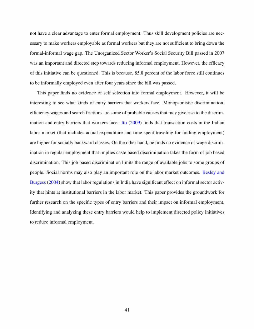
not have a clear advantage to enter formal employment. Thus skill development policies are nec-

essary to make workers employable as formal workers but they are not sufficient to bring down the

formal-informal wage gap. The Unorganized Sector Worker’s Social Security Bill passed in 2007

was an important and directed step towards reducing informal employment. However, the efficacy

of this initiative can be questioned. This is because, 85.8 percent of the labor force still continues

to be informally employed even after four years since the bill was passed.

This paper finds no evidence of self selection into formal employment. However, it will be

interesting to see what kinds of entry barriers that workers face. Monopsonistic discrimination,

efficiency wages and search frictions are some of probable causes that may give rise to the discrim-

ination and entry barriers that workers face. Ito (2009) finds that transaction costs in the Indian

labor market (that includes actual expenditure and time spent traveling for finding employment)

are higher for socially backward classes. On the other hand, he finds no evidence of wage discrim-

ination in regular employment that implies caste based discrimination takes the form of job based

discrimination. This job based discrimination limits the range of available jobs to some groups of

people. Social norms may also play an important role on the labor market outcomes. Besley and

Burgess (2004) show that labor regulations in India have significant effect on informal sector activ-

ity that hints at institutional barriers in the labor market. This paper provides the groundwork for

further research on the specific types of entry barriers and their impact on informal employment.

Identifying and analyzing these entry barriers would help to implement directed policy initiatives

to reduce informal employment.

41

Figures

Figure 1: Share of informal employment in the non agricultural sector, by countries

Source: ILO (2013)32

Figure 2 : Predicted formal wage for informal workers (Males)

Figure 3 : Predicted formal wage for informal workers (Females)

32The figures represent the latest data available for each country.

42

Tables

Table 1: Classification of informal employment and informal sectorProduction Units Informal jobs Formal Jobs

Informal sector enterprises A BOther units of production C D

A+C = Persons in Informal Employment

A+B = Persons Employed in the Informal Sector

C = Informal Employment outside the Informal Sector

B = Formal Employment in the Informal Sector

Table 2 : Identification of formal/informal sector, by type of enterpriseEnterprise type Frequency %Informal sector1. Proprietary (male) 55702 62.32. Proprietary (female) 4318 4.73. Partnership (members from same hh) 1833 1.94. Partnership (with members from different hh) 1265 1.68. Employer’s households(i.e., private households) 1290 1.69 . Others 4826 5.3Formal sector5. Government/public sector 18591 12.86. Public/Private limited company 5902 8.57. Co-operative societies/trusts 1198 1.2Total 94639 100.0Source: Author’s calculation based on NSSO 68th Round Employment-Unemployment data

Table 3 : Identifying broad categories of employment, by principal activity statusPrincipal activity status Frequency %Self employed1. Self-employed (own account worker) 30807 11.52. Self-employed (Employer) 1320 0.53. Self-employed (unpaid family member) 7232 2.6Employees4. Regular salaried/ wage employee 37329 14.45. Casual wage labor (public works) 902 0.46. Casual wage labor (other types) 17219 8.5Not in the labor force7. Did not work but was seeking for work 5508 1.98.Attended educational institution 42415 18.59. Attended domestic duties only 48902 21.910. Attended domestic duties & other activities 33378 18.311. Rentiers, pensioners, remittance recipients 1263 0.612. Others (begging, prostitution,etc.) 1564 0.8Total 227839 100Source: Author’s calculation based on NSSO 68th Round Employment-Unemployment data

43

Table 4 : Percentage of workers receiving employment benefitsEmployment benefits Social security Job contract Paid leave All benefits

% % % %No 69.4 77.1 32.0 82.6Yes 30.6 22.9 68.0 17.4Total 100 100 100 100Observations 55,450Source: Author’s calculation based on NSSO 68th Round Employment-Unemployment data

Table 5: Formal and informal employment (treating self employed as a separate category)Male Female All

Categories Frequency % Frequency % Frequency %Formal employment 11087 7.4 2377 1.3 13464 4.1Informal employment 34921 35.9 7065 5.6 41986 19.3Self employed 33307 27.3 6052 4.3 39359 14.7Not in labor force 29904 29.4 103126 88.8 133030 62.0Total 109219 100.0 118620 100.0 227839 100.0Source: Author’s calculation based on NSSO 68th Round Employment-Unemployment data

Table 6: Identification of formal and informal sector and employment based on enterprise type and activity status

Self employed

Own account worker Employers Contributing family members Employees

(Activity Status:1) (Activity Status:2) (Activity Status:3) (Activity Status:4,5,6)

Formal Informal Formal Informal Informal Formal Informal

Formal sector A NE B NE C D E

(Enterprise types :5,6,7)

Informal sector NE F NE G H I J

(Enterprise types :1,2,3,4,8,9)

Source:Sastry (2004) and own calculation

Table 7 : Formal and informal employment in the formal and informal sectorsEmployment type, by sector Frequency %Formal employment1. Formal employment in formal sector (A+B+D) 12770 4.43. Formal employment in informal sector (I) 737 0.1Informal employment2. Informal employment in formal sector (C+E) 12797 8.74. Informal employment in informal sector (F+G+H+I+J) 68505 24.85. Not in labor force 133030 62.0Total 227839 100.0Source: Author’s calculation based on NSSO 68th Round Employment-Unemployment data

44

Table 8: Summary statistics all covariates (Males)

Formal Informal Self employed Not in labor force

mean sd mean sd mean sd mean sd

Wages and Consumption

Weekly Wage (Rupees) 4966.4 3363.4 1771.4 1889.2 . . . .

Log weekly wage (Rupees) 8.3 0.6 7.2 0.7 . . . .

MPCE (Rupees) 2902.5 2621.5 1714.4 1420.8 1806.4 1585.1 1970.2 1859.1

Log MPCE 7.8 0.6 7.3 0.6 7.3 0.6 7.4 0.6

Age 42.1 9.6 34.2 10.5 37.2 10.3 20.1 7.4

Education

Years of Schooling 12.5 4.0 7.4 5.2 8.0 4.9 10.1 3.2

Technical education 0.2 0.4 0.05 0.2 0.03 0.2 0.04 0.2

No vocational training 0.8 0.4 0.8 0.4 0.8 0.4 0.9 0.2

Vocational training: formal 0.1 0.3 0.05 0.2 0.04 0.2 0.05 0.2

Vocational training: informal 0.07 0.3 0.2 0.4 0.2 0.4 0.01 0.1

Dependents

No of Children in the hhd (<15 years) 1.1 1.2 1.3 1.4 1.5 1.5 0.9 1.3

No. of elders (>60 years) 0.2 0.5 0.2 0.5 0.3 0.6 0.3 0.5

Caste

Scheduled tribe 0.06 0.2 0.06 0.2 0.03 0.2 0.07 0.3

Scheduled caste 0.1 0.4 0.2 0.4 0.1 0.3 0.2 0.4

Other backward class 0.3 0.5 0.4 0.5 0.4 0.5 0.4 0.5

Others 0.5 0.5 0.3 0.5 0.4 0.5 0.3 0.5

Marital status

Never married 0.1 0.3 0.3 0.4 0.2 0.4 0.9 0.3

Currently married 0.9 0.3 0.7 0.5 0.8 0.4 0.06 0.2

Widowed 0.009 0.10 0.01 0.1 0.01 0.1 0.005 0.07

Divorced/separated 0.002 0.04 0.004 0.06 0.002 0.05 0.0009 0.03

Regional variables

Urban 0.7 0.5 0.5 0.5 0.5 0.5 0.4 0.5

North 0.2 0.4 0.2 0.4 0.3 0.4 0.3 0.4

West 0.3 0.4 0.2 0.4 0.2 0.4 0.2 0.4

East 0.2 0.4 0.2 0.4 0.2 0.4 0.2 0.4

North-East 0.03 0.2 0.03 0.2 0.04 0.2 0.04 0.2

Central 0.07 0.3 0.06 0.2 0.06 0.2 0.07 0.3

South 0.2 0.4 0.3 0.4 0.2 0.4 0.2 0.4

Observations 109219

Notes: The summary statistics for religion dummies are not reported in this table due space constraint.

See section 5.2.2 for the discussion on the distribution of religious groups.

45

Table 9: Summary statistics all covariates (Females)

Formal Informal Self employed Not in labor force

mean sd mean sd mean sd mean sd

Wages and Consumption

Weekly Wage (Rupees) 4330.9 2956.7 1367.6 1741.4 . . . .

Log weekly wage (Rupees) 8.1 0.8 6.8 0.9 . . . .

MPCE (Rupees) 3651.7 3559.2 2007.2 2164.2 1756.4 1599.2 1794.4 1662.4

Log MPCE 8.0 0.7 7.4 0.6 7.3 0.6 7.3 0.6

Age 39.0 9.9 34.9 10.4 36.2 10.8 32.0 12.1

Education

Years of Schooling 13.0 4.1 7.3 6.2 5.6 5.1 6.7 5.1

Technical education 0.2 0.4 0.06 0.2 0.03 0.2 0.01 0.1

No vocational training 0.8 0.4 0.8 0.4 0.7 0.5 1.0 0.2

Vocational training: formal 0.2 0.4 0.07 0.3 0.06 0.2 0.02 0.1

Vocational training: informal 0.04 0.2 0.09 0.3 0.2 0.4 0.03 0.2

Dependents

No of Children in the hhd (<15 years) 1.0 1.1 1.1 1.3 1.3 1.3 1.4 1.5

No. of elders (>60 years) 0.4 0.6 0.2 0.5 0.2 0.5 0.3 0.6

Caste

Scheduled tribe 0.06 0.2 0.09 0.3 0.05 0.2 0.06 0.2

Scheduled caste 0.1 0.4 0.2 0.4 0.2 0.4 0.2 0.4

Other backward class 0.3 0.5 0.4 0.5 0.5 0.5 0.4 0.5

Others 0.5 0.5 0.3 0.4 0.3 0.5 0.3 0.5

Marital status

Never married 0.2 0.4 0.2 0.4 0.2 0.4 0.2 0.4

Currently married 0.7 0.5 0.6 0.5 0.7 0.5 0.7 0.4

Widowed 0.2 0.4 0.1 0.4 0.1 0.3 0.03 0.2

Divorced/separated 0.02 0.1 0.03 0.2 0.02 0.1 0.003 0.05

Regional variables

Urban 0.7 0.5 0.5 0.5 0.5 0.5 0.3 0.5

North 0.2 0.4 0.1 0.3 0.1 0.4 0.3 0.4

West 0.3 0.4 0.2 0.4 0.2 0.4 0.2 0.4

East 0.2 0.4 0.1 0.3 0.2 0.4 0.2 0.4

North-East 0.03 0.2 0.02 0.1 0.03 0.2 0.04 0.2

Central 0.05 0.2 0.07 0.3 0.05 0.2 0.07 0.3

South 0.3 0.5 0.4 0.5 0.4 0.5 0.2 0.4

Observations 118620

Notes: The summary statistics for religion dummies are not reported in this table due space constraint.

See section 5.2.2 for the discussion on the distribution of religious groups.

46

Table 10: Wage gap decomposition (Males)

Quantiles Wage gap (raw) Wage gap (predicted) Endowment effect Coefficient effect

10 -1.101 -1.155 -0.536 -0.619

(0.025) (0.024) (0.034)

20 -1.299 -1.245 -0.592 -0.652

(0.018) (0.022) (0.028)

30 -1.338 -1.278 -0.638 -0.640

(0.015) (0.022) (0.027)

40 -1.325 -1.284 -0.673 -0.611

(0.014) (0.022) (0.026)

50 -1.288 -1.267 -0.692 -0.574

(0.015) (0.021) (0.025)

60 -1.273 -1.229 -0.693 -0.536

(0.015) (0.020) (0.025)

70 -1.247 -1.169 -0.672 -0.497

(0.016) (0.021) (0.027)

80 -1.170 -1.077 -0.632 -0.445

(0.010) (0.022) (0.029)

90 -0.788 -0.929 -0.558 -0.372

(0.024) (0.025) (0.034)

Observations 46008

Table 11: Wage gap decomposition (Females)

Quantiles Wage gap (raw) Wage gap (predicted) Endowment effect Coefficient effect

10 -1.153 -1.278 -0.668 -0.610

(0.032) (0.028) (0.043)

20 -1.440 -1.431 -0.713 -0.718

(0.027) (0.026) (0.0381)

30 -1.579 -1.520 -0.749 -0.771

(0.022) (0.026) (0.035)

40 -1.573 -1.549 -0.786 -0.763

(0.019) (0.026) (0.033)

50 -1.661 -1.543 -0.814 -0.728

(0.019) (0.026) (0.033)

60 -1.545 -1.497 -0.813 -0.684

(0.019) (0.026) (0.0317)

70 -1.453 -1.413 -0.775 -0.638

(0.021) (0.026) (0.033)

80 -1.342 -1.277 -0.688 -0.589

(0.023) (0.026) (0.034)

90 -0.823 -1.049 -0.551 -0.497

(0.028) (0.028) (0.040)

Observations 9442

47

Table 12: Multinomial logit estimates of the sectoral allocation equations (Males)Coefficient Estimates Marginal effects

Informal Self employed Not in labor force Formal Informal Self employed Not in labor forceEducationYears of Schooling -0.251∗∗∗ -0.214∗∗∗ -0.000 0.0111 -0.0232 -0.0046 0.0166

(0.003) (0.003) (0.005)Technical education -0.123∗∗ -0.567∗∗∗ -0.585∗∗∗ 0.0197 0.0928 -0.0914 -0.0211

(0.045) (0.047) (0.060)Vocational training: formal -0.334∗∗∗ -0.419∗∗∗ -0.398∗∗∗ 0.0237 0.0066 -0.0277 -0.0026

(0.047) (0.048) (0.060)Vocational training: informal 0.275∗∗∗ 0.631∗∗∗ -2.100∗∗∗ -0.0149 -0.0207 0.1336 -0.0980

(0.044) (0.043) (0.077)Age -0.135∗∗∗ -0.099∗∗∗ -0.967∗∗∗ 0.0104 0.0224 0.0325 -0.0653

(0.011) (0.011) (0.013)Age2 0.001∗∗∗ 0.001∗∗∗ 0.011∗∗∗ -0.0001 -0.0004 -0.0004 0.0008

(0.000) (0.000) (0.000)DependentsNo of Children (<15 years) 0.072∗∗∗ 0.142∗∗∗ 0.065∗∗∗ -0.0051 -0.0107 0.0183 -0.0025

(0.011) (0.010) (0.014)No. of elders (>60 years) 0.022 0.178∗∗∗ 0.283∗∗∗ -0.0056 -0.0386 0.0286 0.0156

(0.023) (0.022) (0.029)CasteScheduled tribe -0.516∗∗∗ -1.136∗∗∗ -0.609∗∗∗ 0.0526 0.0871 -0.1491 0.0094

(0.048) (0.049) (0.064)Scheduled caste -0.043 -0.713∗∗∗ -0.380∗∗∗ 0.0182 0.1292 -0.1410 -0.0063

(0.040) (0.041) (0.052)Other backward class 0.089∗∗ 0.048 -0.014 -0.0031 0.0138 -0.0046 -0.0061

(0.031) (0.030) (0.039)Marital statusCurrently married -0.215∗∗∗ -0.025 -1.657∗∗∗ -0.0150 -0.0301 -0.0946 0.1398

(0.050) (0.050) (0.059)Widowed -0.178 -0.183 0.424∗∗ -0.0196 -0.157 -0.1716 0.3419

(0.135) (0.135) (0.157)Divorced/separated -0.050 -0.091 0.484 -0.0230 -0.1352 -0.1690 0.3272

(0.231) (0.234) (0.282)Regional VariablesUrban 0.138∗∗∗ 0.082∗∗ -0.159∗∗∗ -0.0089 0.0272 0.0077 -0.0260

(0.026) (0.025) (0.032)Regional dummies Yes Yes YesReligion dummies Yes Yes YesConstant 8.512∗∗∗ 6.515∗∗∗ 19.582∗∗∗

(0.207) (0.207) (0.224)χ2 110089.51 8727.92 14897.18Log likelihood -93745.166

N 109219∗ p < 0.05 , ∗∗ p < 0.01 , ∗∗∗ p < 0.001Notes : The reference category is formal employment.Omitted category for Vocational training is ‘No vocational training’,for Caste is ‘others’ (that includes higher castes) and for Marital status is ‘never married’.Coefficients on religion dummies are not reported due to space constraint.χ2 is the test statistic for the null hypothesis that coefficients are jointly equal to zero.

48

Table 13: Multinomial logit estimates of the sectoral allocation equations (Females)Coefficient estimates Marginal Effects

Informal Self employed Not in labor force Formal Informal Self employed Not in Labor forceEducationYears of Schooling -0.319∗∗∗ -0.381∗∗∗ -0.327∗∗∗ 0.0013 0.0004 -0.0019 0.0001

(0.007) (0.007) (0.007)Technical education -0.034 -0.770∗∗∗ -1.085∗∗∗ 0.0064 0.0653 0.0088 -0.0805

(0.087) (0.116) (0.075)Vocational training: formal -0.140 0.424∗∗∗ -0.978∗∗∗ 0.0049 0.0385 0.0830 -0.1265

(0.084) (0.093) (0.074)Vocational training: informal 0.419∗∗∗ 1.629∗∗∗ -0.789∗∗∗ 0.0022 0.0499 0.2144 -0.2664

(0.120) (0.117) (0.114)Age -0.027 -0.128∗∗∗ -0.438∗∗∗ 0.0016 0.0157 0.0098 -0.0270

(0.021) (0.021) (0.019)Age2 -0.001∗ 0.001∗∗ 0.005∗∗∗ 0.0000 -0.0002 -0.0001 0.0003

(0.000) (0.000) (0.000)DependentsNo. of Children (<15 years) 0.021 0.043 0.071∗∗ -0.0002 -0.0019 -0.0009 0.0030

(0.023) (0.024) (0.021)No. of elders (>60 years) -0.088∗ -0.003 0.005 0.0000 -0.0037 -0.0001 0.0038

(0.043) (0.044) (0.037)CasteScheduled tribe -0.362∗∗∗ -0.840∗∗∗ -0.991∗∗∗ 0.0052 0.0290 0.0035 -0.0377

(0.098) (0.102) (0.088)Scheduled caste -0.079 -0.551∗∗∗ -0.639∗∗∗ 0.0029 0.0263 0.0018 -0.0309

(0.086) (0.092) (0.080)Other backward class 0.045 0.234∗∗∗ 0.022 -0.0002 0.0005 0.0073 -0.0076

(0.066) (0.067) (0.059)Marital statusCurrently married -0.653∗∗∗ -0.389∗∗∗ 0.628∗∗∗ -0.0020 -0.0645 -0.0393 0.1060

(0.095) (0.100) (0.087)Widowed -0.784∗∗∗ -1.106∗∗∗ -1.632∗∗∗ 0.0134 0.0451 0.0189 -0.0774

(0.123) (0.130) (0.114)Divorced/separated -0.119 -0.585∗∗ -1.099∗∗∗ 0.0066 0.0583 0.0183 -0.0832

(0.208) (0.224) (0.203)Regional VariablesUrban 0.599∗∗∗ 0.407∗∗∗ 0.174∗∗∗ -0.0008 0.0185 0.0086 -0.0263

(0.054) (0.055) (0.049)Regional dummies Yes Yes YesReligion dummies Yes Yes YesConstant 7.166∗∗∗ 8.644∗∗∗ 15.978∗∗∗

(0.373) (0.379) (0.347)χ2 2904.47 3777.8 5075.33Log likelihood -51015.008

N 118620∗ p < 0.05 , ∗∗ p < 0.01 , ∗∗∗ p < 0.001Notes : The reference category is formal employment.Omitted category for Vocational training is ‘No vocational training’,for Caste is ‘others’ (that includes higher castes) and for Marital status is ‘never married’.Coefficients on religion dummies are not reported due to space constraint.χ2 is the test statistic for the null hypothesis that coefficients are jointly equal to zero.

49

Table 14: Selection corrected wage estimates for formal and informal workers (Males)(1) (2) (3) (4) (5) (6)

Formal InformalEducation OLS Selection (Lee) Selection (Hay) OLS Selection (Lee) Selection (Hay)

Years of Schooling 0.054∗∗∗ 0.046∗∗∗ 0.062∗∗∗ 0.050∗∗∗ 0.046∗∗∗ 0.044∗∗∗

(0.002) (0.006) (0.004) (0.001) (0.001) (0.001)Technical education 0.207∗∗∗ 0.191∗∗∗ 0.217∗∗∗ 0.313∗∗∗ 0.321∗∗∗ 0.325∗∗∗

(0.017) (0.020) (0.018) (0.021) (0.021) (0.021)Vocational training: formal 0.038∗ 0.022 0.050∗∗ 0.042∗ 0.042∗ 0.042∗∗

(0.017) (0.019) (0.019) (0.017) (0.017) (0.016)Vocational training: informal 0.003 0.017 -0.010 -0.031∗∗∗ -0.028∗∗∗ -0.025∗∗

(0.021) (0.024) (0.022) (0.009) (0.009) (0.009)Age 0.042∗∗∗ 0.033∗∗∗ 0.051∗∗∗ 0.025∗∗∗ 0.032∗∗∗ 0.036∗∗∗

(0.005) (0.008) (0.007) (0.002) (0.003) (0.003)Age2 -0.000∗∗∗ -0.000∗ -0.000∗∗∗ -0.000∗∗∗ -0.000∗∗∗ -0.000∗∗∗

(0.000) (0.000) (0.000) (0.000) (0.000) (0.000)CasteScheduled tribe -0.020 -0.052 0.006 -0.023 -0.009 -0.005

(0.019) (0.027) (0.024) (0.013) (0.013) (0.013)Scheduled caste -0.094∗∗∗ -0.108∗∗∗ -0.082∗∗∗ -0.110∗∗∗ -0.089∗∗∗ -0.083∗∗∗

(0.017) (0.019) (0.018) (0.010) (0.011) (0.011)Other backward class -0.069∗∗∗ -0.066∗∗∗ -0.071∗∗∗ -0.095∗∗∗ -0.093∗∗∗ -0.092∗∗∗

(0.013) (0.013) (0.014) (0.009) (0.009) (0.009)Marital StatusCurrently married 0.061∗ 0.045 0.077∗∗ 0.140∗∗∗ 0.149∗∗∗ 0.152∗∗∗

(0.025) (0.027) (0.027) (0.010) (0.010) (0.010)Widowed 0.060 0.060 0.063 -0.046 -0.035 -0.032

(0.063) (0.064) (0.065) (0.035) (0.033) (0.035)Divorced/separated 0.147 0.140 0.156 -0.089 -0.080 -0.078

(0.112) (0.117) (0.116) (0.049) (0.049) (0.049)Regional VariablesUrban 0.139∗∗∗ 0.140∗∗∗ 0.137∗∗∗ 0.096∗∗∗ 0.102∗∗∗ 0.104∗∗∗

(0.011) (0.011) (0.010) (0.007) (0.007) (0.007)Regional dummies Yes Yes Yes Yes Yes YesReligion dummies Yes Yes Yes Yes Yes YesSelection Correction termsλFormal 0.097

(0.060)λFormalHay -0.099

(0.056)λIn f ormal -0.107∗∗∗

(0.019)λIn f ormalHay -0.231∗∗∗

(0.026)Constant 6.115∗∗∗ 6.627∗∗∗ 5.699∗∗∗ 6.106∗∗∗ 5.934∗∗∗ 5.881∗∗∗

(0.109) (0.328) (0.250) (0.041) (0.052) (0.048)

N 11087 11087 11087 34921 34921 34921

R2 0.278 0.278 0.278 0.326 0.326 0.327∗ p < 0.05 , ∗∗ p < 0.01 , ∗∗∗ p < 0.001 . Bootstrap standard errors in parenthesis.Notes : Omitted category for Vocational training is ‘No vocational training’,for Caste is ‘others’ (that includes higher castes) and for Marital status is ‘never married’.Coefficients of religion dummies are not reported due to space constraint.

50

Table 15: Selection corrected wage estimates for formal and informal workers (Females)(1) (2) (3) (4) (5) (6)

Formal InformalEducation OLS Selection (Lee) Selection (Hay) OLS Selection (Lee) Selection (Hay)

Years of Schooling 0.081∗∗∗ 0.033 0.036 0.067∗∗∗ 0.066∗∗∗ 0.067∗∗∗

(0.004) (0.025) (0.021) (0.002) (0.002) (0.002)Technical education 0.205∗∗∗ 0.064 0.100 0.348∗∗∗ 0.567∗∗∗ 0.528∗∗∗

(0.037) (0.076) (0.061) (0.040) (0.054) (0.052)Vocational training: formal -0.048 -0.159∗ -0.140∗ -0.070 0.083 0.061

(0.040) (0.073) (0.060) (0.038) (0.049) (0.046)Vocational training: informal -0.131 -0.159∗ -0.161∗ -0.041 0.136∗∗ 0.113∗

(0.071) (0.073) (0.071) (0.031) (0.043) (0.044)Age 0.028∗ -0.026 -0.021 0.029∗∗∗ 0.119∗∗∗ 0.112∗∗∗

(0.012) (0.029) (0.025) (0.007) (0.018) (0.017)Age2 -0.000 0.001 0.000 -0.000∗ -0.001∗∗∗ -0.001∗∗∗

(0.000) (0.000) (0.000) (0.000) (0.000) (0.000)CasteScheduled tribe 0.059 -0.074 -0.057 0.130∗∗∗ 0.270∗∗∗ 0.252∗∗∗

(0.051) (0.084) (0.075) (0.033) (0.041) (0.040)Scheduled caste -0.127∗ -0.206∗∗ -0.194∗∗ -0.058∗ 0.074 0.059

(0.052) (0.064) (0.059) (0.027) (0.038) (0.035)Other backward class -0.159∗∗∗ -0.152∗∗∗ -0.154∗∗∗ -0.103∗∗∗ -0.103∗∗∗ -0.103∗∗∗

(0.038) (0.038) (0.038) (0.025) (0.025) (0.025)Marital statusCurrently married -0.008 0.057 0.054 0.090∗∗ -0.213∗∗∗ -0.185∗∗

(0.047) (0.053) (0.053) (0.029) (0.062) (0.059)Widowed 0.091 -0.107 -0.062 0.068 0.231∗∗∗ 0.179∗∗∗

(0.059) (0.118) (0.093) (0.038) (0.052) (0.043)Divorced/separated 0.003 -0.097 -0.076 -0.032 0.153∗ 0.090

(0.105) (0.119) (0.114) (0.053) (0.065) (0.057)Regional VariablesUrban 0.341∗∗∗ 0.377∗∗∗ 0.371∗∗∗ 0.149∗∗∗ 0.228∗∗∗ 0.238∗∗∗

(0.031) (0.034) (0.034) (0.018) (0.027) (0.024)Regional dummies Yes Yes Yes Yes Yes YesReligion dummies Yes Yes Yes Yes Yes YesSelection correction termsλFormal 0.382

(0.196)λFormalHay 0.331∗

(0.155)λIn f ormal -0.603∗∗∗

(0.115)λIn f ormalHay -0.555∗∗∗

(0.105)Constant 5.810∗∗∗ 8.397∗∗∗ 7.916∗∗∗ 5.428∗∗∗ 2.947∗∗∗ 3.490∗∗∗

(0.228) (1.321) (0.984) (0.108) (0.484) (0.384)

N 2377 2377 2377 7065 7065 7065

R2 0.353 0.354 0.354 0.336 0.340∗ p < 0.05 , ∗∗ p < 0.01 , ∗∗∗ p < 0.001 . Bootstrap standard errors in parenthesis.Notes : Omitted category for Vocational training is ‘No vocational training’,for Caste is ‘others’ (that includes higher castes) and for Marital status is ‘never married’.Coefficients of religion dummies are not reported due to space constraint.

51

Table 16: Oaxaca-Blinder decompositionMales Females

Overall wage gap -1.1449 -1.337(0.008) (0.022)

Adjusted wage gap -1.3699 -3.087(0.0901) (0.436)

Coefficient effect -0.906 -2.557(0.091) (0.433)

Endowment effect -0.464 -0.530(0.006) (0.016)

Observations 46008 9442

52

Appendix

Sample selection

The survey covered 101724 households and 456999 individuals. In this study I focus on the

principal activity status recorded for each person based on their activity in the last 365 days. I

deleted those individuals from the sample who were not able to work due to disability and children

zero to six years of age. Persons with disabilities and children are identified by the codes 95 and

99 under ‘principal activity status code’. 41981 observations are dropped.

I restrict my sample to the working age population of 15 to 59 years. This is primarily done to

avoid critical issues like child labor. Moreover, empirical literature on labor markets tends to focus

on the working age population. This restriction brings down the sample to 294,044 observations.

The International Labor organization provides the definition for informal sector ad informal

employment for the non-agricultural sector. The classification of individuals into agricultural and

non-agricultural is done on the basis of 2-digit National Industrial Classification (NIC 2008) code

that is recorded for each person. NIC codes 1, 2 and 3 are classified as agricultural sector and

the rest non-agricultural sector Since the NIC code is not recorded for unemployed persons and

persons who are not in the labor force, they are retained in the sample and treated as a part of the

non-agricultural sector. 47,499 observations are deleted in the process.

Information on employee benefits (social security, paid leave and job contract) is recorded only

for the regular workers and casual workers in public and other types of works. Information on

benefits is missing for 170 workers. I decided to delete these workers from the sample because

they cannot be classified as formal or informal workers. The type of enterprise which is the main

identifier for formal and informal sector is missing for 363 workers. I classified these workers

into formal and informal workers in the formal and informal sector respectively based on the

benefits information. This classification is innocuous because I eventually sum up the formal

and informal employment regardless of which sector they belong to. 206 workers out of 363

workers are assigned formal-informal worker status by this process. I delete the rest 157 workers

who cannot be classified because neither benefits information nor the information on the type of

53

enterprise is available.

In the NSSO survey, wages are collected only for the regular salaried workers and the casual

workers. Wages for self employed workers are not recorded because it is difficult to separate the

profit and wage components from the earnings of the self employed workers. Wages for the regular

salaried and casual workers are recorded for each activity performed during the reference week. A

person may engage in more than one activity in a week. The primary activity is identified by the

activity serial number ‘1’ in the data. But wages are recorded against the weekly activity status

the reference period of which is the last 7 days. So weekly activity status may not match up with

the principal activity status (reference period is 365 days) recorded for some workers. It turns out

that 12,678 observations do not report the same weekly and principal activity status. I delete these

observations and keep only those observations that report the same weekly and principal activity

status. This restriction is necessary to avoid any discrepancy in the classification of formal and

informal workers and the wages reported for these workers. Moreover, this restriction allows me

to focus on the long term informal employment because principal activity status is based on the

worker’s activity in the last 365 days. I drop two observations that reported Rs 703000 and Rs

125000 as weekly wages because they were distinct outliers in the sample. I dropped the Zoroas-

trians (7 observations) from the sample because they were causing perfect predictability problems

in the multinomial logit estimation. Further I drop 5384 observations that have no information on

the relevant variables: age, sex, religion, social group, marital status, general education, technical

education and vocational training. The final sample has 227,839 observations out of which 109,219

are males and 118,620 are females.

ReferencesAlan, M. (2011). Imperfect competition in the labor market. Handbook of labor economics 4,

973–1041.

Albrecht, J., A. Van Vuuren, and S. Vroman (2009). Counterfactual distributions with sampleselection adjustments: Econometric theory and an application to the netherlands. Labour Eco-nomics 16(4), 383–396.

54

Arulampalam, W., A. L. Booth, and M. L. Bryan (2007). Is there a glass ceiling over europe?exploring the gender pay gap across the wage distribution. Industrial & Labor Relations Re-view 60(2), 163–186.

Ashenfelter, O. C., H. Farber, and M. R. Ransom (2010). Labor market monopsony. Journal ofLabor Economics 28(2), 203–210.

Azam, M. (2012). Changes in wage structure in urban india, 1983–2004: A quantile regressiondecomposition. World Development 40(6), 1135–1150.

Besley, T. and R. Burgess (2004). Can labor regulation hinder economic performance? evidencefrom india. The Quarterly Journal of Economics, 91–134.

Bosworth, D. L., P. J. Dawkins, and T. Stromback (1996). The economics of the labour market.

Bourguignon, F., M. Fournier, and M. Gurgand (2007). Selection bias corrections based on themultinomial logit model: Monte carlo comparisons. Journal of Economic Surveys 21(1), 174–205.

Burdett, K. and D. T. Mortensen (1998). Wage differentials, employer size, and unemployment.International Economic Review, 257–273.

Carneiro, F. G. and A. Henley (2001). Modelling formal vs. informal employment and earnings:micro-econometric evidence for brazil. U of Wales at Aberystwyth Management & BusinessWorking Paper (2001-15).

Chen, M. A., J. Vanek, and M. Carr (2004). Mainstreaming informal employment and genderin poverty reduction: a handbook for policy-makers and other stakeholders. Commonwealthsecretariat.

Cohen, B. and W. J. House (1996). Labor market choices, earnings, and informal networks inkhartoum, sudan. Economic Development and Cultural Change, 589–618.

Dahl, G. B. (2002). Mobility and the return to education: Testing a roy model with multiplemarkets. Econometrica 70(6), 2367–2420.

Dickens, W. T. and K. Lang (1985). A test of dual labor market theory. The American EconomicReview, 792–805.

Domencich, T. and D. MacFadden (1975). Urban travel demand: a behavioral analysis: a charlesriver associates research study. Contributions to economic analysis ( (93).

Dubin, J. A. and D. L. McFadden (1984). An econometric analysis of residential electric applianceholdings and consumption. Econometrica: Journal of the Econometric Society, 345–362.

Duraisamy, P. (2002). Changes in returns to education in india, 1983–94: by gender, age-cohortand location. Economics of Education Review 21(6), 609–622.

Fields, G. S. (1990). Labour market modelling and the urban informal sector: theory and evidence.

55

Gindling, T. H. (1991). Labor market segmentation and the determination of wages in the public,private-formal, and informal sectors in san jose, costa rica. Economic Development and CulturalChange, 585–605.

Grootaert, C. and B. Mundial (1988). Cote d’Ivoire’s vocational and technical education. Num-ber 19. International Bank for Reconstruction and Development.

Günther, I. and A. Launov (2012). Informal employment in developing countries: opportunity orlast resort? Journal of development economics 97(1), 88–98.

Gyourko, J. and J. Tracy (1988). An analysis of public-and private-sector wages allowing forendogenous choices of both government and union status. Journal of Labor Economics 6(2),229–53.

Harris, J. R. and M. P. Todaro (1970). Migration, unemployment and development: a two-sectoranalysis. The American economic review, 126–142.

Hay, J. W. (1980). Occupational choice and occupational earnings: Selectivity bias in a simulta-neous logit-OLS model. Ph. D. thesis, Yale University.

Heckman, J. J. (1979). Sample selection bias as a specification error. Econometrica: Journal ofthe econometric society, 153–161.

Heckman, J. J. and V. J. Hotz (1986). An investigation of the labor market earnings of panamanianmales evaluating the sources of inequality. Journal of Human Resources, 507–542.

Hill, M. A. (1989). Female labor supply in japan: Implications of the informal sector for laborforce participation and hours of work. Journal of Human Resources, 143–161.

Hilmer, M. J. (2001). A comparison of alternative specifications of the college attendance equa-tion with an extension to two-stage selectivity-correction models. Economics of Education Re-view 20(3), 263–278.

ILO (2012). Statistical update on employment in the informal economy.

ILO (2013). Women and men in the informal economy: A statistical picture. Second Edition,International Labour Office-Geneva.

Ito, T. (2009). Caste discrimination and transaction costs in the labor market: Evidence from ruralnorth india. Journal of development Economics 88(2), 292–300.

Khandker, S. R. (1992). Earnings, occupational choice, and mobility in segmented labor marketsof india. Technical report, World Bank.

King, K. (2012). The geopolitics and meanings of india’s massive skills development ambitions.International Journal of Educational Development 32(5), 665–673.

Koenker, R. and G. Bassett Jr (1978). Regression quantiles. Econometrica: journal of the Econo-metric Society, 33–50.

56

Lee, L.-F. (1983). Generalized econometric models with selectivity. Econometrica: Journal of theEconometric Society, 507–512.

Lewis, W. A. (1954). Economic development with unlimited supplies of labour. The manchesterschool 22(2), 139–191.

Machado, J. A. and J. Mata (2005). Counterfactual decomposition of changes in wage distributionsusing quantile regression. Journal of applied Econometrics 20(4), 445–465.

Magnac, T. (1991). Segmented or competitive labor markets. Econometrica: journal of the Econo-metric Society, 165–187.

Maloney, W. F. (1999). Does informality imply segmentation in urban labor markets? evidencefrom sectoral transitions in mexico. The World Bank Economic Review 13(2), 275–302.

Maloney, W. F. (2004). Informality revisited. World development 32(7), 1159–1178.

Marcouiller, D., V. R. de Castilla, and C. Woodruff (1997). Formal measures of the informal-sector wage gap in mexico, el salvador, and peru. Economic development and cultural change,367–392.

McFadden, D. (1973). Conditional logit analysis of quantitative choice behavior, Chapter Fron-tiers in Econometrics. New York: Academic Press.

Mehrotra, S., A. Gandhi, P. Saha, and B. Sahoo (2013). Turnaround in india’s employment story-silver lining amidst joblessness and informalization? Economic and Political Weekly 48(35).

Mehrotra, S., A. Gandhi, B. Sahoo, and P. Saha (2012). Creating employment in the twelfth five-year plan. Economic and Political Weekly 47(19), 63–73.

Mincer, J. (1974). Schooling, earnings and experience. New York: Columbia University Press.

Navarro-Lozano, S. and P. Schrimpf (2004). The importance of being formal: testing for segmen-tation in the mexican labor market. Chicago, United States: University of Chicago. Manuscript.

NSSO (2013). Participation of women in specified activities along with domestic duties. TechnicalReport Report No. 550 (66/10/5), National Sample Survey.

Packard, T. G. (2007). Do workers in chile choose informal employment? a dynamic analysis ofsector choice. A Dynamic Analysis of Sector Choice (May 1, 2007). World Bank Policy ResearchWorking Paper (4232).

Pratap, S. and E. Quintin (2006). Are labor markets segmented in developing countries? a semi-parametric approach. European Economic Review 50(7), 1817–1841.

Sastry, N. (2004). Estimating informal employment & poverty in India. Human DevelopmentResource Centre.

Sengupta, A. et al. (2007). Report on conditions of work and promotion of livelihoods in the un-organised sector. National Commission for Enterprises in the Unorganised Sector, Governmentof India, New Delhi.

57

Solow, R. M. (1980). Another possible source of wage stickiness. Journal of macroeconomics 1(1),79–82.

Souabni, S. (2013). Mmsel: Stata module to simulate (counterfactual) distributions from quantileregressions (w/optional sample selection correction). Statistical Software Components.

Stiglitz, J. E. (1981). Alternative theories of wage determination and unemployment: The efficiencywage model. Princeton University, Woodrow Wilson School.

Tannuri-Pianto, M. and D. Pianto (2002). Informal employment in brazil-a choice at the top andsegmentation at the bottom: a quantile regression approach. Anais do XXIV Encontro Brasileirode Econometria 2.

Trost, R. P. and L.-F. Lee (1984). Technical training and earnings: a polychotomous choice modelwith selectivity. The Review of Economics and Statistics, 151–156.

Zhang, H. (2004). Self-selection and wage differentials in urban china: a polychotomous modelwith selectivity. Massachusetts Institute of Technology, Boston, mimeo.

58