
Underinvestment in a Profitable Technology: The Case of...
79
http://www.econometricsociety.org/ Econometrica, Vol. 82, No. 5 (September, 2014), 1671–1748 UNDERINVESTMENT IN A PROFITABLE TECHNOLOGY: THE CASE OF SEASONAL MIGRATION IN BANGLADESH GHARAD BRYAN London School of Economics, London, WC2A 2AE, U.K. SHYAMAL CHOWDHURY School of Economics, The University of Sydney, NSW 2006, Australia AHMED MUSHFIQ MOBARAK Yale School of Management, New Haven, CT 06520, U.S.A. The copyright to this Article is held by the Econometric Society. It may be downloaded, printed and reproduced only for educational or research purposes, including use in course packs. No downloading or copying may be done for any commercial purpose without the explicit permission of the Econometric Society. For such commercial purposes contact the Office of the Econometric Society (contact information may be found at the website http://www.econometricsociety.org or in the back cover of Econometrica). This statement must be included on all copies of this Article that are made available electronically or in any other format.
Transcript of Underinvestment in a Profitable Technology: The Case of...

http://www.econometricsociety.org/
Econometrica, Vol. 82, No. 5 (September, 2014), 1671–1748
UNDERINVESTMENT IN A PROFITABLE TECHNOLOGY:THE CASE OF SEASONAL MIGRATION IN BANGLADESH
GHARAD BRYANLondon School of Economics, London, WC2A 2AE, U.K.
SHYAMAL CHOWDHURYSchool of Economics, The University of Sydney, NSW 2006, Australia
AHMED MUSHFIQ MOBARAKYale School of Management, New Haven, CT 06520, U.S.A.
The copyright to this Article is held by the Econometric Society. It may be downloaded,printed and reproduced only for educational or research purposes, including use in coursepacks. No downloading or copying may be done for any commercial purpose without theexplicit permission of the Econometric Society. For such commercial purposes contactthe Office of the Econometric Society (contact information may be found at the websitehttp://www.econometricsociety.org or in the back cover of Econometrica). This statement mustbe included on all copies of this Article that are made available electronically or in any otherformat.

Econometrica, Vol. 82, No. 5 (September, 2014), 1671–1748
UNDERINVESTMENT IN A PROFITABLE TECHNOLOGY:THE CASE OF SEASONAL MIGRATION IN BANGLADESH
BY GHARAD BRYAN, SHYAMAL CHOWDHURY,AND AHMED MUSHFIQ MOBARAK1
Hunger during pre-harvest lean seasons is widespread in the agrarian areas of Asiaand Sub-Saharan Africa. We randomly assign an $8.50 incentive to households in ru-ral Bangladesh to temporarily out-migrate during the lean season. The incentive in-duces 22% of households to send a seasonal migrant, their consumption at the ori-gin increases significantly, and treated households are 8–10 percentage points morelikely to re-migrate 1 and 3 years after the incentive is removed. These facts can beexplained qualitatively by a model in which migration is risky, mitigating risk requiresindividual-specific learning, and some migrants are sufficiently close to subsistence thatfailed migration is very costly. We document evidence consistent with this model us-ing heterogeneity analysis and additional experimental variation, but calibrations withforward-looking households that can save up to migrate suggest that it is difficult forthe model to quantitatively match the data. We conclude with extensions to the modelthat could provide a better quantitative accounting of the behavior.
KEYWORDS: Seasonal migration, technology adoption, Bangladesh, risk.
1. INTRODUCTION
THIS PAPER STUDIES the causes and consequences of internal seasonal migra-tion in northwestern Bangladesh, a region where over 5 million people livebelow the poverty line, and must cope with a regular pre-harvest seasonalfamine. This seasonal famine—known locally as monga—is emblematic ofthe widespread lean or “hungry” seasons experienced throughout South Asiaand Sub-Saharan Africa, in which households are forced into extreme povertyfor part of the year.2 The proximate causes of the famine season are easily
1We are grateful to AusAID, the International Growth Centre and the U.S. Department ofLabor for financial support. We thank the Palli Karma Sahayak Foundation and RDRS fortheir collaboration in fieldwork and program implementation. We thank, without implicating,Tim Besley, Abhijit Banerjee, Judy Chevalier, Esther Duflo, Andrew Foster, Ted Miguel, Ro-hini Pande, Ben Polak, Chris Woodruff, John Gibson, Chris Udry, Dean Yang, Michael Clemens,Francisco Rodriguez, Chung Wing Tse, Angelino Viceisza, David Atkin, Peter Schott, JonathanFeinstein, Mark Rosenzweig, Andrew Zeitlin, Jean-Marc Robin, four anonymous referees, con-ference participants at the 20th BREAD conference, 2010 ASSA conference, Federal ReserveBank of Atlanta, 2011 NEUDC Conference, 2nd IGC Growth Week 2010, 2013 World BankABCDE Conference, and seminar participants at Yale University, UC-Berkeley, MIT/Harvard,Stanford University, London School of Economics, University of Toulouse, Columbia Univer-sity, Johns Hopkins University, Inter-American Development Bank, UC-Santa Barbara, WorldBank, U.S. Department of Labor, IFPRI, Sacred Heart University, and Brown University forcomments. Julia Brown, Laura Feeney, Alamgir Kabir, Daniel Tello, Talya Wyzanski, TetyanaZelenska provided excellent research assistance.
2Seasonal poverty has been documented in Ethiopia (Dercon and Krishnan (2000)), wherepoverty and malnourishment increase 27% during the lean season, Mozambique and Malawi
© 2014 The Econometric Society DOI: 10.3982/ECTA10489

1672 G. BRYAN, S. CHOWDHURY, AND A. M. MOBARAK
understood—work opportunities are scarce between planting and harvest inagrarian areas, and grain prices rise during this period (Khandker and Mah-mud (2012)). Understanding how a famine can occur every year despite theexistence of potential mitigation strategies is, however, more challenging. Weexplore one obvious mitigation option—temporary migration to nearby urbanareas that offer better employment opportunities. We randomly assign a cashor credit incentive (of $8.50, which covers the round-trip travel cost) condi-tional on a household member migrating during the 2008 monga season. Wedocument very large economic returns to migration. To explore why peoplewho were induced to migrate by our program were not already migrating de-spite these high returns, we build a model with risk aversion, credit constraints,and savings.
The random assignment of incentives allows us to generate among the firstexperimental estimates of the effects of migration. Estimating the returns tomigration is the subject of a very large literature, but one that has been ham-pered by difficult selection issues (Akee (2010), Grogger and Hanson (2011)).3Most closely related to our work are a small number of experimental and quasi-experimental studies of the effects of migration, many of which are cited inMcKenzie and Yang (2010) and McKenzie (2012). These studies often exploitexogenous variation in immigration policies to study the effects of permanentinternational migration.4
Migration induced by our intervention increases food and non-food expen-ditures of migrants’ family members remaining at the origin by 30–35%, andimproves their caloric intake by 550–700 calories per person per day. Moststrikingly, households in the treatment areas continue to migrate at a higherrate in subsequent seasons, even after the incentive is removed. The migrationrate is 10 percentage points higher in treatment areas a year later, and thisfigure drops only slightly to 8 percentage points 3 years later.
(Brune, Gine, Goldberg, and Yang (2011)), where people refer to a “hungry season,” Madagas-car, where Dostie, Haggblade, and Randriamamonjy (2002) estimated that 1 million people fallinto poverty before the rice harvest, Kenya, where Swift (1989) distinguished between years thatpeople died and years of less severe shortage, Francophone Africa (the soudure phenomenon),Indonesia (Basu and Wong (2012)) (‘musim paceklik’ or ‘famine season’ and ‘lapar biasa’ or ‘or-dinary hunger period’), Thailand (Paxson (1993)), India (Chaudhuri and Paxson (2002)), andinland China (Jalan and Ravallion (2001)).
3Prior attempts used controls for observables (Adams (1998)), selection correction methods(Barham and Boucher (1998)), matching (Gibson and McKenzie (2010)), instrumental variables(Brown and Leeves (2007), McKenzie and Rapoport (2007), Yang (2008), Macours and Vakis(2010)), panel data techniques (Beegle, De Weerdt, and Dercon (2011)), and natural policy ex-periments (Clemens (2010), Gibson, McKenzie, and Stillman (2013)) to estimate the causal im-pact of migration.
4A related literature studies the effects of exogenous changes in destination conditions onremittances, savings, and welfare at the origin (Martinez and Yang (2005), Aycinena, Martinez,and Yang (2010), Chin, Karkoviata, and Wicox (2010), Ashraf, Aycinena, Martinez, and Yang(2014)).

UNDERINVESTMENT IN A PROFITABLE TECHNOLOGY 1673
These large effects on migration rates, consumption, and re-migration sug-gest that a policy of encouraging migration may have substantial benefits. How-ever, to understand the settings to which these results might apply, and opti-mal policy responses, it is necessary to confront an important puzzle: why didour subjects not already engage in such highly profitable behavior? An answerto this question would allow a characterization of settings in which encourage-ment to adopt new technologies or behaviors is likely to lead to similar positiveoutcomes, and provide some policy guidance. The puzzle is not limited to oursample: according to nationally representative HIES 2005 data, only 5 percentof households in monga-prone districts receive domestic remittances, while22 percent of all Bangladeshi households do. Remittances underpredict out-migration rates, but the size and direction of this gap is puzzling. The behavioralso mirrors broader trends in international migration. The poorest Europeansfrom the poorest regions were the ones who chose not to migrate during aperiod in which 60 million Europeans left for the New World, even thoughtheir returns from doing so were likely the highest (Hatton and Williamson(1998)). Ardington, Case, and Hosegood (2009) provided similar evidence ofconstraints preventing profitable out-migration in rural South Africa.
The second part of our paper rationalizes the experimental results using asimple benchmark model in which experimenting with a new activity is risky,and rational households choose not to migrate in the face of uncertainty abouttheir prospects at the destination. Given a potential downside to migration(which we show exists in our data), households may fear an unlikely but disas-trous outcome in which they pay the cost of moving, but return hungry after notfinding employment during a period in which their family is already under thethreat of famine. Inducing the inaugural migration by insuring against this dev-astating outcome (which our grant or loan with implied limited liability man-aged to do) can lead to long-run benefits where households either learn howwell their skills fare at the destination, or improve future prospects by allowingemployers to learn about them. This last aspect of our model means that it isimportant for individuals to experience migration for themselves; they cannotlearn about returns from others. Such frictions may be part of what keeps work-ers in agriculture despite the persistent productivity gap between rural agricul-ture and urban non-agriculture sectors (Gollin, Parente, and Rogerson (2002),Caselli (2005), Restuccia, Yang, and Zhu (2008), Vollrath (2009), Gollin, La-gakos, and Waugh (2011), McMillan and Rodrik (2011)).
Experimentation is deterred by two key elements: (a) individual-specificrisk, and (b) the fact that individuals are close to subsistence, making migra-tion failure very costly. The model is related to the “poverty as vulnerability”view (Banerjee (2004))—that the poor cannot take advantage of profitable op-portunities because they are vulnerable and afraid of losses (Kanbur (1979),Kihlstrom and Laffont (1979), Banerjee and Newman (1991)). A model withthese elements may also shed light on a number of other important puzzlesin growth and development. Green revolution technologies led to dramatic in-creases in agricultural productivity in South Asia (Evenson and Gollin (2003)),

1674 G. BRYAN, S. CHOWDHURY, AND A. M. MOBARAK
but adoption and diffusion of the new technologies were slow, partly due tolow levels of experimentation and the resultant slow learning (Munshi (2004),BenYishay and Mobarak (2013)). Smallholder farmers reliant on the grain out-put for subsistence may not experiment with a new technology with uncertainreturns (given the farmer’s own soil quality, rainfall, and farming techniques),even if they believe the technology is likely to be profitable. This is especiallytrue in South Asia where the median farm is less than an acre, and thereforenot easily divisible into experimental plots (Foster and Rosenzweig (2011)).5Similarly, to counter the surprisingly low adoption rates of effective healthproducts (Mobarak, Dwivedi, Bailis, Hildemann, and Miller (2012), Meredith,Robinson, Walker, and Wydick (2013)), we may need to give households theopportunity to experiment with the new technology (Dupas (2014)), perhapswith free trial periods and other insurance schemes. Aversion to experimen-tation can also hinder entrepreneurship and business start-ups and growth(Hausmann and Rodrik (2003), Fischer (2013)).
In the third part of the paper, we return to our data to assess whether empir-ical relationships are consistent with some of the qualitative predictions of themodel. Much of the evidence supports our structure. We show that householdsthat are close to subsistence—on whom experimenting with a new activity im-poses the biggest risk—start with lower migration rates, but are the most re-sponsive to our intervention. The households induced to migrate by our incen-tive are less likely to have pre-existing network connections at the destination,and exhibit learning about migration opportunities and destinations in theirsubsequent choices on whether and where to re-migrate.
We also conduct a new round of experiments in 2011 to test further predic-tions of the model. To distinguish our explanation from failure to migrate dueto a liquidity constraint, we show that migration is more responsive to incen-tives (e.g., credit conditional on migration) than to unconditional credit. Wealso implement another new treatment providing insurance for migration, andthis offer induces just as many households to migrate. Further, they respond tothe insurance program as if the environment is risky, and they are risk averse.
Results of these tests notwithstanding, it is still somewhat puzzling that thehouseholds we induced were not experimenting with migration in years inwhich their income realization was high, or that they did not save up to exper-iment. To explore, the fourth part of this paper calibrates the model allowingfor buffer stock savings and shows that, quantitatively, our model does not of-fer a fully satisfying explanation for the migration phenomena.6 Once agents
5The inability to experiment due to uninsured risk has been linked to biases toward low-risklow-return technologies that stunt long-run growth (Mobarak and Rosenzweig (2013)), and toreduced investments in agricultural inputs and technologies such as new high-yield variety seedsand fertilizer (Rosenzweig and Wolpin (1993), Dercon and Christiaensen (2011)).
6We adapt the highly influential buffer stock saving model that is the backbone of much mod-ern macroeconomic modeling. For example, see Kaboski and Townsend (2011).

UNDERINVESTMENT IN A PROFITABLE TECHNOLOGY 1675
in our model are allowed to save up to migrate, they do so rapidly. The modelimplies that, for reasonable levels of risk aversion, there should be very fewhouseholds that have not tried migrating, and therefore very few householdsthat would be induced to migrate by our interventions. We conclude that thelevel of risk aversion required to quantitatively account for our data appears tobe implausibly high.
In the light of these results, we believe that our work leads to three mainconclusions. First, our experimental results show that migration in this settingis very profitable, and in some sense underutilized. Second, our qualitative ex-ploration of the model shows that the three components of risk, incomes closeto subsistence, and learning about the returns to migration are important el-ements in explaining the low utilization. Our positive results are likely to bereplicable in settings with these three characteristics. Third, our quantitativeresults show that we do not fully understand the migration choices of thesehouseholds: there is some important aspect of their choices that we are notcapturing. This final challenge leads us to briefly consider some departuresfrom full information and rationality and other market imperfections (such assavings constraints). Ultimately, however, we lack the data to determine whatingredient would provide a fully satisfying characterization of the behavior weobserve, and leave this to future research. Because we cannot fully rationalizethe behavior, we advocate care in interpreting our model: any additional ele-ment that is needed to match the data may change the conclusions from ourbaseline model.
The next two sections describe the context and the design of our interven-tions. We present program evaluation results in Section 4. These findings moti-vate the risky experimentation model in Section 5. We use the model to framefurther discussion of the data in Section 6, calibrate the model and discuss itsability to rationalize the experimental results in Section 7, discuss some ex-tensions to the baseline model in Section 8, and offer conclusions and sometentative policy implications in Section 9.
2. THE CONTEXT: RANGPUR AND THE MONGA FAMINE
Our experiments were conducted in 100 villages in two districts (Kurigramand Lalmonirhat) in the seasonal-famine prone Rangpur region of northwest-ern Bangladesh. The Rangpur region is home to roughly 7% of the country’spopulation, or 9.6 million people. Fifty-seven percent of the region’s popu-lation (or 5.3 million people) live below the poverty line.7 In addition to thehigher level of poverty compared to the rest of Bangladesh, the Rangpur re-gion experiences more pronounced seasonality in income and consumption,
7Extreme poverty rates (defined as individuals who cannot meet the 2100 calorie per day foodintake) were 25 percent nationwide, but 43 percent in the Rangpur districts. Poverty figures arebased on Bangladesh Bureau of Statistics (BBS) Household Income and Expenditure Survey2005 (HIES 2005), and population figures are based on projections from the 2001 Census data.

1676 G. BRYAN, S. CHOWDHURY, AND A. M. MOBARAK
FIGURE 1.—Seasonality in consumption and price in Rangpur and in other regions ofBangladesh. Source: Bangladesh Bureau of Statistics 2005 Household Income and ExpenditureSurvey.
with incomes decreasing by 50–60% and total household expenditures drop-ping by 10–25% during the post-planting and pre-harvest season (September–November) for the Aman harvest, which is the main rice crop in Bangladesh(Khandker and Mahmud (2012)). As Figure 1 indicates, the price of rice alsospikes during this season, particularly in Rangpur, and thus actual rice con-sumption drops 22% even as households shift monetary expenditures towardfood while waiting for the harvest.
The lack of job opportunities and low wages during the pre-harvest seasonand the coincident increase in grain prices combine to create a situation of sea-sonal deprivation and famine (Sen (1981), Khandker and Mahmud (2012)).8The famine occurs with disturbing regularity and thus has a name: monga.It has been described as a routine crisis (Rahman (1995)), and its effects onhunger and starvation are widely chronicled in the local media. The drasticdrop in purchasing power between planting and harvest threatens to take con-
8Amartya Sen (1981) noted these price spikes and wage plunges as important causes of the1974 famine in Bangladesh, and that the greater Rangpur districts were among the most severelyaffected by this famine.

UNDERINVESTMENT IN A PROFITABLE TECHNOLOGY 1677
sumption below subsistence for Rangpur households, where agricultural wagesare already the lowest in the country (Bangladesh Bureau of Statistics (2011)).
Several puzzling stylized facts about institutional characteristics and copingstrategies motivate the design of our migration experiments. First, seasonalout-migration from the monga-prone districts appears to be low despite theabsence of local non-farm employment opportunities. According to the na-tionally representative HIES 2005 data, it is more common for agricultural la-borers from other regions of Bangladesh to migrate in search of higher wagesand employment opportunities. Seasonal migration is known to be one primarymechanism by which households diversify income sources in India (Banerjeeand Duflo (2007)).
Second, inter-regional variation in income and poverty between Rangpurand the rest of Bangladesh have been shown to be much larger than theinter-seasonal variation within Rangpur (Khandker (2012)). This suggestssmoothing strategies that take advantage of inter-regional arbitrage opportuni-ties (i.e., migration) rather than inter-seasonal variation (e.g., savings, credit)may hold greater promise. Moreover, an in-depth case-study of monga (Zug(2006)) noted that there are off-farm employment opportunities in rickshaw-pulling and construction in nearby urban areas during the monga season. To besure, Zug (2006) pointed out that this is a risky proposition for many, as labordemand and wages drop all over rice-growing Bangladesh during that season.However, this seasonality is less pronounced than that observed in Rangpur(Khandker (2012)).
Finally, both government and large NGO monga-mitigation efforts haveconcentrated on direct subsidy programs like free or highly subsidized graindistribution (e.g., “Vulnerable Group Feeding”), or food-for-work and tar-geted microcredit programs. These programs are expensive, and the stringentmicrocredit repayment schedule may itself keep households from engaging inprofitable migration (Shonchoy (2010)). There are structural reasons associ-ated with rice production seasonality for the seasonal unemployment in Rang-pur, and thus encouraging seasonal migration toward where there are jobs ap-pears to be a sensible complementary policy to experiment with.
3. THE EXPERIMENT AND THE DATA COLLECTED
The two districts where the project was conducted (Lalmonirhat and Kuri-gram) represent the agro-ecological zones that regularly witness the mongafamine. We randomly selected 100 villages in these two districts and first con-ducted a village census in each location in June 2008. Next, we randomly se-lected 19 households in each village from the set of households that reported(a) that they owned less than 50 decimals of land, and (b) that a householdmember was forced to miss meals during the prior (2007) monga season.9 In
9Seventy-one percent of the census households owned less than 50 decimals of land, and 63%responded affirmatively to the question about missing meals. Overall, 56% satisfied both criteria,

1678 G. BRYAN, S. CHOWDHURY, AND A. M. MOBARAK
August 2008, we randomly allocated the 100 villages into four groups: Cash,Credit, Information, and Control. These treatments were subsequently im-plemented on the 19 households in each village in collaboration with PKSFthrough their partner NGOs with substantial field presence in the two dis-tricts.10 The partner NGOs were already implementing micro-credit programsin each of the 100 sample villages.
The NGOs implemented the interventions in late August 2008 for the mongaseason starting in September. Sixteen of the 100 study villages (consisting of304 sample households) were randomly assigned to form a control group.A further 16 villages (consisting of another 304 sample households) wereplaced in a job-information-only treatment. These households were given in-formation on types of jobs available in four preselected destinations, the like-lihood of getting such a job, and approximate wages associated with each typeof job and destination (see Appendix A for details). Seven hundred threehouseholds in 37 randomly selected villages were offered cash of 600 Taka(∼US$8.50) at the origin conditional on migration, and an additional bonusof 200 Taka (∼US$3) if the migrant reported to us at the destination duringa specified time period. We also provided exactly the same information aboutjobs and wages to this group as in the information-only treatment. Six hundredTaka covers a little more than the average round-trip cost of safe travel fromthe two origin districts to the four nearby towns for which we provided jobinformation. We monitored migration behavior carefully and strictly imposedthe migration conditionality, so that the 600 Taka intervention was practicallyequivalent to providing a bus ticket.11
The 589 households in the final set of 31 villages were offered the sameinformation and the same Tk. 600 + Tk. 200 incentive to migrate, but in theform of a zero-interest loan to be paid back at the end of the monga season.The loan was offered by our partner micro-credit NGOs that have a history oflending money in these villages. There is an implicit understanding of limitedliability on these loans since we are lending to the extremely poor during aperiod of financial hardship. As discussed below, ultimately 80% of householdswere able to repay the loan.
In the 68 villages where we provided monetary incentives for people to sea-sonally out-migrate (37 cash + 31 credit villages), we sometimes randomly as-
and our sample is therefore representative of the poorer 56% of the rural population in the twodistricts.
10PKSF (Palli Karma Sahayak Foundation) is an apex micro-credit funding and capacity build-ing organization in Bangladesh. It is a not-for-profit set up by the Government of Bangladesh in1990.
11The strict imposition of the migration conditionality implied that some households had toreturn the 600 Taka if they did not migrate after accepting the cash. We could not provide anactual bus ticket (rather than cash) for practical reasons: if that specific bus crashed, then thatwould have reflected poorly on the NGOs. Our data show that households found cheaper waysto travel to the destination: the average round-trip travel cost was reported to be 450 Taka, or529 Taka including the cost of food and other incidentals during the trip.

UNDERINVESTMENT IN A PROFITABLE TECHNOLOGY 1679
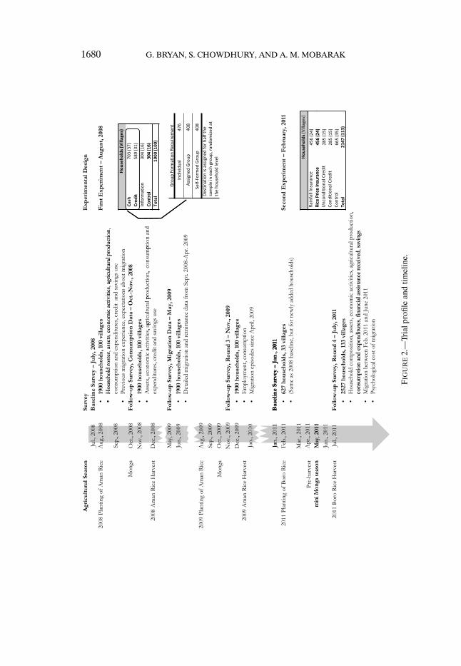
signed additional conditionalities to subsets of households within the village.A trial profile in Figure 2 provides details. Some households were required tomigrate in groups, and some were required to migrate to a specific destination.These conditionalities created random within-village variation, which we useas instrumental variables to study spillover effects from one person to another.
3.1. Data
We conducted a baseline survey of the 1900 sample households in July 2008,just before the onset of the 2008 monga. We collected follow-up data in De-cember 2008, at the end of the 2008 monga season. These two rounds involveddetailed consumption modules in addition to data on income, assets, credit,and savings. The follow-up also asked detailed questions about migration expe-riences over the previous four months. We learned that many migrants had notreturned by December 2008, and therefore conducted a short follow-up surveyin May 2009 to get more complete information about households’ migrationexperiences. To study the longer-run effects of migration, and re-migration be-havior during the next monga season, we conducted another follow-up surveyin December 2009. This survey only included the consumption module and amigration module. We conducted a new round of experiments to test our the-ories in 2011, and therefore collected an additional round of follow-up dataon the re-migration behavior of this sample in July 2011. In summary, detailedconsumption data were collected over three rounds: in July 2008 (baseline),December 2008, and December 2009. Migration behavior data were collectedin December 2008, May 2009, December 2009, and July 2011, which jointlycover three seasons in 2008, 2009, and 2011.
Table I shows that there was pretreatment balance across the randomly as-signed groups in terms of the variables that we will use as outcomes in theanalysis to follow. A Bonferroni multiple comparison correction for 27 inde-pendent tests requires a significance threshold of α = 0�0019 for each test torecover an overall significance level of α= 0�05. Using this criterion, no differ-ences at baseline are statistically meaningful.
4. PROGRAM TAKE-UP AND THE EFFECTS OF SEASONAL MIGRATION
In this section, we describe the main results of our initial (2008) experiment.Section 4.1 provides results on migration behavior. We first document the im-pact of the incentive on migration during the 2008 monga season (the seasonfor which the incentive was in place). We then document the ongoing impact ofthe incentive on migration in 2009 and 2011 (one and three years, respectively,after the incentive was removed). In Section 4.2, we look at the effect of thetreatment on consumption at the origin (both in the short run: 2008, and thelong run: 2009). We first provide both intent-to-treat (ITT) and local averagetreatment effect (LATE) estimates for consumption in December 2008, and
1680 G. BRYAN, S. CHOWDHURY, AND A. M. MOBARAK
FIG
UR
E2.
—Tr
ialp
rofil
ean
dtim
elin
e.

UNDERINVESTMENT IN A PROFITABLE TECHNOLOGY 1681
TABLE I
RANDOMIZATION BALANCE ON OBSERVABLES AT BASELINEa
Incentivized Non-Incentivized
Cash Credit Control Info Diff. (I − NI) p-Value
Consumption of food 805.86 813.65 818.68 768.64 15.84 0.638(19.16) (40.91) (31.76) (18.00) (33.57)
Consumption of non-food 248.98 262.38 248.4 237.35 12.23 0.278(5.84) (6.74) (9.28) (7.99) (11.20)
Total consumption 1054.83 1076.03 1067.08 1005.99 28.06 0.465(21.11) (42.08) (34.55) (22.77) (38.29)
Total calories 2081.19 2079.51 2099.3 2021.31 20.25 0.585(per person per day) (20.34) (22.76) (30.44) (32.56) (36.99)
Calories from protein 45.66 45.3 46.26 44.75 −0.01 0.992(per person per day) (0.54) (0.57) (0.77) (0.85) (0.92)
Consumption of meat products 25.04 18.24 27.13 20.71 −1.97 0.594(2.58) (2.0) (3.24) (2.90) (3.69)
Consumption of milk and eggs 11.74 9.77 9.96 10.77 0.48 0.675(0.79) (0.80) (1.12) (1.19) (1.13)
Consumption of fish 42.17 39.86 41.36 45.98 −2.56 0.496(1.83) (1.79) (2.76) (2.89) (3.74)
Consumption of children’s education 24.14 27.14 22.31 16.95 6.01 0.016∗∗
(1.75) (2.31) (2.34) (2.1) (2.44)
Consumption of clothing and shoes 37.31 38.8 39.24 38.35 −0.80 0.693(0.79) (0.90) (1.41) (1.30) (2.02)
Consumption of health for male 52.39 52.9 63.72 47.45 −2.86 0.696(5.14) (5.23) (8.15) (6.48) (7.28)
Consumption of health for female 37.34 52.5 39.36 49.75 −0.31 0.961(3.52) (5.75) (5.68) (7.51) (6.26)
Total saving in cash 1345.55 1366.37 1418.29 1611.05 −160.56 0.255(conditional on positive savings) (97.54) (121.26) (135.04) (185.56) (140.09)
HH size 3.93 3.98 3.99 4.05 −0.07 0.473(0.05) (0.05) (0.08) (0.08) (0.10)
HH head education 0.25 0.24 0.25 0.22 0.01 0.6281 = Educated (0.02) (0.02) (0.02) (0.02) (0.03)
Number of males 1.19 1.22 1.18 1.18 0.03 0.515Age > 14 (0.02) (0.02) (0.03) (0.03) (0.04)
Number of children 1.01 1.05 1.08 1.15 −0.09 0.093Age < 9 (0.03) (0.04) (0.05) (0.05) (0.05)
Household has pucca walls 0.29 0.32 0.27 0.30 0.02 0.55(0.02) (0.02) (0.03) (0.03) (0.04)
Literacy score average 3.37 3.40 3.48 3.30 −0.01 0.84(0.04) (0.04) (0.05) (0.06) (0.06)
(Continues)

1682 G. BRYAN, S. CHOWDHURY, AND A. M. MOBARAK
TABLE I—Continued
Incentivized Non-Incentivized
Cash Credit Control Info Diff. (I − NI) p-Value
Subjective expectation: 78.79 78.62 78.38 75.72 1.66 0.47Monga occurrence this year (0.77) (0.88) (1.15) (1.35) (2.32)
Subjective expectation: 58.53 60.82 58.38 57.40 1.68 0.41Will get social network help in Dhaka (1.07) (1.21) (1.64) (1.61) (2.04)
Subjective expectation: 52.53 52.90 52.42 51.15 0.91 0.70Can send remittance from Dhaka (1.13) (1.25) (1.78) (1.72) (2.40)
Ratio of food expenditure over 0.77 0.75 0.77 0.77 −0.01 0.21total consumption in round 1 (0.003) (0.09) (0.01) (0.004) (0.01)
Average skill score received by network 6.53 6.49 6.24 6.20 0.27 0.24(0.05) (0.27) (0.07) (0.07) (0.23)
Applied and refused for credit 0.03 0.04 0.04 0.04 −0.00 0.75or did not apply because of (0.01) (0.004) (0.01) (0.01) (0.01)insufficient collateral
Received credit from NGO, family 0.68 0.65 0.70 0.60 0.02 0.55and friends, or money lender (0.02) (0.02) (0.03) (0.03) (0.04)
Migration to Bogra in round 1 0.11 0.10 0.16 0.12 0.03 0.30(0.01) (0.01) (0.02) (0.02) (0.03)
aFirst four columns show the mean of the corresponding variables; fifth column shows the difference betweenthe means of incentivized and non-incentivized groups. Standard errors are reported in parentheses. Differences andp-values are derived from linear regression the variable of interest as the dependent variable, a binary variable equalto 1 if treatment group and 0 else as the independent variable; robust standard errors clustered at the village levelare reported. All expenditure categories are monthly totals, reported on per capita basis based on the size of thehousehold. ∗∗∗p< 0�01, ∗∗p< 0�05, ∗p< 0�1.
then also look at the ongoing impact of the incentives on consumption in 2009.In Section 4.3, we look at migration income and savings at the destination.
4.1. Migration and Re-Migration
Table II reports the take-up of the program across the four groups labeledcash, credit, information, and control. We have 2008 migration data from twofollow-up surveys, one conducted immediately after the monga ended (in De-cember 2008), and another in May 2009. The second follow-up was helpful forcross-checking the first migration report,12 and for capturing the migration ex-periences of those who left and/or returned later. The two sets of reports were
12Since an incentive was involved, we verified migration reports closely using the substantialfield presence of our partner NGOs, by cross-checking migration dates in the two surveys con-ducted six months apart, by cross-checking responses across households who reported migratingtogether in a group, and finally, by independently asking neighbors. The analysis (available onrequest) shows a high degree of accuracy in the cross reports and, importantly, that the accuracyof the cross reporting was not different in incentivized villages.

UNDERINVESTMENT IN A PROFITABLE TECHNOLOGY 1683
TABLE II
PROGRAM TAKE-UP RATESa
Incentivized Cash Credit Not Incentivized Info Control Diff. (I − NI)
Migration rate in 2008 58.0% 59.0% 56.8% 36.0% 35.9% 36.0% 22.0∗∗∗
(1.4) (1.9) (2.1) (2.0) (2.8) (2.8) (2.4)
Migration rate in 2009 46.7% 44.6% 49.1% 37.5% 34.4% 40.5% 9.2∗∗∗
(1.4) (1.9) (2.1) (2.0) (2.8) (2.9) (2.5)
Migration rate in 2011b 39% 32% 7.0∗∗
(2.1) (2.5) (3.3)
aStandard errors in parentheses. ∗∗∗p < 0�01, ∗∗p < 0�05, ∗p < 0�1. Diff. Incentivized − Not Incentivized teststhe difference between migration rates of incentivized and non-incentivized households, regardless of whether theyaccepted our cash or credit. No incentives were offered in 2009.
bFor re-migration rate in 2011, we compare migration rates in control villages that never received any incentivesto the subset of 2008 treatment villages that did not receive any further incentives in 2011. Note that migration wasmeasured over a longer period (covering the main monga season) in 2008 and 2009, and a different time period (themini-monga season) in 2011.
quite consistent with each other, and the first row of Table II shows the morecomplete 2008 migration rates obtained in May 2009.
In Table II, we define a household as having a seasonal migrant if at leastone household member migrated away in search of work between September2008 and April 2009. This extended definition of the migration window ac-counts for the possibility that our incentive merely moved forward migrationthat would have taken place anyway. This window captures all migration duringthe Aman cropping season and, as a consequence, all the migration associatedwith monga.
About a third (36.0%) of households in control villages sent a seasonal mi-grant.13 Providing information about wages and job opportunities at the desti-nation had no effect on the migration rate (the point estimate of the differenceis 0.0% and is tightly estimated). Either households already had this informa-tion, or the information we made available was not useful or credible. Withthe $8.50 (+ $3) cash or credit treatments, the seasonal migration rate jumpsto 59.0% and 56.8%, respectively. In other words, incentives induced about22% of the sample households to send a migrant. The migration response tothe cash and credit incentives is statistically significant relative to control orinformation, but there is no statistical difference between providing cash andproviding credit—a fact that our model will later account for. Since house-holds appear to react very similarly to either incentive, we combine the impact
13In a large survey of 482,000 households in the Rangpur region, 36.0% of people report us-ing “out-migration” as a coping mechanism for the monga (Khandker, Khaleque, and Samad(2011)). Our result appears very consistent with the large-sample finding. Interestingly, surveyrespondents who qualified for government safety-net benefits were no more likely to migratethan households that did not.

1684 G. BRYAN, S. CHOWDHURY, AND A. M. MOBARAK
of these two treatments for expositional simplicity (and call it “incentive”) formuch of our analysis, and compare it against the combined information andcontrol groups (labeled “non-incentive”).
The second and third rows of Table II compare re-migration rates in sub-sequent years across the incentive and non-incentive groups. We conductedfollow-up surveys in December 2009 and in July 2011 and asked about migra-tion behavior in the preceding lean seasons, but we did not repeat any of thetreatments in the villages used for the comparisons in 2008. Strikingly, the mi-gration rate in 2009 was 9 percentage points higher in treatment villages, andthis is after the incentives were removed. Section 6.3.1 will show that this isalmost entirely due to re-migration amongst a subset who were induced to mi-grate in 2008. In other words, migration appears to be an “experience good.”The July 2011 survey measured migration during the other (lesser) lean seasonthat coincides with the pre-harvest period for the second (lesser) rice harvest.Even two and a half years later, without any further incentive, the migrationrate remains 7 percentage points higher in the villages randomly assigned tothe cash or credit treatment in 2008.14
We learn two important things from this re-migration behavior. First, thepropensity to re-migrate absent further inducements serves as a revealed pref-erence indication that the net benefits from migration were positive for many,and/or that migrants developed some asset during the initial experience thatmakes future migration a positive expected return activity.15 Second, the per-sistence of re-migration from 2009 to 2011 (with four potential migration sea-sons in between) suggests that households learned something valuable or grewsome real asset from the initial migration experience. This persistence makes itunlikely that some households simply got lucky one year, and then it took themseveral tries to determine (again) that they are actually better off not migrat-ing. It also reduces the likelihood that our results are driven by a particularlygood migration year in 2008.
This strong repeat migration also suggests that migration is an absorbingstate, at least for some portion of the population. As we discuss further inSections 6 and 8, this makes it hard to understand how our initial incentive wassuccessful in inducing so much migration.
4.2. Effects of Migration on Consumption at the Origin
We now study the effects of migration on consumption expendituresamongst remaining household members during the monga season. Consump-
14Overall in our sample, 953 out of 1871 sample households sent a migrant in 2008 (and 723 ofthem traveled before our December 2008 follow-up survey), and 800 households sent a seasonalmigrant during the 2009 monga season.
15All socio-economic outcomes we measure using our surveys will necessarily be incomplete,since it is not possible to combine the social, psychological, and economic effects of migration inone comprehensive welfare measure. The revealed re-migration preference is therefore a usefulcomplement to other economic outcomes that we use in the analysis below.

UNDERINVESTMENT IN A PROFITABLE TECHNOLOGY 1685
tion is a broad and useful measure of the benefits of migration, aggregatingas it does the impact of migrating on the whole family (Deaton (1997)), andtakes into account the monetary costs of investing (although it neglects non-pecuniary costs). Consumption can be comparably measured for migrant andnon-migrant families alike, and it overcomes the problems associated withmeasuring the full costs and benefits of technology adoption highlighted inFoster and Rosenzweig (2010). Our consumption data are detailed and com-prehensive: we collect expenditures on 318 different food (255) and non-food(63) items (mostly over a week recall, and some less-frequently-purchaseditems over bi-weekly or monthly recall), and aggregate up to create measuresof food and non-food consumption and caloric intake.
We first present pure experimental (intent-to-treat) estimates in Table IIIwith consumption measures regressed on the randomly assigned treatments:cash, credit, and information for migration. Our regressions take the form
Yivj = α+β1Cashivj +β2Creditivj +β3Informationivj +ϕj + υivj�
where Yivj is per capita consumption (money spent on food, non-food, totalcalories, protein, meat, education, etc. in turn) for household i in village v insubdistrict j in 2008, and ϕj are fixed effects for subdistricts. Standard errorsare clustered by village, which was the unit of randomization (and this will betrue for all our analysis). The first three columns in Table III show β1, β2, andβ3—the coefficients on cash, credit, and information—and each row repre-sents a different regression on a different dependent variable. Panel A studiesthe effects on 2008 consumption, while Panel B examines consumption mea-sured in December 2009, after the next monga season. The dependent vari-ables are household averages using the set of people reported to be living inthe household for at least 7 days at the time of the survey as the denominator.We discuss the appropriate choice of denominator in more detail below.
Panel A shows that both the cash and credit treatments—which induced 21–24% more migration—result in statistically significant increases in food andnon-food consumption in 2008. Total consumption increased by about 97 Takaper household member per month in the ‘cash’ villages, which represents abouta 10% increase over consumption in the control group. The increase in creditvillages was 8%. The information treatment, which did not induce any addi-tional migration, does not result in any significant increases in consumption.Calories per person per day increase by 106 under the ‘cash’ treatment.
Since both cash and credit treatments led to greater migration (Table II), col-umn 4 reports the intent-to-treat estimates for these two incentive treatmentsjointly. Average monthly household consumption increases by 68 Taka in theseincentive villages (7% over control group), and this results in 142 extra caloriesper person per day. Column 5 indicates that these effects are generally robustto adding some controls for baseline characteristics.

1686G
.BR
YA
N,S.C
HO
WD
HU
RY
,AN
DA
.M.M
OB
AR
AK
TABLE III
EFFECTS OF MIGRATION BEFORE DECEMBER 2008 ON CONSUMPTION AMONGST REMAINING HOUSEHOLD MEMBERSa
ITT
Cash Credit Info ITT ITT IV IV OLS Mean
Panel A: 2008 ConsumptionConsumption of food 61�876∗∗ 50�044∗ 15.644 48�642∗∗ 44�183∗ 280�792∗∗ 260�139∗∗ 102�714∗∗∗ 726�80
(29.048) (28.099) (40.177) (24.139) (23.926) (131.954) (128.053) (17.147)
Consumption of non-food 34�885∗∗∗ 27�817∗∗ 22.843 20�367∗∗ 16�726∗ 115�003∗∗ 99�924∗ 59�085∗∗∗ 274�46(13.111) (12.425) (17.551) (9.662) (9.098) (56.692) (51.688) (8.960)
Total consumption 96�566∗∗∗ 76�743∗∗ 38.521 68�359∗∗ 60�139∗∗ 391�193∗∗ 355�115∗∗ 160�696∗∗∗ 1000�87(34.610) (33.646) (50.975) (30.593) (29.683) (169.431) (158.835) (22.061)
Total calories 106�819∗ 93.429 −85.977 142�629∗∗∗ 129�901∗∗∗ 842�673∗∗∗ 757�602∗∗∗ 317�495∗∗∗ 2090�26(per person per day) (62.974) (59.597) (76.337) (47.196) (48.057) (248.510) (250.317) (41.110)
(Continues)

UN
DE
RIN
VE
STM
EN
TIN
APR
OF
ITAB
LE
TE
CH
NO
LO
GY
1687
TABLE III—Continued
ITT
Cash Credit Info ITT ITT IV IV OLS Mean
Panel B: 2009 ConsumptionConsumption of food 34.273 22.645 −30.736 43�983∗∗ 34�042∗ 230�811∗∗ 186�279∗ 1.687 872�69
(23.076) (23.013) (29.087) (17.589) (18.110) (100.536) (96.993) (14.687)
Consumption of non-food 3.792 31�328∗ −8.644 21�009∗ 14.877 110�324∗ 74.216 6.133 323�31(16.186) (18.135) (20.024) (11.954) (12.031) (65.333) (63.792) (10.312)
Total consumption 38.065 53.973 −39.380 64�992∗∗∗ 48�919∗ 341�135∗∗ 260�495∗∗ 7.820 1196�01(30.728) (34.057) (39.781) (23.958) (24.713) (137.029) (131.851) (21.044)
Total calories 83.242 23.995 −81.487 95�621∗∗ 78�564∗ 510�327∗∗ 434�602∗∗ 20.361 2001�27(per person per day) (52.766) (62.207) (60.141) (39.187) (40.600) (221.010) (216.670) (28.392)
Controls? No No No No Yes No Yes NoaRobust standard errors in parentheses, clustered by village. ∗∗∗p< 0�01, ∗∗p< 0�05, ∗p< 0�1. Each row is a different dependent variable (in column 1). In the IV columns,
these dependent variables are regressed on “Migration,” which is a binary variable equal to 1 if at least one member of the household migrated and 0 otherwise. The last columnreports sample mean of the dependent variable in the control group. All consumption (expenditure) variables are measured in units of Takas per person per month, except CaloricIntake which is measured in terms of calories per person per day. Some expenditure items in the survey were asked over a weekly recall and other less frequently purchased itemswere asked over a bi-weekly or monthly recall. The denominator of the dependent variable (household size) is the number of individuals who have been present in the housefor at least seven days. Additional controls included in columns 5 and 7 were: household education, proxy for income (wall material), percentage of total expenditure on food,number of adult males, number of children, lacked access to credit, borrowing, total household expenditures per capita measured at baseline, and subjective expectations aboutmonga and social network support measured at baseline.

1688 G. BRYAN, S. CHOWDHURY, AND A. M. MOBARAK
Next, we show the local average treatment effect (LATE), the consumptioneffect of migration for those households that were induced to migrate by ourintervention. This is a well-defined and policy-relevant parameter in our set-ting: programs providing credit for migration and even incentivizing migrationseem to be of direct policy interest, and we think it unlikely that any householdswere dissuaded from migrating by our incentive.16 We calculate this effect byestimating
Yivj = α+βMigrantivj + θXivj +ϕj + υivj�
where Migrantivj is a binary variable equal to 1 if at least one member of house-hold migrated during monga in 2008 and 0 otherwise, and Xivj is a vector ofhousehold characteristics at baseline that we sometime control for. The en-dogenous choice to migrate is instrumented with whether or not a householdwas randomly placed in the incentive group:
Migrantivj = λ+ ρZv + γXivj +ϕj + εivj�
where the set of instruments Zv includes indicators for the random assignmentat the village level into one of the treatment (cash or credit) or control groups.First-stage results in Appendix Table A.I verify that the random assignmentsto cash or credit treatments are powerful predictors of the decision to migrate.
The intervention may have changed not only households’ propensity to mi-grate on the extensive margin, but also who within the household migrates,how long they travel, the number of migration episodes on the intensive mar-gin. Such changes may affect the interpretation of the IV estimates. AppendixTable A.II shows that the treatment does not significantly alter whether thehousehold sends a male or female migrant, or the number of trips per migrant,or the number of migrants or trips per household (on the intensive margin,conditional on someone in the household migrating once). The effects are con-centrated on the extensive margin, inducing migration among households whowere previously not migrating at all.17 However, the treatment does make itmore likely that older, heads of households become more likely to migrate.
16Since the incentive arm included the information script, it may in theory have altered thebehavior of households that did not migrate, which would threaten the exclusion restriction. Wehave verified that the information-only treatment had no effect (relative to control) on savings in2008 or migration in 2009, or a broader range of outcomes. It is therefore unlikely that the infor-mation component of the incentive treatment had independent effects that violate the exclusionrestriction. Furthermore, all incentive treatment effects we report in this section are robust toomitting the information-only group entirely, and comparing only to the pure control arm.
17The migrant is almost always male (97%), and often the household head (84% in treatmentvillages and 76% in control), who is often the only migrant from that household (93%). Migrantsmake 1.73 trips on average during the season, which implies that migrants often travel multipletimes within the season. The first trip lasts 42 (56) days for treatment (control) group migrants.They return home with remittance and to rest, and travel again for 40 (40) days or less on anysubsequent trips.

UNDERINVESTMENT IN A PROFITABLE TECHNOLOGY 1689
IV estimates using treatment assignment are always larger than OLS esti-mates. This likely reflects the fact that rich households at the upper end of oursample income distribution are not very likely to migrate (baseline income hasa negative coefficient in the first-stage regression in Appendix Table A.I). Inthe IV specification, per capita food, non-food expenditures, and caloric in-take among induced migrant households increase by 30% to 35% relative tonon-migrant households. This is very similar to the 36% consumption gainsfrom migration estimated by Beegle, De Weerdt, and Dercon (2011) for Tan-zania. Finally, none of the results discussed above are sensitive to changes inbaseline control variables.
In terms of magnitude of effects, monthly consumption among migrant fam-ilies increases by about $5 per person, or $20 per household, due to inducedmigration. Our survey only asked about expenditures during the second monthof monga, and the modal migrant in our sample had not yet returned home(which includes cases where they may have returned once, but left again). Wetherefore expect the effects to persist for at least another month, and the to-tal expenditure increase therefore easily exceeds the amount of the treatment($8.50). Furthermore, if households engage in consumption smoothing, thensome benefits may persist even further in the future. In any case, the $8.50 isspent on transportation costs two months prior to the consumption survey.
It is not straightforward to evaluate the returns to migration based on theseestimates, and the precise value will depend on assumptions about the periodover which the consumption gains are realized, and how to treat the cost thatsome migrants choose to incur to return home and take a second trip. Un-der a reasonable assumption that the consumption gains are realized overthe 2 months of the monga period, households consume an extra Tk. 2840(Tk. 355 per capita per month estimated in Table III ∗ 4 household mem-bers ∗ 2 months) during the monga by incurring a migration cost of Tk. 1038(Tk. 600/trip ∗ 1.73 trips). This implies a gross return of 273%, ignoring anydisutility from separation.
Since the act of migration both increases the independent variable of interestand possibly reduces the denominator of the dependent variable (householdsize at the time of interview), any measurement error in the date that migrantsreport returning can bias the coefficient on migration upwards. We addressthis problem directly by studying the effects of migration in 2008 on consump-tion in 2009 (where household size is computed using a totally different surveyconducted over a year later). Panel B of Table III shows that 2009 effects areabout 60–75% as large as the consumption effects in 2008 across both ITT andLATE specifications, but still statistically significant. Migration is associatedwith a 28% increase in total household consumption. The LATE specificationfor 2009 is more difficult to interpret: many of those induced to migrate in 2008were induced to re-migrate a year later, but they could have also re-invested

1690 G. BRYAN, S. CHOWDHURY, AND A. M. MOBARAK
their 2008 earnings in other ways that lead to long-run consumption gains.18
Appendix Table A.IV examines effects on a few detailed categories of con-sumption. We focus on protein consumption, because this is a marker of wel-fare in very poor populations. We see that migration leads to some statisticallyand quantitatively significant increase in the consumption of protein, especiallyfrom meat and fish (but not milk and eggs). For the Bangladesh context, thisreflects a shift toward a higher quality diet, as meat and fish are consideredmore attractive, “tasty” sources of protein. Educational expenditures on chil-dren also increase significantly, but there is no significant change in medicalexpenditures for males or females. There are no changes in female labor forceparticipation, school attendance, or agricultural investment.
4.3. Income and Savings at the Destination
Next, we examine the data on migrants’ earnings and savings at the desti-nation to see whether the magnitude of consumption gains we observe at theorigin are in line with the amount migrants earn, save, and remit. Informationon earnings and savings at the destination were only collected from migrants,and these are not experimental estimates; they merely help to calibrate theconsumption results. Table IV shows that migrants in the treatment group earnabout $105 (7451 Taka) on average and save about half of that. The averagesavings plus remittance is about a dollar a day. Remitting money is difficult andmigrants carry money back in person, which is partly why we observe multiplemigration episodes during the same lean season. Therefore, joint savings plusremittances is the best available indicator of money that becomes availablefor consumption at the origin. The destination data suggest that this amountis about $66 (4600 Taka) for the season. The “regular” migrants in the controlgroup earn more per episode, save, and remit more per day relative to migrantsin the treatment group. This is understandable, since the migrants we induceare new and relatively inexperienced in this activity.
We can compute experimental (ITT) estimates on total income (and sav-ings), by aggregating across all income sources at the origin and the destina-tion. Income is notoriously difficult to measure in these settings, with incomerealized from various sources—agricultural wages, crop income, livestock in-come, enterprise profits—parts of which are derived from self-employmentor family employment where a financial transaction may not have occurred.Appendix Table A.V shows ITT and IV estimates. Households in the treat-ment group have 585 extra Taka in earnings, and hold 592 extra Taka in sav-ings. In the IV specification, migration is associated with 3300 extra Taka in
18Since the migration decision is serially correlated, measurement error in 2009 migrationdates can also bias our estimates. Appendix Table A.III shows the results of a number of othersensitivity checks on the consumption results by varying the definition of household size (thedenominator). The results are robust.

UNDERINVESTMENT IN A PROFITABLE TECHNOLOGY 1691
TABLE IV
MIGRANT EARNINGS AND SAVINGS AT DESTINATION(DATA FOR MIGRANTS ONLY; NON-EXPERIMENTAL)a
All Migrants Incentivized Not Incentivized Diff. Observations
Total savings by household 3490.47 3506.59 3434.94 71.65 951(97.22) (110.83) (202.80) (232.91)
Total earnings by household 7777.19 7451.27 8894.40 −1443�129∗∗ 952(244.77) (264.99) (586.14) (583.83)
Savings per day 56.76 56.46 57.79 −1.33 905(1.15) (1.29) (2.56) (2.77)
Earnings per day 99.39 96.09 111.15 −15�06∗∗ 926(1.75) (1.92) (4.0) (4.2)
Remittances per day 18.34 16.94 23.33 −6�39∗∗ 927(1.06) (1.19) (2.28) (2.55)
One-way travel cost per episode 264.55 264.12 266.00 −1.88 953(3.41) (3.80) (7.62) (8.16)
aStandard errors are reported in parentheses. ∗∗∗p< 0�01, ∗∗p< 0�05, ∗p< 0�1. The “Diff.” columns tests statisti-cal differences between incentivized and non-incentivized groups, with robust standard errors clustered at the villagelevel reported in parentheses. The measures for total savings and earnings, and savings and earnings per day do not in-clude outliers (less than 20,000 for total savings and 120,000 for earnings, individuals savings per day less than 500 andindividuals earnings per day less than 700). Travel cost refers to the cost of food and travel to get to the destination.Average migration duration 76 days.
earnings and savings. We also examine effects on an anthropometric measurewe collected—each child’s middle-upper-arm-circumference (MUAC). The IVspecifications suggest that migrants’ children’s MUAC grew an extra 5–11 mm,but the result is not statistically significant. MUAC was measured in December2008, soon after the initial inducement to migrate.
Appendix Table A.VI provides further descriptive statistics on the number ofmigration episodes and average earnings by sector and by destination. Dhaka(the largest urban area) is the most popular migration destination, and a largefraction of migrants to Dhaka work in the transport sector (i.e., rickshaw-pulling). Many others work for a daily wage, often as unskilled labor at con-struction sites. At or around other smaller towns that are nearer to Rangpur,many migrants work in agriculture, especially in potato-growing areas that fol-low a different seasonal crop cycle than in rice-growing Rangpur. Migrantsearn the most in Dhaka and at other “non-agricultural destinations”: about5100 Taka or $71 per migration episode, which translates to $121 per house-hold on average, given multiple trips. Those working for daily wages in thenon-agricultural sector (e.g., construction sites, brick kilns) earn the most.
It is difficult to infer the income these migrants would have received had theynot migrated. Observed average migrant earnings at the destination (100 Takaper day) do compare favorably to the earnings of the sub-sample of non-migrants with salaried employment at the origin (65 Taka per day) and to the

1692 G. BRYAN, S. CHOWDHURY, AND A. M. MOBARAK
profits of entrepreneurs at the origin (61 Taka per day). There is heterogeneityaround that average, which introduces some risk, and we will discuss this inSection 6.
5. THEORY
We have documented three facts: (1) A large number of households weremotivated to migrate in response to the 600 Taka incentive. (2) There werepositive returns to the induced migration on average, indicating that house-holds were not migrating despite a positive expected profit. (3) A large portionof the households that were incentivized to migrate continued to send a sea-sonal migrant in subsequent years.
These three facts taken together suggest that the people of Rangpur, andperhaps others in the developing world, are failing to capitalize on an ex-tremely profitable opportunity, and suggest a potential role for policy in fa-cilitating migration. Two issues, however, need to be addressed: first, becausethese results are unlikely to generalize to all settings, it is important to under-stand the circumstances in which we expect to see migration outcomes similarto the ones documented above; and second, it is important to understand theoptimal policy response to our findings. To address these issues, this sectionprovides a simple model that can help to rationalize the findings. The modelcan be used to characterize settings in which our experimental results are likelyto replicate and can be used to think about optimal policy.
The model we provide emphasizes three key elements: risk, subsistence,and learning about the profitability of migration. These elements help to ex-plain why a household would not migrate despite positive returns, and also thestrong re-migration rates. Further, our model also incorporates the empiricallyrealistic assumptions that households face credit constraints and can save, bothfor migration and to buffer against income shocks.
To assess the empirical fit of the model, we undertake two exercises. First, weuse the model to frame a deeper discussion of the data in Section 6 and arguethat several patterns in the data are qualitatively consistent with our simpleframework. Second, in Section 7, we ask whether the model can make sense ofthe data, quantitatively. To do this, we calibrate the model and then ask howrisk averse a potential migrant would have to be for our model to generate ourexperimental results. Here we find that the model is not able to quantitativelyreplicate our experimental findings for reasonable parameter values. We arguethat there are two main reasons for this failure: first, forward-looking migrantsshould foresee the strong positive re-migration rate and hence the long-termrisk reduction advantages of migration; second, given the profitability of mi-gration, households should be saving up in order to experiment.
We interpret the results of this section as follows. First, our qualitative anal-ysis strongly suggests that risk, subsistence, and the need to experience migra-tion are important elements in explaining our experimental results. We predict

UNDERINVESTMENT IN A PROFITABLE TECHNOLOGY 1693
these three elements will be present in other settings where migration is prof-itable but underutilized. Second, our quantitative results suggest that the be-havior we document (low migration rates but high returns) remains somewhatof a puzzle: there is some element that we do not understand. In Section 8, weprovide some discussion of what this element may be, but because we lack thedata to come to a definitive conclusion, we leave the resolution of the puzzleto future work. Such work could help us to get a stronger understanding of thetwo questions that motivate this section: where do we expect to see positive un-realized returns, and what exactly should policymakers do in response to thesereturns?
5.1. Baseline Model
We consider the migration and consumption choices of an infinitely livedhousehold in discrete time. In each time period, a state of the world s ∈ S isdrawn according to the distribution μ and the household receives income ys.19
We refer to this as background income and assume the process is independentand identically distributed (i.i.d.).20 A household that enters the period withassets A and receives background income y has cash on hand x = A + y . Weassume that the household can save at a gross interest rate R, but cannot bor-row for consumption purposes.21 Therefore, consumption is less than cash onhand (c ≤ x) in any period.
The household faces uncertainty. With probability πG the household is typeG—good at migrating—and receives a positive (net) return to migrating of m.With probability (1 −πG) the household is type B—bad at migrating—and re-ceives no return to migrating, but faces a cost F if it does choose to migrate.There are two possible interpretations of πG. The first is that each migratorhas a set characteristic, which determines whether he or she is good at migrat-ing, and is revealed at the destination. The second is that πG is the probability
19We assume that all households face the same distribution of background income. This is astrong simplifying assumption. In practice, there are likely to be poorer and wealthier households.Our model suggests that those that are very poor will not migrate because it is too risky. Inpractice, those that are very rich will likely not migrate because they do not need to supplementincome, and those that are in the middle migrate because they can afford to and benefit fromdoing so. This is consistent with a slightly altered version of the model presented here in whichmigration truncates the distribution of earning from below. We have explored this alternativemodel, but find that it leads to similar quantitative results. We do not pursue this approach inthe main text, as the model is more complicated; because cash on hand is not a sufficient statevariable, it is also more computationally expensive to use for simulations.
20See Deaton (1991) for a discussion of the impact of relaxing this assumption. We think it is areasonable assumption in our setting and maintain it throughout.
21Households have access to microfinance from a range of sources, but the conditions asso-ciated with such loans (only for female borrowers, to be used for entrepreneurial ventures, re-quiring bi-weekly repayment) imply that households are still credit constrained for consumptionsmoothing or migration.

1694 G. BRYAN, S. CHOWDHURY, AND A. M. MOBARAK
of finding a connection at the destination within a reasonable search time.22
In either case, we think of type (once it is revealed) as being a household-specific parameter, and not something that can be easily learned or transferredover from other households in the village. We further assume that this uncer-tainty resolves after one period of experimentation with migration. Migrationis, therefore, to be thought of as an experience good. This assumption is moti-vated by reports that migrants need to find a potential employer at the destina-tion and convince that employer to trust them. Once this link is established itis permanent, but some migrants will not be able to form such a link. A leadingexample from our data is convincing the owner of a rickshaw that you can betrusted with his valuable asset.23
A household that knows it is bad at migrating will never migrate and is essen-tially a Deaton (1991) buffer stock saver. With cash on hand x, such a house-hold solves
B(x)= maxc≤x
[u(c)+ δ
∫S
B(yS +R(x− c)
)dμ(s)
]�
where u is a standard strictly increasing, strictly concave utility function and δ isthe household’s discount factor. A household that knows it is good at migratingwill always migrate and solves a similar problem, but with a higher income.With cash on hand x, a household that is a good migrator has value
G(x) = maxc≤x+m
[u(c)+ δ
∫S
G(yS +R(x+m− c)
)dμ(s)
]�
With this formulation, we are assuming that the household can migrate beforeit makes its consumption decision; this means that a household that knows it isa good migrator can always migrate regardless of credit constraints.
We are interested in the behavior of a household that has never migratedbefore. In each period, such a household chooses both whether to migrate and
22The two alternatives differ in one key aspect: what are the choices open to a household thathas migrated in the past and found itself to be a bad migrator? The first alternative implies theywill never migrate again, because they know they are bad at migrating, but the second impliesthat they may migrate again and take another draw to see if they can find a connection. We writethe model in this section with the first possibility in mind because it is simpler. However, when wedo our calibration we assume that a household that is found to be bad can continue to migrateand have another draw, in line with the second interpretation. This errs on the side of lettingthe model fit the data, because more households will be affected by the incentive. We also favorthe second interpretation when we consider the interpretation of our insurance experiments inSection 6.2.1.
23We thank an anonymous referee for clarification on this point and also the term experiencegood. Direct experience with migration may also be required if it is difficult to receive crediblereports on employment conditions at the destination. McKenzie, Gibson, and Stillman (2007)provided some evidence that migrators report incorrect information.

UNDERINVESTMENT IN A PROFITABLE TECHNOLOGY 1695
consumption/savings. If it migrates, it discovers that it is a good migrator withprobability πG and has value G(x). If, however, the household migrates anddiscovers that it is a bad migrator, then it has paid a cost F and receives valueB(x−F). We think of the cost F as being the cost of transport and lost incomewhile the migrator searches for work. The household will choose to migrate ifthe expected utility of migration is greater than that of not migrating. There-fore, a household that has never migrated before, and has cash on hand x,solves
V (x) = max{
maxc≤x
[u(c)+ δ
∫S
V(ys +R(x− c)
)dμ(s)
]�
πGG(x)+ (1 −πG)B(x− F)
}�
Migration is risky in this model. A household that turns out to be a bad mi-grator pays a cost F but receives no benefit. This has two implications. First,the household is credit constrained and will have to forego consumption in thecurrent period. Second, the household may face a bad shock in the next period,but will have no buffer stock saving to smooth consumption. Hence, the modelhas a role for background risk which, given the assumptions we make aboutthe utility function, implies that the riskier the background income process is,the less likely is migration for any particular level of cash on hand.24
Throughout our discussion, we assume that the household faces a sub-sistence constraint. We model this by assuming that u(c) = u(c − s) withlimx→0 u
′(x) = ∞, limx→0 u(x) = −∞, and limx→0u′′(x)u′(x) = ∞. That is, there is
a level of consumption s at which the household is unwilling to consider de-creasing consumption for any reason, and the household becomes infinitelyrisk averse. We think of s as a point at which survival requires the householdto spend all its current resources on food, with the implication that householdmembers face a threat of serious illness or death if they do not consume atleast s. The possibility that consumption is close to this point in our data ishighlighted by the fact that the monga famine regularly claims lives. We alsoshow below that many households’ expenditure seems to fall below what wouldbe required for a minimal subsistence diet. We believe it reasonable to assumethat a household that has such a low consumption level would not be willing totake on any risk. For our simulations, we use a fairly standard utility functionthat incorporates a subsistence point: u(c) = (c−s)1−σ
1−σ.
The model is related to Deaton’s buffer stock model, several models fromthe poverty trap literature (e.g., Banerjee (2004)), and the entrepreneurship lit-erature (e.g., Buera (2009), Vereshchagina and Hopenhayn (2009)). Because
24See Eeckhoudt, Gollier, and Schlesinger (1996) and the literature cited there for a discussionof when background risk leads to a reduction in risk taking.

1696 G. BRYAN, S. CHOWDHURY, AND A. M. MOBARAK
the model is a simple combination of well-known models, we provide only abrief description of its main implications; a longer discussion can be found inAppendix B. First, the model implies a cutoff level of cash on hand x: for cashon hand below x, the household does not migrate; for cash on hand greaterthan x, the household does migrate. Our cash incentive treatment is easy toincorporate into the model: the payment increases cash on hand by 600 Takain either the good or bad state of the world. This has the effect of increasingthe value of the program conditional on migration and lowers x to x′. Thosehouseholds that had cash on hand in the interval [x′� x] are induced to mi-grate. Other interventions and policy prescriptions can be analyzed in a similarfashion.
Second, the model implies a poverty trap of sorts. We show in the Appendixthat, for some parameter values and for low enough cash on hand, householdsthat have the opportunity to migrate engage in exactly the same savings be-havior as households that cannot. This implies that these households do notengage in any saving up for migration. If the income process μ is such thatcash on hand is always low, then such a household will not save up for the prof-itable investment, while wealthier households will. This implies that a povertytrap is possible in this model. In Section 7, we ask whether such a trap can besustained for empirically plausible parameter assumptions. In the Appendix,we also simulate the model for 50 periods and show that, for specific parame-ter values, it is possible for a household with low starting cash on hand to notmigrate, while a household that starts out wealthier saves up and migrates. Ingeneral, our simulations show the intuitive comparative static that householdswith a lower mean income (Eμy) or with a lower starting cash on hand are lesslikely to cross the migration threshold for any finite time period. Again, thisshows that the model can generate a poverty trap over a finite time period.
6. QUALITATIVE EVALUATION OF THE MODEL’S ASSUMPTIONSAND CENTRAL IMPLICATIONS
In this section, we provide some descriptive and some experimental evidencein favor of the main assumptions and implications of the model. Our aim isto show that risk, subsistence, and learning/experience are important explana-tions of our experimental findings.
6.1. Descriptive Evidence on Income Variability and Buffering
Here we provide evidence that background income is indeed variable, asassumed in the model. We incorporate this variability into the model becauseit seems to be empirically important, and makes it hard for our model (or anymodel) to match the empirical results. In particular, our incentive presumablyworks, at least in part, by increasing cash on hand past the threshold requiredto migrate. But, the data suggest that income (and, therefore, cash on hand)

UNDERINVESTMENT IN A PROFITABLE TECHNOLOGY 1697
will be higher by the size of the incentive regularly, just by pure chance. This isprimarily why we do not think that a pure liquidity constraint—the inability toraise bus fare—provides a good description of the setting.
We provide two pieces of evidence in favor of income variability. First, ourconsumption data show a great deal of variability. Mean absolute deviation inweekly consumption in our sample is 307 Taka between rounds one and twoand 368 Taka between rounds two and three. The standard deviation of theabsolute deviation in income is 635 and 508 Taka, respectively. By way of com-parison, average per capita consumption levels in the control group were 1067,954, and 1227 Taka in the three surveys. In Appendix Figure A.1, we plot his-tograms of second-round consumption separately for each of the 10 decilesof first-round household consumption. Visual inspection suggests that there isno real permanence in the income distribution—those that were in the lowestdecile in the first round do not appear to have a significantly different draw inthe second period from those that were in the middle decile. We verify this byregressing consumption in later rounds on earlier rounds’ consumption in Ap-pendix Table A.VII. Every extra dollar of consumption measured in July 2008is associated with only 10.2 cents extra consumption in December 2008, and 6.7cents in December 2009. One dollar extra in December 2008 is associated with45 cents more consumption in December 2009. The R-squared in these regres-sions are between 0.02 and 0.13: current consumption does not predict futureconsumption well. Although measurement error is probably very important inexplaining these results, we think it is reasonable to conclude that backgroundincome is also very variable.25
Second, we show that behavior is in line with the theoretical implicationsof background risk. If households are prudent (i.e., u′′′ > 0) and impatient(δ >R), both of which seem likely in our setting,26 then high income-variabilityshould lead to buffer stock savings. Appendix Table A.VIII describes savingsbehavior in our sample. Conditional on being a saver, the mean holding in cashis 1400 Taka, which is about 35% of monthly expenditure for the household.This is a relatively high savings/expenditure ratio, even compared to the UnitedStates. For the full sample (not conditioning on people with positive savings),average cash savings is 745 Taka, and average value of cash plus other liquidassets (e.g., jewelry and financial assets) held by all households is 1085 Taka.
25We conservatively use consumption data rather than income data because income is mea-sured with more error in these settings (Deaton (1997)) and this would artificially inflate variabil-ity, and because income is more variable due to seasonality and consumption smoothing.
26The existence of savings constraints in developing countries (Dupas and Robinson (2013))makes δ >R reasonable. There are by now many theoretical and empirical arguments suggestingthat prudence is a reasonable assumption for the utility function. See Gollier (2004) for a discus-sion of the theory, Deaton (1991) for an early argument in favor of the empirical reasonablenessof assuming prudence in low income countries, Paxson (1992) for evidence in favor of the buffer-ing behavior implied by prudence, and Carroll (2001) for a discussion of the empirical relevanceof prudence and buffering in developed countries.

1698 G. BRYAN, S. CHOWDHURY, AND A. M. MOBARAK
Our model also suggests, given the assumption of a subsistence constraint,that households close to subsistence should hold very little savings. About 50%of households close to subsistence (consuming less than 1000 calories) do nothold any savings, and average savings in this group is about half of the value forthe rest of the sample. Appendix Table A.IX displays results of a Tobit regres-sion of savings on calories consumed and shows a strong positive correlationin both the baseline and the follow-up surveys: every extra 100 calories of con-sumption per day is associated with 18–34 extra Taka in savings.
6.2. Descriptive and Experimental Evidence on Migration Risk
Our model assumes both that migration is risky, and that risk takes a partic-ular form: risk is assumed to be idiosyncratic. We begin by discussing evidenceon migration risk, and will turn to the specific form of the risk in Sections 6.3and 6.4.
Figure 3 provides a clear depiction of the migration risk. We take themonthly consumption per household member in December 2008, and subtractthe value of the incentive from households that chose to take it. There are twoways to think about this. First, if we assume that the incentive was consumedwithin the one month of December (a reasonable assumption given the dateof disbursement and the fact that some households would have had very lowconsumption without the incentive), this provides an estimate of the outcomeof migration in the absence of our treatment. Second, our incentive coveredthe cost of migration, but in the absence of the incentive, this money wouldhave to be found by a migrating household. Subtracting the cost of migration(roughly 600 Taka as argued below) from monthly consumption gives house-hold consumption levels if migration costs have to be borne within one month.
In panel A of Figure 3, we subtract the histogram for distribution of con-sumption in the control (non-incentive) villages from this histogram for thedistribution of consumption in the treatment (incentive) villages, less the valueof the migration incentive paid out. The results show significant amounts ofrisk: while the treatment moved many poor households from extreme poverty(consuming 500–900 Taka per month) to a less poor (1300 Taka per month) cat-egory, many other households would shift to 100–300 Taka per month (which,as discussed below, corresponds to caloric intake at or below subsistence).
We quantify this excess risk of falling below subsistence (where the migrantcannot afford 1000 calories) in Appendix Table A.X under different assump-tions for the amount of money that has to be paid out-of-pocket (just the busfare of 450, or the cost of travel including incidentals of 529, or the migrationincentive of 600–800), and the length of time over which the incentive was con-sumed, or the migration cost can be spread. There appears to be significantexcess risk of falling below subsistence even if the migration cost can be spreadover 2–2.5 months. As we note above, those that are close to subsistence in thedata are less likely to have savings, suggesting that they would not be able to

UNDERINVESTMENT IN A PROFITABLE TECHNOLOGY 1699
FIGURE 3.—Distribution of consumption in control villages subtracted from distribution ofconsumption in treatment villages.
spread the cost of migration over time and further suggesting that the choice tomigrate is associated with a risk of a very bad outcome. Finally, panel B of Fig-ure 3 shows that the risk all but disappears when we account for the incentiveand suggests that households at greatest risk were the ones induced to migrateby our incentive, a result we will explore more precisely below.

1700 G. BRYAN, S. CHOWDHURY, AND A. M. MOBARAK
6.2.1. Experiments on Migration Insurance
Motivated by our first two years of findings and the model, we conducted newexperiments in 2011 to directly test whether households perceive migration tobe risky. Appendix C describes the sampling frame and intervention design. Tostudy risk, the specific treatment was to offer an 800 Taka loan up-front con-ditional on migration, but the loan repayment requirement was explicitly con-ditional on rainfall conditions measured at one of the popular migration desti-nations: Bogra. Excessive rainfall is an important external event that adverselyaffects labor demand and non-farm work opportunities at the destination. Rainmakes it more difficult to engage in daily wage labor at outdoor constructionsites (e.g., breaking bricks); it both increases the cost of pulling rickshaws andlowers the demand for rickshaw transport. In terms of the model, high rainfallreduces the likelihood of finding a connection at the destination (because jobopportunities that allow you to display your skills to a potential employer arescarce), and reduces the return to migration, m.
Appendix D develops a simple model of index insurance with basis risk toclarify how this treatment is linked to household perceptions of migration risk.Following Clarke (2011), we formalize basis risk as the probability that incomeis low but that measured rainfall is within normal range so that the insurancedoes not pay out. In terms of the model, this would be the event of not finding ajob connection during your search (i.e., finding out you are a bad migrator) butstill being forced to repay the loan.27 Appendix D shows that our formalizationimplies that the portion of people induced to migrate by the index insuranceis decreasing in basis risk, if and only if migration is risky and households arerisk averse. The insurance contract is based on rainfall measured at one specificdestination (Bogra), which allows us to clearly define the basis risk: householdsthat had a pre-existing affinity to Bogra face lower basis risk than others.28
There are two sources of exogenous variation in pre-existing household pref-erences for Bogra: (a) some people were randomly assigned to migrate to Bo-gra during our August 2008 incentive interventions, and (b) some people hadreported sending a migrant to Bogra in our July 2008 baseline survey, con-ducted before any migration intervention was introduced. Table V shows themigration responsiveness to our 2011 insurance treatment, paying particularattention to heterogeneous treatment effects among those with the affinity toBogra (who faced lower basis risk).
27Related to footnote 21 and the discussion in the text, we are assuming here that πG is theprobability of finding a connection at the destination within a reasonable search time.
28We use the basis risk variation to test for riskiness because our insurance contract is valuableeven without risk, as it also includes a credit element. During our baseline survey in July 2008(before any interventions were introduced in these villages), we asked all households the desti-nations to which they had migrated in the past. This produces a clean indicator for householdsthat entered our sample with a pre-existing affinity for Bogra, and therefore provides exogenousvariation in the basis risk created by our insurance contract design.

UNDERINVESTMENT IN A PROFITABLE TECHNOLOGY 1701
TABLE V
TREATMENT EFFECTS IN 2011 ACCOUNTING FOR BASIS RISK IN THE INSURANCE PROGRAMa
Bogra Variable: Assigned to Travel Went to Bograto Bogra Before 2008
Dep. Var.: Migrated in 2011 Full Sample Full Sample Full Sample
Impure control 0.064 0.043 0.045(0.048) (0.046) (0.045)
Conditional credit 0�156∗∗ 0�191∗∗ 0�162∗∗
(0.077) (0.093) (0.074)
Rainfall insurance 0�139∗∗ 0.084 0�143∗∗
(0.056) (0.065) (0.055)
Unconditional credit 0.099 0.080 0�110∗
(0.065) (0.075) (0.065)
Bogra −0.096 0�142∗∗
(0.087) (0.065)
Bogra × Rain insurance 0.216 0.122(0.136) (0.115)
Constant 0�214∗∗∗ 0�200∗∗∗ 0�198∗∗∗
(0.064) (0.071) (0.062)
Observations 2051 1569 2050R-squared 0.041 0.051 0.055District fixed effects? Yes Yes YesMean of assigned to Bogra 0.0835p-value for F-test:
Conditional credit = Rainfall insurance 0.842p-value of 0 = Rainfall insurance + Bogra ∗ Rain 0.0552 0.0217
aRobust standard errors in parentheses. ∗∗∗p < 0�01, ∗∗p < 0�05, ∗p < 0�1. Regressions 2 and 3 control for inter-actions between Bogra and other randomized treatments.
The first column shows that the rainfall insurance contract induced the sameamount of migration overall as a simpler (conditional) credit contract verysimilar to the credit contract offered in 2008. The second column shows thathouseholds randomly assigned to travel to Bogra in 2008 are 30 percentagepoints more likely to migrate under the rainfall insurance treatment in 2011(p-value 0.05), whereas others are only 8.4 percentage points more likely tomigrate. The 21.6 percentage point difference between the two groups has ap-value of 0.11, which indicates that basis risk plays a role in decision-making.The third column replaces the random assignment to Bogra with an indica-tor for households with the historical propensity to travel to Bogra, and findsthat such households are 26.5 percentage points more likely to migrate in re-sponse to the rainfall insurance treatment (p-value 0.02), compared to a 14.3percentage point effect among others. The 12.2 percentage point difference isnot statistically significant.

1702 G. BRYAN, S. CHOWDHURY, AND A. M. MOBARAK
All these results suggest that basis risk affected people’s propensity to mi-grate in response to the insurance intervention. This is reasonably strong ev-idence that households perceive migration to be risky, and behave as thoughthey are risk averse.
6.3. Learning and Idiosyncratic Risk
Our model makes the assumption that migration risk takes a specific form:that it is individual-specific (idiosyncratic), and resolved after one period ofmigration (i.e., there is something to learn, or a connection to make). Ourmotivation for making this assumption is the strong and consistent repeat mi-gration seen in the data—half of all induced migrants migrate again, and thisnumber is relatively stable over 3 years. This result is very hard to drive withoutlearning or accumulation of a connection. Even if households earn a very largereturn on the investment F , the impact will dissipate quickly because of thevariability in base income.
6.3.1. Is Risk Idiosyncratic in This Setting?
We first examine whether migration risk is idiosyncratic, and try to identifythe nature of the risk from our data, before turning to evidence on learning.Our information intervention—which provided general information on wagesand the likelihood of finding a job—has a precisely estimated zero impact onmigration rates. This is consistent with the assumption that risk is idiosyncratic,but may also reflect the fact that this kind of information is not credible.
We next examine the determinants of 2009 re-migration to study directlywhether households are able to learn from others. As discussed above, our2008 experiments contained several subtreatments where additional conditionswere imposed: some households were required to migrate to specific destina-tions, some were required to form groups, etc. This variation is within villageand implies that we have exogenous variation in the number of a household’sfriends that migrated. We also collected data at baseline on social relationshipsbetween all our sample households to identify friends and relatives within thevillage. To test for learning from others, we run regressions of the form
yi = α+βMi + γFi + εi�
where yi is an indicator for second-round migration, Mi is an indicator for first-round migration, and Fi is a measure of how many of a household’s friendsmigrated. We instrument Mi and Fi with all our treatments (incentives andconditions on the migrant, and incentives and conditions on his friends), andreport OLS and IV results in Table VI. If there is learning from others, weexpect to see γ > 0, because of the strong positive returns to migration. Ta-ble VI shows strong persistence in own migration: that inducing migration in

UN
DE
RIN
VE
STM
EN
TIN
APR
OF
ITAB
LE
TE
CH
NO
LO
GY
1703
TABLE VI
LEARNING FROM OWN EXPERIENCE AND OTHERS’ EXPERIENCES IN 2009 RE-MIGRATION DECISIONa
Dep. Var.: Migration in 2009 OLS IV OLS IV OLS IV OLS IV
Did any member of the household 0�392∗∗∗ 0�410∗∗∗ 0�392∗∗∗ 0�486∗∗∗ 0�393∗∗∗ 0�436∗∗∗ 0�392∗∗∗ 0�476∗∗∗
migrate in 2008? (0.02) (0.145) (0.02) (0.136) (0.021) (0.132) (0.02) (0.13)
Number of friends and relatives 0.007 −0.001who migrated (0.01) (0.025)
Number of friends who migrated −0.012 −0.048(0.025) (0.049)
Number of relatives who migrated 0.01 0.007(0.011) (0.027)
Constant 0�097∗∗∗ 0.088 0�095∗∗ 0.050 0�098∗∗∗ 0.078 0�095∗∗ 0.052(0.037) (0.083) (0.038) (0.080) (0.037) (0.076) (0.038) (0.077)
Observations 1818 1818 1818 1818 1797 1797 1797 1797R-squared 0.207 0.206 0.207 0.198 0.208 0.206 0.209 0.202
a ∗∗∗p< 0�01, ∗∗p< 0�05, ∗p< 0�1. Robust standard errors in parentheses.

1704 G. BRYAN, S. CHOWDHURY, AND A. M. MOBARAK
2008 with the randomized treatments leads those same induced migrants to re-migrate in 2009. However, friends’ migration choices the previous year have noimpact on 2009 migration decisions, and this is a reasonably precisely estimatedzero effect. This suggests that people learn from their own experience, but donot learn from the experiences of others. This provides strong support for theassumption that risk is idiosyncratic, as implied by the model.
Why is learning so individual-specific? The 2011 follow-up survey provides astrong hint: of the 2011 migrants provided incentives in 2008, 60% report go-ing back to work for the same employer at the same destination. AppendixTable A.XI shows that being treated in 2008 leads to a 5 percentage pointgreater likelihood of re-migrating and working for the same employer. A likelysource of uncertainty in the returns to migration thus appears to be the (po-tential) employer’s incomplete information about the characteristics of specificmigrants—are they reliable, honest, hard-working? The typical employer inDhaka is a rickshaw garage owner who has to trust a migrant with his valuableasset. Research in India has documented that migrants sometimes abandonthe rented rickshaws at the train or bus station (Jain and Sood (2012)). Thiswould make it difficult for migrants to “learn” from other villagers to resolvethe uncertainty.29
Furthermore, migrants who were provided incentives in 2008 and who con-tinue working for the same employer in 2011 are significantly more likely tohave formed a connection to that specific employer in 2008, when they wereoriginally induced to go. Specifically, treatment group migrants are 16.5%more likely to report forming the job connection to their current (2011) em-ployer in 2008 instead of 2007, relative to “regular” migrants in the controlgroup.30 This is again strongly suggestive that the migrants who were inducedto migrate by our treatments formed an asset (a connection to an employer) atthe destination, which continued to provide value three years later.
Finally, among households that migrated in 2008 (in both incentive and con-trol groups), we asked whether these households knew someone at the desti-nation, or whether they had a job lead at the destination. These measures canbe thought of as proxies for whether the household’s type has been revealed—households that have a connection have already determined their status, whilethose that do not have not, or know that they are bad at migrating.31 Our modelimplies that the incentive will only have an impact on those that do not know
29Friends and relatives could potentially vouch for each other with employers, but this neednot be believed. Further, making such a referral could be quite costly, it may put the referrer’sown job in danger, or require the referrer to look after a new migrant, perhaps providing somerisk sharing and sharing housing.
30Appendix Table A.XII shows the results of the t-tests. Results are statistically significant atconventional levels for the difference tests (e.g., 2007 vs. 2008), but not for the difference-in-difference (e.g., 2007 vs. 2008, treatment vs. control) tests.
31According to our model, those that have migrated and know they are bad should not be inthis sample that is entirely made up of migrators.
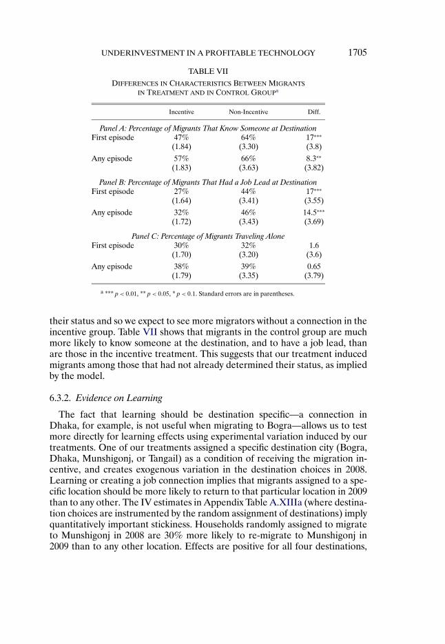
UNDERINVESTMENT IN A PROFITABLE TECHNOLOGY 1705
TABLE VII
DIFFERENCES IN CHARACTERISTICS BETWEEN MIGRANTSIN TREATMENT AND IN CONTROL GROUPa
Incentive Non-Incentive Diff.
Panel A: Percentage of Migrants That Know Someone at DestinationFirst episode 47% 64% 17∗∗∗
(1.84) (3.30) (3.8)
Any episode 57% 66% 8�3∗∗
(1.83) (3.63) (3.82)
Panel B: Percentage of Migrants That Had a Job Lead at DestinationFirst episode 27% 44% 17∗∗∗
(1.64) (3.41) (3.55)
Any episode 32% 46% 14�5∗∗∗
(1.72) (3.43) (3.69)
Panel C: Percentage of Migrants Traveling AloneFirst episode 30% 32% 1.6
(1.70) (3.20) (3.6)
Any episode 38% 39% 0.65(1.79) (3.35) (3.79)
a ∗∗∗p< 0�01, ∗∗p< 0�05, ∗p< 0�1. Standard errors are in parentheses.
their status and so we expect to see more migrators without a connection in theincentive group. Table VII shows that migrants in the control group are muchmore likely to know someone at the destination, and to have a job lead, thanare those in the incentive treatment. This suggests that our treatment inducedmigrants among those that had not already determined their status, as impliedby the model.
6.3.2. Evidence on Learning
The fact that learning should be destination specific—a connection inDhaka, for example, is not useful when migrating to Bogra—allows us to testmore directly for learning effects using experimental variation induced by ourtreatments. One of our treatments assigned a specific destination city (Bogra,Dhaka, Munshigonj, or Tangail) as a condition of receiving the migration in-centive, and creates exogenous variation in the destination choices in 2008.Learning or creating a job connection implies that migrants assigned to a spe-cific location should be more likely to return to that particular location in 2009than to any other. The IV estimates in Appendix Table A.XIIIa (where destina-tion choices are instrumented by the random assignment of destinations) implyquantitatively important stickiness. Households randomly assigned to migrateto Munshigonj in 2008 are 30% more likely to re-migrate to Munshigonj in2009 than to any other location. Effects are positive for all four destinations,

1706 G. BRYAN, S. CHOWDHURY, AND A. M. MOBARAK
FIGURE 4.—Migration experience in 2008 by re-migration status in 2009.
which is evidence in favor of location-specific learning, or the accumulation ofconnections at the destination being an important driver of migration behav-ior.
Our model also suggests that some induced migrants should discover thatthey are bad migrators, while some discover that they are good. Among reg-ular migrants, however, our model predicts no such effects—only householdsthat know they are good at migrating should migrate in the control group. Fig-ure 4 shows evidence consistent with this. In the treatment groups (credit orcash), those that chose to re-migrate in 2009 had a significantly better migra-tion experience in 2008 than those who chose not to re-migrate. In the controlgroup, however, we see no such effect.
6.4. Subsistence
Our model postulates that households may not migrate because they areclose to subsistence, and risk falling below subsistence if they have a bad mi-gration outcome. We can study the distribution of expenditures and caloricintake to examine whether this setup is warranted.
The Bangladesh Bureau of Statistics classifies a person as ultra-poor if theyconsume less than 1605 calories, and it is usually thought that something be-tween 600 and 1000 calories are required just to survive. Based on the pricescollected in our baseline survey, and assuming very basic calorie composition,we estimate that it would cost about 660 Taka per person per month to meet theultra-poor level, 450 Taka to consume 1000 calories, and 250 Taka to consume

UNDERINVESTMENT IN A PROFITABLE TECHNOLOGY 1707
600 calories. Comparing these figures to the distribution of per capita expendi-tures in our sample presented in Appendix Figure A.1, we see that a substan-tial portion of households are close to subsistence. Appendix Figure A.2 showsdirectly the histogram of calories per person per day in the control group inour December 2008 follow-up. Many households in the control group can becharacterized as “close to subsistence” in terms of caloric intake. Comparingthe treatment and control histograms, we again see that our treatment movedmany people from a subsistence level of consumption (of 800–1300 caloriesper person per day) to a comfortable level exceeding 2000 calories per personper day.
Our model suggests that if aversion to the risk of falling below subsistenceis an important deterrent to migration, then: (a) people close to subsistenceshould not be migrating in the control group, and (b) our treatment shouldhave the largest effect on households that are close to subsistence: they shouldbe the ones induced to migrate by our incentive. The three panels in Figure 5show strong evidence in favor of these two claims graphically and in a regres-sion. We measure subsistence as the proportion of total household expendi-tures devoted to food.32 The regression and the graphs show that those closerto subsistence are significantly less likely to migrate in the control group, andtheir migration decisions respond most strongly to the treatment.
6.5. Does the Model Rationalize Responses to All Treatments?
The model allows us to understand the impact of specific treatments de-signed to help households accumulate sufficient cash on hand to engage inprofitable migration. In this section, we compare the impacts of several poten-tial policies on which we have collected data.
First, as noted above, our initial treatments included both cash and credit in-centives. In practice, these two incentives have approximately the same impacton the migration rate. Here we argue that this finding is consistent with themodel, if credit is seen as incorporating a limited liability aspect. An assump-tion of limited liability is consistent with the fact that only 80% of householdsrepaid the loan.
32The ratio of food to total expenditures has less measurement error than caloric intake ortotal expenditure as a measure of proximity to subsistence because (a) caloric requirements varygreatly across families with different age, gender compositions, and activity levels, and (b) pricesused to calculate expenditures vary across families, introducing noise (which is eliminated whencomputing the ratio). We therefore prefer the ratio measure for our regression, even thoughwe describe subsistence in our sample in Appendix Figure A.2 using more intuitive measureslike calories consumed. The concept behind this measure is motivated by the literature on foodconsumption, which shows that the elasticity of calories to income is modest even among the verypoor (e.g., Subramanian and Deaton (1996)). Jensen and Miller (2008) used a similar measure ofsubsistence.

1708 G. BRYAN, S. CHOWDHURY, AND A. M. MOBARAK
Panel B: Migration Decision as a Function of Baseline Subsistence
Incentivized −0.223(0.186)
Ratio of food expenditure over total expenditure round 1 −0�828∗∗∗
(0.211)
Interaction: Ratio of food to total ∗ Incentivized 0�566∗∗
(0.246)
Constant 0�686∗∗∗
(0.189)
Observations 1856R-squared 0.189
aRobust standard errors in parentheses, clustered by village. ∗∗∗p < 0�01, ∗∗p < 0�05, ∗p <0�1. The dependent variable is “Migration,” a binary variable equal to 1 if at least one mem-ber of the household migrated and 0 otherwise. Additional treatment variables included but notshown were: random assignment into individual or group migration and random assignment bymigration destination. Additional controls were number of adult males at the baseline, num-ber of children at the baseline, past migration dummy, lacked access to credit, borrowing, totalhousehold expenditures per capita measured at baseline, and social network support measuredat baseline.
FIGURE 5.—Heterogeneity in migration responsiveness to treatment by subsistence level.
We can capture the limited liability effect of credit by noting that householdshave to have a reason to repay their loans. Let M(x) = B(x− F) if the house-hold is a bad migrator, and M(x) = G(x) if the household is a good migrator,

UNDERINVESTMENT IN A PROFITABLE TECHNOLOGY 1709
FIGURE 5.—Continued.
and consider a household that has a loan of value L and is required to repay Z.The household will repay the loan if and only if
M(x−Z)≥M(x+L)− P�
where P is a utility cost of punishment by the lender. P is assumed to be stateindependent, as the punishment should reflect the long-run value of credit tothe household. This setup is easily able to generate the experimental findingthat cash and credit have the same impact. The cash treatment differs fromcredit treatment in making a payout when the migrator is good, but this hasa low value, as it occurs when consumption would be high anyway. The creditcontract also differs from cash because it costs P to use the limited liability,which provides insurance in the bad state. This cost P is, however, very smallrelative to the benefit because the household that uses it is close to subsistence.Both these arguments imply that, for concave enough utility functions, the cashand credit have almost identical effects, a fact which we can also demonstratein our calibrations below.
Second, as noted above, we returned in 2011 and implemented new treat-ments. One of these treatments was an unconditional credit contract of thesame size as the conditional credit transfer. Our motivation for this experimentwas to rule out the possibility that households were merely cash constrained.Our model implies that the credit incentive should have a larger impact, asit only increases household’s utility when it migrates, while the unconditional

1710 G. BRYAN, S. CHOWDHURY, AND A. M. MOBARAK
credit also increases the payoff to staying at home.33 This is an implication ofany model in which a household weighs the returns to migration relative toother possible uses of the money, but is not an implication of a model wherethe household knows that migration is profitable, but simply cannot afford it.The results of this experiment are shown in the first column of Table V, andindicate that, consistent with our model but inconsistent with a cash constraintmodel, the unconditional transfer has a smaller impact than the conditionaltransfer.34
6.6. Summary of Qualitative Tests
In summary, both descriptive and experimental analyses of the data indi-cate that our model accurately captures many key aspects of the environment:background income is volatile, migration is risky, savings is high, and migra-tion is an experience good. The model also (qualitatively) rationalizes mostof the data coming from our experiment: the fact that credit and cash havesimilar sized impacts, the fact that the incentive was most effective for thosethat are close to subsistence, the relative impacts of unconditional and condi-tional transfers, and the response to the insurance treatment. What remains tobe seen, however, is whether the model brings all of these ingredients of themigration decision together in a way that can quantitatively account for themagnitude of the experimental effects.
7. QUANTITATIVE CALIBRATION OF THE MODEL
Our quantitative exercise will use the data to calibrate all the free parame-ters of the model except risk aversion. We then ask what level of risk aversionwould be required to match key aspects of the data. Table VIII shows the pa-rameters we use for the quantitative exercise. In all cases, we have erred on theside of allowing the model to generate the experimental estimates. This choicereflects the fact that we will ultimately argue that the model in its basic formis not able to rationalize the experimental estimates. Our interpretation of thisresult is that the qualitative evidence above suggests that the model capturesseveral key aspects of the setting, and gives guidance to where we would ex-pect to be able to replicate our experimental findings. However, because themodel fails to quantitatively explain the experimental results, there remainssome element of household behavior or the environment that our model doesnot capture, which would result in the observed under-migration. We thereforeview the model as providing a starting point for future work on what preventsinvestments in profitable technologies like seasonal migration.
33In terms of the discussion in Appendix B, the conditional credit payment moves only the V M
curve, while the unconditional credit raises the V N curve as well.34Although we presented the products in a similar way, if household perceptions of repay-
ment requirements varied between the conditional and unconditional loans, that may also leadto differential take-up.

UNDERINVESTMENT IN A PROFITABLE TECHNOLOGY 1711
TABLE VIII
PARAMETERS USED FOR CALIBRATION
Parameter Calibration Notes
u(c) (c−s)1−σ
1−σHARA utility function
s 250 Taka per hh memberper month
Enough for about 600 calories per hhmember per month
πG 0.5 The portion of induced migrants thatre-migrate
F 250 Taka per hh memberper month
600 Taka for bus fare, plus 6 days offoregone labor at 60 Taka per day.Spread over 4 hh members
m 550 per household memberper month
Solution to: πG(m+ I)= 350 where350 is our LATE estimate and I isthe size of our incentive
μ(y) N(700�70) per household memberper month
Designed to look like the distributionof the bottom half of the population
Time period 6 months We assume the choice to migrate canbe made after planting for either ofthe agricultural seasons
δ 0.99
I (incentive size) 200 Taka per household member Assumes a households size of 4
Three calibration choices deserve special mention. First, we assume thatthere are two opportunities to migrate each year (or two time periods peryear): one after each planting season. This means that a time period for thepurpose of the model should be thought of as half a year. Second, we assumethat the cost of migration, F , must be borne over 1 month, so that consump-tion when migration is bad is very low. This reflects the fact that most house-holds earn money during the monga season and use it to pay for consump-tion. Credit-constrained households will have to pay for migration out of thisincome, reflecting the possibility that the subsistence constraint binds, and thehousehold has no choice but to finance migration out of contemporaneous con-sumption. Third, we assume that income at home is distributed N(700�70).35
This is an attempt to estimate the income distribution of the lowest 50% ofhouseholds in the sample. We argue that the results of this section are notsensitive to this choice.
35The use of the normal distribution implies that the model does not in fact contain a povertytrap: as time goes to infinity, all households will eventually receive a shock so large that theydecide to migrate. In practice, this is not a problem for our calibrations for two reasons. First,we truncate the distribution in the upper tail because we have to make a discrete approximationto make the calibration feasible. Second, we work with short time periods—always less than 20years—implying that this theoretical possibility does not seem important in practice.

1712 G. BRYAN, S. CHOWDHURY, AND A. M. MOBARAK
We undertake two different exercises. First, we use the model to determinefour cutoff points—x, xI , xC , and xUCT : the amount of cash on hand required tomigrate with no intervention, with our cash incentive, with a credit incentive,and with an unconditional cash transfer, respectively. We then match theselevels of cash on hand to the histogram of consumption levels in the controlgroup and ask what portion of the distribution lies between the relevant boundsto estimate the set of migrants that our treatments are predicted to induce. Forexample, we consider the density of households consuming between xI and xto estimate the portion of households that would be induced to migrate byour incentive. This exercise essentially ignores the repeat migration effect andlearning, or the possibility of saving up to migrate (although households doconsider the benefit of repeat migration when making their choices).
Our second exercise is to ask what portion of households can still be in-duced to migrate after t periods. A household is “induceable” in period t ifit does not yet know its type. In the model, only induceable households willbe affected by our migration incentive, as other households will have alreadydetermined their status as good or bad migrators. For this exercise, we makeuse of the assumed background income distribution to determine the proba-bility of a household crossing the migrating threshold x in each period. If thenumber of induceable households is very low after only a small number of timeperiods, then the model cannot rationalize the experimental results.36
Here we present results from calibrating the full model; Appendix E (inSupplemental Material (Bryan, Chowdhury, and Mobarak (2014))) presentsfurther discussion. The left panel of Figure 6 shows the portion of migrantsthat would be induced assuming no repeat migration and the right panel showsthe number of induceable migrants as a function of the time period. The leftpanel shows that, ignoring the dynamic effects of migration, the model predictsthat, with a risk aversion of σ ≈ 1�5, our incentive would induce about 20%of households to migrate—consistent with our experimental findings. Further,consistent with our experimental results, the cash and credit incentives havethe same effect. However, while the unconditional cash transfer has a smallereffect, as predicted, at low levels of risk aversion the UCT continues to induceabout 17% of the population to migrate, higher than observed in the data.Despite this quantitative inconsistency, this form of the model is broadly con-sistent with our experimental results.
The right hand panel, however, shows that once we allow for savings up andrepeat migration, the model is no longer able to rationalize the data. With arisk aversion level of about 11, 40% of the population is induceable after 8 sea-sons (or 4 years), which corresponds to a 20% treatment effect if the model
36In all the results presented below, we depart slightly from the baseline model and assumethat households that migrate and are determined to be bad migrators are also induceable. Thiserrs on the side of allowing the model to fit the data. See also the discussion in footnote 21.

UNDERINVESTMENT IN A PROFITABLE TECHNOLOGY 1713
FIGURE 6.—Full model with buffer stock savings and possibility of saving up for migration.

1714 G. BRYAN, S. CHOWDHURY, AND A. M. MOBARAK
applies to the poorest half of the sample. If we allow 10 prior years of migra-tion activity, the model suggests that even σ ≈ 20 is insufficient to rationalizethe results.37 We discuss plausible values for risk aversion in the next section,but believe that most scholars would think 20 to be implausible, especially inour model, where the subsistence constraint means that behavior will exhibiteven more risk aversion. Because it seems reasonable to assume that house-holds in our treatment areas have faced a similar migration choice for sometime, and quite reasonably for 10 prior years, we conclude that the modelcannot quantitatively account for our experimental findings: there should notbe large numbers of people living in the villages who can be induced to mi-grate.
These results are robust to our assumption regarding the distribution ofincome. We have simulated the right panel of Figure 6 for standard devia-tions from 40 to 140, and the results are almost identical. As discussed in Ap-pendix B, there are several impacts of increasing the degree of backgroundrisk, and the simulations suggest that, for our parameter values, these effectscancel each other out.
We can also use the model to ask whether the observed level of savings isconsistent with the model. For a risk aversion level of 0.5, the model predictsa household will hold, on average, 1500 Taka in savings, which is roughly inline with what we see in the data. For higher levels of risk aversion, however,the model predicts far more savings than we observe: at a risk aversion levelof 5, predicted average savings is close to 3000 Taka, and at σ = 10 we predictsavings of nearly 5000 Taka. It is not possible to match both the level of savingsand the responses to the migration treatments at any given level of assumedrisk aversion.
In Appendix E, we discuss two alternative forms of the model: first, a com-pletely static model, where households do not save for migration and do notconsider the benefits of ongoing migration when they make their initial migra-tion choice—that is, they are myopic past the current migration period; andsecond, a model in which we assume that there is no savings, but allow house-holds to be forward looking. The results allow us to better understand whythe model cannot match the data and reveal two main results. First, forward-looking behavior is very important in driving the results: if the households arenot forward looking and do not save, then the model is able to match the data,but if the households are forward looking and cannot save, then we cannotmatch the experimental results without risk aversion levels of greater than 5,
37These results assume that households begin time with no assets and the lowest possible in-come shock. We use the model to generate policy functions as well as cutoff values. We thensimulate the model for 10,000 households and ask what portion of those 10,000 households hasnot migrated after t periods. Another way to summarize the results is to say that the distribu-tion of cash on hand implied by the model is insufficiently close to subsistence to support theexperimental results.

UNDERINVESTMENT IN A PROFITABLE TECHNOLOGY 1715
which may be implausibly high. Second, allowing savings has two partially off-setting effects. On one hand, savings reduces the value of migration because itallows the household to self-insure through buffering, reducing the need to ex-periment with migration. This effect means that, in a myopic model, allowingsavings allows us to more easily rationalize the data. On the other hand, savingsallows households to save up to migrate. As we see above, once this effect isincorporated, it becomes extremely hard to rationalize the data—householdsshould be saving for an opportunity that is this profitable.
8. EXTENSIONS
While the qualitative evaluation of the model shows that households do save,that they respond to migration incentives in ways predicted by the model, andthat they perceive migration to be risky, the calibration exercise suggests thatto match the magnitudes of responses to our treatments, we have to extend themodel in some way. It could be that households underestimate the benefits ofmigration, or they are unable to save up for migration, or they are insufficientlyforward-looking. In this section, we briefly summarize extensions that we haveconsidered, and provide further details in Appendix F (in Supplemental Ma-terial). We do not have the data to determine conclusively which extensionsare the most important. We therefore see this section as an extended call formore work, and we provide some suggestions based on our model and data,regarding approaches that are unlikely to work. We consider a large numberof possibilities partly to highlight the uncertainty and the need for additionalexperimentation before moving to policy prescriptions.
The thrust of our calibration argument is that households would have to bevery risk averse to generate our data. However, if we allow σ to be very high,then the model can rationalize most of the data.38 The literature has not arrivedat a consensus on “reasonable” values for σ : Holt and Laury (2002) stated thatsomeone with σ > 1�37 should “stay in bed,” while papers in the equity pre-mium literature (e.g., Kandel and Stambaugh (1991)) argued that values ashigh as 30 may be reasonable. In our model, households are much more riskaverse than implied by their σ because they become infinitely risk averse asconsumption approaches the subsistence point. In circumstances analogous toours, Chetty and Szeidl (2007) showed that agents even in developed coun-tries become more risk averse with commitments for consumption. In futureresearch, it would be worth exploring at what point risk aversion should beconsidered to be a “mistake” that a policy maker should seek to address. Ifextreme risk aversion is akin to a behavioral bias, then adding conditions totransfers may improve a migrator’s utility over unconditional cash transfers.
38As we note above, however, high risk aversion is not a complete panacea, as it would implyvery high savings rates, which we do not observe in the data.

1716 G. BRYAN, S. CHOWDHURY, AND A. M. MOBARAK
Changing model parameters presents a second obvious way to improve thefit of the model. We have experimented with several different specifications ofthe returns to migration, including allowing for risk in m. This does not sub-stantially improve the ability of the model to fit the data. We also consideredthe effect of lowering the discount factor (δ) or allowing for depreciation ofthe status of being a good migrator. We considered only reasonable levels of δand depreciation consistent with the high re-migration rates, and while thesepossibilities allow for a better fit, high risk aversion levels are still required tomatch the experimental findings.
A third explanation is that migration is unpleasant and there is high non-pecuniary disutility from migration. We estimate the value of this disutilityfrom our data (see Appendix F for details), but this is unlikely to account forour experimental results. The central issue is that while high disutility may pre-vent migration, it would also reduce responsiveness to our interventions.
We also examined whether incorrect beliefs about the returns to migrationcould drive the results.39 To assess this possibility, we asked all migrants inboth treatment and control groups about how their migration experience, interms of time it took to find work and their earnings at destination, comparedto their expectations prior to migration. If households have biased beliefs, wewould expect that those in the control group, who were already migrating andhad a chance to learn, would have roughly correct beliefs, while those in thetreatment group would have beliefs biased toward the overly pessimistic.40 Re-sults presented in Appendix Table A.XIV are not consistent with biased be-liefs: treatment group migrants do not have significantly different beliefs fromcontrol group migrants.
The slightly different character of our results for the model with and withoutsavings points to the possible conclusion that it is savings behavior that is thereal anomaly (why are people not saving up to migrate?). Our sample house-holds may be savings constrained due to sharing norms (Jakiela and Ozier(2012)), or they may simply have no safe place to store things. This conclu-sion is consistent with recent research that demonstrates very large impacts ofsimple interventions that relax savings constraints (e.g., Dupas and Robinson(2013)). Two caveats should be mentioned, however. First, before citing savingsconstraints as the key issue, it is necessary to understand why households areable to buffer, but not to save up a lump-sum amount for migration. Second, aswe argue above, even without savings, forward-looking households should not
39One possible cause of bias is that non-migrators have access to incorrect information.McKenzie, Gibson, and Stillman (2007) argued that migrant households provide incorrect in-formation because they do not want to have to share resources, or job connections and accom-modation at the destination.
40To be clear, it is not evidence of incorrect beliefs that some people found the experienceworse than anticipated; this is perfectly consistent with an ex post statement about an ex anterisky event. The prediction of biased beliefs is that those in the treatment should be more likelyto have done better than expected.

UNDERINVESTMENT IN A PROFITABLE TECHNOLOGY 1717
be induceable in great numbers.41 There is, therefore, a need to understandmore than just savings constraints; we must also understand why householdsact as though they are not aware of the full benefits of migration.
Another related avenue to consider may be the need to share risk and solvepublic goods problems in general. Risk sharing networks not only constrainsavings; they may also deter profitable investments (e.g., Lewis (1955)). Mi-grating away may undermine network ties, and this may be a hidden cost ofmigration (Munshi and Rosenzweig (2009)).
Finally, many models that fall under the rubric of behavioral economicscould be used to explain the results. In this area, we are particularly waryof making pronouncements without data, as there are many different pos-sible explanations. Here, we mention just two models that have been ap-plied to developing country contexts. First, the quasi-hyperbolic discountingmodel of Laibson (1997) can likely be applied to rationalize the data forsome values of β. The version of this model discussed in Duflo, Kremer, andRobinson (2011) provided an explanation for low savings. The version of thismodel discussed in Banerjee and Mullainathan (2010) can explain why house-holds do not undertake profitable investments. Second, Koszegi and Rabin’s(2006) model of reference dependence can likely rationalize the data. Thatmodel provides a non-self-control based explanation for the fact that house-hold find themselves to be perpetually without the money they need to in-vest: households adjust their expected consumption in response to shocks andthen assess the costs of investments relative to this expected consumptionlevel.
In summary, there are numerous avenues that could be pursued to get abetter quantitative accounting of the data generated by our experiment. Wehave noted just a few. We are currently working on isolating which factors aremost relevant in other settings where seasonal migration is relevant.
9. CONCLUDING REMARKS
We conducted a randomized experiment in which we incentivized house-holds in a famine-prone region of Bangladesh to send a seasonal migrant toan urban area. The main results show that a small incentive led to a large in-crease in the number of seasonal migrants, that the migration was successfulon average, and that households given the incentive in one year continued tobe more likely to migrate in future years. These results bolster the case madeby Clemens, Montenegro, and Pritchett (2008), Rosenzweig (2006), Gibsonand McKenzie (2010), Clemens (2011), Rodrik (2007), and Hanson (2009)that offering migration opportunities has large effects on welfare, even rela-
41This is shown in Appendix Figure A.7 (see Supplemental Material).

1718 G. BRYAN, S. CHOWDHURY, AND A. M. MOBARAK
tive to other promising development interventions in health, education, trade,or agriculture. The literature largely focuses on international migration, andwe show that the returns to internal migration—a much more common, butunderstudied phenomenon42—are also large.
We argue that the results are qualitatively consistent with a simple (ratio-nal) model of a poverty trap where households that are close to subsistenceface a small possibility that migrating will turn out badly, leaving householdconsumption below subsistence. The model helps us to understand the typesof situations in which we would expect incentive and insurance policies to leadto long-term benefits as observed in our experiment. We should look for sit-uations in which the investment is risky, that risk is individual specific, andwhere the utility cost of the downside risk is large (e.g., the household is closeto subsistence). These predictions also provide an answer to the puzzle thatmotivated the entire project: why does Rangpur—the poorest region of thecountry that regularly faces a seasonal famine—have a lower out-migrationrate compared to the rest of Bangladesh? This can also explain other pecu-liar migration patterns noticed in the literature—the lower out-migration rateamong poorer Europeans (Hatton and Williamson (1998)) and poorer SouthAfricans (Ardington, Case, and Hosegood (2009)).
Our quantitative work implies that we cannot provide a fully satisfying ex-planation for why people in Rangpur had not saved up to migrate.43 We aretherefore hesitant to draw policy implications from our research. However, itis clear that the migration support programs we implement help some Rangpurhouseholds cope with the monga famine, and appear more cost-effective thansubsidizing food purchases on an ongoing basis, which is the major anti-faminepolicy tool currently employed by the Bangladesh government (Governmentof People’s Republic of Bangladesh (2005), Khandker, Khaleque, and Samad(2011)). Two important caveats are that our research does not capture long-term psychological and social effects of migration, and the scale of our ex-periment does not permit us to analyze potential adverse general equilibriumeffects in destination labor markets if the government were to contemplatescaling up such a program.44
42There were 240 times as many internal migrants in China in 2001 as there were internationalmigrants (Ping (2003)), and 4.3 million people migrated internally in the 5 years leading up to the1999 Vietnam census, compared to only 300,000 international migrants (Anh (2003)).
43Several other papers document very high rates of return to small capital investments in de-veloping countries (Udry and Anagol (2006), de Mel, McKenzie, and Woodruff (2008), Bandiera,Barankay, and Rasul (2011), Duflo, Kremer, and Robinson (2011), Fafchamps, McKenzie, Quinn,and Woodruff (2011)), and this literature must also confront the same question of why householdsdo not save to invest in these high-return activities.
44There is mixed evidence in the literature on whether these effects are substantial (Ottavianoand Peri (2012), Borjas (2003), Borjas and Katz (2007), Card (2009)). Moreover, general equilib-rium effects may be positive in net, if spillover benefits at the origin exceed external costs at thedestination. Migrants form a much larger part of the village economy at the origin compared tothe destination urban economy.

UNDERINVESTMENT IN A PROFITABLE TECHNOLOGY 1719
If there are net efficiency gains, this is likely because our intervention mit-igates the spatial mismatch between where people live, and where jobs areduring the pre-harvest months. This approach may be of relevance to othercountries that face geographic concentrations of poverty, such as northernNigeria, eastern islands of Indonesia, northeast India, southeast Mexico, andinland southwest China (Jalan and Ravallion (2001)). More generally, provid-ing credit to enable households to search for jobs, and aid spatial and seasonalmatching between employers and employees, may be a useful way to augmentthe microcredit concept currently more narrowly focused on creating new en-trepreneurs and new businesses.45 The potential efficiency gains raise an in-teresting question of why private sector entities do not profit by developingmechanisms that link migrants to employers in the city. To understand this, weinterviewed several employers in Dhaka. The employers reported that thereare in fact “labor sardars” who bring migrant workers to Dhaka, but the processis fraught with uncertainty and risk. Migrants have to be paid the one-way busticket and some salary in advance, but it is difficult to enforce any long-termcontract if they disappear and choose to go work elsewhere after the transitcost is paid.
APPENDIX A: DESCRIPTION OF 2008 TREATMENTS
Out of the 100 villages selected to participate in the study, 16 (304 house-holds) were assigned to the control group, while the remaining 84 villages (1596households) were assigned to one of three treatments:
Information (16 villages/304 households): Potential migrants were providedwith information on the types of jobs available in each of four areas: Bogra,Dhaka, Munshigonj, and Tangail. In addition, they were told the likelihood offinding such a job, and the average daily wage in each job. This informationwas provided using the following script:
“We would like to give you information on job availability, types of jobs available, andapproximate wages in four regions—Bogra, Dhaka, Munshigonj, and Tangail. They arenot in any particular order. NGOs working in those areas collected this information at thebeginning of this month.Three most commonly available jobs in Bogra are: (a) rickshaw-pulling, (b) construc-tion work, (c) agricultural labor. The average wage rates per day are Tk. 150 to 200 forrickshaw-pulling, Tk. 120 to 150 for construction work, and Tk. 80 to 100 for agriculturallaborer. The likelihood of getting such a job in Bogra is medium (not high/not low).Three most commonly available jobs in Dhaka are: (a) rickshaw-pulling, (b) constructionwork, (c) day labor. The average wage rates per day are Tk. 250 to 300 for rickshaw-pulling,Tk. 200 to 250 for construction work, and Tk. 150 to 200 for day laborer. The likelihood ofgetting such a job in Dhaka is high.
45With credit contracts, it may be difficult to collect regular repayment from migrants whomove away, but one of the world’s largest micro-credit NGOs, BRAC, has recently introducedcredit programs to finance even international migration.

1720 G. BRYAN, S. CHOWDHURY, AND A. M. MOBARAK
Three most commonly available jobs in Munshigonj are: (a) rickshaw-pulling, (b) landpreparation for potato cultivation, (c) agricultural laborer. The average wage rates per dayare Tk. 150 to 200 for rickshaw-pulling, Tk. 150 to 160 for land preparation, and Tk. 150to 160 for agricultural laborer. The likelihood of getting such a job in Munshigonj is high.Three most commonly available jobs in Tangail are: (a) rickshaw-pulling, (b) constructionwork, (c) day laborer in brick fields. The average wage rates per day are Tk. 200 to 250 forrickshaw-pulling, Tk. 160 to 180 for construction work, and Tk. 150 to 200 for brick fieldwork. The likelihood of getting such a job in Tangail is medium (not high/not low).Based on the above information, would you/any member of your family like to go to anyof the above locations during this monga season? If so, where do you want to go? Notethat the job market information given above might have changed or may change in thenear future and there is no guarantee that you will find a job, and we’re just providing youthe best information available to us. Note also that we or the NGOs that collected thisinformation will not provide you with any assistance in finding jobs in the destination.”
Cash (37 villages/703 households): Households were read the same script onjob availability as given above, and were also offered a cash grant of Tk. 600conditional on migration. This money was provided at the origin prior to mi-gration, and was framed as defraying the travel cost (money for a bus ticket).Migrants had an opportunity to receive Tk. 200 more if they reported to us atthe destination.
Credit (31 villages/589 households): Households were read the same script onjob availability as given above, and were also offered a zero interest loan ofTk. 600 conditional on migration. This money was provided at the origin priorto migration, and was framed as defraying the travel cost (money for a busticket). Migrants had an opportunity to receive Tk. 200 more if they reportedto us at the destination. Households were told that they would have to pay backthe loan at the end of the monga season.
APPENDIX B: THEORY APPENDIX
In this appendix, we describe the behavior of agents in our baseline modelusing the value functions, policy functions, and simulated time series ofchoices. The appendix documents the facts about the model presented in Sec-tion 5.1.
Appendix Figure A.3 provides plots of two value functions, both for house-holds that have never migrated before. The first function shows the value to ahousehold that is forced to migrate in this period:
VM(x) = πGG(x)+ (1 −πG)B(x− F)�
The second function shows the value to a household that decides not to mi-grate in this period:
VN(x)= maxc≤x
[u(c)+ δ
∫S
V(ys +R(x− c)
)dμ(s)
]�

UNDERINVESTMENT IN A PROFITABLE TECHNOLOGY 1721
As is generally the case, VM crosses VN once from below. This implies a cut-off level of cash on hand x: for cash on hand below x, the household doesnot migrate; for cash on hand greater than x, the household does migrate. Be-cause the two value functions cross, the value V is not convex, which impliesthat the household would be risk loving at levels of cash on hand close to x.We do not allow households any kind of randomization that would help themtake advantage of this non-convexity—this is a feature of most poverty trapmodels. These issues are explored in detail in Vereshchagina and Hopenhayn(2009).
Appendix Figure A.4 displays typical policy functions—consumption as afunction of cash on hand—for the model. The first policy function shows con-sumption for a household that knows it is bad at migrating (cB), and the sec-ond for a household that has never migrated, but that we restrict to not mi-grate in the current period (cM). At low levels of cash on hand, both policyfunctions lie on the 45 degree line—the household spends all that it can. Ascash on hand rises, the household that knows it is a bad migrator begins tobuffer, consuming less than cash on hand and saving some money to smoothlater consumption. This is the standard result following Deaton (1991). Ini-tially, the household that can migrate does the same thing and the two policyfunctions lie on top of each other. As cash on hand approaches x, however, cMfalls below cB: the household that can migrate begins to save up for migration.Thus, the saving of a potential migrator can be divided into two parts: buffer-ing, and saving up for migration. The figure shows that, for some parametervalues, consumption is not a monotone function of cash on hand, a result thatis consistent with the findings of Buera (2009). As cash on hand rises past x, cMcontinues to lie below cB: we have constrained the household not to migratein this period, so it continues to save in the hope of migrating next period.Finally, there is a level of cash on hand past which cM > cB—the householdthat has never migrated knows that it can migrate next period and it is con-sequently richer (in expectation) than the household that knows it is bad atmigrating.
We are not interested in general results as t → ∞, but rather in the be-havior over real-world time periods. This behavior is inherently stochastic andbest understood by looking at simulations. Appendix Figure A.5 shows sim-ulations of cash on hand and consumption for two households with differentstarting levels of cash on hand (wealth). Both households are assumed to begood migrators. The panel on the left shows cash on hand and the right showsconsumption. The cash on hand simulation shows that the wealthier house-hold quickly saves enough to cross the migration threshold, x. After crossingthe threshold, cash on hand spikes as the household discovers that it is a goodmigrator. The poorer household never migrates. The consumption simulationshows that the wealthier household consumes less initially—as it saves up—butafter crossing the migration threshold, has a higher consumption level. In gen-eral, our simulations show that households with a lower mean income (Eμy)

1722 G. BRYAN, S. CHOWDHURY, AND A. M. MOBARAK
or with a lower starting cash on hand are less likely to cross the threshold forany finite time period, indicating a kind of poverty trap. It is this poverty trapthat can potentially explain our experimental results: a portion of householdsare stuck in a low-income situation in which they cannot migrate, but a smallintervention can push them to experiment with migration, with potentially highreturns.
We can also use the model to consider other comparative statics. Risk aver-sion appears intuitively linked to aversion to experimentation, but the modelsuggests that the relationship is more complicated. Simulations show that anincrease in risk aversion has three effects. First, increasing risk aversion in-creases the cost of experimenting with migration and tends to increase x andthus reduce the propensity to migrate. Second, as risk aversion increases, thereturn to migration increases because migration can be seen as a risk mitigationstrategy. Third, for many utility functions (including the one we use for simu-lations), absolute prudence increases with risk aversion.46 As a consequence,as risk aversion increases, the household engages in more buffer stock saving,implying that the household is more likely to cross any given threshold level ofcash on hand. We have not sought a general characterization of which effectdominates, but do observe all three effects in our simulations. Similar effectsapply to an increase in the riskiness of income. On the one hand, a riskierincome means more background risk and, therefore (for specific utility func-tions), effectively an increase in risk aversion. On the other hand, more riskmeans more buffer stock savings.
APPENDIX C: DESCRIPTION OF TREATMENTS IN 2011
In 2011, we conducted one more round of randomized interventions in thesame sample of 1900 households (in 100 villages), plus 247 new households in13 new randomly selected villages from the same two districts (Kurigram andLalmonirhat). The treatments (most of which encouraged migration, like the2008 experiments) were randomized at the village level. They were offered inFebruary 2011, just before the onset of the 2011 “mini-monga season,” whichis the pre-harvest lean season associated with the lesser of the two annual riceharvests. The treatments were therefore designed to encourage migration dur-ing this lean season. The same organization as in 2008—PKSF, and their localNGO partners—implemented the treatments. We collected follow-up data onall households in 133 villages in July–August 2011.
Controls: All 16 Control villages from the 2008 experiments were retainedas a control group in 2011. We also chose not to intervene again in 19 villages
46The coefficient of absolute prudence is defined as u′′′(x)u′′(x) . See Kimball (1990) for a definition
of prudence and the relationship to precautionary savings and concepts of risk aversion includingdecreasing absolute risk aversion.

UNDERINVESTMENT IN A PROFITABLE TECHNOLOGY 1723
that were offered the credit treatment in 2008. These 19 villages are labeled“Impure Control” in the regression table, and they allow us to study the long-run effects of offering migration credit in 2008.
Credit conditional on migration: Sample households in 15 villages receivedthe same zero-interest loan conditional on a household member migrating, asoffered in 2008. The credit amount was raised to Tk. 800 (∼US$10.8) to reflectinflation in the cost of travel since 2008. Households were required to pay backin a single installment in July, at the end of the lean season.
Unconditional credit: To test one of the implications of our model, we offeredan unconditional zero-interest loan of Tk. 800 to sample households in 15 vil-lages. The loan repayment terms were the same as the conditional credit, andno conditionality was attached to the loan.
Conditional credit with destination rainfall insurance: Sample households in24 villages were offered the same zero-interest Tk. 800 (∼US$10.8) credit con-ditional on migration, but the repayment terms were conditioned on rainfalloutcomes in one popular migration destination: Bogra. Too much rainfall (andflooding) is a risk in Bangladesh, and can lower migrant earnings, particu-larly for outdoor work like rickshaw-pulling and construction site work. Wepurchased 10 years of daily rainfall data from the local meteorological de-partment, imputed the probability distribution of rainy days during the pre-harvest migration period, and calculated the actuarially fair insurance pre-mium and payoff amounts. Our loan contract specified that if rainfall in Bo-gra for March/April 2011 remained “normal” (4 days or less), the migrantswould have to pay back Tk. 950 (∼US$12.83). For 5–9 days of rainfall, the re-payment requirement would be Tk. 714 (∼US$9.64). For 10 or more days ofrainfall, the repayment requirement was Tk. 640 (∼US$8.64). The amountswere chosen to make the insurance contract actuarially fair, given historicalrainfall data.
Note that this is a loan contract, but the repayment rules introduce a featureof index insurance against too much rainfall.47 The treatment design takes ad-vantage of the fact that the contract offers differential basis risk for householdsthat differ along identifiable baseline characteristics: those who had a propen-sity for traveling to Bogra, and non-farmers. Basis risk from the index contractis lower for these two groups.
All treatments described above were proportionally balanced across the In-formation, Cash, and Credit treatments from 2008 (and Control villages from2008 were retained as long-term controls as described above). In some othersample villages from 2008, we conducted other treatments that are not relevantfor the analysis conducted in this paper, and we therefore do not discuss thosetreatments here.
47Note that the contract can be explained to borrowers like a standard credit contract, and theinsurance feature is only introduced because the credit repayment is state contingent. This helpsto avoid confusion about the concept of insurance (Gine and Yang (2009)).

1724 G. BRYAN, S. CHOWDHURY, AND A. M. MOBARAK
APPENDIX D: APPENDIX TABLES AND FIGURES
TABLE A.I
FIRST-STAGE: MIGRATION AS A FUNCTION OF TREATMENTS IN 2008a
Migration in 2008
Cash 0�169∗∗∗ 0�178∗∗∗
(0.045) (0.044)
Credit 0�164∗∗∗ 0�165∗∗∗
(0.044) (0.044)
Info −0.012 −0.000(0.044) (0.044)
Sub-district fixed effects? Yes YesAdditional controls? No Yes
Observations 1868 1824R-squared 0.101 0.1451st F-test 12.74 12.581st p-value 0.000 0.0001st partial R2 0.027 0.028
aRobust standard errors in parentheses, clustered by village. ∗∗∗p < 0�01, ∗∗p <0�05, ∗p< 0�1. Table displays first-stage results for the regressions displayed in columns6–7, row 1, of Table III. First stage for other dependent variables varies slightly de-pending on the sample used (varies only if observations are missing). The dependentvariable is a binary variable equal to 1 if at least one member of household migrated.Additional controls included in column 2 are: household education, proxy for income(wall material), percentage of total expenditure on food, number of adult males, num-ber of children, lacked access to credit, borrowing, total household expenditures percapita measured at baseline, and subjective expectations about monga and social net-work support measured at baseline.

UNDERINVESTMENT IN A PROFITABLE TECHNOLOGY 1725
TABLE A.II
INTENSIVE AND EXTENSIVE MARGIN CHANGES DUE TO INCENTIVE (CASH OR CREDIT)a
2008 2009 2011
Total number of migration episodes per household 0�385∗∗∗ 0�186∗∗∗ 0.019(0.070) (0.071) (0.026)
Total number of migrants per household 0�190∗∗∗ 0�074∗∗ 0�071∗
(0.034) (0.035) (0.036)
Changes on Intensive MarginTotal number of migration episodes per household 0.111 0.110 −0.001
(among migrant households) (0.104) (0.069) (0.053)
Total number of migrants per household −0.017 −0.009 0.015(among migrant households) (0.023) (0.018) (0.015)
Total number of episodes per migrant 0.127 0.110 −0.021(0.097) (0.067) (0.041)
Days away per migrant per episode −11�722∗∗ −2.705 3�336∗∗
(5.283) (3.987) (1.432)
Male 0.016 −0.004 −0�010∗∗
(0.015) (0.007) (0.004)
Age 2�625∗∗ 0.128 −0.153(1.106) (1.012) (0.832)
Migrant is head of household 0�070∗∗ −0.027 −0.004(0.032) (0.028) (0.019)
aRobust standard errors in parentheses, clustered by village. ∗∗∗p < 0�01, ∗∗p < 0�05, ∗p < 0�1. Each coefficiententry in the table comes from a separate regression where the dependent variable (in column 1) is regressed on“incentivized” (cash and credit groups in 2008 and 2009; conditional, unconditional credit, cash, or rainfall insurancein 2011).

1726G
.BR
YA
N,S.C
HO
WD
HU
RY
,AN
DA
.M.M
OB
AR
AK
TABLE A.III
EFFECTS OF MIGRATION IN 2008 ON CONSUMPTION IN 2008; SENSITIVITY TO CHANGES IN DEFINITION OF HOUSEHOLD SIZEa
ITT
Dependent Variable: Cash Credit Info ITT IV OLS
Panel A: Household Size Is Based on Question Q7 in R2 Follow-Up Survey (“Status of Household Members”)Consumption of food 49�674∗∗ 48�292∗∗ 20.427 39�033∗ 222�288∗ −7.835
(23.752) (23.015) (36.787) (21.745) (124.365) (15.422)
Consumption of non-food 35�320∗∗ 28�121∗∗ 20.817 21�721∗∗ 122�929∗ 32�930∗∗∗
(14.941) (14.046) (18.860) (10.348) (63.274) (8.621)
Total consumption 104�162∗∗∗ 86�081∗∗∗ 41.620 75�234∗∗ 429�585∗∗ 61�339∗∗∗
(32.672) (31.318) (49.635) (30.031) (176.462) (20.343)
Total calories 120�927∗∗ 111�339∗∗ −66.444 148�964∗∗∗ 869�842∗∗∗ 102�951∗∗∗
(per person per day) (54.673) (51.398) (68.194) (42.735) (243.784) (38.129)
Panel B: Household Size Is Based on Question Q9 in R2 Follow-Up Survey (“Currently Present Members”)Consumption of food 50�506∗ 46�669∗ 5.063 46�219∗ 267�336∗∗ 67�936∗∗∗
(26.961) (26.185) (38.967) (23.648) (133.310) (17.226)
Consumption of non-food 29�778∗∗ 25�690∗ 18.536 18�774∗ 106�119∗ 45�519∗∗∗
(13.686) (13.495) (18.144) (9.917) (59.272) (9.152)
Total consumption 80�085∗∗ 71�211∗∗ 23.634 64�328∗∗ 368�937∗∗ 112�357∗∗∗
(31.663) (31.784) (49.575) (29.958) (171.948) (22.179)
Total calories 69.645 77.571 −117.409 130�875∗∗∗ 775�485∗∗∗ 218�266∗∗∗
(per person per day) (65.251) (62.278) (76.655) (48.946) (274.635) (41.640)
(Continues)

UN
DE
RIN
VE
STM
EN
TIN
APR
OF
ITAB
LE
TE
CH
NO
LO
GY
1727
TABLE A.III—Continued
ITT
Dependent Variable: Cash Credit Info ITT IV OLS
Panel C: Household Size Is Based on the Total Number of Household Members at the Time of the InterviewConsumption of food 56�019∗ 49�215∗ 21.065 42�498∗ 243�791∗ 80�573∗∗∗
(28.385) (27.493) (40.053) (24.070) (132.883) (16.898)
Consumption of non-food 32�313∗∗ 27�335∗∗ 25.281 17�586∗ 98�361∗ 49�524∗∗∗
(13.170) (12.594) (17.941) (9.593) (56.223) (8.738)
Total consumption 88�138∗∗ 75�440∗∗ 46.380 59�440∗ 337�769∗∗ 129�019∗∗∗
(34.016) (33.216) (51.202) (30.518) (170.467) (21.769)
Total calories 90.556 91.954 −69.585 125�294∗∗∗ 737�107∗∗∗ 252�609∗∗∗
(per person per day) (60.478) (56.772) (75.689) (46.656) (249.228) (40.847)
Panel D: Household Size Is Based on the Total Number of Household Members Present in the Last 14 DaysConsumption of food 65�320∗∗ 52�001∗ 16.532 50�952∗∗ 294�218∗∗ 114�443∗∗∗
(29.708) (29.165) (40.476) (24.395) (130.921) (17.779)
Consumption of non-food 37�317∗∗∗ 28�879∗∗ 22.655 22�246∗∗ 126�026∗∗ 63�824∗∗∗
(13.105) (12.307) (17.403) (9.709) (56.518) (9.154)
Total consumption 102�441∗∗∗ 79�753∗∗ 39.221 72�541∗∗ 415�549∗∗ 177�147∗∗∗
(35.327) (34.650) (51.050) (30.846) (167.430) (22.851)
Total calories 115�229∗ 97.084 −83.808 147�739∗∗∗ 872�820∗∗∗ 350�271∗∗∗
(per person per day) (65.440) (63.041) (77.209) (48.055) (243.244) (41.971)
(Continues)

1728G
.BR
YA
N,S.C
HO
WD
HU
RY
,AN
DA
.M.M
OB
AR
AK
TABLE A.III—Continued
ITT
Dependent Variable: Cash Credit Info ITT IV OLS
Panel E: Total Monthly Consumption per Household; No Adjustment to Household SizeConsumption of food 68.356 58.472 −29.407 78.084 454.672 −22.104
(125.876) (126.579) (171.409) (104.435) (584.120) (59.784)
Consumption of non-food 81�562∗ 53.790 60.009 39.126 219.877 41.280(41.239) (40.458) (48.636) (31.682) (179.086) (25.780)
Total consumption 149.230 108.306 30.727 114.917 660.329 15.572(143.280) (145.175) (203.232) (125.865) (701.793) (74.566)
Total calories −9.354 −21.278 −426.987 193.855 1169.733 22.695(279.707) (274.067) (342.132) (225.931) (1245.768) (166.249)
aThis table explores whether measurement error in migration dates and in household size net of migrants biases our estimates of the effects of migration on per capitaconsumption. We conduct a number of sensitivity checks below by varying the definition of household size (the denominator in the dependent variables measuring consumption).We conservatively assume that household members present in the house on the day of the interview were present for the entire prior month to consume the reported expenditures,since this variable is least likely to suffer from measurement error and coding problems. We compute this household size based on different questions in the survey (“who currentlylives in the household” as opposed to “who is present on the interview date”). Both ITT and IV results remain statistically significant, but slightly smaller (e.g., 130 or 125 caloriesrather than 142) in some specifications. Finally, even with the very conservative assumption that migrants never left, migration is estimated to increase consumption by 1169calories per household (or 292 calories per person, based on four household members) per day in the IV or 194 calories per household per day in the ITT. However, this lastresult, shown in panel E, is no longer statistically significant. Robust standard errors in parentheses, clustered by village. ∗∗∗p< 0�01, ∗∗p< 0�05, ∗p< 0�1.

UN
DE
RIN
VE
STM
EN
TIN
APR
OF
ITAB
LE
TE
CH
NO
LO
GY
1729
TABLE A.IV
EFFECTS OF MIGRATION BEFORE DECEMBER 2008 ON CONSUMPTION AMONGST REMAINING HOUSEHOLD MEMBERSa
ITT
Cash Credit Info ITT ITT IV IV OLS Mean
Panel A: 2008 ConsumptionCalories from protein 2�852∗ 2�588∗ −0.509 2�977∗∗ 2�657∗∗ 17�442∗∗ 15�573∗∗ 6�777∗∗∗ 46.51
(per person per day) (1.557) (1.571) (2.089) (1.287) (1.273) (7.064) (6.830) (0.992)
Consumption of meat 12�325∗∗ 6.577 8.163 5.618 5.599 31.857 34.302 3.905 28.26(5.489) (5.402) (6.667) (3.755) (3.726) (21.549) (21.399) (3.923)
Consumption of milk and egg −0.468 −1.365 0.026 −0.904 −1.318 −5.127 −7.237 1.764 13.06(2.256) (2.334) (2.401) (1.563) (1.544) (9.107) (9.052) (1.679)
Consumption of fish 8�979∗ 12�618∗∗ 8.977 6.297 5.193 34.652 28.775 8�901∗∗ 71.48(4.743) (5.998) (6.076) (4.407) (4.142) (24.941) (22.909) (3.778)
Consumption of childrens’ education 6�146∗ 7�658∗∗ 1.546 6�110∗∗ 4�299∗ 30�848∗∗ 21.487 −3.677 18.17(3.297) (3.441) (3.938) (2.485) (2.405) (14.144) (13.536) (2.355)
Consumption of clothing and shoes 0.806 3.199 0.163 1.854 1.581 10.425 8.532 9�987∗∗∗ 38.83(2.075) (1.986) (2.493) (1.547) (1.496) (8.907) (8.439) (1.675)
Female in HH worked for wages −0.006 −0.053 −0.055 −0.001 −0.003 0.003 −0.010 −0.016 0.21in last 4 months (0.038) (0.034) (0.036) (0.026) (0.024) (0.142) (0.136) (0.022)
Children aged 5–18 0.005 0.007 0.002 0.005 −0.005 0.019 −0.024 −0.001 0.18attended school (0.026) (0.028) (0.037) (0.019) (0.018) (0.082) (0.071) (0.025)
Agricultural investment −10.044 −1.163 −8.853 −1.530 1.973 −8.573 9.039 −4.833 40.75(27.110) (24.590) (30.420) (16.498) (15.701) (93.891) (90.518) (20.330)
(Continues)

1730G
.BR
YA
N,S.C
HO
WD
HU
RY
,AN
DA
.M.M
OB
AR
AK
TABLE A.IV—Continued
ITT
Cash Credit Info ITT ITT IV IV OLS Mean
Panel B: 2009 ConsumptionCalories from protein 1.507 0.400 −2.060 2�004∗∗ 1�569∗ 10�627∗∗ 8�701∗ 0.391 44.81
(per person per day) (1.150) (1.273) (1.349) (0.830) (0.864) (4.688) (4.567) (0.694)
Consumption of meat −2.330 5.010 −2.065 2.141 1.897 10.395 8.961 −2.300 26.72(4.558) (4.587) (5.343) (2.953) (2.926) (15.922) (15.436) (2.919)
Consumption of milk and egg −0.565 1.074 −5�386∗ 2.866 2.507 14.295 12.960 0.506 20.27(3.096) (3.194) (3.126) (2.029) (2.090) (11.418) (11.417) (1.451)
Consumption of fish 4.802 −4.198 −2.118 1.616 0.982 8.639 7.136 4.231 64.73(5.191) (5.221) (6.337) (3.562) (3.719) (19.128) (19.562) (2.616)
Consumption of childrens’ education −0.169 −0.604 −3.753 1.498 0.106 7.423 0.898 −5�666∗∗∗ 18.15(2.743) (2.775) (2.979) (1.766) (1.611) (8.782) (7.802) (1.683)
Consumption of clothing and shoes 0.945 0.698 0.140 0.760 0.418 3.754 2.462 2�665∗∗∗ 37.08(1.283) (1.316) (1.315) (0.780) (0.815) (4.396) (4.365) (0.851)
Controls? No No No No Yes No Yes NoaRobust standard errors in parentheses, clustered by village. ∗∗∗p < 0�01, ∗∗p < 0�05, ∗p < 0�1. Each row is a different dependent variable (listed in column 1). In the IV
columns, these dependent variables are regressed on “Migration,” which is a binary variable equal to 1 if at least one member of the household migrated and 0 otherwise. Thelast column reports sample mean of the dependent variable in the control group. All consumption variables are measured in units of Takas per person per month, except CaloricIntake which is measured in terms of calories per person per day. Some expenditure items in the survey were asked over a weekly recall and other less frequently purchased itemswere asked over a bi-weekly or monthly recall. The denominator of the dependent variable (household size) is the number of individuals who have been present in the house forat least seven days. Female wage labor and children 5–18 attending school are proportions by household based on members home or accounted for at the time of the interview.Additional controls included in columns 5 and 7 were: household education, proxy for income (wall material), percentage of total expenditure on food, number of adult males,number of children, lacked access to credit, borrowing, total household expenditures per capita measured at baseline, and subjective expectations about Monga and social networksupport measured at baseline.

UN
DE
RIN
VE
STM
EN
TIN
APR
OF
ITAB
LE
TE
CH
NO
LO
GY
1731
TABLE A.V
EFFECTS OF MIGRATION IN 2008 ON SAVINGS, EARNINGS AND CHANGES IN CHILDREN’S MIDDLE UPPER ARM CIRCUMFERENCE (MUAC)a
Dep. Var.: Total Savings by Household Total Earnings by Household MUAC (mm) Change in MUAC (mm)
ITT IV ITT IV ITT IV ITT IV
Incentives (cash or credit) treatment 591�617∗∗∗ 585.653 1.929 0.744(170.718) (708.002) (1.315) (0.951)
Migration (before Dec. 2008), 3287�602∗∗∗ 3281.877 11.059 4.474instrumented by treatment (869.377) (3773.748) (7.944) (5.348)
Controls? No No No No No No No NoObservations 1851 1851 1851 1851 1854 1854 1836 1836R-squared 0.052 0.285 0.026 0.103 0.031 −0.034 0.017 −0.005Mean of control 1999 1999 13,842 13,842 204.6 204.6 −4.601 −4.601
aRobust standard errors in parentheses. ∗∗∗p< 0�01, ∗∗p< 0�05, ∗p< 0�1. Total earnings include earnings from migration and earnings at the origin from all sources, including(1) total earnings for daily wage-earners and in-kind; (2) self-employment; (3) livestock; fishery; forestry.

1732 G. BRYAN, S. CHOWDHURY, AND A. M. MOBARAK
TABLE A.VI
2008 MIGRANT CHARACTERISTICS BY DESTINATION AND BY SECTORa
Sector Dhaka Munshigonj Tangail Bogra Other Total Earnings
Agriculture 17.54 75.00 91.15 89.62 46.83 3230.52(1.71) (2.50) (1.89) (2.26) (2.26) (77.68)
Non-agriculture day laborer 20.56 9.00 5.75 3.83 19.02 6039.72(1.82) (1.66) (1.55) (1.42) (1.78) (317.52)
Transport 40.93 11.00 1.33 1.09 15.34 4993.81(2.21) (1.81) (0.76) (0.77) (1.63) (203.12)
Other 20.97 5.00 1.77 5.46 18.81 5645.98(1.83) (1.26) (0.88) (1.68) (1.77) (321.72)
Number of migration episodes 496 300 226 183 489 1694
Total earnings at destination 5005.06 3777.30 2897.88 2491.07 5160.60(185.92) (156.0) (145.72) (123.19) (188.69)
aStandard errors are in parentheses. Shows the proportion of workers in each occupation by destination, averagetotal earnings by sector across destinations, and average total earnings by destination across sectors. Based on migra-tion for work episodes between September 1, 2008 to April 13, 2009. Occupation at the destination is based on thequestion, “In which sector were you employed (agriculture, industry, etc.)?” Bogra and Tangail, which employ mostmigrant workers in the agriculture sector, are potato-growing areas which do not follow the same crop and seasonalcycle as rice-growing Rangpur.
TABLE A.VII
COVARIANCE OF INCOME PER CAPITA ACROSS ROUNDSa
Consumption in R2 Consumption in R3 Consumption in R3
Consumption per capita in R1 0�102∗∗∗ 0�067∗∗∗
(0.014) (0.012)Consumption per capita in R2 0�445∗∗∗
(0.027)
Constant 881�546∗∗∗ 765�099∗∗∗ 1094�635∗∗∗
(18.215) (25.513) (15.676)
Sub-district FE? No No NoObservations 1855 1782 1798R-squared 0.027 0.131 0.017
aStandard errors in parentheses. ∗∗∗p< 0�01, ∗∗p< 0�05, ∗p< 0�1.

UN
DE
RIN
VE
STM
EN
TIN
APR
OF
ITAB
LE
TE
CH
NO
LO
GY
1733
TABLE A.VIII
SUMMARY STATISTICS ON HOUSEHOLDS SAVINGSa
Baseline Follow-Up 2008 Follow-Up 2011 Total
Mean St. Dev. Mean St. Dev. Mean St. Dev. Mean St. Dev.
Share with positive current savings 0.53 0.50 0.57 0.50 0.34 0.48 0.49 0.50Total value of current cash savings for all HHs 745.45 1629.28 787.04 1616.97 768.33 2280.19 792.19 1885.67Total value of current cash savings for HHs
with reported savings 1416.36 2023.58 1385.29 1942.77 2233.72 3442.41 1623.78 2436.98Share with liquid assets 0.42 0.49 0.59 0.49 0.81 0.39 0.60 0.49Total value of liquid assets for all HHs 339.35 1154.88 494.58 1292.40 1390.12 3115.53 764.94 2206.22Total value of liquid assets for HHs
with reported assets 812.05 1676.18 844.30 1599.04 1709.12 3374.84 1280.17 2736.261 if purchased assets in last 12 months (all HHs) 0.01 0.09 0.01 0.09 0.20 0.40 0.07 0.26Value of purchased assets in the last 12 months 6.26 89.65 9.37 195.36 122.89 1476.58 41.85 554.70Total savings (current + liquid assets) for all HHs 1084.80 2057.72 1281.62 2185.67 2157.30 4028.99 1552.70 3032.10Total savings (current + liquid assets) for HHs
with reported savings or assets 1547.39 2307.55 1588.02 2330.90 2530.66 4254.20 1981.93 3299.21Observations 1900 1871 2413 5688
aCash savings are the total of any cash holdings by all household members (held in any location). Liquid asset value is the reported value of all non-property assets, includingstocks, bonds, other financial assets and jewelry.
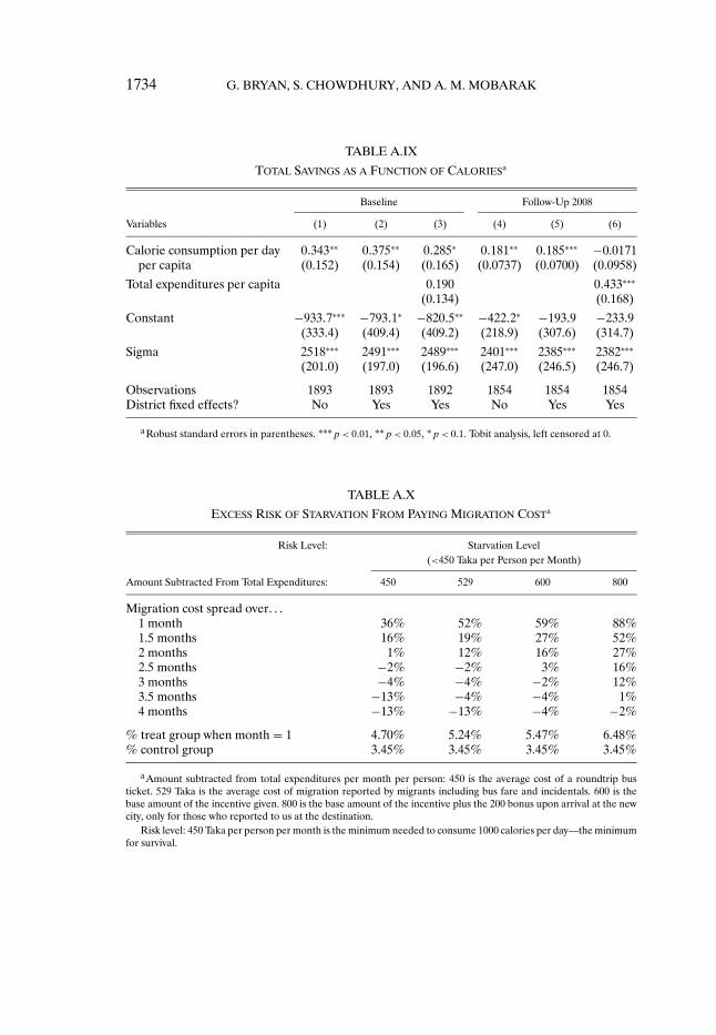
1734 G. BRYAN, S. CHOWDHURY, AND A. M. MOBARAK
TABLE A.IX
TOTAL SAVINGS AS A FUNCTION OF CALORIESa
Baseline Follow-Up 2008
Variables (1) (2) (3) (4) (5) (6)
Calorie consumption per day 0�343∗∗ 0�375∗∗ 0�285∗ 0�181∗∗ 0�185∗∗∗ −0.0171per capita (0.152) (0.154) (0.165) (0.0737) (0.0700) (0.0958)
Total expenditures per capita 0.190 0�433∗∗∗
(0.134) (0.168)
Constant −933�7∗∗∗ −793�1∗ −820�5∗∗ −422�2∗ −193.9 −233.9(333.4) (409.4) (409.2) (218.9) (307.6) (314.7)
Sigma 2518∗∗∗ 2491∗∗∗ 2489∗∗∗ 2401∗∗∗ 2385∗∗∗ 2382∗∗∗
(201.0) (197.0) (196.6) (247.0) (246.5) (246.7)
Observations 1893 1893 1892 1854 1854 1854District fixed effects? No Yes Yes No Yes Yes
aRobust standard errors in parentheses. ∗∗∗p< 0�01, ∗∗p< 0�05, ∗p< 0�1. Tobit analysis, left censored at 0.
TABLE A.X
EXCESS RISK OF STARVATION FROM PAYING MIGRATION COSTa
Risk Level: Starvation Level(<450 Taka per Person per Month)
Amount Subtracted From Total Expenditures: 450 529 600 800
Migration cost spread over� � �1 month 36% 52% 59% 88%1.5 months 16% 19% 27% 52%2 months 1% 12% 16% 27%2.5 months −2% −2% 3% 16%3 months −4% −4% −2% 12%3.5 months −13% −4% −4% 1%4 months −13% −13% −4% −2%
% treat group when month = 1 4.70% 5.24% 5.47% 6.48%% control group 3.45% 3.45% 3.45% 3.45%
aAmount subtracted from total expenditures per month per person: 450 is the average cost of a roundtrip busticket. 529 Taka is the average cost of migration reported by migrants including bus fare and incidentals. 600 is thebase amount of the incentive given. 800 is the base amount of the incentive plus the 200 bonus upon arrival at the newcity, only for those who reported to us at the destination.
Risk level: 450 Taka per person per month is the minimum needed to consume 1000 calories per day—the minimumfor survival.

UNDERINVESTMENT IN A PROFITABLE TECHNOLOGY 1735
TABLE A.XI
GOING BACK TO THE SAME EMPLOYER IN 2011a
Full Sample
Incentivized in 2008 0�047∗
(0.027)
Constant 0�266∗∗∗
(0.020)
Observations 2771R-squared 0.003
aRobust standard errors in parentheses. ∗∗∗p < 0�01, ∗∗p <0�05, ∗p< 0�1. The dependent variable is equal to 1 if a respondentreports going to the same employer in 2011 as before; 0 otherwise.
TABLE A.XIIa
PROPORTION OF 2011 MIGRANTS WHO FIRST MET EMPLOYER BEFORE OR AFTER MIGRATIONINCENTIVE (2006–2007 VS. 2008–2009), INCENTIVIZED IN 2008 ONLY
[MIGRANT ONLY SAMPLE; NON-EXPERIMENTAL]a
2007 2008 Diff. p-Value Observations
First met employer 0.42 0.58 −0.17 0.0941 103in 2007 vs. 2008 (0.05) (0.05)
2006–2007 2008–2009 Diff. p-Value Observations
First met employer 0.43 0.57 −0.13 0.0567 201in 2006–2007 vs. 2008–2009 (0.04) (0.04)
aStandard errors in parentheses. This table shows the proportion of migrants who were incentivized in 2008, whore-migrated in 2011, returned to the same place and met their employer between 2006 and 2009.
TABLE A.XIIb
PROPORTION OF 2011 MIGRANTS WHO FIRST MET EMPLOYER BEFORE OR AFTERINCENTIVIZATION (2006–2007 VS. 2008–2009), FULL SAMPLE
[MIGRANT ONLY SAMPLE; NON-EXPERIMENTAL]a
Not Incentivized Incentivized Diff. p-Value Observations
First met employer in 2008 0.50 0.58 −0.08 0.2589 189(rather than 2007) (0.05) (0.05)
Not Incentivized Incentivized Diff. p-Value Observations
First met employer in 2006–2007 0.54 0.57 −0.03 0.5672 363rather than 2008–2009 (0.04) (0.04)
aStandard errors in parentheses. This table shows the proportion of all migrants from 2008 who re-migrated in2011, returned to the same place and met their employer between 2006 and 2009.

1736G
.BR
YA
N,S.C
HO
WD
HU
RY
,AN
DA
.M.M
OB
AR
AK
TABLE A.XIIIa
DESTINATION CHOICES OF RE-MIGRANTSa
Panel A. Dep. Var.: Migrated in 2009 to: Dhaka Bogra Tangail Munshigonj
OLS IV OLS IV OLS IV OLS IV
Migrated in 2008 to 0�413∗∗∗ 0�679∗Dhaka (0.052) (0.348)
Migrated in 2008 to 0�333∗∗∗ 0.051Bogra (0.061) (0.177)
Migrated in 2008 to 0�463∗∗∗ 0.108Tangail (0.057) (0.184)
Migrated in 2008 to 0�233∗∗∗ 0�304∗Munshigonj (0.050) (0.185)
Constant 0�317∗∗∗ 0.213 −0.014 −0.002 0.027 0.073 0.059 0.038(0.068) (0.148) (0.012) (0.008) (0.050) (0.054) (0.037) (0.060)
Observations 589 589 589 589 589 589 589 589R-squared 0.195 0.132 0.205 0.032 0.305 0.081 0.155 0.0851st F-test 1.139 4.338 2.116 0.9801st p-value 0.345 0.000166 0.0412 0.4561st partial R2 0.0119 0.0561 0.0616 0.0217Hansen J0 4.272 7.142 8.882 3.920
(Continues)
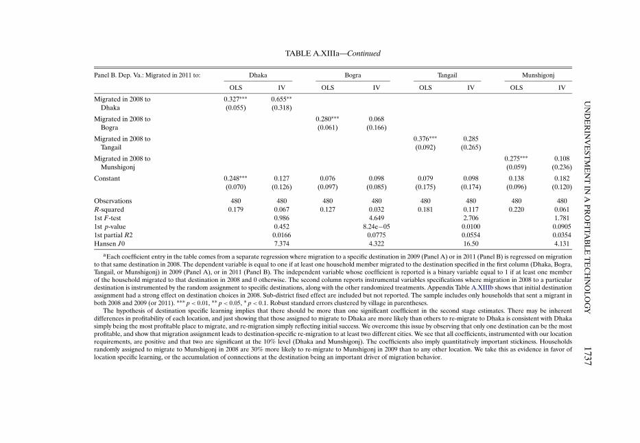
UN
DE
RIN
VE
STM
EN
TIN
APR
OF
ITAB
LE
TE
CH
NO
LO
GY
1737TABLE A.XIIIa—Continued
Panel B. Dep. Va.: Migrated in 2011 to: Dhaka Bogra Tangail Munshigonj
OLS IV OLS IV OLS IV OLS IV
Migrated in 2008 to 0�327∗∗∗ 0�655∗∗Dhaka (0.055) (0.318)
Migrated in 2008 to 0�280∗∗∗ 0.068Bogra (0.061) (0.166)
Migrated in 2008 to 0�376∗∗∗ 0.285Tangail (0.092) (0.265)
Migrated in 2008 to 0�275∗∗∗ 0.108Munshigonj (0.059) (0.236)
Constant 0�248∗∗∗ 0.127 0.076 0.098 0.079 0.098 0.138 0.182(0.070) (0.126) (0.097) (0.085) (0.175) (0.174) (0.096) (0.120)
Observations 480 480 480 480 480 480 480 480R-squared 0.179 0.067 0.127 0.032 0.181 0.117 0.220 0.0611st F-test 0.986 4.649 2.706 1.7811st p-value 0.452 8.24e−05 0.0100 0.09051st partial R2 0.0166 0.0775 0.0554 0.0354Hansen J0 7.374 4.322 16.50 4.131
aEach coefficient entry in the table comes from a separate regression where migration to a specific destination in 2009 (Panel A) or in 2011 (Panel B) is regressed on migrationto that same destination in 2008. The dependent variable is equal to one if at least one household member migrated to the destination specified in the first column (Dhaka, Bogra,Tangail, or Munshigonj) in 2009 (Panel A), or in 2011 (Panel B). The independent variable whose coefficient is reported is a binary variable equal to 1 if at least one memberof the household migrated to that destination in 2008 and 0 otherwise. The second column reports instrumental variables specifications where migration in 2008 to a particulardestination is instrumented by the random assignment to specific destinations, along with the other randomized treatments. Appendix Table A.XIIIb shows that initial destinationassignment had a strong effect on destination choices in 2008. Sub-district fixed effect are included but not reported. The sample includes only households that sent a migrant inboth 2008 and 2009 (or 2011). ∗∗∗p< 0�01, ∗∗p< 0�05, ∗p< 0�1. Robust standard errors clustered by village in parentheses.
The hypothesis of destination specific learning implies that there should be more than one significant coefficient in the second stage estimates. There may be inherentdifferences in profitability of each location, and just showing that those assigned to migrate to Dhaka are more likely than others to re-migrate to Dhaka is consistent with Dhakasimply being the most profitable place to migrate, and re-migration simply reflecting initial success. We overcome this issue by observing that only one destination can be the mostprofitable, and show that migration assignment leads to destination-specific re-migration to at least two different cities. We see that all coefficients, instrumented with our locationrequirements, are positive and that two are significant at the 10% level (Dhaka and Munshigonj). The coefficients also imply quantitatively important stickiness. Householdsrandomly assigned to migrate to Munshigonj in 2008 are 30% more likely to re-migrate to Munshigonj in 2009 than to any other location. We take this as evidence in favor oflocation specific learning, or the accumulation of connections at the destination being an important driver of migration behavior.

1738 G. BRYAN, S. CHOWDHURY, AND A. M. MOBARAK
TABLE A.XIIIb
FIRST STAGE OF INSTRUMENTAL VARIABLES REGRESSION FOR DESTINATIONCHOICES FOR 2009 MIGRANTSa
Dep. Var.: Migrated in 2008 to: Dhaka Bogra Tangail Munshigonj
Cash −0.032 0�125∗∗ −0.052 0.010(0.088) (0.051) (0.075) (0.083)
Credit 0.035 0�085∗ 0.017 −0.056(0.088) (0.048) (0.077) (0.083)
Info 0.009 0.052 0.016 0.019(0.102) (0.049) (0.088) (0.094)
Group formation—self-formed −0.045 0.022 −0.022 −0.011(0.046) (0.053) (0.054) (0.051)
Group formation—assigned −0.001 0.053 −0.041 0.008(0.058) (0.057) (0.051) (0.049)
Group formation—two people −0.048 −0.018 0.059 0.054(0.050) (0.052) (0.066) (0.072)
Destination assigned −0.020 −0�059∗ −0�078∗ −0.007(0.044) (0.033) (0.045) (0.037)
Assigned to Dhaka 0.054(0.068)
Assigned to Bogra 0�234∗∗∗
(0.066)
Assigned to Tangail 0�305∗∗∗
(0.084)
Assigned to Munshigonj 0�163∗∗
(0.080)
Constant 0�427∗∗∗ −0�075∗ 0�142∗ 0.295(0.148) (0.043) (0.072) (0.187)
Observations 589 589 589 589F-statistic 1.139 4.338 2.116 0.980prob >F 0.345 0.000166 0.0412 0.456Partial R2 0.0119 0.0561 0.0616 0.0217Hansen J statistic 4.272 7.142 8.882 3.920R-squared 0.092 0.103 0.197 0.097
a ∗∗∗p< 0�01, ∗∗p< 0�05, ∗p< 0�1. Robust standard errors in parentheses.

UNDERINVESTMENT IN A PROFITABLE TECHNOLOGY 1739
TABLE A.XIV
EXPECTATIONS ABOUT FINDING A JOB AND EARNINGS(NON-EXPERIMENTAL: ASKED OF 2008 MIGRANTS)a
Incentivized Not Incentivized Diff.
Expectations About Finding a JobToo optimistic (job search took more time than expected) 0.18 0.14 0.05
(0.01) (0.02) (0.03)
Too pessimistic (job search took less time than expected) 0.24 0.27 −0.03(0.02) (0.03) (0.03)
As expected 0.58 0.59 −0.01(0.02) (0.03) (0.04)
Expectations About Earnings at the DestinationToo optimistic (earned less than expected) 0.42 0.39 0.03
(0.02) (0.03) (0.04)
Too pessimistic (earned more than expected) 0.26 0.27 0.00(0.02) (0.03) (0.03)
As expected 0.32 0.34 −0.02(0.02) (0.03) (0.04)
Expectations About the Severity of MongaMonga (1–100 scale) 78.71 77.05 1.04
(0.58) (0.89) (1.66)
aStandard errors in parentheses.

1740 G. BRYAN, S. CHOWDHURY, AND A. M. MOBARAK
FIGURE A.1.—Distribution of consumption per person per month by baseline consumptiondecile.

UNDERINVESTMENT IN A PROFITABLE TECHNOLOGY 1741
FIGURE A.2.—Distribution of calories per person per day in 2008.

1742 G. BRYAN, S. CHOWDHURY, AND A. M. MOBARAK
FIGURE A.3.—Value functions of migrating and non-migrating households.
FIGURE A.4.—Policy functions (consumption as a function of cash on hand) for householdsbad at migrating and households restricted from migrating.

UNDERINVESTMENT IN A PROFITABLE TECHNOLOGY 1743
FIGURE A.5.—Simulated cash on hand and consumptions for varying levels of wealth.

1744 G. BRYAN, S. CHOWDHURY, AND A. M. MOBARAK
REFERENCES
ADAMS, R. H. (1998): “Remittances, Investment, and Rural Asset Accumulation in Pakistan,”Economic Development and Cultural Change, 47 (1), 155–173. [1672]
AKEE, R. (2010): “Who Leaves? Deciphering Immigrant Self-Selection From a DevelopingCountry,” Economic Development and Cultural Change, 58 (2), 323–344. [1672]
ANH, D. N. (2003): “Migration and Poverty in Asia: With Reference to Bangladesh, China, thePhilippines and Viet Nam,” in Ad hoc Expert Group Meeting on Migration and Development,Organised by the Economic and Social Commission for Asia and the Pacific, Bangkok, 27–29August. [1718]
ARDINGTON, C., A. CASE, AND V. HOSEGOOD (2009): “Labor Supply Responses to Large SocialTransfers: Longitudinal Evidence From South Africa,” American Economic Journal: AppliedEconomics, 1 (1), 22–48. [1673,1718]
ASHRAF, N., D. AYCINENA, C. A. MARTINEZ, AND D. YANG (2014): “Remittances and the Prob-lem of Control: A Field Experiment Among Migrants From El Salvador,” Review of Economicsand Statistics (forthcoming). [1672]
AYCINENA, D., C. A. MARTINEZ, AND D. YANG (2010): “The Impact of Remittance Fees onRemittance Flows: Evidence From a Field Experiment Among Salvadoran Migrants,” Report,University of Michigan. [1672]
BANDIERA, O., I. BARANKAY, AND I. RASUL (2011): “Field Experiments With Firms,” Journal ofEconomic Perspectives, 25 (3), 63–82. [1718]
BANERJEE, A. (2004): “The Two Poverties,” in Insurance Against Poverty, ed. by S. Dercon. Ox-ford: Oxford University Press, 59–75. [1673,1695]
BANERJEE, A., AND E. DUFLO (2007): “The Economic Lives of the Poor,” Journal of EconomicPerspectives, 21 (1), 141–167. [1677]
BANERJEE, A., AND S. MULLAINATHAN (2010): “The Shape of Temptation: Implications for theEconomic Lives of the Poor,” Working Paper. [1717]
BANERJEE, A., AND A. F. NEWMAN (1991): “Risk-Bearing and the Theory of Income Distribu-tion,” Review of Economic Studies, 58 (2), 211–235. [1673]
BANGLADESH BUREAU OF STATISTICS (2011): “Monthly Statistical Bulletins,” available at http://www.bbs.gov.bd/home.aspx. [1677]
BARHAM, B., AND S. BOUCHER (1998): “Migration, Remittances, and Inequality: Estimating theNet Effects of Migration on Income Distribution,” Journal of Development Economics, 55 (2),307–331. [1672]
BASU, K., AND M. WONG (2012): “Evaluating Seasonal Food Security Programs in East Indone-sia,” Working Paper 51219, MPRA. Available at http://mpra.ub.uni-muenchen.de/51219. Jour-nal of Development Economics (forthcoming). [1672]
BEEGLE, K., J. DE WEERDT, AND S. DERCON (2011): “Migration and Economic Mobility inTanzania: Evidence From a Tracking Survey,” Review of Economics and Statistics, 93 (3),1010–1033. [1672,1689]
BENYISHAY, A., AND A. M. MOBARAK (2013): “Social Learning and Communication,” Unpub-lished Manuscript, Yale University. [1674]
BORJAS, G. (2003): “The Labor Demand Curve Is Downward Sloping: Reexamining the Impactof Immigration on the Labor Market,” Quarterly Journal of Economics, 118 (4), 1335–1374.[1718]
BORJAS, G., AND L. KATZ (2007): “The Evolution of the Mexican-Born Workforce in the UnitedStates,” in Mexican Immigration to the United States, ed. by G. Borjas. Chicago: University ofChicago Press, 13–56. [1718]
BROWN, R., AND G. LEEVES (2007): “Impacts of International Migration and Remittances onSource Country Household Incomes in Small Island States: Fiji and Tonga,” Discussion Pa-per 347, School of Economics, University of Queensland. [1672]
BRUNE, L., X. GINE, J. GOLDBERG, AND D. YANG (2011): “Commitments to Save: A Field Ex-periment in Rural Malawi,” Policy Research Working Paper 5748, World Bank. [1672]

UNDERINVESTMENT IN A PROFITABLE TECHNOLOGY 1745
BRYAN, G., S. CHOWDHURY, AND A. MOBARAK (2014): “Supplement to ‘Underinvestment in aProfitable Technology: The Case of Seasonal Migration in Bangladesh’,” Econometrica Supple-mental Material, 82, http://www.econometricsociety.org/ecta/supmat/10489_miscellaneous.pdf;http://www.econometricsociety.org/ecta/supmat/10489_data_and_programs.zip. [1712]
BUERA, F. J. (2009): “A Dynamic Model of Entrepreneurship With Borrowing Constraints: The-ory and Evidence,” Annals of Finance, 5, 443–464. [1695,1721]
CARD, D. (2009): “Immigration and Inequality,” American Economic Review, 99 (2), 1–21. [1718]CARROLL, C. D. (2001): “A Theory of the Consumption Function, With and Without Liquidity
Constraints,” Journal of Economic Perspectives, 15 (3), 23–45. [1697]CASELLI, F. (2005): “Accounting for Cross-Country Income Differences,” in Handbook of Eco-
nomic Growth, Vol. 1A, ed. by P. Aghion and S. Durlauf. Amsterdam: Elsevier, 679–741. [1673]CHAUDHURI, S., AND C. PAXSON (2002): “Smoothing Consumption Under Income Seasonal-
ity: Buffer Stocks vs. Credit Markets,” Discussion Paper 0102-54, Department of Economics,Columbia University. Available at http://hdl.handle.net/10022/AC:P:363. [1672]
CHETTY, R., AND A. SZEIDL (2007): “Consumption Commitments and Risk Preferences,” Quar-terly Journal of Economics, 122 (2), 831–877. [1715]
CHIN, A., L. KARKOVIATA, AND N. WICOX (2010): “Impact of Bank Accounts on Migrant Savingsand Remittances: Evidence From a Field Experiment,” Report. [1672]
CLARKE, D. J. (2011): “A Theory of Rational Demand for Index Insurance,” Discussion Paper572, Department of Economics, University of Oxford. Available at http://www.economics.ox.ac.uk/department-of-economics-discussion-paper-series/a-theory-of-rational-demand-for-index-insurance. [1700]
CLEMENS, M. (2010): “The Roots of Global Wage Gaps: Evidence From Randomized Processingof U.S. Visas,” Working Paper 212, Center for Global Development. [1672]
(2011): “Economics and Emigration: Trillion-Dollar Bills on the Sidewalk?” Journal ofEconomic Perspectives, 25 (3), 83–106. [1717]
CLEMENS, M., C. E. MONTENEGRO, AND L. PRITCHETT (2008): “The Place Premium: Wage Dif-ferences for Identical Workers Across the U.S. Border,” Working Paper 148, Center for GlobalDevelopment. [1717]
DE MEL, S., D. MCKENZIE, AND C. WOODRUFF (2008): “Returns to Capital in Microenterprises:Results From a Randomized Experiment,” Quarterly Journal of Economics, 123 (4), 1329–1372.[1718]
DEATON, A. (1991): “Savings and Liquidity Constraints,” Econometrica, 59 (5), 1221–1248. [1693,1694,1697,1721]
(1997): The Analysis of Household Surveys: A Microeconometric Approach to DevelopmentPolicy. Baltimore: Johns Hopkins University Press for the World Bank. [1685,1697]
DERCON, S., AND L. CHRISTIAENSEN (2011): “Consumption Risk, Technology Adoption andPoverty Traps: Evidence From Ethiopia,” Journal of Development Economics, 96 (2), 159–173.[1674]
DERCON, S., AND P. KRISHNAN (2000): “Vulnerability, Seasonality and Poverty in Ethiopia,” Jour-nal of Development Studies, 36 (6), 25–53. [1671]
DOSTIE, B., S. HAGGBLADE, AND J. RANDRIAMAMONJY (2002): “Seasonal Poverty in Madagas-car: Magnitude and Solutions,” Food Policy, 27 (5/6), 493–518. [1672]
DUFLO, E., M. KREMER, AND J. ROBINSON (2011): “Nudging Farmers to Use Fertilizer: Theoryand Experimental Evidence From Kenya,” American Economic Review, 101 (6), 2350–2390.[1717,1718]
DUPAS, P. (2014): “Short-Run Subsidies and Long-Run Adoption of New Health Products: Evi-dence From a Field Experiment,” Econometrica, 82 (1), 197–228. [1674]
DUPAS, P., AND J. ROBINSON (2013): “Why Don’t the Poor Save More? Evidence From HealthSavings Experiments,” American Economic Review, 103 (4), 1138–1171. [1697,1716]
EECKHOUDT, L., C. GOLLIER, AND H. SCHLESINGER (1996): “Changes in Background Risk andRisk Taking Behavior,” Econometrica, 64 (3), 683–689. [1695]

1746 G. BRYAN, S. CHOWDHURY, AND A. M. MOBARAK
EVENSON, R. E., AND D. GOLLIN (2003): “Assessing the Impact of the Green Revolution, 1960to 2000,” Science, 300, 758–762. [1673]
FAFCHAMPS, M., D. MCKENZIE, S. R. QUINN, AND C. WOODRUFF (2011): “When Is CapitalEnough to Get Female Microenterprises Growing? Evidence From a Randomized Experimentin Ghana,” Working Paper 17207, NBER. [1718]
FISCHER, G. (2013): “Contract Structure, Risk Sharing and Investment Choice,” Econometrica,81 (3), 883–939. [1674]
FOSTER, A., AND M. R. ROSENZWEIG (2010): “Microeconomics of Technology Adoption,” An-nual Review of Economics, 2 (1), 395–424. [1685]
(2011): “Are Indian Farms Too Small? Mechanization, Agency Costs and Farm Effi-ciency,” Working Paper. [1674]
GIBSON, J., AND D. MCKENZIE (2010): “The Development Impact of a Best Practice SeasonalWorker Policy,” Working Paper 286, BREAD. Available at https://ipl.econ.duke.edu/bread/working/286. [1672,1717]
GIBSON, J., D. MCKENZIE, AND S. STILLMAN (2013): “Accounting for Selectivity and Duration-Dependent Heterogeneity When Estimating the Impact of Emigration on Incomes and Povertyin Sending Areas,” Economic Development and Cultural Change, 61 (2), 247–280. [1672]
GINE, X., AND D. YANG (2009): “Insurance, Credit, and Technology Adoption: Field Experimen-tal Evidence From Malawi,” Journal of Development Economics, 89 (1), 1–11. [1723]
GOLLIER, C. (2004): The Economics of Risk and Time. Cambridge: MIT Press. [1697]GOLLIN, D., D. LAGAKOS, AND M. E. WAUGH (2011): “The Agricultural Productivity Gap in
Developing Countries,” Working Paper 11-14, Department of Economics, Leonard N. SternSchool of Business, New York University. Available at https://files.nyu.edu/mw134/public/uploads/56836/apg.pdf. [1673]
GOLLIN, D., S. PARENTE, AND R. ROGERSON (2002): “The Role of Agriculture in Development,”American Economic Review: Papers and Proceedings, 92 (2), 160–164. [1673]
GOVERNMENT OF PEOPLE’S REPUBLIC OF BANGLADESH (2005): Bangladesh: Poverty Reduc-tion Strategy Paper: Unlocking the Potential, National Strategy for Accelerated Poverty Reduction.Washington, DC: International Monetary Fund. [1718]
GROGGER, J., AND G. H. HANSON (2011): “Income Maximization and the Selection and Sortingof International Migrants,” Journal of Development Economics, 95 (1), 42–57. [1672]
HANSON, G. H. (2009): “The Economic Consequences of the International Migration of Labor,”Annual Review of Economics, 1, 179–208. [1717]
HATTON, T., AND J. WILLIAMSON (1998): The Age of Mass Migration: An Economic Analysis. NewYork: Oxford University Press. [1673,1718]
HAUSMANN, R., AND D. RODRIK (2003): “Economic Development as Self-Discovery,” Journal ofDevelopment Economics, 72 (2), 603–633. [1674]
HOLT, C. A., AND S. K. LAURY (2002): “Risk Aversion and Incentive Effects,” American EconomicReview, 92 (5), 1644–1655. [1715]
JAIN, T., AND A. SOOD (2012): “How Does Relationship Based Governance Accomodate NewEntrants? Evidence From the Cycle Rickshaw Rental Market,” Working Paper 1586226, SSRN.Available at http://ssrn.com/abstract=1586226. [1704]
JAKIELA, P., AND O. OZIER (2012): “Does Africa Need a Rotten Kin Theorem? ExperimentalEvidence From Village Economies,” Working Paper. [1716]
JALAN, J., AND M. RAVALLION (2001): “Behavioral Responses to Risk in Rural China,” Journalof Development Economics, 66 (1), 23–49. [1672,1719]
JENSEN, R. T., AND N. H. MILLER (2008): “Giffen Behavior and Subsistence Consumption,”American Economic Review, 98 (4), 1553–1577. [1707]
KABOSKI, J. P., AND R. M. TOWNSEND (2011): “A Structural Evaluation of a Large-Scale Quasi-Experimental Microfinance Initiative,” Econometrica, 79 (5), 1357–1406. [1674]
KANBUR, R. (1979): “Of Risk Taking and the Personal Distribution of Income,” Journal of Politi-cal Economy, 87 (4), 769–797. [1673]

UNDERINVESTMENT IN A PROFITABLE TECHNOLOGY 1747
KANDEL, S., AND R. F. STAMBAUGH (1991): “Asset Returns and Intertemporal Preferences,” Jour-nal of Monetary Economics, 27 (1), 39–71. [1715]
KHANDKER, S. R. (2012): “Seasonality of Income and Poverty in Bangladesh,” Journal of Devel-opment Economics, 97 (2), 244–256. [1677]
KHANDKER, S. R., AND W. MAHMUD (2012): Seasonal Hunger and Public Policies: Evidence FromNorthwest Bangladesh. Washington, DC: The World Bank. [1672,1676]
KHANDKER, S. R., M. A. KHALEQUE, AND H. SAMAD (2011): “Can Social Safety Nets Allevi-ate Seasonal Deprivation? Evidence From Northwest Bangladesh,” Policy Research WorkingPaper 5865, World Bank. [1683,1718]
KIHLSTROM, R., AND J. LAFFONT (1979): “A General Equilibrium Entrepreneurial Theory ofFirm Formation Based on Risk Aversion,” Journal of Political Economy, 87 (4), 719–748. [1673]
KIMBALL, M. S. (1990): “Precautionary Saving in the Small and in the Large,” Econometrica, 58(1), 53–73. [1722]
KOSZEGI, B., AND M. RABIN (2006): “A Model of Reference-Dependent Preferences,” QuarterlyJournal of Economics, 121 (4), 1133–1165. [1717]
LAIBSON, D. (1997): “Golden Eggs and Hyperbolic Discounting,” Quarterly Journal of Economics,112 (2), 443–478. [1717]
LEWIS, W. A. (1955): The Theory of Economic Growth. London: Allen & Unwin. [1717]MACOURS, K., AND R. VAKIS (2010): “Seasonal Migration and Early Childhood Development,”
World Development, 38 (6), 857–869. [1672]MARTINEZ, C. A., AND D. YANG (2005): “Remittances and Poverty in Migrants’ Home Areas:
Evidence From the Philippines,” in International Migration, Remittances, and the Brain Drain,ed. by C. Ozden and M. Schiff. Washington, DC: The World Bank. [1672]
MCKENZIE, D. (2012): “Learning About Migration Through Experiments,” Discussion Pa-per 07/12, CReAM. Available at http://www.cream-migration.org/publ_uploads/CDP_07_12.pdf. [1672]
MCKENZIE, D., AND H. RAPOPORT (2007): “Network Effects and the Dynamics of Migrationand Inequality: Theory and Evidence From Mexico,” Journal of Development Economics, 84(1), 1–24. [1672]
MCKENZIE, D., AND D. YANG (2010): “Experimental Approaches in Migration Studies,” Discus-sion Paper 5125, Institute for the Study of Labor. [1672]
MCKENZIE, D., J. GIBSON, AND S. STILLMAN (2007): “A Land of Milk and Honey With StreetsPaved With Gold: Do Emigrants Have Over-Optimistic Expectations About Incomes Abroad,”Policy Research Working Paper 4141, World Bank. [1694,1716]
MCMILLAN, M., AND D. RODRIK (2011): “Globalization, Structural Change and ProductivityGrowth,” Working Paper 17143, NBER. [1673]
MEREDITH, J., J. ROBINSON, S. WALKER, AND B. WYDICK (2013): “Keeping the Doctor Away:Experimental Evidence on Investment in Preventative Health Products,” Journal of Develop-ment Economics, 105, 196–210. Available at http://people.ucsc.edu/~jmrtwo/HealthProducts.pdf. [1674]
MOBARAK, A. M., AND M. R. ROSENZWEIG (2013): “Informal Risk Sharing, Index Insurance,and Risk Taking in Developing Countries,” American Economic Review, 103 (3), 375–380.[1674]
MOBARAK, A. M., P. DWIVEDI, R. BAILIS, L. HILDEMANN, AND G. MILLER (2012): “Low De-mand for Nontraditional Cookstove Technologies,” Proceedings of the National Academy of Sci-ences of the United States of America, 109 (27), 10815–10820. [1674]
MUNSHI, K. (2004): “Social Learning in a Heterogeneous Population: Technology Diffusion inthe Indian Green Revolution,” Journal of Development Economics, 73 (1), 185–213. [1674]
MUNSHI, K., AND M. R. ROSENZWEIG (2009): “Why Is Mobility in India so Low? Social Insur-ance, Inequality, and Growth,” Working Paper 14850, NBER. [1717]
OTTAVIANO, G. I., AND G. PERI (2012): “Rethinking the Effect of Immigration on Wages,” Jour-nal of the European Economic Association, 10 (1), 152–197. [1718]
1748 G. BRYAN, S. CHOWDHURY, AND A. M. MOBARAK
PAXSON, C. (1993): “Consumption and Income Seasonality in Thailand,” Journal of PoliticalEconomy, 101 (1), 39–72. [1672]
PAXSON, C. H. (1992): “Using Weather Variability to Estimate the Response of Savings to Tran-sitory Income in Thailand,” American Economic Review, 82 (1), 15–33. [1697]
PING, H. (2003): “China Migration Country Study,” paper presented in Regional Conference onMigration, Development and Pro-Poor Policy Choices in Asia, Organised by the BangladeshRefugee and Migratory Movements Research Unit/DFID, Dhaka, Bangladesh, 22–24 June,2003. [1718]
RAHMAN, H. Z. (1995): “Mora Kartik: Seasonal Deficits and the Vulnerability of the Rural Poor,”in Rethinking Rural Poverty: Bangladesh as a Case Study, ed. by H. Z. Rahman and M. Hossain.New Dehli, India: Sage Publications. [1676]
RESTUCCIA, D., D. T. YANG, AND X. ZHU (2008): “Agriculture and Aggregate Productivity:A Quantitative Cross-Country Analysis,” Journal of Monetary Economics, 55, 234–250. [1673]
RODRIK, D. (2007): “Be Our Guest,” New York Times, June 1. [1717]ROSENZWEIG, M. R. (2006): “Global Wage Differences and International Student Flows,” in
Brookings Trade Forum: Global Labor Markets?, ed. by S. M. Collins and C. Graham. Washing-ton, DC: Brookings Institution Press, 211–228. [1717]
ROSENZWEIG, M. R., AND K. I. WOLPIN (1993): “Credit Market Constraints, ConsumptionSmoothing, and the Accumulation of Durable Production Assets in Low-Income Countries:Investments in Bullocks in India,” Journal of Political Economy, 101 (2), 223–244. [1674]
SEN, A. (1981): Poverty and Famines: An Essay on Entitlement and Deprivation. Oxford: ClarendonPress. [1676]
SHONCHOY, A. (2010): “Seasonal Migration and the Effectiveness of Micro-Credit in theLean Period: Evidence From Bangladesh,” Discussion Paper 294, Institute of DevelopingEconomies. [1677]
SUBRAMANIAN, S., AND A. DEATON (1996): “The Demand for Food and Calories,” Journal ofPolitical Economy, 106 (5), 133–162. [1707]
SWIFT, J. (1989): “Why Are Rural People Vulnerable to Famine?” IDS Bulletin, 20 (2), 8–15.[1672]
UDRY, C., AND S. ANAGOL (2006): “The Return to Capital in Ghana,” American Economic Re-view, 96 (2), 388–393. [1718]
VERESHCHAGINA, G., AND H. A. HOPENHAYN (2009): “Risk Taking by Entrepreneurs,” Ameri-can Economic Review, 99 (5), 1808–1830. [1695,1721]
VOLLRATH, D. (2009): “How Important Are Dual Economy Effects for Aggregate Productivity?”Journal of Development Economics, 88 (2), 325–334. [1673]
YANG, D. (2008): “International Migration, Remittances and Household Investment: EvidenceFrom Philippine Migrants’ Exchange Rate Shocks,” The Economic Journal, 118 (528), 591–630.[1672]
ZUG, S. (2006): “Monga—Seasonal Food Insecurity in Bangladesh—Bringing the InformationTogether,” Journal of Social Studies, 111, 21–39. [1677]
London School of Economics, Houghton Street, London, WC2A 2AE, U.K.;[email protected],
School of Economics, The University of Sydney, C81 Biomedical Building,NSW 2006, Australia; [email protected],
andYale School of Management, 165 Whitney Avenue, P.O. Box 208200, New
Haven, CT 06520, U.S.A.; [email protected].
Manuscript received December, 2011; final revision received May, 2014.


