UNDER REVIEW AT IEEE TRANSACTIONS ON NETWORK...

UNDER REVIEW AT IEEE TRANSACTIONS ON NETWORK SCIENCE AND ENGINEERING 1

Comparing the Effects of Failures in Power Gridsunder the AC and DC Power Flow Models

Hale Cetinay, Saleh Soltan, Fernando A. Kuipers, Gil Zussman, and Piet Van Mieghem

Abstract—In this paper, we compare the effects of failures in power grids under the nonlinear AC and linearized DC power flowmodels. First, we numerically demonstrate that when there are no failures and the assumptions underlying the DC model are valid, theDC model approximates the AC model well in four considered test networks. Then, to evaluate the validity of the DC approximationupon failures, we numerically compare the effects of single line failures and the evolution of cascades under the AC and DC flowmodels using different metrics, such as yield (the ratio of the demand supplied at the end of the cascade to the initial demand). Wedemonstrate that the effects of a single line failure on the distribution of the flows on other lines are similar under the AC and DCmodels. However, the cascade simulations demonstrate that the assumptions underlying the DC model (e.g., ignoring power losses,reactive power flows, and voltage magnitude variations) can lead to inaccurate and overly optimistic cascade predictions. Particularly,in large networks the DC model tends to overestimate the yield. Hence, using the DC model for cascade prediction may result in amisrepresentation of the gravity of a cascade.

Index Terms—Power grids, AC versus DC, power flows, cascading failures, contingency analysis.

F

1 INTRODUCTION

POwer grids are vulnerable to external events, such asnatural disasters and cyber-attacks, as well as to internal

events, such as unexpected variability in load or generation,aging, and control device malfunction. The operation of apower grid is governed by the laws of physics [1], and theoutage of an element may result in a cascade of failuresand a blackout [2]. The recent blackouts in Turkey [3],India [4], U.S. and Canada [5] had devastating effects andas such motivated the study of power grid vulnerabilities tocascading failures (e.g., [2], [6], [7]).

Some of the recent work on cascading failures considersa topological perspective where, once a network elementfails, the neighboring elements also fail [8]. However, suchtopological models do not consider the actual power gridflow dynamics. More realistic cascading failures models usethe linearized direct current (DC) power flows [9], [10].However, DC power flows are based on a linearization ofthe nonlinear AC power flow dynamics. The induced lin-earization error can be small in large transmission grids [11]and high for some particular networks [12]. Motivated bythese observations, we study the effects of line failures andcascades under both the linearized DC model and a nonlinear ACmodel by performing simulations on four test networks.

First, we numerically evaluate the accuracy of the DCpower flow model when there are no failures. We demon-strate that when there are no failures, the assumptions un-derlying the DC power flow approximation (i.e., negligibleactive power losses, reasonably small phase angle differ-ences between the neighboring nodes, and small variations

• H. Cetinay, F. A. Kuipers, and P. Van Mieghem are with the facultyof Electrical Engineering, Mathematics and Computer Science, DelftUniversity of Technology, Delft, the Netherlands.E-mails: {H.Cetinay-Iyicil, F.A.Kuipers, P.F.A.VanMieghem}@tudelft.nl

• S. Soltan and G. Zussman are with the Elec. Eng. Dept., ColumbiaUniversity, New York, NY.E-mails: {saleh, gil}@ee.columbia.edu.

in the voltage magnitudes at nodes) are valid, and therefore,the DC power flow model approximates the AC power flowmodel relatively well in four considered test networks. Wefurther derive an analytical upper bound on the differencebetween the AC and the DC power flows based on the accu-racy of the DC approximation assumptions. The analyticalresults appear in the Appendix. These results quantify theaccuracy of the DC power flow model based on the accuracyof the approximation assumptions.

Then, we compare the effects of single line failures underthe AC and DC models. We numerically demonstrate thatthe DC model can also capture the effects of a single linefailure on the flow changes on other lines relatively closeto the AC model. For example, in nearly 80% and 98% ofthe observed values in the IEEE 30-bus network and Polishgrid, respectively, the magnitudes of the differences in theline flow change ratios (the ratio of the change in the flowon a line after a failure to its original flow value) and theline outage distribution factors (the ratio of the change inthe flow on a line after a failure to the flow value of thefailed line) are smaller than 0.05.

We then present an AC cascading failures model whichis based on the nonlinear power flow equations, and there-fore, is more realistic than the corresponding DC model.We empirically compare the AC and DC cascade modelsbased on robustness metrics that quantify the operationaland topological characteristics of the grid during a cascadefor all cascading failures initiated by a single and two linefailures. Our simulations demonstrate that the assumptionsunderlying the DC model (lossless network and ignoringreactive power flows and voltage variations) can lead toinaccurate and overly optimistic cascade predictions. Forexample, in the Polish grid, the difference between the yield(the ratio of the demand supplied at the end of the cascadeto the initial demand) under the AC and DC cascade modelsis more than 0.4, in 60% of the cascades initiated by two line


failures.Moreover, we empirically compare the AC and DC cas-

cades under different supply and demand balancing andline outage rules. Our simulation results show that thedifference between the cascade evolution under the AC andDC power flows depends on the balancing and line outagerules in power grids. In particular, the supply and demandbalancing rule which separates the excess supply or demandfrom the grid increases the difference between the AC andDC models the most.

The remainder of this paper is organized as follows.Section 2 reviews related work and Section 3 presents thepower flow equations. Section 4 presents the cascading fail-ures models. Section 5 presents the numerical comparison ofthe AC and DC flow models in four different test networksand Section 6 concludes the paper. Analytical results onthe difference between the AC and DC power flow modelsappear in the Appendix.

2 RELATED WORK

Contingency analysis and cascading failures in power gridshave been widely studied [2], [7], [13]–[15]. In this section,we briefly review some of the methods and their relation toour work. We note that there are several abstract models,borrowed from physics, for modeling cascades in powergrids (e.g., see [8], [16]–[18]). These models do not includethe power-flow dynamics in power grids and, hence, are outof scope of this paper.

The study of cascading failures in power grids was initi-ated in [19], [20] which used the linearized DC model and aprobabilistic outage rule for overloaded line failures. Similarcascade models have been used to study the properties ofthe cascades [10], [21]–[26], as well as to design controlschemes to mitigate the cascade [27], [28] and to detectvulnerable parts of the grid [7], [10], [29].

Due to their complexity, the AC power flow equationsare not as commonly used as the DC equations in studyingcascading failures in power grids. An AC model is utilizedin [7], [30], as well as in some (mostly commercial) softwaretools for modeling the evolution of the cascade [31]. Unfor-tunately, none of these tools is publicly available. Hence, forthe evaluation in this paper, we developed an AC cascadingfailures simulator, using the MATPOWER AC power flowsolver [32].

Previous work on determining the accuracy of the DCpower flow approximation includes [11], [12], [33]–[37].However, these works did not consider accuracy of the DCflows in predicting the evolution of a cascade. In [7], theDC and the AC cascading failures are compared when allthe buses (nodes) in the AC model are voltage controlled(PV) buses. To the best of our knowledge, this paper is the firstto compare the evolution of cascades in power grids under theDC and AC power flows in detail and for many of the publiclyavailable power grid networks [32], [38].

3 POWER FLOW EQUATIONS

In this section, we provide details on the AC and DC powerflow equations.

3.1 AC Power Flow Equations

A power grid with n nodes (buses) andm transmission linesconstitutes a complex network whose underlying topologycan be represented by an undirected graph G(N ,L), whereN denotes the set of nodes and L denotes the set of lines.The status of each node i is represented by its voltage Vi =|Vi|eiθi in which |Vi| is the voltage magnitude, θi is the phaseangle at node i, and i denotes the imaginary unit.

The goal of an AC power flow analysis is the compu-tation of the voltage magnitudes and phase angles at eachbus in steady-state conditions [39]. In the steady-state, whenthe admittance values to ground are negligible, the injectedapparent power Si at node i equals to

Si =n∑k=1k 6=i

Sik =n∑k=1k 6=i

Viy∗ik(V ∗i − V ∗k ) = Vi(YV)∗i (1)

where ∗ denotes the complex conjugation, V =[V1, . . . , Vn]T is the vector of node voltages, yik is theequivalent admittance of the lines from node i to k, and Y isthe n×n admittance matrix. The elements of the admittancematrix Y, which depend on the topology of the grid as wellas the admittance values of the lines, are defined as follows:

Yik =

∑i 6=k yik, if k = i

−yik, if k ∈ N(i)

0, if k /∈ N(i)

where N(i) denotes the direct neighbors of node i.Rewriting the admittance matrix as Y = G + iB where

G and B are real matrices, and using the definition of theapparent power Sik = P (AC)

ik + iQ(AC)ik in (1) leads to the

equations for the active power Pi and the reactive power Qiat each node i:

Pi =n∑k=1

|Vi||Vk|(Gik cos θik +Bik sin θik) (2)

Qi =n∑k=1

|Vi||Vk|(Gik sin θik −Bik cos θik) (3)

where θik = θi − θk.In the AC power flow analysis, each node i is categorized

into one of the following three types:

1) Slack node: The node for which the voltage is typi-cally 1.0. For convenience, it is indexed as node 1.The slack node compensates for network losses byemitting or absorbing power. The active power P1

and the reactive power Q1 need to be computed.2) Load node: The active power Pi and the reactive

power Qi at these nodes are known and the voltageVi needs to be computed.

3) Voltage controlled node: The active power Pi and thevoltage magnitude |Vi| at these nodes are knownand the reactive power Qi and the phase angle θineed to be computed.

3.2 DC Power Flow Equations

The AC power flow equations are nonlinear in the volt-ages. The DC power flow equation provide a linearized


approximation of the active power flows in the AC model.Linearization is possible under the following conditions[39]:

1) The difference between the voltage phase angles ofevery couple of neighboring nodes is small such thatsin θik ≈ θik and cos θik ≈ 1.

2) The active power losses are negligible, and there-fore, Y ≈ iB where B is the imaginary part of theadmittance matrix Y, calculated neglecting the lineresistances.

3) The variations in the voltage magnitudes |Vi| aresmall and, therefore, it is assumed that |Vi| = 1 ∀i.

Under these assumptions, given the active power Pi ateach node i, the phase angle of the nodes can be estimatedby θi using the DC power flow equations as follows:

Pi =n∑k=1k 6=i

P (DC)ik =

n∑k=1k 6=i

Bik(θi − θk) (4)

or in matrix form,P = −BΘ (5)

where P = [P1, P2, . . . , Pn]T, Θ = [θ1, . . . , θn]T. Notice thatthe vectors P and P are equal except in the slack node (firstentry) since in the DC power flows, the lines are lossless andtherefore P1 +

∑ni=2 Pi = 0.

By assuming that the phase angle at the slack node is 0,the phase angle of the nodes can be estimated uniquely bysolving (5) for the DC power flow.

In Section 5, we numerically compare the AC and DCpower flow models and demonstrate that when there areno failures, the DC power flows provide relatively accurateapproximation of the AC power flows on most of thenetwork lines. For more details of the DC power flow modeland its analytical accuracy based on the three assumptions,see the Appendix.

4 MODELING CASCADING FAILURES

An initial failure in power grids may result in subsequentfailures in other parts of the grid. These consecutive failuresfollowing an initial failure constitute a cascading failure. Inthis section, we follow [7], [9], [13], [26] and develop modelsfor cascading failures due to line failures in power grids.

When an initial set of lines fail, they are removed fromthe network. As a result of this removal, the network topol-ogy is changed, and the power grid can be divided into oneor more connected components. Following [9], we assumethat each connected component can operate autonomously.If there is no supply or no demand within a connectedcomponent Gk, the component becomes a dead component,and all the demand or supply nodes within the componentare put out of service. If there are both supply and demandnodes within a connected component Gk, the connectedcomponent remains an alive component, but the supply anddemand within the component should be balanced. We usetwo different supply and demand balancing rules [7], [9],[13]:

1) Shedding and curtailing: The amount of the powersupply or demand are reduced at all nodes by a

common factor. If the total active power supplyis more than the total active power demand in aconnected component Gk, the active power outputsof generators are curtailed. On the other hand, ifthe total active power supply is not sufficient toserve the total active power demand, load sheddingis performed to balance the supply and demandwithin Gk.

2) Separating and adjusting: Excess supply or demandnodes are separated from the grid. In this case, weassume that the dynamic response of the generators(demand nodes) are related to their sizes. Namely,the generators (demand nodes) with lower amountsof power output are faster to respond to the imbal-ances between supply and demand. Thus, withineach component Gk with excess supply (demand),the generators (demand nodes) are separated fromthe grid according their sizes from the smallest tolargest until the removal of one more generator(demand node) results in the shortage of supply(demand). Then, the active power output (demand)of the largest supply (demand) node is reduced inorder to balance supply and demand.

After supply and demand are balanced within each alivecomponent using the selected balancing rule, the powerflow equations are solved to compute new flows on thelines. The new set of line failures are then found in all alivecomponents. We use two different line outage rules [7], [13],[26]:

1) Deterministic: A line l fails when the power flowmagnitude on that line, denoted by |fl|, exceeds itscapacity cl.

2) Probabilistic: A line l fails with probability pl at eachstage of the cascade. We assume that each line lwith a flow capacity cl has also a nominal powerflow level ξl ∈ [0, cl], after which the line may failwith a certain probability (due to increase in linetemperature or sag levels). Under this model, theprobability pl is approximated as:

pl =

0, if |fl| < ξl|fl|−ξlcl−ξl , if ξl ≤ |fl| < cl

1, if |fl| ≥ cl.(6)

After finding the new set of line failures using theselected line outage rule, the cascade continues with theremoval of those lines. If there are no new line failures inany of the alive components, the cascade ends.

In this paper, we study three cascade processes:

I) Cascade with shedding and curtailing balancing ruleand deterministic line outage rule,

II) Cascade with separating and adjusting balancingrule and deterministic line outage rule,

III) Cascade with shedding and curtailing balancing ruleand probabilistic line outage rule.

In order to study the differences between the AC andDC models, we mostly focus on the cascade process I withshedding and curtailing balancing rule and deterministicline outage rule. In order to further capture the effects of


these processes on the differences obtained under the ACand DC models, in Subsection 5.5, we briefly compare thethree cascade processes.

In the following two Subsections, we provide the detailsof the cascade models under the AC and DC power flows.

4.1 AC Cascading Failures Model

In the cascade under the AC flow model, the flows are com-posed of active parts Pi in (2) and reactive parts Qi in (3).Hence, the apparent power Si in (1) is used to calculate theflows. In general, due to transmission line impedances, thevoltage at the sending node of a line is different than theone at the receiving node, resulting in different values of theapparent power flows at each side of the line. Hence, in thecascade under the AC model, we define the magnitude |fl|of flow on a line l = {i, k} as follows:

|fl| =|Sik|+ |Ski|

2. (7)

The difference, Sik − Ski, between the sent and receivedapparent flows on a line l represents the power loss overthat line. The sum of the losses over all the lines is the totalloss in the network. The total loss cannot be calculated inadvance and is only known after the power flow equationsin (1) are solved. Therefore, in the cascade under the ACflow, a part of the total supply in the network is reserved tosupply the network losses and denoted by the reserved lossfactor η.

The case of zero reserved loss factor, η = 0, means thatno reserve supply is allocated for network losses, whereasa large reserved loss factor η corresponds to a large re-serve supply for the network losses. Once the power flowequations are solved and the network losses are calculated,the difference between the allocated supply and the totaldemand with losses is compensated by the slack-node.Therefore, in the AC cascading failures model, the simula-tion is slack-node dependent, and for every alive componentwithout such a node, a slack-node must be assigned. Thedeveloped model chooses the slack-node as the voltagecontrolled node with the maximum power output in thatalive component.

The iterative process of solving the AC power flow equa-tions (2) and (3) may result in the absence of a solution or adivergence in iterations. In such cases, it is perceived that theconnected component cannot function at those operationalconditions, and supply and demand shedding is applied.The amount of active and reactive power demands, andactive power supply within that component are decreaseduntil either convergence is reached in the flow equationsor the component becomes a dead component with nodemand.

We numerically study the three cascade processes underthe AC flow model in Section 5.

4.2 DC Cascading Failures Model

In the cascade under the DC flow model, the magnitude |fl|of the flow on a line l = {i, k} is equal to the magnitude ofactive power flow in (4) on that line:

|fl| = |Pik| = |Pki|. (8)

Since the network is assumed to be lossless, the mag-nitude of the active power at the sending side of a lineis equal to the magnitude of active power at the receivingside, |Pik| = |Pki|, and the total supply is equal to the totaldemand. Therefore, the supply and demand balancing isperformed without a reserved loss factor η. Moreover, theno-loss assumption means that the flows in the network areslack-node independent.

Contrary to the AC flow equations (2) and (3), whichare nonlinear, the DC power flow equations (5) are linear,and a solution always exists for a connected network withbalanced supply and demand [40]. Hence, no supply ordemand shedding due to convergence issues is needed inthe DC model.

We numerically study the three cascade processes underthe DC flow model in Section 5.

5 NUMERICAL COMPARISON OF THE AC AND DCFLOW MODELS

This section presents the numerical comparison of the ACand DC power flow models. After providing the simulationssetup, we numerically evaluate the accuracy of the DCpower flow model when there are no failures. Then, wecompare the effects of single line failures, and the evolutionof the cascade process I initiated by single and doubleline failures under the AC and DC flow models. Next, wecompare the three cascade processes under the AC and DCflow models. Finally, we discuss the main lessons learnedfrom the simulations.

5.1 Simulations Setup

5.1.1 Metrics

We define metrics for evaluating the grid vulnerability(some of which were originally used in [10], [26], [40], [41]).To study the effects of a single line e failure on the flows onother lines we define:I Line flow change ratio (sl,e): the ratio ∆fl/fl of thechange ∆fl in the flow on a line l due to the failure at line eto its original flow value fl.I Line outage distribution factor (ml,e): the ratio ∆fl/feof the change ∆fl in the flow on a line l due to the failure atline e to the flow value fe of the failed line e.

Additionally, we define the following metrics to measureother dynamics of the system after a single line failure,which can only be captured under the AC power flowmodel due to the DC power flow assumptions 2 and 3 inSection 3.2:I Node voltage change (∆vi,e): the change in the voltagemagnitude at node i after the failure at line e.I Power loss change ratio (∆pµ,e): the ratio of the changein the active power output of the slack generator due to thefailure at line e to the initial loss.

We also define metrics to evaluate the cascade severity:I Node-loss ratio (NG): the ratio of the total number offailed nodes (i.e., nodes in dead components) at the end ofthe cascade to the total number of nodes.I Line-loss ratio (LG): the ratio of the total number of failedlines at the end of the cascade to the total number of lines.


I Yield (YG): the ratio of the demand supplied at the end ofthe cascade to the initial demand.

In addition to the previous metrics which capture theoverall effect of a cascading failure on a power grid, weidentify the frequently overloaded lines that may causecascading failures to persist. Hence, we defineI Line-vulnerability ratio (Rl): the total number of cas-cading failures in which line l is overloaded over the totalnumber of cascading failures simulations. Higher valuesof Rl indicate the vulnerability of the line l as a possiblebottleneck in the network.

5.1.2 Properties of the Networks used in SimulationsWe considered four realistic networks: the IEEE 30-bus, theIEEE 118-bus, and the IEEE 300-bus test systems [38], aswell as the Polish transmission grid [32]. The details of thesenetworks are as follows.I The IEEE 30-bus test system contains 30 nodes and 41lines with a total power demand of 189.2 MW.I The IEEE 118-bus test system contains 118 nodes and 186lines with a total power demand of 4242 MW.I The IEEE 300-bus test system contains 300 nodes and 411lines with a total power demand of 23,525.85 MW.I The Polish transmission grid, at summer 2008 morningpeak, contains 3120 nodes and 3693 lines with a total powerdemand of 21,181.5 MW.

In the IEEE test networks, maximum line flow capacitiesare not present. Following [9], the line flow capacities areestimated as cl = (1 + α) max{|fl|, f}, where α = 1 is theline tolerance, and f is the mean of the initial magnitude ofline flows.

In the Polish transmission grid data, emergency ratingsare used for the flow capacities of the network. In order toeliminate existing overloaded transmission lines at the basecase operation, the line flow capacities of such overloadedlines are changed to cl = (1 + α)|fl| where α = 1.

5.1.3 Power Flow SolverIn the simulations, we used MATPOWER [32] package inMATLAB for solving the AC and DC power flows.

5.2 No Failures CaseIn this section, we numerically evaluate the accuracy of theDC power flow model when there are no failures in fourtest networks. First, we check the validity of the assump-tions underlying the DC power flow approximation (asmentioned in Section 3.2). Then, we compute the absolutedifference between the AC and DC power flow models.

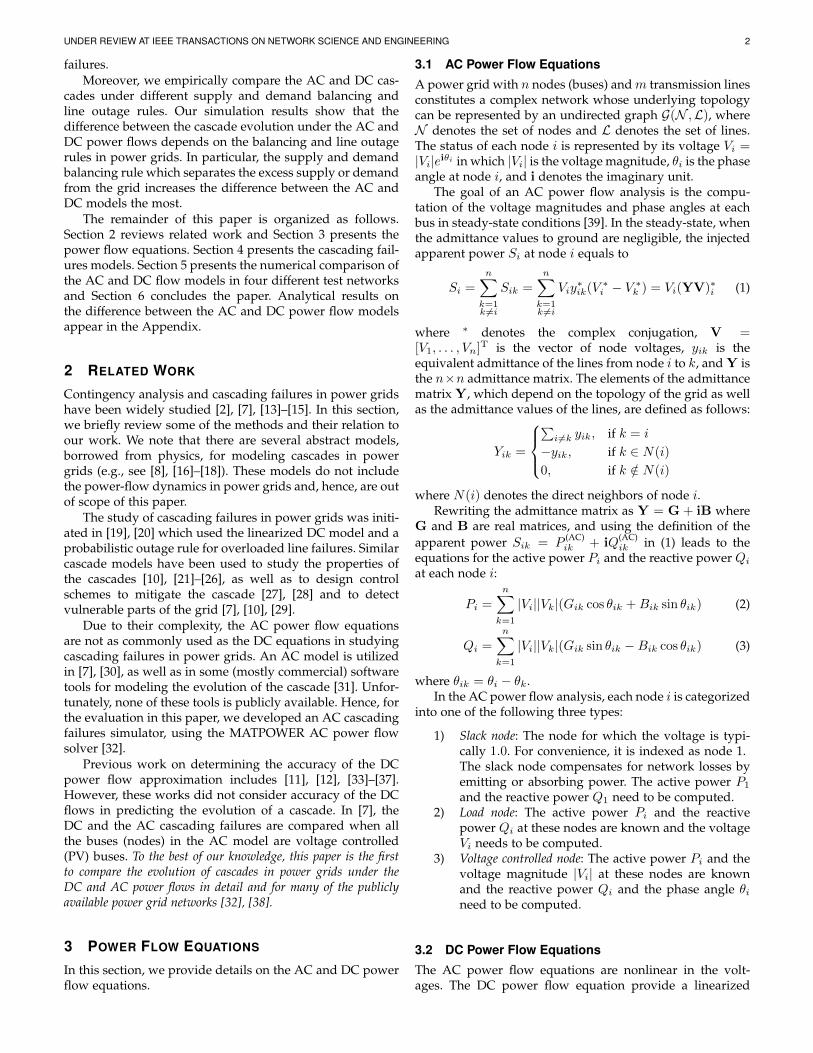
Fig. 1 shows the cumulative distribution functions(CDFs) of the absolute difference between the voltage phaseangle of neighboring nodes, the ratio of the real to imaginarypart of the admittance values, the deviation of the voltagemagnitudes from 1, and the absolute difference of the ACand DC active power flow.

In particular, Fig. 1a demonstrates that the differencebetween the voltage phase angles of neighboring nodes(condition 1) is less than 0.1 for 80% of the pairs in alltest networks. Fig. 1b shows that the imaginary part of theadmittance values are dominant (condition 2) in the testnetworks. Fig. 1c shows that the voltage magnitudes are

0 0.05 0.1 0.15 0.2 0.25x

0

0.2

0.4

0.6

0.8

1

FX(x

)

IEEE 30-busIEEE 118-busIEEE 300-busPolish Grid

(a) X := |θi − θj |

0 0.2 0.4 0.6 0.8 1x

0

0.2

0.4

0.6

0.8

1

FX(x

)


(b) X := |gij/bij |

0 0.05 0.1 0.15 0.2x

0

0.2

0.4

0.6

0.8

1

FX(x

)


(c) X := ||Vi| − 1|

0 0.2 0.4 0.6 0.8 1x

0

0.2

0.4

0.6

0.8

1

FX(x

)


(d) X := |P (AC)ij − P (DC)

ij |

Fig. 1. The validity of the assumptions underlying the DC power flowapproximation and the resulting difference between the AC and DCpower flow models: the CDFs of (a) the absolute difference betweenthe voltage phase angle of neighboring nodes, (b) the ratio of the real toimaginary part of the admittance values, (c) the deviation of the voltagemagnitudes from 1, and (d) the absolute difference of the AC and DCactive power flows.

close to 1.0 (condition 3) for all the nodes. Hence, as canbe seen in Fig. 1d, the differences between the AC and DCpower flows is less than 0.2 (p.u.) for nearly 80% of the lines.

Fig. 1 demonstrates that the assumptions underlyingthe DC power flow approximation are valid, and the DCpower flows approximate the AC power flows of most ofthe network lines relatively well when there are no failures.In the following subsections, we show that upon failures,however, the DC approximation may become inaccurate.Moreover, the small differences between the AC and DCpower flows in different cascade stages may lead to drasticdifferences at the end of the cascade.

5.3 Comparison of the Single Line Failure Effects

Single line failure and its consequent removal is the firststage and the triggering event of possible cascading failures.In this section, we perform empirical studies on singleline failures in four realistic networks. Since the line flowchange ratios sl,e for the lines with a low initial flow can beunreasonably high [10], these values are calculated only forthe lines whose initial flow is larger than the mean flow.Additionally, to capture the variations of the line outagedistribution factorsml,e and power loss change ratios ∆pµ,e,line failures that partition the network are not considered inthe set of failed lines.

Fig. 2 presents the CDFs of the differences in the line flowchange ratios and line outage distribution factors calculatedbased on the AC and DC flows. These results show that thedifferences decrease with the size of the network. In nearly80% of the observed values in the IEEE 30-bus network,the magnitudes of the differences in the line flow changeratios sl,e and the line outage distribution factors ml,e are


0 0.025 0.05 0.075 0.1x

0

0.1

0.2

0.3

0.4

0.5

0.6

0.7

0.8

0.9

1F

X(x

)


(a) X := |sACl,e − s

DCl,e|

0 0.025 0.05 0.075 0.1x

0

0.1

0.2

0.3

0.4

0.5

0.6

0.7

0.8

0.9

1

FX(x

)


(b) X := |mACl,e −m

DCl,e|

Fig. 2. The CDFs of the differences in the line flow change ratios and theline outage distribution factors based on the AC and DC flow models.

0 0.0025 0.005 0.0075 0.01x

0

0.1

0.2

0.3

0.4

0.5

0.6

0.7

0.8

0.9

1

FX(x

)


(a) X := |∆vACi,e|

0 0.05 0.1 0.15 0.2x

0

0.1

0.2

0.3

0.4

0.5

0.6

0.7

0.8

0.9

1

FX(x

)


(b) X := |∆pACµ,e|

Fig. 3. The CDFs of the magnitudes of node voltage changes andthe power loss change ratios after a single line failure for all the testnetworks under the AC flow model.

smaller than 0.05, whereas, in the Polish transmission gridthis percentage is nearly 98%.

Since the DC power flow model cannot capture the nodevoltage changes ∆vi,e (the node voltages are always equalto 1 under the DC model) and the power loss change ratios∆pµ,e (the network is assumed to be lossless under the DCmodel) after a line failure, the CDFs of these two metricsare shown in Fig. 3 only for the AC flow model. Fig. 3ashows the absolute changes in the magnitude of the nodevoltages due to a line failure using the AC model. Bothincrease and decrease in the values of the node voltages areobserved. However, the probability of a decrease is higheras the system continues to operate with fewer lines.

Fig. 3b illustrates the power loss change ratios after aline failure using the AC model. A line failure can lead toan increase or a decrease in the slack node power output.However, the probability of a decrease is quite low since thesystem’s loss generally increases when lines are removedfrom the grid.

Similar to our observations in Fig. 2, the node voltagechanges and power loss ratios generally become smallerwith the size n of the network. For the Polish transmissiongrid, the obtained values of nearly all the node voltagechanges and power loss change ratios are smaller than 0.005and 0.05, respectively.

5.4 Comparison of the Cascade Process I Evolutionunder the AC and DC Flow Models

The models introduced in Sections 4.1 and 4.2 are usedto simulate cascading failures under the AC and DC flowmodels, respectively. For a fair comparison between the ACand DC models, the loss factor in the AC cascading failures

| Initial line failure

| Stage 1

| Stage 2

| Stage 3

| Stage 4

| Stage 5

(a) AC cascading failures model

| Initial line failure

| Stage 1

| Stage 2

| Stage 3

| Stage 4

| Stage 5

| Stage 6

| Stage 7

| Stage 8

| Stage 9

(b) DC cascading failures model

Fig. 4. Evolution of a cascade initiated by a single line failure in the IEEE118-bus network under the AC and DC cascade models. The remainingload at the end of the simulation is 1594.5 MW under AC cascadingfailures model, and 2446.3 MW under DC cascading failures model.

model (in Section 4.1) is taken to be zero. Moreover, thecascade process I is used in this subsection in order to focuson the differences between the AC and DC models.

5.4.1 Cascading Failures Initiated by a Single Line FailureAn example of a cascade initiated by a single line failurein the IEEE 118-bus network under the two cascade modelsis shown in Fig. 4. The basic observation from this figureis that the evolution of the cascade under the two modelscan be quite different. For instance, in Fig. 4a, there are twooverloaded lines at the first stage of the cascade under theAC model which are not overloaded under the DC model.This initial difference results in a considerable difference inthe evolution of the cascade: An important flow path in theAC model is failed at the first stage, resulting in more severeconsecutive stages. Therefore, the differences between theAC and DC models accumulate at each cascade stage andmay lead to a drastic difference at the end of the cascade.

To further investigate the differences, we simulate cas-cading failures due to all single line failures whose initialflows were larger than the mean of initial flows in the four


0.75 0.8 0.85 0.9 0.95 1

YGAC

0.75

0.8

0.85

0.9

0.95

1Y

GDC

(a) IEEE 30-bus

0.3 0.4 0.5 0.6 0.7 0.8 0.9 1

YGAC

0.3

0.4

0.5

0.6

0.7

0.8

0.9

1

YGD

C

(b) IEEE 118-bus

0 0.2 0.4 0.6 0.8 1

YGAC

0

0.2

0.4

0.6

0.8

1

YGD

C

(c) IEEE 300-bus (d) Polish Grid

Fig. 5. The scatter plots of the yield values under the AC versus DCcascade models initiated by single line failures. Markers are scaledaccording to the frequencies of corresponding data points.

test networks. Figs. 5, 6, 7, and 8 provide the detailed resultsobtained under the two cascade models.

Fig. 5 shows the scatter plot of the yield values underthe two models for the four test networks. It suggests thatthe yield values obtained by the DC cascade model are usu-ally higher, specially for large networks. Moreover, Fig. 8a,which presents the CDFs of the differences in yield valuesfor all the test networks, also shows that the differencesin the obtained yield values can grow quite high in largenetworks.

In Fig. 6 and Fig. 8b, however, the line-loss ratios areobserved to be close under the two cascade models in all thefour networks. The same is true for the node-loss ratios (seeFig. 8c). Despite the similarity of the line-loss and node-lossratios under the two cascade models, Fig. 7, which presentsthe line-vulnerability ratios, suggests that as networks be-come larger, the individual lines that fail frequently underthe AC model are very different from their counterpartsunder the DC model (see Figs. 7c and 7d). Fig. 8d also showsthat the differences in the line-vulnerability ratios are closefor most of the lines, but the differences may be quite largefor roughly 10% of the lines in large networks.

5.4.2 Cascading Failures Initiated by Two Line Failures

We study cascades that are triggered by two-line failures.Two-line combinations of all lines whose initial flows arelarger than the mean initial flows are investigated in theIEEE 30- and 118-bus networks, whereas, in the IEEE 300-bus network and the Polish transmission grid, 1000 randomtwo-line removals are selected out of those combinations.The same set of results as in the previous section arepresented in Figs. 9, 10, 11, and 12. Similar observations asin the previous section can be made from these figures forthe differences in the cascades initiated by two line failuresunder the AC and DC cascade models.

0 0.05 0.1 0.15 0.2

LGAC

0

0.05

0.1

0.15

0.2

L GDC

(a) IEEE 30-bus

0 0.1 0.2 0.3 0.4

LGAC

0

0.1

0.2

0.3

0.4

L GDC

(b) IEEE 118-bus

0 0.2 0.4 0.6 0.8 1

LGAC

0

0.2

0.4

0.6

0.8

1

L GDC

0 0.05 0.1 0.150

0.05

0.1

0.15


Fig. 6. The scatter plots of the line-loss ratios under the AC versusDC cascade models initiated by single line failures. Markers are scaledaccording to the frequencies of corresponding data points.

1 9 28 30 31 36 40 41

Line number

0

0.1

0.2

Rl

RlAC

RlDC

(a) IEEE 30-bus

104

30

105

106

108

116

119

126

120

185

Line number

0

0.1

0.2

Rl

RlAC

RlDC

(b) IEEE 118-bus

83

403

307

310

44

361

308

105

48

360

Line number

0

0.1

0.2

0.3

0.4

0.5

Rl

RlAC

RlDC

(c) IEEE 300-bus

2608

1934

2114

2620

1847

1848

1846

2293

2592

2616

Line number

0

0.1

0.2

0.3

0.4

0.5

Rl

RlAC

RlDC

(d) Polish Grid

Fig. 7. Comparison between the line-vulnerability ratios under the ACand DC cascade models initiated by single line failures. The lines withthe highest line-vulnerability ratios under the AC cascade model areselected for comparison.

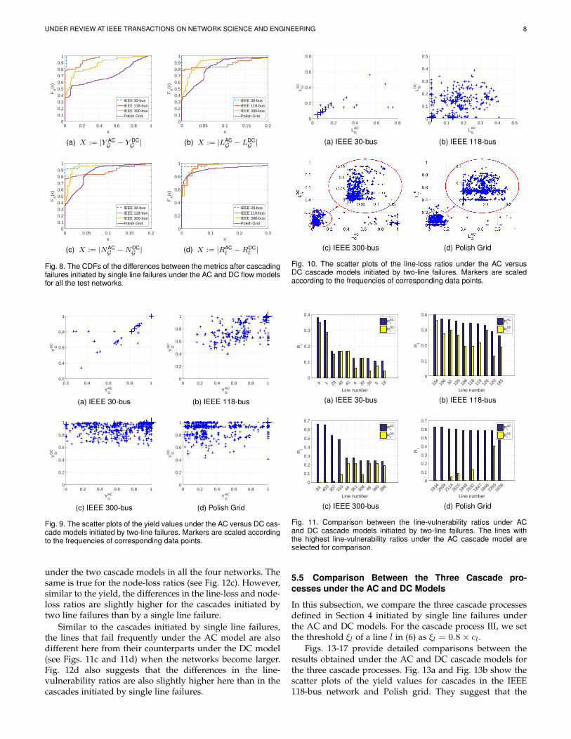
Fig. 9 shows the scatter plot of the yield values underthe AC and DC cascading failures models for the four testnetworks: Yield values obtained by the DC cascade modelare usually higher, specially for large networks. Fig. 12apresents the CDFs of the differences in yield values forall the test networks. Removal of two lines usually putsthe system in a more critical condition with more cascadestages: The magnitudes of the differences in the obtainedyield values are slightly higher for the cascades initiated bytwo line failures than by one line failure.

Fig. 10 and Fig. 12b show the line-loss ratios are still close


0 0.2 0.4 0.6 0.8 1x

0

0.1

0.2

0.3

0.4

0.5

0.6

0.7

0.8

0.9

1F

X(x

)


(a) X := |Y ACG − Y DC

G |

0 0.05 0.1 0.15 0.2x

0

0.1

0.2

0.3

0.4

0.5

0.6

0.7

0.8

0.9

1

FX(x

)


(b) X := |LACG − L

DCG |

0 0.05 0.1 0.15 0.2x

0

0.1

0.2

0.3

0.4

0.5

0.6

0.7

0.8

0.9

1

FX(x

)


(c) X := |NACG −N

DCG |

0 0.1 0.2 0.3x

0

0.2

0.4

0.6

0.8

1F

X(x

)


(d) X := |RACl −R

DCl |

Fig. 8. The CDFs of the differences between the metrics after cascadingfailures initiated by single line failures under the AC and DC flow modelsfor all the test networks.

0.2 0.4 0.6 0.8 1

YGAC

0.2

0.4

0.6

0.8

1

YGD

C

(a) IEEE 30-bus

0 0.2 0.4 0.6 0.8 1

YGAC

0

0.2

0.4

0.6

0.8

1

YGD

C

(b) IEEE 118-bus

0 0.2 0.4 0.6 0.8 1

YGAC

0

0.2

0.4

0.6

0.8

1

YGD

C

(c) IEEE 300-bus

0 0.2 0.4 0.6 0.8 1

YGAC

0

0.2

0.4

0.6

0.8

1

YGD

C

(d) Polish Grid

Fig. 9. The scatter plots of the yield values under the AC versus DC cas-cade models initiated by two-line failures. Markers are scaled accordingto the frequencies of corresponding data points.

under the two cascade models in all the four networks. Thesame is true for the node-loss ratios (see Fig. 12c). However,similar to the yield, the differences in the line-loss and node-loss ratios are slightly higher for the cascades initiated bytwo line failures than by a single line failure.

Similar to the cascades initiated by single line failures,the lines that fail frequently under the AC model are alsodifferent here from their counterparts under the DC model(see Figs. 11c and 11d) when the networks become larger.Fig. 12d also suggests that the differences in the line-vulnerability ratios are also slightly higher here than in thecascades initiated by single line failures.

0 0.2 0.4 0.6 0.8

LGAC

0

0.2

0.4

0.6

0.8

L GDC

(a) IEEE 30-bus

0 0.1 0.2 0.3 0.4 0.5

LGAC

0

0.1

0.2

0.3

0.4

0.5

L GDC

(b) IEEE 118-bus


Fig. 10. The scatter plots of the line-loss ratios under the AC versusDC cascade models initiated by two-line failures. Markers are scaledaccording to the frequencies of corresponding data points.

9 1 28 40 41 4 30 36 5 18

Line number

0

0.1

0.2

0.3

0.4

Rl

RlAC

RlDC

(a) IEEE 30-bus

104

106

30

105

108

116

119

126

120

185

Line number

0

0.1

0.2

0.3

0.4

Rl

RlAC

RlDC

(b) IEEE 118-bus

83

403

307

310

44

361

308

48

360

386

Line number

0

0.1

0.2

0.3

0.4

0.5

0.6

0.7

Rl

RlAC

RlDC

(c) IEEE 300-bus

1934

2608

2114

2620

1848

2592

1847

1846

2293

1656

Line number

0

0.1

0.2

0.3

0.4

0.5

0.6

0.7R

l

RlAC

RlDC

(d) Polish Grid

Fig. 11. Comparison between the line-vulnerability ratios under ACand DC cascade models initiated by two-line failures. The lines withthe highest line-vulnerability ratios under the AC cascade model areselected for comparison.

5.5 Comparison Between the Three Cascade pro-cesses under the AC and DC Models

In this subsection, we compare the three cascade processesdefined in Section 4 initiated by single line failures underthe AC and DC models. For the cascade process III, we setthe threshold ξl of a line l in (6) as ξl = 0.8× cl.

Figs. 13-17 provide detailed comparisons between theresults obtained under the AC and DC cascade models forthe three cascade processes. Fig. 13a and Fig. 13b show thescatter plots of the yield values for cascades in the IEEE118-bus network and Polish grid. They suggest that the


0 0.2 0.4 0.6 0.8 1x

0

0.1

0.2

0.3

0.4

0.5

0.6

0.7

0.8

0.9

1F

X(x

)



G |

0 0.1 0.2 0.3x

0

0.1

0.2

0.3

0.4

0.5

0.6

0.7

0.8

0.9

1

FX(x

)


(b) X := |LACG − L

DCG |

0 0.1 0.2 0.3x

0

0.1

0.2

0.3

0.4

0.5

0.6

0.7

0.8

0.9

1

FX(x

)


(c) X := |NACG −N

DCG |

0 0.1 0.2 0.3 0.4 0.5x

0

0.2

0.4

0.6

0.8

1F

X(x

)


(d) X := |RACl −R

DCl |

Fig. 12. The CDFs of the differences between the metrics after cas-cading failures initiated by two-line failures under the AC and DC flowmodels for all the test networks.

yield values obtained by the cascade process II are generallylower than the other two cascade processes under the ACmodel. Fig. 17a and Fig. 17b, which present the CDFs of thedifferences in yield values under the AC and DC cascademodels for the three cascade processes in the IEEE 118-busnetwork and Polish grid, also show that the differences inthe obtained yield values under the AC and DC models cangrow high for the cascade process II.

Fig. 14a and Fig. 14b show the scatter plots of the line-loss ratios under the AC and DC cascade models for thethree cascade processes in the IEEE 118-bus network andPolish grid. Line-loss ratios obtained by the cascade processII are usually higher, leading to higher differences betweenthe line-loss ratios obtained by the AC and DC flow models.Fig. 17c and Fig. 17d present the CDFs of the differencesin line-loss ratios in the IEEE 118-bus network and Polishgrid. Similar to Fig. 17a and Fig. 17b, the magnitudes of thedifferences in the obtained line-loss ratios under the AC andDC models are highest for the cascade process II.

Fig. 15a and Fig. 15b present the comparison betweenthe highest line-vulnerability ratios under the AC and DCcascade models for the cascade process II in the IEEE 118-bus network and Polish grid. Fig. 16a and Fig. 16b presentthe comparison between the highest line-vulnerability ratiosunder the the AC and DC cascade models for the cascadeprocess III in the IEEE 118-bus network and Polish grid. Thedifference between the individual line-vulnerability ratiosin Fig. 16b is particularly high for the cascade processIII. Fig. 17e and Fig. 17f show that the differences in theline-vulnerability ratios may be quite large for the cascadeprocess III.

Figs. 13-17 suggest that different rules for the supply anddemand balancing and line outages could have differenteffect on the evaluation of the cascades under the ACand DC flow models. In particular, the cascade process IIincreases the differences between the AC and DC models

0 0.1 0.2 0.3 0.4 0.5 0.6 0.7 0.8 0.9 1

YGAC

0

0.1

0.2

0.3

0.4

0.5

0.6

0.7

0.8

0.9

1

YGD

C

Cascade Process ICascade Process IICascade Process III

(a) IEEE 118-bus (b) Polish Grid

Fig. 13. The scatter plots of the yield values under the AC vs DC cascademodels for the three cascade processes initiated by single line failures.Markers are scaled according to the frequencies of corresponding datapoints.

0 0.2 0.4 0.6 0.8

LGAC

0

0.2

0.4

0.6

0.8

L GDC


(a) IEEE 118-bus (b) Polish Grid

Fig. 14. The scatter plots of the line-loss ratios under the AC vs DCcascade models for the three cascade processes initiated by single linefailures. Markers are scaled according to the frequencies of correspond-ing data points.

the most. In this model, by disconnecting many small-sizedgenerators distributed in the network, the demands aresupplied by few large-sized generators during the cascadestages. Consequently, the remaining network suffers fromlow voltage magnitudes and overloaded lines, which canlead to divergence in iterations of AC power flow equations.Moreover, the reactive power flows and voltage magnitudesare not modeled by the DC flow model which can lead tohigher differences between the cascades under AC and DCflow models.

Although the cascade process III does not affect the yieldvalues and line-loss ratios very much, its effect is moresignificant in identifying the most vulnerable set of lines.Due to the probabilistic line tripping model in (6), differentlines may trip at each cascade stage, which can result indetecting different sets of vulnerable lines under AC andDC flow models.

5.6 Main Lessons Learned from the Simulations

In this section, we summarize the results obtained in theprevious subsections. The main lessons learned from theanalysis of the DC cascading failures model compared tothe AC cascading failures model from the simulations are asfollows:

1) When there are no failures and the assumptionsunderlying the DC power flow approximation arevalid, the DC power flow model can approximatethe AC power flow model in the network relativelywell.


104

105

106

30

19

Line number

0

0.1

0.2

Rl

RlAC

RlDC

(a) IEEE 118-bus

1059

2536

2608

643

2592

Line number

0

0.1

0.2

0.3

0.4

0.5

0.6

0.7

Rl

RlAC

RlDC

(b) Polish Grid

Fig. 15. Comparison between the line-vulnerability ratios under the ACand DC cascade models for the cascade process II initiated by singleline failures. The lines with the highest line-vulnerability ratios under theAC cascade model are selected for comparison.

105

106

30

104

108

Line number

0

0.1

0.2

Rl

RlAC

RlDC

(a) IEEE 118-bus

1649

2620

1857

2271

1934

Line number

00.10.20.30.40.50.60.70.80.9

1

Rl

RlAC

RlDC

(b) Polish Grid

Fig. 16. Comparison between the line-vulnerability ratios under the ACand DC cascade models for the cascade process III initiated by singleline failures. The lines with the highest line-vulnerability ratios under theAC cascade model are selected for comparison.

2) The DC power flow model can capture the instanteffects of a single line failure on the flow changes onother lines (i.e., line flow change ratios and line out-age distribution factors) relatively accurately. How-ever, because of their limitations, they fail to captureother dynamics such as node voltage changes andpower loss change ratios.

3) The AC and DC cascade models with the cascadeprocess I provide similar line- and node-loss ratios(i.e., total number of line and node failures) most ofthe time.

4) The AC and DC cascade models with the cascadeprocess I provide similar yield for small networks.However, for large networks (e.g., the Polish grid)the DC cascade model tends to overestimate theyield.

5) The AC and DC cascade models with the cascadeprocess I agree on the most vulnerable lines underthe line-vulnerability ratios in small networks, mostof the time. However, for larger networks (i.e., thePolish grid) they tend to detect different sets of lines.

6) The DC cascade model with the cascade process IIcould underestimate the severity of the cascadecompared to AC model with the same cascadeprocess, as the effects of node voltage changes andreactive power flows are neglected under the DCflow model.

7) The AC and DC cascade models with the cascadeprocess III provide similar yield, line-loss, and vul-nerability ratios for small networks. However, for

0 0.2 0.4 0.6 0.8 1x

0.2

0.3

0.4

0.5

0.6

0.7

0.8

0.9

1

FX(x

)


IEEE 118-bus


G |

0 0.2 0.4 0.6 0.8 1x

0

0.1

0.2

0.3

0.4

0.5

0.6

0.7

0.8

0.9

1

FX(x

)


Polish Grid

(b) X := |Y ACG − Y DC

G |

0 0.2 0.4 0.6 0.8 1x

0.2

0.3

0.4

0.5

0.6

0.7

0.8

0.9

1

FX(x

)


IEEE 118-bus

(c) X := |LACG − L

DCG |

0 0.2 0.4 0.6 0.8 1x

0

0.1

0.2

0.3

0.4

0.5

0.6

0.7

0.8

0.9

1

FX(x

)


Polish Grid

(d) X := |LACG − L

DCG |

0 0.05 0.1 0.15 0.2x

0.2

0.4

0.6

0.8

1

FX(x

)


IEEE 118-bus

(e) X := |RACl −R

DCl |

0 0.2 0.4 0.6 0.8 1x

0

0.2

0.4

0.6

0.8

1

FX(x

)


Polish Grid

(f) X := |RACl −R

DCl |

Fig. 17. The CDFs of the differences between the metrics after cascadesunder the AC and DC models for the three cascade processes initiatedby single line failures in IEEE 118-bus network and Polish grid.

larger networks (e.g., the Polish grid) they result indifferent sets of most vulnerable lines.

Overall, the obtained results suggest that due to the volt-age constraints, the divergence problems, and the reactivepower flows, the cascades under the AC flow models aremore significant compared to the ones under the DC flowmodel. Hence, the DC model may underestimate the sever-ity of the cascade, especially for larger networks.

6 CONCLUSION

In this paper, we thoroughly compared the AC and DCpower flow models in describing the state of the grid whenthere are no failures as well as in predicting the effectof single line failures and the evolution of cascades. Wenumerically compared the AC and DC power flow modelsand demonstrate that when there are no failures, the DCpower flow model provides relatively accurate approxima-tion of the AC power flow model. Moreover, we providedan upperbound on the difference between the active powerflow on a line under the AC and DC flow models.

Upon failures, numerical results for the single line failureanalysis show that the DC power flow model provides asimilar flow redistribution after single line failures as theAC flow model. On the other hand, the cascading failures


simulation demonstrates that even slight errors in individ-ual line flows can turn out to be important at cascade stages,and the metrics that capture the operational and topologicalaspects of the cascade can differ significantly under the twomodels. These results suggest that special care should betaken when drawing conclusions based on the DC cascademodel in power grids. Overall, the DC cascade model canprovide an overly optimistic estimation compared to the ACcascade model.

ACKNOWLEDGEMENT

This work was supported in part by Alliander N.V., DARPARADICS under contract #FA-8750-16-C-0054, funding fromthe U.S. DOE OE as part of the DOE Grid ModernizationInitiative, and DTRA grant HDTRA1-13-1-0021. The workof G.Z. was also supported in part by the Blavatnik ICRC.

REFERENCES

[1] J. J. Grainger and W. D. Stevenson, Power system analysis.McGraw-Hill, 1994.

[2] R. Baldick, B. Chowdhury, I. Dobson, Z. Dong, B. Gou,D. Hawkins, H. Huang, M. Joung, D. Kirschen, F. Li et al., “Initialreview of methods for cascading failure analysis in electric powertransmission systems IEEE PES CAMS task force on understand-ing, prediction, mitigation and restoration of cascading failures,”in Proc. IEEE PES-GM’08, July 2008.

[3] Entsoe, “Report on blackout in Turkey on 31st March 2015,” Tech.Rep., 2015. [Online]. Available: http:/www.entsoe.eu/

[4] A. Bakshi, A. Velayutham, S. Srivastava, K. Agrawal, R. Nayak,S. Soonee, and B. Singh, “Report of the enquiry committee on griddisturbance in Northern Region on 30th july 2012 and in Northern,Eastern & North-Eastern Region on 31st July 2012,” New Delhi,India, 2012.

[5] “Final report on the august 14th blackout in the united statesand canada: Causes and recommendations,” U.S.- Canada PowerSystem Outage Task Force, Tech. Rep., April 2004.

[6] F. Alvarado and S. Oren, “Transmission system operation andinterconnection,” National transmission grid study–Issue papers, pp.A1–A35, 2002.

[7] D. Bienstock, Electrical Transmission System Cascades and Vulnerabil-ity: An Operations Research Viewpoint. SIAM, 2016, vol. 22.

[8] P. Crucitti, V. Latora, and M. Marchiori, “A topological analysis ofthe italian electric power grid,” Physica A: Statistical Mechanics andits Applications, vol. 338, no. 1, pp. 92–97, 2004.

[9] Y. Koc, T. Verma, N. A. Araujo, and M. Warnier, “Matcasc: A toolto analyse cascading line outages in power grids,” in Proc. IEEEIWIES’13, 2013.

[10] S. Soltan, D. Mazauric, and G. Zussman, “Analysis of failures inpower grids,” to appear in IEEE Trans. Control Netw. Syst. (availableon IEEE Xplore Digital Library), 2017.

[11] K. Purchala, L. Meeus, D. Van Dommelen, and R. Belmans, “Use-fulness of DC power flow for active power flow analysis,” in IEEEPES-GM’05, June 2005.

[12] D. Van Hertem, J. Verboomen, K. Purchala, R. Belmans, andW. Kling, “Usefulness of dc power flow for active power flowanalysis with flow controlling devices,” in Proc. IET ACDC’06,2006, pp. 58–62.

[13] I. Dobson, Encyclopedia of Systems and Control, ser. Cascadingnetwork failure in power grid blackouts. Springer, 2015.

[14] P. Hines, K. Balasubramaniam, and E. C. Sanchez, “Cascadingfailures in power grids,” IEEE Potentials, vol. 28, no. 5, pp. 24–30,2009.

[15] P. D. Hines and P. Rezaei, “Cascading failures in power systems,”Smart Grid Handbook, 2016.

[16] S. V. Buldyrev, R. Parshani, G. Paul, H. E. Stanley, and S. Havlin,“Catastrophic cascade of failures in interdependent networks,”Nature, vol. 464, no. 7291, pp. 1025–1028, 2010.

[17] H. Xiao and E. M. Yeh, “Cascading link failure in the power grid:A percolation-based analysis,” in Proc. IEEE Int. Work. on SmartGrid Commun., June 2011.

[18] D. P. Chassin and C. Posse, “Evaluating North American electricgrid reliability using the Barabasi–Albert network model,” PhysicaA, vol. 355, no. 2-4, pp. 667 – 677, 2005.

[19] B. A. Carreras, V. E. Lynch, I. Dobson, and D. E. Newman, “Criticalpoints and transitions in an electric power transmission model forcascading failure blackouts,” Chaos, vol. 12, no. 4, pp. 985–994,2002.

[20] B. A. Carreras, V. E. Lynch, I. Dobson, and D. E. Newman,“Complex dynamics of blackouts in power transmission systems,”Chaos, vol. 14, no. 3, pp. 643–652, 2004.

[21] M. Anghel, K. A. Werley, and A. E. Motter, “Stochastic model forpower grid dynamics,” in Proc. HICSS’07, Jan. 2007.

[22] Y. Koc, M. Warnier, P. Van Mieghem, R. E. Kooij, and F. M. Brazier,“The impact of the topology on cascading failures in a power gridmodel,” Physica A: Statistical Mechanics and its Applications, vol.402, pp. 169–179, 2014.

[23] A. Asztalos, S. Sreenivasan, B. K. Szymanski, and G. Korniss,“Cascading failures in spatially-embedded random networks,”PloS one, vol. 9, no. 1, p. e84563, 2014.

[24] J. Chen, J. S. Thorp, and I. Dobson, “Cascading dynamics andmitigation assessment in power system disturbances via a hiddenfailure model,” Int. J. Elec. Power and Ener. Sys., vol. 27, no. 4, pp.318 – 326, 2005.

[25] A. Moussawi, N. Derzsy, X. Lin, B. K. Szymanski, and G. Ko-rniss, “Limits of predictability of cascading overload failuresin spatially-embedded networks with distributed flows,” arXivpreprint arXiv:1706.04579, 2017.

[26] A. Bernstein, D. Bienstock, D. Hay, M. Uzunoglu, and G. Zussman,“Power grid vulnerability to geographically correlated failures -analysis and control implications,” in Proc. IEEE INFOCOM’14,Apr. 2014.

[27] D. Bienstock, “Optimal control of cascading power grid failures,”Proc. IEEE CDC-ECC, Dec. 2011.

[28] R. Pfitzner, K. Turitsyn, and M. Chertkov, “Controlled trippingof overheated lines mitigates power outages,” ArXiv preprint, no.1104.4558, Oct. 2011.

[29] P. D. Hines, I. Dobson, E. Cotilla-Sanchez, and M. Eppstein, “”dualgraph” and ”random chemistry” methods for cascading failureanalysis,” in Proc. IEEE HICSS’13, 2013.

[30] D. P. Nedic, I. Dobson, D. S. Kirschen, B. A. Carreras, and V. E.Lynch, “Criticality in a cascading failure blackout model,” Int. J.Elec. Power, vol. 28, no. 9, pp. 627–633, 2006.

[31] M. Papic, K. Bell, Y. Chen, I. Dobson, L. Fonte, E. Haq, P. Hines,D. Kirschen, X. Luo, S. Miller et al., “Survey of tools for riskassessment of cascading outages,” in IEEE PES-GM’11, 2011.

[32] R. D. Zimmerman, C. E. Murillo-Sanchez, and R. J. Thomas,“Matpower: Steady-state operations, planning, and analysis toolsfor power systems research and education,” IEEE Trans. PowerSyst., vol. 26, no. 1, pp. 12–19, 2011.

[33] R. Kaye and F. Wu, “Analysis of linearized decoupled power flowapproximations for steady-state security assessment,” IEEE Trans.Circuits and Sys., vol. 31, no. 7, pp. 623–636, 1984.

[34] T. J. Overbye, X. Cheng, and Y. Sun, “A comparison of the ACand DC power flow models for LMP calculations,” in Proc. IEEEHICSS’04, 2004.

[35] P. Yan and A. Sekar, “Study of linear models in steady state loadflow analysis of power systems,” in IEEE PES-WM’02, Jan. 2002.

[36] B. Stott, J. Jardim, and O. Alsac, “DC power flow revisited,” IEEETrans. Power Syst., vol. 24, no. 3, pp. 1290–1300, 2009.

[37] S. Deckmann, A. Pizzolante, A. Monticelli, B. Stott, and O. Alsac,“Numerical testing of power system load flow equivalents,” IEEETrans. Power App. and Sys., no. 6, pp. 2292–2300, 1980.

[38] “Power systems test case archive,” available at:http://www.ee.washington.edu/research/pstca/.

[39] J. D. Glover, M. S. Sarma, and T. Overbye, Power System Analysis& Design, SI Version. Cengage Learning, 2012.

[40] H. Cetinay, F. A. Kuipers, and P. Van Mieghem, “A topologicalinvestigation of power flow,” to appear in IEEE Systems Journal,2017.

[41] A. J. Wood and B. F. Wollenberg, Power generation, operation, andcontrol, 3rd ed. John Wiley & Sons, 2012.

[42] N. Biggs, Algebraic graph theory. Cambridge university press, 1993.


Hale Cetinay is pursuing her Ph.D. sinceSeptember 2014 at Delft University of Technol-ogy, The Netherlands. She obtained her M.Sc.degree (May, 2014) in Electrical and Electron-ics Engineering at Middle East Technical Uni-versity, Turkey, where she also received herB.Sc. degree (June, 2011). Her main researchinterests include network science, electrical net-works, and smart grids.

Saleh Soltan is a Ph.D. candidate in the de-partment of Electrical Engineering at ColumbiaUniversity. He received B.S. degrees in Electri-cal Engineering and Mathematics (double ma-jor) from Sharif University of Technology, Iran in2011 and the M.S. degree in Electrical Engineer-ing from Columbia University in 2012. He is theGold Medalist of the 23rd National MathematicsOlympiad in Iran in 2005 and the recipient ofColumbia University Electrical Engineering Arm-strong Memorial Award in 2012.

Fernando A. Kuipers is an associate professorworking on Internet Science at Delft Universityof Technology (TU Delft). In 2004, he obtainedhis Ph.D. degree cum laude; the highest possibledistinction at TU Delft. His research focus is onnetwork optimization, network resilience, Qualityof Service, and Quality of Experience and ad-dresses problems in software-defined network-ing, optical networking, content distribution, andcyber-physical systems/infrastructures. His workon these subjects include distinguished papers

at IEEE INFOCOM 2003, Chinacom 2006, IFIP Networking 2008, IEEEFMN 2008, IEEE ISM 2008, ITC 2009, IEEE JISIC 2014, and NetGames2015. Fernando Kuipers is senior member of the IEEE, was a visit-ing scholar at Technion - Israel Institute of Technology (in 2009) andColumbia University in the City of New York (in 2016), and is boardmember of the IEEE Benelux chapter on communications and vehiculartechnology and of the Royal Netherlands Society of Engineers (KIVI),section Telecommunication.

Gil Zussman received the Ph.D. degree in elec-trical engineering from the Technion in 2004 andwas a postdoctoral associate at MIT in 2004-2007. He is currently an Associate Professorof Electrical Engineering at Columbia University.He is a co-recipient of 7 paper awards includingthe ACM SIGMETRICS06 Best Paper Award,the 2011 IEEE Communications Society Awardfor Advances in Communication, and the ACMCoNEXT’16 Best Paper Award. He received theFulbright Fellowship, the DTRA Young Investi-

gator Award, and the NSF CAREER Award, and was a member of ateam that won first place in the 2009 Vodafone Foundation WirelessInnovation Project competition.

Piet Van Mieghem received the Masters(magna cum laude, 1987) and PhD (summa cumlaude, 1991) degrees in electrical engineeringfrom the K.U. Leuven, Leuven, Belgium. He isa Professor at the Delft University of Technologyand Chairman of the section Network Architec-tures and Services (NAS) since 1998. His mainresearch interests lie in modeling and analysisof complex networks and in new Internet-likearchitectures and algorithms for future communi-cations networks. Before joining Delft, he worked

at the Interuniversity Micro Electronic Center (IMEC) from 1987 to1991. During 1993-1998, he was a member of the Alcatel CorporateResearch Center in Antwerp, Belgium. He was a visiting scientist at MIT(1992-1993), a visiting professor at UCLA (2005), a visiting professorat Cornell University (2009), and at Stanford University (2015). He isthe author of four books: Performance Analysis of CommunicationsNetworks and Systems (Cambridge Univ. Press, 2006), Data Com-munications Networking (Techne, 2011), Graph Spectra for ComplexNetworks (Cambridge Univ. Press, 2011), and Performance Analysis ofComplex Networks and Systems (Cambridge Univ. Press, 2014).


APPENDIXTHE DC POWER FLOWS ACCURACY

As mentioned in Section 3.2, the DC power flow modelprovides a good approximation of the AC power flow modelunder three conditions. Here, we provide analytical insightson the accuracy of the DC power flow model.

In the following lemma, we provide an upper bound onthe difference between the AC active power flows P (AC)

ij andthe DC active power flows P (DC)

ij under those conditions.Lemma 1. Assume the three conditions for validity of the DC

power flow as a linear approximation for the AC powerflow hold within following bounds:

1) |θi − θj | ≤ εθ,∀{i, j} ∈ L,2) |gij/bij | ≤ εg,∀{i, j} ∈ L,3) ||Vi| − 1| ≤ εv,∀i ∈ N ,

for εθ, εv, εg < 1. Then, for any 1 ≤ i, j ≤ n:

|P (AC)ij − P (DC)

ij | ≤ ε‖B‖1 + ‖P− P‖1, (9)

in which ε := 2εg + 4εvεg + 2ε2vεg + 2εvεθ + ε2vεθ + ε3θ and‖B‖1 :=

∑ni=1

∑nj=1 |bij |.

Proof: Using the definition of the apparent powerSik = P (AC)

ik + iQ(AC)ik in (1), we have:

P (AC)ij = <

{Vi((Vi − Vj)(gij + ibij)

)∗}= <

{(|Vi|2 − |Vi||Vj |ei(θi−θj))(gij − ibij)

}= |Vi|2gij − |Vi||Vj |gij cos(θi − θj)− |Vi||Vj |bij sin(θi − θj).

Define θi − θj := αij and |Vi| := 1 + βi. Then:

||Vi|2gij | = |gij + (2βi + β2i )gij |

≤ |bij |(εg + 2εvεg + ε2vεg).

Moreover, using | cos(x)| ≤ 1:

||Vi||Vj |gij cos(αij)| ≤ |gij + (βi + βj + βiβj)gij |≤ |bij |(εg + 2εvεg + ε2vεg).

Using sin(x) = x + F (x), for F (x) := −x3/6 + O(x5), wealso have:

− |Vi||Vj |bij sin(θi − θj) =

= −bij(θi − θj)− bij

((βi + βj + βiβj)(θi − θj)+F ((θi − θj)3)|Vi||Vj |

),

in which:

| − bij((βi + βj + βiβj)(θi − θj)+F ((θi − θj)3)|Vi||Vj |

)| ≤

≤ |bij |(2εvεθ + ε2vεθ + ε3θ/6 + ε3θεv/3 + ε3θε

2v/6)

≤ |bij |(2εvεθ + ε2vεθ + ε3θ).

Hence,

P (AC)ij = −bij(θi − θj) + eij , (10)

in which:

|eij | ≤ |bij |(2εg + 4εvεg + 2ε2vεg + 2εvεθ + ε2vεθ + ε3θ

).

Notice that −bij(θi − θj) is not necessarily equal to P (DC)ij =

−bij(θi−θj) since θi and θj are obtained from the AC power

flow model, which are different from the phase anglesobtained by the DC power flow model. However, we cancompute the difference between these two values by writingthe power flow equations using (10) as follows:

AC:−BΘ + E = P

−BΘ = P−E + (P− P)

DC:−BΘ = P

in which E is an n × 1 vector with the ith entry equalto ei such that |ei| ≤

∑j∈N(i) |eij |. Recall that vectors P

and P are equal except (depending on the lossless assump-tion) in the slack bus (first entry). From the flow equationsand the superpositions principle, the difference between−bij(θi − θj) and −bij(θi − θj) cannot be greater than themaximum flow that vector E− (P− P) can produce whichis at most ‖P− P‖1 + (

∑ni=1

∑j∈N(i) |bij |)(2εg + 4εvεg +

2ε2vεg + 2εvεθ + ε2vεθ + ε3θ). Hence, a conservative bound forthe difference between the AC and DC active power flowsis:


ij | ≤ ε‖B‖1 + ‖P− P‖1.

The following corollaries, which immediately followfrom Lemma 1, demonstrate the bounds for the differencebetween the AC and DC active power flows for the specialcases of a lossless network (i.e., εg = 0).Corollary 1. If the lines are lossless (εg = 0), then for any

1 ≤ i, j ≤ n:


ij | ≤ (2εvεθ + ε2vεθ + ε3θ)‖B‖1.

Corollary 2. If the lines are lossless (εg = 0), and for all thelines bij = −1, then for any 1 ≤ i, j ≤ n:


ij | ≤ 4(2εvεθ + ε2vεθ + ε3θ)|L|.

In the following proposition, we demonstrate that if thepower network topology is a tree, we can improve thebound in Corollary 1 and prove that the DC power flowsare equal to the AC active power flows.Proposition 1. If G is a tree and εg = 0, then ∀1 ≤ i, j ≤ n :

P (AC)ij = P (DC)

ij .

Proof: We want to show that P (DC)ij = P (AC)

ij ,∀{i, j} ∈L is a DC power flow solution for this instance. As allthe lines are purely reactive, the network is lossless andin the AC power flows |P (AC)

ij | = |P (AC)ji |,∀{i, j} ∈ L.

From Kirchhoff’s laws, we also have∑j∈N(i) P

(AC)ij = Pi.

Hence, setting P (DC)ij = P (AC)

ij completely satisfies the activepower flow conservation in equation (4). It remains to provethat there are phase angles satisfying equation (4) withP (DC)ij = P (AC)

ij . Since G is a tree, m = n − 1. Hence,P (DC)ij = −bij(θi− θj) for all {i, j} ∈ L consists of n−1 inde-

pendent linear equations for n variables θ1, θ2, . . . , θn (It isknown that for a connected graph G, rank(B) = n− 1 [42]).As a result, by choosing θ1 = 0, all other phase angles canbe found uniquely. Hence, P (DC)

ij = P (AC)ij is the DC power

flow solution for this instance as well.

UNDER REVIEW AT IEEE TRANSACTIONS ON NETWORK...

Documents

Transcript of UNDER REVIEW AT IEEE TRANSACTIONS ON NETWORK...