
UNCLASSIFIED AD 406 608 - DTIC
167
UNCLASSIFIED AD 406 608 DEFENSE DOCUMENTATION CENTER FOR SCIENTIFIC AND TECHNICAL INFORMATION CAMERON STATION. ALEXANDRIA. VIRGINIA w UNCLASSIFIED
Transcript of UNCLASSIFIED AD 406 608 - DTIC

UNCLASSIFIED
AD 406 608
DEFENSE DOCUMENTATION CENTERFOR
SCIENTIFIC AND TECHNICAL INFORMATION
CAMERON STATION. ALEXANDRIA. VIRGINIA
wUNCLASSIFIED
NOTICE: When government or other drawings, speci-fications or other data are used for any purposeother than in connection with a definitely relatedgovernment procurement operation, the U. S.Government thereby incurs no responsibility, nor anyobligation whatsoever; and the fact that the Govern-ment may have formulated, furnished, or in any waysupplied the said dravings, specifications, or otherdata is not to be regarded by implication or other-wise as in any manner licensing the holder or anyother person or corporation, or conveying any rightsor permission to manufacture, use or sell anypatented invention that may in any way be relatedthereto.
A Digital-CmueLUL
InvestIigaiol n C !n "i 'Ilia omputer -AiPde d en s ign+° P... .. •roject++ Sta
the Cdneiro Constant-Pu r mllter•+• + ++Electric Network
Computer-Aided Design: A Statement Ross. D. Ta of Objectives
Computr-Aideod Dsin elated to the Coons. . .•j ZEngineering
Design Process Mmann Rt. S.
Investigotions in Computer-Aided Design Project Stan
Autormatic Feodrnte Sottin o in NumericCloyns S. A.++++• iCotktrolled Contour Mili~ng
W ,I Investigations in Computor-Aided Design Coonss, . A.+ f+'+ ;", Roon". G. A
• + +', . (• ~Design of a Remote Display COMlO"eKnl .C
invltla~~n i Cop~o-Aided Design R~oss. D. T_
for Numerica~lly controlled Production Coe .A
An Algorithmic Theory of Langusge Ross. D. T.
DdwfMW f flm*
CDDec 1
oriW m -v ...... :++
Dep.v : EeLa 3ie+s

REPORTS PUBLISHED ON CONTRACT AF-33(600)-42859
REPORT ANDTECHNICAL MEMONUMBERS ASTIA NO. TITLE AUTHOR(S) DATE
8436-TM-1 AD 243 156 Papers on the APT Language Ross, D. T. b/60PB 155 406 Feldmann. C. G.
8436-TM-2 AD 248 436 Method for Computer Visulaisation Smith. A. F. 9/60PB 155 407
8436-TM-3 AD 248 437 A Digital Computer Representation of Meyer. C. S. 8/60PB 155 408 the Linear, Constant-Parameter
Electric Network
8436-TM-4 AD 252 060 Computer-Aided Design: A Statement Rome. D. T 9/60PB 155 409 of Objectives
8436-TM-5 AD 252 061 Computer-Aided Design Related to the Coons, S. A. 10/60PB 155 410 Engineering Design Process Manu, R. S.
8436-'R-1 AD Z52 062 Investigations in Computer-Aided Design Project Staff 1/61PB I55 405
8436-R-1 AD 253 676 Automatic Feedrate Setting in Numerically Welch, J. D. 12/60PB 155 553 Controlled Contour Milling •
8436-IR-2 AD 269 573 Investigations in Computer-Aided Design Rose. D. T. 11/61Coons, S. A.
ESL-R-132 AD 274 985 Design of a Remote Display Console Rand, G. C. 2/62
ESL-IR-138 AD 282 679 Investigatibons in Computer-Aided Design Ross, D. T. 5/62for Numerically Controlled Production Coons, S. A.
ESL-TM-156 AD 296 998 An Algorithmic Theory of Language Ross, D. T. 11/62
ESL-TM-164 Investigations in Computer-Aided Design Rose, D. T. 2/63for Numerically Controlled Production-- Coons, S. A.Interim Technical Progress Report No. 5
ESL-TM-167 Specialized Computer Equipment for Stoth, R. H. 3/63Generation and Display of ThreeDimensional Curvilinear Figures
ESL-TM-169 An Outline of the Requirements for a Coons, S. A. 3/63Computer-Aided Design System
ESLL-TM-170 Theoretical Foundations for the Computer- Rose, D. T. 3/63Aided Design System Rodrigues, J. E.

TECHNICAL MEMORANDUM Copy No._a1
ESL- TM- 167
SPECIALIZED COMPUTER EQUIPMENT FORGENERATION AND DISPLAY OF THREEDIMENSIONAL CURVILINEAR FIGURES
byRobert H. Stots
March, 1963
Contract No. AF-33(600)-42859
The work reported in this document has been made possible through thesupport and sponsorship extended to the Massachusetts Institute ofTechnology, Electronic Systems Laboratory by the ManufacturingTechnology Laboratory, ASD, Wright-Patterson Air Force Base underContract No. AF-33(600)-42859, M.I.T. Project No. DSR 8753. It ispublished for technical information only and does not necessarily re-present recommendations or conclusions of the sponsoring agency.
Approved by:DouglafTT. Ross, Project EngineerHead, Computer Applications Group
Electronic Systems LaboratoryDepartment of Electrical EngineeringMassachusetts Institute of Technology
Cambridge 39, Massachusetts
NOTICES
When Government drawings, specifications, or other data are usedfor any purpose other than in connection with a definitely relatedGovernment procurement operation, the United States Governmenttherebykicures no responsibility nor any obligation whatsoever; andthe fact that the Government may have formulated, furnished, or inany way supplied the said drawings, specifications, or other data,is not to be regarded by implication or otherwise as in any mannerlicensing the holder or any other person or corporation, or conveyingany rights or permission to manufacture, use, or sell any patentedinvention that* may in any way be related thereto.
This document may not be reproduced in any form in whole or in partwithout prior approval of the Aeronautical Systems Division, ASRCTF.
Requests for additional copies by Agencies of the Department of Defense,their contractors, and other Government Agencies should be directed to:
ARMED SERVICES TECHNICAL INFORMATION AGENCYARLINGTON HALL STATIONARLINGTON 12, VIRGINA
Department of Defense contractors must be established for ASTIA ser-vices or have their "need-to-know" certified by the cognizant militaryagency of their project or contract.
Copies of ASD Technical Reports should not be returned to the Aero-nautical Systems Division unless return is required by security con-siderations, contractual obligations, or notice on a specific document.

ABSTRACT
Studies being conducted of Computer-Aided Design of three-dimensionalshaped objects have shown the need for improved graphical man-computercommunications, particularly faster displays. A straight-line -and-curve -
drawing display system is proposed which is capable of drawing two-dimensional, axonometric projections of curvi-linear three-dimensionalfigures at up to 100 times the speed of present point-plotting display scopes.The system, based on digital incremental computing techniques, consistsof a Line Generator to produce time varying x, y, and z pulse-train sig-nals proportional to the numerical input information; a Rotation Matrixto transform these signals into ones in the h and v coordinate axes of thescope; and Accumulating Registers (bi-directional counters) to hold theresultant data for the scope deflection amplifiers. The Line Generatoris capable of producing straight lines and second-order curves of variablelength.
Two basic elements are compared as building blocks for the Line Generatorand Rotation Matrix: the Binary Rate Multiplier (BRM) and the DigitalDifferential Analyzer (DDA). The operating principals of these units aredescribed and their differences as computing elements for this systemare analyzed. The entire system was simulated on a PDP-I computerwhich has a standard display scope and the results of comparative testsbetween DDA- and BRM-drawn figures are shown. Although the BRM haslarger errors than the DDA for equivalent register lengths, its simplicitymakes it attractive. BRM errors are studied in detail, and theoretical andsimulation results for improved BRM's are given.
Additions to the display system permitting generation of stereoscopic andperspective projections are also described, and figures resulting fromsimulations of these systems are shown. It is concluded that a displaysystem with an incremental computing capability will provide a soundbasis for future work in Computer-Aided Design.
iii
ACKNOWLEDGEMENTS
The author would like to thank the members of the Electronic SystemsLaboratory for their assistance and moral support in the work leading to thisthesis. He is indebted to the Messrs. John E. Ward, Frank B. Hills, andDrs. Donald R. Haring and Ivan E. Sutherland for their support and manysuggestions; to Arthur Giordani for his artistic talents and his conscientious-ness; and to the girls who did the typing, Ionia Lewis, Laurel Retajc.yk andMary Berry. In particular the author would like to thank Mr. Douglas T. Rossfor his ideas and encouragement from the start and for his help in the lastcrucial days of writing this manuscript.
iv
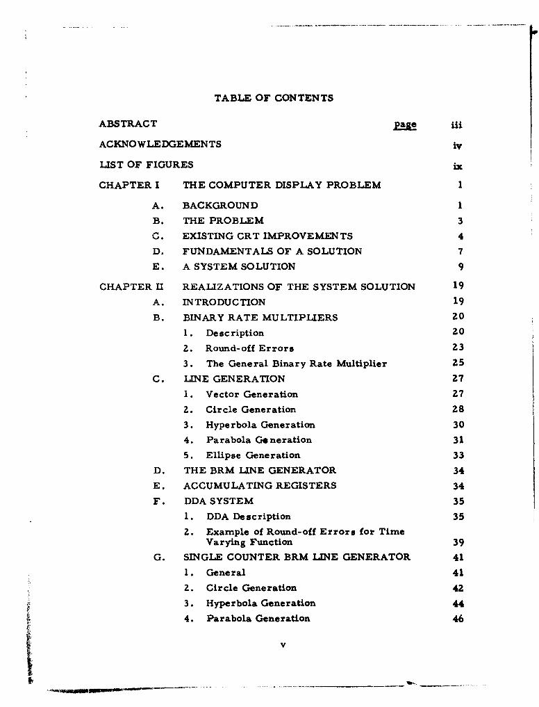
TABLE OF CONTENTS
ABSTRACT page iii
ACKNOWLEDGEMENTS iv
LIST OF FIGURES ix
CHAPTER I THE COMPUTER DISPLAY PROBLEM 1
A. BACKGROUND 1
B. THE PROBLEM 3
C. EXISTING CRT IMPROVEMENTS 4
D. FUNDAMENTALS OF A SOLUTION 7
E. A SYSTEM SOLUTION 9
CHAPTER fl REALIZATIONS OF THE SYSTEM SOLUTION 19
A. INTRODUCTION 19
B. BINARY RATE MULTIPLIERS 20
1. Description 20
2. Round-off Errors Z3
3. The General Binary Rate Multiplier 25
C. LINE GENERATION 27
1. Vector Generation 27
2. Circle Generation 28
3. Hyperbola Generation 30
4. Parabola Go neration 31
5. Ellipse Generation 33
D. THE BRM LINE GENERATOR 34
E. ACCUMULATING REGISTERS 34
F. DDA SYSTEM 35
1. DDA Description 35
2. Example of Round-off Errors for TimeVarying Function 39
G. SINGLE COUNTER BRM LINE GENERATOR 41
1. General 41
2. Circle Generation 42
3. Hyperbola Generation 44
4. Parabola Generation 46
V
L'
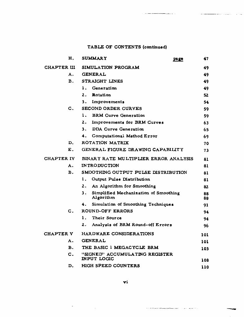
TABLE OF CONTENTS (continued)
H. SUMMARY 47
CHAPTER III SIMULATION PROGRAM 49
A. GENERAL 49B. STRAIGHT LINES 49
1. Generation 49
2. Rotation 52
3. Improvements 54
C. SECOND ORDER CURVES 59
1. BRM Curve Generation 59
2. Improvements for BRM Curves 633. DDA Curve Generation 65
4. Computational Method Error 69
D. ROTATION MATRIX 70
E. GENERAL FIGURE DRAWING CAPABILITY 73
CHAPTER IV BINARY RATE MULTIPLIER ERROR ANALYSIS 81
A. INTRODUCTION 81B. SMOOTHING OUTPUT PULSE DISTRIBUTION 81
1. Output Pulse Distribution 81
2. An Algorithm for Smoothing 82
3. Simplified Mechanization of Smoothing 88Algorithm 88
4. Simulation of Smoothing Techniques 91
C. ROUND-OFF ERRORS 941. Their Source 94
2. Analysis of BRM Round-off Errors 96
CHAPTER V HARDWARE CONSIDERATIONS 101
A. GENERAL 101
B. THE BASIC 1 MEGACYCLE BRM 103
C. "SIGNED" ACCUMULATING REGISTERINPUT LOGIC 108
D. HIGH SPEED COUNTERS 110
vi

TABLE OF CONTENTS (continued)
CHAPTER VI OTHER STUDIES page 117
A. GENERAL 117
B. STEREO PROGRAM 117
C. PERSPECTIVE PROJECTION 124
D. CONCLUSIONS 128
CHAPTER VII CONCLUSIONS AND RECOMMENDATIONS 129
A. THE PROBLEM AND THE SYSTEM SOLUTION 129
B. THE BASIC ELEMENT FOR THE LINEGENERATOR 131
C. MORE SOPHISTICATED PROJECTED DISPLAYS 131
D. OTHER POTENTIALS OF THE SYSTEM 132
E. CRITICISM OF THE SYSTEM 134
APPENDIX A PROGRAM DESCRIPTION 137
APPENDIX B ANALOG SYSTEM 145
BIBLIOGRAPHY 153
vii
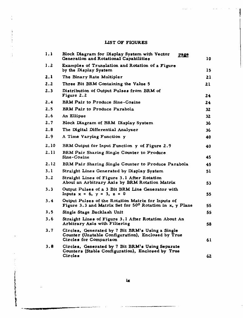
LIST OF FIGURES
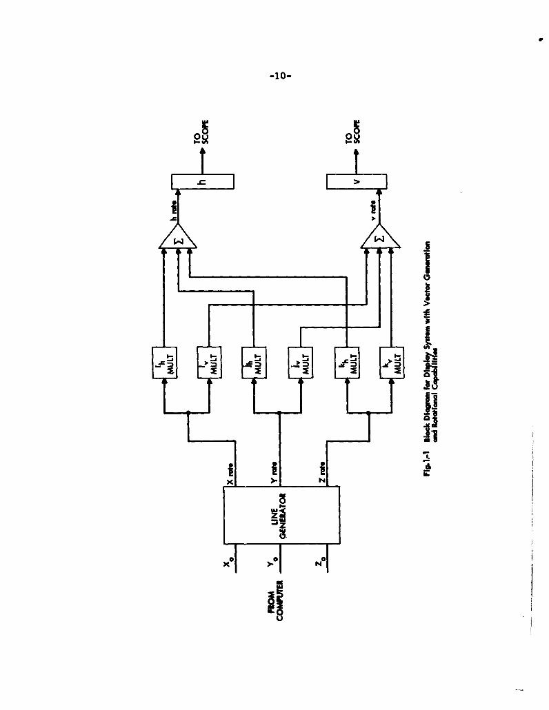
1.1 Block Diagram for Display System with Vector pageGeneration and Rotational Capabilities 10
1.2 Examples of Translation and Rotation of a Figureby the Display System 15
2.1 The Binary Rate Multipler 21
2.2 Three Bit BRM Containing the Value 5 21
2.3 Distribution of Output Pulses from BRM ofFigure 2.2 24
2.4 BRM Pair to Produce Sine-Cosine 24
2.5 BRM Pair to Produce Parabola 32
2.6 An Ellipse 32
2.7 Block Diagram of BRM Display System 36
2.8 The Digital Differential Analyzer 36
2.9 A Time Varying Function y 40
2.10 BRM Output for Input Function y of Figure 2.9 40
2.11 BRM Pair Sharing Single Counter to ProduceSine-Cosine 45
2.12 BRM Pair Sharing Single Counter to Produce Parabola 45
3.1 Straight Lines Generated by Display System 51
3.2 Straight Lines of Figure 3.1 After RotationAbout an Arbitrary Axis by BRM Rotation Matrix 53
3.3 Output Pulses of a 3 Bit BRM Line Generator withInputs x = 6, y = 3, z = 0 55
3.4 Output Pulses of the Rotation Matrix for Inputs ofFigure 3.3 and Matrix Set for 500 Rotation in x, y Plane 55
3.5 Single Stage Backlash Unit 55
3.6 Straight Lines of Figure 3.1 After Rotation About AnArbitrary Axis with Filtering 58
3.7 Circles, Generated by 7 Bit BRM's Using a SingleCounter (Unstable Configuration), Enclosed by TrueCircles for Comparison 61
3.8 Circles, Generated by 7 Bit BRM's Using SeparateCounters (Stable Configuration), Enclosed by TrueCircles 62
ix
LIST OF FIGURES (continued)
3.9 Multiple Circles Generated by BRM's Using VaryingInitial Conditions on Their Single Counter (UnstableConfiguration) 64
3.10 Multiple Circles Generated by BRM's Using VaryingInitial Conditions on Their Single Counter (UnstableConfiguration) 66
3.11 Circles, Generated by BRM's and DDA's (StableConfiguration) Enclosed by True Circles 67
3.12 Expanded View of Arcs of Circles Generated by BRM'sand DDA's (Stable Configuration) 68
3.13 Tetrahedron, Generated by BRM's, After Rotation AboutAn Arbitrary Axis by Rotation Matrix Consisting of BRM'sof Various Lengths 71
3.14 Figures Generated by Display System 74
3.15 Breakdown of Lines Used to Produce Figure 3.14 (c) 75
3.16 Breakdown of Lines Used to Produce Figure 3.14 (b) 75
3.17 Figures, Generated by Display System Using a BRMLine Generator, Shown to the Scale of the Display Scope 78
4.1 Distribution of Output Pulses for 4 Bit BRM Containingthe Value 5 83
4.2 A Smoothed Distribution of Output Pulses for Figure 4.1 83
4.3 K Bit BRM Containing Some Arbitrary Value 85
4.4 Distribution of Sampling Pulses for General BRM 85
4.5 3 Bit Shift Register for Smoothing BRM Output 89
4.6 Slope of a BRM Generated Circle When Feedback is Delayed 89
4.7 Circles Generated by 7 Bit BRM's with Shift Register"Smoothing" Added, Enclosed by True Circles forComparison 92
4.8 Lines Generated by 7 Bit BRM's with "Look Ahead"Smoothing Logic 93
5.1 Block Diagram of 1 MC Dual Binary Rate Multiplier 104
5, 2 Output of I MC Dual BRM for One Cycle of 64 InputPulses 107
5.3 Block Diagram of "Signed" Accumulating RegisterLogic Input 109
5.4 Two Stage Backlash Unit 109
5.5 Block Diagram of 2.5 MC Dual BRM 112
x

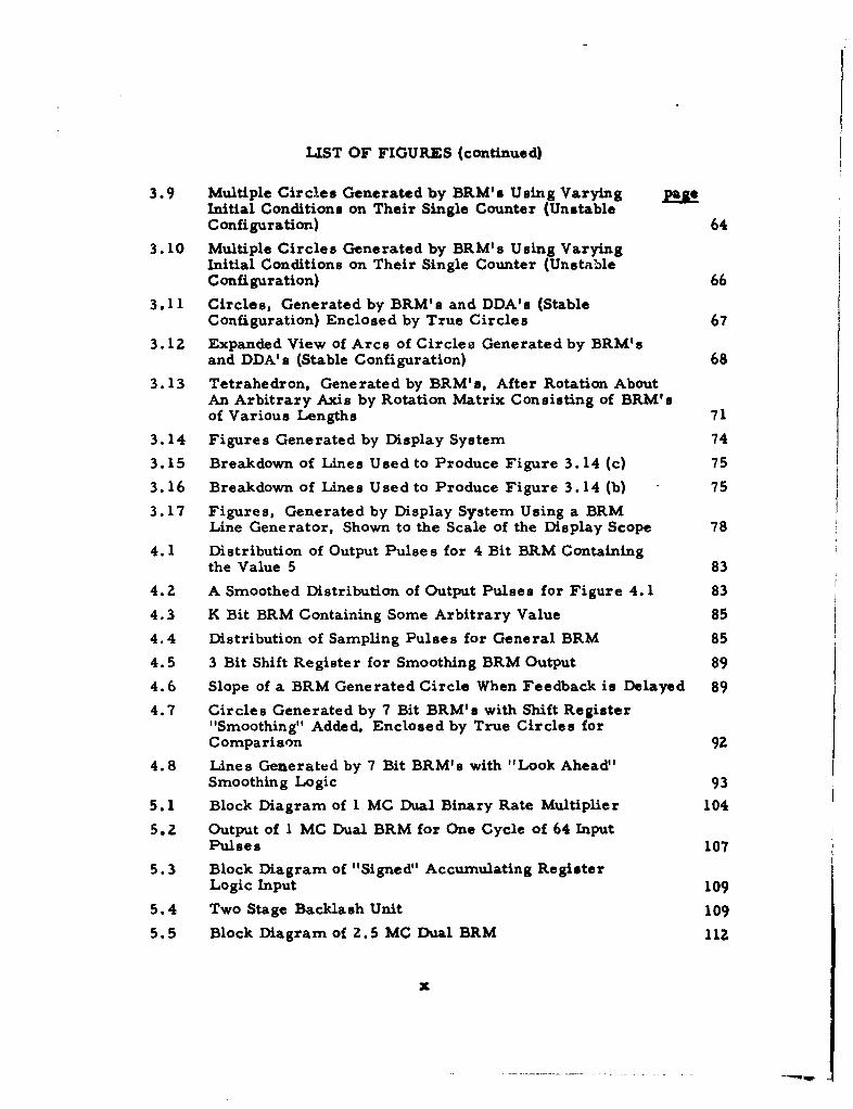
LIST OF FIGURES (continued)
5.6 Output of 2.5 MC Single BRM for One Cycle of page64 Input Pulses 114
6.1 Stereoscopic Projection Geometry 118
6.2 Block Diagram of Stereoscopic Projection DisplaySystem 118
6.3 Stereoscopic Viewer Using Polarized Lenses 120
6.4 Stereoscopic Viewer Using a Single Mirror 120
6.5 Left and Right Images of Stereoscopic Projection 122
6.6 Expansion of Images of Stereoscopic Projections ofTetrahedrons 123
6.7 Perspective Projection Geometry 125
6.8 Block Diagram of Perspective Projection DisplaySystem 125
6.9 Perspective Projection of a Block With a Hole ThroughIt, Generated by BRM's 127
A. 1 Simulation Program: Loop 1 140
A. 2 Simulation Program: Loop 2 140
A. 3 Simulation Program: Loop 3 141
A. 4 Simulation Program: Rotation Matrix 142
B. 1 Analog Display System 146
B. 2 Analog Sine-Cosine Generator 148
B. 3 Simplified Analog Display System 148
xi

e
CHAPTER I
THE COMPUTER DISPLAY PROBLEM
A. BACKGROUND
One of the deficiencies of digital computers of today is lack of really
satisfactory communication with the human operator. To make computers
more conversant with man, new and powerful computer languages such as
FORTRAN, ALGOL and COBOL have been and are still being developed.
But there are many concepts which are not easily expressed as relations of
numbers, or words, and therefore fall outside the scope of these languages.
One of the forms of human expression which is just now being exploited
for man-computer communications is that of graphic art. If a picture is
truly "worth a thousand words" it has great untapped potential. The
Computer-Aided Design Group of the Electronic Systems Laboratory
at M.I.T. is concerning itself with this potential as it applies to the design
of mechanical parts by a man with the direct aid of a digital computer. From
study done so far it has become evident that pictorial representation is an
extremely rapid and concise way to describe a shaped object to a computer.
A number of devices have been considered for the medium of this
graphical language but the most satisfactory has been the computer-controlled
cathode ray tube or "Display Scope". These scopes are becoming more
commonplace in computer installations, but are still not "standard equip-
ment". In all but a few notable exceptions these are point-for-point
plotting machines. (That is, in a single instruction the computer specifies
i -1-
,_ _ _ _ _ _ _ I_ _ _ _ _ __I_ __II
-a-
by its x and y coordinates a solitary point to be intensified oan the scope
face.) In the IBM 780 Display Unit there are 210 = 1024 possible x values
and as many y values. Thus there are over one million discrete points that
can be specified for display. This in essence constitutes the writing paper.
For a drawing implement a Light-Pen is used which is a tubular
device about the size and shape of a thick fountain pen with a photo cell
mounted at one end and a wire to the computer at the other. Through
proper display of points and sensing if the pen "saw" the points, the
computer can continuously determine and record the location of the pen
on the scope face, thereby tracking and storing what the operator has
drawn on the scope. The light-pen and the pen tracking operation are
described in detail in reference 1. In addition to the light-pen, special
buttons, dials, switches, and on-line typewriters are envisioned as
part of the man-machine console necessary for a truly versatile graphical
language facility.
Studies of graphical communications are being performed at M.I.T.
both at the Electronic Systems Laboratory and at the Lincoln Laboratory,
where Ivan Sutherland has prepared his "Sketchpad" system.2 Sutherland's
work has been done on Lincoln's ultra-high-speed TX-2 computer, while
Electronic Systems Laboratory has been workin6 on an IBM 709. In both
cases the light-pen is used to input a pictorial representation of the part.
The computer stores the pertinent information from this input and generates
Superscripts refer to numbered items in the Bibliography.
-3-
its version of the picture from this stored data. The display is con-
tinuously regenerated for the operator to view, even while pen tracking
is occurring.
B. THE PROBLEM
From the work done so far in displays on the 709 and TX-2, it has
become evident that an inordinately large amount of computer time is being
spent in the mundane job of generating the display. In this work the computer
stores the data, perhaps for a large three dimensional line drawing, in a list
structure of some sort. The display is generally the projection of a sub-
section of this large picture, which can be varied in size and position,
analogous to looking through a window at a large room. By moving the
room back from the window a larger section is seen in less detail. Trans-
lating the room with respect to the window brings in new portions to view.
Rotating the room changes the orientations of the objects seen through the
window. On the present point-plotting display systems available on the 709
and TX-2 computers, the computer program generates the picture by
forming a display file. This is a list of the points to be plotted, specified
in the scope horizontal and vertical coordinates. To produce the list,
first the window size, translation, and rotation are computed. Lines
or portions thereof which lie outside the region of display are eliminated.
Then a point-for-point listing is made of the remainder.
Once this display file is formulated, the data must be transmitted to
the scope, point-by-point, often enough to avoid flicker. This continues
until the operator calls for a change in the picture. Any change at all
means generation of a complete new list. Estimates by Sutherland for
his TX-2 programs are that of the time spent on generation of the display
-4-
list about 10% is spent on orienting the window to the total picture,
about 10% on deciding which parts of the picture are within the view of
this window, and 80% generating the point list.
On the ultra-high-speed TX-2 computer, a program exists which
generates a simple perspective picture, rotating it continuously but with
a high flicker rate. More complicated pictures get progressively worse.
G. Randa3 suggests several seconds would be required on an IBM 709 for
each view of an object being rotated. This is partly because the archaic
IBM 780 Display unit requires 140 microseconds to plot a single point.
Just displaying a 5, 000 point list (ten 5-inch lines) would require 0.7
seconds, not to mention the several seconds needed to generate the list.
Thus for even the most modest pictures, continuous CRT display by
computer is expensive and slow, occupying the lion's share of the computer
time. For the information rates being dealt with a more adequate tool is
required.
C. EXISTING CRT IMPROVEMENTS
Fortunately there are CRT systems in existence which contain significant
improvements over the point-for-point display units. Two devices in
particular which enhance CRT performance are a vector generator and a
character generator.
The vector generator is a unit which draws straight lines on the scope
face on command from the computer. The starting point of the line is the
last point previously plotted. The end point is specified by the computer.
The vector is swept out at a constant speed so the intensity is even over
the length of the line. Inclusion of a vector generator in a display system
permits a picture to be made up of a series of one-computer-word vectors
instead of a protracted point-for-point list, thereby reducing the list size

-5-
drastically and saving large amounts of computation time. Vectors can
also be plotted at rates nearly as fast as points, thus improving the
display rate by two orders of magnitude. The time spent generating the
vector list is similarly reduced.
The character generator produces special symbols, such as the
alphabet or the numerals, for display on the scope. It accepts 6 to 8 bit
binary codes as input and generates the necessary horizontal and vertical
deflection voltages to sweep out the shape of the decoded symbol in times as
short as a few microseconds. The sweep voltage outputs may be in
discrete steps or continuous in nature and are usually very rapid, often
requiring special deflection coils on the tube. The gross positioning of
the character on the tube face is usually done by separate circuitry,
independent of the character generator.
Use of a scope system which includes these improvements reduces the
display problem immensely and makes continuous display a feasible and
attractive facility.
Consider a display system containing a character and vector generator.
Assuming an improvement by a factor of 100 over the present 709 plotting speeds,
a picture consisting of straight-line vectors and text covering 5% of the
possible plotted points on the scope face could be maintained at a frame rate
of 15 frames per second.
With the display unit connected through the Data Synchronizer on the
709, one memory cycle (12 microseconds) would be "snatched" for each
vector (about every 100 microseconds for 1-inch vectors) and there would
occur only a 12%16 slow down of computer operation while maintaining full
display. However if the designer at the scope desires a continually
rotating picture, the display list must be regenerated each pass and this
causes grave problems.
-6-
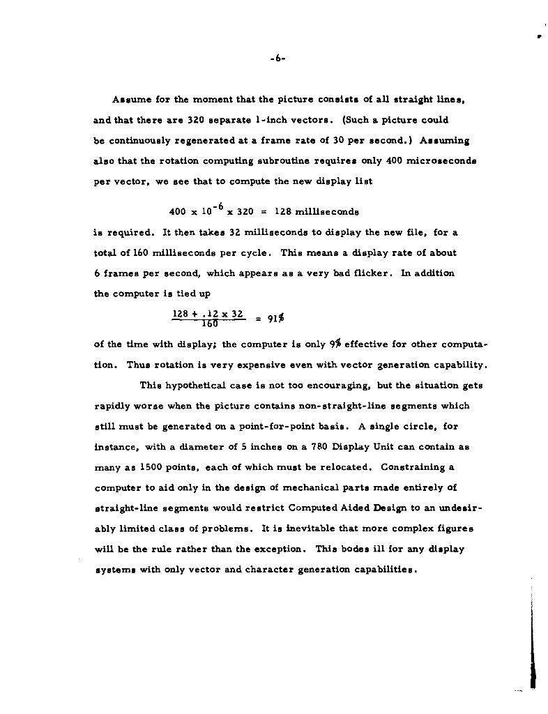
Assume for the moment that the picture consists of all straight lines,
and that there are 320 separate 1-inch vectors. (Such a picture could
be continuously regenerated at a frame rate of 30 per second.) Assuming
also that the rotation computing subroutine requires only 400 microseconds
per vector, we see that to compute the new display list
400 x 10-6 x 320 = 128 milliseconds
is required. It then takes 32 milliseconds to display the new file, for a
total of 160 milliseconds per cycle. This means a display rate of about
6 frames per second, which appears as a very bad flicker. In addition
the computer is tied up
128+ .12x32 = 91%160
of the time with display; the computer is only 9% effective for other computa-
tion. Thus rotation is very expensive even with vector generation capability.
This hypothetical case is not too encouraging, but the situation gets
rapidly worse when the picture contains non-straight-line segments which
still must be generated on a point-for-point basis. A single circle, for
instance, with a diameter of 5 inches on a 780 Display Unit can contain as
many as 1500 points, each of which must be relocated. Constraining a
computer to aid only in the design of mechanical parts made entirely of
straight-line segments would restrict Computed Aided Design to an undesir-
ably limited class of problems. It is inevitable that more complex figures
will be the rule rather than the exception. This bodes ill for any display
systems with only vector and character generation capabilities.
-7-
D. FUNDAMENTALS OF A SOLUTION
Two fundamental problem areas evidence themselves from the previous
discussion. The first is the large volume of data which must be continuously
fed to the scope. The second is the extensive computation required to generate
that data in meaningful form for the scope.
The solution proposed in this thesis to both these problems is to
build the necessary computing power into the display unit itself. In the
first case, it is absolutely essential in order to speed up the display to a
point where something other than non-trival pictures can be maintained.
In the second, it is economically advantageous in terms of both computer
time and programming time.
The computational capability required to speed up the display is
supplied by character, vector, and curve generation. The computer should
only be required to call out the parameters of a line and let the display
system produce the appropriate points that make up the drawing. The
display system should produce the necessary voltages to sweep out this
line at maximum speed. For a small number of often-used special-purpose
symbols (such as the alphabet and numerals) a character generator is useful,
while for straight lines a vector generator is needed. Curved lines can
become extremely complex so a compromise must be made. Fortunately
the human eye is very inexpert in distinguishing complex curves from
segments of simpler curves. For this reason, capacity for producing
second-order curves should suffice for all but the pathological cases.
The intelligence of the display system regarding the second problem,
(reducing the central processor load in generating the meaningful data)

-8-
is grossly subject to engineering compromise, since proper tradeoffs
between hardware complexity and computer and programmer time are
vague and illusory If the display system is made sophisticated and
powerful, it can handle the display virtually independent of the computer.
This however become s expensive. A less intelligent machine might be
built which would take some of the load off the main frame but not be
independent of it. The least sophisticated display system which would
still be considered acceptable would be that minimal machine which fulfills
the dictates of the first problem, display speed. In essence this would
do none of the computation of reducing the three-dimensional picture to a
projection in two dimensions. Lines* would be specified in two-dimensional
scope coordinates only.
The system which is discussed in the remainder of this thesis is one
which is somewhere betweenthe minimal machine and the expensive
sophisticated one. It contains the hardware required to generate straight
lines, second-order curves, and characters. It also performs the
necessary computations to transform the picture from three-dimensional
coordinates to the rotated two-dimensional scope coordinates, based only
on a minimal set of parameters from the computer. As such it falls
into the catagory of a "special purpose computer", or more appropriately
perhaps "specialized computing equipment".
In this system the outputs from the computer to the display are the
scope coordinate system parameters, plus the component parts of the
picture to be shown. The component parts are the lines making up
Throughout this thesis "lines" refers to curved as well as straight lines,except when context clearly indicates otherwise.
"-9-
the object. Since the figures being dealt with are principally three-
dimensional, these lines must be specified in three dimensions.
The scope coordinate parameters are those numbers which delineate
the scope coordinates relative to an absolute coordinate system in which
the picture is stored in computer memory. In our earlier analogy, they
describe the position and size of the window with respect to the room.
The parameters required for an axonometric projection are the rotation
matrix to specify the orientation, the starting position to specify
the translation, and a magnification factor. A perspective or stereoscopic
projection would require more parameters.
E. A SYSTEM SOLUTION
The system desired is one which will provide a rotated axonometric
projection on a scope of a subsection of a three-dimensional line drawing
stored in a computer. The system must be capable of generating first
and second-order lines from computer commands. It should provide
easy means for the computer to translate or rotate the picture, or to
magnify or demagnify it. If possible, some way for preventing plotting
when the limits of the scope edge are reached should be incorporated,
whether it be under computer control or self-contained in the display
unit.
More complicated projections such as perspective or steroscopic
views might be desirable but are more difficult to generate. A later chapter
discusses the system required to produce these projections. For the present
we shall concern ourselves only with the simpler axonometric system.
Figure 1. 1 illustrates a realization of the desired system. It is
made up of three main parts. The first part is the line generating unit,
-10-
I ] I
0 II
x@I -~I Nd
it
U>
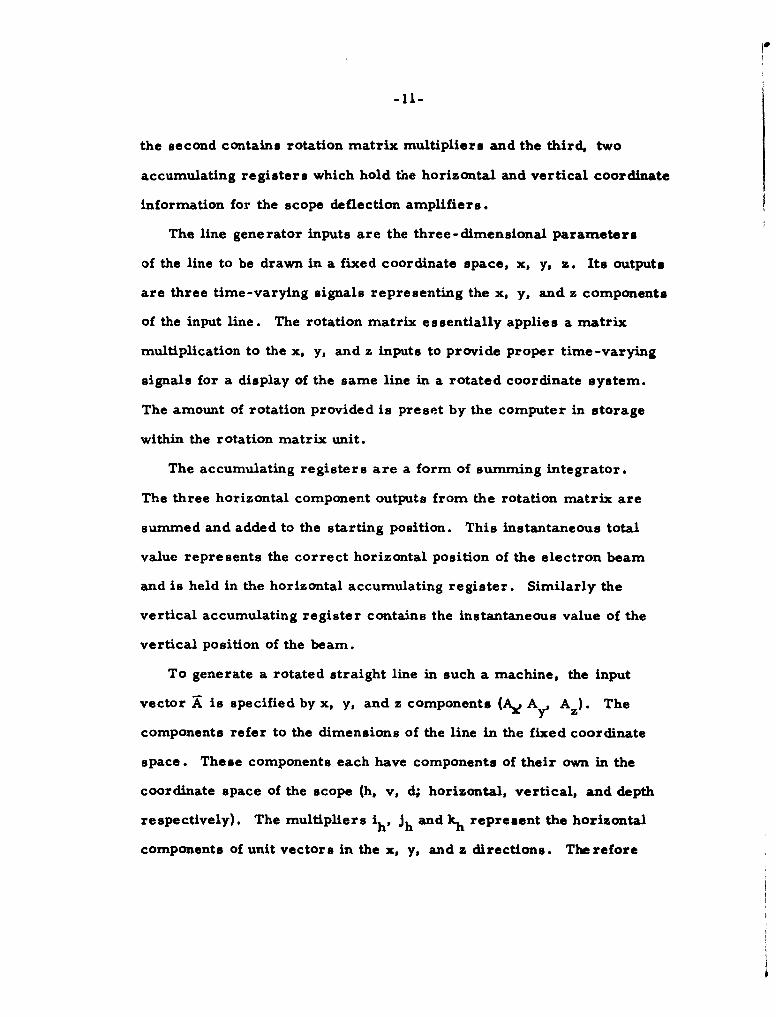
the second contains rotation matrix multipliers and the third, two
accumulating registers which hold the horizontal and vertical coordinate
information for the scope deflection amplifiers.
The line generator inputs are the three-dimensional parameters
of the line to be drawn in a fixed coordinate space, x, y, z. Its outputs
are three time-varying signals representing the x, y, and z components
of the input line. The rotation matrix essentially applies a matrix
multiplication to the x, y, and z inputs to provide proper time-varying
signals for a display of the same line in a rotated coordinate system.
The amount of rotation provided is preset by the computer in storage
within the rotation matrix unit.
The accumulating registers are a form of summing integrator.
The three horizontal component outputs from the rotation matrix are
summed and added to the starting position. This instantaneous total
value represents the correct horizontal position of the electron beam
and is held in the horizontal accumulating register. Similarly the
vertical accumulating register contains the instantaneous value of the
vertical position of the beam.
To generate a rotated straight line in such a machine, the input
vector X is specified by x, y, and z components (Ae Ay, Az). The
components refer to the dimensions of the line in the fixed coordinate
space. These components each have components of their own in the
coordinate space of the scope (h, v, d; horizontal, vertical, and depth
respectively). The multipliers 'h, Jh and kh represent the horizontal
components of unit vectors in the x, y, and z directions. Therefore
-12-
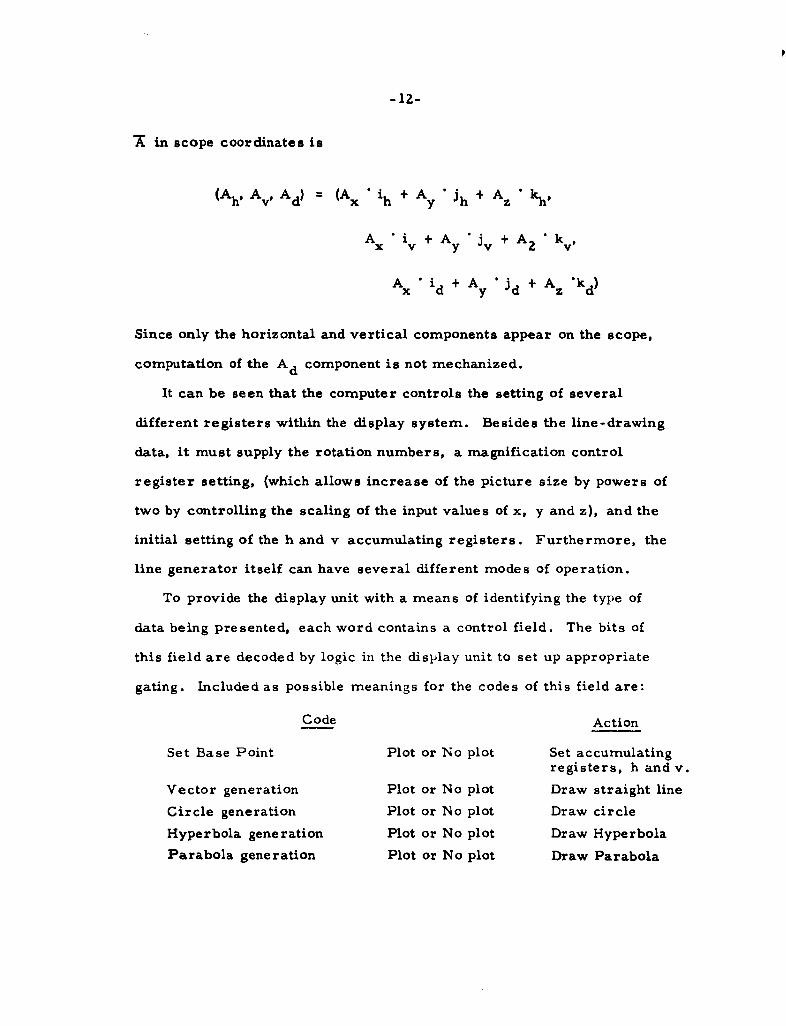
X in scope coordinates is
(Ah, AV, Ad) (Ax " ih + Ay ' Jh + Az * kh,
Ax "iv + Ay * jv + A2 " kv'
Ax * id + Ay 'Jd + Az "kd)
Since only the horizontal and vertical components appear on the scope,
computation of the Ad component is not mechanized.
It can be seen that the computer controls the setting of several
different registers within the display system. Besides the line-drawing
data, it must supply the rotation numbers, a magnification control
register setting, (which allows increase of the picture size by powers of
two by controlling the scaling of the input values of x, y and z), and the
initial setting of the h and v accumulating registers. Furthermore, the
line generator itself can have several different modes of operation.
To provide the display unit with a means of identifying the type of
data being presented, each word contains a control field. The bits of
this field are decoded by logic in the display unit to set up appropriate
gating. Included as possible meanings for the codes of this field are:
Code Action
Set Base Point Plot or No plot Set accumulatingregisters, handv.
Vector generation Plot or No plot Draw straight line
Circle generation Plot or No plot Draw circle
Hyperbola generation Plot or No plot Draw HyperbolaParabola generation Plot or No plot Draw Parabola

-13-
Code Action
Set Mh(i'h Jh' kh) Set h components ofrotation matrix
Set M (iv, J kv) Set v components ofV vrotation matrix
Set magnification Set magnificationregister
Character generation Draw character
To produce a single homogenous picture with this system, the program
in the computer forms a sequential list of the lines to be drawn. In this
list each successive line begins where the last left off. Because of this
blank lines must often be included to reposition the beam for the
starting point of a new line. If the list is made up solely of interconnected
straight lines, a single setting of the rotation matrix values will suffice
to control the orientation of the view. If however base point deflection is
used to reposition the beam for starting points of new lines, rather than
blank vectors, the drawing is split into discrete parts, and when rotation
is done those newest starting points must be separately calculated by the
computer. A typical display file is shown below.
It
-14-
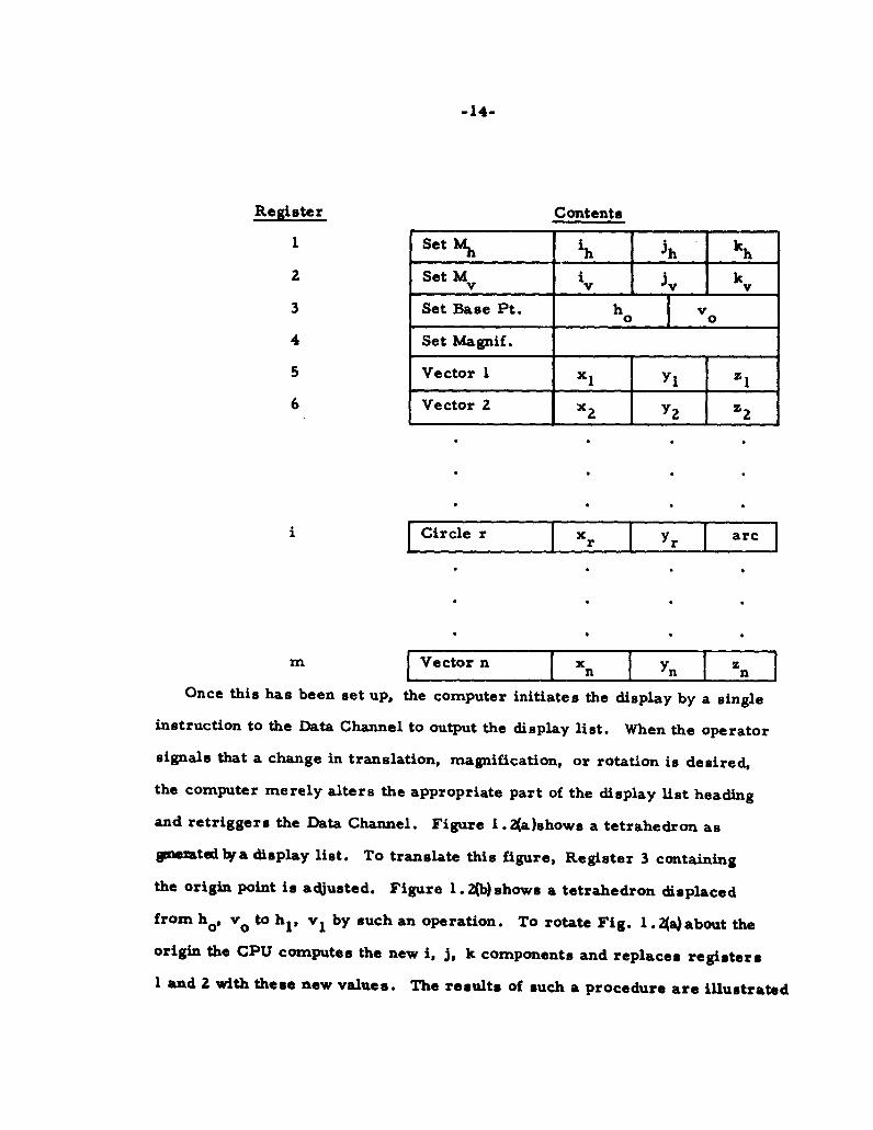
Register Contents
1 Set Mh ih 1 h kh
2 Set Mv iv Jiv kv
3 Set Base Pt. ho vo
4 Set Magnif.
5 Vector 1 1Xy Yl z6 Vector 2 x 2 Y2 z_2
i circle r Xr Yr arc
m Vector n x- yn zn
Once this has been set up, the computer initiates the display by a single
instruction to the Data Channel to output the display list. When the operator
signals that a change in translation, magnification, or rotation is desired,
the computer merely alters the appropriate part of the display list heading
and retriggers the Data Channel. Figure 1. 2(a)shows a tetrahedron as
SwexatedbIa display list. To translate this figure, Register 3 containing
the origin point is adjusted. Figure 1. 2(b) shows a tetrahedron displaced
from ho, v 0 to hI, vI by such an operation. To rotate Fig. 1 .2(a) about the
origin the CPU computes the new i, J, k components and replaces registers
1 and 2 with these new values. The results of such a procedure are illustrated

-15-
Vo Vo
ho ho h,
V0 - - 0 - ---- V
(a) (b)
V2
hoh h
(C) (d)
Fig.1-2 Examples of Translation and Rotation of a Figure by theDisplay System

-16-
in part (c)of Fig. 1. 2. Vector 1 is often made to be zero length so
that rotation about some point other than the present starting point may
be easily accomplished. This is done by specifying a new origin
(register 3) and loading register 5 with a "blank" vector which moves
the display back to the correct starting point for vector 2. If for
instance the tetrahedron of Fig. 1.2 a is to be rotated about the point
h 2 , v 2 instead of ho, vo, register 3 is set to h 2 , v 2 and register 5 is
changed fromx = 0, y = 0, z = 0 tox = hO-h 2 , y = vo - v2 , z = 0,
and the rotation matrix is set to affect the desired rotation. Magnification
can be handled by changing all the i, j, k components by an appropriate
factor, or by altering the magnification control register, or by a
suitable mixture of both.
A large portion of the computation load is relieved by this equipment,
but the central processor is still required to perform the time-consuming
chore of "edging". This is the task of calculating where a line runs off
the edge of the scope, and should therefore no longer be displayed. This
"edging" problem can be minimized by building the h and v registers so
that they can hold values larger than the maximum scope deflections. If
the computer tries to display lines which are off the edge of the scope,
special sensing logic can detect that h or v are greater than the scope
limits and cease further transfer to the scope deflection coils, as well
as preventing scope unblanking. The machine continues to process the
the transmitted data as though actual display was occurring. When
the lines work their way back into the limits of the scope, plotting takes
-17-
up again. The one disadvantage of this system of edging is that the
effective display rate is slowed, since the system is taking time to
process data that never appears on the scope. A compromise might be
for the display unit to set a sense line to the computer whenever the
display is off the viewing screen. If the display is overloaded so
that the slow-down causes flicker, the computer can test this sense
line and rewrite the list to eliminate the extraneous lines, or can return
to the procedure which is now used, computing the edges and completely
revamping the display list.
The strength of this display system lies in the fact that at all times
the computer maintains complete control over the display without being
forced to do the large amounts of trivial processing presently required
to produce the display. The program can easily set limits on the controls;
for example when the horizontal starting position reaches some arbitrary
bound, a new part of the over-all picture can be loaded in as the display
list. If a more sophisticated display is desired such as a perspective
projection, the computer can perform the three-dimension to two-
dimension transformation and use only the line drawing capabilities.
Or if desired, the computer can even return to point-for-point
calculations.
CHAPTER II
REALIZATIONS OF THE SYSTEM SOLUTION
A. INTRODUCTION
Two basic approaches were considered for manifesting a hardware design
of the proposed system; analog and digital, although not in that order. The
digital approach seemed favorable from a number of standpoints: expense,
reliability, engineering effort involved, and accuracy. Rather than take the
time to describe them at this juncture a brief discussion of two analog approaches
which were considered is given in Appendix B.
The digital approach is based on incremental computing techniques, using
either Binary Rate Multipliers or Digital Differential Analyzers. This
chapter describes these devices. The basic idea of the digital techniques
is that the horizontal and vertical components of the electron beam position
are changed in discrete steps with time. The time-varying signals from
the line generator are then trains of pulses whose rates specify numerical
information. The rotation matrix accepts the pulses as input and produces
its own pulse strings as output. The accumulating registers are then simple
up-down counters which count the pulses and continuously indicate the final
control variable.
The Binary Rate Multiplier and Digital Differential Analyzer are computing
devices which operate on pulse trains. They represent the candidates for
the building blocks of our display system. We shall begin our discussion with
a description of the Binary Rate Multiplier.
-19-

-20-
B. BINARY RATE MULTIPLIERS
1. Description
The Binary Rate Multiplier (BRM) is a digital device which performs
rate multiplication, i.e. for a given rate of pulses input, the BRM will
output a pulse rate which is a variable fraction of the input rate. For
a complete description of the BRM and an analysis of its errors the reader5
is referred to Haring. Basically a BRM consists of a data register, y, of
m binary bits, a counter register also of m bits, and pulsed "AND" gating
between the two registers, as illustrated in Fig. 2. 1.
In binary counting (illustrated in Table 2. 1) it will be noted that for
each pulse in, there are any number of I to 0 transitions (with subsequent
carry to the next stage) in the elements of the counter, but only a sinigle
0 to I transition (where the carry stops). If the data register contains a
I at the corresponding position, an output pulse occurs. The least significant
counter digit makes the 0 to 1 transitions, evenly spaced over the Zm counts,
at a frequency of f/2, where f is the input clock frequency. The second
least significant digit of the counter makes f/4 transitions, likewise evenly
spread over the Zm counts, and so it goes through all m digits, the last
making a single 0 to 1 transition. Therefore the l's in the data register
will select a combination of frequencies, f/ 2 k, which are summed by the
output OR gate. If the contents of the data register is treated as an m-bit
binary fraction, r, the output rate is precisely rfo. Hence the name binary
rate multiplier.

BINARY COUNTERI
2~- LEVEL1
PLSES2L - - - COUNTER -EGISTER
Fig.~~~~~~ 2. h.BtBR otiig h au

Table 2. 1
Counter bit Decimal 0 to 1a b c d Count Transition
0 0 0 0 0
1 0 0 0 1 a
0 1 0 0 2 b
I 1 0 0 3 a
0 0 1 0 4 c
1 0 1 0 5 a
0 1 1 0 6 b
1 I 1 0 7 a
0 0 0 1 8 d
1 0 0 1 9 a
0 1 0 1 10 b
1 1 0 1 11 a
0 0 1 1 12 C
1 0 1 1 13 a
0 1 1 1 14 b
1 1 1 1 15 a
0 0 0 0 0
An alternate way to consider the BRM is to treat the contents of the data
register as a fixed binary integer, with the most significant bit in al, next
most significant in a 2 , etc. If this number remains fixed throughout 2 m
input pulses then the number of output pulses through the OR gate in Fig. 2.1
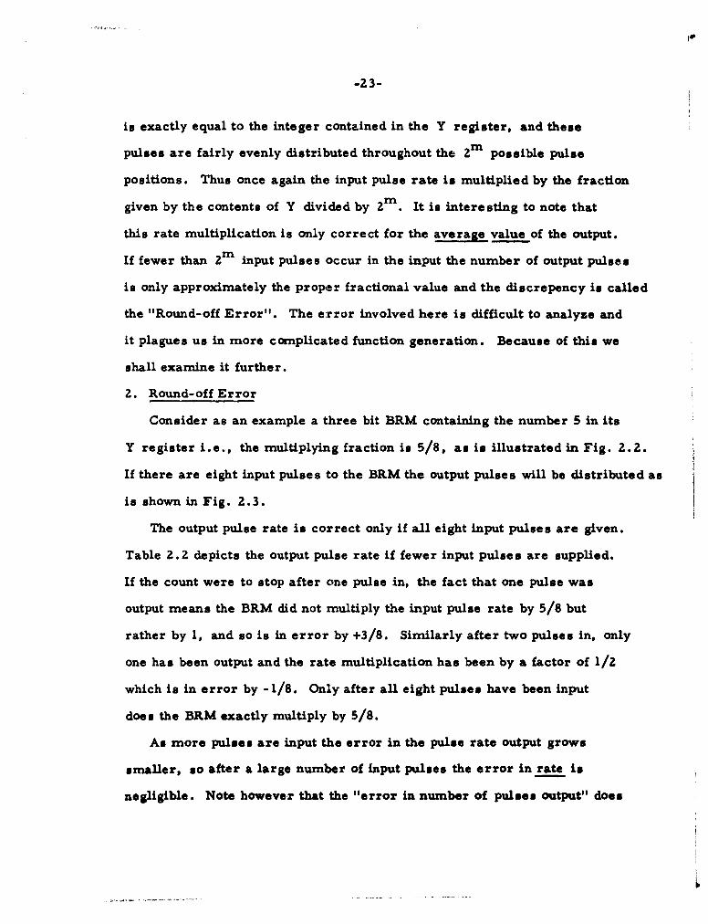
-23-
is exactly equal to the integer contained in the Y register, and these
pulses are fairly evenly distributed throughout the 2 m possible pulse
positions. Thus once again the input pulse rate is multiplied by the fraction
given by the contents of Y divided by 2 m. It is interesting to note that
this rate multiplication is only correct for the average value of the output.
If fewer than 2m input pulses occur in the input the number of output pulses
is only approximately the proper fractional value and the discrepency is called
the "Round-off Error". The error involved here is difficult to analyze and
it plagues us in more complicated function generation. Because of this we
shall examine it further.
2. Round-off Error
Consider as an example a three bit BRM containing the number 5 in its
Y register i.e., the multiplying fraction is 5/8, as is illustrated in Fig. 2.2.
If there are eight input pulses to the BRM the output pulses will be distributed as
is shown in Fig. 2.3.
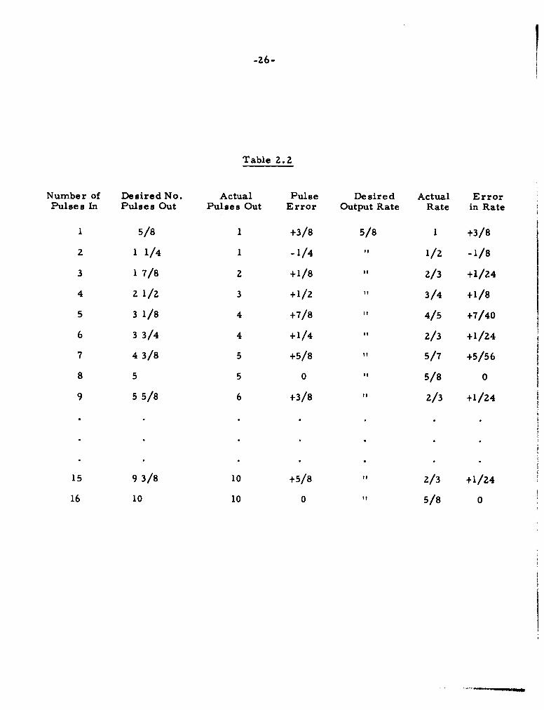
The output pulse rate is correct only if all eight input pulses are given.
Table 2.2 depicts the output pulse rate if fewer input pulses are supplied.
If the count were to stop after one pulse in, the fact that one pulse was
output means the BRM did not multiply the input pulse rate by 5/8 but
rather by 1, and so is in error by +3/8. Similarly after two pulses in, only
one has been output and the rate multiplication has been by a factor of 1/2
which is in error by -1/8. Only after all eight pulses have been input
does the BRM exactly multiply by 5/8.
As more pulses are input the error in the pulse rate output grows
smaller, so after a large number of input pulses the error in rate is
negligible. Note however that the "error in number of pulses output" does

"-24-
INPUT i tIPULSES _ ~
1 2 3 4 5 6 7 8
OUTPUT
f f f 1 f22 S 2 2-
COUNTERSTATE 100 010 110 001 101 OI II I 000
DATA BIT a b a c a b a noneSAMPLED
Fig.2-3 Distribution of Output Pulses from BRM of F1g.2-2
VVU
i- 4 Pio COUNTER
DELAY I
xiaxi_, +Vxi {+
F19.2-4 BRM Pair to produce Sine-Cosine

-25-
not diminish, since one can not output a fraction of a pulse. This
"error in pulses output" is called the round-off error, although this
is somewhat of a misnomer when the value in the data register is
variable, since the error is a dynamic one. As pointed out by Haring, these
errors are extremely difficult to predict. We shall see the difficulties caused
by these errors in Chapter IMl.
3. The General Binary Rate Multiplier
In using BRM's for general computation numerical values are represented
by pulse rates. In order to compute with positive and negative numbers, it
is necessary to associate with each rate a "sign" and make the "sign" of
the BRM output the logical product of the "sign" of the input pulse rate and the
data register. This sign information is used to control whether an accumulating
register is incremented or decremented by the output pulse train.
In this study we will also use BRM's with unidirectional counters as
described in the preceding section. A more accurate scheme would be to
make the counter of the BRM reversible. That is it should be capable of
counting down as well as up, in accordance with the "sign" of the input
pulse train, and produce output of appropriate "sign". This would require
additional logic to produce output pulses when counting down, since in this
operation it is the 1 to 0 transitions which are significant. Under this
arrangement negative input pulses cause the counter to cycle backwards
through exactly the same states it passed through during previous positive
input pulses. However since the distribution of I to 0 transitions in
decrementing logic is the same as 0 to I transitions in incrementing logic,
-26-
Table 2.2
Number of Desired No. Actual Pulse Desired Actual ErrorPulses In Pulses Out Pulses Out Error Output Rate Rate in Rate
1 5/8 1 +3/8 5/8 1 +3/8
2 1 1/4 1 -1/4 " 1/2 -1/8
3 1 7/8 2 +1/8 " 2/3 +1/24
4 2 1/2 3 +1/2 it 3/4 +1/8
5 3 1/8 4 +7/8 of 4/5 +7/40
6 3 3/4 4 +1/4 It 2/3 +1/247 4 3/8 5 +5/8 5/7 +5/56
8 5 5 0 " 5/8 0
9 5 5/8 6 +3/8 2/3 +1/24
15 9 3/8 10 +5/8 2/3 +1/24
16 10 10 0 5/8 0

-27-
the average output is the same if a unidirectional counter is used and
the negative inputs are handled the same as positive inputs. In this
case a "truncation" error is introduced each time the sign of the input
changes, but this error is small and occurs infrequently and therefore
does not warrant the added logic.
To make the BRM more flexible, binary scale factors are often
applied to the BRM output. Thus the output of one BRM can be weighted
more heavily than the output of a second BRM. In the analysis used in
this thesis all outputs are weighted the same amount so this scaling can
be neglected.
C. LINE GENERATION
1. Vector Generation
Vector generation can be accomplished by storing x, y and z components
in thiee separate BRM's and then running them simultaneously from the
same clock source. The pulse rates from the BRM's will be proportional
to the vector components. Rotation can be accomplished by multiplying these
rates by terms of a rotation matrix stored in six i, j, k registers, each of
which is another BRM. The outputs of the ih, Jh' kh BRM's must then be
summed and added into the horizontal accumulating register, while a similar
operation is occurring with the vertical components.
If the data register of a BRM is also made to be a counter and the
outputs of some BRM's are connected as inputs to others, more complex
functions than straight lines can be generated. In particular, second order
curves can be formed by a pair of BRM's.

-28-
2. Circle Generation
Consider a BRM pair which is connected as shown in Fig. 2.4. In this
figure and in the remainder of this report:
i = number of the input pulse i.e. iteration count
VXi = Xi - Xi-1, the change in Xi from iteration i-I to i.
X. = the value of the variable x at iteration i.
Vt = independent variable input pulse rate. i.e. clock pulses
WV, VU = output pulse rates.
The data registers are bi-directional counters and contain the magnitudes of
the two variables x and y. Vt is the input clock. Vt' is delayed from Vt
enough to allow the output of the Y BRM (caused by Vti) to alter X before
Vt'. occurs to trigger the X BRM.
To make this analytically tractable we must first assume that each BRM
is an ideal rectangular integrator, i.e. the output rate is precisely the
correct fractional value of the input rate (which we noted in Table 2.2 is not
quite true).
ThenVU. = Y.h = VX.1 11
VVi = Xih = VY i+
where h is the fractional value of the least significant bit of the BRM
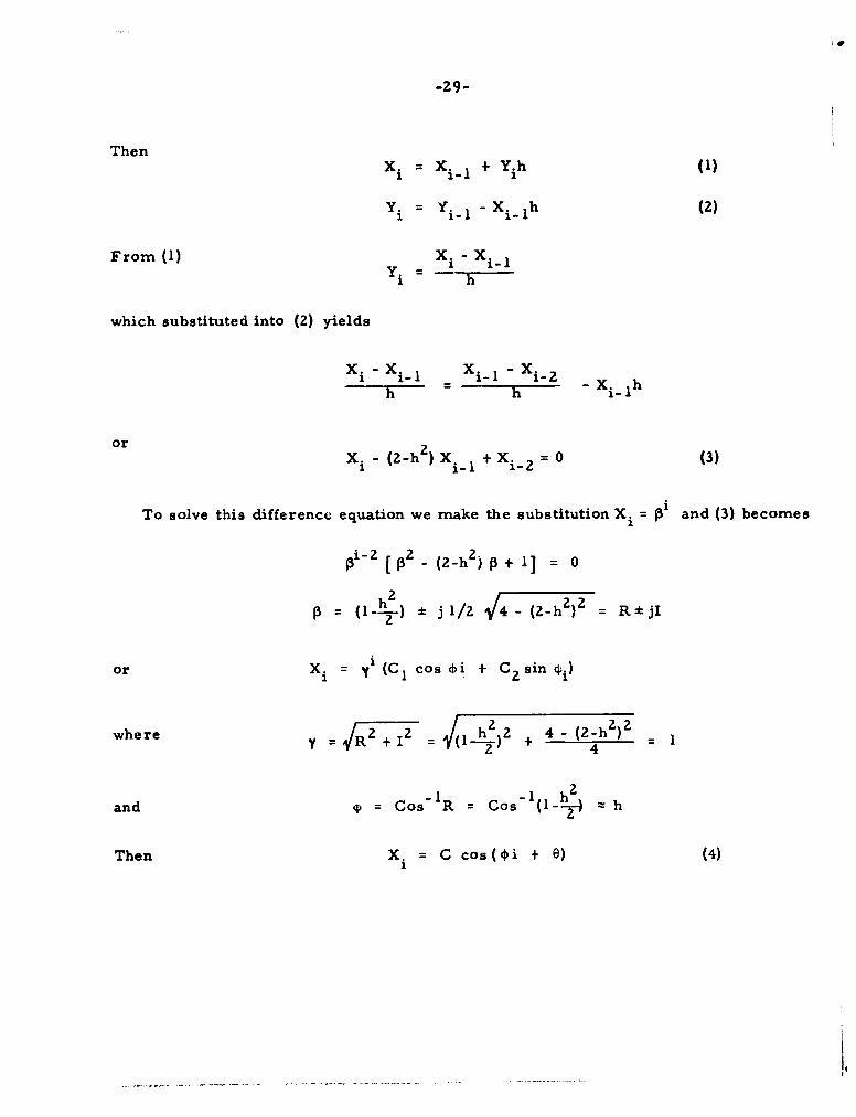
-29-
ThenX X 1 + Yih (h)
Yi Yi- - x i- h (2)
From (1) X -Xy. - -
which substituted into (2) yields
X i - i-I Xi- Xi- x h
or X - (2-h2) Xi_1 + Xi-z = 0 (3)
To solve this difference equation we make the substitution X. = •i and (3) becomes
• i - 2 [ P ? _ ( .h ?) P + 1 0h 2
(1- [2 -(2h/? l V( 02h) =R
or X. = 1 (C1 cos dci + C 2 sin i)
where ýR 2 +1 2 4h2 ) 2 + 4-(2-h2 )
and = Cos- R = Cos (1--) = h
Then X = C cos(li + O) (4)1
-30-
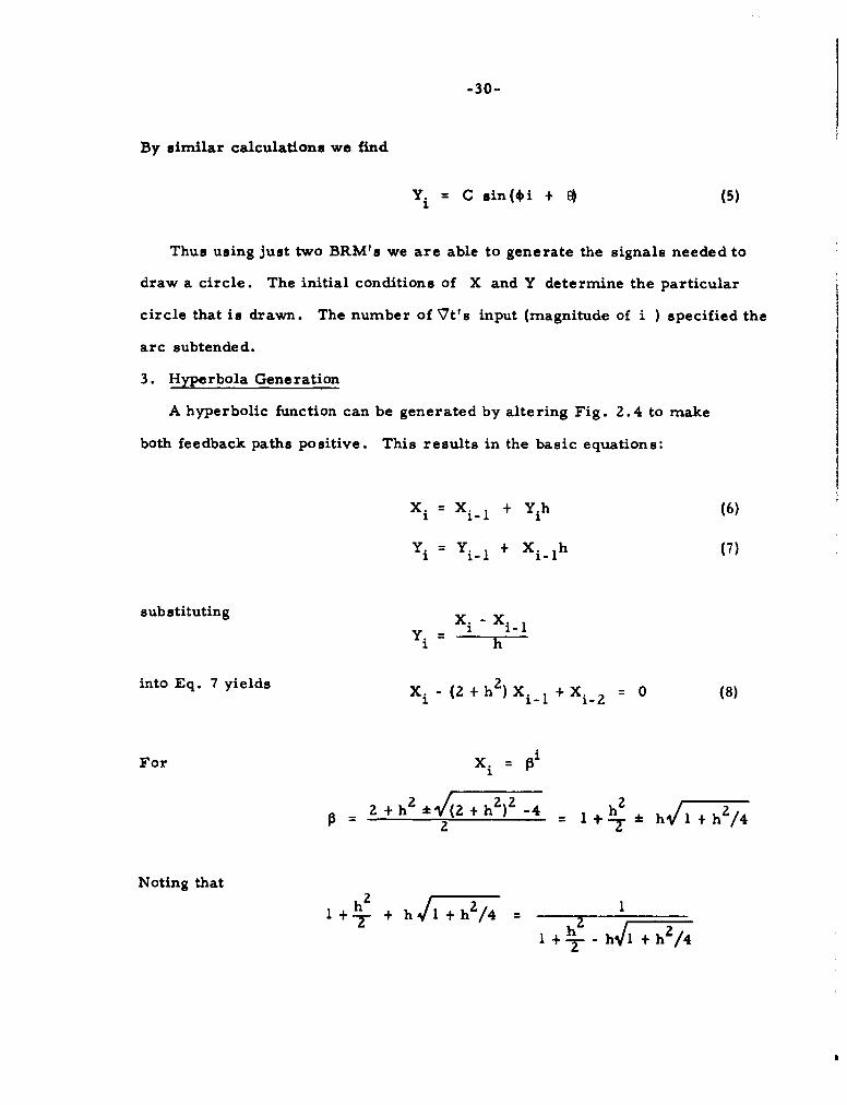
By similar calculations we find
Yi = C sin(*i + 8) (5)
Thus using just two BRM's we are able to generate the signals needed to
draw a circle. The initial conditions of X and Y determine the particular
circle that is drawn. The number of Vt's input (magnitude of i ) specified the
arc subtended.
3. Hyperbola Generation
A hyperbolic function can be generated by altering Fig. 2.4 to make
both feedback paths positive. This results in the basic equations:
X =XiI + Yih (6)
Y = Yi-I + X i-I h (7)
substituting X -X
i h
into Eq. 7 yields xi - (2 + h 2 Xi_1 +Xi-2 0 (8)
For Xi = •i
2 + h2+ -4 + hh/2 -T*h=l+h/
Noting that
h 2 h T 7 1I+T + h/l + h 2 /4 h
I+ h41 + h2/4

-31-
we can write our solution as
Xi= C1(e') + C2 (e'2)1 + C', sinh (ai) + C. cosh (ai) (9)
=L hz ZZ]where e 1 + +--hJl + h2/4 = [• + h2/2]2
and a= 2 loge [h +V + (h/2)i2-] = 2 sinh-l(h/Z) zh
for small h.
Solving for Yi we obtain a similar solution and thus meet the requirements
for hyperbola generation.
4. Parabola Generation
The basic equation of a parabola is
2y = ax
or in terms of incremental computation
Y = aX X (10)
1 1
Considering for the moment that a = 1, this means that
2 X221Y X - X 1 " (Xi - VXi)2
VYi = XI VXi - VX = XiVXi + (Xi -VXi) VXi
Vyi Xi i'x + Xi. 1 Xi (1)
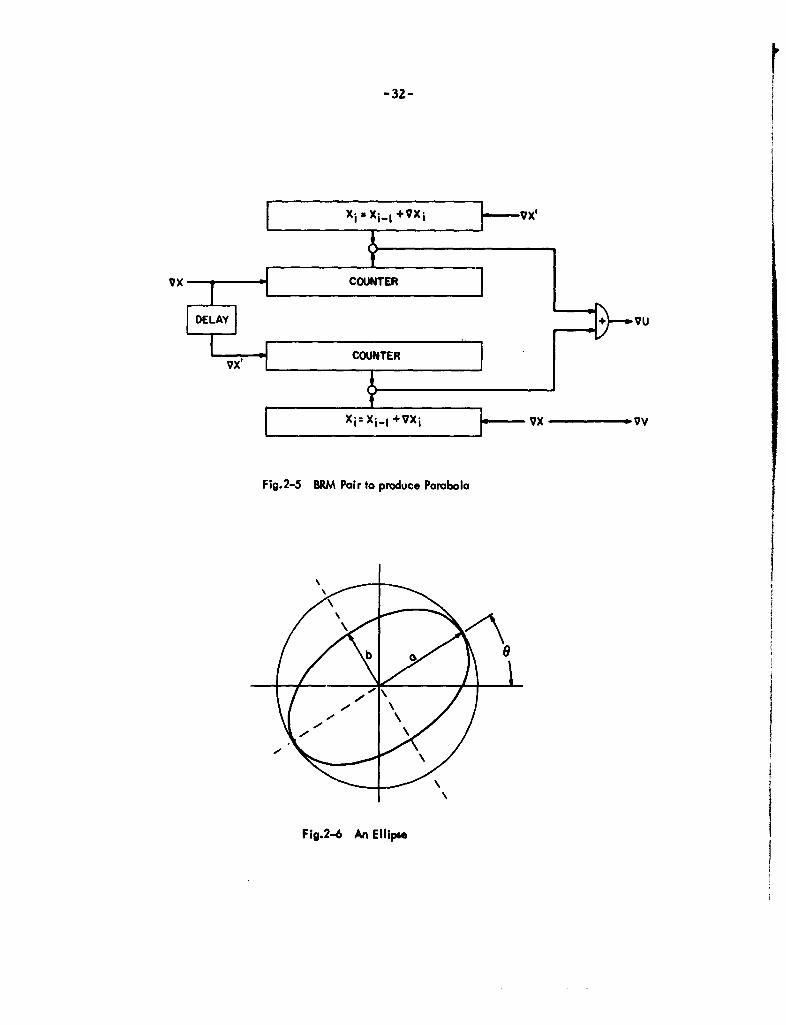
-32-
[ ~ ~~Xi a Xi-i +qXi •--X
DELAY + VU
VX' •COUNTER
vx'
F - ximxi-I +Vxi vx v
Fig.2-5 BRM Pair to produce Parabola
Fig.2-6 An Ellipse
-33-
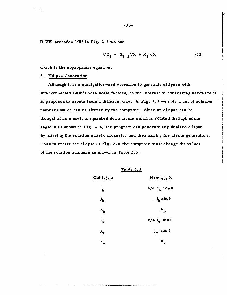
If VX precedes VX' in Fig. 2.5 we see
VU = X 1 VX + X VX (12)
which is the appropriate equation.
5. Ellipse Generation
Although it is a straightforward operation to generate ellipses with
interconnected BRM's with scale factors, in the interest of conserving hardware it
is proposed to create them a different way. In Fig. 1. 1 we note a set of rotation
numbers which can be altered by the computer. Since an ellipse can be
thought of as merely a squashed down circle which is rotated through some
angle 0 as shown in Fig. 2.6, the program can generate any desired ellipse
by altering the rotation matrix properly, and then calling for circle generation.
Thus to create the ellipse of Fig. 2.6 the computer must change the values
of the rotation numbers as shown in Table 2.3.
Table 2.3
Old i, j,k New i,j,k
ih b/a ih cos e
Jh "Jh sin e
kh kh
I b/a i sineiv v
iv Jv cos e
k kv v
-34-
Since the initial conditions on the circle are controllable by program,
any segment of this ellipse may be generated.
In a similar manner, any generalized parabola or hyperbola or segment
thereof can be created. That is the parabola produced by the line generator
of Fig. 1.1 is always the one described by the equation y = x . By
suitable presetting of the i, j, k numbers, any desired variation can be
drawn. In the same way the hyperbola generated is always one with an
eccentricity = 2. The rotation matrix is altered to give any other eccentricity.
D. THE BRM LINE GENERATOR
Thus we see that the line generator of Fig. 1. 1, capable of producing
straight lire s and conic sections, can be built with just three BRM's with
suitable control logic for interconnecting inputs and outputs. This configuration
however relies upon the presence of a rotation matrix following the line generator
to produce any generalized second order curve. A price is paid for this
simplicity in that the display list described in Chapter I is now broken up by
resettings of the rotation matrix each time a different curve is drawn. Thus
whenever a connected picture is to be rotated the computer must not only alter
the heading of the display list, but it must also recompute each of these matrix
settings. This computation is extremely simple consisting of a single matrix
multiplication. In the light of the simplicity to the hardware it permits, this
restriction on the display list seems justified.
E. ACCUMULATING REGISTERS
The final operation to consider is the accumulation of the matrix BRM
outputs with h and v registers. Since their outputs are pulse trains, it
is entirely feasible to perform this accumulation with simple counters. Since

-35-
it is possible for as many as three rotation matrix outputs destined for
the same accumulator to occur on the sarne clock pulse, it is important
to resynchronize these outputs to the basic clock and add appropriate
delays to stagger the accumulator inputs in time.
Figure 2.7 is a block diagram of the system using the Binary Rate
Multiplier as the basic unit. The diagram does not attempt to show all
the information flow paths such as the direct loading of the Rotation
Matrix values or the Accumulating Registers, but does indicate the
resynchronizing delays.
F. DDA SYSTEM
1. DDA Description
A second digital display system is worth considering at this time. This
uses the Digital Differential Analyzer (DDA) as its basic building block .Ln
place of the BRM. The DDA is an incremental computing device which per-
forms the same operation as the BRM, but in a slightly different manner. Since
it requires the same inputs as the BRM and produces a similar output (a pulse
train at some fractional value of the input pulse rate) the system diagram of
Fig. 2.7 is the same for the DDA system except a DDA replaces each BRM.6
The DDA is described and analyzed very thoroughly by F. Hills to whom
the reader is referred. Briefly a DDA consists of two registers; a data register
D, a remainder register, R, and an adder circuit between the two as shown in
Fig. 2.8. The input pulses activate the adder which adds the contents of D to
R and stores the results in R. After several input pulses the capacity of R
will be exceeded and it will overflow. This overflow is the DDA output pulse
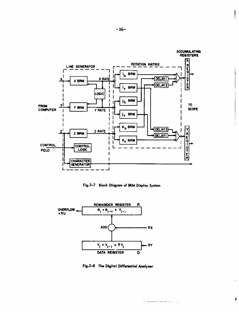
-36-
ACCUMULATINGREGISTERS
CONTROLENECOTOROLTTINIATI
xXREAINER REGISTE I
I J h-I
D ATA K REIT R M DEA 2
Z i.- The D[DEtal DifrnRlAaye

-37-
and corresponds to the BRM output pulse. Note that the rate of these output
pulses is directly proportional to the number in D, i.e. depending on the
size of D, varying numbers of input pulses are required to produce overflow.
The equations of a DDA are*
Yi = Yi-I +VYi (13)
VUi +Ri = Yi Ci +RiI (14)
where i again refers to an index on the number of input clock pulses, Y to
the value in the data register and R to the value in the remainder register.
Summing the output over n input VX's we obtain
n n nUn= VU - Y Yi - VRi
i=0 i=0 1=0
or n
Un= Z Y VXi-Rn +Ro (15)
i= 0
Thus the DDA approaches a perfect rectangular integrator except for the
value left in the R register, which is always less than one output pulse. The
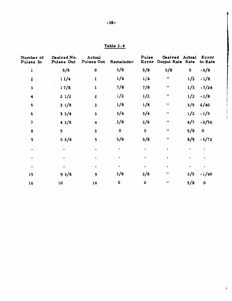
output is still, however, subject to this "round-off error". Table 2.4 shows the
output pulse distribution for a three bit DDA containing the number 5 starting with
the R register zeroed. It is interesting to compare this with Table 2.2 illustrating
the BRM distribution. The advantage of the DDA over the BRM is that at all times
it contains the amount of the round-off error in the R register and does not rely
on the round-off errors averaging out. This can best be illustrated by a
comparative example.
WHere as in the BRM equations scale factors are considered to be I.
-38-
Table 2.4
Number of Desired No. Actual Pulse Desired Actual Error
Pulses In Pulses Out Pulses Out Remainder Error Output Rate Rate in Rate
1 5/8 0 5/8 5/8 5/8 0 -5/8
2 11/4 1 1/4 1/4 to 1/2 -1/8
3 17/8 1 7/8 7/8 1/3 -7/24
4 2 1/2 2 1/2 1/2 1/2 -1/8
5 3 1/8 3 1/8 1/8 3/5 41/40
6 3 3/4 3 3/4 3/4 1/2 -1/8
7 4 3/8 4 3/8 3/8 " 4/7 -3/56
8 5 5 0 0 5/8 0
9 5 5/8 5 5/8 5/8 5/9 -5/72
15 9 3/8 9 3/8 3/8 3/5 -1/40
16 10 10 0 0 5/8 0
-39-
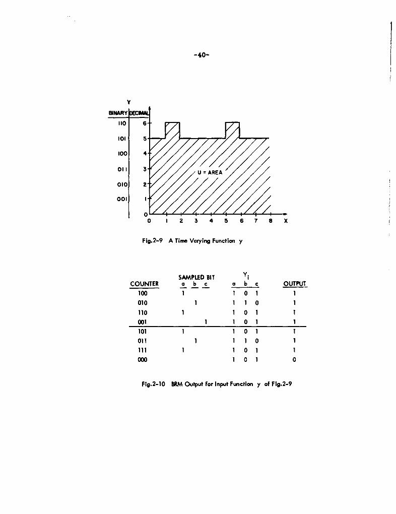
2. Example of Round Off Errors for Time Varying Function
Let us examine our same 3 bit BRM and DDA multiplying a pulse
rate with a time varying function. Consider a function y which starts out at
the value 5. After one input clock it becomes 6, but returns to 5 after the
next input clock. y then remains 5 until the fifth clock when it again
becomes 6 for one clock time andreturns to 5 for the rest of the period.
This function is illustrated in Fig. 2.9. Since y is 5 most of the time one
would expect the output to be 5 pulses with a small remainder error. Actually
the area under the curve of Fig. 2.9 divided by the base represents the exact
value desired for the output U, i.e. 4 2/8 = 5.25 for the time shown. Figure
2.10 depicts the BRM performance. Table 2.5 compares the outputs of the
BRM with the DDA.
From Table 2.5 it can be seen that the DDA gives an accurate output while
holding the exact value of round off error in its R register. The BRM on
the other hand, relying on round-off to average out, puts out pulses based
on the instantaneous value of Y at each clock time. Thus clocks 2 and 6
generate output pulses because at these times bit two of y is a 1. If y had
the value 5 for i = 2 and i = 6 and was 6 for two other clock times, its U ouitput
would be 5 instead of 7.
-40-
YBINARY DE]CIM,
010 626
01 51
000 411
101 31 U 0R1A
010 21
0 000 101-
0 1 2 3 4 5 6 7 8 X
Fig.2-9 A Time Varying Function y
SAMPLED BIT Y iCOUNTER a b c a b c OUTPUT
100 1 1 0 1 1
010 1 1 1 0 1
110 1 1 0 1 I
001 1 1 0 1 1
101 1 1 0 1 1
Oil I 1 0 1
111 11 0 1 1
000 1 0 1 0
Fig.2-10 BRM Output for Input Function y of Fig.2-9

-41 -
Table 2.5
BRM Total DDA Total RemainderY. VY Output U Output U R
i i WJ BRM WLU DDA DDA Actual U
1 5 +1 1 1 0 0 5/8 5/8
2 6 - 1 1 2 1 1 3/8 1 3/8
3 5 0 1 3 1 2 0 2
4 5 0 1 4 0 2 5/8 2 5/8
5 5 +1 1 5 1 3 1/4 3 1/4
6 6 -i 1 6 0 4 0 4.0
7 5 0 1 7 1 4 5/8 4 5/8
8 5 0 0 7 1 5 1/4 5 1/4
It can be seen then that if y is a changing value during integrations, the
DDA is considerably superior to the BRM, while if y is a constant, Tables
2.2 and 2.4 show us there is little to choose between them.
G. SINGLE COUNTER ERM LINE GENERATOR
1. General
The principal disadvantage of the DDA is the amount of hardware it
requires: two registers and one full adder. This does not seem so
different at first glance from the BRM which requires two registers and
sonle gating logic between them for each BRM. Examining the BRM more
-4Z -
closely however we note that one of the two registers is just a counter which
counts input pulses. It seems feasible and well worth our while to share
a single counter between several data registers wherever possible. In
Fig. 2. 7 wer otethere are 4 pulse rates to be counted: the original clock
rate, the x rate, the y rate, and the z rate. This means three registers
can be saved sharing an X counter between ih and iv data registers,
a Y counter between Jh and jv and a Z counter between kh and kv
Furthermore, there is a possibility that we can share a single counter in
the line generator between all 3 data registers. This can certainly be
done for straight line generation since for vector generation the x, y and
z BRM's can all be pulsed simultaneously. In generating second order
curves however we note that the configurations of integrators needed to generate
the proper equations require that each BRM have a unique counter so one
BRM can be processed and its output fed to the second before the second
is pulsed. In the next section we shall examine curve generation using
two BRM's sharing a single counter.
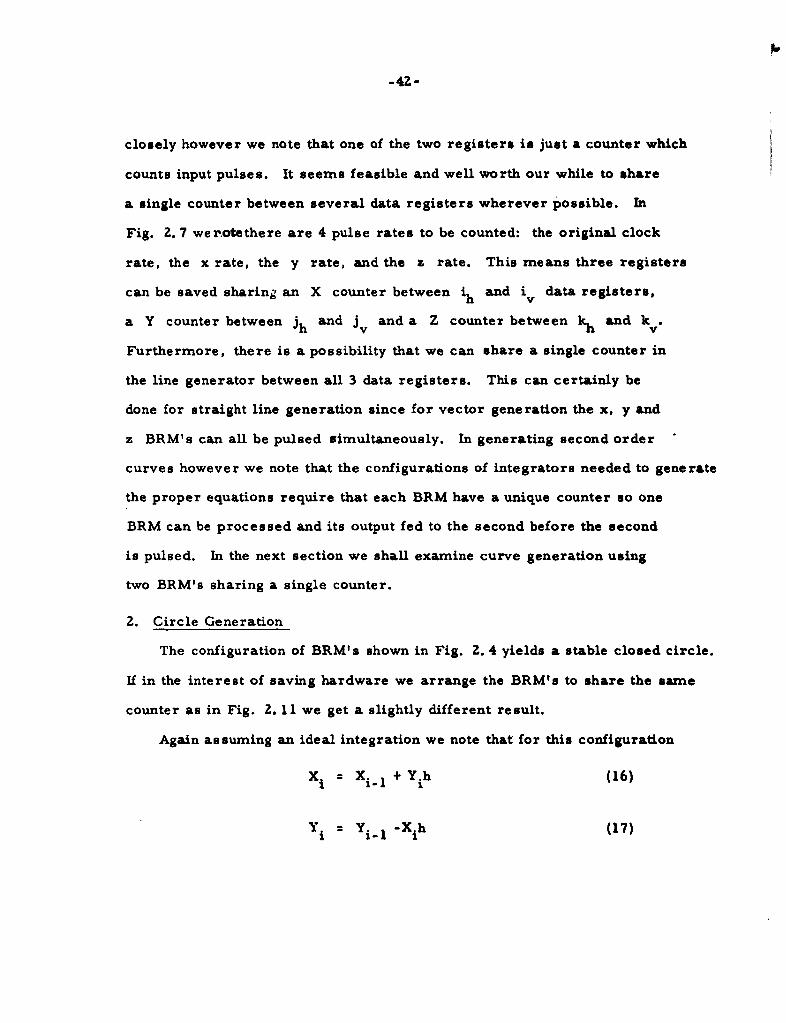
2. Circle Generation
The configuration of BRM's shown in Fig. 2. 4 yields a stable closed circle.
If in the interest of saving hardware we arrange the BRM's to share the same
counter as in Fig. 2. 11 we get a slightly different result.
Again assuming an ideal integration we note that for this configuration
Xi = i.1 + Yih (16)
Y. Y. -Xih (17)
-43-
From Eq. 16 - XXi - i1
Yi I h "
which substituted into Eq. 17 yields
Xi Xi-I Xi-1 -X i-Zxi=~i -~~ - X.h
h h
or X i- 2Xi 11 + (1 + h 2) X i 2 = 0
Substituting Xi = 1i and solving for 1.
S2* 4 2-4(+h2) = lI*jh2
X. C (I +jh)i + C2 (l - jh)i
X= iY (C1 cos 0i + C 2 sin *i) (18)
where j =
and where y= 1 +h 2
and + - tan - 1 .
Note this produces an unstable circle since y. the radius of the circle, is a
monotonically increasing function of i. A scope picture of a circle is
generated in a single sweep, however so repeated cycles are not necessary
and the growth is limited. This still means that the computed circle will
not close exactly, however. We now analyze the actual discrepancy caused
by using a single counter.

-44-
To circumscribe en arc of 211 requires n increments
n0= 2n
211
tan" h
For small h tan- h s h
. Zn (19)
n .
Expanding y in a Taylor series
y = n+h2)n/2=I+.E h 2 + (n/2 &nZ-l) h4 +
y= I + nh + 1 (n-h) h2n 2 +'
yn 1 + nh (20)
Thus the radius at completion of the circle is larger by an added factor
rhx Radius. This might be considered the "method error", since it is a
computation error based on the method of computation used, and is
independent of errors due to the nature of the BRM.
3. Hyperbola Generation
A near hyperbolic function can also be generated by altering Fig. 2.11
to make both feedback paths positive.
The basic equations for ideal integrators become
Xi = X + Yi 1 h (21)
Yi + Yi-I+ Xi- h (22)
-45-
Ji YiY-I +9Y I
-- VU
vt J COUNTER
[ Xi Xi-' +VXi
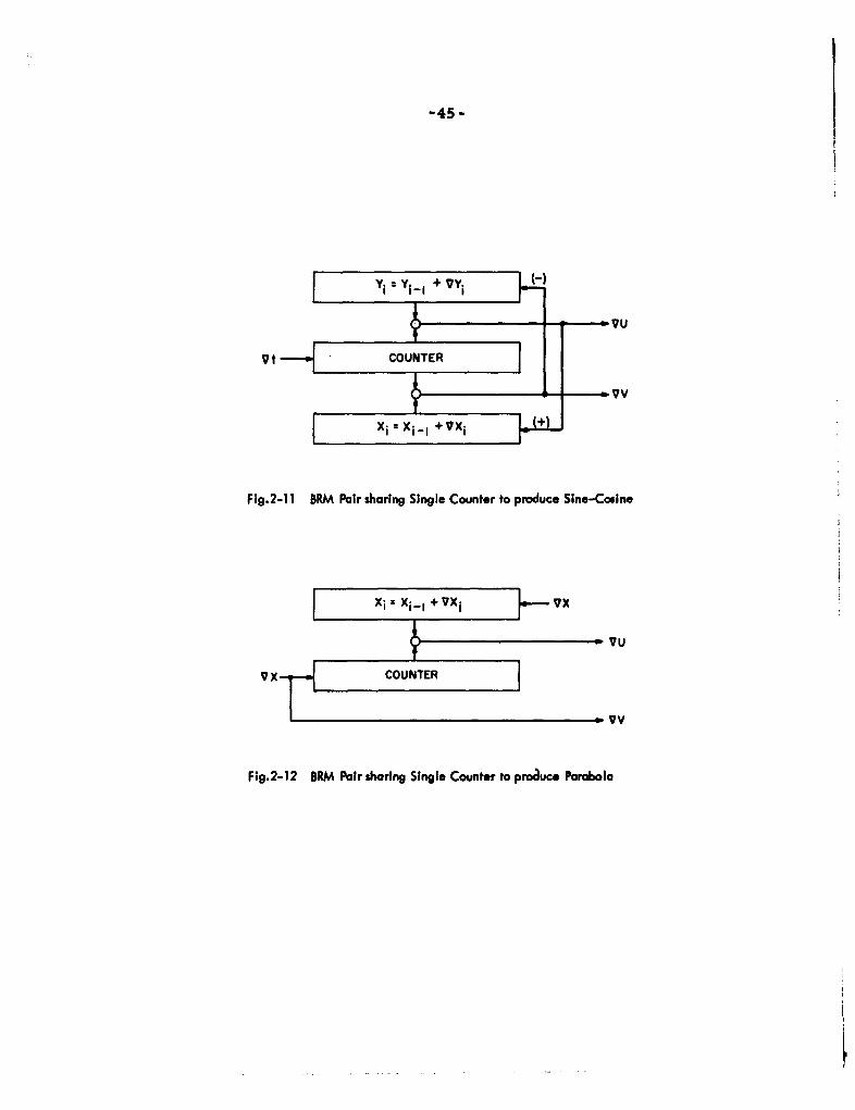
Fig.2-11 BRM Pair sharing Single Counter to produce Sine-Cosine
S Xi " Xi-I + vXi Jm•vx
VU
Fig.2-12 BRM Pair sharing Single Counter to proauce Parabola
-46-
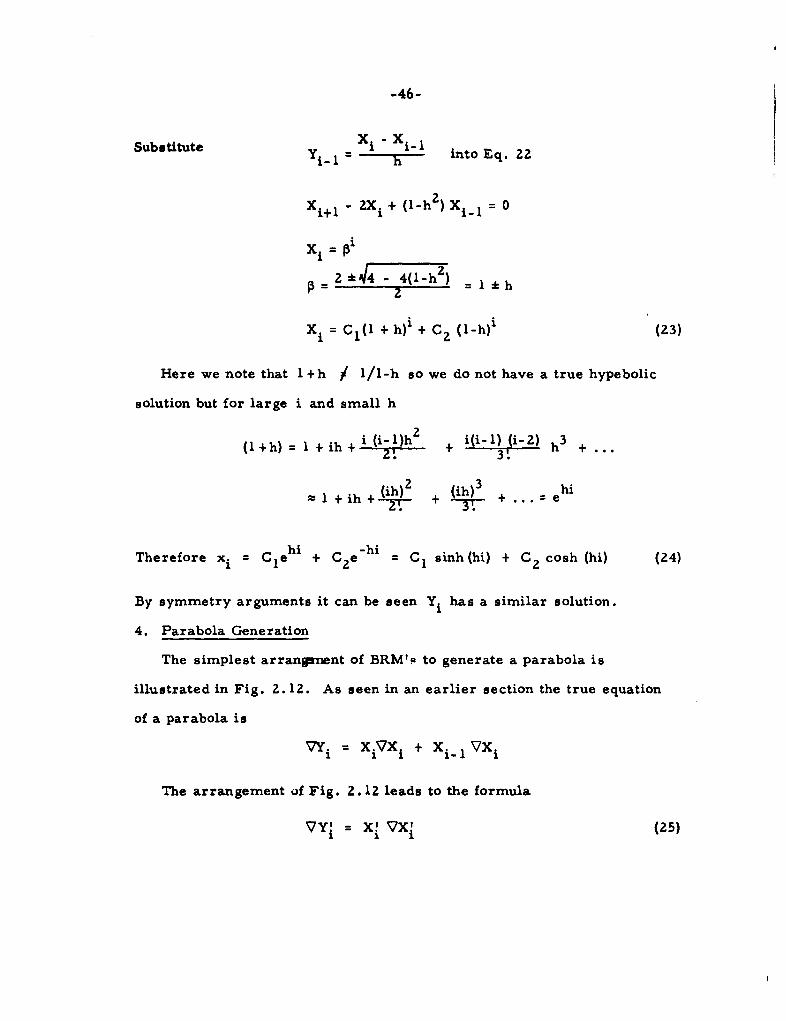
Substitute Xi " Xi-1Yi-I ---- -.. hinto Eq. 22
Xi+l - 2Xi + (l-h 2 ) X1 -I = 0
Xi = Pi
2 44- 4(1-h 2) _1*h
X= Cl(l + h)i + C2 (1-h)i (23)
Here we note that I +h / 1/1-h so we do not have a true hypebolic
solution but for large i and small h
(I+h :I i +i (i- 1)h 2 i(i-1) (i-2) h3+ 2." + 3-... h +.""
l+ih +(ih)2 + (ih)3 + ehi•'-I2 +i+• + +..=
Therefore xi = Ciehi + C 2e-hi = CI sinh (hi) + C2 cosh (hi) (24)
By symmetry arguments it can be seen Yi has a similar solution.
4. Parabola Generation
The simplest arrangrnent of BRM'P to generate a parabola is
illustrated in Fig. 2.12. As seen in an earlier section the true equation
of a parabola is
VY. = X.Vx + x VX1 1. 1 i-l l
The arrangement of Fig. 2.12 leads to the formula
VYi = Xi vx 1 (25)
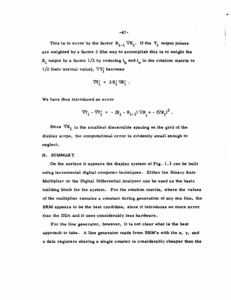
-47-
This is in error by the factor Xi.I VXi. If the Yi output pulses
are weighted by a factor 2 (the way to accomplish this is to weight the
Xi output by a factor 1/2 by reducing ih and iv in the rotation matrix to
1/2 their normal value), VY! becomes1
Vy= 2xl VX
We have thus introduced an error
VYi -VY! - Xi- Xi 1)VX = -(VX
Since VXi is the smallest discernible spacing on the grid of the
display scope, the computational error is evidently small enough to
neglect.
H. SUMMARY
On the surface it appears the display system of Fig. 1. 1 can be built
using incremental digital computer techniques. Either the Binary Rate
Multiplier or the Digital Differential Analyzer can be used as the basic
building block for the system. For the rotation matrix, where the values
of the multiplier remains a constant during generation of any one line, the
BRM appears to be the best candidate, since it introduces no more error
than the DDA and it uses considerably less hardware.
For the line generator, however, it is not clear what is the best
approach to take. A line generator made from BRM's with the x, y, and
z data registers sharing a single counter is considerably cheaper than the
-48-
DDA line generator, BRM's are more susceptible to round-off errors for
time varying multipliers. Furthermore, when a single counter is shared,
a small but ever present computational method error is introduced. The
DDA on the other hand, although more expensive, is much less victimized
by round-off error, since it holds the value of round-off in its R. register
at all times. In addition avoidance of the computational error is more
easily accomplished, since each DDA is entirely independent of the others
except for the basic clock.
To settle these and other questions a computer simulation of the
entire system was programmed for the PDP- 1 Computer. Chapter III
discusses the results of this study.
CHAPTER m
SIMULATION PROGRAM
A. GENERAL
Because of the various choices available for ways of instrumenting
the display system of Fig. 1. 1, it seemed wise to study in more detail the
quality of the pictures produced by each. This way many questions could
be resolved without building hardware. Among these questions are:
a) How bad is the round-off error in BRM generatedcurves?
b) How long should the BRM or DDA registers be toproduce acceptable curves?
c) How objectionable are figures which don't closedue to accumulated errors?
d) How accurate must the rotation matrix multiplybe, i.e. how many bits must these units contain?
e) Are the figures satisfactory after being rotated?
To investigate these questions a program was written for the PDP-I
Computer to simulate the Display System in a number of forms. As
different areas of interest developed, the program changed shape and before
all aspects were investigated several versions of the program had
evolved. The most general of these is described in Appendix A.
B. STRAIGHT LINES
1. Generation
The first task was to examine the quality of the straight lines
generated by the BRM and the DDA. It seemed reasonable to assume,
based on the evidence seen in Tables 2.2 and 2.4, that both devices
-49-

-50-
would give entirely satisfactory results. The smallest error possible is
less than the least significant digit of the generator, which can be made
to represent any size step desired in the scope coordinates. Since
it is desirable to keep the plotting speed as fast as possible, the
least significant digit of the BRM and DDA in the line generator and in
the rotation matrix was made equal to the least significant digit in
the scope register. On the PDP scope this represents a step of about
1/100th of an inch, which, because of the glow of the phosphor, is virtually
indistinguishable. To expand the pictures so that points could be
distinguished, a magnification control was incorporated in the
simulation program which spaced the points twice as far apart or four
times as far apart. Since the PDP-I scope does not have a camera
attachment, photographs were taken on a Tektronix 536 scope unit
which was connected in parallel with the display scope. The amplifier
stages of this scope allowed for further expansion capabilities.
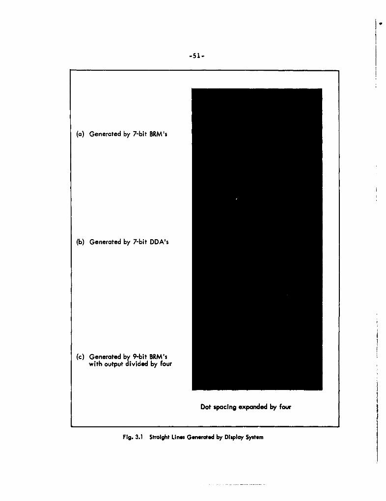
Figure 3. 1 illustrates lines generated by a BRM (a) and a DDA (b)
vector generator. The figure is made up of the following lines (starting
in the lower right hand corner and moving counterclockwise):
Line 1: x = -658, y = 56., z = 0.
Line 2: x = -508, y 158, z = 0.
Line 3: x = 178, y = -60, z = 638.
Line 4: x 1168, y =13, z =-638.
The difference between the BRM and a DDA is perhaps best illustrated
in lines 4 and 1. The occurrence of V y steps on line 4 is particularly
illuminating. The DDA distributes them evenly, while the BRM places
them according to the binary digit sampling logic described in Chapter U.
-51 -
(a) Generated by 7-bit BRM's
(b) Generated by 7-bit DDA's
(c) Generated by 9-bit BRM'swith output divided by four
Dot spacing expanded by four
Fig. 3.1 Straight Lines Generated by Display System

-52-
Line I shows the effects of this difference in distribution when applied to
both x andy. The DDA vector appears thick but smooth. The BRM gives
a more ragged appearance. It should be kept in mind that these pictures
are expanded by a factor of four so that dot spacini, can be easily
distinguished. On the normal scale these two pictures appear virtually
identical.
2. Rotation
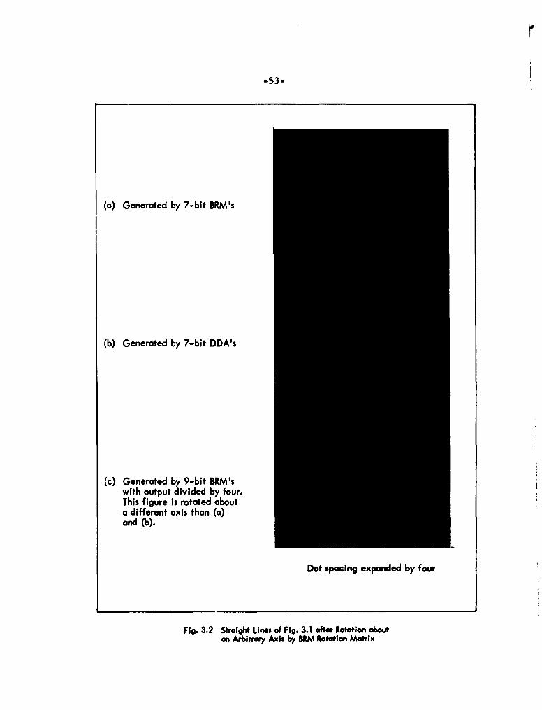
Figure 3.2(a) and (b) shows the same lines of Fig. 3. 1 but after
rotation through some arbitrary angle. The rotation matrix was made
of 8 bit BRM's in each case. This is enough bits to insure there is
no distortion for these lines due to inaccuracy of the multiplication. In
Fig. 3. 2 the extreme raggedness of the lines in both (a) and (b) is some-
what depressing and deserves an explanation. This is due to the fact that
there are three sources for h pulses (ih, jh' kh) each clock time,
each of which may be plus or minus one unit, or zero. Thus the least
significant digit of the h register is liable to some extraneous oscillations.
To see this more clearly consider a simple example.
Consider as before, the crude but illustrative three bit Binary Rate
Multiplier. Assume the entire system of Fig. 2. 7 is made of these and
that we are generating the vector x = 6, y = 3, z = 0. Figure 3. 3 shows
the x and y output pulses that are emitted by the vector generator, and
how they plot on the scope with no rotation.
Now consider this same plot when the line is rotated on the scope
face through an angle of 500 about the depth axis. Although three bit
BRM's will not hold precise values of the rotation terms, their values
-53-
(a) Generated by 7-bit BRM's
(b) Generated by 7-bit DDA's
(c) Generated by 9-bit BRM'swith output divided by four.This figure is rotated abouta different axis than (a)and (b).
Dot spacing expanded by four
Fig. 3.2 Straight Lines of Fig. 3.1 after Rotation aboutan Arbitrary Axis by WM Rotation Matrix
-54-
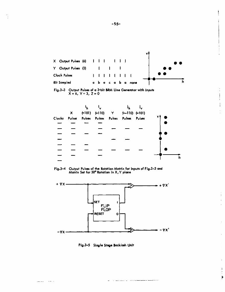
are close enough for our present purposes; ih = 5 (cos 500 = .64 2 5/8),
iv = 6 (sin 500 = .76 z 6/8), 3h = -6, jv = 5.
Table 3. 1 shows the sequence of output pulses that generate the
rotated line, which is shown in Fig. 3.4. Since the first output pulse
from the line generator is an x pulse (see Fig. 3.3), the x counter
(which is the counter register for the ih and i BRM's) increments first.
The 0 to 1 transition of the least significant bit of this counter causes
a + 1 output from both the ih and i BRM since the 4's bit of each is ONE,h v
thereby causing h and v to be incremented. The second clock into the line
generator produces both an x and a y pulse. For the x counter the 0 to 1
transition is in the second digit, and therefore it samples the 2's digit of
ih and iv. Since ih holds the value 1012, no output occurs from that BRM, but
iv, containing 1102, has a ONE in the second place so it will output a +1.
At this clock time a y pulse has also been generated. This causes a -I
pulse from the 3h BRM and a +1 from the jv BRM. The net effect at this
clock time is to step h back to 0 (sum of ih and jh out~uts) and to
increment v by 2 (sum of jv and iv outputs) to the value 3. Continuing
on in this manner generates the ragged line shown in Fig. 3.4.
The crudeness of this line is rather appalling, but it should be
remembered that the spacing shown, when viewed on a normal screen is
barely perceptible. However when three dimensional lines rotated about
three axes are considered, the coarseness gets understandably worse,
as can be seen in Fig. 3.2.
3. Improvements
There are two remedies for this roughness that seemed worth
investigating. One is to compute the increments for h and v to a finer
-55-
X Output Pulses (6) I I I I I 1
Y Output Pulses (3) I 0 0
Clock Pulses I I I I I I I
Bit Sampled a b a c a b a none h
Fig.3-3 Output Pulses of a 3-bit BRM Line Generator with InputsX=6, Y=3, Z= 0
ih iv ih ivX (=101) (=110) Y (=-110) (=101)
Clocks Pulses Pulses Pulses Pulses Pulses Pulses
- 40
h
Fig.3-4 Output Pulses of the Rotation Matrix for Inputs of Fig.3-3 andMatrix Set for 50° Rotation in X,Y plane
+ vX +vX'
SET FLIP
FLOPRESET 0
-vX _ _ _ -v X,
Fig.3-5 Single Stage Backlash Unit

-56-
Table 3.1
X Yi jCounter Counter 'h i v v(i) () +101 -110 h +110 +101 v
001 +I +I +I +I
010 001 0 -1 0 +1 +1 +3
011 +1 +1 +1 +4
010 -1 0 0 +4
100 +1 +1 0 +4
101 011 +1 -I +1 +1 +1 +6
110 0 +1 +1 +7
scale. The second is to incorporate a "backlash" unit to eliminate the
extraneous oscillations.
Computing to a finer scale is accomplished by adding extra bits
to the h and v accumulating registers at the least significant end. The
outputs of the rotation matrix are then introduced into the least significant
of these bits, but the added bits are not displayed. Plotting would not
occur until a carry pulse from these extra bits incremented the original
h or v register. This would cure the raggedness of the plotted line
since the fluctuations of the least significant digits would not be shown.
The principal drawback to this scheme is that for every bit added to h
and v, the display speed is cut in half since it then requires twice as many
outputs pulses to draw the same length line.
-57-
A way around this is to speed up the basic clock rate by an appropriate
amount. Since the display rate, even f-)r our new system, is none too fast,
as we noted in Chapter I, we will already be running the clock at as high a
speed as we can. In Chapter V where some hardware considerations are examined,
it is shown that the highest speed, most critical point in the entire system is right
here where three 1 megacycle pulse trains are summed into a long (10 to 15 binary
bits) counter. Thus increasing the basic clock rate to accomplish smoothing is
not feasible.
The other scheme, using the Backlash Unit, has the attractive feature that
7the display is not slowed by it. The Backlash Unit is suggested by Lundh for a
slightly different application, but it appears appropriate here since in principal it
is a sort of high frequency digital filter. It consists of a single flip-flop plus some
associated gating as illustrated in Fig. 3.5. The flip-flop which is set to the
ONE state by a positive Vx pulse and reset to ZERO by a negative Vx pulse.
Positive pulses trying to pass through this unit are gated by an AND gate whose
other input is the ONE state of the flip-flop. Thus a positive x pulse will be
output only if two successive positive Vx's are input. Similarly a negative Vx
output will occur only after two negative pulses input in a row. The net effect is
to filter out the high frequency fluctuations of the input. A two stage unit can
be built on the same principal for more heavy filtering but we shall not consider
it here. Applying such a unit to the input to the h and v register seemingly
should reduce the coarseness of the rotated straight lines.
Figure 3.6 shows the results of these various techniques. The configuration
of lines is identical to that depicted in Fig. 3.1 and 3.2, but rotated to a new
orientation. The top line is Line 1. Line 2 is the next line in the counter-
clockwise direction and so on around. Figure 3.6 (a) shows the BRM produced
picture unadulterated. The neat appearance of (c) is as expected since the
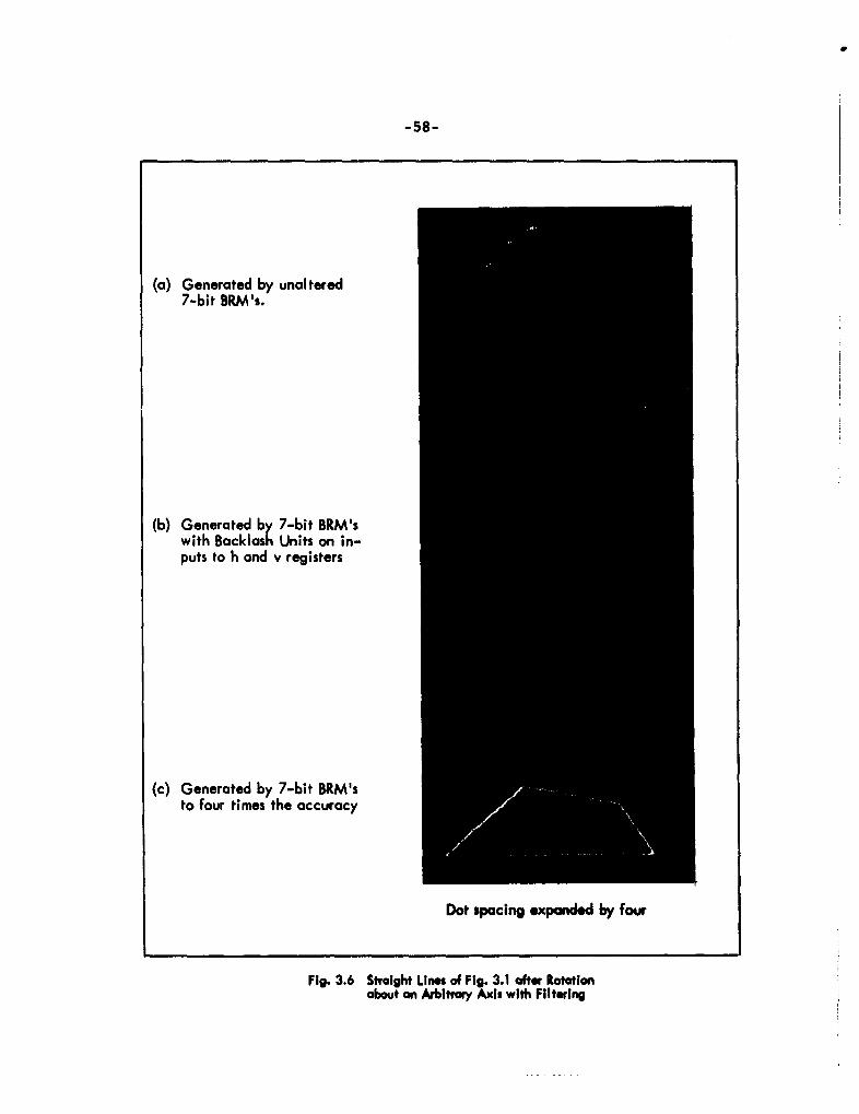
-58-
(a) Generated by unaltered7-bit BRM's.
(b) Generated by 7-bit BRM'swith Backlash Units on in-puts to h and v registers
(c) Generated by 7-bit BRM'sto four times the accuracy
Dot spacing expanded by four
Fig. 3.6 Straight Lines of Fig. 3.1 after Rotationabout an Arbitrary Axis with Filtering

-59-
computations are four times as accurate, but the lines take four times as
long to be drawn. The most intriguing results however are seen in (b),
where the Backlash Unit removes many of the seemingly extraneous points
plotted, but does not really remove any of the coarseness of the lines.
It appeaz that the difficulty is not so much the high frequency oscillations
of the least significant bit being plotted as the non-uniformity in the output
pulse rate of a BRM, principally from the rotation matrix. It is apparent
that some sort of smoothing technique is highly desireable.
The conclusion to be drawn from this section is that a compromise must
be made between plotting speed and coarseness of the rotated lines. More
accurate lines may be drawn at a slower speed. In Chapter IV smoothing
techniques for the Binary Rate Multiplier are considered. A feasible
smoothing device is discussed but it entails a considerable amount of
added hardware, so that it again becomes an engineering compromise
based on an evaluation of the seriousness of the problem. It is the
authors opinion that on the normal scale, the raggedness of the lines is
barely noticeable and does not warrant slowing the display or the expense
of adding smoothing logic on the output of each BRM of the rotation matrix.
C. SECOND ORDER CURVES
1. BRM Curve Generation
To study the errors in the gerieration of second order curves, the
circle was chosen as the best representative. This is because it is
easiest to evaluate from a purely visual comparison. This is particularly
true in examining the closure of the circle.
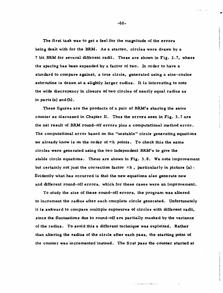
-60-
The first task was to get a feel for the magnitude of the errors
being dealt with for the BRM. As a starter, circles were drawn by a
7 bit BRM for several different radii. These are shown in Fig. 3.7, where
the spacing has been expanded by a factor of two. In order to have a
standard to compare against, a true circle, generated using a sine-cosine
subroutine is drawn at a slightly larger radius. It is interesting to note
the wide discrepency in closure of two circles of nearly equal radius as
in parts (a) and (b).
These figures are the products of a pair of BRM's sharing the same
counter as discussed in Chapter II. Thus the errors seen in Fig. 3.7 are
the net result of BRM round-off errors plus a computational method error.
The computational error based on the "unstable" circle generating equations
we already know is on the order of nh points. To check this the same
circles were generated using the two independent BRM's to give the
stable circle equations. These are shown in Fig. 3.8. We note improvement
but certainly not just the correction factor rh , particularly in picture (a) •
Evidently what has occurred is that the new equations also generate new
and different round-off errors, which for these cases were an improvement.
To study the size of these round-off errors, the program was altered
to increment the radius after each complete circle generated. Unfortunately
it is awkward to compare multiple exposures of circles with different radii,
since the fluctuations due to round-off are partially masked by the variance
of the radius. To avoid this a different technique was exploited. Rather
than altering the radius of the circle after each pass, the starting point of
the counter was incremented instead. The first pass the counter started at
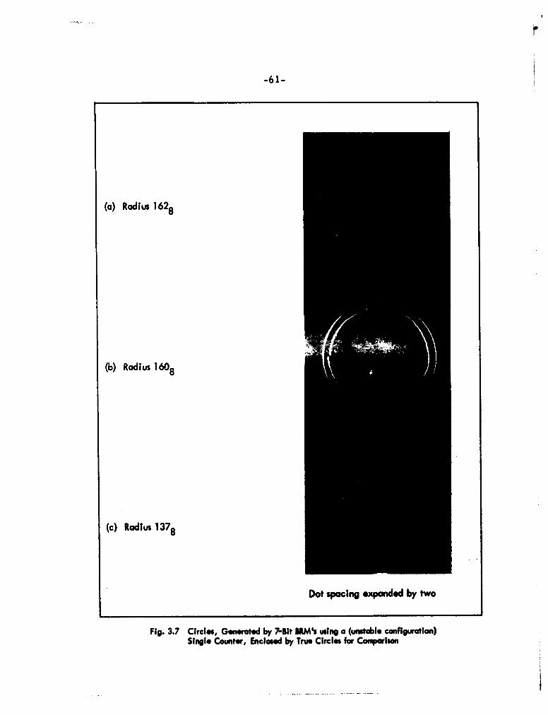
-61-
(a) Radius 1628
(b) Radius 1608
(c) Radius 1378
Dot spacing expandd by two
Fig. 3.7 Circles, Generated by 7-Bit BRM's using a (unstble configuration)Single Counter, Enclosed by True Circles for Coporiown

-62-
(a) Radius 1628
(b) Radius 1608
(c) Radius 1378
Dot spacing expanded by two
Fig. 3.8 Circles, Generated by 7-Sit BEM's using SeparateCounters (stable configuration), Enclosed by True Circles
-63-
zero and counted to 2/h. The next pass it started at one and counted
to 2/h + 1, and so on. This isolated the variance in the circles to
round-off errors alone, since the radius is held constant. To eliminate
computation method error, the stable circle configuration was used.
Figure 3.9 6) and(b) show circles of radius 1358 and 1438 generated
on a BRM with varying counter initial conditions. As can be seen from
these photographs, the BRM round-off error at closure can be as much as
1/10 of the radius of the circle, even though h is only 1/128.
If an 8 bit, rather than a 7 bit BRM were used to generate the same
sized circle, precisely the same picture would be produced. This is
because the most significant bit of the BRM (i.e. the most significant bit
of the data register, which is the one sampled f/2 times by 0 to 1 transitions
of the least significant bit of the BRM counter) is always zero. Thus every
other input pulse is used on 0 to 1 transitions of the least significant bit
of the 8 bit BRM counter. The rest of the input pulses act on the remaining
7 active bits of the BAM. All that is accomplished is to require twice
as many input pulses to complete the circle.
2. Improvements for the BRM Curves
There is a plan however which can be applied to reduce round-off errors.
Consider an 8 bit BRM containing a radius twice as large as that in Fig. 3.9 (b)
(i.e. 3068). Since the round-off error is essentially unrelated to
the size of the circle, the error in the 8 bit BRM should be of the same
general magnitude as that of the 7 bit BRM. If the output pulse trains are
then divided by two I.e., only every other one is used to increment h or v
the radius is brought back down to the original size, and the round off
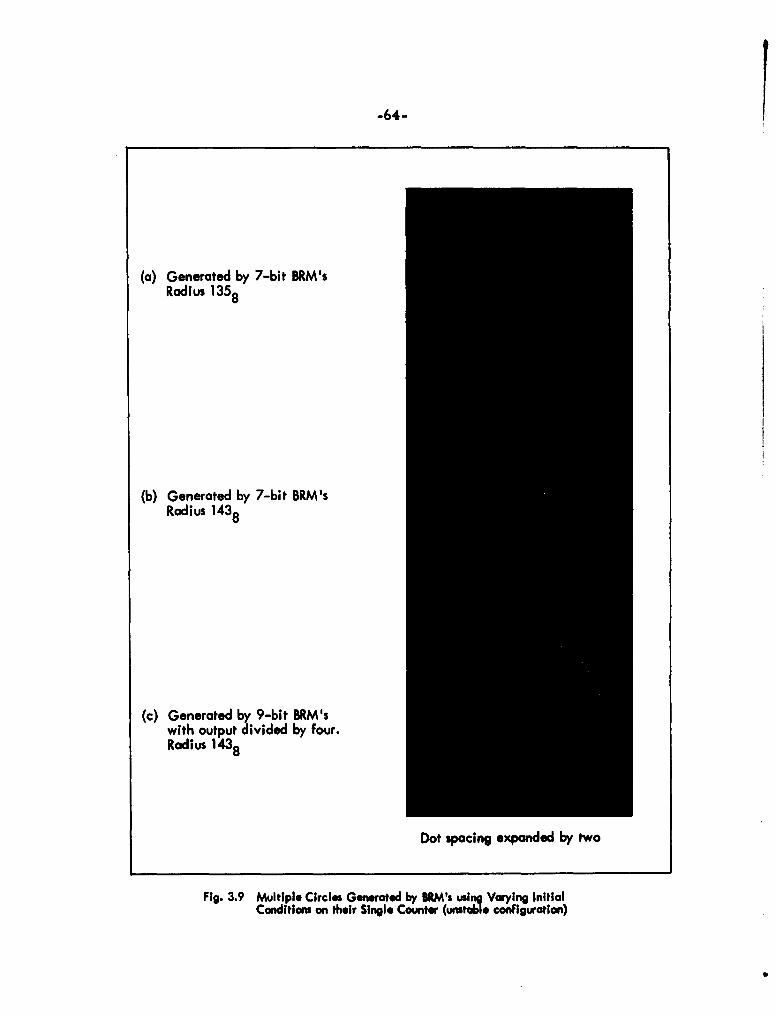
-64-
(a) Generated by 7-bit BRM'sRadius 1358
(b) Generated by 7-bit BRM'sRadius 1438
(c) Generated by 9-bit BRM'swith output divided by four.Radius 1438
Dot spacing expanded by two
Fig. 3.9 Multiple Circles Generated by BRM's using Varying InitialConditions on their Single Counter (unstable configuration)

-65-
error is halved. This procedure can be applied as often as desired,
but each factor of two improvement added slows the display by a like amount.
Figures 3.9 (c) and 3.10 illustrate the effectiveness of this technique.
A circle of radius 1528 generated by a 7 bit BRM is shown in Fig. 3. 10 (a).
Picture (b) is produced by an 8 bit BRM using a radius 3248 (twice 1528),
but divided by two in the rotation matrix where ih = iv = 1/2, and all other
components are zero. Figure 3.10 (c) is the output of a 9 bit BRM with
a radius of 6508, and divided by four in the rotation matrix. Figure 3.9 (c)
is a picture of the 9 bit BRM circle with an effective radius of 1438, the
same as shown in Fig. 3. 10 (b). The improvement in picture quality is
not without cost however. The extra two bits mean more hardware for the
BRM, and the longer BRM means either slower plotting or requires higher
speed circuitry. It seems appropriate next to compare these results with
thosL of the DDA.
3. DDA Curve Generation
From the discussion of the DDA in the last chapter it seems likely that
the circle generated by a DDA is more true than a circle produced by a
BRM of the same size. To illustrate this and compare the circle made by
the longer BRM, the picture shown as Fig. 3.11 was taken. Part (b) shows a
7 bit DDA circle of radius 1528 lying just inside a true circle. Parts (a) and
(c) are the same circle as created by a 7 bit BRM and by a 9 bit BRM that
has been reduced by a factor of four by the rotation matrix. These
circles were all generated from the "stable" configuration.
Figure 3.12 is an expansion of Fig. 3. 11 but with a different radius (1608) .
This reveals the same coarseness of lines on the BRM produced curve as we
saw on the straight lines. The technique of creating a larger circle and then
reducing it back down to size seems to smooth out the curve so that it

-66-
(a) Generated by 7-bit BRM'sRadius 1528
(b) Generated by 8-bit BRM'swith output divided by two.Radius 1528
(c) Generated by 9-bit BRM'swith output divided by four.Radius 1528
Dot spacing expanded by two
Fig. 3.10 Multiple Circles Generated by ERM's using Varying InitialConditions on their Single Counter (unstable configuration)
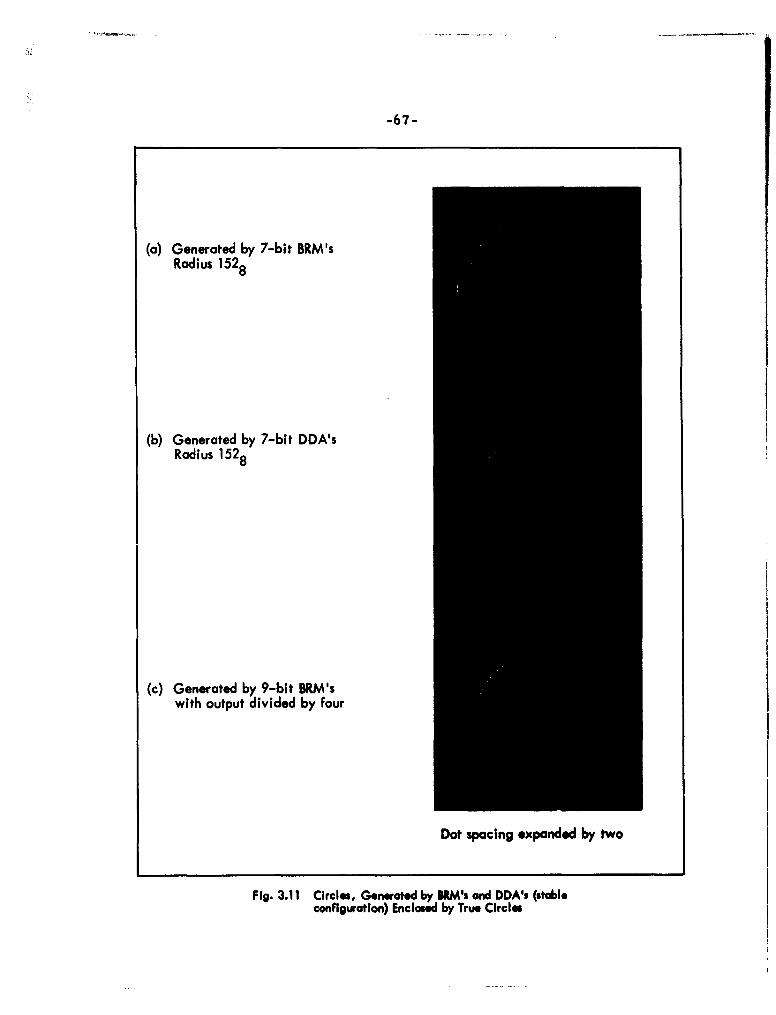
-67-
(a) Generated by 7-bit BRM'sRadius 1528
(b) Generated by 7-bit DDA'sRadius 1528
(c) Generated by 9-bit BRM'swith output divided by four
Dot spacing expanded by two
Fig. 3.11 Circles, Generated by IRM's and DDA's (stableconfiguration) Enclosed by True Circles
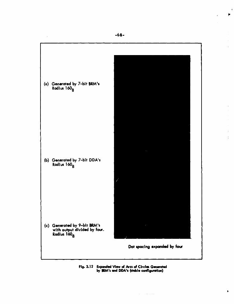
-68-
(a) Generated by 7-bit BRM'sRadius 1608
(b) Generated by 7-bit DDA'sRadius 1608
(c) Generated by 9-bit BRM'swith output divided by four.Radius 1608
Dot spacing expanded by four
Flo. 3.12 Expended View of Arcs of Circles Generatedby WMs and DDA's (stable conflgiration)
-69-
compares favorably with the DDA. Going back to Figs. 3.1 and 3.2, the
straight line figure of these pictures was also generated using this
technique. It can be seen to be quite similar to the DDA lines, evenly
spaced and thick.
4. Computation Method Error
The question of the computational method error is still to be
considered. As discussed in Chapter II, this error is introduced when the
x and y integrators (BRM or DDA) are processed at the same time. The
error is avoided by first dealing with x and using its result to alter y,
before y is processed. For the system using separate integrators for
x, y and z this error is easy to avoid, since each can be processed in
whatever order desired. For the BRM line generator using a single
counter, however, this error can not be so easily eliminated, since the
0 to 1 transition of the counter will instantaneously sample both data
registers. It is possible to delay the sampling of one of the registers
by suitable tricks in the hardware, but this adds to the expense of the unit.
Fortunately the technique applied to reduce round-off error also
lessens the computational method error. This can be seen by recalling
Eq. 20 of Chapter II which shows the amount of the method error in the
case of a circle to be:
e = 1rRh
where R is the radius of the circle expressed as a binary fraction (always
less than ONE) and h is the fractional value of the least significant bit.
Generating a circle with a larger BRM and then reducing the resultant
outputs is essentially computing to more bits of accuracy and then disregarding
the least significant bits.

S1*-70-
Thus suppose a circle of radius 2k is desired and a BRM pair, each
of length k + 2 bits are used to compute a circle of full radius, the output
of the line generator being divided by four to re-establish the radius at
k2 . The computation method error will be r . Since a single
1 2 +2increment on the scope grid is weighted as-• , the error in scope units
2becomes
2
This is born out in Fig. 3. 10 (c), where the BRM closure is excellent.
D. ROTATION MATRIX
A large part of the flexibility of the proposed system stems from the
computer's ability to alter the contents of the rotation matrix BRM's. The
question arises just how accurate the computations they perform must be, i.e.,
how many bits in length to make the BRM's. It appears that the fewer the bits,
the coarser the quantization of the rotation, but it is not clear whether lines
will be distorted by short BRM's or whether errors will be introduced so
that figures will no longer close.
To check the effect of BRM's of various lengths in the rotation
matrix, the program was altered to simulate using BRM's of 2 bits,
3 bits, 6 bits and 12 bits. Figure 3.13 is a picture of an identical
tetrahedron rotated the same amount, but using these different BRM's.
The figures are seen to differ in the angle, the length, and the coarseness
of the lines. But in all cases the figures close. The top corner of picture
(c) is off the field of view of the scope camera. A rotation matrix using

L
-71-
(a) 2-bit BRM's in RotationMatrix
(b) 3-bit BRM's in RotationMatrix
(c) 6-bit BRM's in RotationMatrix
Dot spacing expanded by four
Fig. 3.13 Tetrahedron, Generated by SRM's, after Rotation about an ArbitraryAxis by Rotation Matrix consisting of MBM's of Various Lengths

-72-
12 bit BRM's will introduce no errors since they compute to an accuracy
of 1/212 = 1/4096 which for the lines shown is considerably smaller than
a single increment on the display scope grid. The 6 bit machines give
essentially an identical picture as the 12 bit BRM's. This is to be expected
since the most their outputs can differ by is 1/26 = 1/64, which is barely
perceptible.
A bit of reflection on the BRM process will substantiate these results.
The 2 bit unit is identical to a 6 bit BRM with the last 4 bits
equal to zero. Thus 1/4 of the input pulses always produce zero output
from the 2 bit machine, while they may or may not be zero in the larger
unit. For the 3 bit ERM 1/8 the input pulses do not get sampled. Therefore
the line lengths are shorter by the number of these unsampled pulses, which
would have caused a ONE output in the longer BRM. The lines appear coarser in
the longer BRM's since it is these higher order bits that produce the
irregularities as we noted in our earlier studies. The closure is not
affected since the process is reversible, i.e., the same function of positive
(plus direction) input pulses are unsampled as negative (opposite direction)
input pulses. So long as the figure closes in the fixed space x, y, z; the
number of positive input pulses to each rotation matrix BRM will equal
the number of negative input pulses, hence closure is assured.
The decision as to how many bits in length the BRM's of the
rotation matrix should be, is again somewhat arbitrary, depending on how
precisely the eye can detect differences in lines. It seems that a length
of between 6 bits (1/64 = I.5 ¶. and 8 bits (1/256 = .39%1 is sufficient.

r
-73-
E. GENERAL FIGURE DRAWING CAPABILITIES
So far this chapter has been concerned with the differences between
ways of implementing the display system outlined in Chapter Il.
This section is devoted to illustrating the capabilities of the system,
without regard to which "basic unit" is used, by demonstrating a few
of the figures which were produced by the simulation program.
The figures are all generated by a display list headed by a set of
rotation matrix values and followed by a string of line descriptors, as
discussed in Chapter I1. Rotation is achieved by simulating six bit
Binary Rate Multipliers as the basic unit of the rotation matrix unit.
The line generation is done by simulated DDA's or BRM's as specified
in each picture.
Figure 3.14 (c) shows a parabolic sheet generated by a BRM line
generator. This is constructed from ten basic lines, which are identified
in Fig. 3.15. "a" is a parabolic line in the x, y plane. "b" is a straight
line in the plus z direction. "c" is the same parabolic line as "a" but in
the opposite direction. "d" closes the figure by being identical with "b"
but in the minus z direction. Line "e"l uses parameters similar to line
"Ila" except that it is made one fourth the length and is surpressed from
being plotted. '"f" then crosses over a line "c", where "g" is drawn,
again as a blank line. The initial conditions on "tg", are made to coincide
with the end conditions of line "ae", so that it can be considered an extension
of "ett, displaced in z. Lines "h", "i"l, and "j"t continue in this vein.

-74-
(a) Generated by 7-bit DDA's
(b) Generated by 9-bit BRM's
(c) Generated by 9-bit DDA's
Fig. 3.14 Figures Generated by Display System

-75-
d
f C.
ba
Fig.3-15 Breakdown of Unes used to produce F1g.3-14 (c)
fi
g ~d e
h C
ab
Fig.3-16 Breakdown of Unes, used to produce Fig.3-14 (b)
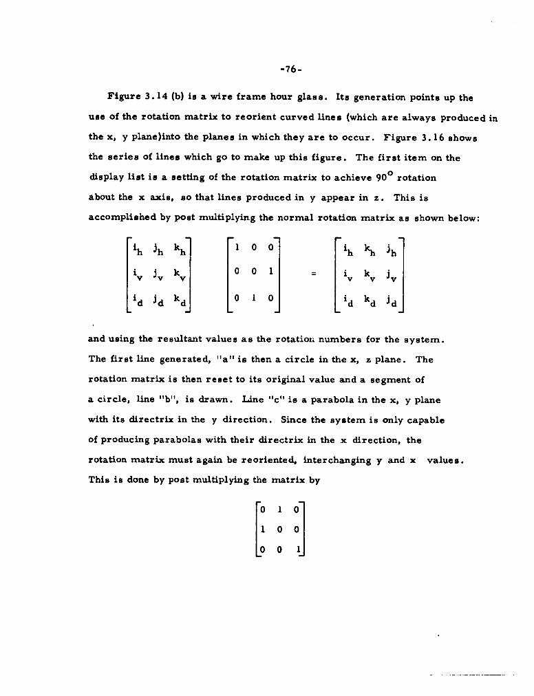
-76-
Figure 3.14 (b) is a wire frame hour glass. Its generation points up the
use of the rotation matrix to reorient curved lines (which are always produced in
the x, y plane)into the planes in which they are to occur. Figure 3.16 shows
the series of lines which go to make up this figure. The first item on the
display list is a setting of the rotation matrix to achieve 900 rotation
about the x axis, so that lines produced in y appear in z. This is
accomplished by post multiplying the normal rotation matrix as shown below:
ih Jh kh 1 0 0 1h kh ih
iv Jv kv 0 0 1 iv kv jv
id id kd 0 1 0 id kd id
and using the resultant values as the rotation numbers for the system.
The first line generated, "a" is then a circle in the x, z plane. The
rotation matrix is then reset to its original value and a segment of
a circle, line "b", is drawn. Line "c" is a parabola in the x, y plane
with its directrix in the y direction. Since the system is only capable
of producing parabolas with their directrix in the x direction, the
rotation matrix must again be reoriented, interchanging y and x values.
This is done by post multiplying the matrix by[0 51o
0o

-77-
The parabola produced by the line generator is the curve
1 2y=•x
If a different parabola is desired (i.e. a different ratio between y and x2 ),
this is also done by changing the rotation numbers. Thus if the curve
2y = x
is intended, the x output of the line generator should be reduced by
while the y output (-2 x 2 ) is not changed. This is done by multiplying the
1first column of the rotation matrix (i terms) by 7z. This can be combined
with the matrix used to reorient x and y which results in a single matrix
10
00
To orient the parabola "c" properly the display list must first set
the rotation matrix to these resultant new values. Then line "c", the
appropriate parabola segment, follows. The next item on the display
list changes the rotation matrix back to the original state. Then line "d",
a segment of a circle similar to "b"' but with different initial conditions,
is given. Following tids, the rotation matrix is changed to the same
values it had for line"a", and "e", another circle in the x, z plane, is
drawn. "f " is then a blank half circle to get the plot around into position
for curves "g', "h" and Ili". This second side is done in a manner
similar to the way that lines "b", "c" and "d" were drawn.
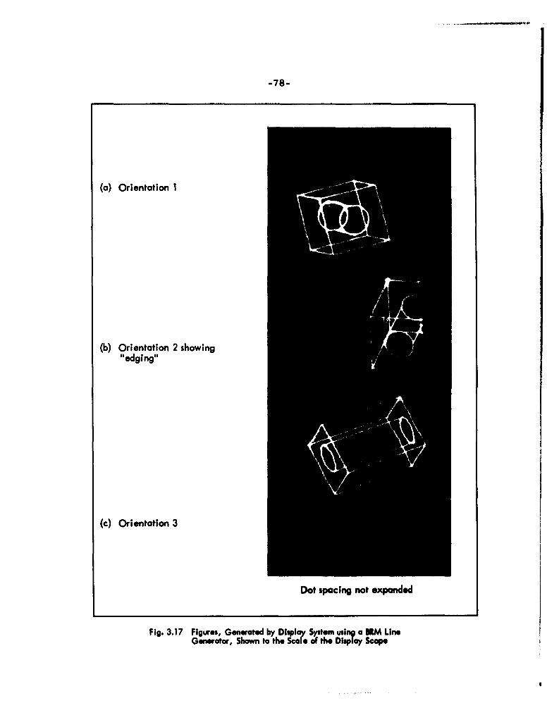
-78-
(a) Orientation I
(b) Orientation 2 showing"edging"
(c) Orientation 3
Dot spacing not expanded
Fig. 3.17 Figures, Geneated by DiW System using a IM LineGenerator, Sh3wn to the Sale of the Display Scone
-79-
Figure 3.14 (b) illustrates one of the weaknesses of this system.
The figures drawn are good wire-frame figures, but do not depict solid
figures well. Solid figures are better shown by drawing their outside edges
and all non-hidden intersections of surfaces. The problem of generating
the outside edge for a second order surface at any rotation is a difficult
one, however, and beyond the abilities of any simple machine. This would
imply that the computer should determine this line and then approximate it
with a line which the system can produce. Identification of hidden lines
is also too difficult a problem for our system. About the best that could
be done is to put into the hardware equipment to generate dotted lines on
command.
Figure 3.14 (a) shows a pair of circles at right angles to each other,
rotated about some arbitrary axis.
Figure 3.17 shows a line depiction of a box with a hole through it at
several orientations. These pictures are shown at the same size as they
appear on the scope face to better illustrate the quality of the pictures displayed.
They have not been subjected to any expansion in spacing between dots. It
can be seen that the roughness of the lines discussed earlier in this chapter
is really quite small and not disturbing to the eye when viewed at normal scale.
Figure 3.17 (b) illustrates the effect of "edging" as performed by the simulated
display system.
CHAPTER IV
BINARY RATE MULTIPLIER ERROR ANALYSIS
A. INTRODUCTION
Because of the significant amount of hardware that can be saved by using
the BRM instead of the DDA, it seems worthwhile to study the BRM in more
detail in hopes of finding ways of improving its performance. There are two
major deficiencies of a BRM as a computing element that the DDA does not
possess. The first is lack of a uniform distribution of the output pulses. The
second is the uncontrolability of the round-off errors when the data register
contains a time varying value. We have seen that by scaling we make these
problems negligible in practice, but improved BRM performance is of general
interest and might have practical benefits as well.
If we consider the generation of a circle by a BRM and a DDA, the two
weaknesses of the BRM are placed in evidence. The non-uniformity of the
output pulse distribution from the x register causes slight errors in the y
register, since this x output represents the change in y. Since this Vy rate is
not smooth, y itself does not change smoothly. The round off errors on the
other hand are bad in the BRM because it has no memory of how much rounding
off is done, whereas the DDA keeps track of this value in its R register Both
of these effects lead to distortions of the circle.
In this chapter we shall address ourselves to these problems and consider
possible solutions. In the latter portion the results of simulation of some of
these solutions are described.
B. SMOOTHING OUTPUT PULSE DISTRIBUTION
1. Output Pulse Distribution
Consider once again the three bit Binary Rate Multiplier containing the value
5. The distribution of output pulses, as seen in Fig. Z. 3, is not as even as might
-81-
-82-
be desired, but since there are only 8 discrete possible clock times on which to
distribute the 5 pulses, there really is no way to improve it. Suppose however
we have a four bit BRM containing the value 5. Then the most significant bit is
ZERO and the output pulse distribution is of the form illustrated in Fig. 4. 1.
The spacing between output pulses is relatively the same as for the 3 bit
BRM, but now there are clock pulses which are between the data pulses. It
would be an improvement (i. e. more close to a perfect integrator output) if
the output were somehow altered so that the pulses were distributed more
evenly as shown in Fig. 4.2.
It can be seen from this example that if the data register contains a ONE in
its most signficant bit there is no way to improve the output pulse distribution
and stay synchronized to the input clocks. If on the other hand at least the most
significant bit holds a ZERO, there exists unused pulse positions which can be
used for smoothing.
2. An Algorithm for Smoothing
Consider the following algorithm for smoothing. "To determine the clock
time on which to output a specific pulse from a modified BRM, look at the position
of the output pulse before and the output pulse after the said pulse on the normal
BRM, and position the said output pulse halfway between these. The first and
last pulses are to be output at the same time as they are in the unaltered BRM."
Thus in Fig. 4. 1 the output pulse on clock 2 is left where it is, but the
pulse generated by clock 6 is spaced halfway between output pulse 2 and output
pulse 8. This relocates the pulse from clock 6 to clock 5. The pulse generated
on clock 8 is positioned halfway between clocks 6 and 10 which means it is not
changed. The pulse produced by clock 10 however is placed midway between 8
and 14, hence occurs at clock 11. The result is just the distribution shown in
Fig. 4. 2.
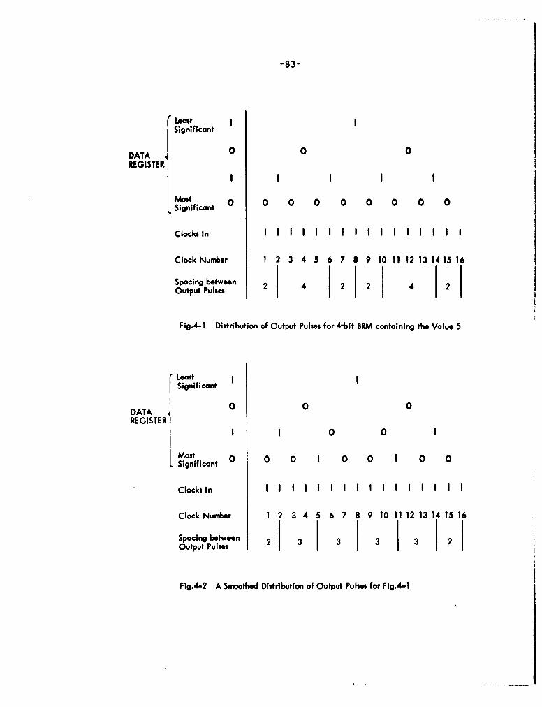
-83-
leastSignificant
DATA 0 0 0REGISTER
II I I I
most 0 0 0 0 0 0 0 0 0Significant
ClocksIn I I I I I I I I I I I I I I I
Clock Number 1 2 3 4 5 6 7 8 9 10 11 12 13 1415 16
Spacing between 2 4 2 2 4 2Output Pu Ises
Fig.4-1 Distribution of Output Pulses for 4-bit BRM containing the Value 5
LeastSignificant
DATA 0 0 0
REGISTERI 1 0 0I
Most 0 0 0 1 0 0 0 0SSignificant
ClocksIn IIIIIIIIIIIIIIII
Clock Number 1 2 3 4 5 6 7 8 9 10 11 12 13 14 15 16
Spacing between 2 3 3 3 3 2Output Pulses
Fig.4-2 A Smoothed Distribution of Output Pulses for Fig.4-1
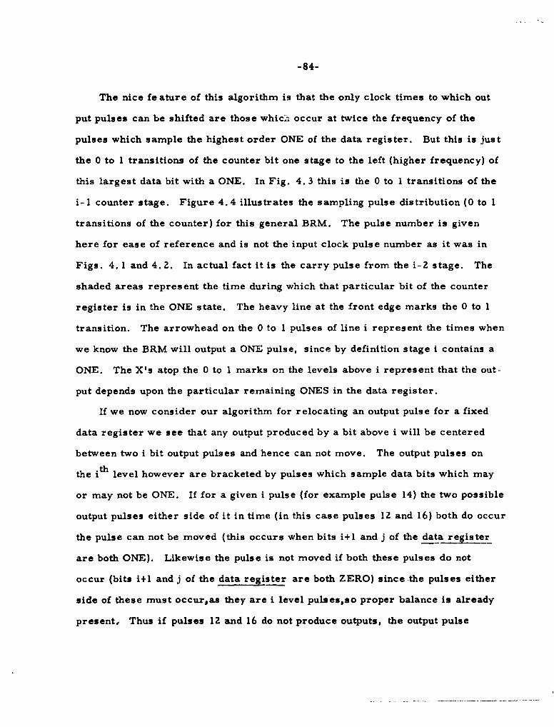
-84-
The nice feature of this algorithm is that the only clock times to which out
put pulses can be shifted are those whic.:i occur at twice the frequency of the
pulses which sample the highest order ONE of the data register. But this is just
the 0 to 1 transitions of the counter bit one stage to the left (higher frequency) of
this largest data bit with a ONE. In Fig. 4. 3 this is the 0 to 1 transitions of the
i- 1 counter stage. Figure 4.4 illustrates the sampling pulse distribution (0 to 1
transitions of the counter) for this general BRM. The pulse number is given
here for ease of reference and is not the input clock pulse number as it was in
Figs. 4. 1 and 4.2. In actual fact it is the carry pulse from the i-2 stage. The
shaded areas represent the time during which that particular bit of the counter
register is in the ONE state. The heavy line at the front edge marks the 0 to 1
transition. The arrowhead on the 0 to 1 pulses of line i represent the times when
we know the BRM will output a ONE pulse, since by definition stage i contains a
ONE. The X's atop the 0 to I marks on the levels above i represent that the out-
put depends upon the particular remaining ONES in the data register.
If we now consider our algorithm for relocating an output pulse for a fixed
data register we see that any output produced by a bit above i will be centered
between two i bit output pulses and hence can not move. The output pulses on
the ith level however are bracketed by pulses which sample data bits which may
or may not be ONE. If for a given i pulse (for example pulse 14) the two possible
output pulses either side of it in time (in this case pulses 12 and 16) both do occur
the pulse can not be moved (this occurs when bits i+l and j of the data register
are both ONE). Likewise the pulse is not moved if both these pulses do not
occur (bits i+l and j of the data register are both ZERO) since the pulses either
side of these must occur,as they are i level pulses,so proper balance is already
present,. Thus if pulses 12 and 16 do not produce outputs, the output pulse

-85-
DATA REGISTER
Od bd Cd ('-')d id (i+l)d (J')d id kd
o 0 0 " - I -" X I 1 X
C
S _ ,
cc bc cc . .*H i) c ýifl i~)c iH c ***
COUNTER
Fig. 4.3 K-Bit BRM Containing some Arbitrary Value
COUNTERBIT X
I I I II I
lII II I1
I I I II
1+2
I I II I a I I A I I I I a I I I I I I I ] .
PULSENO. 1 2 3 4 5 6 7 8 9 101112 1314 15161718192021 2223242526272829303132
Fig. 4.4 Distribution of Sampling Pulses for General BRM
-86-
created by pulse 14 is already centered between pulses 10 and 18 and should not
be moved.
Output pulses do get moved when one of the possible output pulses either
side of the chosen data pulse occurs and the other does not (i. e. either pulse 12
produces an output and pulse 16 does not, or vice versa. This implies either
i+1 is ONE and j is ZERO or j is ONE and i+l is ZERO). In this case the output
pulse is made to occur either one pulse earlier or one pulse later than normal
(in our example it would occur on pulse 13 if i+1 is ZERO and j is ONE, or on
pulse 15 if i+l and j are reversed).
Unfortunately the logic for producing this algorithm is not simple. To
identify that an early output pulse should be generated at an i- 1 level transition
time (e.g. pulse time 13 if i+l of the data register is ZERO and j is ONE in the
example above), logic must be included to identify that i is the most significant
bit of the data register containing a ONE, that this 0 to 1 transition is at the i- 1
level, that i+l of the data register is ZERO and j is ONE, and that of all the
i-1 level sample pulses produced this is one occurring between a sampling of
the i+l data bit and the j data bit. This logic must then be duplicated for all j
between i+2 and k, the least significant bit of the BRM. Furthermore a similar
set of logic must be incorporated for the case where i+l is ONE and j is ZERO,
and another complete pair of logical equations must be mechanized to identify
that a late output pulse should be generated at an i- 1 level transition time.
Boolean equation 26 is the logical equation for the i -I counter bit to identify
that an output pulse which is not generated by normal BRM logic should be pro-
duced.

-87-
Output pulse added if:
(i-I pulse) ad, bdCCd... (i-1)d. id. (i+l)d.Jd[ic(i+l) c...(j-*)cJc
+ (i-I pulse) ad. bd.cd... (T1ld. id. (i+l)d.d [ic. (i+l)c... (-1l)c c]
+ (i-I pulse) d.dd... di-'•d d (i+l-)-• Jd (d[-c" (+l)' 1)c'
+ (i-I pulse ad. bd. Cd...(i-')d.id. (i+')d.Jd[ic. (Fl')c"." (i'- )c'Jc ( 26)
where subscript d identifies data register bits and subscript c counter bits
as in Fig. 4.3.
In addition to this horrendous bulk of logic, there must also be a similar
set to identify when i level output pulses which normally would appear are to
be delete d because they represent pulses which have been moved ahead or
behind to accomodate the smoothing. The following boolean equation applies.
Delete output pulse if:
(i pulse) a ad'b d. C d... (i---1)d' i d. (i+l)d. J'd" -c" ('+'•)c"" (J--'')c" Jc]
+ (i pulse) . ad.bd. Cd...'' l)d. id' (i+l)d. 'd. [icP(i+")c''" (Jl)c Jc]
+ (i pulse) . ad. bd. Cd... ()d. d. (+') d •[-c (i+l)c" (j" 1)c" c]
+ (i pulse) ad.bd.cd... (i--)d.id. (i+l)--d. 3d" [i (i+l)' (J1l)c Jc]
( 27)
This logic can be reduced by half if two flip flops are introduced. One flip
flop is set when an early pulse is generated by the first and third terms of
Eq. 26. Its being on when an i level pulse occurs can be used to delete the i
output pulse. This eliminates the need for the first and fourth terms of Eq. 27
The second flip flop would be set when an output pulse is deleted because it is to
be delayed (second and third terms of Eq. 27 ) till the next i- I level 0 to I tran-
sition time. This eliminates the need for the second and fourth terms of Eq. 26
It turns out that when the data register is allowed to change with time, these flip
-88-
flops become essential. With changing data register values, the logic of the
smoothing algorithm stays the same, but the effect of it is somewhat destroyed.
In any event this logic, with or without the two flip flops is far too much to
consider building. So a better way must be devised if smoothing is to be per-
formed.
3. Simplified Mechanization of Smoothing Algorithm
The bulk of the above logic is used in identifying the states of the counter
register and the data register, but the actual pattern of output pulses which we
are seeking to identify is quite simple. This leads us to consider storing the
output pulses in a shift register long enough to examine the pattern and based
on this generate modified pulses in a smoother manner. In essence this delays
all the output pulses -- those which should be advanced according to our algorithm
get delayed a shorter amount of time than those which are unchanged by the
algorithm, and pulses which should be retarded are delayed an even longer time.
Consider the three bit shift register illustrated in Fig. 4. 5. Flip flop A is
set by output pulses from a normal BRM. Flip flops B and C are set by shifting
ONES in from A. For shift pulses, the 0 to 1 transitions of the i-I stage of the
counter are used (where i is still the highest order bit of the data register con-
taining a ONE. By this scheme there occurs a shift pulse between every possible
data pulse. Furthermore, for data sample pulses which do not produce an output
pulse, a ZERO is stored in the shift register. Output pulses are then generated
based on the contents of the shift register. If flip flop B contaim a ONE with
ZEROS in A and C or with ONES in A and C, the output occurs normally (on the
next shift pulse). These represent the cases where i+l and j are both ZERO or
both ONE. If flip flops A, B and C are 110 respectively the output should be
advanced (occur on the data pulse that sets flip flop A). This is because the ONE
in B represents an i level pulse (only higher level pulses can be ZERO so C must
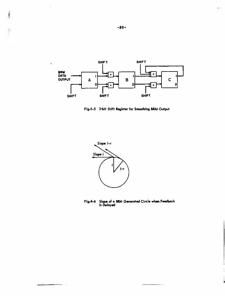
-89-
SHIFT SHIFT
9AMDATA I IOUTPUT A B
00
SHIFT SHIFT SHIFT
Fig.4-5 3"bit Shift Register for Smoothing BRM Output
Slope i-r
Slope
i-r
Fig.4-6 Slope of a BRM Generated Circle when Feedbackis Delayed
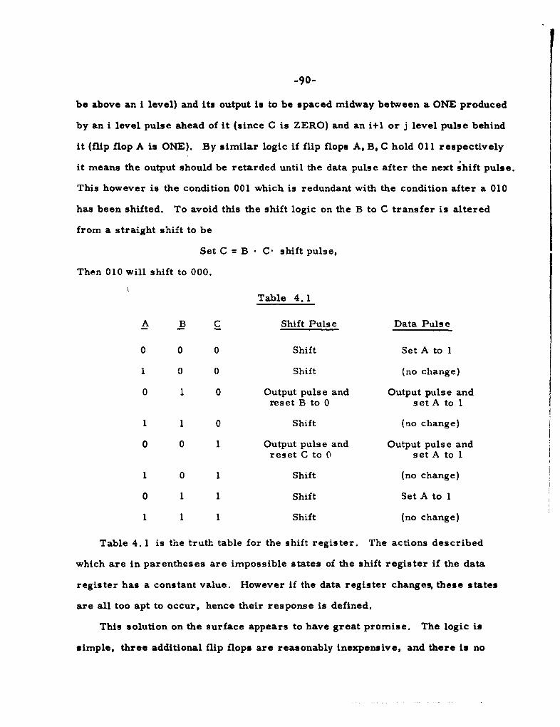
-90-
be above an i level) and its output is to be spaced midway between a ONE produced
by an i level pulse ahead of it (since C is ZERO) and an i+1 or j level pulse behind
it (flip flop A is ONE). By similar logic if flip flops A, B, C hold 011 respectively
it means the output should be retarded until the data pulse after the next shift pulse.
This however is the condition 001 which is redundant with the condition after a 010
has been shifted. To avoid this the shift logic on the B to C transfer is altered
from a straight shift to be
Set C = B C" shift pulse,
Then 010 will shift to 000.
Table 4. 1
A B C Shift Pulse Data Puls e
0 0 0 Shift Set A to 1
1 0 0 Shift (no change)
0 1 0 Output pulse and Output pulse andreset B to 0 set A to 1
1 1 0 Shift (no change)
0 0 1 Output pulse and Output pulse andreset C to 0 set A to I
1 0 1 Shift (no change)
0 1 1 Shift Set A to 1
1 1 1 Shift (no change)
Table 4. 1 is the truth table for the shift register. The actions described
which are in parentheses are impossible states of the shift register if the data
register has a constant value. However if the data register changes, these states
are all too apt to occur, hence their response is defined.
This solution on the surface appears to have great promise. The logic is
simple, three additional flip flops are reasonably inexpensive, and there is no
slow down in output rate except for the initial delay au the first pulse is moving
down the shift register. Unfortunately this is not the complete picture when we go
to generate curved lines.
Recall the basic equations for producing the circle
Xi=Xi-I + h Y i-1
Y = i-I " hXi- 1
Because of the delay introduced Xi is no longer h Y i-1 but is rather h Yi-r where
r is some number greater than 1 (minimum delay is 2 clock pulses) and which can
be quite large if Y is very small. Furthermore r varies with i. All in all the
mathmatics gets untractable. An easier way to view what is happening is to con-
sider in the case of circle generation that the feedback loop of VXi = h cos (ih) and
VYi = h sin (ih) is just the time rate of change or the slope of the curve at the
particular position occupied after i clock pulses. If a delay is introduced in this
feedback loop the VXi and V Yi are not the slope of the curve at the position
occupied after i clock pulses but are the slope at some earlier time. This means
the slope is not the tangent of the circle at time i but an earlier tangent which thus
has an axial component away from the center of the circle as can be seen in Fig. 4.6.
If the slope of a circle at time i-r is introduced as the actual slope at time i
(VXi = h cos (i-r) h) the curve will tend to be drawn out away from the center.
Thus a tendency toward an expanding "unstable" circle is to be expected in the
simulation of this system.
4. Simulation of the Smoothing Techniques
The results of this simulation are shown in Figs. 4.7 and 4.8. The first of
these is a photograph of three different circles (enclosed by a true circle for com-
parison purposes) produced by a BRM line generator incorporating the shift
register smoothing feature. These circles should be compared to Figs. 3. 7(a) and

-92-
(a) Radius 1628 (unstable
configuration)
(b) Radius 1628 (unstable
configuration)
(c) Radius 1438 (unstable
configuration)
Dot spacing expanded by two
Fig. 4.7 Circles, Generated by 7-Sit RMas with Shift Register"Smoothing" Added, Enclosed by True Circles for Coayorilon
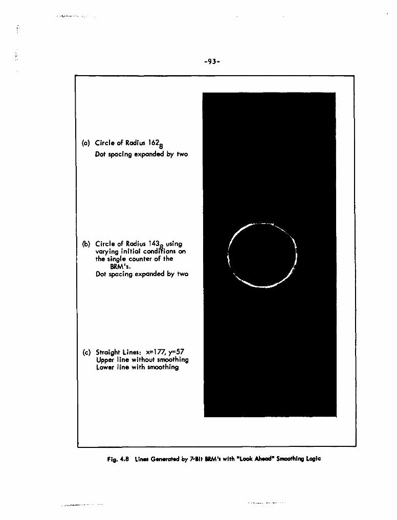
-93-
(a) Circle of Radius 1628
Dot spacing expanded by two
(b) Circle of Radius 143 usingvarying initial condiions onthe single counter of the
BRM's.Dot spacing expanded by two
(c) Straight Lines: x1 77, yl57Upper line without smoothingLower line with smoothing
Fig. 4.8 Lines Generated by 7-Bit IRM's with "Look AhWad" Smoothing Logic

-94-
3.8b)which illustrate the same circles generated by a BRM line generator without
the "smoothing." It is interesting to note that while the expected expansion of the
circle is not particularly evident, neither has the "smoothing" significantly
improved the closure or the unevenness of the figure. The principal effect of the
shift register seems to be that it changes the round-off errors, but does not reduce
them.
To eliminate whatever error might be caused by the delay of the shift register,
another version of the simulation program was written which performs the logic
required to produce the "smoothed" output directly from the state of the counter
and data register, (i. e. it simulates the logical Eqs. 26 and 27 and incorporates
the two flip flops suggested in section B. 2 of this chapter). Figure 4. 8) shows a
circle generated with this new program. No improvement is noticable. To examine
the "round-off" error, a multiple eosme was made of a circle of radius 1438 with
varying initial conditions on the single counter register. The results of this
experiment, Fig. 4. *), show no particular improvement over Fig. 3.9(b), the same
test given a BRM line generator without "smoothing."
The effect of the "smoothing"can be seen however in Fig. 4. 8c) where a straight
line generated by a conventional BRM is compared to the same line produced by
BRM's with the shift register "smoothing" feature.
The results of this study seem to show that the output pulse distribution can be
made more even and that this will show on the straight lines generated, but as far
as second order curve generation is concerned the smoothness of the change in x
and y is more of a second order effect and the real culprit is the round-off error.
C. ROUND-OFF ERRORS
1. Their Source
Ideally we would like to have a unit which is a perfect integrator to generate
curved lines. The equations of Chapter II were 1ased on this assumption. A per-
fect integrator with an input function y, shown in Fig. 4-8, will produce as an

-95-
output the exact area under the curve for any value of x.
The DDA varies from an ideal integrator in that it does not output the
exact area for any x, but rather a quantized version of the area, while it retains
the difference between the output value and the true value. Thus in a 3 bit DDA
an output occurs only after the area under y has attained at value 8. One output
pulse can be considered to have the weight of 8 area units. After 3 input clocks,
one output pulse has occurred (8 area units) and 7 is held in the R register (7
area units). The DDA has a round-off error then of 7 units. But since this
value is remembered, when more clocks are input these 7 units are applied
to the new quantities input. If y is to change value (as is shown at clock 4 in
Fig. 4.8) the DDA merely uses the new value of y to add to R, and it still
keeps track of the amount of round-off. This operation can be summed up in
the equations
S. =S. + y.+R.-R. 0> R.> R- iI • -x ai -
Si = 7,yj Ri + Ro
where S. is the output at clock time i, y. is the value of y at time j, and R. is
the value of the remainder at time j. Rmax in the example is 7 area units.
Unlike the DDA, the Binary Rate Multiplier has no memory of how much
round-off error it has produced. As was shown earlier this error is limited
to some Emax if y stays constant, but if y varies, the errors are accumulated.
The BRM relies on these accumulated errors averaging out. Thus in Fig. 4.8
the 3 bit BRM will produce a pulse on input clocks 1, 3, 4, 5, 6, 7 thereby
outputting six pulses. If these are again weighted by a factor 8 it means the
BRM emitted 48 units, while it only should have put out 44 units--an error of
plus four units. We can only hope that for the next series of input pulses it
will make an error of minus four units. The problem can be summed up in the
BRM equations:
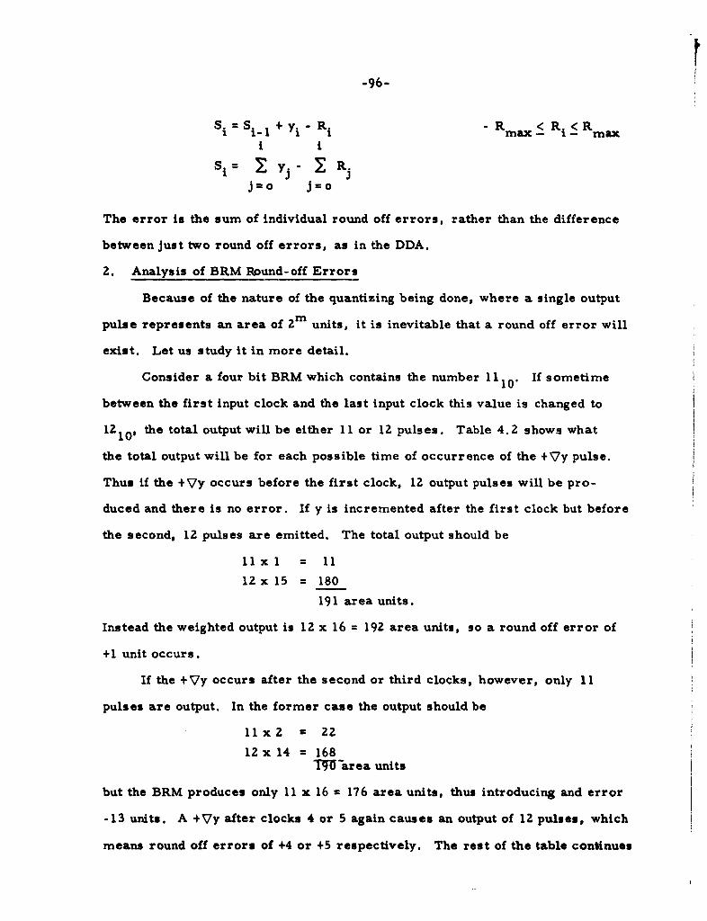
-96-
SiSii- + yi - Ri - Rmax-< Ri-< Rmax
i is i -- I yj - 2 R j
j1 Z 0 j= .j=o j=o
The error is the sum of individual round off errors, rather than the difference
between just two round off errors, as in the DDA.
2. Analysis of BRM Round-off Errors
Because of the nature of the quantizing being done, where a single output
pulse represents an area of 2m units, it is inevitable that a round off error will
exist. Let us study it in more detail.
Consider a four bit BRM which contains the number I I If sometime10"
between the first input clock and the last input clock this value is changed to
1210, the total output will be either 11 or 12 pulses. Table 4.2 shows what
the total output will be for each possible time of occurrence of the +7y pulse.
Thus if the +Vy occurs before the first clock, 12 output pulses will be pro-
duced and there is no error. If y is incremented after the first clock but before
the second, 12 pulses are emitted. The total output should be
11 x I = 1112 x 15 = 180
191 area units.
Instead the weighted output is 12 x 16 = 192 area units, so a round off error of
+1 unit occurs.
If the +Vy occurs after the second or third clocks, however, only 11
pulses are output. In the former case the output should be
11 x2 = 22
12 x 14 = 168'-area units
but the BRM produces only 11 x 16 = 176 area units, thus introducing and error
-13 units. A +Vy after clocks 4 or 5 again causes an output of 12 pulses, which
means round off errors of +4 or +5 respectively. The rest of the table continues
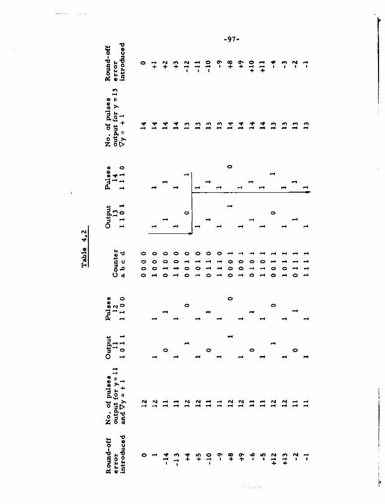
-97-
V u14V 0-4 N en r. -4 0 Oý O~ 00 CY%
0 0 + ++-- + + -4 aa
-4
4)-4
.41I
44
-4 - -4-4 -4
24 '. 44 . 4 -4 -4 4 -4 4
4J -4 -4
00
.444
0 0
0 0 1 --4 -4 -4 +4-
N-4

-98-
in this manner. It is interesting to note that if the data register is being decre-
menited (i.e. contains 12 and a -Vy reduces it to 11) the round off errors intro-
duced are of the same magnitude, but of opposite sign, as occur when y is incre-
mented. Note also that the "number of pulses output" column alternates bet-
ween 12 and 11 at the same time as bit b of the counter changes state. Table
4. 2 also shows the output for the BRM when the data register contains 13 and
a +Vy pulse is introduced. In this case the "number of pulses output" column
alternates in synchronism with bit c of the counter.
If one produces a similar table for any other value for this BRM some
facts become evident. When a single step occurs in the data register, some
round-off error is always introduced, unless it occurs before the first clock.
The sign and magnitude of this round-off can be ascertained by considering the
value in y, the counter state, and the direction of the step (increment or decre-
ment y). To determine the sign of the error find the most significant bit of the
data register which changed state due to the step. Examine the state of the
corresponding counter bit. If these two bits are the same (both ONE or both
ZERO), the round-off error introduced will be negative. If they differ, the
round-off is positive.
Consider as an example, a transition from 13 to 14 occurring between
the fourth and fifth clock pulses. Three output pulses will result from the first
four clocks when the data register contains the value 13. Ten more pulses will
be output from the remaining 12 clocks during which time the data register con-
tains the value 14. The total number of output pulses is 13, as we can see in
the table. This introduces a round-off error
13 x 16 - (13 x 4 + 14 x 12) = 208 - 220-- - 12 area units.
The sign of this round off can be quickly determined by looking at bit 2 of the
data register after it has been stepped (the most significant bit to change as a
result of the step) and compare it to bit c of the counter (the corresponding bit of
-99-
the counter). Since both bits are ONE the round-off error is identified as
negative, which checks.
Note that no error is introduced by the changing of the data register
itself. Only after the BRM produces output pulses are there errors. But
the state of affairs in the data and counter registers at the time of altering
the data register establishes what the errors produced by output pulses will be.
The magnitude of the error is determined by observing the state of
the counter, the sign of the VX pulse and the sign of the round-off error.
If the sign of the round-off error and the sign of VX match, the value of the
contents of the counter is the amount of round-off. If they differ, the contents
of the counter is the two's complement of the amount of round-off error.
Unfortunately this is not the entire story when considering the BRM as
we intend to use it. In our application the data register does not change
by only a single unit for each 2 input clocks. This means that each pulse
output must be weighted by an appropriate round-off factor, based on the
magnitude of round-off error introduced by each preceding Wy pulse.
It soon becomes obvious that to properly apply any round-off error
correction factor, we must accumulate and store the magnitude of the
round-off as we go along. The only way to do this accurately is to provide
a register 2 m bits long. But this leads us right back to the DDA which with
its data register and remainder register is the simplest arrangement of these
two registers for producing both a smooth and correct output.
Despite the validity of the above statement, several attempts were made
at simulating equipment that would reduce the round-off errors. It was hoped
that by storing less than 2m bits some sort of rough cut at the round off
error could be made. To date no significant improvement has been made.

CHAPTER V
HARDWARE CONSIDERATIONS
A. GENERAL
The intent of this study has been to examine specialized computing
equipment to improve a present day digital computer display system. The
motivation has been the immediate need for such equipment in Computer-
Aided Design. It has become apparent that before significant progress
can be made in this field a better display system will have to be constructed.
With this immediacy of purpose in mind, the philosophy adopted in this
study has been to design the system from off-the-shelf components. Also
since a machine of this nature is likely to be mechanized, the cost is of
vital interest.
The two considerations of time and money dictated to a large extent
the direction taken by the study. For example they prompted the extended
research into the .Binary Rate Multiplier, which though obviously a poorer
computing device than a DDA, could be made more cheaply and perlaps
with proper alteration could be made to give satisfactory results. Mixed
digital-analog computing techniques were discarded for essentially the
same reasons. Although with improved components and considerable
engineering effort it is quite possible these techniques could be competitive,
the state of the art does not support building this system with such schemes
today.
The general characteristics of digital computer display scopes of
today were obtained from conversations with several manufacturers of such
scopes (Digital Equipment Corporation, Burroughs Corporation, Transdata).
-101-
-1OZ-
To get the large working surface desired (10 inch x 10 inch minimum
active area) without losing resolution of the points, magnetic deflection
coils were recommended. Scopes using tnese coils do not respond as
rapidly as scopes employing electrostatic deflection, but movement
of several grid points distance each microsecond is well within the
state of the art. Based on this and on estimates of the amount of data to be
displayed, it was decided that a reasonable plotting rate to achieve would
be one megacycle, i.e., a new point each microsecond where each point
is no more than one horizontal increment (1/1 0 0 th incli and one vertical
increment distant from the previous point. This would allow plotting to
occur about 100 times faster than can be done on the IBM 780 Scope Unit.
So far no mention has been made as to how the computing devices
discussed should be built. There are two general classes, serial and
parallel, and a myriad of basic circuit elements to choose from; transistors,
tunnel diodes, wired magnetic cores, sonic delay lines, electronic delay
lines, etc. In view of the philosophy adopted however it seemed prudent to
pick the most straight forward way to do the job. With this in mind it
was decided to examine the potential of the pluggable digital building
blocks manufactured by a number of companies, and consider parallel
computation.
The choice of parallel operation over serial was based on the one
megacycle output rate desired. To make a serial DDA or BRM with this
output rate would entail use of very high speed circuitry, which is expensive
and not easy to work with. It was felt that this would not be in keeping
with the proposition of using cheap, off the shelf hardware.

-103-
The particular line of hardware to be used in actual construction
is a decision to be made when a system design for a machine is completed.
However to ensure that the system proposed here was not entirely out of
touch with reality, the author chose to breadboard a working model of the
fundamental logical blocks specified in the thesis.
The circuit blocks chosen were those made by the Digital Equipment
Corporation (D.E.C.), who have three complete lines of circuitry; 10
megacycle, 5 megacycle, and 500 kilocycle. The basic storage element
in all these lines is the bistable flip-flop. The triggering of these units is per--
formed by pulses which are normally gated by standard level logic. The pulses
required for the 10 megacycle circuitry are 40 nanoseconds wide; for
the 5 megacycle logic they are 70 nanoseconds; and for the 500 kilocycle,
400 nanoseconds wide. Despite this discrepancy, there are techniques for
marrying circuits of different types into the same system. Thus high
speed circuits need be used only where they are required by the signal frequency.
For example a 10 bit unidirectional counter which is incremented at a 4
megacycle rate need only have the first three stages be 5 megacycle type
circuits. The fourth stage of the counter can be driven at a maximum rate
of 500 kilocycles and can thus be of the slower (and cheaper) line of
equipment. It turns out that the D.E.C. 500 kilocycle flip-flop when
used as a counter (complement input) will actually operate at I megacycle,
so in actual fact only the first two such stages need be of the faster variety
of hardware.
B. THE BASIC 1 MEGACYCLE BRM
Figure 5. 1 illustrates the first unit to be breadboarded, the
basic 1 megacycle BRM. The diagram of Fig. 5.1 is in the standard

-104-
igi
14g
hiL InLL Af -
crIwI

-105-
symbology of D.E.C. logic. A brief glossary is given with the figure,
but for a more complete explanation the reader is referred to the D.E.C.
logical handbook. 8
The unit was built principally to prove its feasibility and to study the
resynchronizing problems. Re synchronization is necessary for the
rotation matrix BRM outputs in order to keep the h and v accumulating
registers as simple counters. There are three inputs to these registers
each of which may be plus one, minus one, or zero. Due to the delays
inherent in the BRM the outputs may occur at any time from 100 nanoseconds
to 500 nanoseconds after the initiating clock pulse, depending on the pulse
rate into each BRM and the value they contain. Only if the outputs are
made coincident with the basic clock can the output times be predicted
accurately. Once this synchronizing has been accomplished, the output
pulses can be applied through different fixed delays to provide three
separate pulses spaced at 200 nanosecond intervals. The least significant
stages of the h and v registers are then 5 megacycle flip-flops which will
accept pulse inputs at this high speed. By this contrivance the outputs
of three rotation matrix BRM's are added into a single register.
The breadboard model was made up for the most part from 400 Series
(500 kilocycles) flop-flops, excepting the resynchronizing flip-flops and
the single output flip-flops which simulates the least significant bit of
the h or v counter.
-106-
The logical element used to gate the 0 to 1 transitions is the
capacitor diode gate. This gate has two inputs, a level input and a
pulse input. On the pulse input is a 330-micromicrofarad capacitor which
will differentiate a negative going level input and provide a pulse at the
transition time. The outputs of six of these gates are tied together into
a one transistor inverting amplifier (PI). The output of this amplifier
feeds the input to the resynchronizing flip-flop directly on the reset side.
This flip-flop is normally in the ONE state. Its being set to the ZERO
state permits a clock pulse through a gate (Gate R) to drive a pulse
amplifier (Output P.A.) which sets the resynchronizing flip-flop to a ONE
again and provides the output pulse of the BRM. By this technique the
output pulses of all the BRM's are resynchronized to the basic clock.
To investigate potential problems in summing the outputs of
several I megacycle BRM's into a single counter stage, the synchronized
outputs of BRM x and y of Fig. 5.1 were used to drive a single 5 mega-
cycle flip-flop which simulated the least significant bit of the counter.
The summation was accomplished by delaying the output of the y BRM
by 200 nanoseconds, while not delaying the x BRM at all. If there were a
third BRM, its output would be delayed by 400 nanoseconds. This scheme
worked very satisfactorily. Figure 5.2 illustrates the output of this BRM
pair and the first stage of an accumulating register for 64 input pulses.
Part (a) is the output of the x BRM which contains the value 34. Part (b)
is the output of the y BRM containing the value 8. Part (c) is the first stage
of a counter which is being triggered by the sum of the two pulse trains
(a) and (b).

-107-
(a) x BRM output = 34
(b) y BRM output = 8
(c) First stage ofAccumulating Register
0 20 40 60. SEC
Fig. 5.2 Output of 1 mc Dual lM for One Cycle of 64 Input Pulses (lower trace).Upper Trace Is mrst Significant Bit of ERM Counter

-108-
C. "SIGNED" ACCUMULATING REGISTOR INPUT LOGIC
In the final design of such a system, the above breadboard model for the
adding of pulse trains is a bit inadequate, since no provision has been
made to identify the sign of the pulse, i.e. whether it should increment or
decrement the register. Figure 5.3 however shows the logical diagram of
a simple solution to this difficulty. The output pulse of each BRM is fed
into two pulse amplifiers through gates controlled by the sign of the BRM.
Thus one amplifier is activated by positive pulses, the other by negative
pulses. The positive pulse amplifier drives UP counter logic, the negative
pulse amplifier drives DOWN counter logic.
This leads us into the difficulty of what to do if the input
pulses oscillate between plus and minus pulses at a rate above 1 megacycle,
i.e., if at each input pulse time there is both a positive and negative output
pulse. The lower order stages of the h and v counters are made from 5
megacycle circuitry, but the more significant bits are not. Unfortunately
when one of these counters contains the binary value 0111111111 and the input
oscillates between +1 and - I at more than I megacycle, the + 1 pulse
causes the counter to switch to 1 000 000 000 and the - I pulse makes it switch
back to 0 111 111 111. Thus all the bits up to the tenth are forced to operate
at a frequency above I megacycle. Unless a way to prevent such an
occurrence can be put in the system, all the flip-flops of the h and v counters
must be of the 5 megacycle variety.
There are several ways around the problem. One is a scheme we
have already discussed but for other reasons. This is the "Backlash Unit".
It filters out the high frequency oscillations. Since there are three sources
of input however, a two stage Backlash Unit is required. The two stage unit
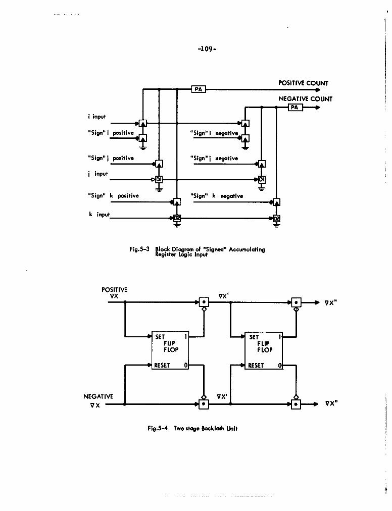
-109-
POSITIVE COUNT
NEGATIVE COUNT
i input
"Sign" i poitive "Sign" i negative
"Sign" j positive "Sign" j negative
input D1
"Sign" k positive "Sign" k negative
k input
Fig.5-3 BIock Diagram of "Signed" AccumulatingRegister L.gic Input
POSITIVE
SET I SET ISFLIP F LIPS FLOP FLOP
0 RESET 0 RESET
NEGATIVE VX,
VX 7X"
Fig.5-4 Two stage Backlash Unit

-110-
is diagrammed in Fig. 5.4. To output a positive pulse, both stages
of the unit must be ON, while to output a negative pulse both stages
must be OFF. The other plan is to store the three input pulses in a
separate two bit register which is then added directly into the accumulating register
in one operation with adding logic. Since the number can be at most 3, the higher
order bits made of slower circuit types can be at most incremented by a carry
pulse.
D. HIGH SPEED COUNTERS
Inherent in the entire design philosophy of this display system has been
the assumption that a near 1 megacycle pulse rate can be maintained.
Although this in itself is not a difficult task for the present state of the
art, it is not done cheaply. The price differential between 500 kilocycles
circuitry and 5 megacycle circuitry is considerable, on the order of two
to one. To operate at 1 megacycle a DDA must complete a full add in 1
microsecond. For a BRM it requires a counter that will operate at a
megacycle.
This introduces a further economic advantage for the BRM over a
DDA. To provide a parallel DDA which is capable of a full add in one
microsecond requires the entire R register to be made of 5 megacycle
circuitry since a full add takes two steps to complete. The BRM on the
other hand, at 1 megacycle can be made entirely of 500 kilocycle flip-
flops which complement at the higher rate of I megacycle.
The nicest feature of counter logic over add logic is that as
long as the count moves in one direction, higher order bits switch at
respectively slower rates. Thus even at input rates above I megacycle,
the more significant bits of the counter switch at a more leisurely pace.
This makes it feasible to consider using BRM's above I megacycle as the
basic line generator.
-111-
The limiting factor on the counter illustrated in Fig. 5.1 is the
carry propagation time. For the Type 4215 flip-flops used in this
model this time is 50 nanoseconds per stage. This would presumably limit
1000the length of counter to ZD O 20 stages. In itself this appears fast
enough, but when considered as a part of a BRM with feedback as required
in curve generation, there are more timing problems to consider than
just propagation of the carry. For a curve-producing line generator,
in the 1 microsecond between clocks the logic must be fast enough to do
the following tasks: the m bit counter must propagate its carry to the
last bit (mx 50 ns), the capacitor diode gate must generate a pulse
(50 ns), this pulse must be amplified through a pulse amplifier (25 ns)
and fed back into the least significant digit of a date register, which in
turn must be able to propogate its carry to the far end (m x 50 ns), the
last stage must switch state and change the condition of the first stage
pulse gate (1 microsecond), all within 1 microsecond. Neglecting the long
capacitor diode gate switching delay, this infers a maximum register length
ofM = 1000 - 50 - 25 9 stages
But to give reasonable variation in circle sizes, the line generator should
be at least 12 bits long. Furthermore the slow reaction of capacitor
diode gates to changes in the level input implies that they must be abandoned.
To speed up the counter, look-ahead logic may be incorporated.
This scheme is illustrated in Fig. 5.5. Note in this block diagram that
flip-flop A4 is not activated by the carry from stage 3 but instead is
pulsed by the basic clock through a gate which allows the pulse only when
flip-flops A 1 , A 2., and A 3 are all ONE. This is the time flip-flop A4 is
normally incremented by the carry pulse, but it now does not need to
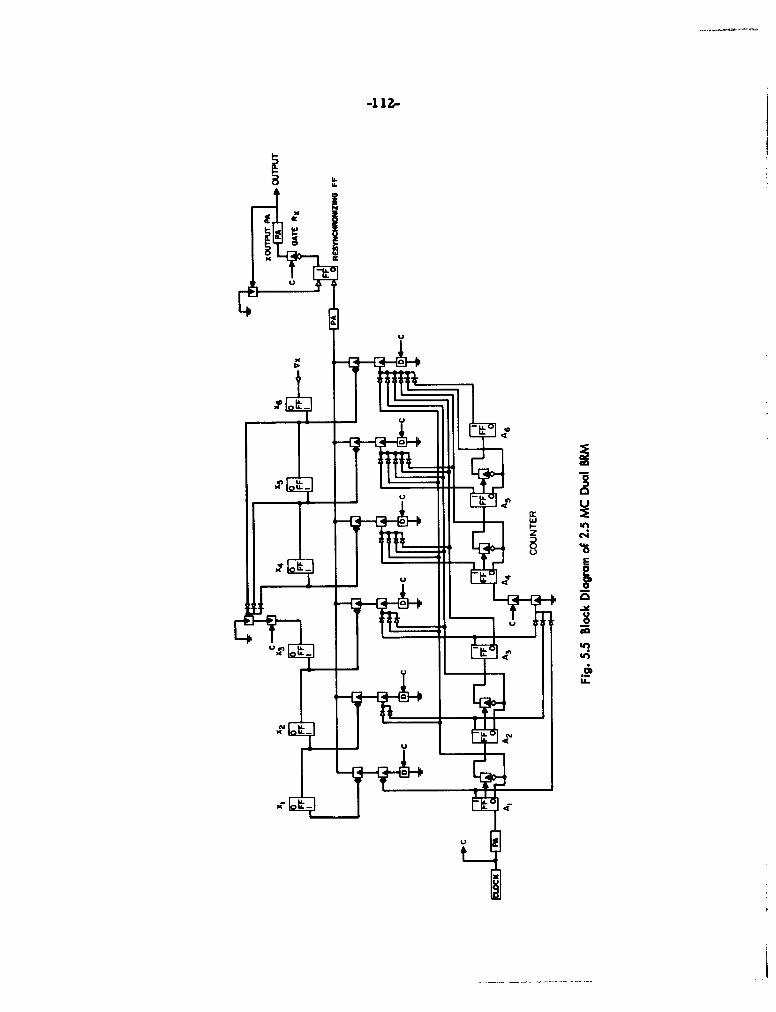
-lii-
z 1
-0
00
tt,
tt - IY

-113-
wait the 150 nanoseconds for propagation since the basic clock provides the
pulse source. This same design can be used several times throughout the
counter, but there is one subtlety to be watched for, however. Stage 1 must
not trigger too fast after the clock appears or else it will change the state
of the AND gate before stage 4 can trigger. This can he ensured by using
flip-flops in the counter which delay changing state until after the clock which
changes them has gone away. For the 500 kilocycle circuitry this delay is
400 nanoseconds.
Based on the above method for speeding the counters it is reasonable
to assume that the total delay in either counter (BRM counter or data
register) can be kept under 250 nanoseconds. The capacitor diode gates
can be replaced by standard gates based on similar logic. The delay
through such logic, (from direct measurements), appears to be well under
50 nanoseconds, and through a pulse amplifier Z5 nanoseconds. It seems
safe, then, to assume that a I megacycle BRM of 12 bit length is entirely
feasible.
From the results of Chapter III, we saw that a BRM gives unsatisfactory
second order curves, but BRM generating a figure four times as big and
then divided back down by four is acceptable. But this makes the plot four
times as slow. If the BRM line generator could be made to operate
four times faster without costing more than the DDA, it still would be the
preferable device. Based on the figures given above it seems questionable
if a factor of four increase could be made.
The apparent limit is 2.5 mc using mixed circuitry. This is because look
ahead logic must be incorporated to speed up the carry propagation, but this

-114-
(a) x-5
(b) x 59
(c) x 4 1
Fig. 5.6 Output of 2.5 mc Single ORM for One Cycle of 64 Input Pulses (lower trace).Upper trace is most Significant lit of IRM Counter
-115-
ruires flip-flops which do not change output state until 400 nf after they
have been complemented. Thus they can not control the gating logic for
the next pulse properly for 400 nf. A faster input clock could cause errors.
In order to get true 4 megacycle operation it appears the line generator
must be made of 5 megacycle hardware. The design of this unit would
be very much like that of the 1 megacycle BRM except for the speed of the
elements and use of static logic in place of the capacitor diode gates.

CHAPTER VI
OTHER STUDIES
A. GENERAL
The study of the design of a system for generating axonometric pro-
jections of three dimensional figures led to some conjectures about a
system for providing other projections; notably perspective and stereo-
scopic. The intent would be that the computer supply the same basic
information to the display system (line information in an absolute x,
y, z coordinate space) and the computing equipment in the display unit
would perform the necessary operations to generate the appropriate pro-
jected display.
Unfortunately time did not permit a very thorough investigation of the
problems involved in these projections, but systems for generating these
displays were simulated and the results are reported below.
B. STEREO PROGRAM
First let us consider the nature of the stereoscopic projection. Figure
6. 1 is a top view of a pair of eyes, which are a distance e apart and D
units from the two dimensional picture plane, looking at two points A
and B which have identical x, y coordinates, but A is on the display screen
surface while B is z units behind the surface. The right eye will see
B at the position BI on the viewing screen while the left eye will see B
at B". In Fig. 6.1 the triangle RCB is similar to B'AB. Thus
e/2 = B-(2)D+z z
-117-
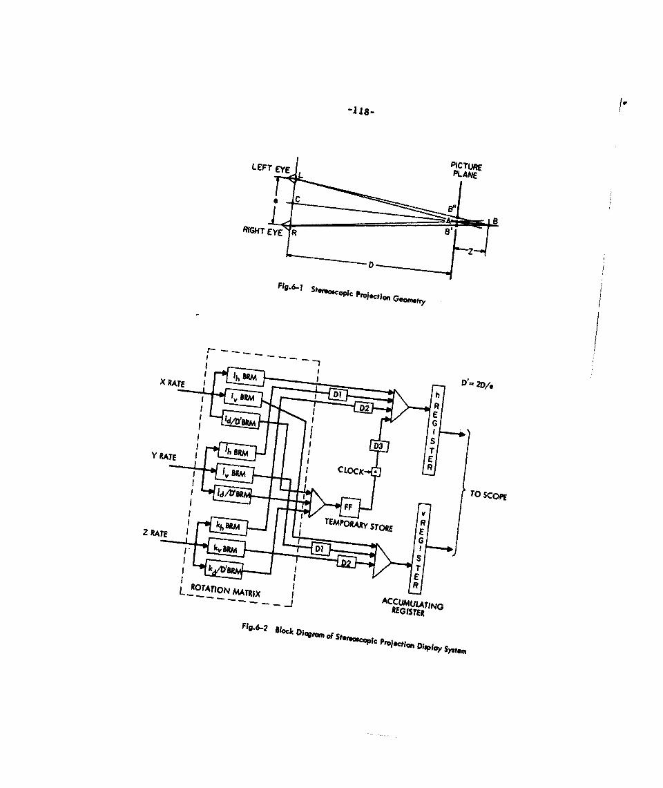
LEFT EyE PICTUREPLAINRE
0 C
zRIGHT YE fi
-----------_L erftftoo
Mro~cio
RG*OnwtIN
Xl c R A T If 2 D/pc u y s e
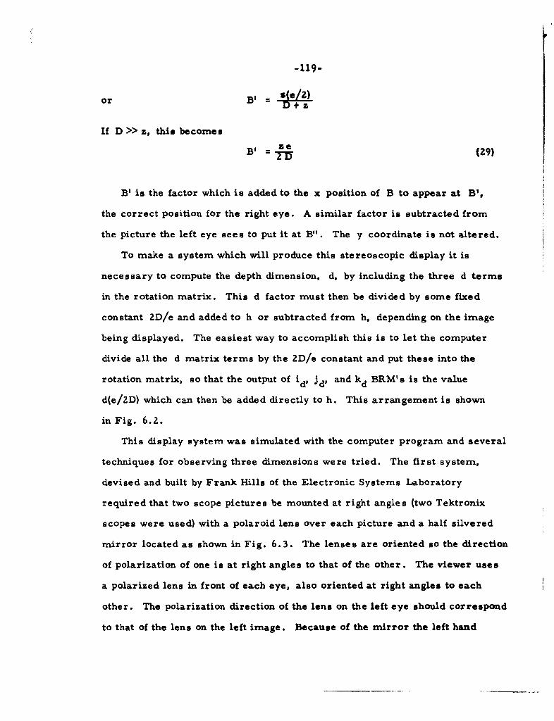
-119-
or BI =
If D >> z, this becomes
B' = Ze (29)
B' is the factor which is added to the x position of B to appear at B',
the correct position for the right eye. A similar factor is subtracted from
the picture the left eye sees to put it at B". The y coordinate is not altered.
To make a system which will produce this stereoscopic display it is
necessary to compute the depth dimension, d, by including the three d terms
in the rotation matrix. This d factor must then be divided by some fixed
constant 2D/e and added to h or subtracted from h, depending on the image
being displayed. The easiest way to accomplish this is to let the computer
divide all the d matrix terms by the 2D/e constant and put these into the
rotation matrix, so that the output of id' id' and kd BRM's is the value
d(e/2D) which can then be added directly to h. This arrangement is shown
in Fig. 6.2.
This display system was simulated with the computer program and several
techniques for observing three dimensions were tried. The first system,
devised and built by Frank Hills of the Electronic Systems Laboratory
required that two scope pictures be mounted at right angles (two Tektronix
scopes were used) with a polaroid lens over each picture and a half silvered
mirror located as shown in Fig. 6.3. The lenses are oriented so the direction
of polarization of one is at right angles to that of the other. The viewer uses
a polarized lens in front of each eye, also oriented at right angles to each
other. The polarization direction of the lens on the left eye should correspond
to that of the lens on the left image. Because of the mirror the left hand

-120-
RIGHT IMAGE
__.......... POLARIZED LENS
LEFTIMAGE
IHALF SILVERED MIRROR
POLARIZED LENS
! • POLARIZED LENSES
LEFT EYE RIGHT EYE
Fig.6-3 Stereoscopic Viewer using Polarized Lenses
______ LEFT IMAGE RIGHT IMAGE
SCREEN
-MIRO
LEFT EYE RIGHT EYE
Fig.6-4 Stereoscopic Viewer using a Single Mirror
- 1Z1-
image must be plotted as the mirror image, rather than the true left
eye image.
The resulting pictures were quite good, and the three dimensional
effect was easy to see. The principal objections to the viewing system
were the difficulty in aligning the two scopes with each other and the
inability to work on the picture directly with a light-pen.
The second scheme was very simple but produced surprisingly satisfactory
results. This required the two images to appear on the regular display
scope, with the left image again a mirror image and displaced from the right1
image in the horizontal direction about -1 the scope width. A single full-
surfaced mirror is placed midway between the two views as shown in
Fig. 6.4. The viewer than places his head so his eyes are on opposite sides
of the mirror and he looks at either image. Figure 6.4 shows how while
looking at the right image, the left eye actually sees the left image. With
very little effort these images can be superimposed and a three dimensional
effect results.
This system is crude since it requires the viewer 4o keep his nose
virtually touching the mirror, but it is simple, requiring almost no
alignment, and allows light-pen work to be done directly on the scope.
Figure 6.5 shows two objects which were produced by the stereo
simulation program. The picture shows how the computer scope looks for
this display. Figure 6.6 is an expanded view of the tetrahedron of Fig. 6.5.
The three dimensional effect can be observed in this figure by placing a
mirrored surface between the views and looking at it in a similar manner

-122-
(a) Tetrahedrons
(b) Spheres
Dot spacing not expanded
Fig. 6.5 Left and Right Images of Stereoasepic Projections

-123-
Right Image
Left Image
Dot spacing expanded by two
Fig. 6.6 Expansion of Images of Stereoscopic Prolectiors of Tetrahedrons

-124-
to that diagrammed in Fig. 6.4. The crudeness of lines in Fig. 6.6 is
worth noting. It is more ragged than the standard axonometric projection
of Chapter III as is to be expected, since the addition of the depth term
is a further source of fluctuations.
C. PERSPECTIVE PROJECTION
Another possible useful display is the perspective projection of a three
dimensional object. Although this is not the projection familiar to drafts-
men, it has the one advantage of giving an illusion of depth to the observer.
Thus it is easier to identify which surfaces are behind which. However,
the figure is distorted to give this illusion. Thus parallel lines do not
plot as parallel lines and lines of equal length are not shown equal if they
are at different depths.
The perspective projection can best be analyzed with the aid of Fig. 6.7.
In this figure we wish to determine the coordinate value of y' which is the
perspective projection of the point y which is at a depth z from the plane
of the picture. The triangles EAB and EA'B' are similar so that the
following ratio holds:
(30)
Thus DYThs Y ( ) = Y(1 +ziD) (31)
This equation is a bit difficult to mechanize, but it can be simplified
if we make the assumption that D >> z. Then we can expand 1/(1 + z/D)
into a Taylor series and neglecting the higher order terms:
y = y(l - z/D+z 2 /D2 . . ....
y y(l - z/D) (32)
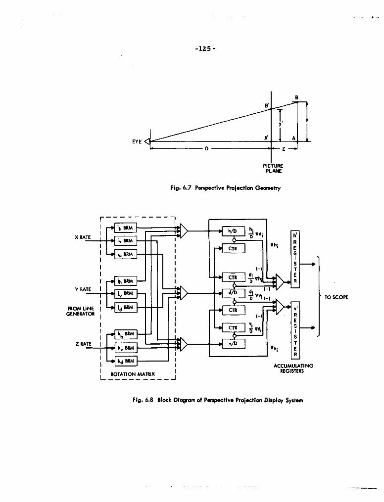
EYE I A
PLANE
Fig. 6.7 Perspective Projection Geometry
IT SCOP!M
X LRROTATION BR MATRI RGITR
Fig.~~CT 6. lc igamo esetvePoeto isa SsEm
-126-
An identical relation for the x coordinate can be obtained if no
attempt is made to include stereo projection as well.
The mechanization of this equation into hardware is more difficult
than the stereo display, since the z factor is multiplied by x and y
rather than just added directly. Considering our display system with its
rotated coordinate system, the x, y, z of the above equations become
h, v, and d. Taking just the y coordinate, our equipment must evaluate
the following equation:
v' v(l -d/D)
In terms of difference equations this becomes
v -idi di viWit = W i -V -- DW i ' " - f i " -U V d i
Figure 6.8 outlines the block diagram of the required system to perform
this operation for h and v. The vertical component is generated from the
axonometric vertical component with two terms added; one to account for
changes in the vertical with the depth constant, the other for changes in
depth with the vertical constant.
A version of the simulation program was written which generated this
display to examine the quality of the picture, illustrates the results. Figure 6.9
(a) and (b) show a block with a hole through it in perspective while part (c)
is an axonometric view of block in the same orientation as (b). It can be
seen that lines on the perspective projection are very ragged and that so
much error has been introduced that the figure does not properly close.
Time did not permit a thorough study of the source of this error but it
is believed to be the accumulation of round-off from the various computing
elements plus a computation error due to the simplifying assimptions made.
A combined stereo-perspective display can also be generated. Its
analysis is done in a manner similar to those already shown. The hard-
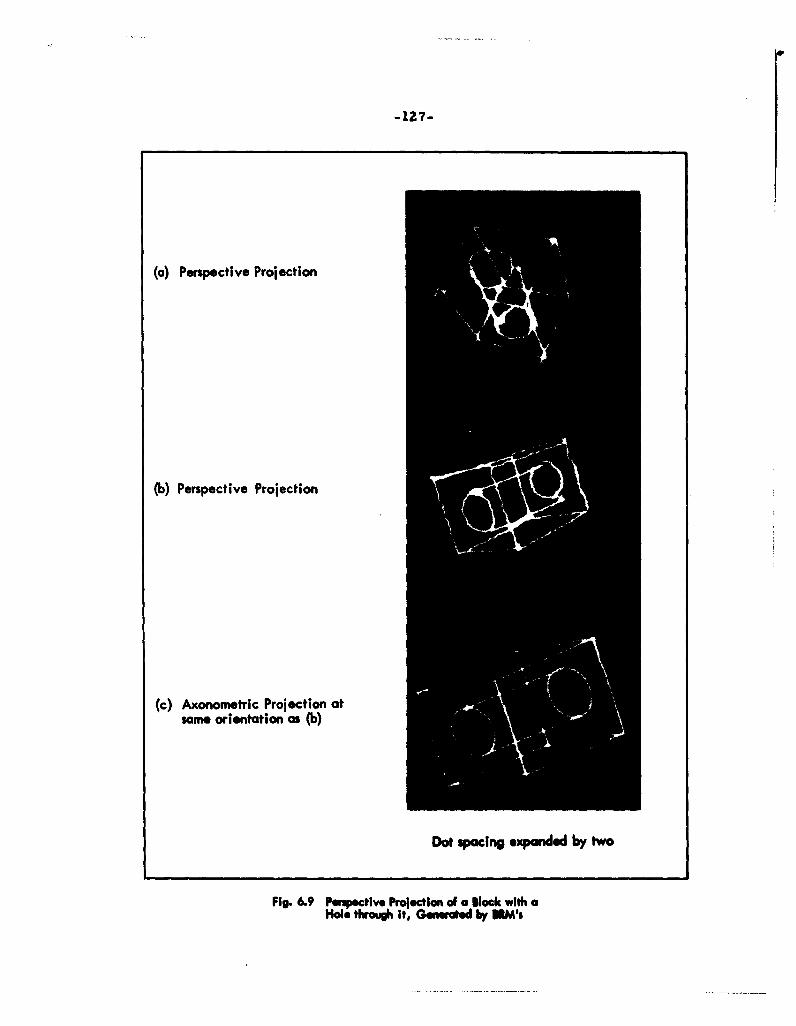
(a) Perspective Projection
(b) Perspective Projection
(c) Axonometric Projection atsame orientation as (b)
Dot spacing expanded by two
Fig. 6.9 Pempective Projection of a lock with aHole through it, Gamnsed by DIM's

-128-
ware required to produce it is a combination of that required for the
two projections separately. No simulation was attempted for this system.
D. CONCLUSIONS
Either perspective or stereoscopic display projections or both can
be built into special purpose computing hardware to relieve the computer
of necessary computations to generate the display. The picture quality
however becomes rather crude and the amount of equipment required is
considerable. To improve the quality of the display, about all that can
be done is to compute to more accuracy and disregard the least significant
bits. In incremental computation this means a slow down in display speed.
Note that except for this there is no slow down in the display caused by
the introduction of perspective or stereo computing equipment.
The expense involved for all this added hardware can only be justified
if the projections are to be the principal modus operandi of the display
system. There is considerable question about this, however. For this reason
it does not seem worthwile to pursue these more sophisticated aspects of
the display problem at this time. A nice feature of this system is that it
is expandable to include perspective or stereo display in the future, without
altering the basic units of the line generator or the rotation matrix, so that
extension of the system to include these secona order improvements is quite
simple.
CHAPTER VII
CONCLUSIONS AND RECOMMENDATIONS
A THE PROBLEM AND THE SYSTEM SOLUTION
In Chapter I it was shown that there is an immediate need for an improved
display system for the Computer-Aided Design studies being done at the Electronic
Systems Laboratory. The principal requirements for the new system are to increase
the plotting speed over the present point-for-point computer scopes by several
orders of magnitude, and a similar reduction in computer time required to generate
these points. Since the prime use of this system is for design of three dimensional
shaped objects, aids for calculation of the two dimensional projection of these
three dimensional figures are of considerable value. In addition it is desirable
that provision be made for simple computer operations to rotate, translate or
expand the view.
A system is proposed which provides straight line and second order curve
generation by transforming input parameters into appropriate pulse rates which
drive the scope unit. These techniques improve plotting speeds by a factor of from
10 to 100, but the data rate provided is still less than is ultimately desired. The
limiting factor is the state of the art of the display scopes of today. But since
significant work in Computer-Aided Design can be accomplished with even this
initial increase in speed, it is important to build a unit based on the present
commercially available hardware now.
The proposed system also contains provision for computing the two dimensional
axonometric projection of three dimensional input information. This is accomnplished
by including the z axis in the line generator and providing a Rotation Matrix after
the line generator, which accepts the x, y, z data rates and outputs two of the rotated
-129-
-130-
coordinate axes, h and v to the scope. The Rotation Matrix, in addition to
providing the transformation from three dimensions to two, permits the second
order curve portion of the line generator to be much simplified.
Other features of the proposed system are h and v accumulating registers
which can store numbers which are several bits larger than the minimum scope
deflection and a Sense Line back to the computer which identifies when the display
is entirely off the screen. These features assist the computer in the problem of
determining the "edge" of the displayed region.
The system proposed in this thesis is not just one display system, but a whole
family of possible systems. The basic two dimensional vector generating unit
(which processes only x and y data with no feedback) plus the basic accumulating
registers constitute the simplest system, which is capable of producing just
straight lines. If a Rotation Matrix consisting of four Binary Rate Multipliers
is included and more logic is added to the line generator, the resulting machine
is capable of producing straight lines or any second order curves in two dimensions,
and as such meets the minimum requirements for increased speed and versatility
for the Computer-Aided Design program.
This basic machine can be augmented in several different ways. If extra bits
are added to the h and v registers and a Sense Line back to the computer is
added, the "edging" computations can be reduced considerably for the Central
Processing Unit. In a different vein, for a rather small investment the three-
dimension-to-two-dimensional-axonometrix-proje ction computation can be
incorporated into the system. More complex systems beyond this such as the
perspective projection, stereo projection, automatic light-pen tracking and exact
"Wedging" are further variations on the same basic machine. These last two
features are discussed later in this Chapter.
-131-
B THE BASIC ELEMENT FOR THE LINE GENERATOR
A good portion of this study has been devoted to the question of whether to
use the DDA or the BRM as the basic element for the line generator. The DDA
gives better performance, but costs more if parallel computation is considered.
If serial computation is chosen, the DDA is clearly superior since the logic for
a serial DDA is as simple as for the BRM. But as mentioned earlier, serial
computation for the speeds required is more expensive than parallel computation
and involves reliance on newly developed circuits. For parallel computation, the
case is quite close between the DDA at 1 megacycle and the BRM running at 4
megacycles and reduced back down to 1 megacycle (thereby achieving four times
the accuracy and giving performance comparable to the more sophisticated DDA).
If further study into the round-off error problem of the BRM provides a significant
improvement in its operation, it may well be the preferable unit. In any case a
final decision must be based on a precise cost evaluation cf each system. No such
evaluation was attempted in this study.
C MORE SOPHISTICATED PROJECTED DISPLAYS
Chapter VI indicates that projections of the three dimensional figures which are
more sophisticated than the axonometric projection can also be produced by
specialized equipment. Stereoscopic projection and perspective projection were
simulated. The results, however, were not entirely satisfactory using straight-
forward techniques. A different scheme which bears study is modulation of the
spot intensity to give an illusion of depth. More investigation is required before
any workable system can be proposed, so that it does not appear worth designing
such a system at this time. After a simpler system has been in operation and an
evaluation has been made of the usefulness of various types of projections and
displays, the need for a more complex unit can be re-evaluated. If it is justified
by this research, the necessary logic may be added to the existing system as a
modular package.
D OTHER POTENTIALS OF THE SYSTEM
We have considered in this work only the display problem itself and how it
can be reduced. An associated problem which has not been mentioned is the
large amount of computer time involved in light-pen tracking. The proposed line
drawing display system lends itself well to eliminate this problem entirely. As
suggested by Randa, automatic pen tracking is not difficult to add to the console
system, once a vector generator is available. If logic is included to compute the
center of the pen's field of view and to transfer this information back to the
central processer, it will remove a tremendous load of trivial computations from
the computer. The best way to perform automatic pen tracking is not entirely
clear and represents an excellent field for further study.
If pen tracking is automated, another aid to the computer becomes quite feasible.
Since the coordinates of the pen location will have to be transferred to the computer,
it seems entirely reasonable to use this same transfer in combination with the
oversized accumulating registers to accomplish precise "edging" for the computer.
One plausible way of accomplishing this is to have the display system halt whenever
the display goes off the screen and interrupt the computer. On the first pass
through the display the CPU would output the entire display. Whenever it is
interrupted, the computer would read in the states of the appropriate registers
(h, v or x, y, z) to determine the "edge". Then the system would be released
to continue processing the data till the figure comes back onto the scope face, at
which time it again would stop and give the computer the coordinates of this new
point. All portions of the display file which were off the scope edge would be
omitted from a "reduced display list". This reduced list is then used for the
succeeding output to the scope unit, until the view is again reoriented. Thus in
a single display pass the entire edging problem is solved, even for second order
curves, with a minimal load on the computer, which is no mean feat.
-133-
An improvement on this would be to provide a special mode of line
drawing which will cause a Computer Interrupt if the vector being drawn at any
time appears on the scope face. The computer could then process the first pass
(where it establishes "edges") on a picture that has been reduced in size by some
factor, and interconnect each line which crosses the scope edge to another such
line with one of these special interrupt-type vectors. This leaves the "reduced
list" as a series of interconnected lines which can be reoriented as a single unit.
The list is then displayed at normal scale which leaves part of the picture off the
screen and not shown. In this way the operator has considerable freedom for
manipulation of the picture without requiring any special attention from the
computer. Furthermore when a display is altered to the point where a new
part of the picture is brought into view, thus requiring a revision of the "reduced
display list", the computer is automatically called in by an interrupt caused by
one of the special interrupt-type lines appearing on the scope, By this technique
the computer is relieved of all "edging" computation.
In lieu of the above scheme there are several other arrangements for reducing
the "edging" problem based on using the Computer Interrupt and Sense Input lines
to indicate that a line has run outside the bounds of the scope. Using them the
computer can quickly reduce the display list to only those lines which appear at
least in part on the screen. If the special interrupt-type vector is built into the
system, the computer can be alerted when the picture has been reoriented to the
point where new data is required by a procedure similar to the one outlined
above. The only difference would be that the special interrupt-type lines would
interconnect natural end points of lines rather than artificial ones inserted by
the computer based on the precise edge detection. It should be kept in mind
that the edge detection schemes outlined herein are perfectly general and apply
to the display list presenting two dimensional information as well as three dimensional
data.
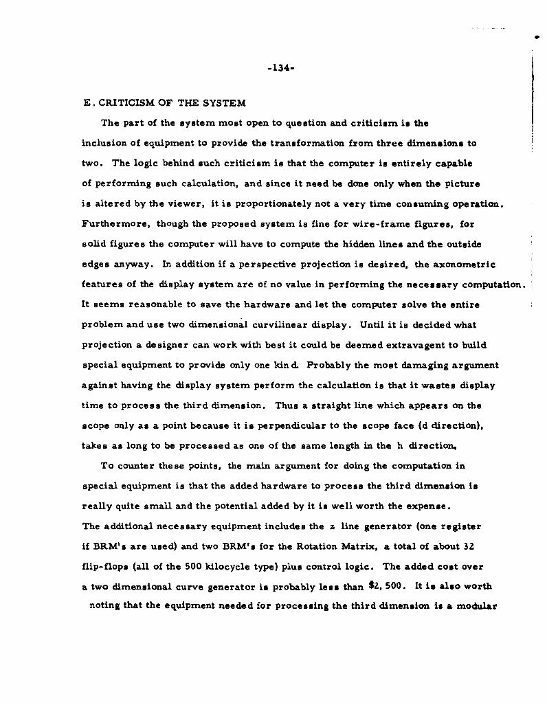
C
-134-
E. CRITICISM OF THE SYSTEM
The part of the system most open to question and criticism is the
inclusion of equipment to provide the transformation from three dimensions to
two. The logic behind such criticism is that the computer is entirely capable
of performing such calculation, and since it need be done only when the picture
is altered by the viewer, it is proportionately not a very time consuming operation.
Furthermore, though the proposed system is fine for wire-frame figures, for
solid figures the computer will have to compute the hidden lines and the outside
edges anyway. In addition if a perspective projection is desired, the axonometric
features of the display system are of no value in performing the necessary computation.
It seems reasonable to save the hardware and let the computer solve the entire
problem and use two dimensional curvilinear display. Until it is decided what
projection a designer can work with best it could be deemed extravagent to build
special equipment to provide only one kin d. Probably the most damaging argument
against having the display system perform the calculation is that it wastes display
time to process the third dimension. Thus a straight line which appears on the
scope only as a point because it is perpendicular to the scope face (d direction),
takes as long to be processed as one of the same length in the h direction.
To counter these points, the main argument for doing the computation in
special equipment is that the added hardware to process the third dimension is
really quite small and the potential added by it is well worth the expense.
The additional necessary equipment includes the z line generator (one register
if BRM's are used) and two BRM's for the Rotation Matrix, a total of about 32
flip-flops (all of the 500 kilocycle type) plus control logic. The added cost over
a two dimensional curve generator is probably less than $2, 500. It is also worth
noting that the equipment needed for processing the third dimension is a modular
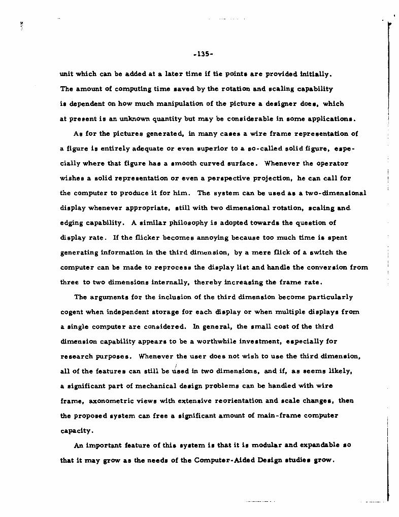
-135-
unit which can be added at a later time if tie points are provided initially.
The amount of computing time saved by the rotation and scaling capability
is dependent on how much manipulation of the picture a designer does, which
at present is an unknown quantity but may be considerable in some applications.
As for the pictures generated, in many cases a wire frame representation of
a figure is entirely adequate or even superior to a so-called solid figure, espe-
cially where that figure has a smooth curved surface. Whenever the operator
wishes a solid representation or even a perspective projection, he can call for
the computer to produce it for him. The system can be used as a two-dimensional
display whenever appropriate, still with two dimensional rotation, scaling and.
edging capability. A similar philosophy is adopted towards the question of
display rate. If the flicker becomes annoying because too much time is spent
generating information in the third dimension, by a mere flick of a switch the
computer can be made to reprocess the display list and handle the conversion from
three to two dimensions internally, thereby increasing the frame rate.
The arguments for the inclusion of the third dimension become particularly
cogent when independent storage for each display or when multiple displays from
a single computer are considered. In general, the small cost of the third
dimension capability appears to be a worthwhile investment, especially for
research purposes. Whenever the user does not wish to use the third dimension,
all of the features can still be ised in two dimensions, and if, as seems likely,
a significant part of mechanical design problems can be handled with wire
frame, axonometric views with extensive reorientation and scale changes, then
the proposed system can free a significant amount of main-frame computer
capacity.
An important feature of this system is that it is modular and expandable so
that it may grow as the needs of the Computer-Aided Design studies grow.

-136-
Furthermore it is adaptable as applications arise for the systems in other
fields of endeavor. The potential of on-line man-machine interaction is tremendous
and is largely unexplored. The display scope no doubt will be a vital link between
the human and the computer in any such studies. By emphasizing its modularity, the
display system will be a powerful research instrument in the entire man-machine
communication problem as well as the medium for graphical input output for
the Computer-Aided Design project.

APPENDIX A
PROGRAM DESCRIPTION
The simulation program written to study the characteristics of the
display system was done on the PDP-l, a small general purpose computer
at M.I.T. which is manufactured by the Digital Equipment Corporation.
This machine was chosen because of its availability and its excellent
display scope. The PDP-l is an 18 bit parallel computer with a 4, 096 word
core memory. The machine's principal input means is by paper type,
although an on-line typewriter is also available. The machine also
possesses 6 Sense Switches and 18 switches of a Test Word which can be
sensed by the computer at any time in the program. These allow easy
switching between operating modes so that various configurations of the
system could be compared.
The program operates on a display list which is similar to the
list described in Chapter 11. This list starts in register 30008 of core
memory for all displays. Thus it is easy to change the picture entirely
by reading in a new tape which reloads the data starting at 3000 thereby
replacing the contents of the display list.
The first three words of the file comprise the heading and specify
1) the number of lines in the list 2) the hostarting point 3) the v0 starting
point. The rest of the display list is a series of descriptors to call out
lines to be displayed. Each descriptor requires four computer words;
1) a control word to specify the type of line and its length Z) x BXM
starting condition 3) y BRM starting condition and 4) z BRM starting
-137-

-138-
condition. If the line to be drawn is a curved line, the z BRM is not
used (all curves are generated in the x, y plane), and the fourth word of
the vector descriptor specifies the length of the BRM to be used to
generate the curve. There is one configuration of the control word which
causes the nine terms of the matrix to be matrix multiplied by the 9 data
words which follow the special control word. This allows rotation of the
curves to any orientation desired.
Control is provided by six sense switches. The first three are
for rotation about the three scope axis h, v and d. The fourth switch
resets the rotation matrix to the unit matrix. The two other sense switches
provide magnification by factors of two and four. This magnification is
done by spacing all the points of the display further apart, so that details
of the points constituting a line may be scrutinized.
Additional control is provided by 18 switches of the Test Word input.
Two of these switches permit further control over the size of the picture
by causing the program to multiply all values of the rotation matrix by
a number slightly less than one or by a number slightly more than one.
Four more Test Word switches are used to cause horizontal and vertical
translation of the starting point of the picture. Other Test Word switches
are used to switch in and out of various modes of operation. These include:
1) a switch to select BRM or DDA as the basic unit of
the line generator
2) a switch to call in the perspective projection computation
3) a switch to bring in the smoothing logic (one versionhas the smoothing logic based on the three stage shiftregister, another uses the look-ahead logic)

-139-
4) a switch to call in a sine-cosine routine to providea true circle for comparison purposes
5) a switch to select a mode which generates a figurefour times as accurately by the techniques describedin Chapter III
6) a switch to change the sequence in which the BRM'sor DDA's are processed, in order to control whetherthe stable equations or the unstable circle equationsare generated. These equations are discussed inChapter II
7) a switch to apply a one stage backlash unit at the inputto the h and v registers
8) a switch to select the logic required to test the attemptsat averaging the round off errors
Figures A. 1 through A.4 are flow diagrams of the basic program. Only
Test Word switches 1, 4 and 6 are included in this version. In summary the
program consists of three main loops inside each other. One complete pass
through the outer loop (loop 1) generates the entire picture. A pass through the
next inner loop (loop 2) produces one complete line. A pass through the inner-
most loop (loop 3) represents all the processing done on a single clock pulse.
Starting with the inner loop, the program generates a single clock and
looks for any output from the line generating unit. If none occurs it checks
for'bnd of the line'and then recycles. When an output occurs for x, y, or z
this pulse is carried through the rotation matrix, the new point is plotted
if applicable, and the x or y data register is changed if a curved line is
being generated-- all before the next clock cycle is entered.
When a single line is completed, loop 2 is cycled. A test is performed
to see if the line just completed was the last line in the list. If so the outer
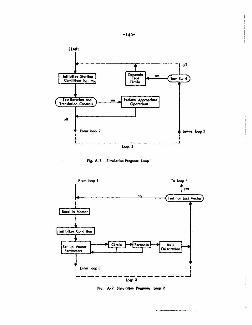
-140-
START
Test Rotot on and on Perform Appropriate
Translation Controls Oeain
Off
Enter oop 2Leave loop 2
Loop 2
*Fig. A-1 Simulation Program: Loop 1
From loop 1 To loop I
94 noTest for Last Vector
Parameters r = to o
IEnter loop 3
aLoop-3
Fig. A-2 Simulation Program: Loop 2
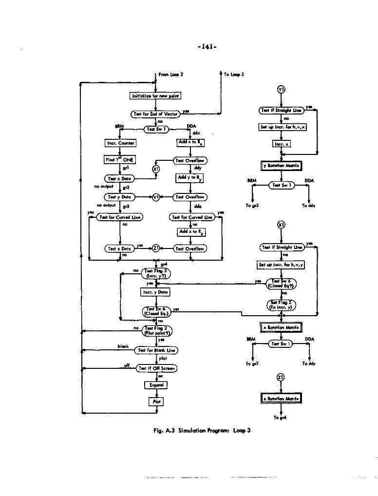
From oop 2To Loop 2
vi
Tat fr End VetorTest If Straigh Un. e
no
TestSW IddxSet up Incr. for h,v,x
Incr Couter to xIncr. x
94 xiy Rotaton Matrix
Test~~~es yw 1etI Ts vrlw
"Fig A.3~u Simlaio Proram Lop q3 T

-142-
Ner Rotation Matrix
Increment "e"Coune
Tetr to Outp
Nom P :M
output Se .1
04 Increment v
JP
Return to he"
Fig. A-4 Simulation Program: Rotation Matrix
-143-
loop is cycled. If not, the next vector on the display file is read in
and the necessary initial conditions are set up. Then the inner loop is
re-entered.
The outer loop initializes the necessary registers for a fresh start,
then tests to see if any alterations to the parameters of the system
should be made as called for by the operat or with the rotation switches
or the translation switches.
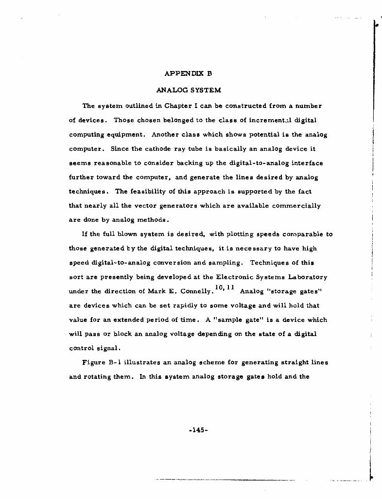
APPENDIX B
ANALOG SYSTEM
The system outlined in Chapter I can be constructed from a number
of devices. Those chosen belonged to the class of incremental digital
computing equipment. Another class which shows potential is the analog
computer. Since the cathode ray tube is basically an analog device it
seems reasonable to consider backing up the digital-to-analog interface
further toward the computer, and generate the lines desired by analog
techniques. The feasibility of this approach is supported by the fact
that nearly all the vector generators which are available commercially
are done by analog methods.
If the full blown system is desired, with plotting speeds comparable to
those generated by the digital techniques, it is necessary to have high
speed digital-to-analog conversion and sampling. Techniques of this
sort are presently being developed at the Electronic Systems Laboratory
under the direction of Mark E. Connelly. 10,11 Analog "storage gates"
are devices which can be set rapidly to some voltage and will hold that
value for an extended period of time. A "sample gate" is a device which
will pass or block an analog voltage depending on the state of a digital
control signal.
Figure B-1 illustrates an analog scheme for generating straight lines
and rotating them. In this system analog storage gates hold and the
-145-

-146-
0
-~ 0
2 4A IA
U4.
34N
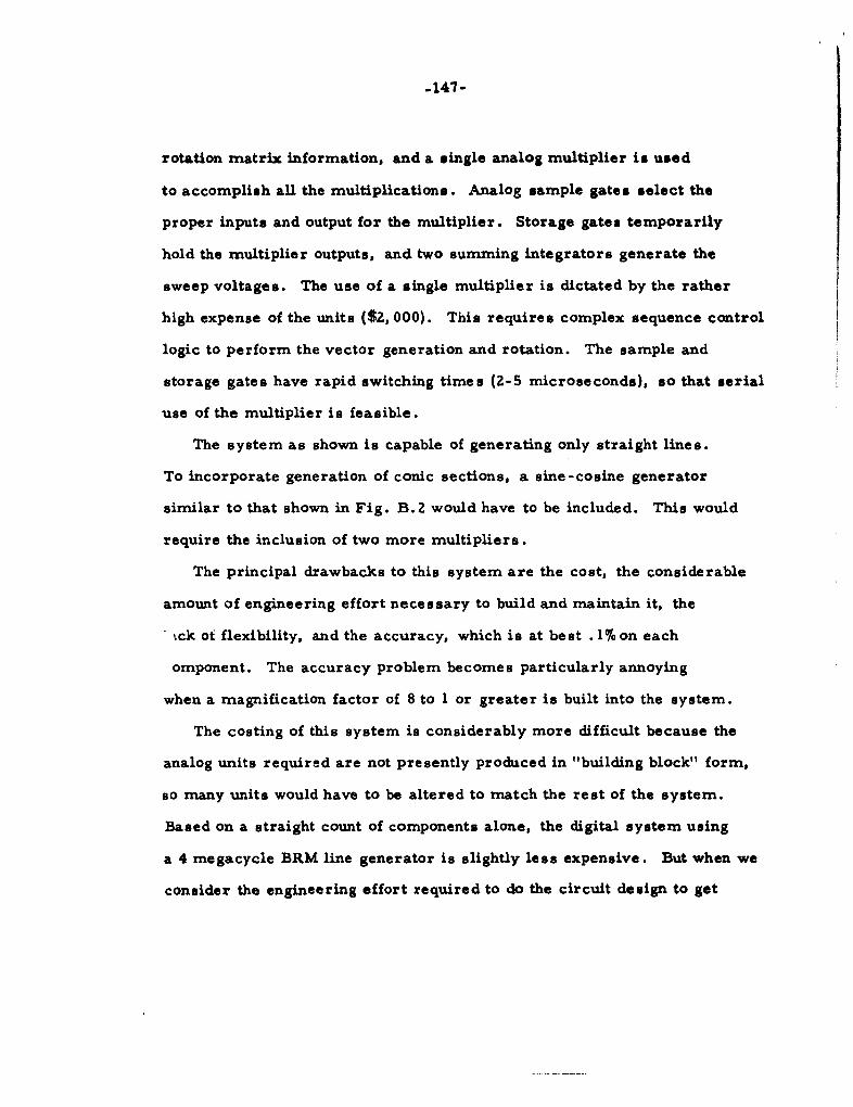
-147-
rotation matrix information, and a single analog multiplier is used
to accomplish all the multiplications. Analog sample gates select the
proper inputs and output for the multiplier. Storage gates temporarily
hold the multiplier outputs, and two summing integrators generate the
sweep voltages. The use of a single multiplier is dictated by the rather
high expense of the units ($2, 000). This requires complex sequence control
logic to perform the vector generation and rotation. The sample and
storage gates have rapid switching times (2-5 microseconds), so that serial
use of the multiplier is feasible.
The system as shown is capable of generating only straight lines.
To incorporate generation of conic sections, a sine-cosine generator
similar to that shown in Fig. B.2 would have to be included. This would
require the inclusion of two more multipliers.
The principal drawbacks to this system are the cost, the considerable
amount of engineering effort necessary to build and maintain it, the
.ck of flexibility, and the accuracy, which is at best . 1% on each
omponent. The accuracy problem becomes particularly annoying
when a magnification factor of 8 to I or greater is built into the system.
The costing of this system is considerably more difficult because the
analog units required are not presently produced in "building block" form,
so many units would have to be altered to match the rest of the system.
Based on a straight count of components alone, the digital system using
a 4 megacycle BRM line generator is slightly less expensive. But when we
consider the engineering effort required to do the circuit design to get
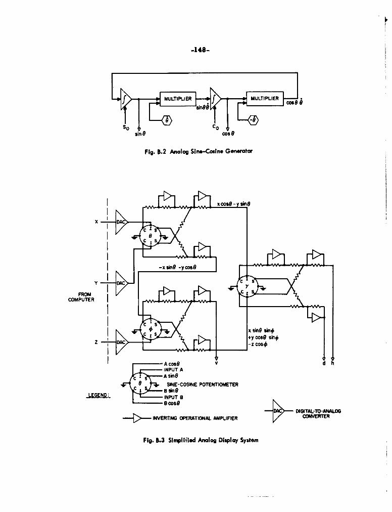
-148-
fMULTIPLIER *fMULTIPLIER cssin~h
SO COsin 9 8 ose
Fig. B.2 Analog Sine-Cosine Generator
xcs V oO-Ysn
A s n
COMNPUTER
DcDGTL-OAAO
-i>.---~~~~~ INETIN OPRAINAnAPIFE
Fig B.3 Simlie Anloiislany#e

-149-
the high speed performance, to "mate" the units to the system and to
design the large amount of control logic needed, we see that the analog
system will be more costly and will require more development time.
Furthermore analog elements tend to require more maintenance after the
system has been built.
The analog system also lacks the flexibility that the digital system
offers. As a research tool, the display system should be made so that it
is easy to change to try new techniques. For instance the accuracy
of the rotation matrix of the BRM system can be improved at any time
by adding more bits to the appropriate BRM's. For the analog system,
precision is fixed. Also such techniques as "automatic pen tracking"
can be more easily incorporated into a digital system.
The accuracy of the analog system is hard to evaluate since the system
can not be simulated as the digital system was. The inherent drift
problem in analog devices is emphasized because of the high gains
required to meet the switching times which are demanded of the system.
However this is probably not as critical as might be expected, since
long time stability is not so critical in a visual display being regenerated
every thirtieth of a second. However accuracy is linked directly to the
picture size as well as plotting speed. Thus if magnification control
of 8 to I is incorporated and each component is accurate to . l¶/ on
the expanded scale errors of 20% are possible. This combined with a
slow drift of the picture would be most annoying. In the digital system,
stability is assured and accuracy is related only to plotting speed.

-150-
A second analog approach was investigated which considerably
reduces the expense, but doesn't help the accuracy difficulty, and also
lacks flexibility. This uses sine-cosine potentiometers connected as
shown in Fig. B. 3 to provide the rotational feature.
This configuration generates the following matrix equation:
-cos 6 cos Y sin • cos Y cos sin Y x h
-sinesin 40 sin y -cos 8 sin 4 sin y
cos ý sin e cos cose sin Y V
-cos 9 sin y sine sin y-sin 0 sin 0 cos Y -cos sin 40cosY cos cos Y z d
which is the equation for rotation about the three axis taken in the order
, *, y; where e is the angle about the z axis, * is the angle about the x
axis and y is the angle about the y axis.
Under this scheme the viewer has control of the orientation of the
picture by three knobs controlling the three sine-cosine pots. A similar
arrangement has been used before12 quite satisfactorily to give 3 dimensional
display with just 2 knob control and for rotation of a single straight line
figure it is entirely satisfactory and considerably cheaper than other
schemes. Unfortunately, however, this system does not possess the
versatility required for the general display problem, because the computer
no longer has any control over the picture orientation. This is particularly
bad where special functions are to be generated. By providing a computer

-151-
control over rotation, a single function generator can be used to
provide the function trace, and the rotation matrix can transform the
figure to any desired orientation. Without this facility the function
generator must be capable of producing curves at any arbitrary
orientation, which requires considerably more computational power.
I
BIBLIOGRAPHY
1. Investigations in Computer-Aided Design, Interim Report 8436-IR-1,Electronic Systems Laboratory, Massachusetts Institute of Technology,Cambridge 39, Massachusetts, January, 1961.
2. Sutherland, Ivan E., Sketchpad, A Man-Machine Graphical CommunicationSystem, ScD. Thesis, Department of Electrical Engineering, MassachusettsInstitute of Technology, Cambridge 39, Massachusetts, January, 1963.
3. Randa, Glenn C., Design of a Remote Display Console, M.S. Thesis,Department of Electrical E-.gineering, Massachusetts Instituteof Technology, February, 1962. Also published as Report ESL-R- 132,M.I.T. Project DSR 8753, Electronic Systems Laboratory, MassachusettsInstitute of Technology, Cambridge 39, Massachusetts, February, 1962.
4. Randa, Glenn C. and Grondstra, J., Design for a Manual InterventionConsole , Internal Memorandum No. 8753-M-55, Electronic Systemsabioratory, Massachusetts Institute of Technology, Cambridge 39,Massachusetts, March, 1962.
5. Haring, Donald R., Analysis and Simulation of Incremental ComputationsPerformed by Binary Rate Multipliers, Report 7849-R-10, ElectronicSystems Laborator:y,"-ssachusetts Institute of Technology, Cambridge 39,
Massachusetts, April 1960.
6. Hills, Frank B., A Study of Incremental Computation by DifferenceEquations, M.S. Thesis, Department of Electrical Engineering, M.I.T.May, 1958. Also published as Report 7849-R-1, Electronic SystemsLaboratory, Massachusetts Institute of Technology, Cambridge 39,Massachusetts, May, 1958.
7. Lundh, Y., "Digital Techniques for Small Computations", The Jorna.lof the British IRE Vol. 19, No. 1, January, 1959, pp. 37-44.
8. Digital Modules, Digital Equipment Corporation, Maynard, Massachusetts.
9. Julesz, B. and Miller, Joan E., "Automatic Stereoscopic Presentationof Functions of Two Variables", Bell Systems Technical Journal, Vol. XLI,March, 1962.
-153-
-154-
BIBLIOGRAPHY (continued)
10. Connelly, Mark. E., Analog-Digital Computers for Real-timeSimulation, Report ESL-FR-I 10, M.I. T. Project DSR 8215,Mlectronic Systems Laboratory, Massachusetts Institute of Technology,Cambridge 39, Massachusetts, June, 1961.
11. Binsack, Joseph H., A Pulsed Analog and Digital Computer forFunction Generation, M.S. Thesis, Department of Electrical Engineering,Massachusetts Institute of Technology, June 1960. Also published asReport No. 8494-R-2, Electronic Systems Laboratory, MassachusettsInstitute of Technology, Cambridge 39, Massachusetts, October, 1960.
12. Mackay, D.M., "High Speed Electronic Analog Computing Techniques",Proceedings of the Institute of Electrical Engineers, Vol. 102, Part B,(1955) pp. 609-620.
13. Hildebrand, F.B., Methods of Applied Mathematics, Prentice-Hall,Inc., New York, 1952.
INITIAL DISTIBIIUTION LIST FORCINTRACT AF-33(dOO)-4289
DII 8733 2/63
Aeronca Manuflacturing Corporation. AVCO CosrpootienEngineering ULibary LcmigDvso
Engieerng epotamerkAttn Dr. Hans Klein
GOVERNMENT AND MILITARY Engineng , OhoChe, Go Tatbsine
Stratford, Connecticut
Air Force Meom Prod. F ..ipsasent Aronutronic Btatlefe Mesmerisl lestlhut
Atn r oetW hlisDivision Ford Motor Coompanry 50 Kng NA.en eReitributMr. Group Ubray At:M.CalsE a
PentagD23 onlo Ford Road eatU..
AMC Bollsstic Missiles Center Aerospace Industrioo Ausacition Beech Aircraft Comepany
Attn: UIFE (Mr. F. Becker) Attn. Ubrawy Attn. Lt H. OwenAir Force Unsit Poet Office 1725 DeSoles Street, NW Mgr. Manufacturing Engineering
Amny material Commmand Board Aerospace Industries Association Bell Atrarft CorporationAttn, Col. D. Mac~etet Technical Service Ubmay Attn. .17.C PAIiliiiinAkeodion Proving Ground Attn. J.A. Maurice k -oge Production EngineeringMorylord 7660 Ieveriy Boneyard Internal Zwon C-93
Lot Angeies, Caiifornia Buffalo 5, Ne" York
ASTIA (10) Airbsorne instruesents Lobsatry Bendix CoreorotionArilngton Hail Station Attn, Miss Nancy peannier Alttn CentraliLUbraryAriington 12, Virginia Wait Whitman Road Deoartinont 75
Melville, LI., HNow York. an 1139Kansas City 41, Miesouri
Co-seander Allison Division GMC The Bendlix CorpoartionAeronautical Systease Division Afttn Engineering Ubroy, Plant 8 Industrial Controis SectionAttn: Mr. W.M. Webster ASECTP P.O. BNo 894 Atitn Technical LibraryWrIght-Pottetion Air Force Bose, indlonIpoIts 6, indiana 2182 WyasengOhio (2 and letter) Dettoit 37, Michigan
Con'monde Aiumlwnm Company of Amserica The Bni..l CorporationU.S.N.O.T.S. Attn. D.i. Alkire, Proect Engineer Attn.s Mr. GS. KnsopfPasadena Annex. 2210 Harvard Avenue 2182 WyowtingAttn. J.H. Jonnirson Cleveland 5, Ohio Detroit 37, MIchigain3202 E. Foothill BoulevardPasadena, California
Commeanding Officer Anerican Machine and Foundiry The Bendix CorporationOrdnance Materials Em. Office Eieeorch and Develicpment Division Altn. Reports LibraryWatertow, Arsenal Attn. Ubrory Research Laboraroria Divisionjttn. N.L Reed, Amst. Director 6819 Hope Street Southfield, MichiganWoteft-w 72, Maueohueett. Staniord, Conneacticut
Director A.O. S~rth Corporation Ma ivitionNaval Eesearch Laoraotoriee Attn. Technical Uibrary Ditn Tec nicl.ssnAttn. Code 2021 P.O. Box 584in ehnclU.aWashington 25, D.C. Milwaukee 1, Wisconsin Mro, Penrayivenila
U.S. Atormic Energy Coannission Anon,." Research Foundation The Boesing ComenTechnical Infonnotion Service Attn. Dr. S. Hod MASO-WIchia racP.O. Boo 62 Senior Reeearch Engineer AttSn: s 710Ury1Oak Ridge, Ternseasee l0OWest 35th Street 311SuhOie
Chicago 16, Illinois Wichita, Kaorms
Arthur D. Atte Icroatdlon. NOE. Laughl nAttn. Miss Dorothy E. Hart fn . LuhiLibtary (Et. to David N. Smith) O~ris. 2-3 930 Nti 45-33Acorn ParkP..2" 011
INDUSTRIAL AND UNIVERSITY Cambrdge 40, Massachusetts Seattie 24, Washsington
Aenalet-Generol Corporation Astonstics TheBoigo anAttn: Myra Gronter, Ubrarla Division of North American Aviation, Inc. Antn. G.M Pai . . 2-3010iWO0 W. Hollyvale 9i50 . imsperfal Highway, 3041-13, Bldgt. 60 Numesercal Coetrol alpreseietiAzuwe, Caiorila Attn ILL Pborsk, Technical Ubrat P.O. Ban 3707 MS. 12-61
Dowsney, California Seattie 24, Washington
Aerojet-Generol Corporation AVCO Corpoatin The boeing CompanyAtit, Technical Ubray 24i20105A iLycossing otvie Attn. 1J. CeriberifP.O. Box 1947 Atn.e H. Meehi Catli.2.5-321sac mmwnt 9, California immpeltse~nt Manufecturing Engineering l1~ed M bIS 4
Stvaford Ccrsectcs~tSeatle 34. Washington

DWI Swassok sad Norawum loPmd Caro~l"A101 CaatOMMGawa Mi.. SaiNWe LAN
Cerda25 eesatl 'I Mile wal Menod Nsals
Swe~~rpatnDivision tiroredo Olxvhlos W a. N L~w Ide
Me.:U1.w Fend D. LOCI Wisonswin
"440 Slaekls. Villa m
IeadNe California Ln OA aiona
~-'hefltataofDouglas Alroraft Cosepanry, Incorporte GoTadftavMesNK.Shappall, ' ise M19 swPlnnn
Systmenew en pnd -dia Sclefte Missiles ado Space Division Mtnn Librarian
Scholedy ew&k Sont M~ie., California 1210 Massillon Real
Pittsburgh 13, Pennsylvania Mauim 15, Ohio.
Corneille Institute oF Technology AIircaft.O Consony Inopracl Orunown Alrc=6ft k¶Cwlriion
nlwJ~ LlroyDo A2-260 :toopgL.I.,Now York
Pittburgh 13, Pavoaylvemle .0 Monica, Callifona
CEII Incorpara Eb-Cal - orpraIon Grumeman Alrarelt Engineerin CorporatlioAoLL.Too Afl~u: John F. GwenMe. 0. D. Fogell
621: Fosolo Avrns Numnsr-Troll Sage A~jtoineec COrcPflln GrouAp
Connncticut P.O. Box 366 Flant SDetroit 32, AMcicgan Se0paL I., Naw York
CN arwOpica Comapny, Incorporateci Gruman A1Mrarft Engineering Corporation
10 efrw-wsHsny40 *Boleard Mate" T'=n I~rng, Fant 3Arlhqgto: 2, Virghini Naw York 70, New York Sa0pgNwYr
Ceomm Alrraeft C~ompan Fornaowl Electric IncorpoHilled Al11 Nrorft CorperstlenSSU les Faunae Mm:n t. MII Dewlet Ilnuolg sad! IAeark LibrayMm:n EnagnawlIng Library Plawlelw, L.I., New York 19"70 Wlow teodWichita. Kano Pale Mlto, California
Chance Voughte Library Fr oo ~M ~ ~ r lge
Unit 1-4101 Men: PIG Cadra, .. 7,C1 ts`g. Ftatiolt.-C~gqblrd, Schuyler, Sch1:Wl Ir.De.3 TraaChwasl DIvIsdo Menn. Plt ULibrry, lId6
P.O. ha Sw7360 PIr.esutosla Tucson, ArizeonaDalias 22, Teans Live"i, Michigan
CinInnat "I mlling Mechine Comepany Franklin lInstitute Huoghes Tool ComapnyMe.:'Aý Ml.tnAn a Motion jet ewon Mset William W. Lesepkin
EnieerngLbrr Technical I~ Ukowya V.P. We~. Alrcraft Dvso
Odakly Cincimad 9, Ohio 20th gad Parwo Florence Avenae and Teala SemiWhldep~ 3, Peneyvana Culver City, Ca~llfoes
CIncInnatIl Milling a Achine CeApOry General Dynagilot-Meronautlis Ilyda-MII CorapanyAmn Dr. Iena Morales Digital Cosspothai Laboritoy Mtn: Wa. Hwry lEmch V.P.4701 Markurg Avenue Assis K. W. Isekow 17017 Cleverfied Seolavrd
Mllaall 9ZOi Mi oer 1101 -0 Sente Monoda, CeliforniaClncmetP, 61.P.O. han 1128
Son Diego 12, Colifornia
Claeladm PeouwAilc Tool Company Gemneal M ancs-.Port Wort: Division IsmMe.: boecigLbrr.t" J. McWhorter Mein: L 0a4
3 E.7tStetDept. 6, han 0I11 Meek ada Applications Dopt.
Cloelaalad5, Ohio Awasytsas ,#eaeC ationoI Laboratory 1271 Avenue of AssarloesP.O. san 740 New York 20, Nen, YorkFort Worth, Tao.
Concord contral Incorporaed Gomoel Electric Compansy IBM Lieor OfficeAmn: Wa. .. 0. McDoneoh, Free. Mona -.Achorwed Morsocturnglng. Rome 26-447
Soen35, WAWocýhoel UID-Mesvsfacturlr Op. Mall Cede 1.122 77 Massachusetts AvwwuSulkdlng 700, Iwnel Plat Ceebkrld 39, MaeschsacletsClMncnnie 15, Ohio
ContlmInta Aviation wad Engineering Corp. General Electric Ceeorsy 1WM Dae fto1% hng DivisionAtnMTcnia ibay sW. W.~ec Spn , WagAt~ . P. 1. Cnqipeeoor
127n0 TeK~a Liktveu I cn bhy P.O. han 4014imot15 Wordnow 7 eigo Avenue SeverWbue~6leny Hills, California
Nee York, 22, New, York
Gona Electric Ceapasy lak Corporation
=ee-t Me. In oto CPA 0. Norane II. Taylor, V.P.Vw= .I% ore conrol Sales) 10 Maguire Read
Way a" ILexnrgton 72, Mocoechsaatt
DiIsionlof General Dyneetecs Corporation Men.:Yosw"nMtH .Hod e.0Me.: ft. M.D. W~l~ao Technicael Lkibray SakfoVrChlef of pledMfg. Son ad F eot Den. 3415 Weas Fierce SteetPacific iirepMilwasben is, WisconsinSon Dtege 2, Ceilffrnle

se, . Marorhl Eectric Corporetion North Aeserican Aviation, Incorporated SAttn Aseociaese bo.86
eres
Atnt. J&., Olson Atnne Technical Libray Ats TwadLirr
ChieE Engineer Iinesotmlenl Airiportil Sm
P.O. gso 11275 StatiosnA Lo Angeles 9, CaiifoireoNo ,M oi
Paio Alto, California
ee,,edTrecker vim Noorth Ameerican. Aviation, Incorperte ania
7Atn a~ ~=r~ 1c*L0:moy Atne; Whitman C. Walter 0DA07-M3 LUverro
11000 Theoedore Tracker Way IntenatonelAirsrt ttn
Mlleseukee 14, Wisconsin Los Mgeolas 9, California P.O. Boxe
K"MnfcuigCmayNorth Americani A~ioaton, Incroae The Semrvice Owaso. Corporation
EP auatrn g CoepLany Attone 0. Dole Smith, DA187= esc Iaeleo Avenuey
LOC.s A, n-menueAipr 35Mdsn voo
Rowelond, Ne" Jersey Los Angeoles 9, California New York 22, Now York
LaihCmayNorth Amemrican Aviation Incorporated Sikorsky Aircraft Division
Lodi Msh lupcl Co brany Artone t*. Roeeart G. Heclcwohon UiMted Aircraft Corporotieon
5481 S. Packard Avew, Numerical Sciesncxes Group 282-072 Attn.s LI~
Cudahy, Wisconsin internotionwl Airport North MantreeltLos Angeles 9, Coilifornia Strotford, Connecticut
Lociheed Aircroft Coonponmy North. Americane Aviation, Incorporatee4 Soler Aircroft Coenpany
AteDr ..FrihAttn, Theeicl 11.Fees 01tio Center Attn.t J.A
O ro. 7901 Fuldngi13t30 E. "Fifth'Avenue Mfg. lect vItioneSunnyval1, Culidoriag1 Coiuabus 16, Ohio Son Diego 12, California
Lockheed-California Conpony NortrwopCorporation Sperry G ComopmeyMin Cetra Lirar Noeal Diisin tone 1nginer Lifrery
ADn oto irr Altne Technicol infor maion, 3924441 Mail Station IA35'e%..72-25, muilding 63 11 .kdwyGreet Neck, Noew York
LokoslArrf oprtmNoreronics-Systeee Support Sperry Rand Univoce
Lockhed oArcot Corporotione Gordon Wilcox, Librarian Nmemericall Conro
Attn R MerthosEo 500 L Orongethore Avenues Attne Gastoneo Chingeri
. yodwa Atnaholel, Colifornia 2520 Went Sixth Ptreet
Bshebar, Colifornia Los Angeselems 57, Californio
Lockhesed Aircraft Corporation Onseud Machine Works, Incorporoted Attnho EngineerIngsLitutyScienceo-Teechnology Informastion Canter Attn.t h~r. Eerie Ptrkcnnlr tmEoomrn irr
Dempt. 72-34, Zone2 V.P. Director of Engineering C41010 PrkiMariatta, Georgia 2 7700 North Lehigh Avenue Clfri
Mconnell Aircroft Corporation PhIlco Corporotion Stenord' RQseech Institutes
McDonnell Automation Center C end I Divisio Altne fMr. P.D. Tilton
Dert 73 Attne Moom C. Ferguson, Libraran Indusetrial Reseemrch Enginee
P.O. bon 516 4700 Wimsshickosn Avenue 62 Mink"o Stree
St. Louis 66, Missssi Philadelphia 44, Pnerseylvonlo SouthP--'ee California
Mclonnell Aircroft Cooperation Republic Aviaion Corport'tion St, Isch CR.oporokes
Ann Enegineering Library Atn 1oa Mttn: V.CEr-e GlorestgEgiern
P.O. Nt 1 6 Fermi,..4
40i, L.t., Noew York 635 South Main Street
St. Louis 66, Miuaotr Southe Band 27, Indiana
The Marquardt Crpoerotlone lobeort A. Key" Assocksteion S- ds'en Mochinoe Toni
Mattn W.E. Otto, FomnMaronoer Anni Ak. RosA. Ketes Dircte Gods Enieering
Sam 670 821 Franklin Avenuecm f einwn
Ogden, Utok Goordon City, L.i., Nen, York Seelvideore, lilinelto
The Merquerdt Corporotion Rocketdyrm $yet-a Dervoepopnssnt Corporation
Attn: Engineemring Likrary A Division of North Atnericomn Aviation, inc. Technmicel Librery Semrvices
16553 Sotico street Atn. Library, Deortment 586-306 Er. to A. Roeener, C. Keliage
Von Nuys, Colifornia 6633 Comeg Avenue 2500 Coloredo AvernueCaogmo Perk, California $Soantme Mnce, Celifornie
The Morquerdt Corporation Eocksotdynee Teesco Electronics
Atetn E. C. Krueeka A Division of North Americen Aviation, Inc. Afttn Ubekery DPto. 403
Mail Zeom 21-24 Solid Rocket Division P.O. See61 It
1655 Saticoy Stree Altn. Liberar Dalles 22, Tanae
Ven Nuys, ifanlo McGroegor, Teem
Th atnCossipory() luke Corporetion Theempoeo Reade Woeoldiids.
Aeseru Librr7y,A-t52 Attn D.LS. McCoy Amt. Mission
P.O. WaK19 u to L.L isign P.O. S=en 6M73lboek vom
Denever 1, Coloredks Chule Vioew, Celifornia Commoe Perk, CeolifesnI-
National Machines Toni Md4. Ason Ryan Astonautical Company Ro We hg
Athos Thesne L Licyely Most Pfeslest L.Cark Come" Sydo
2129 Wisconsin Avenu 2I01 Isfuker Drive tuigAneJ .Okf'hg. fIS
weslngon , DC.San Dingo 12, Celifornia Michigest city, iwdlette

ThomsonEm Wol~ge Iom~iedAAOITIOM
23W5 Eualid Avenu
us" cr" Ncloorr, rridon Laboratories, lon..MMt. .LL w GehLno Mt. . Dan Read
Alin J. vdJr.1324 W. WUecwmn AvenueP.O. e Is milweuldw 3, WisconsiOmk Ridge, Tame...s
Wiedwc Asisomworpoella Um Industries Assoc of Anarico, Inc.Ea~wh Lboroorle Urory~ M. SD. Daniels
!ota Is itare 8, Conn~ecticut Director of Te~clgcl Sw~ay!1725 DeSela Street, N.W.Wahldnoten 6, D.C.
Uniled AircredI Corporellon Thompson Rom. WooldridgeResearch LowwwtwI4 LW. DivisionAMs. C. Roblskmn I "oes aln Iyat~e. DeparteentEmt Nietff , Conectlcut Mtr., Jid.. Me"w R. Pintev
S43 Fodllhook Avernuecamps P"n, California
Uniled Stole Rubber C o.e.opeIseniCopoatoResearch sed Do... Dept., Lihewy Syte ,, " p oprto
W"., Now Jensey Tune wal Avarwy
Lacingien, Massahusetts
Wilvoc Divide. lessngton Rand Is mMt.. tid.. WA.Larc Mtt., Jeoe. So-wee
Now York 10, Now York
Walvac, Divisio Sperry Rand Corporation Director .f Siehloodrel Sciences and Commommd and ControlMltnt Isr. LW. ba~ Office o1 Secetroly of Defense351 Park Avenue Sout AA.P.A., PassegoNew York 10, Now Yark Waoglotn 25, D.C.
University of Celifernia Mr. Prawd, Elogl, Jr.n , meo 0d lselno The Comrputation LabommonyMltn, Dr. Amie=.Reeensten 01tofilood Wtvemety405 Willord Avenue 33OddSreLos Anipeles 24, Cellferni Ca=.de enouet
The Wsomerml ad R Ae SuwbCenter Professor L. J. LeoneMt.,t Mr. S.P. Wknchel, Etectricol Emon91neer;eDepeteaVmeDhreco of a eoc, and Develp t nierit of Washlogen
Cievotaed 39, Ohmo
The Wasn e nd Say Cepempny Office of Novel ReseachMit. Tee-eth1o Libary inormIon System.Ioc5701 Cuv.eml AVe"" Mnt. Mr. 0oel i K. Pollocit
ablkd1,oe, Code 437Wabogtovn 25, D.C.
-ekhm Electric Cmp01
Stesen Dl Aw*ilay
TWheON Movreal CoroationP.O. me 103
Stee3, Mw;Armd
;oastion =n CeseftyTeciegoloi inea ONen Centerwere@"i 1, lemmedenen.

zn z 0ýW
w u w U
.: A :, - -V~r 0 .0 UL 0
-k0 .,-, U K & .- I.. s oI , 1 0
aL. 'oi ~
wo- e-w 0 'u a<tt 01 oE 0 z0 ZS 0 -
A 0 rz z1
I. ONI - Ul .( -0 v v'-. V IL U
!,.1 04 0 0n 1
. 1 !; ~ - -o0
AE ou a ua A 3 1 1 V 1
o < 1 wn- .0 *-04
U.u-:'~, U