Uncertainty,sensitivityandrejectionin ! …cees.stanford.edu/docs/Caers-slides.pdf ·...
37
Jef Caers Stanford University, USA Uncertainty, sensitivity and rejection in predictive reservoir modeling
Transcript of Uncertainty,sensitivityandrejectionin ! …cees.stanford.edu/docs/Caers-slides.pdf ·...
Jef Caers
Stanford University, USA
Uncertainty, sensitivity and rejection in predictive reservoir modeling

Quantitative modeling of geological heterogeneity Modeling uncertainty in the context of decision making Building 3D/4D models accounting for scale and accuracy of geological, geophysical and reservoir engineering data
Stanford Center for Reservoir Forecasting
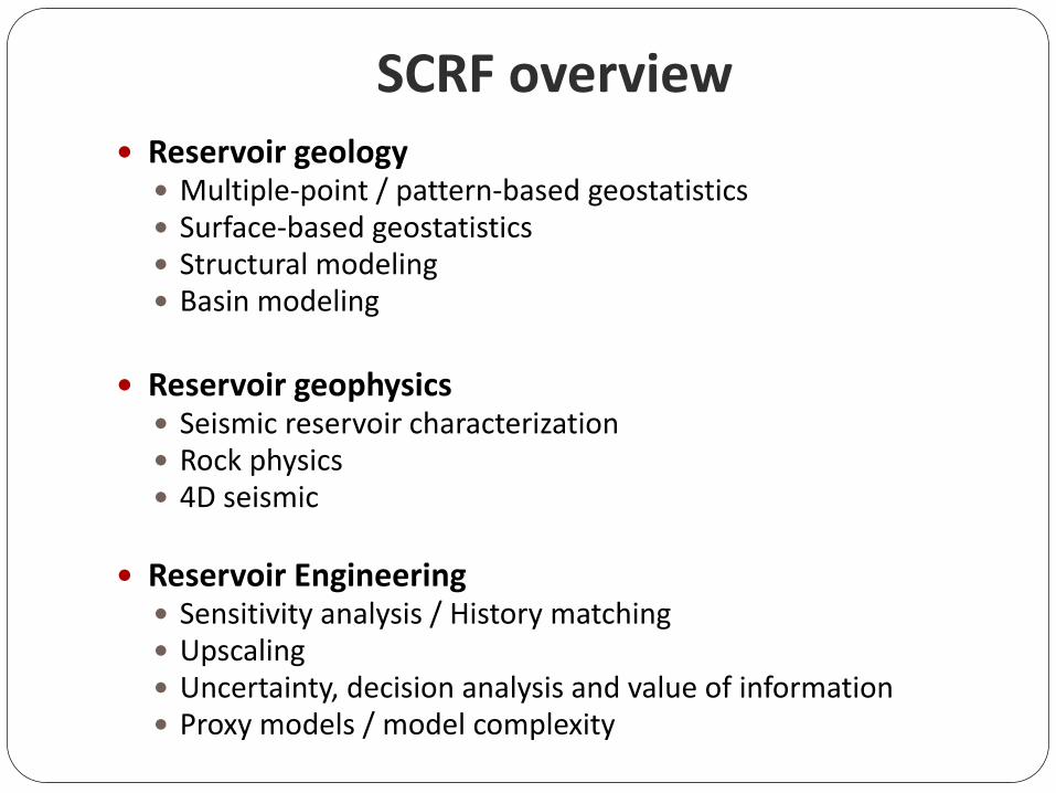
SCRF overview Reservoir geology Multiple-‐point / pattern-‐based geostatistics Surface-‐based geostatistics Structural modeling Basin modeling
Reservoir geophysics Seismic reservoir characterization Rock physics 4D seismic
Reservoir Engineering Sensitivity analysis / History matching Upscaling Uncertainty, decision analysis and value of information Proxy models / model complexity

Jef Caers
Stanford University, USA
Uncertainty, sensitivity and rejection in predictive reservoir modeling

Current practice
Industry practice of
The reservoir
Life-‐tim
e
2D seismic
3D seismic
3D seismic+production
4D seismic+production
sensitivity/rejection
Life-‐tim
e
The reservoir
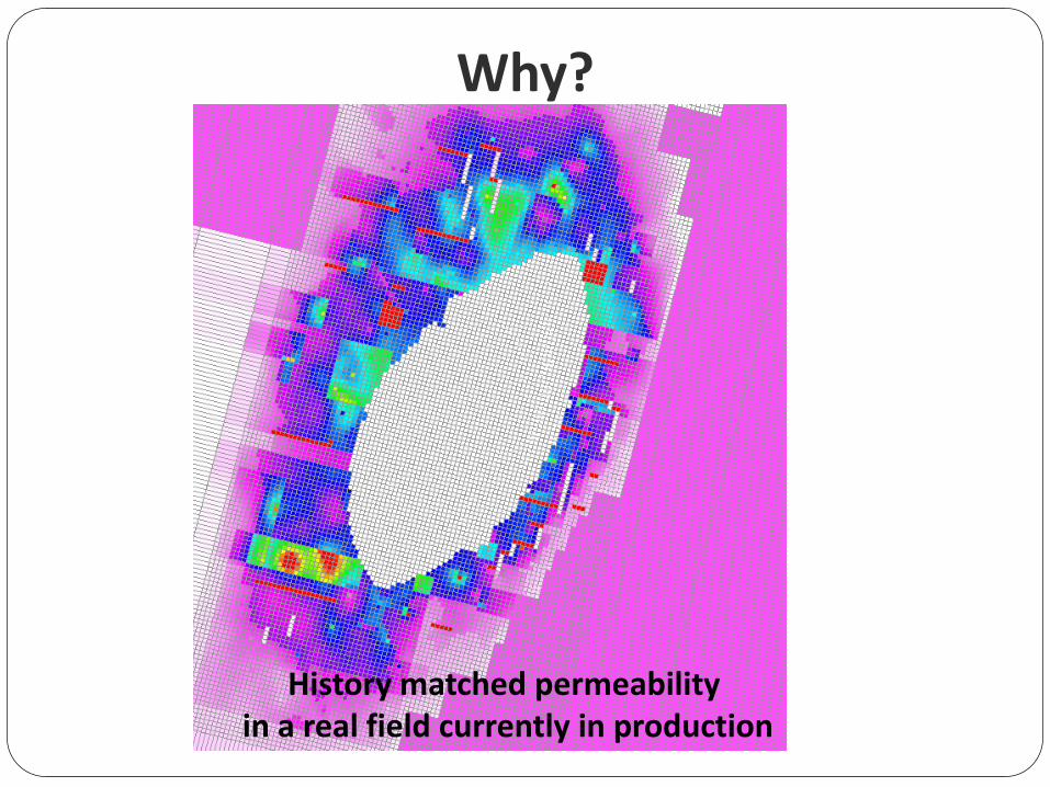
Why?
History matched permeability in a real field currently in production

The sensitivity argument
Any modeling of uncertainty is irrelevant/impossible without a decision or prediction goal Need for an understanding and discovery of what impacts flow processes and decision variables More than just a computational issue !
Challenge: Flow: very non-‐linear process Most important and impacting variables are discrete

The rejection argument
Karl Popper (1959): physical processes are laws that are only abstract in nature and can never be proven correct, they can only be disproven/falsified with facts or data Popper-‐Bayes
(data|m(model|d odel) ata del)) (moPPP

Application to reservoir case study
New well planned
P1
P2
P3
P4
West-‐Coast Africa (WCA) slope-‐valley system
Data courtesy of Chevron

Sensitivity
Depositional model (Training Image) Spatial uncertainty (for given depositional model) Kv/Kh ratio
Residual oil saturation Maximum water relative permeability value Water Corey exponent
What matters for prediction ?

Generalized Sensitivity Analysis (GSA) underlying principle
input parameters
A big modeling box
Geology/geophysics Stochastic
Flow
output response
A measure of sensitivity is the difference between the frequency distributions of input parameters per each class
Dim. Reduction classification
C1 C2 C3
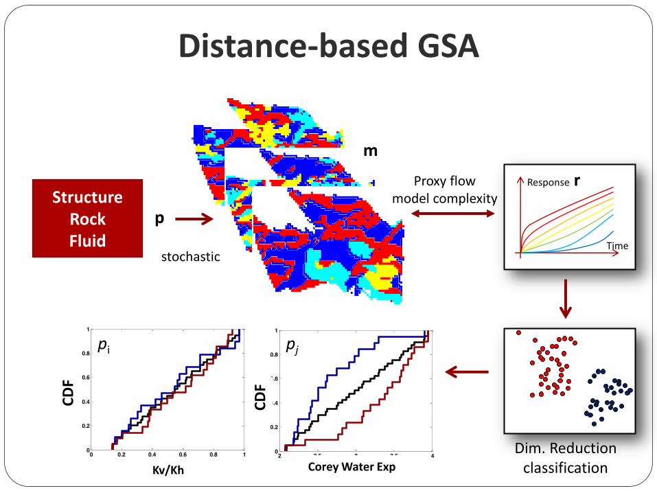
Distance-‐based GSA
Structure Rock Fluid
stochastic
Proxy flow model complexity
Response r
Time
p
m
Dim. Reduction classification
2 2.5 3 3.5 40
0.2
0.4
0.6
0.8
1
watExp
cdf
0 0.2 0.4 0.6 0.8 10
0.2
0.4
0.6
0.8
1
KvKh
cdf
pi pj
CDF
CDF
Kv/Kh Corey Water Exp

Generalized sensitivity any parameter, any response
A measure of sensitivity is the L1 norm difference between a class-‐conditional and marginal cdfs A measure of interaction sensitivity is the L1 norm difference between a conditional class-‐conditional and conditional cdfs
0 0.2 0.4 0.6 0.8 10
0.2
0.4
0.6
0.8
1
x
cdf
( | )i kF p c
( )iF p
pi = corey exponent
TI1 TI3 TI8 TI9 TI10 TI130
0.2
0.4
0.6
0.8
1
TIcd
f
TI|krwMax - class # 1pj = TI ; pi = corey exponent
cdf
( | , )i j kF p p c
( | )i kF p c
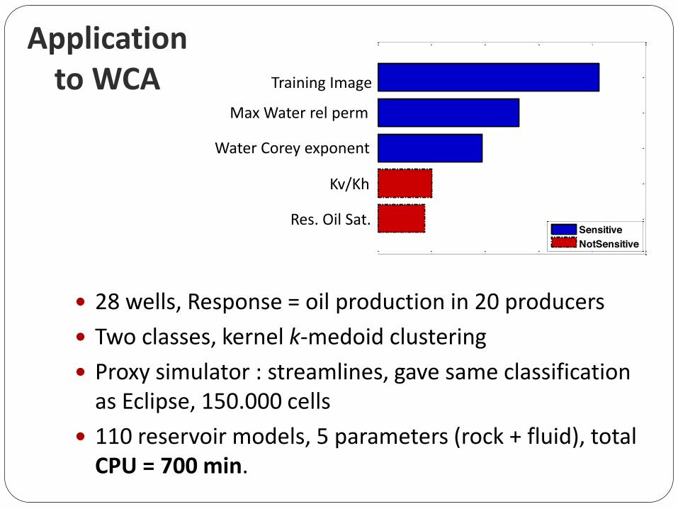
Application to WCA
28 wells, Response = oil production in 20 producers Two classes, kernel k-‐medoid clustering Proxy simulator : streamlines, gave same classification as Eclipse, 150.000 cells 110 reservoir models, 5 parameters (rock + fluid), total CPU = 700 min.
0 0.5 1 1.5 2 2.5
SOWCR
KvKh
TI
krwMax
watExp
SensitiveNotSensitive
Water Corey exponent
Max Water rel perm
Res. Oil Sat.
Training Image
Kv/Kh

Conditional Interaction
0 0.2 0.4 0.6 0.8 1
watExp|KvKhSOWCR|krwMaxkrwMax|SOWCR
krwMax|TITI|watExp
KvKh|watExpTI|KvKh
krwMax|KvKhKvKh|krwMax
watExp|TIKvKh|TI
SOWCR|KvKhwatExp|krwMax
TI|krwMaxSOWCR|watExpwatExp|SOWCR
SOWCR|TITI|SOWCR
krwMax|watExpKvKh|SOWCR
SensitiveNotSensitive
0 0.5 1 1.5 2 2.5
SOWCR
KvKh
TI
krwMax
watExp
SensitiveNotSensitive
TI
Wat exp
Krw Max
KvKh
SOW CR
Interaction is asymmetric one-‐way sensitivity often not fully informative
/r
Kv Kh
/ |r
Kv Kh Sowcr
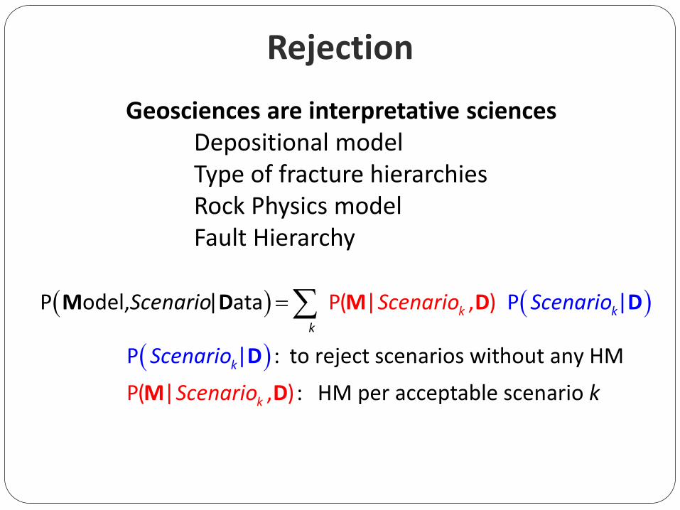
Rejection
P odel, | ata
: to reject scenarios without
P( | , )
any HM: HM per ac
P |
ceptabl P( e scenario P |
| , )
kk
k
k
k
ScenariScenar o
Scenar
io
Sc
Sc
e
e
nar
na
k
io
o
rio
i
M D
MD
M D D
D
Geosciences are interpretative sciences Depositional model Type of fracture hierarchies Rock Physics model Fault Hierarchy

Data: geology and production
TI1: 50% TI2: 25% TI3: 25%
geological scenario
uncertainty: 3 training images
Production Data:
Water rate/well

Two modeling questions
P odel, | ata
: reject data-‐inconsistent training images
: sampling with the remaining ones
P |
P
P( | , )
P( | , )
|
k
k
k
k
k
TI
TI
I
I TIT
T
M DM
D
D D
D
M
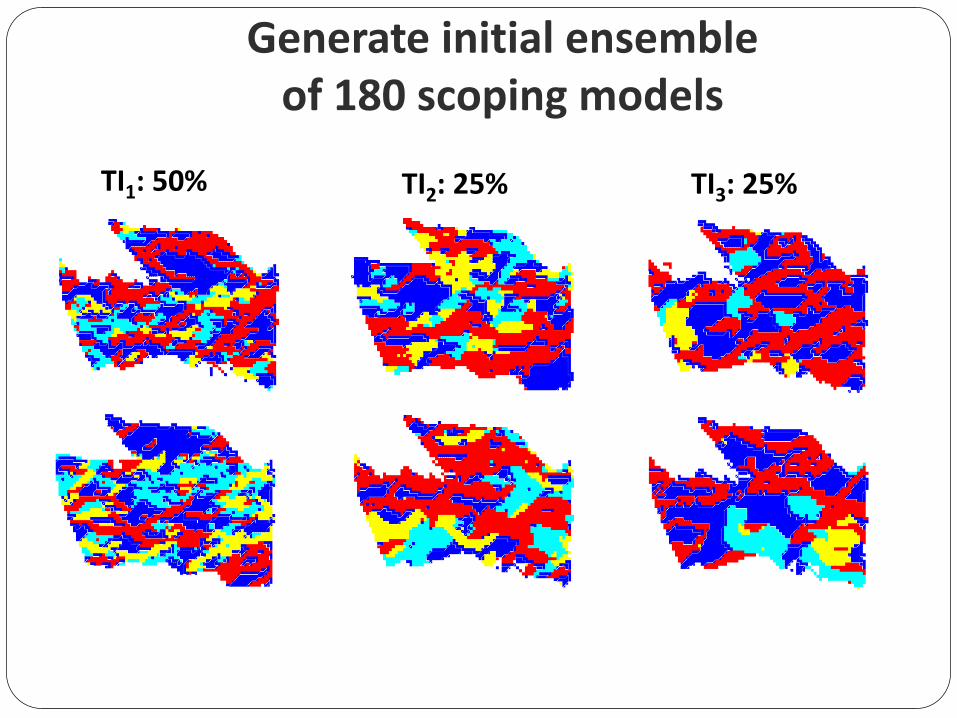
Generate initial ensemble of 180 scoping models
TI1: 50% TI2: 25% TI3: 25%

Production data & 180 Scoping runs Water ra
te
Time/Days
Well 1 Well 2
Well 3 Well 4

Trying to falsify TIs with data represent data in lower dimensions using
multi-‐dimensional scaling
MDS: distance = difference in water rate response for all wells 9 dimensions = 99% of variance
Production data
TI1 responses TI2 responses TI3 responses
Eigencom
pone
nt 2
Eigencomponent 1
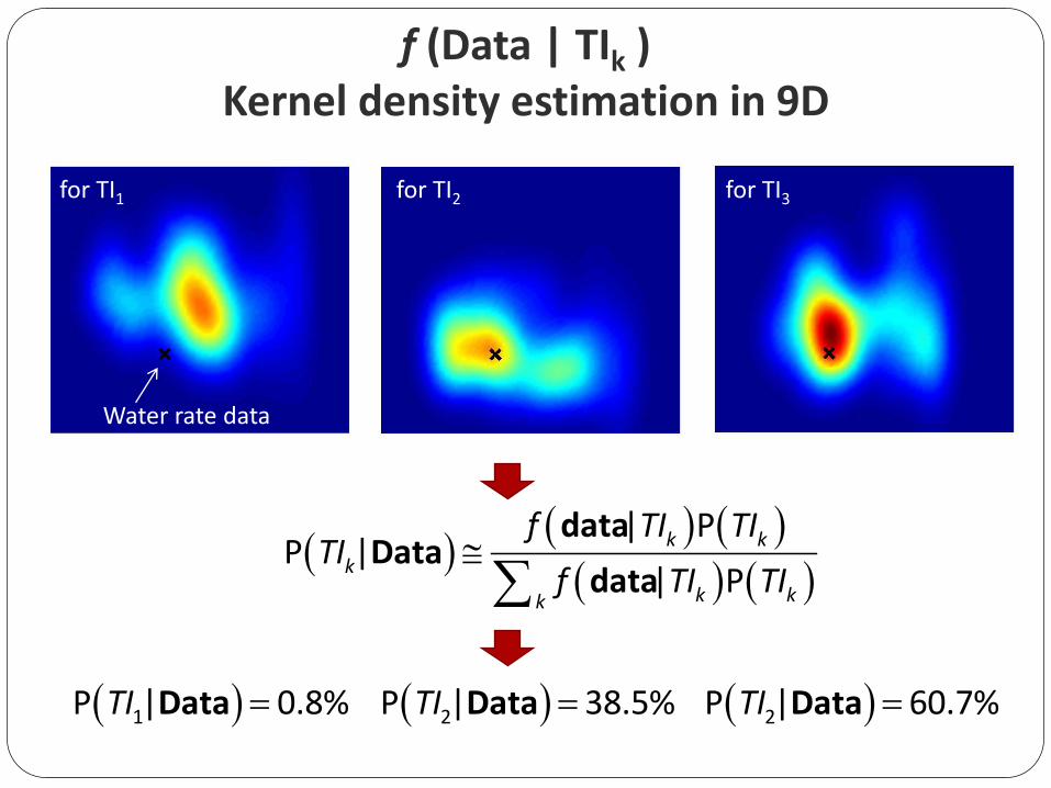
f (Data | TIk ) Kernel density estimation in 9D
| PP |
| Pk k
k
k kk
f TI TITI
f TI TI
dataData
data
1P | 0.8% TI Data 2P | 38.5% TI Data 2P | 60.7% TI Data
for TI1 for TI2 for TI3
Water rate data
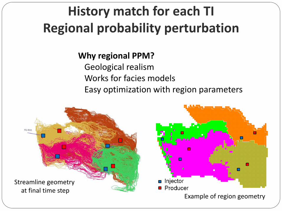
History match for each TI Regional probability perturbation
Why regional PPM? Geological realism Works for facies models Easy optimization with region parameters
Streamline geometry at final time step
Example of region geometry

History match results for all TIs CPU: Average of 24 flow simulations/model
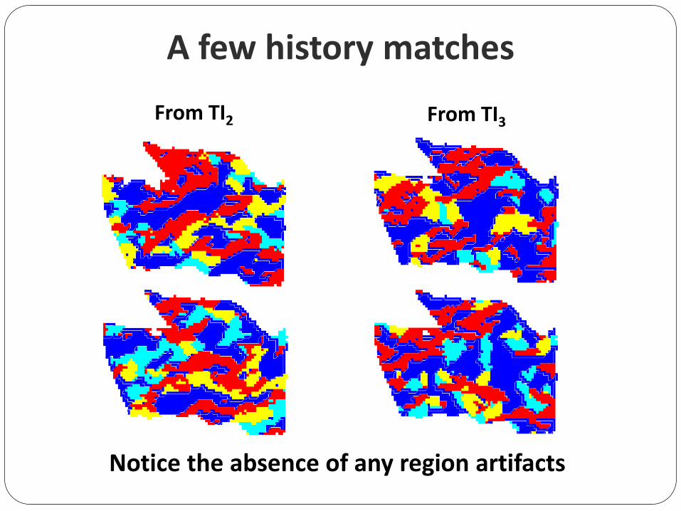
A few history matches
Notice the absence of any region artifacts
From TI2 From TI3

Rejection sampler on TI and facies
1. Draw randomly a TI from the prior
2. Generate a single geo-‐model m with that TI
3. Run the flow model simulator to obtain a response d=g(m)
4. Accept the model using the following probability
2
RMSE( , ( ))exp
2obs gp
d m
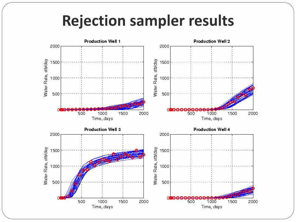
Rejection sampler results
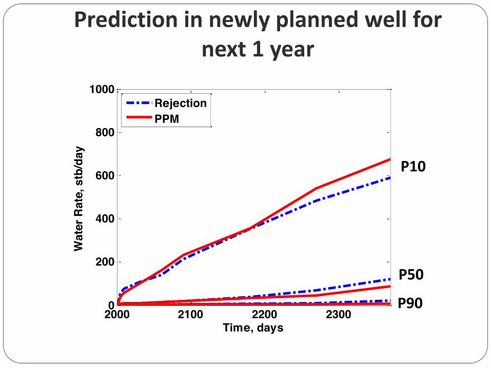
Prediction in newly planned well for next 1 year
2000 2100 2200 23000
200
400
600
800
1000
Time, days
Wat
er R
ate,
stb
/day
RejectionPPM
P10
P50
P90

Comparison
P(TI1|D) P(TI2|D) P(TI3|D) Runs/ model
Method 1% 38% 61% 24
Rejection Sampler 3% 33% 64% 250
Further speed-‐up by realizing that HM per scenario had little impact on reduction of uncertainty use of proxy flow models because only relative likelihood accuracy is needed

Some observations
There is no need for a history match to get a good prediction (this is case dependent)
No need to run full-‐physics on all models Sensitivity: proxies may provide accurate classification Rejection: only relative likelihood is needed
Increased importance on providing geological uncertainty through multiple scenarios
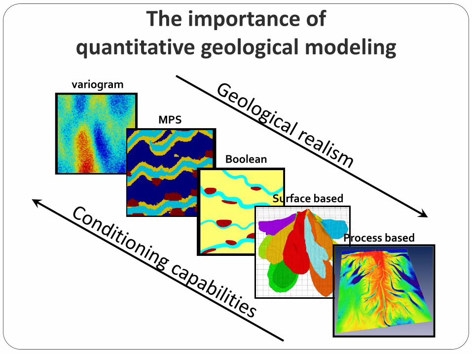
The importance of quantitative geological modeling variogram
MPS
Boolean
Process based
Surface based
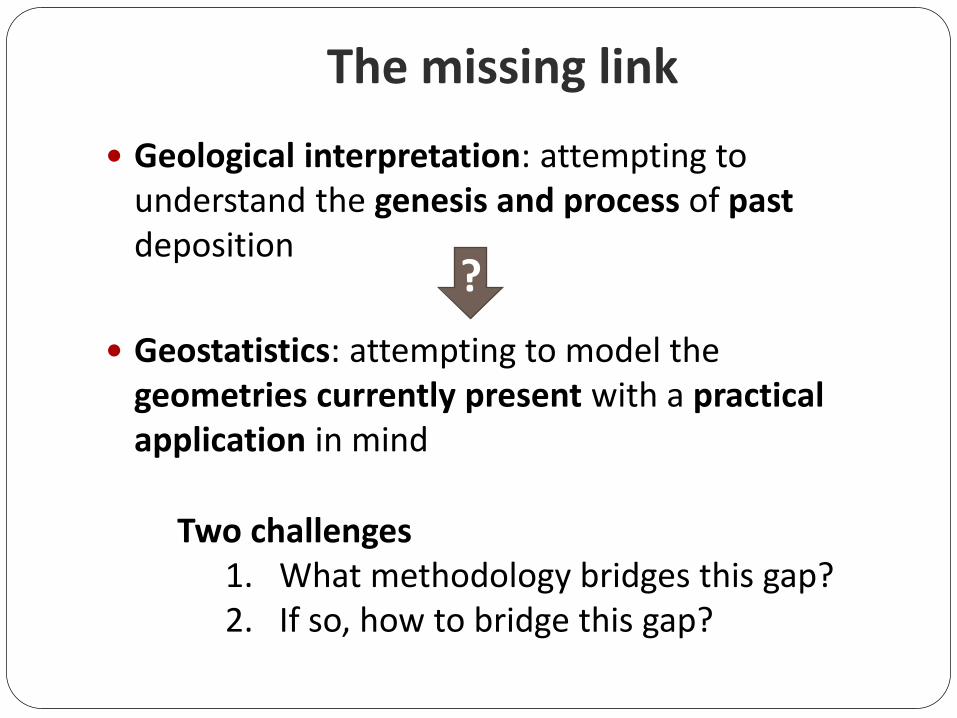
The missing link Geological interpretation: attempting to understand the genesis and process of past deposition Geostatistics: attempting to model the geometries currently present with a practical application in mind
Two challenges 1. What methodology bridges this gap? 2. If so, how to bridge this gap?
?

Limitation of covariances
0.4
0.8
1.2
10 20 30 40 0
0.4
0.8
1.2
10 20 30 40 0
3
1 2
data model
Variograms EW Variograms NS
1 2 3

Training images From Boolean From high resolution seismic
From process-‐based models
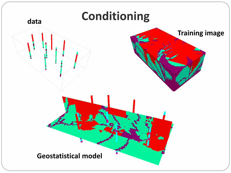
Conditioning data Training image
Geostatistical model
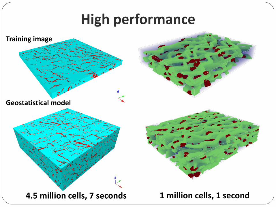
High performance Training image
Geostatistical model
4.5 million cells, 7 seconds 1 million cells, 1 second
Honarkhah, M. and Caers, J. (2012) Math. Geosc., 44:651 672. Direct pattern-‐based simulation of non-‐stationary geostatistical models Pejman Tahmasebi et al. (2012) Comp. Geosc., 16:779 797. Multiple-‐point geostatistical modeling based on the cross-‐correlation functions Fenwick, D., Scheidt, C., and Caers, J. (2012) submitted A distance-‐based generalized sensitivity analysis for reservoir modeling Park, H., Scheidt, C. Fenwick, D. Boucher, A and Caers, J. (2012) submitted History matching and uncertainty quantification of facies models with multiple geological interpretation Scheidt, C., Renard, P and Caers, J. (2012) submitted Uncertainty Quantification in Inverse Problems: Model-‐based versus Prediction-‐Focused Aydin, O. and Caers, J. (2012) submitted Image transforms for determining fit-‐for-‐purpose complexity of geostatistical models in flow modeling PDFs available