Uncertainty Traps∗

Pablo Fajgelbaum

UCLA and NBER

Edouard Schaal

NYU

Mathieu Taschereau-Dumouchel

Wharton

May 10, 2016

Abstract

We develop a theory of endogenous uncertainty and business cycles in which short-lived

shocks can generate long-lasting recessions. In the model, higher uncertainty about fundamen-

tals discourages investment. Since agents learn from the actions of others, information flows

slowly in times of low activity and uncertainty remains high, further discouraging investment.

The economy displays uncertainty traps: self-reinforcing episodes of high uncertainty and low

activity. While the economy recovers quickly after small shocks, large temporary shocks may

have long-lasting effects on the level of activity. The economy is subject to an information

externality but uncertainty traps may remain in the efficient allocation. Embedding the mech-

anism in a standard business cycle framework, we find that endogenous uncertainty increases

the persistence of large recessions and improves the performance of the model in accounting for

the Great Recession.

JEL Classification: E32, D80

∗We thank the editor Robert Barro and two anonymous referees for valuable suggestions. Liyan Shi and ChunzanWu provided superb research assistance. We are grateful to Andrew Abel, Andrew Atkeson, Michelle Alexopoulos,Jess Benhabib, Harold Cole, Michael Evers, Joao Gomes, William Hawkins, Patrick Kehoe, Lars-Alexander Kuehn,Ali Shourideh, Laura Veldkamp, Pierre-Olivier Weill and seminar participants for useful comments. Correspondingauthor: Edouard Schaal, 19 W. 4th Street, 6FL, New York, NY 10012, edouard.schaal@nyu.edu.

1

1 Introduction

We develop a theory of endogenous uncertainty and business cycles. The theory combines two

forces: higher uncertainty about economic fundamentals deters investment, and uncertainty evolves

endogenously because agents learn from the actions of others. The unique rational expectation

equilibrium of the economy features uncertainty traps: self reinforcing episodes of high uncertainty

and low economic activity that cause recessions to persist. Because of uncertainty traps, large but

short-lived shocks can generate long-lasting recessions. We first build and characterize a model

that only includes the essential features that give rise to uncertainty traps. Then, we embed

these features into a standard real business cycle model and quantify the impact of endogenous

uncertainty during the Great Recession.

In the model, firms decide whether to undertake an irreversible investment whose return depends

on an imperfectly observed fundamental that evolves randomly according to a persistent process.

Firms are heterogeneous in the cost of undertaking this investment and hold common beliefs about

the fundamental. Beliefs are regularly updated with new information, and, in particular, firms

learn by observing the return on the investment of other producers. We define uncertainty as the

variance of these beliefs.

This environment naturally produces an interaction between beliefs and economic activity.

Firms are more likely to invest if their beliefs about the fundamental have higher mean, but also if

they have smaller variance (lower uncertainty). At the same time, the laws of motion for the mean

and variance of beliefs depend on the investment rate. In particular, when few firms invest, little

information is released, so uncertainty rises.

The key feature of the model is that this interaction between information and investment leads to

uncertainty traps, formally defined as the coexistence of multiple stationary points in the dynamics

of uncertainty and economic activity. Without shocks, the economy converges to either a high

regime (with high economic activity and low uncertainty) if the current level of uncertainty is

sufficiently low, or to a low regime (with low activity and high uncertainty) if the current level of

uncertainty is sufficiently high. Because of the presence of these multiple stationary points, the

economy exhibits non-linearities in its response to shocks: starting from the high regime, it quickly

recovers after small temporary shocks, but it may shift to the low-activity regime after a large

temporary shock. Once it has fallen in the low regime, only a large enough positive shock can push

the economy back to the high-activity regime.

An important feature of the model is that, despite the presence of uncertainty traps, there is a

unique recursive competitive equilibrium. That is, multiplicity of stationary points does not mean

multiplicity of equilibria. Therefore, unlike other macro models with complementarities, there is

no room in our model for multiple equilibria or sunspots.1

The model features an inefficiently low level of investment because agents do not internalize the

effect of their actions on public information. This inefficiency naturally creates room for welfare-

1For recent examples of business cycle models with multiple equilibria see Farmer (2013), Kaplan and Menzio(2013), Benhabib et al. (2015) and Schaal and Taschereau-Dumouchel (2015).

2

enhancing policy interventions. We therefore study the problem of a constrained planner that is

subject to the same informational constraints as private agents. The socially constrained-efficient

allocation can be implemented with a subsidy to investment. But, perhaps surprisingly, the optimal

policy does not necessarily eliminate uncertainty traps. Therefore, while policy interventions are

desirable, they do not eliminate the adverse feedback loop between uncertainty and economic

activity.

To evaluate the quantitative implications of uncertainty traps, we embed the key features of

the baseline model into a standard general equilibrium framework and then compare its predictions

with an RBC model and the data. To isolate the impact of endogenous movements in uncertainty,

we also compare our full model to a “fixed θ-uncertainty” version in which uncertainty about the

fundamental productivity θ is fixed over time. We discipline the key parameters of the model, those

that determine option-value effects and the evolution of uncertainty, by targeting moments from

the distribution of uncertainty about real GDP growth from the Survey of Professional Forecasters

(SPF).

We first show that our calibrated model performs as well as the RBC and fixed θ-uncertainty

models in terms of traditional business cycle moments. Therefore, incorporating endogenous uncer-

tainty in a standard business cycle model does not impair its ability to predict well-known patterns

of business cycle data.

Then, we demonstrate that the non-linearities generated by uncertainty traps, studied in the

baseline theory, are active in the calibrated model. Specifically, we compute the economy’s response

to one-period negative shocks to beliefs of different magnitudes. We find that i) recessions are longer

and deeper under the full model than under the fixed θ-uncertainty model, and ii) the difference

between both models is more important for large shocks than for small ones. In response to a

-1% shock, the ensuing recession is 22% deeper (in terms of the peak-to-trough fall in output) and

40% longer (in terms of quarters until the economy has recovered half of the peak-to-trough fall

in output) in the full model than in the fixed θ-uncertainty model. However, in response to a

larger -5% shock, the recession is 35% deeper and 66% longer in the full model than in the fixed

θ-uncertainty model. Therefore, in the calibrated model, the endogenous uncertainty mechanism,

whose impact is captured by the difference between the full and fixed θ-uncertainty models, makes

recessions deeper and longer for shocks of any magnitude, but relatively more so for larger shocks.

Finally, our main quantitative exercise evaluates the predictions of our calibrated model for past

U.S. recessions. Since our mechanism provides amplification and persistence to large shocks, we

expect that it might help explain particularly severe recessions observed in the data. We therefore

investigate the largest recession in our sample, the Great Recession. To do so, we feed each of

the three models (our full model, the RBC model, and the fixed θ-uncertainty model) with the

observed TFP series and signals such that each model replicates the time series of forecasts about

output growth from the SPF during the first part of the recession. We then contrast each model’s

response with the data.

Our main quantitative finding is that, during the Great Recession, our model generates declines

3

in output, consumption, employment, and investment which are clearly more protracted, and closer

to patterns observed in the data, than what the alternative models predict. Endogenous uncertainty

adds 1.8 percentage points in terms of recession’s depth and slows the recovery by about two years

relative to the fixed θ-uncertainty model.2 The corresponding numbers are 5.2 percentage points

and five years when comparing to the RBC model. We also evaluate the performance of the three

models against the data in terms of one key statistic that summarizes both the depth and the

length of the recession: the cumulative output loss between the start of the recession and 2015. We

find that our model generates 93% of the Great Recession’s cumulative output lost, relative to the

70% and 30% generated by the fixed θ-uncertainty and RBC models, respectively. Reassuringly,

the model also generates patterns for the evolution of uncertainty about output growth that are

roughly consistent with the data.

We demonstrate the robustness of these conclusions by replicating this exercise under alterna-

tive assumptions about the shocks hitting the economy, the source of the TFP data, the detrending

strategy, and the preferences of the household. In each case, we find that the model with endoge-

nous uncertainty performs better than its alternatives. To make sure that the full model does not

generate counterfactual amounts of persistence for milder recessions, we also replicate the second

largest recession in our sample, the 1981-1982 recession, which was characterized by a relatively

rapid recovery. We find that our model behaves similarly to the RBC and to the fixed θ-uncertainty

models in that case. We conclude that the inclusion of uncertainty traps in a standard macroeco-

nomic model of business cycles improves its performance during the Great Recession and that it

leads to similar predictions than standard models for smaller recessions.

The remainder of the introduction contains the literature review followed by a discussion of our

notion of uncertainty and its business cycle properties. The paper is then structured as follows.

Section 2 presents the baseline model and the definition of the recursive equilibrium. Section 3

characterizes the investment decision of an individual firm and demonstrates the existence and

uniqueness of the equilibrium. Section 4 shows the existence of uncertainty traps, examines the

non-linearities that they generate, and characterizes the planner’s problem. Section 5 describes the

quantitative model, shows how uncertainty traps influence the response of the economy to shocks

and compares the dynamic properties of our model to an RBC model, a fixed θ-uncertainty model

and the data over the Great Recession. Section 6 concludes. The full statement of the proposition

and the proofs can be found in the appendix.

1.1 Relation to the Literature

The theory is motivated by an empirical literature that investigates the impact of uncertainty

on economic activity using VARs, as in Bloom (2009) and Bachmann et al. (2013), or using in-

strumental variables, as in Carlsson (2007), and finds that increases in uncertainty typically slow

2This measure refers to the time the economy takes to recover 20% of its peak-to-trough decline. We use the20% threshold instead of the usual half-life since, in the data, detrended output has only recovered about 20% of itspeak-to-trough decline by the end of our sample in 2015.

4

down economic activity. It also relates to the uncertainty-driven business cycle literature that ana-

lyzes the impact of uncertainty through real option effects as in Bloom (2009), Bloom et al. (2012),

Bachmann and Bayer (2013) and Schaal (2015), or through financial frictions as in Arellano et al.

(2012) and Gilchrist et al. (2014).3

Our analysis also relates to a theoretical literature in macroeconomics that stud-

ies environments with learning from market outcomes such as Veldkamp (2005), Ordonez

(2009) and Amador and Weill (2010). Closely related to our paper is the analysis of

Van Nieuwerburgh and Veldkamp (2006). They focus on explaining business-cycle asymmetries

in an RBC model with incomplete information in which agents receive signals with procyclical pre-

cision about the economy’s fundamental. During recessions, agents discount new information more

heavily and the mean of their beliefs recovers slowly. Their paper provides a theory of endogenous

pessimism that can explain business cycle asymmetries. Our model introduces a similar learning en-

vironment in a model of irreversible investment under uncertainty in the spirit of Dixit and Pindyck

(1994) and Stokey (2008). The resulting feedback loop between endogenous uncertainty and real

option effects, specific to our approach, offers a novel propagation mechanism that can lead to

persistent episodes of high uncertainty and low economic activity.

The interaction of endogenous uncertainty and real option effects in our model is also reminiscent

of the literature on learning and strategic delays as in Lang and Nakamura (1990), Rob (1991),

Caplin and Leahy (1993), Chamley and Gale (1994), Zeira (1994) and Chamley (2004). Our paper

differs from this literature in its attempt to evaluate and quantify the role of uncertainty and delays

in a standard business cycle framework. In a recent paper in which learning and economic activity

interact, Straub and Ulbricht (2015) propose a theory of endogenous uncertainty in which financial

constraints impede learning about firm-level fundamentals. Financial crises cause uncertainty to

rise, leading to a further tightening of financial constraints that amplifies and propagates recessions.4

In another recent paper considering the role of learning during the Great Recession, Kozlowski et al.

(2015) suggest that the Great Recession was the result of an unlikely shock that caused agents to

substantially revise their beliefs about the probability of lower-tail events. They find that the

resulting increase in pessimism may account for part of the long-lasting downturn.

This paper is also related to the literature on fads and herding in the tradition of Banerjee (1992)

and Bikhchandani et al. (1992) . Articles in that tradition consider economies with an unknown

fixed fundamental and study a one-shot evolution towards a stable state, whereas we study the full

cyclical dynamics of an economy that fluctuates between regimes.

The dynamics generated by the model, with endogenous fluctuations between regimes, is remi-

niscent of the literature on static coordination games such as Morris and Shin (1998, 1999) and the

dynamic coordination games literature as Angeletos et al. (2007) and Chamley (1999). These pa-

pers study games in which a complementarity in payoffs leads to multiple equilibria under complete

3Another literature studying time-varying risk is the literature on rare disasters (Barro, 2006) and time-varyingdisaster risk as in Gabaix (2012) and Gourio (2012), and surveyed in Barro and Ursua (2012).

4Some recent papers discuss alternative channels that give rise to endogenous volatility over the business cycle.See Bachmann and Moscarini (2011) and Decker and D’Erasmo (2016).

5

information. The introduction of strategic uncertainty through noisy observation of the fundamen-

tal leads to a departure from common knowledge that eliminates the multiplicity. In contrast, the

complete-information version of our model does not feature multiplicity, and complementarity only

arises under incomplete information through social learning. Uniqueness does not obtain through

strategic uncertainty, but by limiting the strength of the complementarities.

1.2 Bayesian Uncertainty and the Business Cycle

Throughout the paper, we adopt the concept of Bayesian uncertainty : in our theory, all agents

have access to the same information It at time t and use Bayes’ rule to form beliefs about the fun-

damental of the economy θt, which is, in our context, the aggregate productivity process. We define

uncertainty as the variance Var (θt | It) of the probability distribution that describes these com-

mon beliefs. In contrast, the uncertainty-driven business cycle literature that we referenced above

defines uncertainty as time-varying volatility in exogenous aggregate or idiosyncratic variables.

These two definitions of uncertainty are related, but they are not identical. They are related

because time-varying volatility may generate uncertainty about the future fundamentals of the

economy, giving rise to Bayesian uncertainty. However, they are different because Bayesian uncer-

tainty may fluctuate without the presence of time-varying volatility. In our model, the variance of

beliefs varies over time through learning, while the volatility of exogenous variables is constant.

A basic and well known feature of the data which motivates our theory is that uncertainty

increases during recessions. Instead of direct measures of time-varying volatility, we present, in

Figure 1 , the evolution of four measures that capture our notion of Bayesian uncertainty to the

extent that they reflect uncertainty in subjective beliefs.5 Panel (a) shows the VXO, a measure

of stock market volatility as perceived by market participants; Panel (b) shows the uncertainty

measure proposed by Jurado et al. (2015), which captures a Bayesian notion of ex-ante forecast

error in a statistical model of the macroeconomy; Panel (c) shows the standard deviation of the

average perceived distribution of output growth from the Survey of Professional Forecasters (SPF);

and Panel (d) shows the fraction of respondents who answer “uncertain future” as a reason for why

it is a bad time to buy major household goods from the Michigan Survey of Consumers. While these

series attempt to measure distinct objects, they all capture the notion of subjective uncertainty.

All these measures support the key implication of our mechanism, that uncertainty rises during

recessions. In the quantitative section of the paper, we use the SPF measure to calibrate and

evaluate the performance of our model because it has a natural counterpart in our framework.

5The uncertainty-driven business cycle literature measures aggregate uncertainty by the conditional heteroskedas-ticity of various aggregates such as TFP (Bloom et al., 2012). Time-varying volatility in idiosyncratic variables istypically proxied by cross-sectional dispersions in sales growth rates (Bloom, 2009), output and productivity (Kehrig,2011), prices (Vavra, 2014), employment growth (Bachmann and Bayer, 2014), or business forecasts (Bachmann et al.,2013). All these measures have been shown to be countercyclical. Since all agents have the same beliefs about θ,these cross-sectional measures are uninformative about uncertainty in our model.

6

0

10

20

30

40

50

60

70

1990 1995 2000 2005 2010

0.8

0.9

1

1.1

1.2

1.3

1970 1980 1990 2000 2010

0.8

0.9

1

1.1

1.2

1.3

1.4

1.5

1.6

1995 2000 2005 2010 2015

0

5

10

15

20

25

1970 1980 1990 2000 2010

(a) VXO (b) Jurado et al. (2015)

(c) SPF (d) Michigan Survey

Notes: (a) The CBOE’s VXO series is a measure of market expectations of stock market volatility over the next 30 daysconstructed from S&P100 option prices. We present monthly averages of the series over 1986-2014. (b) Jurado et al. (2015)estimate a large-scale structural model with time-varying volatility on the US economy and use it compute an implied measureof ex-ante forecast error. The series we present corresponds to the H12 measure, i.e., an equal-weighted average of the 12-monthahead standard deviations over 132 macroeconomic series. (c) The SPF series is the standard deviation of the “mean probabilityforecast”: an average of the probability distribution provided over forecasters, of one-year ahead output growth in percentageterms. (d) The Michigan Survey series correspond to the percent fraction of all respondents that reply “uncertain future” tothe question why people are not buying large household items. Shaded areas correspond to NBER recessions.

Figure 1: Various measures of subjective uncertainty

7

2 Baseline Model

We begin by presenting a stylized model that only features the necessary ingredients to generate

uncertainty traps. The intuitions from this simple model as well as the laws of motion governing the

dynamics of uncertainty carry through to the extended model that we use for numerical analysis.

2.1 Population and Technology

Time is discrete. There is a fixed number of firms N , chosen large enough that firms behave

atomistically. Each firm j ∈

1, . . . , N

holds a single investment opportunity that produces output

θ, common to all firms. We refer to θ as the economy’s fundamental. and assume that it follows

the autoregressive process

θ′ = ρθθ + εθ, εθ ∼ iid N(

0,(

1− ρ2θ)

σ2θ)

, (1)

where 0 < ρθ < 1 is the persistence of the process and σ2θ the variance of its ergodic distribution.

To produce, a firm must pay a fixed cost f , drawn each period from the continuous cumulative

distribution F with mean µf and standard deviation σf . Once production has taken place, the firm

exits the economy and is immediately replaced by a new firm holding an investment opportunity.

This assumption ensures that the mass of firms in the economy remains constant.6

Upon investment, the firm receives the payoff θ. Firms have constant absolute risk-aversion,7

u (θ) =1

a

(

1− e−aθ)

,

where a > 0 is the coefficient of absolute risk aversion.

2.2 Timing and Information

Firms do not know the true value of the fundamental θ and decide whether to invest or not

based on their beliefs. As time unfolds, they learn about θ in various ways. First, they learn from

a public signal Z with precision γz > 0 observed at the end of each period,

Z = θ + εZ , εz ∼ iid N (0, γ−1z ). (2)

This signal captures the information released by statistical agencies or the media. Second, agents

acquire information through social learning. When firm j invests, a noisy signal about its return,

xj = θ + εxj , is sent to all firms.8 The noise εxj is normally distributed with precision γx/N > 0,

6This assumption is made for tractability and is relaxed in the quantitative section.7Here, agents can be thought of as entrepreneurs with risk averse preferences. In our quantitative model, firms

use the representative household’s stochastic discount factor.8Social learning captures the idea that firms learn from each other about various common components that affect

their revenues such as productivity, demand, regulations, etc. Social learning has been found to influence economicdecisions in various contexts. Foster and Rosenzweig (1995) estimate a model of the adoption of high-yielding seedsin India and find it consistent with social learning. Guiso and Schivardi (2007) find that peer-learning effects matter

8

independent over time and across investors, but common to all observers.9 We denote by N ∈

0, . . . , N

the endogenous number of firms that invest and n = N/N the fraction of investing

firms. Because of the normality assumption, a sufficient statistic for the information provided by

investing firms is the public signal

X ≡ 1

N

∑

j∈I

xj = θ + εXN , (3)

where I is the set of such firms, and

εXN ≡ 1

N

∑

j∈I

εxj ∼ N(

0, (nγx)−1)

.

Importantly, the precision nγx of this signal increases with the fraction of investing firms n.

The timing of events is summarized in Figure 2.

N firms decide to investbased on beliefs and

investment costs

Production takes place;Public signals X and Z

are observed

Beliefs are updated

...t+1t

Figure 2: Timing of events

2.3 Beliefs

Under the assumption of a common initial prior, and because all information is public, beliefs are

common across firms. In particular, there is no cross-sectional dispersion in beliefs. The normality

assumptions about the signals and the fundamental imply that beliefs are also normally distributed

θ | I ∼ N(

µ, γ−1)

,

where I is the information set at the beginning of the period. The mean of the distribution µ

captures the optimism of agents about the state of the economy, while γ represents the precision of

their beliefs about the fundamental. Precision γ is inversely related to the amount of uncertainty.

As γ increases, the variance of beliefs decreases, and uncertainty declines.

Firms start each period with beliefs (µ, γ) and use all the information available to update their

beliefs. By the end of the period, they have observed the public signals X and Z. Therefore, using

Bayes’ rule, the beliefs about next period’s fundamental θ′ are normally distributed with mean and

for the behavior of Italian industrial firms. Bikhchandani et al. (1998) survey the empirical social learning literature.9We assume that the precision of each individual signal xj is inversely proportional to N to prevent the signals

to be fully revealing when we take the limit N → ∞, while preserving the positive relationship between economicactivity and the amount of information. This captures the idea that uncertainty may subsist even when the numberof firms is large, either because their information is correlated and arises from the same sources, or because largeeconomies are more complex and subject to more shocks, preventing the learning problem from becoming trivial.

9

precision equal to

µ′ = ρθγµ+ γzZ + nγxX

γ + γz + nγx, (4)

γ′ =

(

ρ2θγ + γz + nγx

+(

1− ρ2θ)

σ2θ

)−1

≡ Γ (n, γ) . (5)

These standard updating rules have straightforward interpretations: the mean of future beliefs µ′

is a precision-weighted average of the present belief µ and the new signals, X and Z, whereas γ′

depends on the precision of current beliefs, the precision of the signals, and the variance of the

shock to θ. Importantly, the precision of future beliefs does not depend on the realization of the

public signals, but only on n and γ. The higher is n, the more precise is the public signal X, and

the lower is uncertainty in the next period. We define Γ (n, γ) in (5) as the law of motion of the

precision of information.

2.4 Firm Problem

We now describe the problem of a firm. In each period, given its individual fixed cost f and

the common beliefs about the fundamental, a firm can either wait or invest. It solves the Bellman

equation

V (µ, γ, f) = max

V W (µ, γ) , V I (µ, γ)− f

, (6)

where V W (µ, γ) is the value of waiting and V I (µ, γ) is the value of investing after incurring the

investment cost f .

If a firm waits, it starts the next period with updated beliefs (µ′, γ′) about the fundamental

and a new draw of the fixed cost f ′. Therefore, the value of waiting is

V W (µ, γ) = βE

[ˆ

V(

µ′, γ′, f ′)

dF(

f ′)

| µ, γ]

. (7)

In turn, upon investment, a firm receives output θ and exits the economy. Therefore,

V I (µ, γ) = E [u (θ) | µ, γ] = 1

a

(

1− e−aµ+a2

2γ

)

. (8)

The firm’s optimal investment decision takes the form of a cutoff rule f c (µ, γ) such that a firm

invests if and only if f ≤ f c (µ, γ). The cutoff is defined by the following indifference condition

f c (µ, γ) = V I (µ, γ)− V W (µ, γ) . (9)

10

2.5 Law of Motion for the Number of Investing Firms N

We now aggregate the individual decisions of the firms. As the investment decision follows the

cutoff rule f c (µ, γ), the process for the number of investing firms N satisfies

N(

µ, γ, fj1≤j≤N)

=

N∑

j=1

1I (fj ≤ f c (µ, γ)) . (10)

Since investment depends on a random fixed cost, the number of investing firms is a random

variable that depends on the realization of the shocks fj1≤j≤N . As these costs are i.i.d., the

ex-ante probability of investment is identical across firms and equal to F (f c (µ, γ)). Therefore, the

ex-ante distribution of N , as perceived by firms, is binomial,

N | µ, γ ∼ Bin(

N,F (f c (µ, γ)))

. (11)

Note that N is only a function of the beliefs (µ, γ) and the individual shocks fj1≤j≤N . Since

these shocks are independent from the fundamental θ and the investment decisions are made before

the observation of returns, there is nothing to learn from the non-investment of firms, nor from the

realization of N itself.

2.6 Recursive Competitive Equilibrium

Focusing on the limiting case when N → ∞, the fraction of investing firms n becomes deter-

ministic,

n =N

N

a.s−→ F (f c (µ, γ)) .

We define a recursive competitive equilibrium as follows.10

Definition 1. A recursive competitive equilibrium consists of a cutoff rule f c (µ, γ), value functions

V (µ, γ, f), V W (µ, γ), V I (µ, γ), laws of motions for aggregate beliefs µ′, γ′, and a fraction of

investing firms n (µ, γ) , such that

1. The value function V (µ, γ, f) solves (6), with V W (µ, γ) and V I (µ, γ) defined according to

(7) and (8), yielding the cutoff rule f c (µ, γ) in (9);

2. The aggregate beliefs (µ, γ) evolve according to (4) and (5), under the perceived fraction of

investing firms n (µ, γ) = F (f c (µ, γ)).

10Fluctuations in N due to finite sampling are irrelevant for our purpose. Our results nonetheless carry on to thefinite N case. Our existence and uniqueness proof for that case is available upon request.

11

3 Equilibrium Characterization

We first characterize the evolution of beliefs. We then show the existence and uniqueness of an

equilibrium, and provide conditions under which firms are less likely to invest when uncertainty is

high.

3.1 Evolution of Beliefs

The optimal investment rule f c (µ, γ) depends on how beliefs evolve. We begin by establishing

two simple lemmas about the dynamics of aggregate beliefs.

3.1.1 Evolution of the Mean of Beliefs

Using (4), we can characterize the stochastic process for the mean of beliefs as follows.

Lemma 1. For a given n, the mean of beliefs µ follows an autoregressive process with time-varying

volatility s,

µ′

= ρθµ+ s (n, γ) ε,

where s (n, γ) = ρθ

(

1γ − 1

γ+γy+nγx

)12and ε ∼ N (0, 1).

The mean of beliefs captures the optimism of agents about the fundamental and evolves stochas-

tically due to the the arrival of new information. It inherits the autoregressive property of the fun-

damental, and its volatility s (n, γ) is time-varying because the amount of information that firms

collect over time is endogenous. The volatility is decreasing with γ and increasing with n. In times

of low uncertainty (γ high) agents place more weight on their current information and less on new

signals, making the mean of beliefs more stable. In contrast, in times of high activity (n high) more

information is released, making beliefs more likely to fluctuate.

3.1.2 Evolution of Uncertainty

The precision of beliefs γ reflects the inverse of uncertainty about the fundamental and its

dynamics play a key role for the existence of uncertainty traps. Its law of motion satisfies the

following properties.

Lemma 2. The law of motion Γ (n, γ) increases with n and γ. For a given fraction of investing

firms n, the law of motion for the precision of beliefs γ′ = Γ (n, γ) admits a unique stable stationary

point in γ.

The thin solid curves on Figure 3 depict Γ (n, γ) for different constant values of n. An increase

in the level of activity raises the next period precision of information γ′ for each level of γ in the

current period. Since n is between 0 and 1, the support of the ergodic distribution of γ must lie

between the bounds γ and γ defined by γ ≡ Γ(0, γ) and γ ≡ Γ(1, γ). In other words, γ is the

stationary level of precision when no firm invests, while γ is the one when all firms invest.

12

0

0.2

0.4

0.6

0.8

1

0 0.2 0.4 0.6 0.8 1

γ′

γ

γ

γ

n = 0

n = 0.5

n = 1

Γ(

n(µ, γ), γ)

Figure 3: Example of dynamics for beliefs precision γ

In equilibrium, n varies with µ and γ. Suppose, as an example, that n is an increasing step

function of γ that takes the values 0, 0.5 or 1, and let us keep µ fixed for the moment. Figure 3

illustrates how the feedback from uncertainty to investment opens up the possibility of multiple

stationary points in the dynamics of the precision of beliefs, and therefore uncertainty. In this

example, the function γ′ = Γ (n (µ, γ) , γ), depicted by the solid curve, has three fixed points. We

formally establish, in Section 4, that this type of multiplicity can happen in equilibrium.

3.2 Existence and Uniqueness

We have described in Lemmas 1 and 2 how beliefs depend on the fraction of investing firms. We

now characterize the equilibrium decision rule and provide existence and uniqueness conditions.

Proposition 1. Under Assumptions 1-3, stated in Appendix F, and for γx sufficiently small, the

equilibrium exists and is unique. Under some additional conditions satisfied when γx is small and

risk aversion “a” is large enough, the equilibrium cutoff f c is increasing in µ and γ.

This proposition establishes the monotonicity of the equilibrium cutoff rule. Anticipating higher

returns, a more optimistic firm (higher µ) is more likely to invest. In turn, uncertainty (lower γ)

reduces the incentives to invest for two reasons. First, risk averse firms dislike uncertain payoffs.

Second, since investment is costly and irreversible, there is an option value of waiting: in the face of

uncertainty, firms prefer to delay investment to gather additional information and avoid downside

risk.

It is essential for our mechanism that uncertainty discourages investment, a feature typical

13

of optimal stopping time models of investment. Assumption 3, satisfied if the persistence of the

fundamental is high enough and its volatility is sufficiently low, ensures that the fundamental does

not vary too much over time, so that firms have an incentive to wait in order to collect more

information.11 This condition alone, however, is not sufficient in our context. The monotonicity

of the cutoff f c in γ requires additional restrictions because of the endogeneity of beliefs, which

gives rise to ambiguous feedback effects. For instance, the variation in n implied by fluctuations

in µ or γ affect the volatility of next period’s mean beliefs µ’ (Lemma 1). This, in turn, can have

ambiguous effects on firms’ current incentives to invest. To ensure that the first-order effects of

risk aversion and option value dominate, we must bound these feedback effects. Since they operate

solely through social learning, we can do so by imposing an upper bound on the informativeness of

this channel, γx. When γx is small enough, the equilibrium cutoff is guaranteed to be increasing in

µ and γ, as one would expect in the absence of social learning.

Establishing the existence of an equilibrium is relatively straightforward, because the problem

is continuous and general fixed point theorems apply. Showing uniqueness is more challenging

because our economy features complementarities in information: the more firms invest, the more

uncertainty declines, encouraging further investment. If these complementarities are strong enough,

they can lead to multiple equilibria. To prevent this, we use again the insight that the magnitude of

this feedback is governed by the precision γx of the social learning channel. We show, in particular,

that the main fixed point problem that characterizes the optimal cutoff rule is a contraction, and

that it is therefore unique, when γx is small.12 The uniqueness of the equilibrium is an attractive

feature, as it leads to unambiguous predictions and makes the model amenable to quantitative work.

Despite the uniqueness of the equilibrium, the model features interesting non-linear dynamics and

multiple stationary points, as we show in Section 4.

Figure 4 illustrates how the investment probability varies as a function of beliefs (µ, γ) when

monotonicity obtains. The fraction of investing firms increases as they are more optimistic (µ high)

or less uncertain (γ high) about the fundamental.

11The law of motion (5) highlights the importance of the persistence of the fundamental ρθ for the dynamics ofuncertainty. As ρθ declines, past observations contain less information about the current value of the fundamental andlearning therefore becomes less relevant. At a result, the option value of waiting becomes smaller and the conditionsfor uncertainty traps to exist, provided in the next section, are less likely to be satisfied.

12We show that the mapping that characterizes the optimal cutoff rule is a contraction in the space of Lipschitzcontinuous functions for some given moduli, which allows us to put a bound on these feedback effects. We cannotrule out the existence of equilibrium cutoffs that do not satisfy this property. We can, however, explicitly rule themout in the case of the planner’s allocation, where Lipschitz continuity is necessarily satisfied.

14

n(µ, γ)

1

0

γµ

n(µ, γ)

Figure 4: Fraction of investing firms n (µ, γ)

4 Uncertainty Traps

We now examine the interaction between firms’ behavior in the face of uncertainty and social

learning. This interaction leads to episodes of self-sustaining uncertainty and low activity, which

we call uncertainty traps. We provide sufficient conditions on the parameters that guarantee the

existence of such traps and discuss the type of aggregate dynamics that they imply. We find that the

response of the economy to shocks is highly non-linear: it quickly recovers after small shocks, but

large, short-lived shocks may plunge the economy into long-lasting recessions. We also characterize

the constrained planner’s problem and discuss its policy implications.

4.1 Definition and Existence

We define uncertainty traps as the coexistence of multiple stationary points in the dynamics of

belief precision — a situation similar to the one depicted in Figure 3.

Definition 2. There is an uncertainty trap if there exists an interval (µl, µh) such that, for every

µ ∈ (µl, µh), there are at least two locally stable fixed points in the dynamics of the precision of

beliefs γ′ = Γ (n (µ, γ) , γ).

We refer to these multiple stationary points as regimes. Note that multiplicity of regimes

does not imply multiplicity of equilibria. This distinction is important because it highlights that

the model is not subject to indeterminacy. While multiple values of γ may satisfy the equation

γ = Γ (n (µ, γ) , γ) for a given µ, the regime that prevails at any given time is unambiguously

determined by the history of past aggregate shocks, summarized by the current beliefs (µ, γ). The

definition of uncertainty traps also emphasizes the notion of stability, which is required for the type

15

of self-sustaining dynamics that we describe. Notice, however, that we only require local stability

along the dimension γ while µ keeps evolving according to its law of motion.

The following proposition formally establishes that uncertainty traps exist for a range of mean

of beliefs µ under some condition on the dispersion of investment costs.

Proposition 2. Under the conditions of Proposition 1 and one additional condition satisfied for

σf small enough or risk aversion “a” high enough, the economy features an uncertainty trap with

at least two regimes γl (µ) < γh (µ) for µ ∈ (µl, µh). Regime γl is characterized by high uncertainty

and low investment, while regime γh is characterized by low uncertainty and high investment.

0

γ′

γ

γl γh

µ>µh

µ=µh

µ=µl

µ<µl

n = 0n = 1

n = F (fc(µ, γ))

Figure 5: Dynamics of the precision of beliefs γ′ = Γ (n (µ, γ) , γ) for different values of µ

Figure 5 presents examples for the law of motion of γ when the investment costs f are normally

distributed. The solid curves represent the function γ′

= Γ(n(µ, γ), γ) evaluated at five different

values of µ, with the thick solid curve corresponding to an intermediate value of µ. In all cases, for

small γ, uncertainty is high and firms do not invest. As a result, they do not learn from observing

economic activity and the precision of beliefs γ′ remains low. As the precision γ increases, uncer-

tainty decreases and firms become sufficiently confident about the fundamental to start investing.

As that happens, uncertainty decreases further.

In our example, the thick curve intersects the 45 line three times. The second intersection

corresponds to an unstable regime, but the other two are locally stable. We denote these regimes

by γl and γh. In regime γl, uncertainty is high and investment is low, while the opposite is true in

regime γh.

Proposition 2 shows that this situation is a generic feature of the equilibrium when the disper-

sion of investment costs σf is small. This condition ensures that the feedback of investment on

16

information is strong enough to sustain distinct stationary points.

4.2 Dynamics: Non-linearity and Persistence

We now describe the full dynamics of the economy by taking into account the evolution of µ

in response to the arrival of new information. Figure 5 shows that, as long as µ stays between the

values µl and µh, defined in Proposition 2, the two regimes γl (µ) and γh (µ) preserve their stability.

As a result, uncertainty and the fraction of active firms n are relatively unaffected by changes in

µ. In contrast, for values of µ above µh, a large enough fraction of firms invest, so the dynamics

of beliefs only admits the high-activity regime as a stationary point. Similarly, for values below

µl, the economy only admits the low-activity regime. Therefore, sufficiently large shocks to µ can

make one regime disappear and trigger a regime switch.

µt

µ0

γt

γ

γ

0 5 10 15 20

n(µt,γt)

t

0

1

Figure 6: Persistent effects of temporary shocks

The economy displays non-linear dynamics: it reacts very differently to large shocks in compar-

ison to small ones. Figure 6 shows various simulations to illustrate this feature using the example

from Figure 5. The top panel presents three different series of shocks to the mean of beliefs µ. The

three series start from the high-activity/low-uncertainty regime. At t = 5, the economy is hit by a

negative shock to µ, due to a bad realization of either the public signals or the fundamental. The

mean of beliefs then returns to its initial value at t = 10. Across the three series, the magnitude of

the shock is different.

The middle and bottom panels show the response of beliefs precision γ and the fraction of

investing firms n. The solid gray line represents a small temporary shock, such that µ remains

17

within (µl, µh). Despite the negative shocks to the mean of beliefs, all firms keep investing and

the precision of beliefs is unaffected. When the economy is hit by a temporary shock of medium

size (dashed line), some firms stop investing, leading to a gradual increase in uncertainty. As

uncertainty rises, investment falls further and the economy starts to drift towards the low regime.

However, when the mean of beliefs recovers, the precision of information and the number of active

firms quickly return to the high-activity regime. In contrast, when the economy is hit by a large

temporary shock (dotted line), the number of firms delaying investment is large enough to produce

a self-sustaining increase in uncertainty. The economy quickly shifts to the low-activity regime and

remains there even after the mean of beliefs recovers.

µt µ0

γt

γ

γ

0 5 10 15 20 25 30 35 40

n(µt,γt)

t

0

1

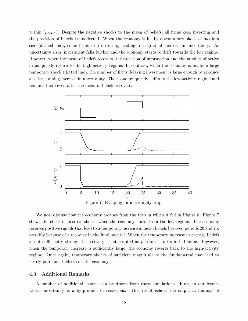
Figure 7: Escaping an uncertainty trap

We now discuss how the economy escapes from the trap in which it fell in Figure 6. Figure 7

shows the effect of positive shocks when the economy starts from the low regime. The economy

receives positive signals that lead to a temporary increase in mean beliefs between periods 20 and 25,

possibly because of a recovery in the fundamental. When the temporary increase in average beliefs

is not sufficiently strong, the recovery is interrupted as µ returns to its initial value. However,

when the temporary increase is sufficiently large, the economy reverts back to the high-activity

regime. Once again, temporary shocks of sufficient magnitude to the fundamental may lead to

nearly permanent effects on the economy.

4.3 Additional Remarks

A number of additional lessons can be drawn from these simulations. First, in our frame-

work, uncertainty is a by-product of recessions. This result echoes the empirical findings of

18

Bachmann et al. (2013) who show that uncertainty is partly caused by recessions and conclude,

by that, that it is of secondary importance for the business cycle. We show, however, that un-

certainty may still have a large impact on the economy by affecting the persistence and depth of

recessions, even if it is not what triggers them.

Second, as in models with learning in the spirit of Van Nieuwerburgh and Veldkamp (2006),

our theory provides an explanation for asymmetries in business cycles. In good times, since agents

receive a large flow of information, they react faster to shocks than in bad times.

Third, our economy may feature high uncertainty without volatility. For instance, in the low

regime, agents are highly uncertain about the fundamental but the volatility of economic aggregates

is low. Therefore, according to our theory, subjective uncertainty may affect economic fluctuations

even if no volatility is observed in the data. This distinguishes our approach from the existing

uncertainty-driven business cycle literature in the spirit of Bloom (2009). In particular, direct

measures of subjective uncertainty rather than measures of volatility are important to capture the

full amount of uncertainty in the economy.

Finally, a recent literature (Bachmann et al., 2013; Orlik and Veldkamp, 2013) uses survey data

to derive measures of uncertainty based on ex-ante forecast errors. Our model highlights a potential

shortcoming of this approach, as uncertainty about fundamentals differs from uncertainty about

endogenous variables, such as output or investment. For example, when the economy is trapped in

the low activity regime, firms know that all firms are uncertain, and therefore that investment is

likely to be low, such that the economy is less exposed to aggregate risk. As a result, their forecasts

about economic aggregates are accurate, even though their uncertainty about the fundamental is

high. As implied by the model, forecast errors about variables like output may not always be a

good proxy for uncertainty about fundamentals.

4.4 Policy Implications

The economy is subject to an information externality: in the decentralized equilibrium, firms

invest less often than they should because they do not internalize the release of information to

the rest of the economy caused by their investment. In Proposition 3, we solve the problem of a

constrained planner subject to the same information technology as individual agents. We show that

the decentralized economy is constrained inefficient, and that an investment subsidy is sufficient to

restore constrained efficiency.

Proposition 3. Under Assumptions 1-3, stated in the Appendix, the recursive competitive equilib-

rium is constrained inefficient. The efficient allocation can be implemented with positive investment

subsidies τ (µ, γ) and a uniform tax.

The subsidy that implements the optimal allocation takes a simple form to align social and

private incentives. As shown in the proof of the proposition, it is simply the sum of the social value

of releasing an additional signal to the economy and the private value of delaying investment.

19

The optimal policy being a subsidy, Proposition 3 implies that firms are more likely to invest in

the efficient allocation than in the laissez-faire economy. However, uncertainty traps can still arise

in the efficient allocation. Proposition 4 below establishes the result.

Proposition 4. Under Assumptions 1-2 and γx small enough, the planner’s allocation is subject

to an uncertainty trap for σf low enough and risk aversion “a” high enough.

The existence of uncertainty traps in the planner’s allocation may be surprising if one thinks

of the planner as a coordinator that should always prefer the high regime, as one might expect in

a model with multiple equilibria. As it turns out, transitioning from one regime to the other is

costly and risky. If the planner does not have more information than individual agents, it is still

optimal to wait when uncertainty is high enough. Hence, there may still exists a sufficiently strong

feedback from beliefs to actions in the constrained-efficient allocation to generate uncertainty traps.

However, while uncertainty traps remain present in the efficient allocation, they are less likely to

arise than in the laissez-faire economy because firms have stronger incentives to invest.

5 Quantitative Evaluation

To evaluate the quantitative importance of uncertainty traps, we now embed the mechanism

into a general equilibrium macroeconomic framework. We first describe the quantitative framework

and its parametrization. We then compare the model’s implications for standard business cycle

moments with the data and two alternative models: the RBC model and a restricted version of our

model in which uncertainty about the fundamental is fixed over time. Finally, we present our main

quantitative exercise, in which we compare the behavior of economic aggregates in the data against

the predictions from our model and alternative models in the context of the Great Recession.

5.1 Quantitative Model with Uncertainty Traps

We extend the baseline model along several dimensions. First, firms are now long-lived, use

both capital and labor to produce, and accumulate capital over time. They enter the economy

endogenously depending on economic conditions and exit exogenously. Second, firms are owned by

a risk-averse representative household that maximizes utility over consumption and leisure. Third,

factor and goods prices are endogenously determined in general equilibrium. As in the baseline

model, firms must pay an irreversible fixed cost to operate and social learning takes place when a

firm begins to produce. As a result, the number of entering firms responds to uncertainty about

the fundamental, and uncertainty depends on economic activity.

20

5.1.1 Preferences and Technology

The representative household chooses consumption Ct and labor Lt to maximize the expected

discounted sum of future utility

E

∞∑

t=0

βtU (Ct, Lt) , (12)

where 0 < β < 1 is the discount rate. The household supplies labor in a perfectly competitive

market at a wage wt. It also owns the firms in the form of claims to their dividends.

A single good used for consumption and investment is produced by a continuum of firms of

measure m. Each firm j ∈ [0,m] produces the final good by operating a Cobb-Douglas technology,

A (1 + θ)(

kαj l1−αj

)ω, 0 < α < 1, 0 < ω < 1,

using lj units of labor and kj units of capital. The parameter 0 < α < 1 controls the capital intensity.

The firm-level returns to scale, or span-of-control (Lucas Jr, 1978), parameter ω is assumed to be

strictly less than one to deliver a well-defined notion of firm size. The fundamental θ follows the

AR(1) process θ′ = ρθθ + εθ, with εθ ∼ iid N(

0,(

1− ρ2θ)

σ2θ)

.13 The total mass of firms m evolves

endogenously. Each period, a mass Q > 0 of potential entrants has the option to start production,

but only an (endogenous) fraction n of them does so. The mass Q remains fixed over time. Firms

exit at an exogenous rate δm > 0.

Each period, firms pay a fixed cost f common across firms and denominated in units of the

final good. We assume that f ∼ N(

µf , σ2f

)

is drawn independently over time.14 Due to the

irreversibilities created by these fixed costs, fewer firms enter in times of heightened uncertainty.

5.1.2 Information and Timing

As in the baseline model, agents do not observe the true value of the fundamental θ but learn

about it from two sources. First, they learn from a public signal Z. In contrast to the baseline model,

where this signal captured exogenous information released by media and statistical agencies, we now

explicitly model the signal Z as a summary of the information collected through the observation of

certain economic aggregates. As in any model with information frictions, restrictions about what

agents observe must be imposed to avoid perfectly revealing the fundamental. Agents cannot, for

instance, perfectly observe output as this would reveal θ. We assume instead that agents are able

to observe the value added of each firm, as well as its aggregate counterpart, but are unable to

perfectly distinguish between its individual components: revenue and fixed cost.15 As a result, a

13The additive specification of TFP, 1 + θ, ensures that the variance of beliefs about θ does not affect expectedoutput directly. As in our calibration the standard deviation of the ergodic distribution of θ is much smaller than 1,productivity is always positive in our simulations.

14The baseline theory included an idiosyncratic component to these fixed costs, which we ignore here for simplicity.Appendix E.4 performs sensitivity analysis on this assumption. We assume, however, that f is subject to aggregateshocks to be consistent with our information structure, as we explain in the next subsection.

15This assumption is in the spirit of Lucas (1972), where firms cannot distinguish between real and nominalshocks. A previous version of the paper assumed that firms cannot distinguish between aggregate and idiosyncratic

21

high level of value added may reflect either a high value of the fundamental θ or a low value of

the fixed costs.16 Second, and more specific to the channel we study in this paper, agents also

learn from signals emanating from others. As in the N → ∞ case of the baseline model, the entry

of an infinitesimal measure of firms dj releases a normally distributed signal xj about θ, observed

by everyone, with a precision γxdj, proportional to the mass of entrants. Again, the information

collected through this social learning channel can be summarized by a public signal X with precision

nQγx.17 All signals being public, beliefs are common across firms and the representative household.

In each period, events unfold as follows:

1. Incumbent firms, potential entrants and the household start with the same prior distribution

over the fundamental, θ | I ∼ N(

µ, γ−1)

. The fundamental θ and the fixed cost f are drawn

but unobserved.

2. The Q potential entrants decide whether to enter or not. A fraction n of them enters and

start producing next period.

3. The m incumbent firms choose labor and investment. The household decides how much labor

to supply and the labor market clears.

4. Fixed costs are paid, and production takes place. All agents observe the signal Z, which

captures the information contained in value added, and the signal X from new entrants, and

update their beliefs. A fraction δm of firms exogenously exits.

5.1.3 Firm-Level Problem

The aggregate state space of the economy is (µ, γ,K,m) where K =´m0 kjdj is the aggregate

capital stock. Realized individual profits for a firm operating with k units of capital and l units of

labor are18

π (k, l;µ, γ,K,m, θ, f) = A (1 + θ) kαωl(1−α)ω − w (µ, γ,K,m) l − f. (13)

The value of an incumbent firm that has accumulated k units of capital is then

V I (k;µ, γ,K,m) = maxk′,l

E

Uc (C,L)[

π (k, l;µ, γ,K,m, θ, f) + (1− δK) k − k′]

+ δmUc (C,L) k′ + β (1− δm)V

I(

k′;µ′, γ′,K ′,m′)

|µ, γ

, (14)

productivity shocks. The benefit of our current approach is to allow for a simple aggregation of the economy.16Despite this restriction on the observability of gross output and θ, all other economic aggregates are observed

and agents use all the available information to make their decision. However, as the timing will make clear, observingother variables such as the wage rate w, consumption C, the aggregate capital stock K, aggregate employment L,aggregate value added, the measure of entrants n, or the measure of incumbents m does not reveal any additionalinformation.

17A formal derivation of this information aggregation result is in Subsection 5.1.5.18Note that the presence of fixed operating costs could lead to negative profits. Since f is small relative to output

in our calibration, this virtually never happens.

22

subject to the laws of motion for the aggregate state variables µ, γ,K,m, described in the follow-

ing sections. The parameter 0 < δK < 1 is the depreciation rate of capital. This firm chooses labor

l and next-period capital k′ to maximize the expected sum of profits, discounted by the marginal

utility Uc (C,L), which plays the role of the stochastic discount factor. When a firm exits, which

happens with probability δm, its accumulated capital is scrapped and returned to the household at

the end of the period.

Consider now the problem of a potential entrant. In each period, a potential entrant decides

between waiting and entering. Its value is

V (µ, γ,K,m) = max

V W (µ, γ,K,m) , V E (µ, γ,K,m)

. (15)

If a potential entrant waits, it preserves the option of entering next period; hence the value of

waiting is

V W (µ, γ,K,m) = βE[

V(

µ′, γ′,K ′,m′)

|µ, γ]

. (16)

If, instead, the potential entrant decides to enter, its value is

V E (µ, γ,K,m) = maxk′e

(1− δm)E[

−Uc (C,L) k′e + βV I(

k′e;µ′, γ′,K ′,m′

)

|µ, γ]

. (17)

The definition of V E indicates that a potential entrant chooses the amount of capital k′e, carried

into the next period if it survives the δm shock or returned to the household at the end of the

period otherwise. Upon entry, its value next period is equal to the value of an incumbent firm that

has accumulated k′e units of capital, VI (k′e;µ

′, γ′,K ′,m′).

5.1.4 Aggregates

Incumbent and entrants face the same investment problem and choose the same next-period

capital level k′ (µ, γ,K,m). Therefore, next-period’s aggregate capital stock is

K ′ (µ, γ,K,m) = m′ (µ, γ,K,m) k′ (µ, γ,K,m) , (18)

where m′ (µ, γ,K,m) is the mass of incumbents next period, given by

m′ (µ, γ,K,m) = (1− δm) (m+ n (µ, γ,K,m)Q) . (19)

The fraction of entering firms among the Q potential entrants n (µ, γ,K,m) must be consistent

with individual entry decisions, in the sense that

n (µ, γ,K,m) =

1 if V E (µ, γ,K,m) > V W (µ, γ,K,m)

∈ [0, 1] if V E (µ, γ,K,m) = V W (µ, γ,K,m)

0 if V E (µ, γ,K,m) < V W (µ, γ,K,m) .

(20)

23

In turn, aggregate labor demand is

L (µ, γ,K,m) = m× l

(

K

m;µ, γ,K,m

)

, (21)

where l (k;µ, γ,K,m) is the firm-level labor demand resulting from (14).

5.1.5 Information and Beliefs

We now characterize the information contained in the signals observed by the agents. First, as

in the baseline model, the information diffused through social learning can be aggregated into a

single signal X which averages the individual signals released by entrants,19

X =1

nQ

ˆ nQ

0xjdj = θ + εX , εX ∼ N

(

0, (nQγx)−1)

, (22)

where nQγx, the endogenous precision of the social learning channel, changes with economic activ-

ity. Second, the information conveyed by observing value added is equivalent to the information

conveyed by the signal Z ∼ N(

θ, (γz (K,L,m))−1)

with precision20

γz (K,L,m) =

[

A

(

KαL(1−α)

m

)ω1

σf

]2

.

In contrast to the benchmark model, the precision γz of this signal now changes with economic

activity — a natural implication of assuming that agents observe economic aggregates instead of

the fundamental directly. In our calibrated economy, we find that fluctuations in γz, which depend

on the stock m of incumbent firms, are considerably smaller than fluctuations in the precision of

X, which depends on the flow n of incumbent firms. Therefore, the endogenous uncertainty in the

economy largely evolves as a function of the X signal.21

As in the baseline model, agents are fully rational and use all information available to update

their beliefs according to Bayes’ Law. The laws of motion for the mean and the precision of beliefs

19As in the infinite N case in the baseline model, X in expression (22) is to be understood as the distributional

limit of the average of N signals with precisions γx/N , i.e., lim 1N

∑N

1 xj ∼ N(

0,(

γxN/N)

−1)

as N → ∞ and

N/N → nQ.20Since all incumbent firms are identical, individual value added is A (1 + θ)

(

Km

)αω (

Lm

)(1−α)ω − f . Since K, L,

m and the distribution of f are known, observing value added is equivalent to observing θ− mω

AKαωL(1−α)ω (f − µf ) ∼

N(

θ,[

Am−ωKαωL(1−α)ω]

−2

σ2f

)

.

21In our calibrated economy, fluctuations in γz only accounts for 2.7% of the total fluctuation in uncertainty whilesocial learning through X accounts for the rest.

24

are

µ′ = ρθγµ + γzZ + nQγxX

γ + γz + nQγx, (23)

γ′ =

(

ρ2θγ + γz + nQγx

+(

1− ρ2θ)

σ2θ

)−1

. (24)

5.1.6 Recursive Competitive Equilibrium

We are now ready to define a competitive equilibrium for this economy.

Definition 3. A recursive competitive equilibrium is a collection of value functions V (µ, γ,K,m),

V W (µ, γ,K,m), V E (µ, γ,K,m) and V I (k;µ, γ,K,m) individual policy functions k′ (µ, γ,K,m),

k′e (µ, γ,K,m) and l (k;µ, γ,K,m), aggregate policy functions K ′ (µ, γ,K,m), m′ (µ, γ,K,m),

µ′ (µ, γ,K,m), γ′ (µ, γ,K,m), n (µ, γ,K,m), L (µ, γ,K,m) and C (µ, γ,K,m, θ, f), and wages

w (µ, γ,K,m) such that

1. The value functions V (µ, γ,K,m), V W (µ, γ,K,m), V E (µ, γ,K,m) and V I (k;µ, γ,K,m),

and the associated policy functions k′ (µ, γ,K,m), k′e (µ, γ,K,m) and l (k;µ, γ,K,m), solve

the Bellman equations (14)-(17) under the entry schedule n (µ, γ,K,m) and the laws of motion

K ′ (µ, γ,K,m),m′ (µ, γ,K,m), µ′ (µ, γ,K,m) and γ′ (µ, γ,K,m) given by (18), (19), (23) and

(24);

2. The fraction of entering firms n (µ, γ,K,m) satisfies the consistency equation (20);

3. The policy functions L (µ, γ,K,m) and C (µ, γ,K,m, θ, f) solve the household’s first order

condition on labor supply,

E [UL (C (µ, γ,K,m, θ, f) , L (µ, γ,K,m))]

E [UC (C (µ, γ,K,m, θ, f) , L (µ, γ,K,m))]= w (µ, γ,K,m) ;

4. The aggregate resource constraint is satisfied:

C (µ, γ,K,m, θ, f)+K ′ (µ, γ,K,m)−(1− δK)K+mf = A (1 + θ)m1−ω(

KαL (µ, γ,K,m)1−α)ω

.

5.2 Calibration

5.2.1 Standard Parameters

The time period is one quarter. Most of the moments that we target are computed starting

in 1978:Q1, when the Longitudinal Business Database (LBD) that we use for firm-level moments

begins, and stopping in 2007:Q3, at the onset of the 2007-2009 recession, allowing us to evaluate

the out-of-sample properties of the model in our Great Recession exercise. In our benchmark

specification, we assume GHH preferences, U = log(

C − L1+ν/ (1 + ν))

, and we also report the

results of our main quantitative exercise under CRRA preferences in Appendix C as robustness.22

22GHH preferences are common in the information frictions literature. We adopt them in our benchmark spec-ification because the usual CRRA preferences generate a counterfactual correlation between economic activity and

25

We set the Frisch elasticity ν = 2.84 which corresponds to the average aggregate Frisch elasticity

of hours reported by Chetty et al. (2011). The discount rate β is chosen to match an annual value

of 0.95. The depreciation rate is set to an annual value of 0.1.

For the production function parameters, we normalize A = 1 and set the returns-to-scale pa-

rameter ω to 0.89, which corresponds to the weighted average across 2-digit SIC estimates of the

returns to scale from Basu and Fernald (1997).23 We set the capital intensity parameter α so that

(1− α)ω = 0.645 to match the average labor compensation over GDP from 1978-2007 according

to annual data from the Penn World Table (Feenstra et al., 2015).24

We set δm = 2.6%, which corresponds to the employment-weighted firm exit rate for all firms

in the Longitudinal Business Database between 1978 and 2007. The mass of potential entrants Q

is normalized to 1.25

The parameters

ρθ, σ2θ

of the fundamental process θ are estimated using the quarterly

utilization-adjusted TFP series from Fernald (2014) over 1978Q1-2007Q3 after removing a linear

trend. This yields σθ = 0.028 and ρθ = 0.964.

5.2.2 Information and Fixed-Cost Distribution

With all the above parameters calibrated, it only remains to set values for the precision of

individual signals γx and the mean and variance of the distribution of fixed costs

µf , σ2f

. These

parameters govern the option-value effects and the evolution of Bayesian uncertainty about TFP.

To the best of our knowledge, no direct empirical measure exists for this concept of uncertainty.

The variance of beliefs about θ, however, is tightly related in our model to the ex-ante forecast

variance about endogenous variables like output. We thus target moments of the distribution of

uncertainty in output growth forecast provided by the Survey of Professional Forecasters (SPF)

and use this series as our main empirical proxy for uncertainty.

The SPF asks a panel of forecasters to provide the distribution of their beliefs about the growth

rate of real output in percentage terms between the current year and the last, and these distributions

are averaged across forecasters.26 We compute the standard deviation of this averaged distribution

in every year, and use moments of its time series to calibrate the model. To fit the parameters,

we compute the exact same object in a long-run simulation of our model. We pick the values

of γx, µf , σf by targeting the mean, the 5th percentile and the 95th percentile of the empirical

distribution of uncertainty over the 1992-2007 period, corresponding to the time period over which

positive signals (see Beaudry and Portier (2006) for a VAR estimation of the impact of news shocks). Upon receivinga positive signal about the economy, the wealth effect on the labor supply leads to a decline in output on impact.See Jaimovich and Rebelo (2009) for a discussion of the role of preferences in the news-shocks literature.

23Our parametrization corresponds to the γv parameter for the private economy estimated using OLS from Table2 in Basu and Fernald (1997).

24Specifically we use the series LABSHPUSA156NRUG from the FRED database.25For any given Q, we can replicate the aggregate allocation, albeit with a different measure of firms m, by rescaling

A, γx, µf and σf .26Specifically, at the beginning of each quarter, the SPF asks each forecaster to report the probability that growth

between the previous year and the current year will fall within each of several bins. We use forecast reported in the4th quarter, which represents a measure of uncertainty over just one quarter, because it maps easily into our model.

26

data on the distribution of real GDP growth is available in the SPF up to the beginning of the

Great Recession.

These three moments are directly informative about the three parameters that we need to

calibrate. The 95th percentile corresponds to periods of high uncertainty about real output growth,

which in the model correspond to periods with low firm entry when uncertainty is mostly driven

by the aggregate public signal Z, as opposed to the social learning signal X. Therefore, the

95th percentile is useful to identify σf which governs the informativeness of Z. Similarly, the 5th

percentile corresponds to periods of low uncertainty, which in the model correspond to periods of

high firm entry, when γx is the main driver of uncertainty. The average fixed cost µf affects the

average fraction of entrants n and relates to the average level of uncertainty.

The parameters are estimated by minimizing an equal-weighted distance between the empirical

and simulated moments. The numerical algorithm used to solve the model is described in Appendix

B. Table 1 reports the fit. The calibrated parameters are γx = 450, µf = 0.0115 and σf = 0.0155.

As the table shows, the calibrated model cannot match all moments at the same time. In particular,

because TFP is the only source of uncertainty while the SPF forecasters may worry about other

shocks, we have difficulty matching the upper tail of uncertainty in the data and there is on average

less uncertainty in our model. We thus view our results as conservative on the role of uncertainty

in the economy.

Uncertainty About GDP Growth Data (%) Model (%)

Mean 0.60 0.555th percentile 0.45 0.5095th percentile 0.73 0.64

Notes. Uncertainty is computed as the standard deviation of the SPF distribution over 1992Q4 to 2007Q4 of current year’sannual over last year’s annual real GDP stated in the last quarter of the current year. Growth rates and standard deviationsare stated in percentage terms. We use the 5% and 95% percentiles, instead of the min and the max, for robustness againstoutliers. Uncertainty in our model is computed over a simulation of 50,000 periods using the same definition as in the data.

Table 1: Calibrated Moments from the Survey of Professional Forecasters

5.3 Business-Cycle Moments

We now evaluate the performance of our model in explaining standard business cycle moments.

For that, we compare the benchmark model that we have just described against the data and

against two alternative models. The first alternative model (“RBC”) is the standard real business

cycle model under complete information, identically parametrized. The second model (“fixed θ-

uncertainty”) is a version of our model in which firms update their beliefs about the mean of the

fundamental θ (i.e., they update µ using (23)) but uncertainty (i.e., the inverse of the precision

of beliefs γ) remains constant at its long-run average in our benchmark model. Comparing our

full framework to the fixed θ-uncertainty model highlights the specific role played by endogenous

uncertainty.

Before comparing the models to the data, we must detrend the empirical time series. We note

that the cyclical properties we are interested in, in particular the persistence and depth of the Great

27

Recession, are sensitive to the specific detrending strategy. In Appendix A.2, we investigate the

implications of three filters: the Hodrick and Prescott (1997) (HP) filter, a linear detrending, and

a linear detrending allowing for a structural break in the trend. As shown in Figure 12a in that

appendix, the HP-filtered data suggests that the Great Recession was a mild economic downturn

and that the economy promptly recovered to its long-run trend after the trough. Both conclusions

contradict essential features of the raw output data shown in Figure 11a in Appendix A.2.27 We also

find that a purely linear trend exaggerates the severity and persistence of the recession by ignoring

low-frequency changes in the trend. Therefore, we choose a linear trend with a structural break

estimated by least squares (Hansen, 2000) as our benchmark, and we also report the sensitivity of

our results to using a standard linear trend.28 See Appendix A for a more detailed discussion of

the data and the detrending strategies.

We compute standard business cycle moments using the detrended data covering the period

between the first quarter of 1978 and the last quarter of 2014. For each of the three models,

we generate ten thousand simulations of the same length as the data (148 quarters), and then

average each moment across all simulations. Panel A of Table 2 reports the results for the standard

deviation of output (Y ), consumption (C), employment (L), investment (I), the number of firms

(m) and uncertainty about real output growth (U). Panel B reports the correlation between each

of these variables and output, and Panel C reports their autocorrelation.

Because of the absence of learning, the RBC model generates more volatility in every variable

than our full model. However, their performances are overall similar. Regarding the volatility

of uncertainty about real output growth, our model is able to explain only a fraction of what is

observed in the data, suggesting that other shocks — possibly exogenous uncertainty shocks —

may be needed to fully account for the total fluctuations in uncertainty. Note that uncertainty

about current-quarter real output growth is 0 in the RBC model under full information. Panels B

and C show that the benchmark, the fixed θ-uncertainty model and the RBC model are roughly

comparable in terms of the correlations with output and the autocorrelations.

27See King and Rebelo (1993) and Cogley and Nason (1995a) for a discussion of various drawbacks of the HPfilter.

28An additional advantage of the linear trends is that they allow us to cleanly interpret the (unfiltered) predictionof forecasters reported in the SPF data used to calibrate the model. For instance, a 2% growth forecast for this yearrelative to the previous year can be directly mapped to the model by removing the long-run growth rate in outputfrom the linear filter. It is unclear how the analog exercise would be done if the data is HP filtered and detrendedwith a bandpass filter. See Appendix A.2 for a detailed discussion of the filters.

28

Y C L I m U

A. Standard DeviationData 0.039 0.031 0.066 0.132 0.038 0.253Benchmark 0.035 0.030 0.027 0.072 0.020 0.053Fixed θ-uncertainty 0.036 0.031 0.027 0.076 0.019 0.027RBC 0.044 0.036 0.033 0.093 – –

B. Correlation w.r.t YData 1 0.588 0.921 0.523 0.646 -0.443Benchmark 1 0.967 0.884 0.855 0.459 -0.644Fixed θ-uncertainty 1 0.966 0.888 0.858 0.480 -0.619RBC 1 0.987 1 0.944 – –

C. Autocorrelation (1st lag)Data 0.981 0.982 0.993 0.962 0.995 0.762Benchmark 0.956 0.943 0.942 0.918 0.991 0.931Fixed θ-uncertainty 0.957 0.943 0.941 0.915 0.989 0.869RBC 0.934 0.949 0.934 0.907 – –

Notes. All series are computed in log deviation from trend. Each of the 10,000 replications of the simulated series are linearly

detrended. The annual series for m is interpolated to quarterly data. Uncertainty U is the standard deviation of current year

real output growth expressed in the last quarter of the current year. Because it is only available annually and, by definition,

cannot simply be interpolated, the moments we report about uncertainty are computed using observations from the 4th quarter

of every year. Its annual autocorrelation is expressed in quarterly terms. C is gross of fixed costs for comparison across models.

Employment and output are perfectly correlated in the RBC model as a consequence of the GHH preferences.

Table 2: Business-Cycle Moments: Data, RBC, and Benchmark Model

The key conclusion from Table 2 is that a standard calibration of our model performs similarly to

the RBC model in terms of standard business-cycle moments. Therefore, incorporating endogenous

uncertainty in a standard business cycle model does not impair its ability to predict well-known

patterns of business cycle data. This result should not be surprising. As we saw in the baseline

model, the uncertainty trap mechanism kicks in only for large shocks, which are rare in these

simulations. In the next section, we show that the key difference between our model and standard

models, and the value added of modeling uncertainty traps, lies in terms of predicting how the

economy responds to large shocks.

5.4 Policy Function and Impulse Responses

We now examine the role of endogenous uncertainty in propagating shocks. First, we ask

whether the key implication of the uncertainty trap mechanism identified in the baseline theory

— generating protracted recessions out of sufficiently negative shocks — is also at work in the full

calibrated model. In the next section, we ask whether this feature of the model can help explain

the behavior of macro aggregates during the Great Recession.

Firm Entry and Beliefs In Proposition 1 we showed that, under certain conditions, the mass

of producing firms increases with the mean of beliefs µ and decreases with uncertainty (increases

29

with γ). We verify that these properties are inherited by the calibrated quantitative model. Figure

8 plots the fraction of entering firms n (µ, γ,K,m) as a function of mean beliefs µ, for three levels of

uncertainty. Similarly to Figure 4 in the baseline theory, we find that, for any level of uncertainty,

firms are more likely to enter when beliefs are more optimistic and that, for any level of mean

beliefs, firms are more likely to enter when uncertainty is lower. Therefore, the entry decision of

the quantitative model inherits the key feature of the baseline theory leading to uncertainty traps.

-0.06 -0.04 -0.02 0

Mean of beliefs

0

0.5

1

Mas

s en

teri

ng

firm

s

High uncertainty

Medium uncertainty

Low uncertainty

Notes. This figure was generated with K and m at their steady-state values when shocks are set to zero.

Figure 8: Investment decision n(µ, γ,K,Q) for K and m constant at their steady-state level.

Response to Small and Large Shocks A central feature of uncertainty traps is the non-linear

response to shocks, shown in Figure 6 in the context of the baseline theory. For shocks leading

to large negative drops in the mean of beliefs, endogenous uncertainty leads to recessions which

are relatively deeper and last relatively longer than for small shocks. We ask whether the full

quantitative model inherits this feature. Figure 9 shows the evolution of the mean of beliefs µ, the

precision of beliefs γ, and output Y after a one-period drop in mean beliefs of 1% (left column)

and 5% (right column) in both the full model and the fixed θ-uncertainty model.29 In the fixed-

information model, the economy starts to recover immediately after the initial shock regardless of

the size of the shock. In contrast, in the full model, output continues to decline after the mean

of beliefs has started to recover. Moreover, the duration of this decline is longer the larger is the

shock. Reaching the trough in output takes 6 quarters in response to the small shock, and 15

quarters in response to the larger one. As in the baseline model, this non-linearity is driven by the

endogenous evolution of uncertainty. The fall in mean beliefs drives down the incentives to enter.

As a result, fewer signals are released and the precision of beliefs falls (panels (c) and (d)). After

the shock, agents receive signals suggesting an improvement in the fundamental, and beliefs recover

(panels (a) and (b)). However, the recovery in output is delayed in the full model by the feedback

between high uncertainty (panels (e) and (f)) and slow entry.

29Fundamental shocks affect the policy functions only through beliefs. Falls in beliefs may result from shocks tothe fundamental θ or to the signals, X and Z.

30

(a) Small shock - mean beliefs µ

0 10 20 30 40 50 60

Lags

-0.01

0

Fixed uncertainty

Full model

(b) Large shock - mean beliefs µ

0 10 20 30 40 50 60

Lags

-0.05

0

(c) Small shock - precision of beliefs γ

0 10 20 30 40 50 60

Lags

2000

3000

(d) Large shock - precision of beliefs γ

0 10 20 30 40 50 60

Lags

2000

3000

(e) Small shock - output Y

0 10 20 30 40 50 60

Lags

-0.015

-0.01

-0.005

0

(f) Large shock - output Y

0 10 20 30 40 50 60

Lags

-0.05

-0.025

0

Notes: The left column shows the response of the economy to a -1% one-period shock to µ. The right column shows theresponse of the economy to a -5% one-period shock to µ. The solid curves show the evolution of the economy according to thefull model, while the dashed curves show the evolution of a control economy in which the flow of public information is fixed atthe steady-state level of the full model. Figures (e) and (f) are in log deviation from trend, the other figures are in level.

Figure 9: Mean beliefs, precision of beliefs and output in response to a one-period shock

Table 3 summarizes the properties of the recessions depicted in Figure 9. For both shocks, the

table reports the ensuing recession’s depth (the magnitude of the peak-to-trough fall in output) and

the half-life of the recovery (the number of quarters for the economy to recover half of the peak-to-

trough fall in output). The table highlights two key features of uncertainty traps: i) endogenous

uncertainty makes recessions deeper and longer for shocks of any magnitude (recessions’ depth and

duration are larger in the full than in the fixed θ-uncertainty model), and ii) the differential effect

of endogenous uncertainty is relatively larger for large than for small shocks. The recession is 22%

deeper and 40% longer in the full model than in the fixed θ-uncertainty model under a negative 1%

shock to beliefs, but 35% deeper and 66% longer under a negative 5% shock. Therefore, in the full

calibrated model, endogenous uncertainty leads to amplification and persistence of shocks driving

down beliefs.

Small shock (-1%) Large shock (-5%)

Depth 50% recovery Depth 50% recoveryFull model -1.1% 42 -6.2% 58Fixed θ-uncertainty -0.9% 30 -4.6% 35

Notes. The depth of the recession corresponds to the lowest value of output reached since the official beginning of the recession.The “50% recovery” column is the number of quarters before the economy recovers 50% of the peak-to-trough drop in output.

Table 3: The impact of shock sizes on the depth and duration of recessions across models

31

5.5 Endogenous Uncertainty in U.S. Recessions

Our previous discussion established that, within our calibrated model, endogenous uncertainty

amplifies and lengthens the decline in economic activity relatively more for large than for small

shocks. We now evaluate the role of endogenous uncertainty in explaining the U.S. experience

during past recessions. Specifically, we ask whether it can help explain the observed depth and

persistence of a recession when there is a large enough shock and if, indeed, the mechanism only

“kicks in” for sufficiently large shocks.

To implement this exercise we must first take a stand on the exogenous shocks that hit the

U.S. economy in each recession. Within our model, the only exogenous shocks are the innovations

to the signals Xt, Zt and to the fundamentals θt. The shocks to fundamental θt are taken

directly from the data. To discipline the evolution of Xt, Zt, we choose their innovations such

that our model and the fixed θ-uncertainty model exactly reproduce, as equilibrium outcomes, the

forecast of current year’s real output from the SPF during the first part of each recession.30 We

then compute the response of the three models we have introduced – our full quantitative model,

the fixed θ-uncertainty model, and the RBC model – and contrast them with the data. Importantly,

among the variables that we simulate and contrast against the data we include uncertainty about

output growth from the SPF and the number of firms, both of which are directly related to the

forces in the model.

We implement this exercise in the context of the largest and second-largest recessions in terms

of decline in output within our sample, the Great Recession and the 1981-1982 recession. Since we

expect uncertainty traps to be more important after large shocks, the Great Recession — the most

important downturn since the Great Depression — is a historical episode where we would expect

endogenous uncertainty to play a role. However, we also verify that endogenous uncertainty does

not transform every downturn into a deeply protracted recession. For that, we also consider the

impact of the mechanism during the 1981-1982 recession, which was characterized by a large but

brief decline in productivity and was followed by a relatively rapid recovery in output. We expect

the impact of endogenous uncertainty to be relatively weaker during this episode.

5.5.1 Great Recession

We start by considering the Great Recession. According to the NBER, the recession took place

over the period 2007:Q4-2009:Q2. We first feed the model with the observed TFP shocks over

the corresponding period.31 We then feed each model with a series of signals that allows them to

30Note that we do not need to specify exactly the combination of Xt and Zt shocks that is needed to match outputforecasts. Only the time series of µt is relevant for our purpose. In the case of the RBC model we only introduceshocks to θt, as there is no degree of freedom to match the forecast about real output.

31We pick 2007:Q2 as our start date to be consistent with the dates at which we match output forecasts. However,we stop feeding the series in 2008:Q4 because the TFP series from Fernald (2014) displays a large increase at thebeginning of 2009, which leads to a strong counterfactual expansion in the RBC economy (the other models farebetter). For robustness, we fit the full TFP series in Figure 13 of Appendix C and experiment with other TFP seriesin Figures 15 and 16. In all cases, the full model generates a deeper and longer recession than the fixed θ-uncertaintyand RBC models.

32

replicate output forecasts from the SPF over that period. Specifically, the SPF surveys forecasters

every quarter about their point expectations for the level of real output for the current year. Since

the trough in output forecast from the SPF was reached in 2009:Q2, we focus on second quarter

forecasts and match expectations about current year output in 2007:Q2, 2008:Q2, and 2009:Q2.32

Figure 10 shows the evolution of TFP, real output forecasts, output, investment, employment,

consumption, the number of firms, and uncertainty about real GDP growth. The solid lines in the

left column represent the data. The right column shows the predictions of the three models: the full

quantitative model (solid blue curves), the fixed θ-uncertainty model (dashed brown curves), and

the RBC model (dot-dash pink curves). The diamonds in panel (b) and (d) of Figure 10 indicate

the data that the models are calibrated to match. All shocks and innovations are set to zero after

2009:Q2, and the economy is left to recover.

The central finding of this exercise, is that for all macro aggregates that we consider (output,

investment, consumption, employment, number of firms and uncertainty about GDP growth), our

model generates dynamics which are closer to the data than the fixed θ-uncertainty model and the

RBC model. Panel (f) of Figure 10 shows that the decline in output is clearly deeper and more

protracted in our model than in the alternative models.

Table 4 summarizes the key properties of the recession in the data and as predicted by the three

models. The first column shows the depth of the recession, measured as the percentage drop in

output from the beginning of the recession to its lowest value. The full model is able to explain

almost all of the depth, while the fixed θ-uncertainty model and the RBC model account for 76%

and 33% of the fall, respectively. The second column of the table shows the earliest date at which

output has recovered 20% of the depth.33 In the full model, output recovers 20% of the lost ground

in 2015:Q1, close to corresponding date in the data (2014:Q3). In contrast, in the fixed θ-uncertainty

and in the RBC models this event happens in 2012:Q4 and 2009:Q3, respectively. These results

imply that, within our model, endogenous uncertainty adds 1.8 (5.2) percentage points in terms of

depth and about two (five) years until the 20% recovery relative to the fixed θ-uncertainty (RBC)

model. Finally, the third column shows the cumulative loss in output, measured as the sum of the

percentage deviations from trend from 2007:Q4 to 2015:Q1, the end of our sample. This measure

combines the depth and the persistence of the recession into a single statistic. If we normalize

this measure by the output produced in quarter 2007:Q4 at the onset of the recession, the U.S.

economy lost a cumulated 1.84 quarters of output since that date. Our full model explains 93% of

this loss, while the fixed θ-uncertainty and RBC models can account for 73% and 30% of the loss,

32Forecasts in the first, third or fourth quarters in the SPF are about the current year and thus correspond toforecasts at different horizons. We focus on a single horizon with second-quarter forecasts to avoid using four differentdefinitions of forecast in our model. Since we do not use forecast data in Q1, Q3 and Q4, we linearly interpolatethe series of µt at these points. Note finally that the empirical output forecast series stops in 2009:Q2 because of achange in variable definition.

33We cannot use the standard half-life measure of persistence since output has not recovered half of the way fromits trough in the data. We pick the 20% threshold as it roughly corresponds to the level attained by output in thedata at the end of the sample. The full model also generates a longer recession measured in terms of the number ofquarters from peak to trough relative to alternative models. The exact date for the trough is however hard to identifyin the data because of high-frequency noise.

33

respectively. According to these various measures, our full model is better able to account for the

overall severity of the recession.

Depth 20% recovery Cumulative loss

Data -7.9% 2014:Q3 -184%Full model -7.8% 2015:Q1 -171%Fixed θ-uncertainty -6.0% 2012:Q4 -134%RBC -2.6% 2009:Q3 -56%

Notes. We compute the depth, persistence, and cumulative loss of the recession from the official beginning of the recession in2007:Q4 as determined by the NBER. The depth of the recession corresponds to the lowest value of output reached since theofficial beginning of the recession. The “20% recovery” column is the earliest date at which output recovers 20% of the depth.Cumulative loss is the sum of the percentage deviation of output from trend from 2007:Q4 to 2015:Q1.

Table 4: Depth, persistence, and cumulative output loss of the Great Recession

Besides output, endogenous uncertainty can also help explain the behavior of other aggregates.

As shown in panels (g) and (h), even though our model does not generate as pronounced a decline

in investment, it does generate more persistence than the alternative models. Panels (m) and (n)

of Figure 10 show that the number of firms also falls. By construction, the RBC model does not

have predictions in this regard. Our full quantitative model does well in predicting the persistence

and the amplitude of the fall in the number of active firms. Since entry and the number of firms

govern the dynamics of uncertainty within the full model, the good performance of the model along

that dimension is reassuring. Our model generates as large a fall in consumption as it is observed

in the data (panels (k) and (l)). Relative to the alternative models, it also predicts a larger fall

and a more protracted recovery in employment (panels (i) and (j)), better reflecting the empirical

patterns. Even though for most variables the fall in economic aggregates happens faster in the

data, our model is closer to the empirical series than the alternative models for all the variables

reported in the figure.

We also highlight that our model is relatively successful at explaining the shape of the uncer-

tainty response. As observed in panels (o) and (p) of Figure 10, the uncertainty in output growth

follows an inverted-U shape relationship that our model reproduces, although in our model the

peak in uncertainty is delayed relative to the data. In contrast, the alternative models generate

little variation in uncertainty in GDP forecasts.

Sensitivity

We demonstrate the robustness of our findings by replicating the Great Recession exercise under

alternative assumptions: i) fitting the whole TFP series instead of only its beginning; ii) using a

simple linear detrending instead of allowing for a structural break; iii) using TFP data from the Penn

World Table and the Bureau of Labor Statistics instead of the Fernald time series; and iv) using

34

(a) TFP (data)

2007 2008 2009 2010 2011 2012 2013 2014 2015

-0.05

0

(b) TFP (models)

2007 2008 2009 2010 2011 2012 2013 2014 2015

-0.05

0

(c) Forecast Y (data)

2007 2008 2009 2010 2011 2012 2013 2014 2015

-0.1

-0.05

0

(d) Forecast Y (models)

2007 2008 2009 2010 2011 2012 2013 2014 2015

-0.1

-0.05

0

(e) Output Y (data)

2007 2008 2009 2010 2011 2012 2013 2014 2015

-0.05

0

(f) Output Y (models)

2007 2008 2009 2010 2011 2012 2013 2014 2015

-0.05

0

(g) Investment I (data)

2007 2008 2009 2010 2011 2012 2013 2014 2015

-0.4

-0.2

0

(h) Investment I (models)

2007 2008 2009 2010 2011 2012 2013 2014 2015

-0.4

-0.2

0

(i) Labor L (data)

2007 2008 2009 2010 2011 2012 2013 2014 2015

-0.1

0

(j) Labor L (models)

2007 2008 2009 2010 2011 2012 2013 2014 2015

-0.1

0

(k) Consumption C (data)

2007 2008 2009 2010 2011 2012 2013 2014 2015

-0.05

0

(l) Consumption C (models)

2007 2008 2009 2010 2011 2012 2013 2014 2015

-0.05

0

(m) Mass of firms m (data)

2007 2008 2009 2010 2011 2012 2013 2014 2015

-0.1

0

(n) Mass of firms m (models)

2007 2008 2009 2010 2011 2012 2013 2014 2015

-0.1

0

(o) Uncertainty about growth (data)

2007 2008 2009 2010 2011 2012 2013 2014 2015

0

0.2

0.4

(p) Uncertainty about growth (models)

2007 2008 2009 2010 2011 2012 2013 2014 2015

0

0.2

0.4

Notes. The left column shows the data while the right column shows the models. In the right column, the solid curves show

the full model, the dashed brown curves show fixed θ-uncertainty model and the dot-dash pink curves show the RBC model.

All figures are in log deviation from trend. The scales are the same in both columns.

Figure 10: Great Recession - Data and models

35

standard CRRA preferences instead of the GHH preferences assumed in the main exercise. The full

simulations from these robustness exercises are included in Appendix C. Table 5 summarizes these

simulations by showing the cumulative loss in output generated by each model in each exercise,

and comparing it to the data. In all cases, we find that our conclusions are robust. The full model

with endogenous uncertainty gets closer to the data by generating more severe recessions than the

alternative models. Table 7 in the Appendix shows that the full model generates deeper and longer

lasting recessions in all the robustness exercises.

Cumulative loss in output

Data Full model Fixed θ-uncertainty RBC

Benchmark -184% -166% -129% -56%Full TFP fit -184% -86% -38% +38%Linear detrending -310% -173% -139% -72%PWT TFP -184% -194% -175% -131%BLS TFP -184% -171% -142% -85%CRRA Preferences -184% -80% -65% -31%

Notes. Cumulative loss is the sum of the percentage deviation of output from trend from 2007:Q4 to 2015:Q1.

Table 5: Robustness: Cumulative loss during the Great Recession

5.5.2 1981-1982 Recession

We now consider the impact of endogenous uncertainty in the less severe recession of 1981Q3-

1982Q4. The purpose of this section is to show that, while endogenous uncertainty generates

amplification and persistence in response to very large shocks, it does not necessarily increase the

depth and persistence of every negative shock. As such, the model does not have counterfactual

implications for the magnitude and persistence of milder recessions.

Table 6 replicates Table 4 for the 1981-1982 recession.34 We see that the full and the fixed θ-

uncertainty models generate shallower recessions than the data, while output drops more than the

data in the RBC model. In terms of persistence, the three models performs similarly, suggesting

that the economy should have recovered 20% of the loss in output at the beginning of 1984 —

about a year after that threshold was reached in the data. In terms of cumulative loss, all models

predict recessions that are more severe than the data, although the difference between model and

data is larger for the RBC than for the full and fixed θ-uncertainty models. Overall, we find that

for the 1981-1982 recession, characterized by a less severe combination of TFP and beliefs shocks,

endogenous uncertainty does not generate additional persistence. This confirms that the full model

generally behaves as a standard RBC model, except during large unusual downturns, such as the

2007-2009 recession, when the uncertainty trap mechanism kicks in.

34Since the output forecast series is fully available over the period 1981-1985, we fit the whole time series of bothbeliefs and TFP. Appendix D shows the model predicted series.

36

Depth 20% recovery Cumulative loss

Data -5.3% 1983:Q2 -13%Full model -4.9% 1984:Q1 -32%Fixed θ-uncertainty -4.7% 1984:Q1 -32%RBC -6.4% 1984:Q2 -44%

Notes. The table is constructed similarly to Table 4. The official beginning of the recession is in 1981:Q3, and the cumulativeloss is computed between that quarter and 1985:Q1.

Table 6: Depth, persistence and cumulative output loss of the 1981-1982 recession

5.6 Further Applications

In Appendix E we provide additional exercises that highlight various features of the model.

First, we show that, like other studies of the effects of uncertainty on the economy (Bloom, 2009;

Bloom et al., 2012), exogenous uncertainty shocks generate recessions in our framework. In our

model, these exogenous shocks are propagated endogenously through the endogenous uncertainty

channel.

Second, we consider the problem of a social planner in Appendix E.2. To do so, we compute the

efficient allocation and consider how it responds to shocks relative to the competitive equilibrium

that we have studied so far. We find that the planner prevents the number of entering firms from

falling too much during the recession in order to prevent uncertainty from rising too much. As a

result, the recession is shorter and shallower in the planner’s allocation, suggesting a potential role

for government policies in mitigating the impact of recessions.

Third, we show in Appendix E.3 that our benchmark model improves on RBC in terms of

propagation of shocks. As noted by Cogley and Nason (1995b), the RBC model features weak

internal persistence so that the properties of GDP growth mimic those of the exogenous TFP

growth process. In our full model, however, the persistence in output growth is larger than in TFP

growth, and more so at lower lags. Hence, while our model does not replicate the full amount of

autocorrelation observed in the data, it does reproduce the qualitative feature of the data that the

autocorrelation of GDP growth is larger than that of TFP growth at lower lags. We interpret this

finding as evidence that endogenous uncertainty leads to a more persistent series for output growth

relative to TFP growth, in line with the baseline theory.

6 Conclusion

We develop a theory of endogenous uncertainty and business cycles that combines two forces:

higher uncertainty about economic fundamentals deters investment, and uncertainty evolves en-

dogenously because agents learn from the actions of others. The interaction between investment

and uncertainty leads to uncertainty traps: episodes in which high uncertainty leads firms to delay

investment, further raising uncertainty. In the unique equilibrium of the model, the economy fluc-

37

tuates between a high-activity/low-uncertainty regime and a low-activity/high-uncertainty regime

and is subject to strong non-linear dynamics in which large shocks can have near permanent effects.

To quantify the importance of uncertainty traps, we embed the mechanism in a business cycle

model. We calibrate the model to the United States economy and find that endogenous uncertainty

increases the depth and duration of recessions, particularly after large shocks. We also find that

our full model is able to better explain the behavior of standard macro aggregates during the Great

Recession than alternative models.

We believe that the novel channel proposed in this paper is important for several reasons.

First, the emphasis on subjective uncertainty — and beliefs about fundamentals in particular —

implies that not only exogenous volatility shocks, but also other sources of uncertainty, matter for

the economy. Thus, we view recent empirical work using survey data on forecasts or consumer

and business expectations as an important step towards a more complete understanding of the

role of uncertainty in business cycles. Second, we believe that our framework may be useful as

a theoretical benchmark for empirical and quantitative studies seeking to estimate the direct and

feedback effects of uncertainty on economic activity. Despite the multiplicity of regimes and strong

non-linearities, the model features a single competitive equilibrium, which makes it amenable to

applied work. Third, we have shown that allowing uncertainty to fluctuate endogenously leads

to a significant propagation and amplification mechanism. The type of non-linearities and the

multiplicity in regimes that we obtain may be of broader interest for business cycle modeling in

general and could also shed light on some particularly large historical downturns.

For the sake of clarity, we have exposited the mechanism in a purposely simple framework, but

a number of generalizations may be worth investigating. In particular, it would be interesting to

understand how uncertainty traps interact with frictions that could magnify their impact, such as

financial frictions, demand externalities, or belief heterogeneity. We leave these questions to future

research.

38

References

Amador, M. and P.-O. Weill (2010): “Learning from Prices: Public Communication and

Welfare,” Journal of Political Economy, 118.

Angeletos, G.-M., C. Hellwig, and A. Pavan (2007): “Dynamic global games of regime

change: Learning, multiplicity, and the timing of attacks,” Econometrica, 75, 711–756.

Arellano, C., Y. Bai, and P. Kehoe (2012): “Financial Markets and Fluctuations in Un-

certainty,” Working paper, Federal Reserve Bank of Minneapolis and NBER; Arizona State

University; University of Minnesota and Federal Reserve Bank of Minneapolis.

Bachmann, R. and C. Bayer (2013): “Wait-and-See Business Cycles?” Journal of Monetary

Economics, 60, 704–719.

——— (2014): “Investment Dispersion and the Business Cycle,” The American Economic Review,

104, pp. 1392–1416.

Bachmann, R., S. Elstner, and E. R. Sims (2013): “Uncertainty and Economic Activity:

Evidence from Business Survey Data,” American Economic Journal: Macroeconomics, 5, 217–

49.

Bachmann, R. and G. Moscarini (2011): “Business cycles and endogenous uncertainty,”

manuscript, Yale University, July.

Banerjee, A. V. (1992): “A simple model of herd behavior,” The Quarterly Journal of Economics,

107, 797–817.

Barro, R. J. (2006): “Rare disasters and asset markets in the twentieth century,” The Quarterly

Journal of Economics, 823–866.

Barro, R. J. and J. F. Ursua (2012): “Rare Macroeconomic Disasters,” Annual Review of

Economics, 4, 83–109.

Basu, S. and J. G. Fernald (1997): “Returns to scale in US production: Estimates and impli-

cations,” Journal of political economy, 105, 249–283.

Beaudry, P. and F. Portier (2006): “Stock Prices, News, and Economic Fluctuations,” The

American Economic Review, 96, 1293–1307.

Benhabib, J., P. Wang, and Y. Wen (2015): “Sentiments and Aggregate Demand Fluctua-

tions,” Econometrica, 83, 549–585.

Bikhchandani, S., D. Hirshleifer, and I. Welch (1992): “A theory of fads, fashion, custom,

and cultural change as informational cascades,” Journal of political Economy, 992–1026.

39

——— (1998): “Learning from the Behavior of Others: Conformity, Fads, and Informational Cas-

cades,” The Journal of Economic Perspectives, 12, pp. 151–170.

Bloom, N. (2009): “The Impact of Uncertainty Shocks,” Econometrica, 77, 623–685.

Bloom, N., M. Floetotto, N. Jaimovich, I. Saporta-Eksten, and S. Terry (2012): “Re-

ally Uncertain Business Cycles,” Nber working paper no.18245, NBER.

Canova, F. (1998): “Detrending and business cycle facts,” Journal of Monetary Economics, 41,

475 – 512.

Caplin, A. and J. Leahy (1993): “Sectoral shocks, learning, and aggregate fluctuations,” The

Review of Economic Studies, 60, 777–794.

Carlsson, M. (2007): “Investment and Uncertainty: A Theory-based Empirical Approach,” Ox-

ford Bulletin of Economics and Statistics, 69, 603–617.

Chamley, C. (1999): “Coordinating regime switches,” The Quarterly Journal of Economics, 114,

869–905.

——— (2004): “Delays and equilibria with large and small information in social learning,” European

Economic Review, 48, 477 – 501.

Chamley, C. and D. Gale (1994): “Information revelation and strategic delay in a model of

investment,” Econometrica: Journal of the Econometric Society, 1065–1085.

Chetty, R., A. Guren, D. Manoli, and A. Weber (2011): “Are micro and macro labor

supply elasticities consistent? A review of evidence on the intensive and extensive margins,” The

American Economic Review, 101, 471–475.

Cogley, T. and J. M. Nason (1995a): “Effects of the Hodrick-Prescott filter on trend and

difference stationary time series Implications for business cycle research,” Journal of Economic

Dynamics and control, 19, 253–278.

——— (1995b): “Output Dynamics in Real-Business-Cycle Models,” The American Economic

Review, 85, pp. 492–511.

Decker, R. A. and P. N. D’Erasmo (2016): “Market exposure and endogenous firm volatility

over the business cycle,” American Economic Journal: Macroeconomics, 8, 148–198.

Dixit, A. K. and R. S. Pindyck (1994): Investment under uncertainty, Princeton university

press.

Dontchev, A. L. and R. T. Rockafellar (2009): “Implicit functions and solution mappings,”

Springer Monographs in Mathematics. Springer, 194.

40

Farmer, R. (2013): “Animal Spirits, Financial Crises and Persistent Unemployment,” Economic

Journal, 123, 317–340.

Feenstra, R. C., R. Inklaar, and M. P. Timmer (2015): “The Next Generation of the Penn

World Table,” American Economic Review, 105, 3150–3182.

Fernald, J. G. (2014): “A Quarterly, Utilization-Adjusted Series on Total Factor Productivity,”

Manuscript, Federal Reserve Bank of San Francisco.

Foster, A. D. and M. R. Rosenzweig (1995): “Learning by Doing and Learning from Others:

Human Capital and Technical Change in Agriculture,” Journal of Political Economy, 103, pp.

1176–1209.

Gabaix, X. (2012): “Variable Rare Disasters: An Exactly Solved Framework for Ten Puzzles in

Macro-Finance*,” The Quarterly journal of economics, 127, 645–700.

Gilchrist, S., J. W. Sim, and E. Zakrajsek (2014): “Uncertainty, financial frictions, and

investment dynamics,” Tech. rep., National Bureau of Economic Research.

Gourio, F. (2012): “Disaster Risk and Business Cycles,” American Economic Review, 102, 2734–

66.

Guiso, L. and F. Schivardi (2007): “Spillovers in Industrial Districts,” The Economic Journal,

117, pp. 68–93.

Hansen, B. E. (2000): “Testing for structural change in conditional models,” Journal of Econo-

metrics, 97, 93–115.

Hodrick, R. J. and E. C. Prescott (1997): “Postwar U.S. Business Cycles: An Empirical

Investigation,” Journal of Money, Credit and Banking, 29, 1–16.

Jaimovich, N. and S. Rebelo (2009): “Can News about the Future Drive the Business Cycle?”

American Economic Review, 99, 1097–1118.

Jurado, K., S. C. Ludvigson, and S. Ng (2015): “Measuring uncertainty,” American Econon-

mic Review, 105, 1177–1216.

Kaplan, G. and G. Menzio (2013): “Shopping Externalities and Self-Fulfilling Unemployment

Fluctuations,” .

Kehrig, M. (2011): “The cyclicality of productivity dispersion,” US Census Bureau Center for

Economic Studies Paper No. CES-WP-11-15.

Kim, T. (1993): “Differentiability of the Value Function,” .

King, R. G. and S. T. Rebelo (1993): “Low frequency filtering and real business cycles,”

Journal of Economic Dynamics and Control, 17, 207 – 231.

41

Kozlowski, J., L. Veldkamp, and V. Venkateswaran (2015): “The Tail that Wags the

Economy: Belief-Driven Business Cycles and Persistent Stagnation,” Working paper.

Lang, W. W. and L. I. Nakamura (1990): “The dynamics of credit markets in a model with

learning,” Journal of Monetary Economics, 26, 305 – 318.

Lucas, R. E. (1972): “Expectations and the neutrality of money,” Journal of Economic Theory,

4, 103 – 124.

Lucas Jr, R. E. (1978): “On the size distribution of business firms,” The Bell Journal of Eco-

nomics, 508–523.

Morris, S. and H. S. Shin (1998): “Unique equilibrium in a model of self-fulfilling currency

attacks,” American Economic Review, 587–597.

——— (1999): “A theory of the onset of currency attacks,” The Asian Financial Crisis, 230.

Ordonez, G. L. (2009): “Larger crises, slower recoveries: the asymmetric effects of financial

frictions,” Tech. rep., Federal Reserve Bank of Minneapolis.

Orlik, A. and L. Veldkamp (2013): “Understanding Uncertainty Shocks and the Role of Black

Swans,” working paper.

Ravn, M. O. and H. Uhlig (2002): “On Adjusting the Hodrick-Prescott Filter for the Frequency

of Observations,” The Review of Economics and Statistics, 84, 371–376.

Rob, R. (1991): “Learning and capacity expansion under demand uncertainty,” The Review of

Economic Studies, 58, 655–675.

Schaal, E. (2015): “Uncertainty and Unemployment,” working paper, New York University.

Schaal, E. and M. Taschereau-Dumouchel (2015): “Coordinating Business Cycles,” working

paper.

Stokey, N. L. (2008): The Economics of Inaction: Stochastic Control models with fixed costs,

Princeton University Press.

Stokey, N. L., E. C. Prescott, and R. E. Lucas (1989): Recursive methods in economic dy-

namics / Nancy L. Stokey and Robert E. Lucas, Jr., with Edward C. Prescott, Harvard University

Press Cambridge, Mass.

Straub, L. and R. Ulbricht (2015): “Endogenous Uncertainty and Credit Crunches,”

manuscript.

Van Nieuwerburgh, S. and L. Veldkamp (2006): “Learning asymmetries in real business

cycles,” Journal of Monetary Economics, 53, 753–772.

42

Vavra, J. (2014): “Inflation Dynamics and Time-Varying Volatility: New Evidence and an Ss

Interpretation*.” Quarterly Journal of Economics, 129.

Veldkamp, L. L. (2005): “Slow boom, sudden crash,” Journal of Economic Theory, 124, 230–257.

Zeira, J. (1994): “Informational cycles,” The Review of Economic Studies, 61, 31–44.

43

A Data and detrending

This appendix details the sources of data used throughout the paper and the way in which the

data is detrended.

A.1 The sources of data

This section lists the data sources that we use for the measurement of uncertainty and for the

quantitative exercises. As one the main time series we use, the number of firms, begins in 1978, we

limit our analysis to the post-1978 period.

• Our benchmark series for Total Factor Productivity in the US is the quarterly Business Sector

TFP, adjusted for capacity utilization, from Fernald (2014) over the period 1978:Q1-2015:Q1

and seasonally adjusted.

• From the Bureau of Economic Analysis, we use the quarterly Real Gross Domestic Product

(Fred: GDPC1), Real Gross Private Domestic Investment (Fred: GPDIC1) and the Real

Personal Consumption Expenditure (Fred: PCECC96) over the period 1978:Q1-2015:Q3 and

seasonally adjusted.

• Our measure of total labor is the quarterly Nonfarm Business Sector: Hours of All Persons

(Fred: HOANBS) measure from the Bureau of Labor statistics over the period 1978:Q1-

2015:Q1 and seasonally adjusted.

• For data about firm dynamics, we use the Business Dynamics Statistics from the Census

Bureau. This data is available at an annual frequency from 1978 to 2013.

• We use two series from the Survey of Professional Forecasters (SPF). First, as a proxy for un-

certainty, we use the mean probability forecasts (PRGDP) which provides an average across

forecasters for the probability that the current annual-average over past annual-average per-

cent change in real GDP falls in a particular bin. We compute the standard deviation of

this probability distribution. The time series covers the period 1992:Q1-2015:Q1. Second, to

calibrate the beliefs during the Great Recession, we use the mean forecasts for the level of

real GDP.

• We use the uncertainty series H1, H3 and H12 constructed by Jurado et al. (2015) over the

period 1960:Q3-2014:Q4.

• We use the VXO time series from the Chicago Board Options Exchange over the period

1986:Q1-2014:Q2 averaged over monthly periods.

• We use the Michigan Survey of Consumers over the period 1960:Q1-2015:Q1 and construct

series with the number of respondents answering “Uncertain Future” as the main reason why

it is a bad time to purchase big household goods.

44

• To verify the robustness of our empirical exercise about the 2007-2009 US recession we also

use two alternative measures of total factor productivity. The first one is the Penn World

Table Total Factor Productivity at Constant National Prices for the United States (Fred:

RTFPNAUSA632NRUG). This data is currently only available at an annual frequency and

until 2011. The second productivity times series we use is the Bureau of Labor Statistics Net

Multifactor Productivity for the Private Business Sector. This data is currently only available

at an annual frequency from 1987 to 2014.

A.2 Discussion of the Detrending Strategy

We consider how alternative ways of detrending the data affect the observed persistence of the

Great Recession and discuss our choice for the filter used in Sections 5.3 and 5.5.

Figure 11 shows four of the main data series used in Section 5: output, TFP, labor and the

number of firms. For each series, we show the trends generated by three different filters: i) the

brown dashed line is the trend generated by a standard Hodrick and Prescott (1997) filter;35 ii) the

dot-dashed pink line is the best-fitting linear trend between 1978:Q1 and the last quarter before

the beginning of the Great Recession in 2007:Q3; and iii) the solid blue line is the best linear fit

generated by a least-square estimation with a structural break in the coefficients (see details below).

Figure 12 shows the detrended data corresponding to each trend.

35We follow Ravn and Uhlig (2002) and use a filter with smoothing parameter of 1600 for quarterly data and 6.25for annual data. A bandpass filter provides results similar to the HP filter (see Canova (1998)).

45

(a) Real output

1980 1990 2000 2010

9

9.5

Data

HP filter

Long trend

Structural break

(b) TFP adjusted for capacity utilization

1980 1990 2000 2010

0.6

0.8

(c) Total hours

1980 1990 2000 2010

4.5

4.75

(d) Number of firms

1980 1990 2000 2010

15.25

15.5

Notes: The black solid line represents the data. The solid blue line is the trend from the structural break estimation. The

dashed blue line represents the estimated fit of the structural break. The brown dashed line represents the trend from the

Hodrick and Prescott (1997) filter with parameter 1600 for quarterly data and 100 for annual data.

Figure 11: Raw data and the trends from various filtering

46

(a) Real output

1980 1990 2000 2010

-0.1

0

HP filter

Long trend

Structural break

(b) TFP Fernald adjusted for capacity utilization

1980 1990 2000 2010

-0.05

0

0.05

(c) Total Hours

1980 1990 2000 2010

-0.2

-0.1

0

(d) Number of firms

1980 1990 2000 2010

-0.1

0

Notes: The pink dashed line represents the data detrended with the linear trend from 1978:Q1 to 2007:Q3. The solid blue line

represents the data detrended with the structural break estimation. The brown dashed line represents the data detrended

with the Hodrick and Prescott (1997) filter with parameter 1600 for quarterly data and 100 for annual data. The shaded area

corresponds to the 2007Q4 - 2009:Q2 NBER recession

Figure 12: The data detrended by various filters

A comparison between raw output data in Figure 11a and the HP-filtered output data in Figure

12a suggests that the HP-filtered data does not properly reflect either the depth or the persistence

of the Great Recession. The HP-filtered data implies that the Great Recession was a mild economic

downturn and that the economy promptly recovered to its long-run state. These features of the

HP-filtered data clearly miss the important characteristics of the Great Recession that make it

unique by historical standards, as the raw data shows in Figure 12a.36 Therefore, we consider that

the alternative linear filters better reflect the depth and persistence of the recession observed in the

raw data.

36See King and Rebelo (1993) and Cogley and Nason (1995a) for a discussion of various drawbacks of the HPfilter.

47

The raw data also suggests the possibility of a change in the trend at the time of the Great

Recession. This observation is confirmed by the fact that the economy keeps moving away from

its historical linear trend over the period 2009-2015, as seen in Panel (a). We therefore consider a

third linear filter that authorizes a break in the trend. The estimation (Hansen, 2000) finds that a

structural break in output occurred during the second quarter of 2008. We use the same break point

to detrend the other time series.37 This filtering strategy delivers a middle ground between the

very fast recovery suggested by the HP filter and the very protracted and ongoing decline implied

by the linear trend. We thus use the linear detrending with a structural break as our benchmark,

and we replicate the Great-Recession exercise using the simple linear trend in one of the sensitivity

checks of Section C.

A.3 Filters used in various part of the paper

• In accordance with our calibration strategy which targets moments over 1978:Q1 to 2007:Q3,

we use the Fernald TFP data adjusted for capacity utilization and linearly detrended over

the same period.

• For the benchmark Great Recession exercise of Section 5.5 we use the data detrended with the

structural break approach described in the previous section. We compute the linear trend of

the data before and after the 2008:Q2 structural break estimated from the output time series.

Using balanced-growth path arguments, we detrend consumption and investment using the

same trend as output.38 Since the data about the number of firms is at an annual frequency

and that very few data points are after the break date, we detrend the number of firms using

the linear trend from 1978:Q1 to 2007:Q3.39

• In the robustness exercises of section C in which we use different TFP series, we detrend all

series as in the benchmark exercise except the PWT and BLS data. These data are annual

and have very few data points after the structural break such any trend estimation would be

meaningless. We instead detrend these data using the 1978:Q1-2007:Q3 linear trend.

37As a robustness, we have also estimated structural break points independently on each variable. In most cases,the estimation suggests that the break occurred around the time of the recession. An exception is the time series forhours, which implies a break around 2000. We do not use the structural break detrending for the number of firms,the Penn World Table TFP and the Bureau of Labor Statistics TFP. See the next section for details.

38By the resource constraint, the long-run growth rate of consumption and investment should be the same. Wehave also done the whole Great Recession exercise with consumption and investment data detrended independently.The differences with the benchmark are small. In both case, the mechanism generates substantial amplification andpersistence over the RBC and fixed θ-uncertainty models.

39We have also replicated the Great Recession exercise using the number of firms data detrended with the structuralbreak procedure. The only difference is that m recuperates slightly in this case, as seen in figure 12d. The mechanismstill generates substantial amplification and persistence over the RBC and fixed θ-uncertainty models.

48

B Numerical Algorithm

This appendix describes the numerical algorithm used to compute the equilibrium in the quan-

titative model. The algorithm combines two loops. The outer loop iterates over the laws of motion

for beliefs and the aggregate mass of entering firms. The inner loop iterates over the capital accu-

mulation decision of the firms. We index outer loop iterations by k and inner loop iterations by l.

The steps are as follows:

1. Initialize k = 0.

2. Guess a law of motion for entry n(k) (µ, γ,K,m)

3. Beginning of the outer loop

(a) From n(k), compute the laws of motion of m and of the beliefs µ′ and γ′.

(b) Beginning of the inner loop. Set l = 0.

i. Guess aggregate consumption C(l) (µ, γ,K,m, θ, f)

ii. Compute the right-hand-side of the firms’ first-order condition for capital accumu-

lation as a function of K ′40

RHS(

K ′)

= βE[

Uc

(

C ′(l), L

′)(

αωA(

1 + θ′)

m1−ωK ′αω−1L′(1−α)ω + 1− δK

)

| µ, γ]

iii. Using a nonlinear solver, find the value K ′ that solves the firms’ first-order condition

for capital accumulation

E[

Uc

(

A (1 + θ)KαωL(1−α)ω + (1− δK)K −mf −K ′, L)

| µ, γ]

= RHS(

K ′)

iv. Using the resource constraint, compute the corresponding current consumption

C(l+1), move to the next inner iteration l → l+1 and return to step i) with the new

guess for consumption. Repeat until C converges.

(c) Compute the value of waiting and the value of entering for the firms. Find the equilibrium

entry decision n(k+1) (µ, γ,K,m). Move to the next outer iteration k → k+1 and return

to step a) with the new guess on n.

(d) Repeat until n converges.

C Sensitivity Analysis on the Great Recession Exercise

This appendix evaluates the robustness of the Great Recession exercise of Section 5 by relaxing

or modifying various assumptions. In Figure 13, we repeat the exercise by matching the full time

40GHH preferences give us an analytical solution from labor supply as a function of the state space. Also, sinceall firms make the same decision we already use K = mk.

49

Full Fixed θ-uncertainty RBC

A. DepthBenchmark -7.8% -6.0% -2.6%Full TFP fit -6.2% -3.8% -2.6%Linear detrending -7.3% -6.2% -2.9%PWT TFP -8.0% -7.2% -5.5%BLS TFP -7.3% -6.2% -3.5%CRRA Preferences -3.9% -3.9% -1.9%

B. 20% RecoveryBenchmark 2015:Q1 2012:Q4 2009:Q3Full TFP fit 2012:Q1 2009:Q4 2009:Q1Linear detrending >2015:Q1 2013:Q3 2013:Q3PWT TFP >2015:Q1 >2015:Q1 2014:Q1BLS TFP >2015:Q1 2015:Q1 2014:Q2CRRA Preferences 2012:Q2 2010:Q3 2008:Q3

Notes: We compute the depth and the duration of the recession from its official beginning in 2007:Q4 as determined by the

NBER. The depth of the recession corresponds to the fall in output and the duration to the number of quarters until output

reaches its lowest value.

Table 7: The depth and duration of the Great Recession as predicted by the three models in eachof robustness exercise

series of TFP instead of only the NBER recession period 2007-2009. In Figure 14, we use a standard

linear detrending on the data instead of relying on a linear detrending with a structural break. In

Figure 15, we use the TFP data from the Penn World Table instead of the capacity adjusted

measure of Fernald. In Figure 16, we use the TFP data from the Bureau of Labor Statistics instead

of the capacity adjusted measure of Fernald. In Figure 17, we use standard CRRA preferences

instead of the GHH preferences. In all cases, we find that our full model generates a deeper and

longer recession than the fixed θ-uncertainty and RBC alternatives. Table 7 shows the depth and

the duration of the recession in the three models under all alternative exercises. Table 5 shows the

cumulative losses.

The last exercise makes clear the reasons that pushed us to adopt GHH preferences as our

benchmark. As in Jaimovich and Rebelo (2009), negative signals have peculiar implications in a

model with wealth effects on the labor supply. Here, as the agents receive bad signals about the

fundamental, they supply more labor relative to the economy with GHH preferences, and cut down

on investment. As a result, consumption counterfactually rises for a short period of time. Other

aggregates behaves roughly as in the data. In particular, our full model still explains a deeper and

longer recession in output than the fixed θ-uncertainty and RBC alternatives.

50

(a) TFP

2007 2008 2009 2010 2011 2012 2013 2014 2015

-0.05

0

(b) TFP

2007 2008 2009 2010 2011 2012 2013 2014 2015

-0.05

0

(c) Forecast Y

2007 2008 2009 2010 2011 2012 2013 2014 2015

-0.1

-0.05

0

0.05

(d) Forecast Y

2007 2008 2009 2010 2011 2012 2013 2014 2015

-0.1

-0.05

0

0.05

(e) Output Y

2007 2008 2009 2010 2011 2012 2013 2014 2015

-0.05

0

0.05

(f) Output Y

2007 2008 2009 2010 2011 2012 2013 2014 2015

-0.05

0

0.05

(g) Investment I

2007 2008 2009 2010 2011 2012 2013 2014 2015

-0.4

-0.2

0

(h) Investment I

2007 2008 2009 2010 2011 2012 2013 2014 2015

-0.4

-0.2

0

(i) Labor L

2007 2008 2009 2010 2011 2012 2013 2014 2015

-0.1

0

(j) Labor L

2007 2008 2009 2010 2011 2012 2013 2014 2015

-0.1

0

(k) Consumption C

2007 2008 2009 2010 2011 2012 2013 2014 2015

-0.05

0

(l) Consumption C

2007 2008 2009 2010 2011 2012 2013 2014 2015

-0.05

0

(m) Mass of firms m

2007 2008 2009 2010 2011 2012 2013 2014 2015

-0.1

0

(n) Mass of firms m

2007 2008 2009 2010 2011 2012 2013 2014 2015

-0.1

0

(o) Uncertainty about growth

2007 2008 2009 2010 2011 2012 2013 2014 2015

0

0.2

0.4

(p) Uncertainty about growth

2007 2008 2009 2010 2011 2012 2013 2014 2015

0

0.2

0.4

Notes: The left column shows the data while the right column shows the models. In the right column, the solid curves show

the full model, the dashed brown curves show fixed θ-uncertainty model and the dot-dash pink curves show the RBC model.

All figures are in log deviation from trend. The scales are the same in both columns.

Figure 13: Great Recession - Fitting the full time series of TFP

51

(a) TFP

2007 2008 2009 2010 2011 2012 2013 2014 2015

Lags

-0.05

0

(b) TFP

2007 2008 2009 2010 2011 2012 2013 2014 2015

-0.05

0

(c) Forecast Y

2007 2008 2009 2010 2011 2012 2013 2014 2015

Lags

-0.1

-0.05

0

(d) Forecast Y

2007 2008 2009 2010 2011 2012 2013 2014 2015

-0.1

-0.05

0

(e) Output Y

2007 2008 2009 2010 2011 2012 2013 2014 2015

Lags

-0.1

0

(f) Output Y

2007 2008 2009 2010 2011 2012 2013 2014 2015

-0.1

0

(g) Investment I

2007 2008 2009 2010 2011 2012 2013 2014 2015

Lags

-0.4

-0.2

0

(h) Investment I

2007 2008 2009 2010 2011 2012 2013 2014 2015

-0.4

-0.2

0

(i) Labor L

2007 2008 2009 2010 2011 2012 2013 2014 2015

Lags

-0.1

0

(j) Labor L

2007 2008 2009 2010 2011 2012 2013 2014 2015

-0.1

0

(k) Consumption C

2007 2008 2009 2010 2011 2012 2013 2014 2015

Lags

-0.1

0

(l) Consumption C

2007 2008 2009 2010 2011 2012 2013 2014 2015

-0.1

0

(m) Mass of firms m

2007 2008 2009 2010 2011 2012 2013 2014 2015

Lags

-0.1

0

(n) Mass of firms m

2007 2008 2009 2010 2011 2012 2013 2014 2015

-0.1

0

(o) Uncertainty about growth

2007 2008 2009 2010 2011 2012 2013 2014 2015

Lags

0

0.2

0.4

(p) Uncertainty about growth

2007 2008 2009 2010 2011 2012 2013 2014 2015

0

0.2

0.4

Notes: The left column shows the data while the right column shows the models. In the right column, the solid curves show

the full model, the dashed brown curves show fixed θ-uncertainty model and the dot-dash pink curves show the RBC model.

All figures are in log deviation from trend. The scales are the same in both columns.

Figure 14: Great Recession - linear detrending over 1978:Q1 to 2007:Q3

52

(a) TFP

2007 2008 2009 2010 2011 2012 2013 2014 2015

-0.025

0

(b) TFP

2007 2008 2009 2010 2011 2012 2013 2014 2015

-0.025

0

(c) Forecast Y

2007 2008 2009 2010 2011 2012 2013 2014 2015

-0.1

-0.05

0

(d) Forecast Y

2007 2008 2009 2010 2011 2012 2013 2014 2015

-0.1

-0.05

0

(e) Output Y

2007 2008 2009 2010 2011 2012 2013 2014 2015

-0.05

0

(f) Output Y

2007 2008 2009 2010 2011 2012 2013 2014 2015

-0.05

0

(g) Investment I

2007 2008 2009 2010 2011 2012 2013 2014 2015

-0.4

-0.2

0

(h) Investment I

2007 2008 2009 2010 2011 2012 2013 2014 2015

-0.4

-0.2

0

(i) Labor L

2007 2008 2009 2010 2011 2012 2013 2014 2015

-0.1

0

(j) Labor L

2007 2008 2009 2010 2011 2012 2013 2014 2015

-0.1

0

(k) Consumption C

2007 2008 2009 2010 2011 2012 2013 2014 2015

-0.05

0

(l) Consumption C

2007 2008 2009 2010 2011 2012 2013 2014 2015

-0.05

0

(m) Mass of firms m

2007 2008 2009 2010 2011 2012 2013 2014 2015

-0.1

0

(n) Mass of firms m

2007 2008 2009 2010 2011 2012 2013 2014 2015

-0.1

0

(o) Uncertainty about growth

2007 2008 2009 2010 2011 2012 2013 2014 2015

0

0.2

0.4

(p) Uncertainty about growth

2007 2008 2009 2010 2011 2012 2013 2014 2015

0

0.2

0.4

Notes: The left column shows the data while the right column shows the models. In the right column, the solid curves show

the full model, the dashed brown curves show fixed θ-uncertainty model and the dot-dash pink curves show the RBC model.

All figures are in log deviation from trend. The scales are the same in both columns.

Figure 15: Great Recession - TFP data from the Penn World Table

53

(a) TFP

2007 2008 2009 2010 2011 2012 2013 2014 2015

-0.02

0

0.02

(b) TFP

2007 2008 2009 2010 2011 2012 2013 2014 2015

-0.02

0

0.02

(c) Forecast Y

2007 2008 2009 2010 2011 2012 2013 2014 2015

-0.1

-0.05

0

(d) Forecast Y

2007 2008 2009 2010 2011 2012 2013 2014 2015

-0.1

-0.05

0

(e) Output Y

2007 2008 2009 2010 2011 2012 2013 2014 2015

-0.1

-0.05

0

(f) Output Y

2007 2008 2009 2010 2011 2012 2013 2014 2015

-0.1

-0.05

0

(g) Investment I

2007 2008 2009 2010 2011 2012 2013 2014 2015

-0.4

-0.2

0

(h) Investment I

2007 2008 2009 2010 2011 2012 2013 2014 2015

-0.4

-0.2

0

(i) Labor L

2007 2008 2009 2010 2011 2012 2013 2014 2015

-0.1

0

(j) Labor L

2007 2008 2009 2010 2011 2012 2013 2014 2015

-0.1

0

(k) Consumption C

2007 2008 2009 2010 2011 2012 2013 2014 2015

-0.05

0

(l) Consumption C

2007 2008 2009 2010 2011 2012 2013 2014 2015

-0.05

0

(m) Mass of firms m

2007 2008 2009 2010 2011 2012 2013 2014 2015

-0.1

0

(n) Mass of firms m

2007 2008 2009 2010 2011 2012 2013 2014 2015

-0.1

0

(o) Uncertainty about growth

2007 2008 2009 2010 2011 2012 2013 2014 2015

0

0.2

0.4

(p) Uncertainty about growth

2007 2008 2009 2010 2011 2012 2013 2014 2015

0

0.2

0.4

Notes: The left column shows the data while the right column shows the models. In the right column, the solid curves show

the full model, the dashed brown curves show fixed θ-uncertainty model and the dot-dash pink curves show the RBC model.

All figures are in log deviation from trend. The scales are the same in both columns.

Figure 16: Great Recession - TFP data from the Bureau of Labor Statistics

54

(a) TFP

2007 2008 2009 2010 2011 2012 2013 2014 2015

-0.05

0

(b) TFP

2007 2008 2009 2010 2011 2012 2013 2014 2015

-0.05

0

(c) Forecast Y

2007 2008 2009 2010 2011 2012 2013 2014 2015

-0.1

-0.05

0

(d) Forecast Y

2007 2008 2009 2010 2011 2012 2013 2014 2015

-0.1

-0.05

0

(e) Output Y

2007 2008 2009 2010 2011 2012 2013 2014 2015

-0.05

0

(f) Output Y

2007 2008 2009 2010 2011 2012 2013 2014 2015

-0.05

0

(g) Investment I

2007 2008 2009 2010 2011 2012 2013 2014 2015

-0.4

-0.2

0

(h) Investment I

2007 2008 2009 2010 2011 2012 2013 2014 2015

-0.4

-0.2

0

(i) Labor L

2007 2008 2009 2010 2011 2012 2013 2014 2015

-0.1

0

(j) Labor L

2007 2008 2009 2010 2011 2012 2013 2014 2015

-0.1

0

(k) Consumption C

2007 2008 2009 2010 2011 2012 2013 2014 2015

-0.05

0

(l) Consumption C

2007 2008 2009 2010 2011 2012 2013 2014 2015

-0.05

0

(m) Mass of firms m

2007 2008 2009 2010 2011 2012 2013 2014 2015

-0.1

0

(n) Mass of firms m

2007 2008 2009 2010 2011 2012 2013 2014 2015

-0.1

0

(o) Uncertainty about growth

2007 2008 2009 2010 2011 2012 2013 2014 2015

0

0.2

0.4

(p) Uncertainty about growth

2007 2008 2009 2010 2011 2012 2013 2014 2015

0

0.2

0.4

Notes: The left column shows the data while the right column shows the models. In the right column, the solid curves show

the full model, the dashed brown curves show fixed θ-uncertainty model and the dot-dash pink curves show the RBC model.

All figures are in log deviation from trend. The scales are the same in both columns.

Figure 17: Great Recession - CRRA preferences

55

D The 1981-1982 Recession

Figure 18 repeats the Great Recession exercise for the 1981-1982 recession. We do not include the

behavior of uncertainty about real output growth as that period is not covered by the SPF data.41

(a) TFP

1982 1983 1984 1985

-0.025

0

(b) TFP

1982 1983 1984 1985

-0.025

0

(c) Forecast Y

1982 1983 1984 1985

-0.05

0

0.05

(d) Forecast Y

1982 1983 1984 1985

-0.05

0

0.05

(e) Output Y

1982 1983 1984 1985

-0.05

0

0.05

(f) Output Y

1982 1983 1984 1985

-0.05

0

0.05

(g) Investment I

1982 1983 1984 1985

-0.2

0

(h) Investment I

1982 1983 1984 1985

-0.2

0

(i) Labor L

1982 1983 1984 1985

-0.05

0

0.05

(j) Labor L

1982 1983 1984 1985

-0.05

0

0.05

(k) Consumption C

1982 1983 1984 1985

-0.05

0

0.05

(l) Consumption C

1982 1983 1984 1985

-0.05

0

0.05

(m) Mass of firms m

1982 1983 1984 1985

-0.05

0

0.05

(n) Mass of firms m

1982 1983 1984 1985

-0.05

0

0.05

Notes: The left column shows the data while the right column shows the models. In the right column, the solid curves show

the full model, the dashed brown curves show fixed θ-uncertainty model and the dot-dash pink curves show the RBC model.

All figures are in log deviation from trend. The scales are the same in both columns.

Figure 18: 1981-1982 Recession

41The SPF does have data about GNP growth over that period but a change from nominal to real GNP growthin the middle of the sample (1981Q3) prevents us from using this series.

56

E Further Applications

E.1 Uncertainty shocks

Figure 19 displays the impact of an uncertainty shock on the economy. We model this shock as

an exogenous zero-probability event that raises uncertainty and that agents do not anticipate. The

shock corresponds to a 100% increase in the standard deviation of the beliefs about the growth of

output one year ahead.42

(a) Precision of beliefs γ

0 10 20 30 40 50 60

1000

2000

3000

(b) Output Y

0 10 20 30 40 50 60

-0.01

0

Notes: Evolution of the economy in the full model after an exogenous 100% increase in the standard deviation of the beliefsabout the output growth one year ahead. Figure (a) is in level while Figure (b) is in log deviation from trend.

Figure 19: Impact of an exogenous uncertainty shock

E.2 Social planner

Figure 20 shows the response of the economy to a 5% negative shock to µ in the competitive

equilibrium and in the planner’s allocation.

(a) Mean beliefs µ

0 10 20 30 40 50 60

-0.05

0

(b) Precision of beliefs γ

0 10 20 30 40 50 60

2000

3000

(c) Output Y

0 10 20 30 40 50 60

-0.05

0

(d) Mass of firms m

0 10 20 30 40 50 60

-0.1

-0.05

0

Notes: The solid curves show the evolution of the economy according to competitive equilibrium of the full model, while the

dashed curves show the evolution of the economy under the social planner’s allocation. Figures (c) and (d) are in log

deviation from trend, the other figures are in level.

Figure 20: Response of the competitive equilibrium and the planner’s allocation to a one period-5% shock to µ.

42Uncertainty shocks of this magnitude is not uncommon in the uncertainty-driven business cycle literature. SeeBloom et al. (2012).

57

E.3 Autocorrelograms of output and TFP growth

Our benchmark model improves on the RBC model in terms of the propagation of shocks. As

noted by Cogley and Nason (1995b), the RBC model features weak persistence in GDP growth.

We repeat their exercise in Figure 21. Panel (a), showing the autocorrelograms of output and TFP

growth in US data, implies that output growth is more persistent than TFP growth for smaller

lags. The difference is also statistically significant at the 95% level. Panel (b) displays the same

autocorrelograms in data generated by the RBC model and by our full model; because of the

very long simulations, the error bands from model-generated autocorrelograms are essentially zero.

Similarly to Cogley and Nason (1995b), the autocorrelogram of output growth in the RBC model

mirrors that of TFP growth. In our full model, however, the persistence in output growth is larger

than in TFP growth, and more so at lower lags. Hence, even though our model replicates only a

fraction of the autocorrelation observed in the data, it does reproduce the qualitative feature of the

data that the autocorrelation of GDP growth is larger than that of TFP growth at various lags.

We interpret this finding as evidence that endogenous uncertainty leads to a more persistent series

for output growth relative to TFP growth, in line with the baseline theory.

1 2 3 4 5 6 7 8

Lags

-0.25

0

0.25

0.5

TFP growth

GDP growth

GDP: 95% error bands at 0

TFP: 95% error bands at 0

1 2 3 4 5 6 7 8

Lags

-0.25

0

0.25

0.5

TFP growth model

Output growth model

TFP growth RBC

Output growth RBC

Notes. (a) The solid line is the autocorrelogram of the log GDP growth. We use the seasonally adjusted real GDP series from1978:Q1 to 2015:Q1 from the Bureau of Economic Analysis after linearly detrending with a structural break in 2008:Q2 (see

Appendix (A)). The dashed line is the autocorrelogram of the log of TFP growth using the capacity-adjusted measure fromFernald (2014), similarly detrended. The error bands show the 95% confidence interval at 0; (b) For comparison, both the RBCand the benchmark models are simulated with θ shocks only.

Figure 21: Autocorrelogram of output and TFP

E.4 Heterogeneous cost of entry

We consider the impact of heterogeneous costs of entry on the dynamics of the model. To do

so, we assume that firms must pay a cost fh ∼ N(

0, σ2h)

when they enter. As a result, the entry

decision is characterized by an equilibrium threshold such that only firms with fixed costs lower

than the threshold enter. Figure 22 shows how changes in the dispersion of these fixed costs affect

the response of the economy to a −5% shock to µ. When the dispersion of these shocks is relatively

58

small, as in the left panel, the economy behaves similarly to the benchmark model. However,

when the dispersion gets bigger, as in the right panel, the importance of aggregate uncertainty as a

determinant of firm entry is reduced, as firms pay more attention to their idiosyncratic cost shock.

In this case, the endogenous uncertainty about aggregate productivity is less important.

(a) Output under small dispersion of costs σh

0 10 20 30 40 50 60

-0.05

-0.025

0

Fixed uncertainty

Full model

(b) Output under large dispersion of costs σh

0 10 20 30 40 50 60

-0.05

-0.025

0

Fixed uncertainty

Full model

Notes: Evolution of output in the full model and the fixed θ-uncertainty model after a -5% shock to µ. The small shock is suchthat σh/f = 2% while the large shock is such that σh/f = 4%.

Figure 22: Impact of heterogenous costs of entry

F Proofs

This section presents the proofs of the various lemmas and propositions stated in the paper.

These proofs consider the limit version of the model as N → ∞, so that the fraction of investing

firms is deterministic, i.e., n = F (f c).43

F.1 Lemmas 1 and 2

We start with the proofs of Lemmas 1 and 2, which characterize the laws governing the evolution

of beliefs.

Lemma 1 (Full). For a given fraction of investing firms n, the mean of beliefs µ follows an AR(1)

process with time-varying volatility s,

µ′

= ρθµ+ s (n, γ) ε,

where s (n, γ) = ρθ

(

1γ − 1

γ+γz+nγx

) 12and ε ∼ N (0, 1). In addition, sn > 0, sγ 6 0, snn 6 0,

sγγ 6 0, while the sign of snγ (n, γ) is positive for γ 6 12 (γz + nγx) and negative otherwise.

Proof. We use (2), (3) and (4) to compute the mean and the variance of the next period mean

beliefs µ′ given current-period information (µ, γ), and the fraction of investing firms n,

E[

µ′|µ, γ, n]

= ρθµ,

V[

µ′|µ, γ, n]

= ρ2θ

(

1

γ− 1

γ + γz + nγx

)

.

Being the sum of normally distributed variables, µ′ is also normally distributed and can therefore

be expressed as µ′

= ρθµ+ρθ

(

1γ − 1

γ+γz+nγx

) 12ε with ε ∼ N (0, 1). The sign of the first and second

43Proofs in the finite N case are available upon request.

59

derivatives of s (n, γ) are derived in Lemma 3 in the Online Appendix. In particular,

sn (n, γ) =ρθγx

2 (γz + nγx)12

γ12

(γ + γz + nγx)32

> 0,

sγ (n, γ) = −ρθ (γz + nγz)12

2

2γ + γz + nγx

γ32 (γ + γz + nγx)

32

6 0.

Lemma 2 (Full). The law of motion of the precision γ,

Γ (n, γ) =

(

ρ2θγ + γz + nγx

+(

1− ρ2θ)

σ2θ

)−1

, (5)

satisfies the following:

1. Γ is infinitely differentiable over R2+and increases with n and γ: Γn > 0 and Γγ > 0. In

addition, Γnn 6 0, Γnγ 6 0 and Γγγ 6 0.

2. For a given n, there exists a unique positive fixed point γ (n) in the precision of beliefs such

that γ (n) = Γ (n, γ (n)). The function γ (n) is strictly increasing in n.

Proof. 1. The infinite differentiability follows from inspection of equation 5. The first and second

derivatives of Γ are derived in Lemma 3 in the Online Appendix. In particular, we have

Γn (n, γ) =ρ2θγx

(γ + γz + nγx)2Γ (n, γ)2 > 0,

Γγ (n, γ) =ρ2θ

(γ + γz + nγx)2Γ (n, γ)2 > 0,

as well as Γnn 6 0, Γγγ 6 0, and Γnγ 6 0.

2. Given n, existence and uniqueness of a positive fixed point follows from noting that all the

fixed points γ must satisfy

0 = γ2 + γ

(

γz + nγx −1

σ2θ

)

− 1(

1− ρ2θ)

σ2θ(γz + nγx) .

Because the quadratic function of γ on the right-hand side is convex in γ and negative at γ = 0, it

necessarily has a unique positive root γ (n). Differentiating the above equation with respect to n,

we obtain

0 = 2γ (n) γ′ (n) + γ′ (n)

(

γz + nγx −1

σ2θ

)

+ γx

(

γ (n)− 1(

1− ρ2θ)

σ2θ

)

,

60

which tells us that γ′ (n) = γx2γ(n)+γz+nγx−1/σ2θ

(

1

(1−ρ2θ)σ2θ

− γ (n)

)

. To see that γ′ (n) > 0, note that

1

γ (n)=

ρ2θγ (n) + γz + nγx

+(

1− ρ2θ)

σ2θ >(

1− ρ2θ)

σ2θ

and1

γ (n)=

ρ2θγ (n) + γz + nγx

+(

1− ρ2θ)

σ2θ <ρ2θγ (n)

+(

1− ρ2θ)

σ2θ ,

which implies 1σ2θ

< γ (n) < 1

(1−ρ2θ)σ2θ

.

F.2 Reformulation

To simplify the characterization of an equilibrium, we reformulate the problem of the firm in

terms of a single mapping that characterizes the investment cutoff f c. From the main text, the

optimal investment strategy is to invest if and only if f 6 f c (µ, γ) where

f c (µ, γ) = V I (µ, γ)− V W (µ, γ) .

Substituting the value for V W (µ, γ) from 7,

f c (µ, γ) = V I (µ, γ)− βE

max[

V W(

µ′, γ′)

, V I(

µ′, γ′)

− f ′]

.

Subtracting the value V I (µ′, γ′) − f ′ from the max operator and using the definition of f c (µ, γ),

we obtain that the following recursive mapping must be satisfied by the optimal cutoff

f c (µ, γ) = S (µ, γ)− βE

max[

f ′ − f c(

µ′, γ′)

, 0]

, (25)

where S (µ, γ) = V I (µ, γ)− βE[

V I (µ′, γ′)− f ′]

is the opportunity cost of delaying investment for

one period gross of the fixed cost f . In particular, using (4), (5) and the law of iterated expectations,

we have

S (µ, γ) ≡ 1

a(1− β) + βµf −

1

ae−aµ+ a2

2γ

(

1− βea(1−ρθ)µ−

a2

2

1−ρ2θγ

+ a2

2 (1−ρ2θ)σ

2θ

)

, (26)

where µf is the mean of the fixed cost distribution, as introduced in the main text.

Remark. Note that the equilibrium cutoff function f c (µ, γ) is enough to fully characterize the

equilibrium. Given this function, we can recover all the other equilibrium objects. For all (µ, γ),

V W (µ, γ) = V I (µ, γ)− f c (µ, γ) ,

V (µ, γ) = βE

V I(

µ′, γ′)

− f ′ +max[

f ′ − f c(

µ′, γ′)

, 0]

.

whereas the fraction of investing firms is n = F (f c). Therefore, we focus on Bellman equation (25)

for the optimal cutoff for the rest of the proofs.

61

F.3 Notation

In what follows, we denote B (C) the set of bounded, continuous functions g : C ⊆ Rl −→ R, for

some l ∈ N, equipped with the sup norm, ‖g‖ = supx∈C |g (x)|. We use x to denote an upper bound

for some variable x, and x to denote a lower bound. For a given function g ∈ B (C), we denote gxi (x)the directional derivative ∂g

∂xi(x) = lim

h∈R→0

g(x+hei)−g(x)h where ei = (0, . . . , 0, 1(ith), 0 . . .)′ ∈ R

l when

it exists. The notation gxiand gxiis used to denote an upper or lower bound, respectively, on the

ith directional derivative or a modulus of Lipschitz continuity whenever it applies.

F.4 Assumptions and Definitions

Before proving Propositions 1 to 4, we introduce a number of definitions and assumptions that

will be used throughout the proofs. We first impose some regularity conditions on the distribution

F of fixed costs f .

Assumption 1. F is a continuously differentiable cumulative distribution function with bounded

first derivatives. F has infinite support, mean µf and standard deviation σf , satisfies F′ > 0 and

´

|f | dF <∞. We further assume that its mode argmaxfF′ (f) exists and is finite.

We now define the set in which beliefs (µ, γ) lie. Note that because of the monotonicity in Γ

and the existence of stationary points, the precision of beliefs γ remains bounded over time as long

as the economy starts with a precision γ that belongs to [γ (0) , γ (1)]. Indeed, if γ ∈ [γ (0) , γ (1)],

then letting γ′ = Γ (n, γ), the properties of Γ (n, γ) and γ (n) from Lemma 2 imply that

γ (0) = Γ (0, γ (0)) 6 Γ (0, γ) 6 γ′ 6 Γ (1, γ) 6 Γ (1, γ (1)) = γ (1) .

We can thus restrict our attention to precisions belonging to the compact set[

γ, γ]

= [γ (0) , γ (1)].

The mean of beliefs µ, on the other hand, has an infinite support. In order to use the contraction

mapping theorem in the space of bounded continuous functions, we restrict the space in which µ

lies to a compact[

µ, µ]

. These bounds are chosen to be large enough as to contain almost all the

ergodic distribution of µ. We thus introduce the following bounds:

Definition 4. Define the following bounds and set:

1. Let γ ≡ γ (1) be the unique strictly positive solution to

γ =

(

ρ2θγ + γz + γx

+(

1− ρ2θ)

σ2θ

)−1

= Γ (1, γ) , (27)

and γ ≡ γ (0) < γ the unique strictly positive solution to

γ =

(

ρ2θγ + γz

+(

1− ρ2θ)

σ2θ

)−1

= Γ(

0, γ)

. (28)

2. Let S = [µ, µ]×[

γ, γ]

, where µ and µ are some large bounds on µ.

62

Because of the bounded support for µ, we must adapt the process for the evolution of the mean

of beliefs. We do so by assuming that µ′ follows a truncated Markov process.

Assumption 2. The mean of beliefs µ′ follows the truncated Markov process over[

µ, µ]

,

µ′ = min

max[

ρθµ+ s (n, γ) ε, µ]

, µ

, (29)

where s (n, γ) corresponds to the process in Lemma 1 and ε ∼ N (0, 1).

Notice that as the set[

µ, µ]

becomes large, the truncated process µ′ converges to the one

described in Lemma 1.44

It is also useful for the rest of the proofs to introduce the following bounds on the derivatives

of s and Γ.

Definition 5. Define the following upper and lower bounds derived in Lemma 3 in the Online

Appendix:

1. The derivatives of s are bounded by

‖sγ‖ = supn∈[0,1],γ∈[γ,γ]

|sγ (n, γ)| =∣

∣sγ(

γ−1x

(

2γ − γz)

, γ)∣

∣ = ρθ

(

2

3γ

)32

,

‖sn‖ = supn∈[0,1],γ∈[γ,γ]

|sn (n, γ)| = sn

(

0,γz2

)

=ρθ

(3γz)32

γx;

2. The derivatives of Γ are bounded above and below by

Γγ = supn∈[0,1],γ∈[γ,γ]

Γγ (n, γ) = ρ2θ

(

γ

γ + γz

)2

,

Γγ = infn∈[0,1],γ∈[γ,γ]

Γγ (n, γ) = ρ2θ

(

γ

γ + γz + γx

)2

,

Γn = supn∈[0,1],γ∈[γ,γ]

Γn (n, γ) = γxΓγ ,

Γn = infn∈[0,1],γ∈[γ,γ]

Γn (n, γ) = γxΓγ .

To simplify our notation for the expectation operator under the truncated process (29), we

define the following operator.

Definition 6. Let R: g ∈ B (S) → B(

R×[

γ, γ])

be the operator that extends function g to the

44In section F.2, we used the formula for the mean of a log-normal distribution to derive the expression of S. Inthe context of our truncated process µ, this formula should be understood as an approximation of arbitrary precisionas

[

µ, µ]

becomes arbitrarily large.

63

domain R×[

γ, γ]

such that, for (µ, γ) ∈ R×[

γ, γ]

:

[R (g)] (µ, γ) =

g (µ, γ) if µ > µ,

g (µ, γ) if µ ≥ µ ≥ µ,

g(

µ, γ)

if µ < µ.

Remark. It is equivalent to take the expectation of some function g ∈ B (S) under the truncated

process for µ in (29) or to take the expectation of the function R (g) ∈ B(

R×[

γ, γ])

under the

unrestricted process of (4). I.e., with Φ the CDF of a standard normal, we have:

E [g | µ, γ, n] =

ˆ (µ−ρθµ)/s(n,γ)

(µ−ρθµ)/s(n,γ)g (ρθµ+ s (n, γ) ε,Γ (n, γ)) Φ (dε)

+Φ

(

µ− ρθµ

s (n, γ)

)

g(

µ,Γ (n, γ))

+

(

1− Φ

(

µ− ρθµ

s (n, γ)

))

g (µ,Γ (n, γ))

=

ˆ ∞

−∞R (g) (ρθµ+ s (n, γ) ε,Γ (n, γ)) Φ (dε) .

We now define the mapping T that characterizes the equilibrium investment cutoff as derived

in equation (25).

Definition 7. Let T : f c ∈ B (S) −→ B (S) be the mapping such that, for all (µ, γ) ∈ S,

[T f c] (µ, γ) = S (µ, γ)− β

¨

max[

f ′ −R (f c) (ρθµ+ s (n (µ, γ) , γ) ε,Γ (n (µ, γ) , γ)) , 0]

F(

df ′)

Φ (dε) ,

(30)

where Φ is the CDF of a standard normal, n (µ, γ) = F (f c (µ, γ)), and where S (µ, γ) is defined in

equation (26).

Under some conditions, we establish later that the mapping T admits a fixed point f c in the

set F0 defined as follows.

Definition 8. Let F0 ⊂ B (S) be the set of bounded continuous functions f c : (µ, γ) ∈ S −→ R

such that f c is bounded by fc, Lipschitz continuous of modulus f

cµ in µ and f

cγ in γ, where

fc= (1− β)−1

[

1

a(1− β) + β

(

µf +

ˆ

|f | dF)

+1

ae−aµ+ a2

2γ

(

1− βea(1−ρθ)µ−

a2

2

1−ρ2θγ

+ a2

2 (1−ρ2θ)σ

2θ

)]

,

64

and(

fcµ, f

cγ

)

∈ R2+ solve the system45

fcµ =

∣

∣Sµ(

µ, γ)∣

∣+ βfcµ + β ‖F ′‖

(

‖sn‖ f cµ + Γnfcγ

)

fcµ,

fcγ =

∣

∣Sγ(

µ, γ)∣

∣+ β ‖sγ‖∆sf + βfcγ + β ‖F ′‖

(

‖sn‖ f cµ + Γnfcγ

)

fcγ ,

(31)

with

Sµ(

µ, γ)

= e−aµ+ a2

2γ

(

1− βρθea(1−ρθ)µ−

a2

2

1−ρ2θ

γ+ a2

2 (1−ρ2θ)σ

2θ

)

Sγ(

µ, γ)

=a

2γ2e−aµ+ a2

2γ

(

1− βρ2θea(1−ρθ)µ−

a2

2

1−ρ2θ

γ+ a2

2 (1−ρ2θ)σ

2θ

)

,

and ∆sf = fc(

1s(0,γ) +

1s(0,γ)3

)

.

Later on, under additional parametric restrictions, we will be able to restrict the set in which

the equilibrium cutoff function lies further to a subset F1 ⊂ F0 defined as follows.

Definition 9. Let F1 ⊂ F0 be the subset of functions f c ∈ F0 such that f c is weakly increasing in

µ and γ.

We finally impose the following condition on parameters throughout the proofs:

Assumption 3. The parameters and bounds are chosen so that

1 > βea(1−ρθ)µ−

a2

2

1−ρ2θγ

+ a2

2 (1−ρ2θ)σ

2θ . (32)

This assumption is a necessary condition to guarantee that the real option channel is active. The

first two terms in the exponential require that the mean reversion in µ and γ is small enough not

to dominate the wait-and-see effects. The last term requires that the variance of the fundamental

σ2θ is not too large to discourage firms from waiting. Note that Condition 32 is satisfied as ρθ → 1.

F.5 Proposition 1

Proposition 1 (Full). Under Assumptions 1-3 and for parameters such that46

4β

(1− β)2∥

∥F ′∥

∥

[

‖sn‖∣

∣Sµ(

µ, γ)∣

∣+ Γn∣

∣Sγ(

µ, γ)∣

∣+ βΓn ‖sγ‖∆sf]

6 1, (33)

45Condition (33) in Proposition 1 is a sufficient condition that guarantees that this system of quadratic equations

admits a strictly positive solution(

fc

µ, fc

γ

)

. In the case where there are multiple solutions (at most two), we pick

the maximal one.46Note that condition (33) is only a sufficient condition, so that an equilibrium may exist under weaker conditions.

Since ‖sn‖ = O (γx) and Γn = O (γx) while the other quantities in the condition remain bounded as γx → 0, condition(33) is always satisfied as long as γx is small enough, implying that the complementarity in information is weak.

65

where ∆sf = fc(

1s(0,γ) +

1s(0,γ)3

)

, there exists a unique equilibrium such that the optimal cutoff f c

belongs to F0. If, in addition,47

Sµ (µ, γ) > β∆nf∥

∥F ′∥

∥ fcµ, (34)

Sγ (µ, γ) > β(

∆sf ‖sγ‖+∆nf∥

∥F ′∥

∥ fcγ

)

, (35)

where ∆nf = ‖sn‖ f cµ + Γnfcγ then the resulting optimal cutoff f c (µ, γ) is increasing in µ and γ.

Proof. Outline: The equilibrium mapping T that we consider corresponds to an inefficient compet-

itive equilibrium subject to an informational externality. Because of the feedback of other investors’

actions on individual beliefs, standard existence/uniqueness arguments do not directly apply. In

particular, a strong enough feedback could potentially lead to equilibrium multiplicity. The magni-

tude of the feedback is, however, governed by the informativeness γx of the social learning channel.

Our proof establishes that this feedback is a O (γx). Hence, when γx is low, the complementarity

in information is negligible and we prove that the mapping defined in Definition 7 is a contraction.

We proceed in four steps: 1. We show that T is a well-defined self-map on F0 under condition

(33); 2. We establish that F0 is a Banach space; 3. We show that T is a contraction on F0 when

γx is small enough; 4. Under the additional conditions on parameters (34) and (35), which imply

that various feedback effects are dominated by the first order impact of µ and γ in the objective

function S, we characterize further the monotonicity of the optimal cutoff.

Step 1. T is a well-defined mapping from F0 to F0. Under condition 33, Lemma 5 in the

Online Appendix shows that there exists a solution to the system of equations (31) which defines

the moduli of Lipschitz continuity and Lemma 6 in the Online Appendix demonstrates, under the

same conditions, that T maps F0 onto itself. T is thus a well-defined self-map on F0.

Step 2. F0 is a Banach space. F0 is a subset of the Banach space of bounded continuous

functions B (S) equipped with the sup norm ‖·‖. We now show that F0 is closed. Take a Cauchy

sequence f ckk∈N ∈∏k∈NF0. First, since B (S) is a Banach space, it converges to some f c ∈ B (S).Second, the bound f

cis preserved in the limit (f ck (µ, γ) 6 f

c → f c (µ, γ) 6 fc). Third, the Lipschitz

property is preserved in the limit. Indeed, we have

∀ (µ1, µ2) , k ∈ N, |f ck (µ2, γ)− f ck (µ1, γ)| 6 fcµ |µ2 − µ1| .

Taking the limit k → ∞, we then have |f c (µ2, γ)− f c (µ1, γ)| 6 fcµ |µ2 − µ1|, so that f c is also

Lipschitz in µ with modulus fcµ. Applying the same argument along γ implies that the limit f c is

also Lipschitz in γ of modulus fcγ . Hence, F0 is closed. Being a closed subset of a Banach space,

F0 is a Banach space.

Step 3. T is a contraction on F0 under condition 33. Let f c1 , fc2 ∈ F0. Denote ni = F (f ci ) , i =

47Conditions 34 and 35 are satisfied when, for instance, 1) β is small enough, or 2) risk aversion a is high enoughthat Sγ is large enough and γx is small enough that ∆nf is small.

66

1, 2. We decompose the differential as follows:

T f c2 (µ, γ)− T f c1 (µ, γ) = β (A+B)

where

A =

¨[

max(

f ′ − [R (f c1)] (ρθµ+ s (n1 (µ, γ) , γ) ε,Γ (n1 (µ, γ) , γ)) , 0)

−max(

f ′ − [R (f c2)] (ρθµ+ s (n1 (µ, γ) , γ) ε,Γ (n1 (µ, γ) , γ)) , 0)

]

F(

df ′)

Φ (dε)

B =

¨[

max(

f ′ − [R (f c2)] (ρθµ+ s (n1 (µ, γ) , γ) ε,Γ (n1 (µ, γ) , γ)) , 0)

−max(

f ′ − [R (f c2)] (ρθµ+ s (n2 (µ, γ) , γ) ε,Γ (n2 (µ, γ) , γ)) , 0)

]

F(

df ′)

Φ (dε)

We now provide bounds for each term separately. Regarding term A, using Lemma 4.1, we have

|A| 6

ˆ

∣

∣

∣

∣

R (f c2) (ρθµ+ s (n1 (µ, γ) , γ) ε,Γ (n1 (µ, γ) , γ))

−R (f c1) (ρθµ+ s (n1 (µ, γ) , γ) ε,Γ (n1 (µ, γ) , γ))

∣

∣

∣

∣

Φ (dε)

6 ‖f c2 − f c1‖ .

Turning to term B, using the Lipschitz property along µ and γ, and since the Lipschitz property

is preserved under operator R (Lemma 4.3), the first part of Lemma 8 tells us that

|B| = ∆nf |F (f c2 (µ, γ))− F (f c1 (µ, γ))|6 ∆nf

∥

∥F ′∥

∥ ‖f c2 − f c1‖ .

where ∆nf = ‖sn‖ f cµ + Γnfcγ . Note that ∆nf captures the feedback effect that changes in n have

on expectations of future investment returns. From the expressions in Definition 5 we have that

‖sn‖ → 0, Γn → 0, fcµ → (1− β)−1

∣

∣Sµ(

µ, γ)∣

∣ , and fcγ → (1− β)−1 [

∣

∣Sγ(

µ, γ)∣

∣+ β ‖sγ‖∆sf]

as γx → 0, hence ∆nf is O (γx). This reflects that changes in the expectation of n only affect

information through the precision of the social information channel γx. Hence, B is negligible for

γx sufficiently small. As a result, the mapping T is a contraction if

β(

1 +∥

∥F ′∥

∥∆nf)

< 1,

which is satisfied under the same condition (33) guaranteeing that the system (31) has a solution

(see Lemma 5). Indeed, the first row of system (31) tells us that

β(

1 +∥

∥F ′∥

∥∆nf)

fcµ = f

cµ −

∣

∣Sµ(

µ, γ)∣

∣ .

67

Hence, we have β(

1 + ‖F ′‖∆nf)

= 1−∣

∣Sµ(

µ, γ)∣

∣ /fcµ < 1. T is thus a contraction under condition

(33), so that there exists a unique equilibrium such that f c ∈ F0.

Step 4. Monotonicity of the cutoff f c. If, in addition, conditions (34) and (35) are satisfied,

then Lemma 7 applies and T maps F1 onto itself. Because the weak monotonicity properties are

preserved in the limit, F1 is closed. Because T is also a contraction on F1 ⊂ F0, we conclude that

the equilibrium cutoff f c belongs to F1. In particular, it is weakly increasing in µ and γ.

F.6 Proposition 2

Proposition 2 (Full). Under Assumptions 1-3 and conditions (33), (34) and (35), if parameters

are such that481

2− β

∥

∥F ′∥

∥

[

Sγ (µ, γ)− β∆sf ‖sγ‖]

Γn + Γγ > 1, (36)

where Γγ = ρ2θ

(

γγ+γz+γx

)2, Γn = γxΓγ and ∆sf = f

c(

1s(0,γ) +

1s(0,γ)3

)

, then the economy admits

an uncertainty trap. In particular, there exists a non-empty interval (µl, µh) such that, for all

µ ∈ (µl, µh), the economy features at least two stationary points γl (µ) < γh (µ) in the dynamics of

belief precision. Regime γl is characterized by high uncertainty and low investment while regime γh

is characterized by low uncertainty and high investment.

Proof. Outline: The purpose of this proof is to establish that there may exist various stationary

points in the dynamics of γ for a range of µ’s. It is therefore useful to introduce the following

function:

ϕ (n, γ) ≡ Γ (n, γ)− γ =

(

ρ2θγ + γz + nγx

+(

1− ρ2θ)

σ2θ

)−1

− γ, (37)

where Γ is the law of motion for γ defined in (5). By definition, stationary points in the dynamics

of γ satisfy ϕ (n (µ, γ) , γ) = 0. We show that there exists a non-empty set (µl, µh) such that, for all

µ ∈ (µl, µh), there exist γl (µ) < γh (µ) such that ϕ (n (µ, γl (µ)) , γl (µ)) = ϕ (n (µ, γh (µ)) , γh (µ)) =

0, i.e., γl (µ) and γh (µ) are two distinct stationary points in the dynamics of γ for some given mean

beliefs µ.

We proceed in two steps. In step 1, we show that we can find a stationary point (µ∗, γ∗) with

ϕ (n (µ∗, γ∗) , γ∗) = 0 such that the function γ 7→ ϕ (n (µ∗, γ) , γ) crosses the x-axis at γ∗ from below.

Note that this condition captures the situation depicted on Figure 5, where the law of motion for γ

crosses the 45 line from below at least once. To show this, we establish that the equilibrium cutoff

f c is increasing with γ at a strictly positive rate bounded away from 0 under condition (36). Hence,

when the distribution of fixed cost F is sufficiently concentrated, the number of firms switching

from waiting to investing, after an increase in γ, becomes large enough that ϕ crosses the x-axis

48Condition (36) is satisfied in particular if either 1) the dispersion of the fixed cost distribution σf is small enoughthat ‖F ′‖ is large enough, or 2) if the risk aversion parameter a is high enough that Sγ is large enough. Note alsothat the set of parameters satisfying conditions (33), (34), (35) and (36) is non-empty for 1) β small enough, or 2)for ‖F ′‖ and a large enough.

68

from below. In step 2, we show that this implies that at least two stationary points exist for µ∗,

and that uncertainty traps must then also exist in a neighborhood of µ∗.

Step 1. The proof is constructive. We first establish that there exist a γ∗ such that

ϕ (F (fm) , γ∗) = 0, where fm ≡ argmax F ′ is the mode of F . Intuitively, ϕ is more likely to

cross the x-axis from below at a point where a large number of firms switches from waiting to

investing, i.e., when the cutoff f c is close to the mode of the distribution of fixed costs. From the

definition of

γ, γ

in (27) and (28) and the monotonicity of Γ in n, we have ϕ(

n, γ)

≥ 0 ≥ ϕ (n, γ)

for all n ∈ [0, 1], in particular for n = F (fm). Since Γ is continuous in n and γ, ϕ is also continuous,

and there exists γ∗ ∈[

γ, γ]

such that ϕ (F (fm) , γ∗) = 0.

We then establish that there is µ∗ such that n (µ∗, γ∗) = F (fm). For γx small enough that the

conditions (33), (34) and (35) are satisfied, we know that the equilibrium cutoff f c belongs to F1.

In particular, f c is Lipschitz continuous and increasing in µ. In addition, Lemma 7 in the Online

Appendix tells us that the rate at which f c increases in µ is bounded from below and this bound

is strictly positive for µ ∈[

µ, µ]

under condition (34). By continuity, this implies that there exists

µ∗ ∈[

µ, µ]

such that f c (µ∗, γ∗) = fm as long as the bounds µ and µ are chosen large enough. By

construction, ϕ (n (µ∗, γ∗) , γ∗) = 0.

At this stage we have established that there is (µ∗, γ∗) ∈ S corresponding to a fixed point in

the dynamics of γ at which the investment cutoff corresponds to the mode of the distribution of

fixed costs. It remains to be shown that ϕ (n (µ∗, γ) , γ) crosses zero from below at γ = γ∗.

Let ǫ > 0 be arbitrarily small. By continuity of F ′ and the bounds on the derivatives of Γ,

there exists a neighborhood Ω of γ∗ such that infγ∈ΩF′ (f c (µ∗, γ)) > (1− ǫ) ‖F ′‖. Using the bound

provided in Lemma 9, we have that, for all γ ∈ Ω,

ϕ (n (µ∗, γ) , γ) > ϕǫγ(γ − γ∗) , for γ > γ∗,

ϕ (n (µ∗, γ) , γ) 6 ϕǫγ(γ − γ∗) , for γ 6 γ∗,

where ϕǫγ≡ (1− ǫ) Γn

(

1 + βfcµ ‖F ′‖ ‖sn‖

)−1‖F ′‖

[

Sγ (µ, γ)− β∆sf ‖sγ‖]

+Γγ − 1. We now show

that ϕǫγ> 0 under conditions (33) and (36). Note first that f

cµ ‖sn‖ 6 ∆nf , where ∆nf is defined

in Lemma 8. We know from Proposition 1 that the necessary condition (33) for the existence of an

equilibrium implies β(

1 + ‖F ′‖∆nf)

< 1. Hence, 1 + β ‖F ′‖∆nf 6 2− β and we have

ϕǫγ > (1− ε)1

2− β

∥

∥F ′∥

∥

[

Sγ (µ, γ)− β∆sf ‖sγ‖]

Γn + Γγ − 1,

which, under condition (36) and for ǫ small enough, implies ϕǫγ > 0. We have thus shown that the

function ϕ (n (µ∗, γ) , γ) crosses zero at γ∗ from below.

Step 2. Since ϕ crosses the x-axis from below at γ∗, there exists some (γ+, γ−) in the

neighborhood of γ∗ such that γ− < γ∗ < γ+ and ϕ (n (µ∗, γ−) , γ−) < 0 < ϕ (n (µ∗, γ+) , γ+).

By continuity of ϕ, there exists a neighborhood (µl, µh) of µ∗ such that, for all µ ∈ (µl, µh),

ϕ (n (µ, γ−) , γ−) < 0 < ϕ (n (µ, γ+) , γ+). From the definition of

γ, γ

and the monotonic-

69

ity of f c, we have that, for all µ ∈ (µl, µh), ϕ(

n(

µ, γ)

, γ)

> 0 > ϕ (n (µ, γ) , γ). Therefore,

by the Intermediate Value theorem, there exists γl (µ) ∈ [γ, γ−) and γh (µ) ∈ (γ+, γ] such that

ϕ (n (µ, γl (µ)) , γl (µ)) = ϕ (n (µ, γh (µ)) , γh (µ)) = 0. We have thus found two distinct stationary

points in γ for all µ in a neighborhood (µl, µh) of µ∗. From the strict monotonicity of f c in γ,

n (µ, γl (µ)) < n (µ, γh (µ)), which implies that the low regime γl (µ) features lower investment and

higher uncertainty than the high regime γh (µ).

F.7 Proposition 3

We now introduce the mapping satisfied by the constrained social planner’s problem.

Definition 10. Let T W : B (S) → B (S) be the mapping corresponding to the planning problem

such that, for all (µ, γ) ∈ S,

[

T WW]

(µ, γ) = maxfSP

ˆ fSP [

1

a

(

1− e−aµ+a2

2γ

)

− f

]

F(

df)

+β

ˆ

[R (W )](

ρθµ+ s(

nSP , γ)

ε,Γ(

nSP , γ))

Φ (dε)

where nSP = F(

fSP)

.

The following definition introduces the set W in which the constrained planner’s value function

lies.

Definition 11. Let W ⊂ B (S) be the set of bounded continuous functions W : (µ, γ) ∈S −→ R such that W is Lipschitz continuous of modulus W µ in µ and W γ in γ with Wµ =

(1− βρθ)−1 e

−aµ+ a2

2γ and W γ =(

1− βρ2θ)−1

(

a2γ2

e−aµ+ a2

2γ + β ‖sγ‖W µ

)

.

Proposition 3. Under Assumption 1-3, the recursive competitive equilibrium is constrained in-

efficient and the efficient allocation can be implemented with investment subsidies τ (µ, γ) and a

uniform tax.

Proof. Outline: We proceed in two steps. In step 1, after writing down the problem of the social

planner and establishing a few regularity conditions such as differentiability (proved in the Online

Appendix), we derive the formula that characterizes the planner’s optimal cutoff fSP . It differs

from the competitive equilibrium cutoff in two ways. First, the planner internalizes the impact

of investment on information. Second, because the planner internalizes that investing firms are

replaced by new firms, it is not subject to the irreversibility faced by individual firms. We show in

step 2 that the planner’s cutoff can easily be implemented in the competitive equilibrium with an

investment subsidy that captures the social value of information and compensates firms for their

option value of waiting.

Step 1. Derivation of the socially optimal cutoff. Given the structure of the problem, it is

immediate that the planner’s decision takes the form of a cutoff rule fSP such that the planner

70

makes the firms with fixed costs f 6 fSP invest. The constrained planner’s problem is

W (µ, γ) = maxfSP

ˆ fSP(

E [u (θ) | µ, γ]− f)

dF(

f)

+ βE[

W(

µ′, γ′)]

(38)

s.t µ′ = ρθγµ+ γzZ + nSPγxX

γ + γz + nSPγx

γ′ =

(

ρ2θγ + γz + nSPγx

+(

1− ρ2θ)

σ2θ

)−1

nSP = F(

fSP)

with θ′ = ρθθ + εθ, εθ ∼ N(

0,(

1− ρ2θ)

σ2θ)

, Z = θ + εz, εz ∼ N(

0, γ−1z

)

and X = θ + εX , εX ∼N(

0,(

nSPγx)−1)

. Using Assumption 2 for the µ process, the value of the planner is the fixed

point of the mapping T W defined in Definition 10 above. We establish in Lemma 10 in the Online

Appendix that this mapping is a well-defined contraction on the space of continuous bounded

functions B (S) equipped with the sup norm. Moreover, Lemma 11 shows that T W is a self-

map on W, which, being a closed subset of a Banach space is itself a Banach space. Hence,

the planner’s value – the unique fixed point of mapping T W , must belong to W and is therefore

Lipschitz continuous in µ and γ. Finally, Lemma 12 establishes that the planner’s value function

is differentiable. The first order condition with respect to the cutoff is

F ′(

fSP)

(

E [u (θ) | µ, γ]− fSP + βd

dnSPE[

W(

ρθµ+ s(

nSP , γ)

ε,Γ(

nSP , γ))]

)

= 0,

where ε is a standard normal. Since F ′ > 0 under Assumption 1, the efficient cutoff is

fSP (µ, γ) = E [u (θ) | µ, γ] + βd

dnSPE[

W(

ρθµ+ s(

nSP , γ)

ε,Γ(

nSP , γ))]

. (39)

Step 2. Implementation with subsidies. We show that this optimal cutoff is implementable using

belief-dependent investment subsidies τ (µ, γ) and a uniform tax T (µ, γ) levied on all firms at the

beginning of each period to ensure a balanced budget. In the presence of these policy instruments,

the firm’s problem is

V τ (µ, γ, f) = max

E [u (θ) | µ, γ]− f + τ (µ, γ) , βE[

V τ(

µ′, γ′, f ′)]

− T (µ, γ) , (40)

which yields the individual cutoff rule f c,τ :

f c,τ (µ, γ) = E [u (θ) | µ, γ] + τ (µ, γ)− βE[

V τ(

µ′, γ′, f ′)]

. (41)

Requiring that the government’s budget constraint balances implies T (µ, γ) =

τ (µ, γ)F (f c,τ (µ, γ)).

Comparing (39) and (41), the subsidy implementing the constrained planner’s allocation nec-

71

essarily satisfies

τ (µ, γ) = βd

dnSPE[

W(

ρθµ+ s(

nSP , γ)

ε,Γ(

nSP , γ))]

+ βE[

V τ(

µ′, γ′, f ′)]

. (42)

This expression is intuitive. The optimal subsidy compensates investors for the two margins that

they do not internalize. The first term internalizes the social benefits of adding a marginal signal

about θ, which is positive according to Lemma 13. The second term compensates investors for

their option value of waiting: since investing firms are replaced by new firms with an investment

opportunity, the social planner problem is not subject to the irreversibility that individual investors

face. Expression (42) is a functional equation in τ because V τ depends implicitly on τ . Lemma

(14) in the Online Appendix shows that this functional equation admits a unique solution and that

the resulting subsidy τ (µ, γ) and tax T (µ, γ) implement the planner’s allocation.

F.8 Proposition 4

Proposition 4 (Full). Under Assumptions 1-2, when γx is small and if parameters are such that49

∥

∥F ′∥

∥

a

3γ2e−aµ+

a2

2γ Γn + Γγ > 1, (43)

then the planner’s allocation is subject to uncertainty traps.

Proof. Outline: The proof closely follows Proposition 2. In step 1, we show that there exists a

stationary point (µ∗, γ∗), i.e. a point satisfying ϕ(

nSP (µ∗, γ∗) , γ∗)

= 0 for ϕ defined in (37),

such that the function γ 7→ ϕ(

nSP (µ∗, γ) , γ)

crosses the x-axis from below. The idea behind the

result is identical to Proposition 2: we show that the optimal cutoff fSP increases with γ at some

positive rate bounded away from 0 as long as γx is small enough that the conditions of Lemma 15

are satisfied. This ensures that we can find a point where ϕ(

F(

fSP (µ∗, γ∗))

, γ∗)

= 0 and fSP is

the mode of the distribution of fixed costs. If F is sufficiently concentrated around its mode, the

function ϕ crosses the x-axis from below. Step 2 is identical to Proposition 2, so it is omitted.

Step 1. We first assume that γx is small enough to satisfy the conditions of Lemma 15, so

that fSP increases at least at rate fSPµ

= 13e

−aµ+ a2

2γ in µ and at rate fSPγ

= a3γ2

e−aµ+a2

2γ in γ.

We then repeat the same steps as in Proposition 2. Denote fm = argmax F ′. The Theorem of

the Maximum tells us that fSP is continuous. From the definition of

γ, γ

and the continuity of

fSP , F and and Γ, there exists γ∗ ∈[

γ, γ]

such that ϕ (F (fm) , γ∗) = 0. Since fSP increases at

least at rate fSPµ

> 0 and is Lipschitz continuous, we know that there exists µ∗ ∈[

µ, µ]

such that

fSP (µ∗, γ∗) = fm as long as the bounds µ and µ are chosen large enough. By construction, γ∗ is

a stationary point in the dynamics of γ at µ = µ∗, i.e., ϕ(

nSP (µ∗, γ∗) , γ∗)

= 0. We now show

that the function γ 7→ ϕ(

nSP (µ∗, γ) , γ)

crosses the x-axis at γ∗ from below. As in Proposition

2, pick ǫ > 0 arbitrarily small; by continuity, there exists a neighborhood Ω of γ∗ such that

49Condition (43) is satisfied if the dispersion σf of the fixed cost distribution is small enough that ‖F ′‖ is large or

if the risk aversion parameter a is high enough that a

γ2 e−aµ+a2

2γ is large.

72

infγ∈ΩF′(

fSP (µ∗, γ))

> (1− ε) ‖F ′‖. Hence, for all γ ∈ Ω,

ϕ (n (µ∗, γ) , γ) > ϕSP,ǫγ

(γ − γ∗) , for γ > γ∗,

ϕ (n (µ∗, γ) , γ) 6 ϕSP,ǫγ

(γ − γ∗) , for γ 6 γ∗,

where ϕSP,εγ

= (1− ε) ‖F ′‖ a3γ2

e−aµ+ a2

2γ Γn+Γγ−1. Under condition (43) and for ǫ sufficiently small,

we have ϕSP,ǫγ

> 0. We have thus shown that function γ 7→ ϕ (n (µ∗, γ) , γ) crosses the x-axis at γ∗

from below. Step 2 of Proposition 2 applies identically. Hence, we may conclude that there exists

a non-empty interval (µl, µh) such that for all µ ∈ (µl, µh), there exists γl (µ) < γh (µ) such that

ϕ (n (µ, γl (µ)) , γl (µ)) = ϕ (n (µ, γh (µ)) , γh (µ)) = 0. Therefore, the social planner’s allocation is

also subject to uncertainty traps.

G Auxiliary Lemmas (ONLINE APPENDIX)

This online appendix contains the proofs of the technical lemmas used in the previous proofs.

G.1 Lemma for Belief Dynamics

Lemma 3. Functions s (n, γ) and Γ (n, γ) satisfy:

1. The first derivatives of s are such that

sn (n, γ) =ρθγx

2 (γz + nγx)12

γ12

(γ + γz + nγx)32

> 0,

sγ (n, γ) = −ρθ (γz + nγx)12

2

2γ + γz + nγx

γ32 (γ + γz + nγx)

32

6 0.

In addition, snn 6 0, sγγ > 0, while the sign of snγ varies with n and γ.

2. The first derivatives of Γ are such that

Γn (n, γ) =ρ2θγx

(γ + γz + nγx)2Γ (n, γ)2 > 0,

Γγ (n, γ) =ρ2θ

(γ + γz + nγx)2Γ (n, γ)2 > 0.

In addition, Γnn 6 0, Γγγ 6 0 and Γnγ 6 0.

Proof. 1. Compute the first derivatives:

sn (n, γ) =ρθγx2

1

(γ + γz + nγz)2

(

1

γ− 1

γ + γz + nγx

)− 12

=ρθγx

2 (γz + nγx)12

γ12

(γ + γz + nγx)32

> 0

73

sγ (n, γ) = −ρθ2

(

1

γ2− 1

(γ + γz + nγx)2

)(

1

γ− 1

γ + γz + nγx

)− 12

= −ρθ2

(γz + nγx)12

2γ + γz + nγx

γ32 (γ + γz + nγx)

32

6 0.

Turning to the second derivatives,

snn (n, γ) = −ρθγ2x

4

γ12 (γ + 4γz + 4nγx)

(γz + nγx)32 (γ + γz + nγx)

52

6 0

sγγ (n, γ) =ρθ (γz + nγx)

12

2

32 (2γ + γz + nγx)

2 − 2γ (γ + γz + nγx)

γ52 (γ + γz + nγx)

52

> 0

The derivative sγn is positive for γ 612 (γz + nγx), negative otherwise:

snγ (n, γ) =ρθγx

4 (γz + nγx)12

γ−12 (γ + γz + nγx)

− 52γz + nγx − 2γ

(γ + γz + nγx)3 .

In particular, since snn 6 0, |sn| reaches its maximum at n = 0 and γ = γz2 . Similarly, since

sγγ > 0, |sγ | reaches its maximum at γ = γ and n = γ−1x

(

2γ − γz)

.

2. Compute the first derivatives:

Γn (n, γ) =ρ2θγx

(γ + γz + nγx)2Γ (n, γ)2 > 0,

Γγ (n, γ) =ρ2θ

(γ + γz + nγx)2Γ (n, γ)2 > 0.

Similarly, the second order derivatives are given by

Γnn (n, γ) = −2ρ2θγ

2x

(γ + γz + nγx)3Γ (n, γ)2

[

1− ρ2θγ + γz + nγx

Γ (n, γ)

]

6 0,

Γγγ (n, γ) = −2ρ2θ

(γ + γz + nγx)3Γ (n, γ)2

[

1− ρ2θγ + γz + nγx

Γ (n, γ)

]

6 0,

Γnγ (n, γ) = −2ρ2θγx

(γ + γz + nγx)3Γ (n, γ)2

[

1− ρ2θγ + γz + nγx

Γ (n, γ)

]

6 0.

G.2 Lemmas for Proposition 1

Lemma 4. Let a ∈ R. The following is true:

1. For all (x, y) ∈ R2, |max (y, a)−max (x, a)| 6 |y − x|.

74

2. If g : x ∈ R → R is Lipschitz continuous of modulus gx, then x 7→ max (a, g (x)) is also

Lipschitz continuous of modulus gx.

3. If g : S → R is Lipschitz continuous in (µ, γ) of modulus(

gµ, gγ)

, then R (g) is also Lipschitz

continuous of modulus(

gµ, gγ)

.

Proof. 1. Let (x, y) ∈ R2. Assume WLOG that x 6 y. Then, either i) x 6 y 6 a,

|max (y, a)−max (x, a)| = 0 6 |y − x|, ii) x 6 a < y, |max (y, a)−max (x, a)| = |y − a| 6 |y − x|,iii) a < x 6 y, then|max (y, a)−max (x, a)| = |y − x|.

2. Let (x, y) ∈ R2, then by a trivial application of the previous bullet,

|max (a, g (y))−max (a, g (x))| 6 |g (y)− g (x)| 6 gx |y − x|.3. Let a ∈ R and (µ, γ) ∈ S. From the second bullet, ∀x ∈ R,max (x, a) is Lipschitz of modulus

1 in x. Similarly, min (x, a) = −max (−x,−a) is Lipschitz of modulus 1 in x. A composition of

Lipschitz continuous functions is a Lipschitz continuous function whose modulus is the product

of the individual moduli. Hence, [R (g)] (µ, γ) = g(

max(

min (µ, µ) , µ)

,max(

min (γ, γ) , γ))

is

Lipschitz in (µ, γ) of modulus(

gµ, gγ)

.

Lemma 5. Under the conditions of Proposition 1, the system of equations (31) admits a strictly

positive solution.

Proof. The moduli(

fcµ, f

cγ

)

are defined as the solution to the system

fcµ =

∣

∣Sµ(

µ, γ)∣

∣+ βfcµ + β ‖F ′‖

(

‖sn‖ f cµ + Γnfcγ

)

fcµ,

fcγ =

∣

∣Sγ(

µ, γ)∣

∣+ βfcγ + β ‖sγ‖∆sf + β ‖F ′‖

(

‖sn‖ f cµ + Γnfcγ

)

fcγ .

Multiplying the first row by fcγ , the second one by f

cµ and subtracting both yields

fcγ =

∣

∣Sγ(

µ, γ)∣

∣+ β ‖sγ‖∆sf∣

∣Sµ(

µ, γ)∣

∣

fcµ.

Substituting the latter expression into the first row of our system provides us with a quadratic

equation in fcµ only,Ψ

(

fcµ

)

= 0, where

Ψ (f) ≡∣

∣Sµ(

µ, γ)∣

∣− (1− β) f + β∥

∥F ′∥

∥

(

‖sn‖+ Γn

∣

∣Sγ(

µ, γ)∣

∣+ β ‖sγ‖∆sf∣

∣Sµ(

µ, γ)∣

∣

)

f2.

This quadratic equation admits two positive real solutions such that Ψ(

fcµ

)

= 0, if and only if

(1− β)2 − 4β∥

∥F ′∥

∥

[

‖sn‖∣

∣Sµ(

µ, γ)∣

∣+ Γn(∣

∣Sγ(

µ, γ)∣

∣+ β ‖sγ‖∆sf)]

> 0,

which corresponds to condition (33). In the case where there exists two distinct solutions fcµ1 < f

cµ2,

we pick the largest one. The corresponding bounds on γ are such that fcγ2 > f

cγ1.

75

Lemma 6. Under the conditions of Proposition 1, the mapping T maps F0 onto itself.

Proof. Let f c ∈ F0. To show that T f c belongs to F0, we must prove that T f c is bounded by fc

and Lipschitz continuous of moduli(

fcµ, f

cγ

)

.

1. T f c is bounded by fc. Let (µ, γ) ∈ S. Under assumptions (1) and 3, we have

|T f c (µ, γ)| 61

a(1− β) + βµf +

1

ae−aµ+ a2

2

(

1γ+ 1

γx

)

(

1− βea(1−ρ)µ− a2

2

1−ρ2θγ

+ a2

2 (1−ρ2θ)σ

2θ

)

+β

(ˆ

|f | dF + fc)

6 fc,

where the last line results from the definition of fc.

2. T f c is Lipschitz in µ of modulus fcµ. Let µ1 6 µ2 ∈

[

µ, µ]

, γ ∈[

γ, γ]

. Denote ni =

F (f c (µi, γ)) , i = 1, 2. We decompose the differential in µ as follows

T f c (µ2, γ)− T f c (µ1, γ) = A+ β (B + C) ,

where

A = S (µ2, γ)− S (µ1, γ)

B =

¨[

max(

f ′ − [R (f c)] (ρθµ1 + s (n2, γ) ε,Γ (n2, γ)) , 0)

−max(

f ′ − [R (f c)] (ρθµ2 + s (n2, γ) ε,Γ (n2, γ)) , 0)

]

Φ (dε)F(

df ′)

C =

¨

max(

f ′ − [R (f c)] (ρθµ1 + s (n1, γ) ε,Γ (n1, γ)) , 0)

F(

df ′)

Φ (dε) .

−¨

max(

f ′ − [R (f c)] (ρθµ1 + s (n2, γ) ε,Γ (n2, γ)) , 0)

F(

df ′)

Φ (dε) .

From the Mean Value Theorem, there exists µ ∈ [µ1, µ2] such that A = Sµ (µ, γ) (µ2 − µ1).

Hence,

|A| 6∣

∣Sµ(

µ, γ)∣

∣ |µ2 − µ1| ,

with Sµ (µ, γ) = e−aµ+ a2

2γ

(

1− βρθea(1−ρθ)µ−

a2

2

1−ρ2θγ

+ a2

2 (1−ρ2θ)σ

2θ

)

and where we have used the

result that |Sµ| is decreasing in µ and γ. Turning to term B, the Lipschitz property of f c is

preserved under the max operator (Lemma 4.2). Hence, max (f ′ − f c (µ, γ) , 0) is Lipschitz

continuous in µ of modulus fcµ. Therefore,

|B| 6 fcµ |µ2 − µ1| .

76

To control for term C, we use the result from Lemma 8, which tells us that

|C| 6 ∆nfγx |F (f c (µ2, γ))− F (f c (µ1, γ))| 6 ∆nf∥

∥F ′∥

∥ fcµ |µ2 − µ1| ,

where ∆nf = ‖sn‖ f cµ + Γnfcγ . Hence, T f c is Lipschitz in µ of modulus f

cµ if

∣

∣Sµ(

µ, γ)∣

∣+ β(

1 + ∆nf∥

∥F ′∥

∥

)

fcµ 6 f

cµ.

This condition is indeed satisfied as it corresponds to the first row of the system (31).

3. T f c is Lipschitz in γ of modulus fcγ . Let µ ∈

[

µ, µ]

, γ1 6 γ2 ∈[

γ, γ]

. Denote ni =

F (f c (µ, γi)) , i = 1, 2. We decompose the differential in γ as follows

T f c (µ, γ2)− T f c (µ, γ1) = A+ β (B +C +D)

where

A = S (µ, γ2)− S (µ, γ1)

B =

¨[

max(

f ′ − [R (f c)] (ρθµ+ s (n2, γ2) ε,Γ (n2, γ1)) , 0)

−max(

f ′ − [R (f c)] (ρθµ+ s (n2, γ2) ε,Γ (n2, γ2)) , 0)

]

Φ (dε)F(

df ′)

C =

¨[

max(

f ′ − [R (f c)] (ρθµ+ s (n2, γ1) ε,Γ (n2, γ1)) , 0)

−max(

f ′ − [R (f c)] (ρθµ+ s (n2, γ2) ε,Γ (n2, γ1)) , 0)

]

Φ (dε)F(

df ′)

D =

¨[

max(

f ′ − [R (f c)] (ρθµ+ s (n1, γ1) ε,Γ (n1, γ1)) , 0)

−max(

f ′ − [R (f c)] (ρθµ+ s (n2, γ1) ε,Γ (n2, γ1)) , 0)

]

F(

df ′)

Φ (dε) .

From the Mean Value Theorem,

|A| 6∣

∣Sγ(

µ, γ)∣

∣ |γ2 − γ1| .

with Sγ (µ, γ) =a

2γ2e−aµ+ a2

2

(

1γ+ 1

γx

)(

1− βρ2θea(1−ρθ)µ−

a2

2

1−ρ2θ

γ+ a2

2 (1−ρ2θ)σ

2θ

)

and we have used

the fact that |Sγ | is decreasing in µ and γ. From Lemma 4.2, the Lipschitz property is

preserved under the max operator. Hence, max (f ′ − f c (µ, γ) , 0) is Lipschitz continuous in

µ of modulus fcγ . Therefore,

|B| 6 fcγ |Γ (n2, γ2)− Γ (n2, γ1)| 6 f

cγΓγ |γ2 − γ1| 6 f

cγ |γ2 − γ1| ,

where we have used the fact that Γγ = ρ2θ

(

γ

γ+γz

)2< 1. To control for terms C and D, we

77

use Lemma 8, which tell us that

|C| 6 ∆sf |s (n2, γ2)− s (n2, γ1)| 6 ∆sf ‖sγ‖ |γ2 − γ1| ,

|D| 6 ∆nf |F (f c (µ, γ2))− F (f c (µ, γ1))| 6 ∆nf∥

∥F ′∥

∥ fcγ |γ2 − γ1| ,

where ∆sf = f c(

1s(0,γ) +

1s(0,γ)3

)

, and ∆nf = ‖sn‖ f cµ + Γnfcγ . Thus, T f c is Lipschitz

continuous in γ of modulus fcγ if

∣

∣Sγ(

µ, γ)∣

∣+ β∆sf ‖sγ‖+ βfcγ + β∆nf

∥

∥F ′∥

∥ fcγ 6 f

cγ ,

which is satisfied as it corresponds to the second row of the system (31).

Lemma 7. Under the conditions of Proposition 1 and, in particular, conditions (34) and (35), the

mapping T maps F1 onto itself.50 In addition, the rates of increase of T f c are bounded from below

as follows:

∀ µ2 > µ1,T f c (µ2, γ)− T f c (µ1, γ) >(

Sµ (µ2, γ)− β∥

∥F ′∥

∥∆nffcµ

)

(µ2 − µ1) ,

∀ γ2 > γ1,T f c (µ, γ2)− T f c (µ, γ1) >(

Sγ (µ, γ2)− β ‖sγ‖∆sf − β∥

∥F ′∥

∥∆nffcµ

)

(γ2 − γ1) .

Proof. Let f c ∈ F1. Denote f cn (µ, γ) ≡˜

max (f ′ − [R (f c)] (ρθµ+ s (n, γ) ε,Γ (n, γ)) , 0)

]

Φ (dε)F (df ′).

We prove each property step by step.

1. T f c is weakly increasing in µ. Let (µ1, µ2) ∈[

µ, µ]2

with µ1 < µ2 and γ ∈[

γ, γ]

. Denote

ni = F (f c (µi, γ)) , i = 1, 2. Using the same decomposition as in Lemma 6.2:

[T f c] (µ2, γ)− [T f c] (µ1, γ) = A+ β (B + C)

where

A = S (µ2, γ)− S (µ1, γ)

B = f cn2(µ1, γ)− f cn2

(µ2, γ)

C = f cn1(µ1, γ)− f cn2

(µ1, γ) .

Since Sµ > 0 and Sµµ 6 0, we have that

A > Sµ (µ2, γ) (µ2 − µ1) > Sµ (µ, γ) (µ2 − µ1) .

50Conditions (34) and (35) are satisfied when γx is small enough that ∆nf is negligible and if the degree of riskaversion a is large enough that Sγ > β∆sf ‖sγ‖.

78

Turning to term B, since f c ∈ F1 is increasing in µ, we have B > 0. Term C can be controlled

in the same way as in Lemma 6.2:

|C| 6 ∆nf∥

∥F ′∥

∥ fcµ (µ2 − µ1) .

Hence, T f c increases at least at rate

∀µ2 > µ1 ∈[

µ, µ]

,T f c (µ2, γ)− T f c (µ1, γ) >(

Sµ (µ2, γ)− β∆nf∥

∥F ′∥

∥ fcµ

)

(µ2 − µ1) ,

and T f c is weakly increasing in µ as long as

Sµ (µ, γ) > β∆nf∥

∥F ′∥

∥ fcµ,

which is satisfied for γx low such that ∆nf is small enough.

2. T f c is weakly increasing in γ. Let µ ∈[

µ, µ]

and γ1 6 γ2 ∈[

γ, γ]

. Denote ni =

F (f c (µ, γi)) , i = 1, 2. Using the same decomposition as in Lemma 6.3:

T f c (µ, γ2)− T f c (µ, γ1) = A+ β (B +C +D)

where

A = S (µ, γ2)− S (µ, γ1)

B =

¨[

max(

f ′ − [R (f c)] (ρθµ+ s (n2, γ2) ε,Γ (n2, γ1)) , 0)

−max(

f ′ − [R (f c)] (ρθµ+ s (n2, γ2) ε,Γ (n2, γ2)) , 0)

]

Φ (dε)F(

df ′)

C =

¨[

max(

f ′ − [R (f c)] (ρθµ+ s (n2, γ1) ε,Γ (n2, γ1)) , 0)

−max(

f ′ − [R (f c)] (ρθµ+ s (n2, γ2) ε,Γ (n2, γ1)) , 0)

]

Φ (dε)F(

df ′)

D = f cn1(µ1, γ1)− f cn2

(µ, γ1) .

Since Sγ > 0 and Sγγ 6 0, we have that

A > Sγ (µ, γ) (µ2 − µ1) > 0.

Turning to term B, we use the fact that f c ∈ F1 is weakly increasing in γ. Since Γ (n2, γ1) 6

Γ (n2, γ2), we have that B > 0. We control terms C and D in the same way we did in Lemma

6.3:

|C| 6 ∆sf ‖sγ‖ |γ2 − γ1|

79

|D| 6 ∆nf∥

∥F ′∥

∥ fcγ (γ2 − γ1) ,

where ∆sf = f c(

1s(0,γ) +

1s(0,γ)3

)

, and ∆nf = ‖sn‖ f cµ + Γnfcγ . Hence, T f c increases in γ at

least at rate

∀γ2 > γ1 ∈[

γ, γ]

,T f c (µ, γ2)−T f c (µ, γ1) >(

Sγ (µ, γ2)− β ‖sγ‖∆sf − β∥

∥F ′∥

∥∆nffcµ

)

(γ2 − γ1) ,

and T f c is weakly increasing in γ as long as

Sγ (µ, γ) > β(

∆sf ‖sγ‖+∆nf∥

∥F ′∥

∥ fcγ

)

,

which corresponds to condition 34 and is satisfied whenever risk aversion is large enough that

Sγ (µ, γ) > β∆sf ‖sγ‖ and γx is small enough that ∆nf is negligible.

Lemma 8. For f c ∈ F0, denote fcn (µ, γ) ≡

˜

max (f ′ − [R (f c)] (ρθµ+ s (n, γ) ε,Γ (n, γ)) , 0)F (df ′) Φ (dε).

The following inequalities hold.

1. For n1, n2 > 0,∥

∥f cn2− f cn1

∥

∥ 6 ∆nf |n2 − n1| where ∆nf = ‖sn‖ f cµ + Γnfcγ ;

2. For s1, s2 > 0,

∣

∣

∣

∣

¨[

max(

f ′ − [R (f c)] (ρθµ+ s2ε,Γ (n, γ)) , 0)

−max(

f ′ − [R (f c)] (ρθµ+ s1ε,Γ (n, γ)) , 0)

]

F(

df ′)

Φ (dε)

∣

∣

∣

∣

6 ∆sf |s2 − s1| ,

with ∆sf = fc(

1s(0,γ) +

1s(0,γ)3

)

.

Proof. Fix µ ∈[

µ, µ]

and γ ∈[

γ, γ]

.

1. Since the Lipschitz property is preserved under the max and R operators (Lemma 4),

max (f ′ − [R (f c)] (µ′, γ′) , 0) is Lipschitz continuous of moduli(

fcµ, f

cγ

)

in µ and γ. Hence,

∣

∣f cn2(µ, γ)− f cn1

(µ, γ)∣

∣

6

ˆ

|[R (f c)] (ρθµ+ s (n2, γ) ε,Γ (n2, γ))− [R (f c)] (ρθµ+ s (n1, γ) ε,Γ (n2, γ))|Φ (dε)

+

ˆ

|[R (f c)] (ρθµ+ s (n1, γ) ε,Γ (n2, γ))− [R (f c)] (ρθµ+ s (n1, γ) ε,Γ (n1, γ))|Φ (dε)

6 fcµ |s (n2, γ)− s (n1, γ)|

ˆ

|ε|Φ (dε) + fcγ |Γ (n2, γ)− Γ (n1, γ)| .

6

(

fcµ ‖sn‖+ f

cγΓn

)

|n2 − n1| ,

where we have used´

|ε|Φ (dε) =√

2π < 1.

80

2. Assume WLOG that s1 6 s2. Using Lemma 4, the difference between the maximums is

bounded by

A ≡∣

∣

∣

∣

¨[

max(

f ′ − [R (f c)] (ρθµ+ s2ε,Γ (n, γ)) , 0)

−max(

f ′ − [R (f c)] (ρθµ+ s1ε,Γ (n, γ)) , 0)

]

F(

df ′)

Φ (dε)

∣

∣

∣

∣

6

∣

∣

∣

∣

¨

[[R (f c)] (ρθµ+ s2ε,Γ (n, γ))− [R (f c)] (ρθµ+ s1ε,Γ (n, γ))]F(

df ′)

Φ (dε)

∣

∣

∣

∣

.

We then proceed with the change of variable µ′ = ρθµ+ s (n, γ) ε,

¨

[R (fc)] (ρθµ+ siε,Γ (n, γ))F(

df ′)

Φ(dε) =

¨

[R (fc)](

µ′,Γ (n, γ)) 1

si√2π

e−

(µ′−ρθµ)2

2s2i F

(

df ′)

dµ′.

Hence,

A 6

∣

∣

∣

∣

∣

∣

¨

[R (f c)](

µ′,Γ (n, γ))

1

s2√2πe−(µ′−ρθµ)

2

2s2i − 1

s1√2πe−(µ′−ρθµ)

2

2s2i

F(

df ′)

dµ′

∣

∣

∣

∣

∣

∣

.

From the fundamental theorem of calculus and summing over s,

A 6

∣

∣

∣

∣

∣

˚ s2

s1

[R (f c)](

µ′,Γ (n, γ))

(

− 1

s2+

(µ′ − ρθµ)2

s4

)

1√2πe−

(µ′−ρθµ)2

2s2 F(

df ′)

dµ′ds

∣

∣

∣

∣

∣

6

∣

∣

∣

∣

˚ s2

s1

[R (f c)] (ρθµ+ sε,Γ (n, γ))

(

−1

s+ε2

s3

)

F(

df ′)

Φ (dε) ds

∣

∣

∣

∣

6 fc˚ s2

s1

∣

∣

∣

∣

−1

s+ε2

s3

∣

∣

∣

∣

F(

df ′)

Φ (dε) ds

6 fc(

1

s (0, γ)+

1

s (0, γ)3

)

|s2 − s1| .

G.3 Lemmas for Proposition 2

Lemma 9. Under the conditions of Lemma 7, the equilibrium cutoff f c ∈ F1 is strictly increasingin µ and γ and satisfies ∀µ1 6 µ2 ∈

[

µ, µ]

, γ1 6 γ2 ∈[

γ, γ]

:

F (fc (µ2, γ1))− F (fc (µ1, γ1)) >

(

1 + βfc

µ

∥

∥F ′∥

∥ ‖sn‖)

−1

Sµ (µ, γ)

[

min F ′

[fc(µ1,γ1),fc(µ2,γ1)]

]

(µ2 − µ1) ,

F (fc (µ1, γ2))− F (fc (µ1, γ1)) >

(

1 + βfc

µ

∥

∥F ′∥

∥ ‖sn‖)

−1[

Sγ (µ, γ)− β∆sf ‖sγ‖]

[

min F ′

[fc(µ1,γ1),fc(µ1,γ2)]

]

(γ2 − γ1) .

81

Proof. Let us define the following two auxiliary functions ψ and Ψ as

ψ (µ, γ, n) = S (µ, γ)− β˜

max [f ′ −R (f c) (ρθµ+ s (n, γ) ε,Γ (F (f c (µ, γ)) , γ)) , 0]F (df ′)Φ (dε) ,

Ψ(µ, γ, n) = F (ψ (µ, γ, n))− n.

By construction, since f c is the equilibrium cutoff, we have

∀ (µ, γ) ∈ S,Ψ(µ, γ, F (f c (µ, γ))) = 0,

and similarly, ψ (µ, γ, F (f c (µ, γ))) = f c (µ, γ) ,∀ (µ, γ) ∈ S. Note that, from the properties of

f c ∈ F1, Ψ is Lipschitz continuous in µ and γ. In addition, since Sµ > 0, Sγ > 0, sγ < 0, Γn > 0,

Γγ > 0 and f c ∈ F1 is monotonic, Ψ is strictly increasing in µ and γ such that

∀µ1 6 µ2 ∈[

µ, µ]

, γ ∈[

γ, γ]

,

Ψ(µ2, γ, n)−Ψ(µ1, γ, n) > Sµ (µ, γ)

[

minF ′

[ψ(µ1,γ,n),ψ(µ2,γ,n)]

]

(µ2 − µ1) ,

∀µ ∈[

µ, µ]

, γ1 6 γ2 ∈[

γ, γ]

,

Ψ(µ, γ2, n)−Ψ(µ, γ1, n) >[

Sγ (µ, γ)− β∆sf ‖sγ‖]

[

minF ′

[ψ(µ,γ1,n),ψ(µ,γ2,n)]

]

(γ2 − γ1) .

Note that we have used the result that a lower bound on the rate of increase of Ψ as a function of

γ is Sγ (µ, γ)−β∆sf ‖sγ‖ > 0 according to Lemma 7. On the other hand, using similar arguments

to Lemma (8), we have that ψ is Lipschitz in n of modulus βfcµ ‖sn‖. Hence, for n1 6 n2, that

−(

1 + βfcµ

∥

∥F ′∥

∥ ‖sn‖)

(n2 − n1) 6 Ψ(µ, γ, n2)−Ψ(µ, γ, n1) 6 −(

1− βfcµ

∥

∥F ′∥

∥ ‖sn‖)

(n2 − n1) 6 0,

where we have used the fact β ‖F ′‖ ‖sn‖ f cµ 6 β ‖F ′‖∆nf < 1 under condition (33), as argued in

Proposition 1. The implicit function theorem for Lipschitz functions (see Dontchev and Rockafellar

(2009)) tells us that the solution n (µ, γ) = F (f c (µ, γ)) to equation Ψ (µ, γ, n (µ, γ)) = 0 is such

that, ∀ (µi, γi) ∈ S, i = 1, 2:

n (µ2, γ1)− n (µ1, γ1) >

(

1 + βfcµ

∥

∥F ′∥

∥ ‖sn‖)−1

[

minF ′

[fc(µ1,γ1),fc(µ2,γ1)]

]

Sµ (µ, γ) (µ2 − µ1) ,

n (µ1, γ2)− n (µ1, γ1) >

(

1 + βfcµ

∥

∥F ′∥

∥ ‖sn‖)−1

[

minF ′

[fc(µ1,γ1),fc(µ1,γ2)]

]

[

Sγ (µ, γ)− β∆sf ‖sγ‖]

(γ2 − γ1) .

G.4 Lemmas for Proposition 3

Lemma 10. Under the conditions of Proposition 3, the mapping T W is a contraction on B (S).

Proof. LetW ∈ B (S). Note first that T W is a well-defined self-map on B (S). Indeed, the Theorem

82

of the Maximum tells us that T WW is continuous. It is also bounded, since for all (µ, γ) ∈ S,

∣

∣

[

T WW]

(µ, γ)∣

∣ 61

a

[

1 + e−aµ+ a2

2γ

]

+

ˆ

|f |dF + β ‖W‖ .

We then conclude by noticing that mapping T W trivially satisfies Blackwell’s sufficient conditions.

Indeed, T W satisfies

1. Monotonicity: Let W1 6W2 ∈ B (S), then T WW2 > T WW1.

2. Discounting: Let W ∈ B (S) and a ∈ R, then T W (W + a) = T WW + βa.

Hence, T W is a contraction on B (S).

Lemma 11. Under the conditions of Proposition 3, the mapping T W is a well-defined self-map on

W ⊂ B (S).

Proof. Let W ∈ W. We must verify that T WW is Lipschitz continuous of moduli(

Wµ,W γ

)

. In

what follows, it is useful to define the value of planning problem when evaluated at some arbitrary

cutoff in the current period. Define T W such that

T W (W ) (µ, γ, f) ≡ˆ f [1

a

(

1− e−aµ+a2

2γ

)

− f

]

F(

df)

+β

ˆ

[R (W )] (ρθµ+ s (F (f) , γ) ε,Γ (F (f) , γ)) Φ (dε) .

Then, by definition,[

T W (W )]

(µ, γ) = maxf

[

T W (W )]

(µ, γ, f).

1. T WW is Lipschitz continuous in µ with modulus Wµ. Let µ1 6 µ2 ∈[

µ, µ]

and γ ∈[

γ, γ]

.

Denote fSPi , i = 1, 2 the optimal cutoffs and entry associated to the maximization problem

when evaluated at µi. Let ni = F(

fSPi)

. The difference[

T WW]

(µ2, γ)−[

T WW]

(µ1, γ) can

be bounded above by evaluating the value of the planning problem for µ1 at the suboptimal

point fSP2 . Hence,

[

T WW]

(µ2, γ)−[

T WW]

(µ1, γ) 6

[

T WW]

(

µ2, γ, fSP2

)

−[

T WW]

(

µ1, γ, fSP2

)

6 A+ βB

where

A =

∣

∣

∣

∣

∣

ˆ f2SP

f

(

E [u (θ) | µ2, γ]− f)

dF(

f)

−ˆ f2

SP

f

(

E [u (θ + εz) | µ1, γ]− f)

dF(

f)

∣

∣

∣

∣

∣

B =

∣

∣

∣

∣

ˆ

[R (W )] (ρθµ2 + s (n2, γ) ε,Γ (n2, γ))Φ (dε)−ˆ

[R (W )] (ρθµ1 + s (n2, γ) ε,Γ (n2, γ))Φ (dε)

∣

∣

∣

∣

.

83

Since E [u (θ) | µ, γ] = 1a

[

1− e−aµ+ a2

2γ

]

, we control term A as follows

|A| 6 e−aµ+ a2

2γ |µ2 − µ1| .

Using Lemma 4.3 and the Lipschitz property of R (W ), we bound B by

|B| 6 ρθWµ |µ2 − µ1| .

Repeating the same argument for[

T WW]

(µ1, γ)−[

T WW]

(µ2, γ) to obtain the same bounds,

we conclude from the definition

Wµ = (1− βρθ)−1 e

−aµ+ a2

2γ

that Lipschitz continuity of modulus Wµ is preserved by the mapping T W .

2. T WW is Lipschitz continuous in γ with modulus W γ. Let µ ∈[

µ, µ]

and γ1 6 γ2 ∈[

γ, γ]

.

Denote fSPi , i = 1, 2 the optimal cutoffs and entry associated to the maximization problem

when evaluated at γi. Let ni = F(

fSPi)

. The difference[

T WW]

(µ, γ2)−[

T WW]

(µ, γ1) can

be bounded above by evaluating the value of the planning problem for γ1 at the suboptimal

point fSP2 . Hence,

[

T WW]

(µ, γ2)−[

T WW]

(µ, γ1) 6

[

T WW]

(

µ, γ2, fSP2

)

−[

T WW]

(

µ, γ1, fSP2

)

6 A+ β (B + C)

where

A =

∣

∣

∣

∣

∣

ˆ f2SP

f

(

E [u (θ) | µ, γ2]− f)

dF(

f)

−ˆ f2

SP

f

(

E [u (θ + εz) | µ, γ1]− f)

dF(

f)

∣

∣

∣

∣

∣

B =

∣

∣

∣

∣

ˆ

[R (W )] (ρθµ+ s (n2, γ2) ε,Γ (n2, γ2))Φ (dε)−ˆ

[R (W )] (ρθµ+ s (n2, γ1) ε,Γ (n2, γ2))Φ (dε)

∣

∣

∣

∣

C =

∣

∣

∣

∣

ˆ

[R (W )] (ρθµ+ s (n2, γ1) ε,Γ (n2, γ2))Φ (dε)−ˆ

[R (W )] (ρθµ+ s (n2, γ1) ε,Γ (n2, γ1))Φ (dε)

∣

∣

∣

∣

.

Using the same arguments as in the previous step, we have

|A| 6a

2γ2e−aµ+ a2

2γ |γ2 − γ1| .

Using Lemma 4.3, the Lipschitz property of R (W ) and the Mean Value Theorem on s and

Γ, we can bound B and C by

|B| 6 Wµ ‖sγ‖ˆ

|ε| dΦ |γ2 − γ1| 6W µ ‖sγ‖ |γ2 − γ1|

|C| 6 W γΓγ |γ2 − γ1| 6W γρ2θ |γ2 − γ1| ,

84

where we have used the fact that Γγ = ρ2θ

(

γ

γ+γz

)26 ρ2θ. Repeating the same argument for

[

T WW]

(µ, γ1)−[

T WW]

(µ, γ2) to obtain the same bounds, we conclude from the definition

W γ =(

1− βρ2θ)−1

(

a

2γ2e−aµ+ a2

2γ + β ‖sγ‖Wµ

)

that Lipschitz continuity of modulus W γ is preserved by the mapping T W .

Lemma 12. Under the conditions of Proposition 3, for all W ∈ W, T WW is differentiable.

Proof. Differentiability in µ is immediate after proceeding to the change of variable µ′ = ρθµ +

s(

nSP , γ)

ε. Indeed, one can rewrite

[

T WW]

(µ, γ) = maxfSP

ˆ fSP [

1

a

(

1− e−aµ+a2

2γ

)

− f

]

F(

df)

+β

ˆ

[R (W )](

µ′,Γ(

nSP , γ)) 1√

2πs (nSP , γ)e−

(µ′−ρθµ)2

2s(nSP ,γ)2 dµ′.

W being continuous and integrable, and using the Envelope Theorem, we can differentiate under

the integral sign. T WW is thus differentiable in µ and its derivative is

Wµ (µ, γ) = e−aµ+a2

2γ + β

ˆ

[R (W )](

µ′,Γ(

nSP , γ)) ρθ√

2πs3 (nSP , γ)

(

µ′ − ρθµ)

e−

(µ′−ρθµ)

2s(nSP ,γ)2

2

dµ′.

Let us then turn to the differentiability along γ. The argument is inspired from Kim (1993). Let

us define[

T W (W )]

(µ, γ, f) the planner’s current value evaluated at some arbitrary cutoff f as

[

T W (W )]

(µ, γ, f) ≡ˆ f [1

a

(

1− e−aµ+a2

2γ

)

− f

]

F(

df)

+β

ˆ

[R (W )](

µ′,Γ (n, γ)) 1√

2πs (n, γ)e−(µ′−ρθµ)

2

2s(n,γ)2 dµ′,

where n = F (f). By definition,[

T WW]

(µ, γ) = maxf

[

T W (W )]

(µ, γ, f). Fix µ ∈[

µ, µ]

. Pick

γ1, γ2 ∈[

γ, γ]

arbitrarily close, denote fi = argmaxf

[

T W (W )]

(µ, γi, f) and ni = F (fi) for i = 1, 2.

Then, for all f ∈ R, we have:

[

T WW]

(µ, γ2)−[

T WW]

(µ, γ1) >[

T W (W )]

(µ, γ2, f)−[

T W (W )]

(µ, γ1, f1) .

In particular, we can choose f = f2 and n2 = F(

f2

)

to be such that Γ (n1, γ1) = Γ (n2, γ2), that

is to say f2 = F−1(

n1 − γ2−γ1γx

)

, which is well defined for γ1 and γ2 close enough. We then obtain

85

the following lower bound:

[

T WW]

(µ, γ2)−[

T WW]

(µ, γ1) > Ψ(µ, γ1, n1,∆)−Ψ(µ, γ1, n1, 0)

+Ξ (µ, γ1, n1,∆)− Ξ (µ, γ1, n1, 0) ,

where ∆ = γ2 − γ1 and

Υ (µ, γ, n,∆) ≡ˆ F−1

(

n− ∆γx

)

[

1

a

(

1− e−aµ+ a2

2(γ+∆)

)

− f

]

F (df)

Ξ (µ, γ, n,∆) ≡ β

ˆ

[R (W )](

µ′,Γ (n, γ)) 1√2πs

(

n− ∆γx, γ +∆

)e−

(µ′−ρθµ)2

2s(n−∆γx

,γ+∆)2

dµ′.

Functions Υ and Ξ are continuously differentiable in ∆. Hence, by the Mean Value Theorem, there

exists ∆− ∈ [0,∆] such that

[

T WW]

(µ, γ2)−[

T WW]

(µ, γ1) >[

Υ∆

(

µ, γ1, n1, ∆−

)

+ Ξ∆

(

µ, γ1, n1, ∆−

)]

∆.

Similarly, we can repeat this argument to obtain an upper bound. For all f ∈ R,

[

T WW]

(µ, γ2)−[

T WW]

(µ, γ1) 6

[

T W (W )]

(µ, γ, f2)−[

T W (W )]

(µ, γ1, f) .

Let us choose f = f1 to be such that Γ (n2, γ2) = Γ(

F(

f1

)

, γ1

)

, that is to say f1 =

F−1(

n2 +γ2−γ1γx

)

. Define n1 = F(

f1

)

the corresponding measure of investors. Then,

[

T WW]

(µ, γ2)−[

T WW]

(µ, γ1) 6 Υ(µ, γ2, n2, 0) −Υ(µ, γ2, n2,−∆)

+Ξ (µ, γ2, n2, 0)− Ξ (µ, γ2, n2,−∆)

with ∆ = γ2 − γ1. There exists ∆+ ∈ [0,∆] such that

[

T WW]

(µ, γ2)−[

T WW]

(µ, γ1) 6[

Υ∆

(

µ, γ2, n2,−∆+

)

+Υ∆

(

µ, γ2, n2,−∆+

)]

∆.

The derivatives of functions Υ and Ξ being continuous in all their arguments and the optimal

nSP = F(

fSP)

being continuous by the Theorem of the Maximum, we may now take the following

limit: for some γ ∈[

γ, γ]

, fSP = argmax[

T W (W )] (

µ, γ, f)

, nSP = F(

fSP)

, fix γ1 = γ and

take the limit ∆ → 0 in γ2 = γ +∆. Then,

Υ∆

(

µ, γ, nSP , 0)

+ Ξ∆

(

µ, γ, nSP , 0)

6 lim∆→0

[

T WW]

(µ, γ +∆)−[

T WW]

(µ, γ)

∆

86

and

lim∆→0

[

T WW]

(µ, γ +∆)−[

T WW]

(µ, γ)

∆6 Υ∆

(

µ, γ, nSP , 0)

+ Ξ∆

(

µ, γ, nSP , 0)

.

Function T WW is thus differentiable in γ and its derivative is Υ∆

(

µ, γ, nSP , 0)

+Ξ∆

(

µ, γ, nSP , 0)

,

where

Υ∆

(

µ, γ, nSP , 0)

= − 1

γx

1

F ′ (fSP )

[

1

a

(

1− e−aµ+ a2

2γ

)

− fSP

]

+a

2γ2e−aµ+ a2

2γ F(

fSP)

Ξ∆

(

µ, γ, nSP , 0)

= β

ˆ

[R (W )] (µ′,Γ (n, γ))1√2πe−

(µ′−ρθµ)2

2s(nSP ,γ)2

×(

− 1

s (nSP , γ)2 +

(µ′ − ρθµ)2

s (nSP , γ)4

)

(

− 1

γxsn(

nSP , γ)

+ sγ(

nSP , γ)

)

dµ′.

Lemma 13. The social value of information is positive. In particular, the value function that

corresponds to the planning problem satisfies

d

dnβE [W (ρθµ+ s (n, γ) ε,Γ (n, γ))] > 0.

Proof. SinceE0 [u (θt)] is bounded, the Principle of Optimality (Theorem 9.2 of Stokey et al. (1989))

applies and the recursive social planner problem stated in (38) is equivalent to its sequential for-

mulation. For our purpose, it is useful to define the continuation value as

W cont (µ, γ) = maxfefft (Xs,Ys

t−1s=0)

E0

∞∑

t=1

βtF(

f efft

)

Et

[

u (θt) | Xs, Yst−1s=0

]

(44)

s.t. ∀t > 0, θt+1 = ρθθt + εθt

Xt = θt + εXt , Yt = θt + εYt

θ0 ∼ N(

µ, γ−1)

,

which, by the Principle of Optimality, verifies W cont (µ, γ) = βE [W (µ′, γ′) | µ, γ]. We also define

the augmented problem, which corresponds to the sequential planning problem when the planner

is initially endowed with an additional signal v = θ0 + εv0 where εv0 ∼ N(

0, (∆nγx)−1)

for some

∆n > 0, as

W cont,∆n (µ, γ, v) = maxfefft (Xs,Ys

t−1s=0,v0)

E0

∞∑

t=1

βtF(

f efft

)

Et

[

u (θt) | Xs, Yst−1s=0 , v0

]

(45)

s.t. ∀t, θt+1 = ρθθt + εθt

Xt = θt + εXt , Yt = θt + εYt

θ0 ∼ N(

µ, γ−1)

, v = θ0 + εv0.

Note first that any feasible strategy fSP in the planning problem (44) is feasible in the augmented

87

problem (45) by defining

f eff,vt

(

Xs, Yst−1s=0 , v

)

≡ f efft

(

Xs, Yst−1s=0

)

,∀t, v, Xs, Yst−1s=0 .

Hence, applying the law of iterated expectation, the value functions satisfy W cont,∆n (µ, γ, v) >

W cont (µ, γ) and the marginal social value of a signal is positive. Note, in addition, that the signalv only enters the problem (45) through the expectation operator Et [·]. In particular, using Bayes’formula, ∀t,

Et

[

u (θt) | θ0 ∼ N(

µ, γ−1)

, v, Xs, Yst−1s=0

]

= Et

[

u (θt) | θ0 ∼ N

(

γµ+∆nγxv

γ +∆nγx, (γ +∆nγx)

−1

)

, Xs, Yst−1s=0

]

,

which implies that W cont,∆n (µ, γ, v) = W cont(

γµ+∆nγxvγ+∆nγx

, γ +∆nγx

)

,∀µ, γ, v. To conclude, let

us return to the value the value ddnβE [W | µ, γ]. Note that since W is differentiable in µ and

γ from Lemma (12), this derivative exists and is well defined. We now note that, by definition,ddnβE [W | µ, γ] is the value of adding one marginal signal v about θ of precision “γxdn” at the end

of a period. By construction, we have

d

dnβE[

W(

µ′, γ′)

| µ, γ]

= lim∆n→0

(∆n)−1E

[

W cont

(

γµ+∆nγxv

γ +∆nγx, γ +∆nγx

)

−W (µ, γ) | µ, γ]

= lim∆n→0

(∆n)−1E

[

W cont,∆n (µ, γ, v) −W (µ, γ) | µ, γ]

> 0.

Lemma 14. Let W ∈ W be the unique solution to the planner’s problem and fSP its optimal

cutoff. Let V τ (µ, γ, f) be the value function of a firm facing investment subsidy τ (µ, γ) and tax

T (µ, γ) such that

V τ (µ, γ, f) = max

E [u (θ) | µ, γ]− f + τ (µ, γ) , βE[

V τ(

µ′, γ′, f ′)]

− T (µ, γ) . (46)

Then, the subsidy τ and tax T implicitly defined by

τ (µ, γ) = βd

dnE[

W(

ρθµ+ s(

nSP , γ)

ε,Γ(

nSP , γ))]

+β

¨

V τ(

ρθµ+ s(

nSP , γ)

ε,Γ(

nSP , γ)

, f ′)

Φ (dε)F(

df ′)

, (47)

where nSP = F(

fSP)

and T (µ, γ) = F(

fSP (µ, γ))

τ (µ, γ), exist and implement the planner’s

allocation.

Proof. Expression (47) is a functional equation in τ because the value function V τ depends im-

plicitly on τ . To show that this functional equation has a solution, we define the mapping T τ

corresponding to (46) on the set of continuous and bounded functions B (S × R) to itself such that

88

for all (µ, γ, f) ∈ S × R and V ∈ B (S × R),

[T τV ] (µ, γ, f) = max

E [u (θ) | µ, γ]− f + τ (µ, γ) , βE[

V(

µ′, γ′, f ′)]

− T (µ, γ)

s.t. τ (µ, γ) = βd

dnE[

W(

µ′, γ′)]

+ βE[

V(

µ′, γ′, f ′)]

T (µ, γ) = nSP (µ, γ) τ (µ, γ)

µ′ = ρθµ+ s(

nSP (µ, γ) , γ)

ε, ε ∈ N (0, 1) ,

γ′ = Γ(

nSP (µ, γ) , γ)

.

Note that the mapping T τ satisfies Blackwell’s sufficient conditions.

1. Monotonicity : note that

[T τV ] (µ, γ, f) = max

E [u (θ) | µ, γ]− f +(

1− nSP)

×[

βE[

V(

µ′, γ′, f ′)]

+ βd

dnE[

W(

µ′, γ′)]

]

,

(

1− nSP)

βE[

V(

µ′, γ′, f ′)]

− nSPβd

dnE[

W(

µ′, γ′)]

.

Hence, for V1 6 V2 ∈ B (S × R), T τV2 > T τV1.

2. Discounting : for a ∈ R,

[T τ (V + a)] (µ, γ, f) = max

E [u (θ) | µ, γ]− f +(

1− nSP)

×[

βE[

V(

µ′, γ′, f ′)

+ a]

+ βd

dnE[

W(

µ′, γ′)]

]

,

(

1− nSP)

βE[

V(

µ′, γ′, f ′)

+ a]

− nSPβd

dnE[

W(

µ′, γ′)]

6 [T τV ] (µ, γ, f) + βa.

The mapping T τ thus defines a contraction on B (S × R). Denote V τ its unique fixed point.

The subsidy τ (µ, γ) = β ddnEnSP [W (µ′, γ′)] + βEnSP [V τ (µ′, γ′, f ′)] and the tax T (µ, γ) =

nSP (µ, γ) τ (µ, γ) implement the efficient cutoff fSP . Indeed, the maximization yields the following

decision: invest if and only if

f ≤ E [u (θ) | µ, γ] + τ (µ, γ)− βE[

V(

µ′, γ′, f ′)]

= E [u (θ) | µ, γ] + βd

dnE[

W(

µ′, γ′)]

,

which coincides with the efficient cutoff fSP .

89

G.5 Lemmas for Proposition 4

Lemma 15. Under the conditions of Proposition 4, for γx small enough, the planner’s optimal

cutoff fSP is continuous and strictly increasing in µ and γ such that

∀ µ 6 µ1 6 µ2 6 µ, fSP (µ2, γ)− fSP (µ1, γ) >1

3e−aµ+

a2

2γ (µ2 − µ1) ,

∀ γ 6 γ1 6 γ2 6 γ, fSP (µ, γ2)− fSP (µ, γ1) >a

3γ2e−aµ+ a2

2γ (γ2 − γ1) .

Proof. Expanding the derivative in equation (39) (Proposition 3), the planner’s optimal cutoff

solves the implicit equation

fSP (µ, γ) =1

a

(

1− e−aµ+ a2

2γ

)

+ β

ˆ

εsn(

nSP , γ)

Wµ

(

ρθµ+ s(

nSP , γ)

ε,Γ(

nSP , γ))

Φ (dε)

+β

ˆ

Γn(

nSP , γ)

Wγ

(

ρθµ+ s(

nSP , γ)

ε,Γ(

nSP , γ))

Φ (dε)

where nSP = F(

fSP)

. To analyze the behavior of the optimal cutoff, define the function ϑ (µ, γ, f)

as

ϑ (µ, γ, f) ≡ 1

a

(

1− e−aµ+ a2

2γ

)

+ β

ˆ

εsn (F (f) , γ)Wµ (ρθµ+ s (F (f) , γ) ε,Γ (F (f) , γ)) Φ (dε)

+β

ˆ

Γn (F (f) , γ)Wγ (ρθµ+ s (F (f) , γ) ε,Γ (F (f) , γ))Φ (dε)− f.

By definition, fSP (µ, γ) is a root of function ϑ, i.e., ϑ(

µ, γ, fSP (µ, γ))

= 0. To lighten the notation,

define the functions A and B as

A (µ, γ, f) ≡ˆ

ερθ

2 (γ + γz + nγx)2

(

1

γ− 1

γ + γz + nγx

)

−12

Wµ (ρθµ+ s (F (f) , γ) ε,Γ (F (f) , γ))Φ (dε)

B (µ, γ, f) ≡ˆ

ρ2θΓ (n, γ)2

(γ + γz + nγx)2Wγ (ρθµ+ s (F (f) , γ) ε,Γ (F (f) , γ))Φ (dε) ,

where we have substituted for the expressions of sn and Γn, so that

ϑ (µ, γ, f) =1

a

(

1− e−aµ+a2

2γ

)

− f + βγx [A (µ, γ, f) +B (µ, γ, f)] .

The derivatives of W , provided in Lemma 12, are algebraic combinations of continuously differ-

entiable functions with bounded derivatives on a compact and the Lipschitz function W . They

are therefore Lipschitz in µ and γ. Functions A and B are themselves compositions and multipli-

cations of continuously differentiable functions on a compact with Wµ and Wγ . Hence, they are

Lipschitz continuous in µ, γ and f . Denote their moduli of Lipschitz continuity by(

Aµ, Aγ , Af)

and(

Bµ, Bγ , Bf

)

. By choosing γx sufficiently small that γxβAf 614 and γxβBf 6

14 , we thus have

90

for all f1 6 f2,

−3

2(f2 − f1) 6 ϑ (µ, γ, f2)− ϑ (µ, γ, f1) 6 −1

2(f2 − f1) .

Similarly, choosing γx small enough that γxβAµ 614e

−aµ+ a2

2γ , γxβBµ 6141ae

−aµ+ a2

2γ , γxβAγ 6

14a

2γ2e−aµ+ a2

2γ and γxβBγ 614a

2γ2e−aµ+ a2

2γ , we have

∀ µ 6 µ1 6 µ2 6 µ, ϑ (µ2, γ, f)− ϑ (µ1, γ, f) >1

2e−aµ+

a2

2γ (µ2 − µ1)

∀ γ 6 γ1 6 γ2 6 γ, ϑ (µ, γ2, f)− ϑ (µ, γ1, f) >1

2

a

2γ2e−aµ+

a2

2γ (γ2 − γ1) .

Hence, by the Implicit Function Theorem applied to Lipschitz functions (Dontchev and Rockafellar,

2009), the planner’s optimal cutoff fSP (µ, γ) is Lipschitz continuous and such that for γx small

enough

∀ µ 6 µ1 6 µ2 6 µ, fSP (µ2, γ)− fSP (µ1, γ) > −12e

−aµ+ a2

2γ

−32

(µ2 − µ1)

∀ γ 6 γ1 6 γ2 6 γ, fSP (µ, γ2)− fSP (µ, γ1) > −12a

2γ2e−aµ+

a2

2γ

−32

(γ2 − γ1) .

91