Task Force on National Greenhouse Gas Inventories

Uncertainty Analysis in Emission InventoriesAfrica Regional Workshop on the Building of Sustainable National Greenhouse Gas Inventory Management Systems, and the Use of 2006 IPCC Guidelines for National

Greenhouse Gas Inventories Maseru, Lesotho

14–18 March 2016

Kiyoto TanabeTechnical Support Unit, IPCC TFI

Introduction• Most important is producing high quality “Good Practice” emission and

removal estimates– Accurate in the sense that they are systematically neither over- nor

underestimates so far as can be judged, and that uncertainties are reduced so faras possible

• Uncertainty in GHG inventory: a lack of knowledge of the true value of avariable that can be described as a probability density function (PDF)characterising the range and likelihood of possible values

• Quantitative uncertainty analysis is performed by estimating the 95 percentconfidence interval of the emissions and removals estimates for individualcategories and for the total inventory

Specifying Uncertainty• Uncertainty is quoted as the 2.5 and 97.5 percentile i.e. bounds around a 95%

confidence interval

• This can be expressed, for example:– 234 ± 23%– 26400 (- 50%, + 100%)

0 1 2

97.5th

Percentile2.5th

Percentile

Mean-30% +30%

95%Probability

Range

Benefits of Uncertainty Analysis

Uncertainty analysis is a requirement of all good practice

inventories

All scientific analysis should include an

uncertainty assessment

Users of the inventory need to know how reliable the numbers are –

especially if they are input into policy or

inventory improvement

actions

Inventories are estimates –

uncertainty analysis gives a clear

statement on what we do and do not

know

Uncertainty estimation in 2006 IPCC Guidelines

Gather Information• Collect uncertainty information on activity data and

emission factors

Decide approach to use• Error Propagation• Monte Carlo

Perform Inventory Analysis• Spreadsheet• Software tool

Sources of Uncertainty

• Assumptions and methods– The method may not accurately reflect the emissions. Good

Practice requires that biases be reduced as much as possible• Input Data

– Measured values have errors and EFs may not be truly representative

– Lack of data (e.g. use of proxies, extrapolation)• Calculation errors

– Good QA/QC to prevent these

Sources of Data and Information for Uncertainty• There are three broad sources of data and information

– information contained in models– empirical data associated with measurements of emissions, and activity data from

surveys and censuses– quantified estimates of uncertainties based upon expert judgement

• Models can be as simple as arithmetic multiplication of AD and EF for each category and subsequent summation over all categories, but they may also include complex process models specific to particular categories

• Data collection activities should consider data uncertainties. This will ensure the best data is collected and ensures good practice estimates

• Wherever possible, expert judgement should be elicited using an appropriate protocol (e.g. Stanford/SRI protocol)

Methods to Combine Uncertainties• Error Propagation

– Simple (standard spreadsheet can be used)• Guidelines give explanation and equations

– Difficult to deal with correlations– Standard deviation/mean < 0.3

• Monte Carlo Simulation– More complex (specialised software is used)– Needs shape of pdf– Suitable where uncertainties large, non-normal distribution, complex

algorithms, correlations exist and uncertainties vary with time

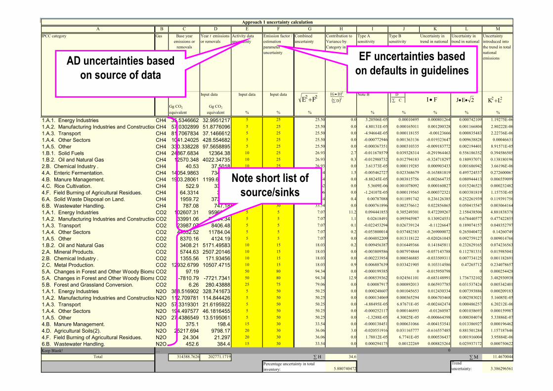
TABLE 3.2 APPROACH 1 UNCERTAINTY CALCULATION

A B C D E F G H I J K L M

IPCC category

Gas Base year emissions or removals

Year t emissions or removals

Activity data uncertainty

Emission factor / estimation parameter uncertainty

Combined uncertainty

Contribution to Variance by Category in Year t

Type A sensitivity

Type B sensitivity

Uncertainty in trend in national emissions introduced by emission factor / estimation parameter uncertainty

Uncertainty in trend in national emissions introduced by activity data uncertainty

Uncertainty introduced into the trend in total national emissions

Input data Input data Input data Note A

Input data Note A

22 FE

2

2

D

DG

Note B

CD

FI

Note C 2EJ

Note D

22 LK

Gg CO2 equivalent

Gg CO2 equivalent % % % % % % % %

E.g., 1.A.1. Energy Industries Fuel 1

CO2

E.g., 1.A.1. Energy Industries Fuel 2

CO2

Etc... …

Total C D H M

Percentage uncertainty in total inventory: H Trend uncertainty: M

Enter Emissions Data

Enter Uncertainties

Data Calculated using simple equations

Approach 1: Error Propagation

A B C D E F G H I J K L MIPCC category Gas Base year

emissions or removals

Year t emissions or removals

Activity data uncertainty

Emission factor / estimation parameter uncertainty

Combined uncertainty

Contribution to Variance by Category in Year t

Type A sensitivity

Type B sensitivity

Uncertainty in trend in national emissions introduced by emission factor / estimation parameter uncertainty

Uncertainty in trend in national emissions introduced by activity data uncertainty

Uncertainty introduced into the trend in total national emissions

Input data Input data Input data Input data Note B

Gg CO2

equivalentGg CO2

equivalent % % % % % % % %

1.A.1. Energy Industries CH4 35.5346662 32.9951217 5 25 25.50 0.0 3.20506E-05 0.00010495 0.000801264 0.000742109 1.19275E-06

1.A.2. Manufacturing Industries and ConstructionCH4 57.0302899 51.8776096 5 25 25.50 0.0 4.80131E-05 0.000165011 0.001200328 0.001166804 2.80222E-06

1.A.3. Transport CH4 81.7067834 37.1466612 5 25 25.50 0.0 -4.94664E-05 0.000118155 -0.00123666 0.000835483 2.22736E-06

1.A.4. Other Sectors CH4 1041.24025 428.554682 5 25 25.50 0.0 -0.000772946 0.001363136 -0.019323647 0.009638828 0.00046631

1.A.5. Other CH4 330.338228 97.5658895 5 25 25.50 0.0 -0.000367351 0.000310335 -0.009183772 0.002194401 8.91571E-05

1.B.1. Solid Fuels CH4 24867.6834 12364.38 10 25 26.93 2.7 -0.011678579 0.039328314 -0.291964463 0.556186352 0.394586505

1.B.2. Oil and Natural Gas CH4 12570.348 4022.34735 10 25 26.93 0.3 -0.012988732 0.012794183 -0.324718297 0.180937071 0.138180196

2.B. Chemical Industry . CH4 40.53 37.5018 10 25 26.93 0.0 3.61373E-05 0.000119285 0.000903433 0.001686942 3.66196E-06

4.A. Enteric Fermentation. CH4 14054.9863 7346.85 15 30 33.54 1.5 -0.005462727 0.023368679 -0.163881819 0.495724537 0.272600067

4.B. Manure Management. CH4 1903.28061 1199.63088 15 30 33.54 0.0 -8.88245E-05 0.003815756 -0.002664735 0.080944413 0.006559099

4.C. Rice Cultivation. CH4 522.9 338.94 10 30 31.62 0.0 5.3609E-06 0.001078092 0.000160827 0.015246523 0.000232482

4.F. Field Burning of Agricultural Residues. CH4 64.3314 37.59 20 30 36.06 0.0 -1.24107E-05 0.000119565 -0.000372321 0.003381819 1.15753E-05

6.A. Solid Waste Disposal on Land. CH4 1959.72 3738.63 15 30 33.54 0.4 0.00787088 0.011891742 0.236126385 0.252261939 0.119391756

6.B. Wastewater Handling. CH4 787.08 747.18 15 30 33.54 0.0 0.000761896 0.002376612 0.022856865 0.050415547 0.003064164

1.A.1. Energy Industries CO2 102607.31 95966.95 5 5 7.07 11.2 0.094441853 0.305249301 0.472209267 2.158438506 4.881838378

1.A.2. Manufacturing Industries and ConstructionCO2 33991.06 30164.34 5 5 7.07 1.1 0.02618491 0.095945987 0.130924551 0.678440577 0.477422855

1.A.3. Transport CO2 23987.07 8406.48 5 5 7.07 0.1 -0.022453294 0.026739124 -0.11226647 0.189074157 0.048352797

1.A.4. Other Sectors CO2 44532.52 11784.04 5 5 7.07 0.2 -0.053800014 0.037482383 -0.269000072 0.265040472 0.14260749

1.A.5. Other CO2 8370.16 4124.19 5 5 7.07 0.0 -0.004052209 0.013118122 -0.020261045 0.092759127 0.009014766

1.B.2. Oil and Natural Gas CO2 3408.21 5171.49583 10 15 18.03 0.2 0.009456387 0.016449366 0.141845811 0.232629165 0.074236563

2.A. Mineral Products. CO2 5744.63 2507.20146 10 15 18.03 0.0 -0.003809586 0.007974844 -0.057143788 0.112781331 0.015985041

2.B. Chemical Industry . CO2 1355.56 171.93456 10 15 18.03 0.0 -0.002233954 0.000546885 -0.033509311 0.007734125 0.001182691

2.C. Metal Production. CO2 12932.6799 10507.4715 10 15 18.03 0.9 0.006887639 0.033421905 0.103314586 0.47265712 0.234078657

5.A. Changes in Forest and Other Woody BiomaCO2 97.19 50 80 94.34 0.0 -0.000199385 0 -0.015950798 0 0.000254428

5.A. Changes in Forest and Other Woody BiomaCO2 -7810.79 -7721.7341 50 80 94.34 12.9 -0.008539362 0.024561101 -0.683148991 1.736732102 3.482930938

5.B. Forest and Grassland Conversion. CO2 6.26 280.43888 25 75 79.06 0.0 0.00087917 0.000892013 0.065937785 0.031537424 0.005342401

1.A.1. Energy Industries N2O 388.516902 328.741673 5 50 50.25 0.0 0.000248607 0.001045653 0.012430334 0.007393886 0.000209183

1.A.2. Manufacturing Industries and ConstructionN2O 112.709781 114.844426 5 50 50.25 0.0 0.000134069 0.000365294 0.006703468 0.002583021 5.16085E-05

1.A.3. Transport N2O 57.3319301 21.6195922 5 50 50.25 0.0 -4.88495E-05 6.87671E-05 -0.002442474 0.000486257 6.20212E-06

1.A.4. Other Sectors N2O 194.497577 46.1816455 5 50 50.25 0.0 -0.000252117 0.000146893 -0.01260587 0.001038693 0.000159987

1.A.5. Other N2O 27.4386549 13.5195061 5 50 50.25 0.0 -1.3288E-05 4.30025E-05 -0.000664398 0.000304074 5.33886E-07

4.B. Manure Management. N2O 375.1 198.4 15 30 33.54 0.0 -0.000138451 0.000631066 -0.004153541 0.013386927 0.000196462

4.D. Agricultural Soils(2). N2O 25217.694 9798.17 20 30 36.06 3.0 -0.020551916 0.031165777 -0.616557485 0.881501284 1.157187646

4.F. Field Burning of Agricultural Residues. N2O 24.304 21.297 20 30 36.06 0.0 1.78812E-05 6.7741E-05 0.000536437 0.001916004 3.95884E-06

6.B. Wastewater Handling. N2O 452.6 384.4 15 30 33.54 0.0 0.000294175 0.00122269 0.008825264 0.025937172 0.000750622

Keep Blank! … 0Total 314388.7626 202771.1719 34.6 11.4670044

5.880740472Trend uncertainty: 3.386296561

Percentage uncertainty in total inventory:

Approach 1 uncertainty calculation

22 FE 2

2

D

DG

CD

FI 2EJ 22 LK

H M

Note short list of source/sinks

EF uncertainties based on defaults in guidelines

AD uncertainties based on source of data

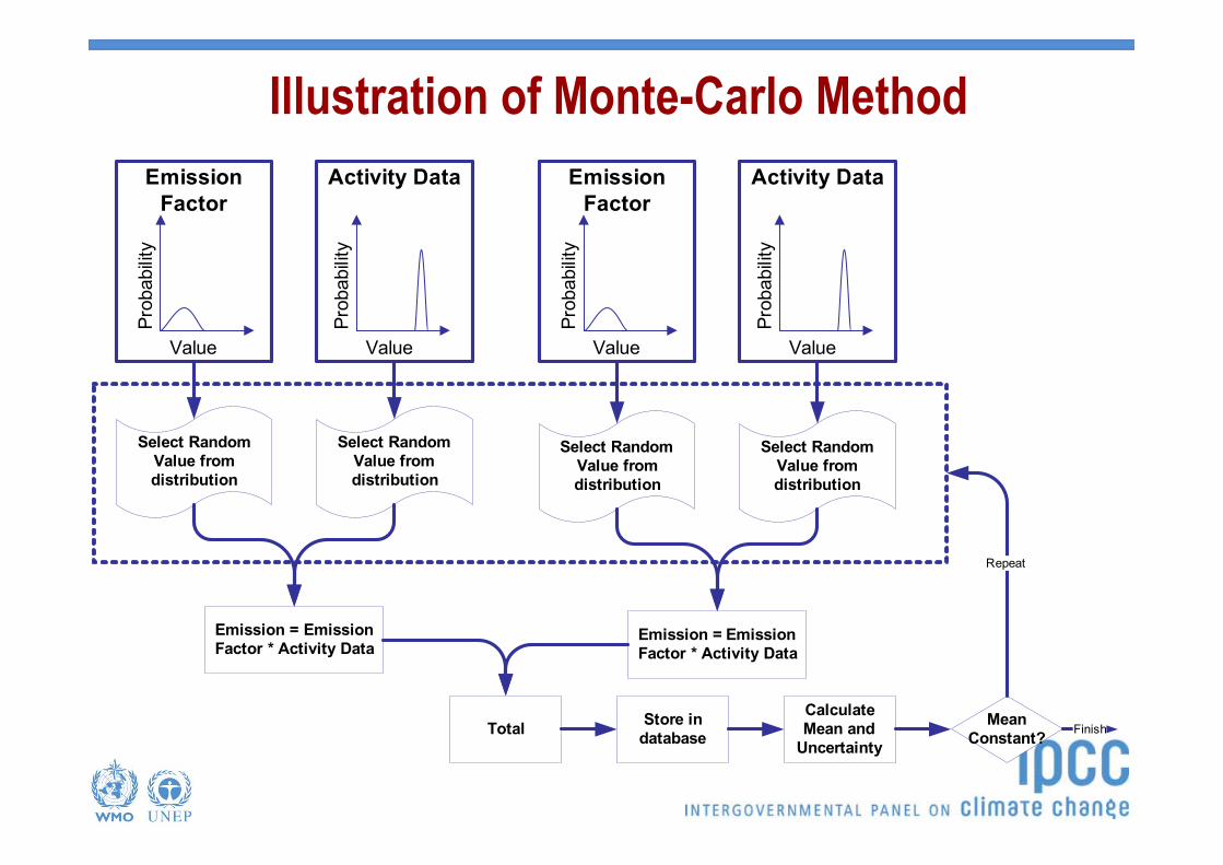
Approach 2: Monte Carlo Method• Key Requirements

– Not just uncertainties but also probability density function (pdf)• Mean• Width• Shape (e.g. Normal, Log-normal, Weibul, Gamma, Uniform,

Triangular, Fractile, …)• Principle

– Select random values of input parameters from their pdf and calculate the corresponding emission. Repeat many times and the distribution of the results is the pdf of the result, from which mean and uncertainty can be estimated

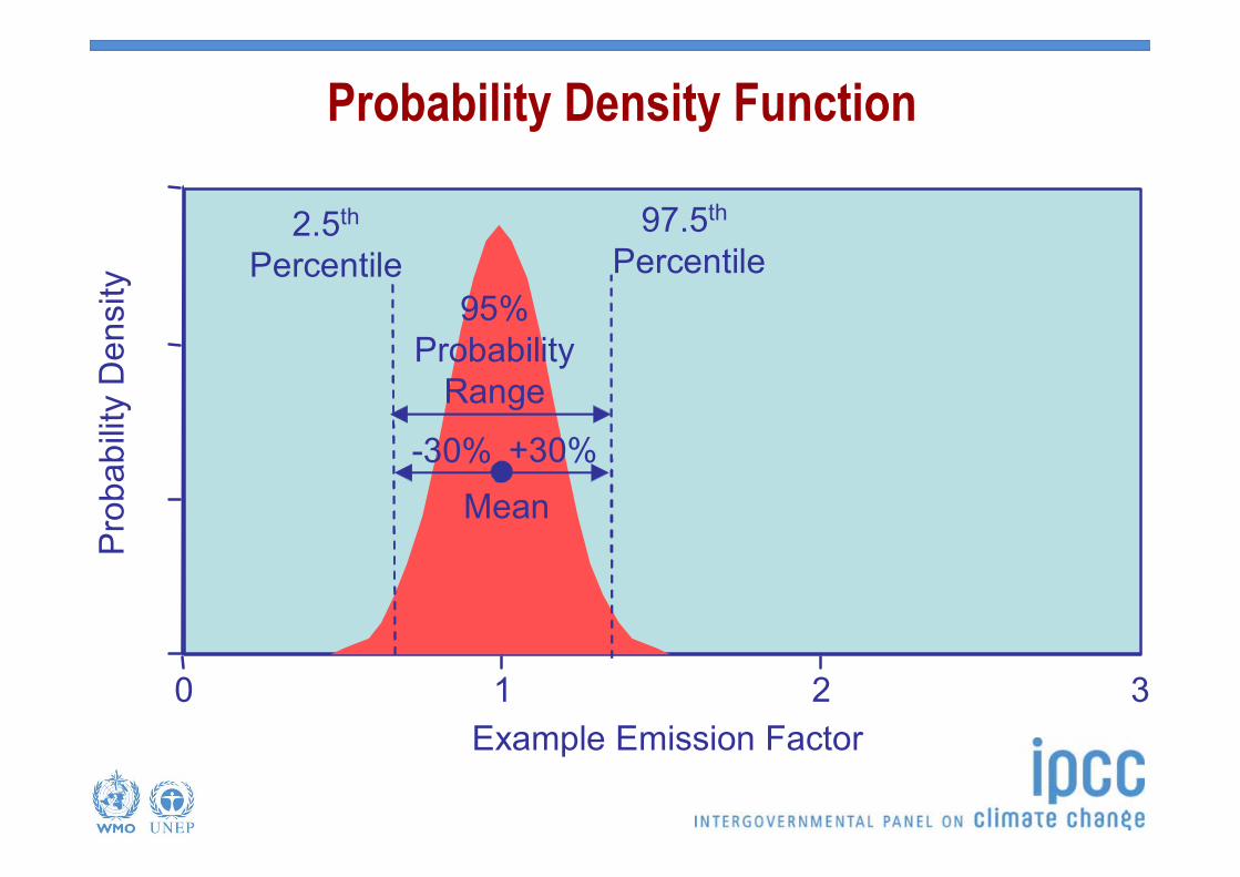
Probability Density Function

0 1 2 3Example Emission Factor

Pro

babi

lity

Den

sity

97.5th

Percentile2.5th

Percentile

Mean-30% +30%

95%Probability

Range

Probability Density Function

0 1 2 3Example Emission Factor

Pro

babi

lity

Den

sity 95% Probability Range

Mean-50% +100%

97.5th

Percentile2.5th

Percentile

Value

Prob

abilit

y

ValuePr

obab

ility

Emission Factor

Activity Data

Emission = Emission Factor * Activity Data

Select Random Value from distribution

Select Random Value from distribution

Value

Prob

abilit

y

Value

Prob

abilit

y

Emission Factor

Activity Data

Emission = Emission Factor * Activity Data

Select Random Value from distribution

Select Random Value from distribution

TotalCalculate Mean and

Uncertainty

Store in database

Mean Constant?

Repeat

Finish

Illustration of Monte-Carlo Method

Example of Monte Carlo Results

0

0.2

0.4

0.6

0.8

1

1.2

0.85 0.9 0.95 1 1.05Millions

Emission

Freq

uenc

y

1 Runs

0

0.5

1

1.5

2

2.5

3

3.5

4

4.5

0.85 0.9 0.95 1 1.05Millions

Emission

Freq

uenc

y

10 Runs

0

0.5

1

1.5

2

2.5

3

3.5

0.85 0.9 0.95 1 1.05Millions

Emission

Freq

uenc

y

20 Runs

0

1

2

3

4

5

6

7

8

0.85 0.9 0.95 1 1.05Millions

Emission

Freq

uenc

y

50 Runs

0

2

4

6

8

10

12

14

0.85 0.9 0.95 1 1.05Millions

Emission

Freq

uenc

y

100 Runs

0

10

20

30

40

50

60

0.85 0.9 0.95 1 1.05Millions

Emission

Freq

uenc

y

500 Runs

0

20

40

60

80

100

120

0.85 0.9 0.95 1 1.05Millions

Emission

Freq

uenc

y

1000 Runs

0

100

200

300

400

500

600

0.85 0.9 0.95 1 1.05Millions

Emission

Freq

uenc

y

5000 Runs

0

200

400

600

800

1000

1200

0.85 0.9 0.95 1 1.05Millions

Emission

Freq

uenc

y

10000 Runs

Summary Results

880000

900000

920000

940000

960000

980000

1000000

1020000

1 10 20 50 100 500 1000 5000 10000

Number of Runs

Em

issi

on

Mean2.5 percentile97.5 percentile

Click “Uncertainty Analysis”

Click to perform analysis

Uncertainty Analysis: IPCC Inventory Software

Click to enter AD and EF uncertainties

Uncertainty Analysis: IPCC Inventory Software (cont.)

Summary• Even simple uncertainty estimates give useful information - If they are

performed well• Assessment of uncertainty in the input parameters should be part of the data

collection – Careful consideration will improve estimates as well as providing input

data for uncertainty analysis• If resources limited: effort spent on uncertainty analysis should be small

compared with total effort

• At its simplest a well planned uncertainty assessment should only take a few extra hours!– Uncertainty in AD assessed as data collected– Uncertainty in EFs from guidelines now available– Aggregate categories/gases to independent groups of sources/sinks– Use Approach 1

Thank you

Diagrams © IPCC unless otherwise noted