Beyond Attributes -> Describing Images Tamara L. Berg UNC Chapel Hill.
Upload
rosamond-hortonCategory
view
216download
0
UNC Chapel Hill M. C. Lin
Introduction to Motion Planning
Applications Overview of the Problem Basics – Planning for Point Robot
– Visibility Graphs– Roadmap– Cell Decomposition– Potential Field

UNC Chapel Hill M. C. Lin
Goals
Compute motion strategies, e.g.,– Geometric paths – Time-parameterized trajectories– Sequence of sensor-based motion commands
Achieve high-level goals, e.g.,– Go to the door and do not collide with obstacles– Assemble/disassemble the engine– Build a map of the hallway– Find and track the target (an intruder, a missing
pet, etc.)

UNC Chapel Hill M. C. Lin
Fundamental Question
Are two given points connected by a path?

UNC Chapel Hill M. C. Lin
Basic Problem
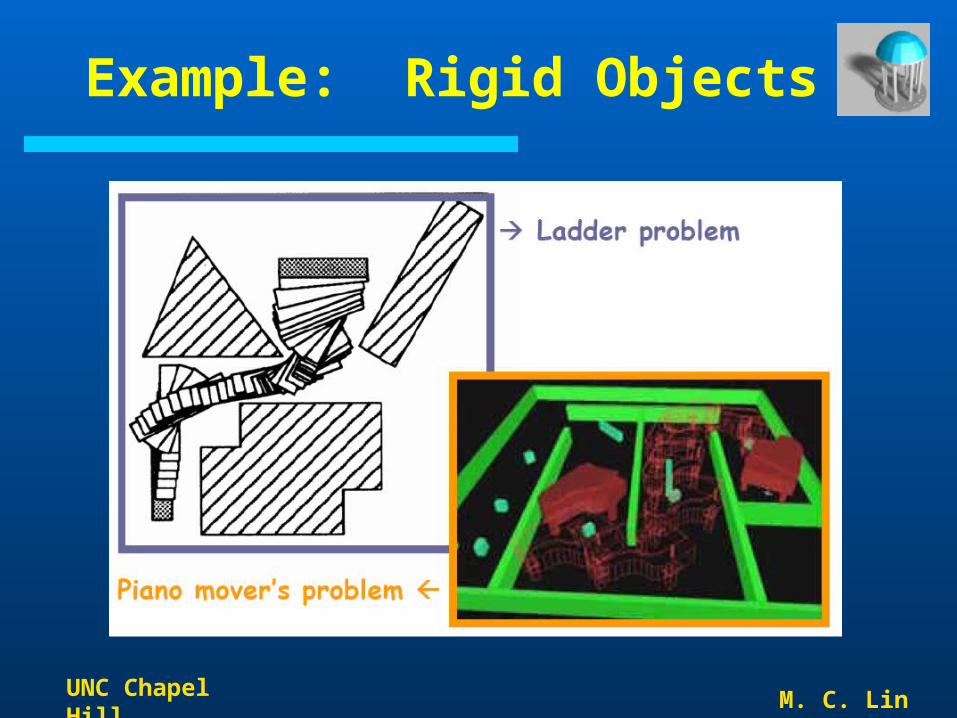
Problem statement: Compute a collision-free pathfor a rigid or articulated
moving object among static obstacles. Input
– Geometry of a moving object (a robot, a digital actor, or a molecule) and obstacles
– How does the robot move?– Kinematics of the robot (degrees of freedom)– Initial and goal robot configurations (positions & orientations)
Output Continuous sequence of collision-free robot
configurations connecting the initial and goal configurations
UNC Chapel Hill M. C. Lin
Example: Rigid Objects

UNC Chapel Hill M. C. Lin
Example: Articulated Robot

UNC Chapel Hill M. C. Lin
Is it easy?

UNC Chapel Hill M. C. Lin
Hardness Results
Several variants of the path planning problem have been proven to be PSPACE-hard.
A complete algorithm may take exponential time.– A complete algorithm finds a path if one exists and
reports no path exists otherwise.
Examples– Planar linkages [Hopcroftet al., 1984]– Multiple rectangles [Hopcroftet al., 1984]

UNC Chapel Hill M. C. Lin
Tool: Configuration Space
Difficulty– Number of degrees of freedom (dimension
of configuration space)– Geometric complexity
UNC Chapel Hill M. C. Lin
Extensions of the Basic Problem
More complex robots– Multiple robots– Movable objects– Nonholonomic& dynamic constraints– Physical models and deformable objects– Sensorlessmotions (exploiting task mechanics)– Uncertainty in control

UNC Chapel Hill M. C. Lin
Extensions of the Basic Problem
More complex environments– Moving obstacles– Uncertainty in sensing
More complex objectives– Optimal motion planning– Integration of planning and control– Assembly planning– Sensing the environment
• Model building• Target finding, tracking

UNC Chapel Hill M. C. Lin
Next Few Lectures
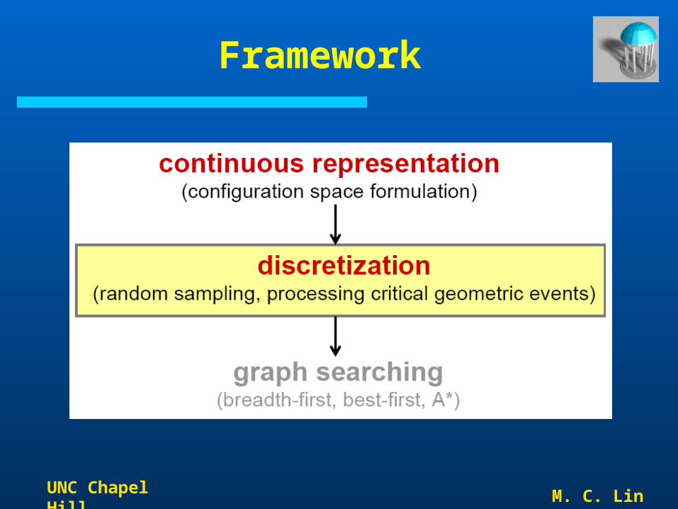
Present a coherent framework for motion planning problems:– Configuration space and related concepts– Algorithms based on random sampling and
algorithms based on processing critical geometric events
Emphasize “practical” algorithms with some guarantees of performance over “theoretical” or purely “heuristic” algorithms

UNC Chapel Hill M. C. Lin
Practical Algorithms
A complete motion planner always returns a solution when one exists and indicates that no such solution exists otherwise.
Most motion planning problems are hard, meaning that complete planners take exponential time in the number of degrees of freedom, moving objects, etc.
UNC Chapel Hill M. C. Lin
Practical Algorithms
Theoretical algorithms strive for completeness and low worst-case complexity– Difficult to implement– Not robust
Heuristic algorithms strive for efficiency in commonly encountered situations. – No performance guarantee
Practical algorithms with performance guarantees– Weaker forms of completeness– Simplifying assumptions on the space: “exponential
time” algorithms that work in practice

UNC Chapel Hill M. C. Lin
Problem Formulation for Point Robot
Input– Robot represented
as a point in the plane
– Obstacles represented as polygons
– Initial and goal positions
Output– A collision-free path
between the initial and goal positions
UNC Chapel Hill M. C. Lin
Framework

UNC Chapel Hill M. C. Lin
Visibility Graph Method
Observation: If there is a a collision-free path between two points, then there is a polygonal path that bends only at the obstacles vertices.
Why? – Any collision-free path
can be transformed into a polygonal path that bends only at the obstacle vertices.
A polygonal path is a piecewise linear curve.

UNC Chapel Hill M. C. Lin
Visibility Graph
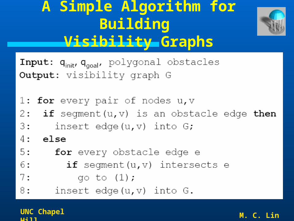
A visibility graphis a graph such that– Nodes: qinit, qgoal, or an obstacle vertex.– Edges: An edge exists between nodes u and v if the
line segment between u and v is an obstacle edge or it does not intersect the obstacles.
UNC Chapel Hill M. C. Lin
A Simple Algorithm for Building Visibility Graphs

UNC Chapel Hill M. C. Lin
Computational Efficiency
Simple algorithm O(n3) time More efficient algorithms
– Rotational sweep O(n2log n) time– Optimal algorithm O(n2) time– Output sensitive algorithms
O(n2) space

UNC Chapel Hill M. C. Lin
Framework
UNC Chapel Hill M. C. Lin
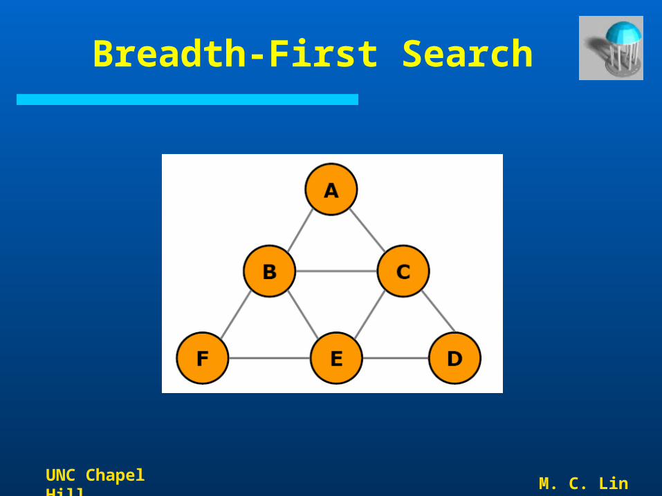
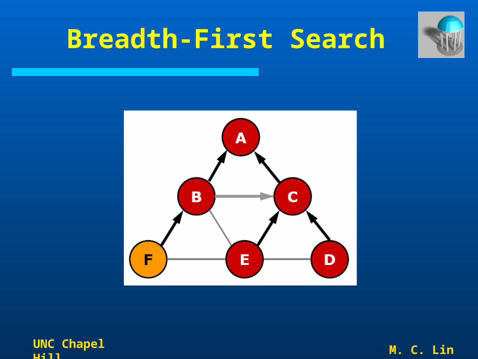
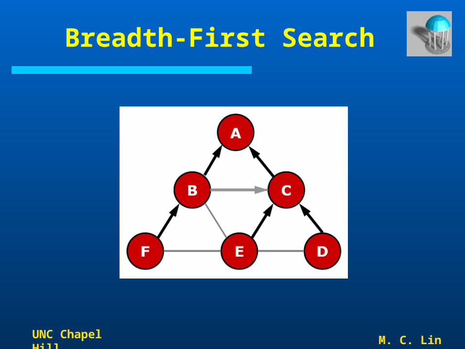
Breadth-First Search

UNC Chapel Hill M. C. Lin
Breadth-First Search

UNC Chapel Hill M. C. Lin
Breadth-First Search

UNC Chapel Hill M. C. Lin
Breadth-First Search

UNC Chapel Hill M. C. Lin
Breadth-First Search

UNC Chapel Hill M. C. Lin
Breadth-First Search
UNC Chapel Hill M. C. Lin
Breadth-First Search
UNC Chapel Hill M. C. Lin
Breadth-First Search

UNC Chapel Hill M. C. Lin
Breadth-First Search

UNC Chapel Hill M. C. Lin
Breadth-First Search

UNC Chapel Hill M. C. Lin
Other Search Algorithms
Depth-First SearchBest-First Search, A*

UNC Chapel Hill M. C. Lin
Framework

UNC Chapel Hill M. C. Lin
Summary
Discretize the space by constructing visibility graph
Search the visibility graph with breadth-first search
Q: How to perform the intersection test?

UNC Chapel Hill M. C. Lin
Summary
Represent the connectivity of the configuration space in the visibility graph
Running time O(n3)– Compute the visibility graph– Search the graph– An optimal O(n2) time algorithm exists.
Space O(n2)
Can we do better?

UNC Chapel Hill M. C. Lin
Classic Path Planning Approaches
Roadmap – Represent the connectivity of the free space by a network of 1-D curves
Cell decomposition – Decompose the free space into simple cells and represent the connectivity of the free space by the adjacency graph of these cells
Potential field – Define a potential function over the free space that has a global minimum at the goal and follow the steepest descent of the potential function
UNC Chapel Hill M. C. Lin
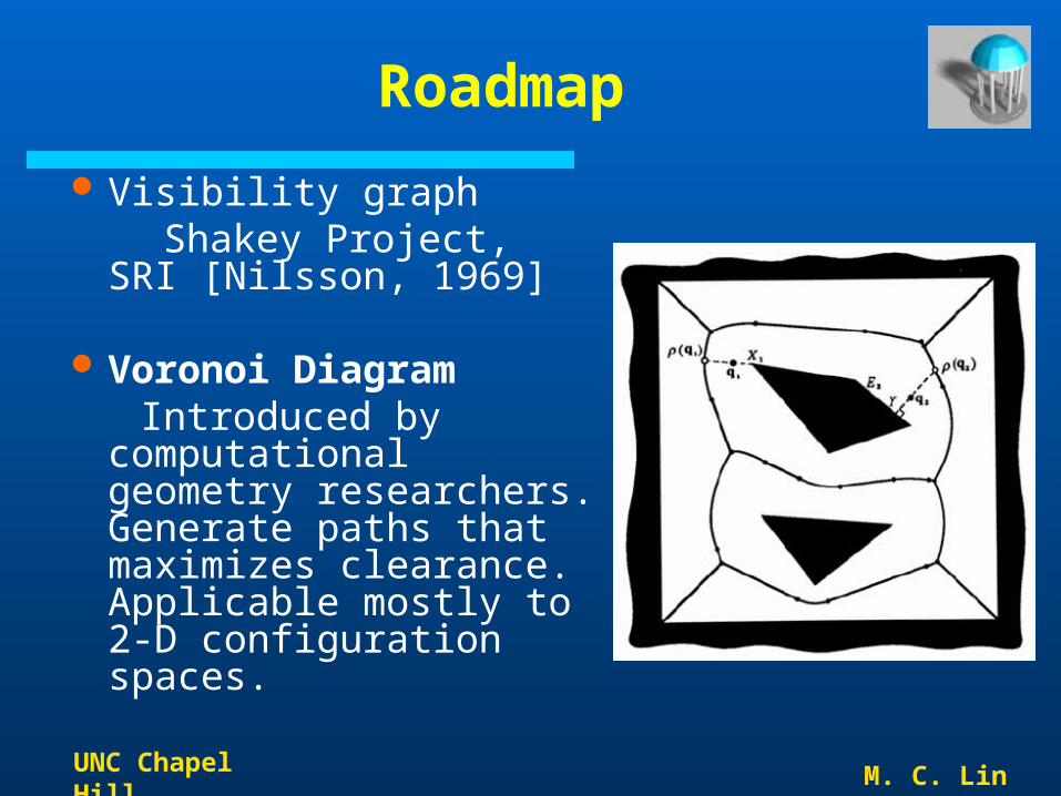
Roadmap
Visibility graph Shakey Project, SRI
[Nilsson, 1969]
Voronoi Diagram Introduced by
computational geometry researchers. Generate paths that maximizes clearance. Applicable mostly to 2-D configuration spaces.

UNC Chapel Hill M. C. Lin
Voronoi Diagram
Space O(n)Run time O(n log n)
UNC Chapel Hill M. C. Lin
Other Roadmap Methods
Silhouette
First complete general method that applies to spaces of any dimensions and is singly exponential in the number of dimensions [Canny 1987]
Probabilistic roadmaps

UNC Chapel Hill M. C. Lin
Classic Path Planning Approaches
Roadmap – Represent the connectivity of the free space by a network of 1-D curves
Cell decomposition – Decompose the free space into simple cells and represent the connectivity of the free space by the adjacency graph of these cells
Potential field – Define a potential function over the free space that has a global minimum at the goal and follow the steepest descent of the potential function

UNC Chapel Hill M. C. Lin
Cell-decomposition Methods
Exact cell decomposition
The free space F is represented by a collection of non-overlapping simple cells whose union is exactly F
Examples of cells: trapezoids, triangles

UNC Chapel Hill M. C. Lin
Trapezoidal Decomposition
UNC Chapel Hill M. C. Lin
Computational Efficiency
Running time O(n log n) by planar sweep
Space O(n)Mostly for 2-D configuration spaces

UNC Chapel Hill M. C. Lin
Adjacency Graph
Nodes: cells Edges: There is an edge between every pair of
nodes whose corresponding cells are adjacent.
UNC Chapel Hill M. C. Lin
Summary
Discretize the space by constructing an adjacency graph of the cells
Search the adjacency graph

UNC Chapel Hill M. C. Lin
Cell-decomposition Methods
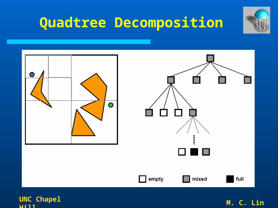
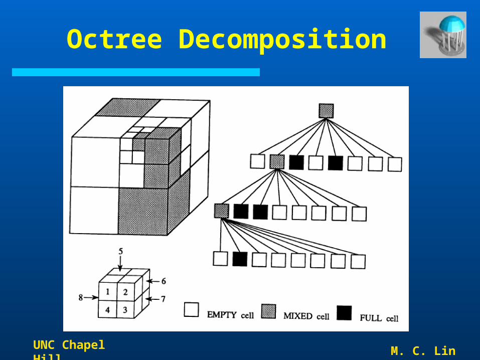
Exact cell decompositionApproximate cell decomposition
– F is represented by a collection of non-overlapping cells whose union is contained in F.
– Cells usually have simple, regular shapes, e.g., rectangles, squares.
– Facilitate hierarchical space decomposition
UNC Chapel Hill M. C. Lin
Quadtree Decomposition
UNC Chapel Hill M. C. Lin
Octree Decomposition

UNC Chapel Hill M. C. Lin
Algorithm Outline
UNC Chapel Hill M. C. Lin
Classic Path Planning Approaches
Roadmap – Represent the connectivity of the free space by a network of 1-D curves
Cell decomposition – Decompose the free space into simple cells and represent the connectivity of the free space by the adjacency graph of these cells
Potential field – Define a potential function over the free space that has a global minimum at the goal and follow the steepest descent of the potential function

UNC Chapel Hill M. C. Lin
Potential Fields
Initially proposed for real-time collision avoidance [Khatib 1986]. Hundreds of papers published.
A potential field is a scalar function over the free space.
To navigate, the robot applies a force proportional to the negated gradient of the potential field.
A navigation function is an ideal potential field that– has global minimum at the goal– has no local minima– grows to infinity near obstacles– is smooth

UNC Chapel Hill M. C. Lin
Attractive & Repulsive Fields

UNC Chapel Hill M. C. Lin
How Does It Work?
UNC Chapel Hill M. C. Lin
Algorithm Outline
Place a regular grid G over the configuration space
Compute the potential field over GSearch G using a best-first algorithm
with potential field as the heuristic function

UNC Chapel Hill M. C. Lin
Local Minima
What can we do?– Escape from local minima by taking
random walks– Build an ideal potential field – navigation
function – that does not have local minima

UNC Chapel Hill M. C. Lin
Question
Can such an ideal potential field be constructed efficiently in general?

UNC Chapel Hill M. C. Lin
Completeness
A complete motion planner always returns a solution when one exists and indicates that no such solution exists otherwise.– Is the visibility graph algorithm complete?
Yes.– How about the exact cell decomposition
algorithm and the potential field algorithm?