Unbiased LiDAR Data Measurement (Draft)

Ty Naus, Fugro Horizons, Inc.

Abstract When describing a LiDAR dataset, many aspects are unambiguous such as the area of coverage or the acquisition date. Additional characteristic values of accuracy and error typically accompany the data and well-defined guidelines exist for how these values should be derived and reported. Two supplementary characterizations are frequently used, namely Nominal Spacing and Density, for which there is no standardized method on how they should be derived and reported. A statistical bias is easily introduced when providing spacing and density quantification. A method of measurement is presented in which spacing and density statistics can be qualified and bias identified. The law of large numbers certainly applies to datasets with millions or billions of points and means that the variance can be reduced, but not the bias. While it may appear trivial, the principal contributors to LiDAR spacing and density bias are the absence of clear and concise definitions. Bias can not be entirely eliminated but should be reduced wherever possible. Introduction LiDAR point spacing and point density is often referred to in the literature and other publicly available sources as a means of quantifying and qualifying this type of data (FEMA, 2002, Gueudet, 2004, NOAA). Additional qualification results when the term “nominal” is applied to the spacing value, however by definition, nominal may have no real relation to the item being referred to (Wikipedia). Descriptive terms for LiDAR points and their spatial properties are also referred to as “postings” or “post-spacing” or “spot spacing”. Point Spacing is identified as being an important aspect in a national LiDAR survey (Stoker et al., 2007) and density is cited numerous times by different organizations in that report. According to the Encyclopedia Britannica, “One of the chief problems with statistics is the ability to make them say what one desires through the manipulation of numbers or graphics.” Any effort of the scale and magnitude like a national LiDAR survey will have to contend with the problem of statistical manipulation or bias that is either intentional or unintentional. Spatial data resolution is a concern when LiDAR data is processed to DEM’s for use in hydrologic modeling for floodplain delineation (Omer et al., 2003), water fluxes and balances (Bormann, 2006), or other geographic applications (Cowen et al., 2000). There are well-established specifications for determination of accuracy (FEMA, 2003, Flood, 2004) and other industry standard guidelines for Digital Elevation Data (Maune, 2001). To date, there is very little guidance as to how representative values of point spacing and density from LiDAR data should be determined and reported. It is difficult to characterize a LiDAR dataset because of the numerous variables such as localized terrain

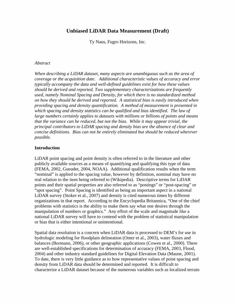
undulations (Kelley, 2006). LiDAR point density is not as intuitively understood as DEM or image resolution and most systems do not give a symmetrical point pattern (Rost, 2008). King County, Washington has elaborated on their method of point density determination, using a 100 square meter polygon and point counts of ground classified points within it. Kobler and Ogrinic (2007) provide several density values based on LiDAR pulse returns and combinations of returns. Publishing the actual density appears to be the exception and not the rule. Point Distribution Patterns There are numerous factors affecting the actual distribution of LiDAR pulse returns. These include instrument characteristics with associated parameters, terrain, and environmental conditions. Point spacing and density can be theoretically determined when only instrument and idealized platform characteristics are considered because the spacing is a function of the laser pulse frequency, the scan frequency and the flight height (Baltsavias, 1999). Differences in LiDAR system design result in different scan patterns including sinusoidal, zig-zag, parallel, and elliptical (Flood, 2001). Actual or real-world data points show variable spacing with values that are smaller or larger than a nominal spacing specified in a LiDAR project (Giglierano, 2007). Cumulative conditions result in deviation of point distribution over a surface and may approach uniform theoretical conditions for certain terrain types such as flat, open fields at or near nadir, whereas pattern irregularity from “grid-like” distribution is typically observed in areas of substantial terrain relief and dense vegetation. Pattern irregularity tends to increase with incident angle or scan angle toward the edge of the field of view and in the case of LiDAR systems that produce sinusoidal scan patters, is a function of mirror velocity. An unbiased measurement technique must be equally applicable to these conditions as it is to a theoretical condition. Hereafter, it will be useful to have a real world example and for this a small portion of the much larger Red River Basin Mapping Initiative (RRBMI) was chosen. This approximately 40,000 square mile project includes the entire US portion of the Red River Basin in North Dakota, Minnesota and South Dakota. The LiDAR data will ultimately be available to the public on the US Geological Survey’s website and consist of an estimated 56.2 billion points. Figure 1a shows the theoretical model of point distribution near nadir and Figure 1b shows the distribution at the edge of the swath where 10% side lap has been removed. The model and actual RRBMI data are oriented with a flight direction that is North – South. This model is based on simple harmonic motion and a single oscillating mirror LiDAR system and in accordance with the mission flight plan for the RRBMI, a 45-degree field of view, a flight height 8,000 feet above the mean terrain elevation, an airspeed of 165 knots, a pulse rate of 94,000 Hz and a mirror scan rate of 33.1 Hz.

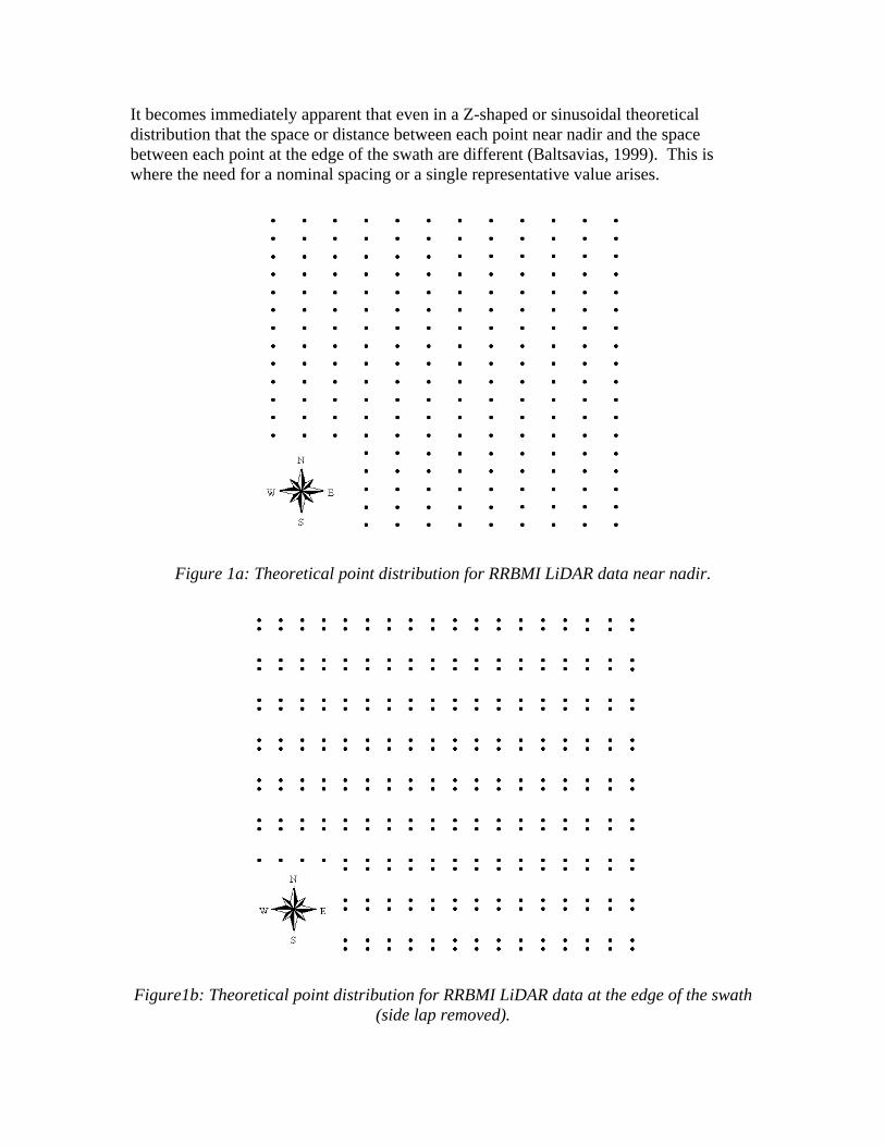
It becomes immediately apparent that even in a Z-shaped or sinusoidal theoretical distribution that the space or distance between each point near nadir and the space between each point at the edge of the swath are different (Baltsavias, 1999). This is where the need for a nominal spacing or a single representative value arises.

Figure 1a: Theoretical point distribution for RRBMI LiDAR data near nadir.

Figure1b: Theoretical point distribution for RRBMI LiDAR data at the edge of the swath

(side lap removed).

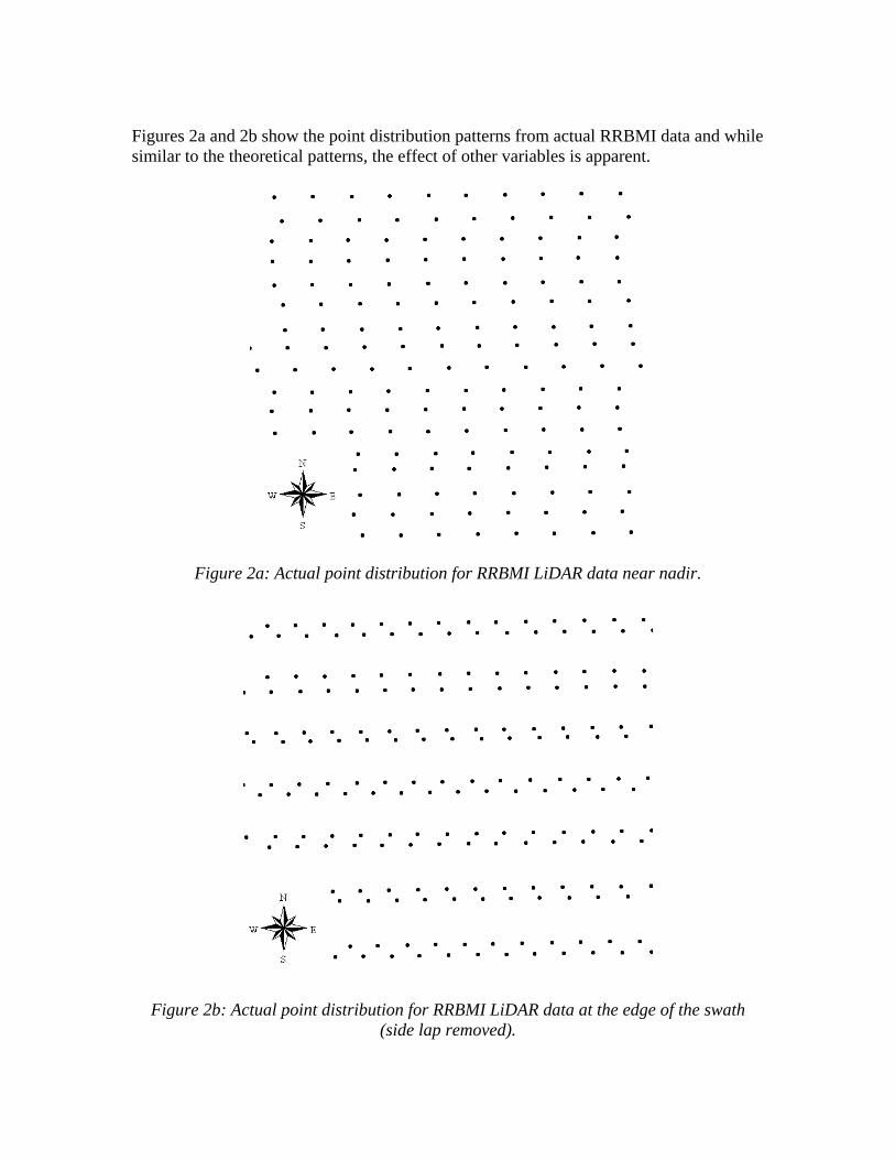
Figures 2a and 2b show the point distribution patterns from actual RRBMI data and while similar to the theoretical patterns, the effect of other variables is apparent.

Figure 2a: Actual point distribution for RRBMI LiDAR data near nadir.

Figure 2b: Actual point distribution for RRBMI LiDAR data at the edge of the swath (side lap removed).

Point Spacing Point spacing refers to 1-dimensional measurement or a point-to-point distance. Recognizing that point distributions are not regularly or evenly spaced it is quite uncommon to find a single point that has an equal distance to all of the points surrounding it so that a nominal spacing would be some generalized value that attempts to quantify this. The scan patterns of several different types of instruments result in directionally dependent spacing or two distinct orientations associated with flight orientation (Baltsavias, 1999). The numerous statistical methods available indicate that nominal point spacing can be derived from almost anything from an average to an approximate average (Raber, 2007) to potentially more elaborate equations with multiple parameters. Nominal measurement was first applied to statistics by Stanley Smith Stevens (1946) where it was suggested that nominal is a level in a classification scheme and is at the lowest level of mathematical structure. Stevens also suggested that nominal can define mode but within this type of measure median and mean do not exist. Statistical dispersion can be measured with Stevens’s definition, but no notion of standard deviation exists. This definition should not be applied to the distribution of LiDAR points on a surface since the most frequently encountered measurement (mode) is unlikely to have any meaning. The National Digital Elevation Program (NDEP) provides one definition of nominal post spacing as being “the smallest distance between two points that can be explicitly represented in a gridded elevation dataset” (NDEP, 2004). Even though the term is frequently encountered, most often, the method by which the stated nominal spacing value was or is derived is never indicated. Point Density Point density is related to point spacing and it is therefore logical that the closer a group of points are to one another, the higher the point density. Point density is often referred to in association with LiDAR data and not surprisingly, with few exceptions like King County, Washington (County, King 2003), the method and details by which the statistic was determined is absent. In most cases, it is difficult to determine if the reported density value is theoretically derived (Baltsavias, 1999) or calculated from actual data. If the King County method is representative of the method by which point density is determined, then it can be assumed that the value, unless additionally qualified, is derived from a “box counting” in which the area of a rectangle is associated with the total number of LiDAR points inside the rectangle. The problems related to this methodology are numerous but best illustrated by an “arbitrary box counting” example where the size or scale of the rectangle and its placement within a data set produce different density values. This phenomenon has been recognized previously (Levin, 1992, Raber, 2007) in other studies where varying scales

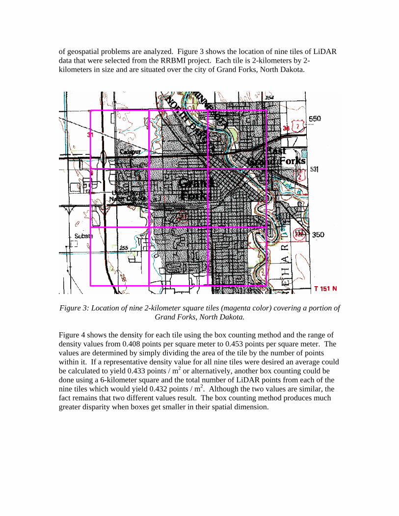
of geospatial problems are analyzed. Figure 3 shows the location of nine tiles of LiDAR data that were selected from the RRBMI project. Each tile is 2-kilometers by 2-kilometers in size and are situated over the city of Grand Forks, North Dakota.

Figure 3: Location of nine 2-kilometer square tiles (magenta color) covering a portion of

Grand Forks, North Dakota. Figure 4 shows the density for each tile using the box counting method and the range of density values from 0.408 points per square meter to 0.453 points per square meter. The values are determined by simply dividing the area of the tile by the number of points within it. If a representative density value for all nine tiles were desired an average could be calculated to yield 0.433 points / m2 or alternatively, another box counting could be done using a 6-kilometer square and the total number of LiDAR points from each of the nine tiles which would yield 0.432 points / m2. Although the two values are similar, the fact remains that two different values result. The box counting method produces much greater disparity when boxes get smaller in their spatial dimension.

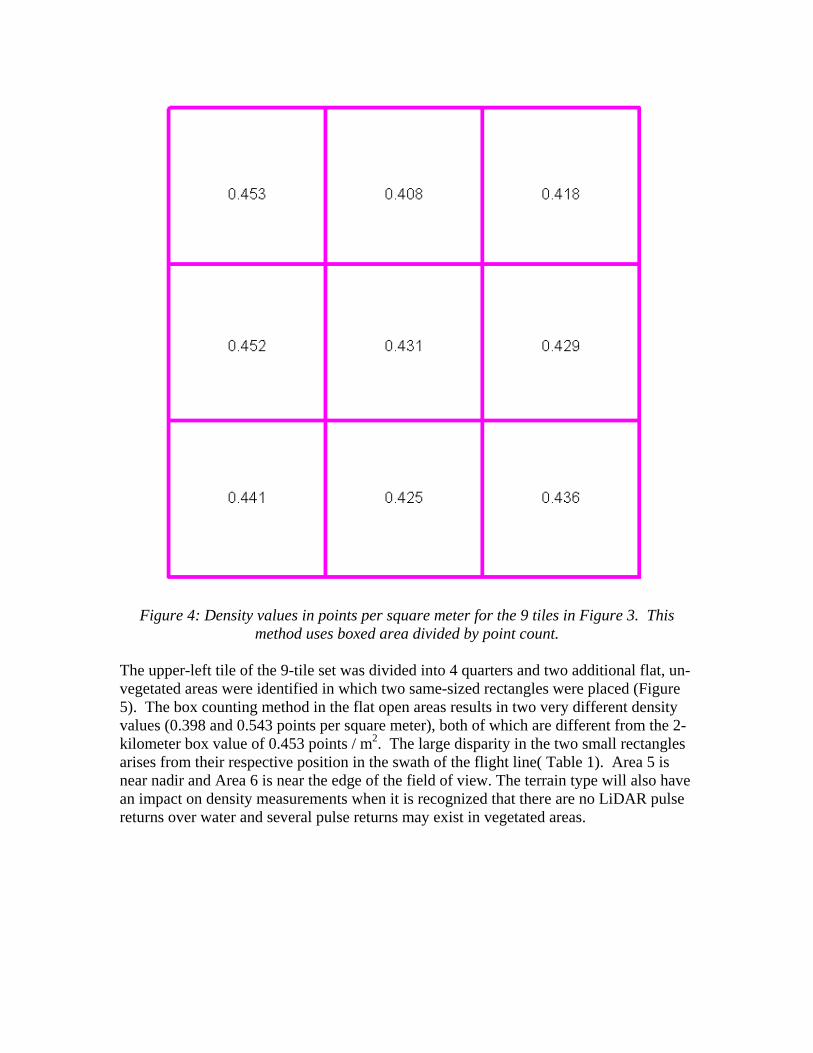
Figure 4: Density values in points per square meter for the 9 tiles in Figure 3. This method uses boxed area divided by point count.

The upper-left tile of the 9-tile set was divided into 4 quarters and two additional flat, un-vegetated areas were identified in which two same-sized rectangles were placed (Figure 5). The box counting method in the flat open areas results in two very different density values (0.398 and 0.543 points per square meter), both of which are different from the 2-kilometer box value of 0.453 points / m2. The large disparity in the two small rectangles arises from their respective position in the swath of the flight line( Table 1). Area 5 is near nadir and Area 6 is near the edge of the field of view. The terrain type will also have an impact on density measurements when it is recognized that there are no LiDAR pulse returns over water and several pulse returns may exist in vegetated areas.

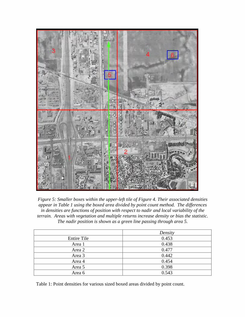
Figure 5: Smaller boxes within the upper-left tile of Figure 4. Their associated densities appear in Table 1 using the boxed area divided by point count method. The differences in densities are functions of position with respect to nadir and local variability of the

terrain. Areas with vegetation and multiple returns increase density or bias the statistic. The nadir position is shown as a green line passing through area 5.

Density

Entire Tile 0.453 Area 1 0.438 Area 2 0.477 Area 3 0.442 Area 4 0.454 Area 5 0.398 Area 6 0.543

Table 1: Point densities for various sized boxed areas divided by point count.

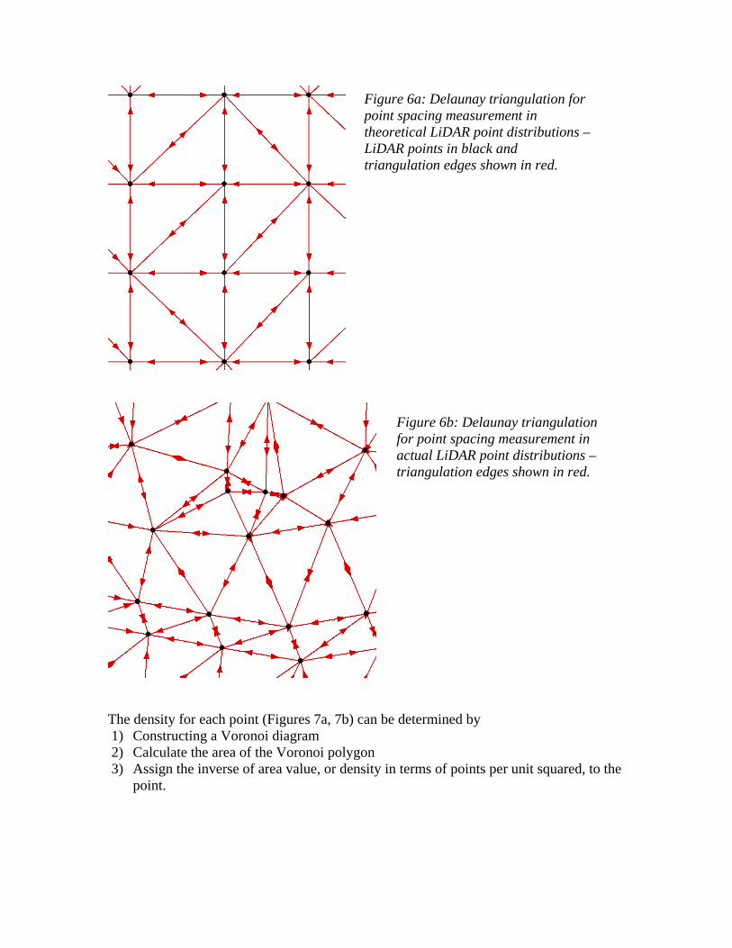
Unbiased Measurement There are numerous opportunities to introduce statistical bias into reported LiDAR point spacing and point density values. The bias does not necessarily have to be intentional and it is practically impossible to identify a perfectly random sample given the number of variables. Additionally, bias should not be associated with negative connotation. A reported point density for the entirety of a large LiDAR project is not representative of a subset of the data as illustrated by the box counting method at various scales. The LiDAR data would be underutilized if the area of interest was positioned accordingly with favorable terrain and ground cover conditions and the statistic for analysis was based on an entire project value that underestimated the density of the subset area. A well-defined measurement method is required so that terminology and quantification remains consistent within the industry and can be clearly communicated among data producers and end users. Shih and Huang (2006) recognized that there are different ways to present point density and proposed a TIN based solution. Building on this concept and utilizing Delaunay Triangulation and Voronoi Diagrams in the quantification process, several problematic issues related to spacing and density values can be addressed. This includes homogeneity between theoretical acquisition statistics and the actuality of point distributions as they are affected by environmental variables like terrain, ground cover and instrument characteristics. The duality between Delaunay Triangulation and the Voronoi Diagram has an additional benefit of providing a compatible inter-relationship between spacing and density and facilitates additional data analysis from LiDAR datasets based on repeatable statistics. Delaunay Triangulation provides a method by which each LiDAR point can have a unique spacing and density value. The arrangement of the points is inconsequential to the triangulation so that theoretical and actual data are measured in the same way. As it applies to LiDAR data, the notion of disparate distance from point to point with respect to along-track and across-track directions is eliminated. Recent advances in the computation of Delaunay Triangulations (Isenburg, 2006) facilitate triangulation of huge datasets and while it is not necessary to calculate the spacing and density at this scale, it could be used to provide a “pre-calculated” underlying geometry. Measurement of point spacing and point density can be accomplished in 3 steps for spacing and in 3 steps for density. The measurement method then becomes part of the definition of LiDAR point spacing and point density. For point spacing (Figures 6a, 6b)

1) Construct a Delaunay triangulation 2) Calculate the distance of every edge connecting one point to a neighbor point 3) Calculate the average of the edge lengths and assign it to that point

The density for each point (Figures 7a, 7b) can be determined by 1) Constructing a Voronoi diagram 2) Calculate the area of the Voronoi polygon 3) Assign the inverse of area value, or density in terms of points per unit squared, to the

point.

Figure 6a: Delaunay triangulation for point spacing measurement in theoretical LiDAR point distributions – LiDAR points in black and triangulation edges shown in red.

Figure 6b: Delaunay triangulation for point spacing measurement in actual LiDAR point distributions – triangulation edges shown in red.

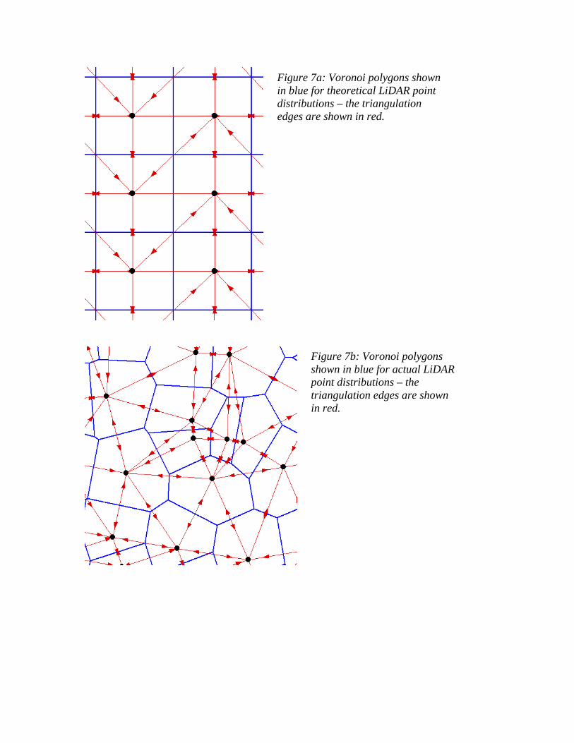
Figure 7a: Voronoi polygons shown in blue for theoretical LiDAR point distributions – the triangulation edges are shown in red.

Figure 7b: Voronoi polygons shown in blue for actual LiDAR point distributions – the triangulation edges are shown in red.

Defining Nominal Values Distribution statistics derived using the Delaunay / Voronoi measurement methods provide insight to the instrument and LiDAR acquisition project design. If it were possible to build a LiDAR instrument that could produce a perfectly symmetrical “grid” pattern at a 1-point per square meter density, the standard deviation, variance, skewness and kurtosis of that distribution would all be zero. In other words, every point in the population has the same value for spacing and for density. It could be accurately stated that the nominal value is the average value. In order to maintain consistency between theoretical and actual values and the way in which they are measured, a virtual model of the points can be constructed over an interval of time. The fundamental principals and equations for different system designs are detailed in Baltsavias (1999) and Wehr and Lohr (1999). The model should consist of an adequate number of points to support a triangulation from which internal points, or those points that are not members or “neighbors” of the set of convex hull points (Brown, 1979) are measured. These points are likely to skew the statistics and in practical application are typically within the region of flight line swath sidelap, or end lap. Absolute uniformity even theoretically is of course impossible, especially with respect to an instrument design where the resulting pattern is sinusoidal or zigzag. The instruments used for the RRBMI project produce sinusoidal point distributions and with the previously mentioned parameters show a non-normal distribution with significant positive skew for density and negative skew for spacing. Therefore providing an average value statistic for density and implying that it is representative is overestimating or biasing since the majority has lower density than the average. Considering that closer spacing is favorable over larger spacing, the negative skew for spacing says that an average spacing value is overestimating since more points are further from each other than the average value conveys. Once every point in the theoretical model has an associated, unique spacing and density value associated with it, the problem becomes one associated with scale, position and the number of points in a statistical quantification. Defining nominal values for a theoretical model could simply be a matter of extracting the points within the swath, accounting for side lap and using this point set for derived statistics. In this way the characteristics of the instrument and parameters of the project design dictate the nominal spacing and density. By sorting the lists of spacing and density values, useful values can be extracted from the model. Maximum values might be used as a threshold to identify voids in actual data in a quality control process or to perform an alternative check for normal distribution. Extracting the measured values from the sorted lists at 68%, 95% and 99.7% (empirical rule) and comparing them to the mean with the standard deviation can be another indication as to whether spacing and density are normally distributed.

The ASPRS recommends 95% percentile testing for vertical accuracy assessment (Flood, 2004). In keeping with the 95% confidence, as an example, a point set consisting of 10,000 points and sorted by spacing value from small to large, a nominal point spacing value can be qualified at 95% by extracting the value at the array index of 9,500. In the case of the RRBMI flight plan and resulting model, it can be stated that 95% of the points will have a spacing value of 2.091 meters or less or “the nominal spacing is 2.091 meters (95%)”. Nominal density can also be determined by this method resulting in 0.349 points per square meter (95%), or stated differently, 95% of the points are in areas where density is higher than 0.349 points /m2. Analyzing Actual Data Returning to the upper-left most tile of Figures 4 and 5, the measurement method was first applied to the entire tile and then to 4 separate quarters of the tile (Figure 8). The multiple return bias that was present in the initial arbitrary box counting method is eliminated by removing the first return of many and all intermediate returns. Only single returns and final returns are used. Each quarter can be generally characterized by terrain type where area 1 is mixed open area and light industrial, area 2 is moderately vegetated with data voids because of water, area 3 is similar to area 1 but with more open fields and area 4 is predominantly open fields. Areas 5 and 6 are characterized by flat, open terrain but are located at different positions with respect to nadir.

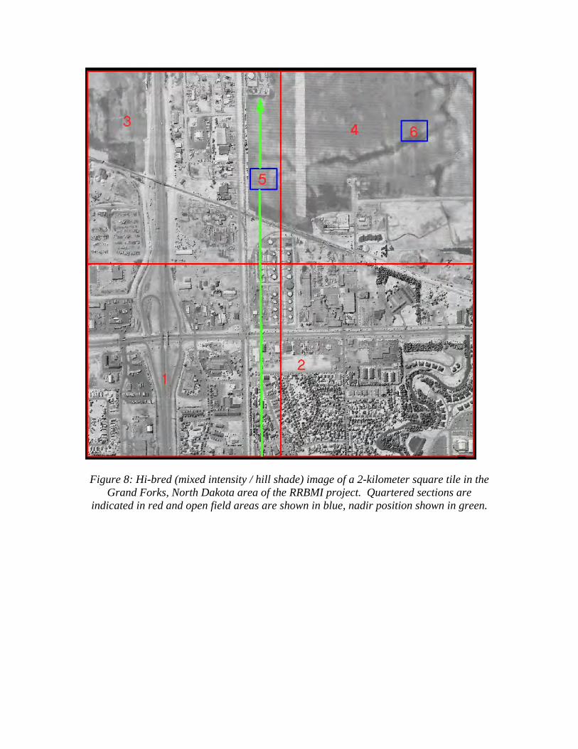
Figure 8: Hi-bred (mixed intensity / hill shade) image of a 2-kilometer square tile in the

Grand Forks, North Dakota area of the RRBMI project. Quartered sections are indicated in red and open field areas are shown in blue, nadir position shown in green.

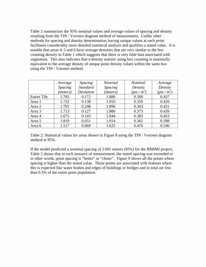
Table 2 summarizes the 95% nominal values and average values of spacing and density resulting from the TIN / Voronoi diagram method of measurement. Unlike other methods for spacing and density determination, having unique values at each point facilitates considerably more detailed statistical analysis and qualifies a stated value. It is notable that areas 4, 5 and 6 have average densities that are very similar to the box counting density in Table 1 which suggests that there is very little bias associated with vegetation. This also indicates that a density statistic using box counting is essentially equivalent to the average density of unique point density values within the same box using the TIN / Voronoi method. Average

Spacing (meters)

Spacing Standard Deviation

Nominal Spacing (meters)

Nominal Density

(pts / m2)

Average Density

(pts / m2) Entire Tile 1.705 0.172 1.886 0.368 0.437 Area 1 1.732 0.138 1.910 0.359 0.426 Area 2 1.701 0.248 1.896 0.363 0.431 Area 3 1.713 0.127 1.880 0.373 0.439 Area 4 1.675 0.143 1.844 0.383 0.453 Area 5 1.819 0.051 1.914 0.365 0.398 Area 6 1.517 0.069 1.625 0.476 0.546 Table 2: Statistical values for areas shown in Figure 8 using the TIN / Voronoi diagram method at 95%. If the model predicted a nominal spacing of 2.091 meters (95%) for the RRBMI project, Table 2 shows that in each instance of measurement, the stated spacing was exceeded or in other words, point spacing is “better” or “closer”. Figure 9 shows all the points where spacing is higher than the stated value. These points are associated with features where this is expected like water bodies and edges of buildings or bridges and in total are less than 0.5% of the entire point population.

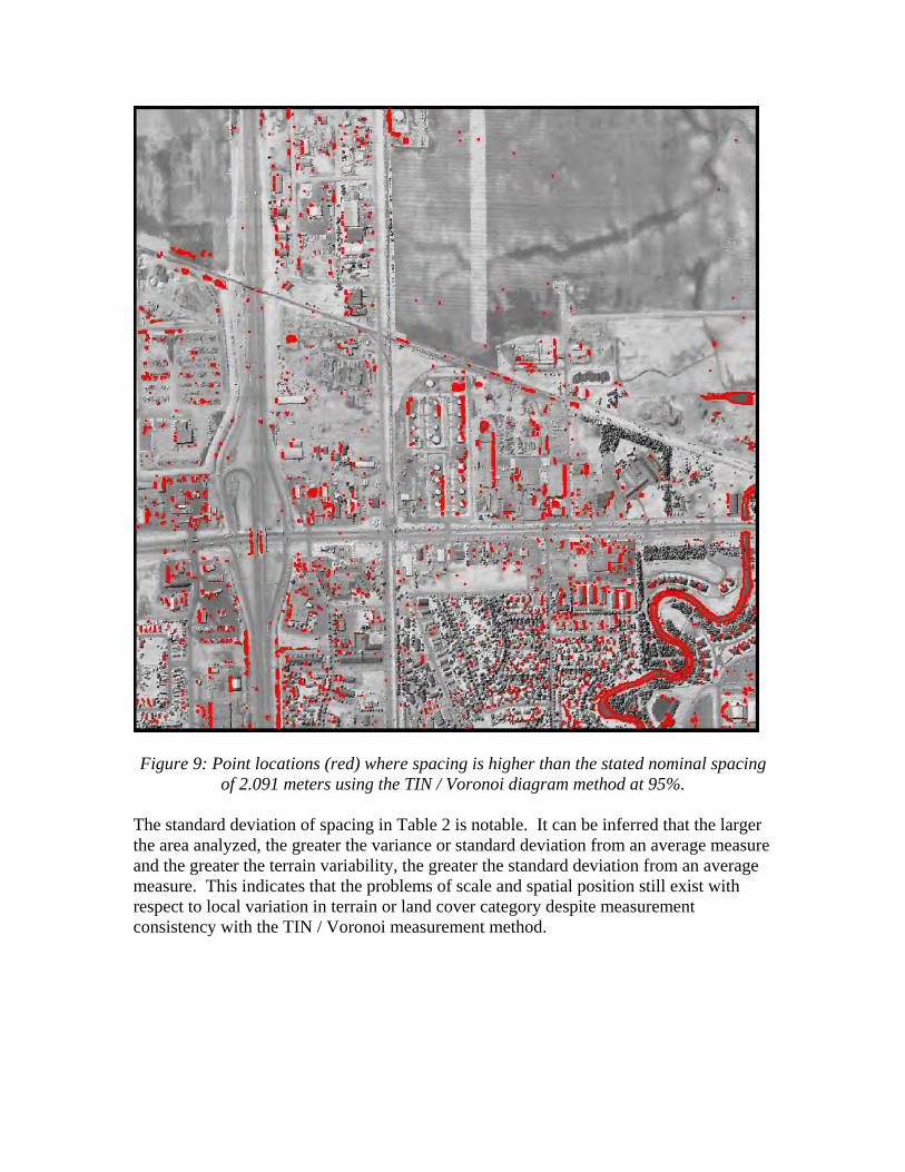
Figure 9: Point locations (red) where spacing is higher than the stated nominal spacing

of 2.091 meters using the TIN / Voronoi diagram method at 95%. The standard deviation of spacing in Table 2 is notable. It can be inferred that the larger the area analyzed, the greater the variance or standard deviation from an average measure and the greater the terrain variability, the greater the standard deviation from an average measure. This indicates that the problems of scale and spatial position still exist with respect to local variation in terrain or land cover category despite measurement consistency with the TIN / Voronoi measurement method.

Reporting Point Spacing and Density The guidelines for reporting accuracy (Flood, 2004, NDEP, 2004) are well established and provide a comprehensive method for making accuracy assessments. Topographic and ground cover variation are discussed as well as the selection and collection of checkpoints. It seems logical that a point spacing and density report could supplement an accuracy report. The TIN / Voronoi method of measurement provides unique values for each LiDAR point and is therefore scaled to the unique resolution of the data in the domain of each point. Characterizing datasets means that groups of points in larger areas must be used. Unbiased statistical quantification should minimize variability between samples and provide a simple and straightforward way to supply a characterization of the dataset regardless of its overall variability. It should also be applicable to the various scales and areas of interest that might be extracted from larger datasets. Multiple returns from a single pulse introduce bias into the statistics and cannot be anticipated in theoretical models and should not be used. Exceptions would apply to unique applications associated with vegetation such as those discussed in Renslow (2000) or Kobler (2007). For multiple returns, either the first or the last return should be used where the last return is preferred since it is more likely to be at the ground surface. Statistical measurement should not use only “Bare Earth” or ground classified points. This also introduces bias in the form of void areas associated with vegetation and buildings. Additional bias comes from varying perception and interpretation of ground points by automated classification algorithms and human editing (County, King, 2003). The ASPRS Vertical Accuracy guidelines for selection and placement of checkpoints could be followed for spacing and density characterization. Acknowledging that stated values from theoretical model distributions are measured on a flat plane and do not account for terrain or vegetation, a number of supplemental checkpoints can be collected throughout the dataset in flat, open areas. For the Grand Forks area, this was done within the nine tiles and is shown in Figure 10. Recognizing that smaller areas show less variance or standard deviation given consistency in the terrain condition (Table 2), the dimension of the area surrounding the checkpoint should be communicated in the metadata and the area should be rectangular in order to maintain consistency with presumed existing quantification methods like box counting for density.

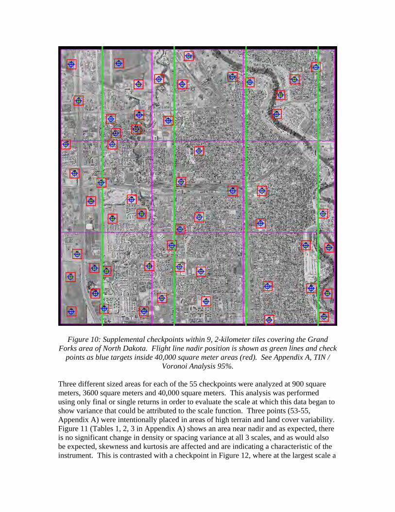
Figure 10: Supplemental checkpoints within 9, 2-kilometer tiles covering the Grand Forks area of North Dakota. Flight line nadir position is shown as green lines and check

points as blue targets inside 40,000 square meter areas (red). See Appendix A, TIN / Voronoi Analysis 95%.

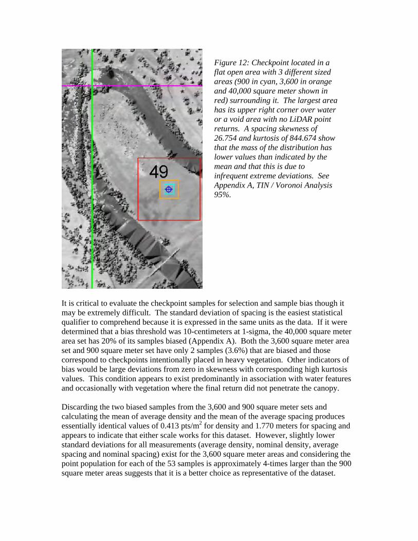
Three different sized areas for each of the 55 checkpoints were analyzed at 900 square meters, 3600 square meters and 40,000 square meters. This analysis was performed using only final or single returns in order to evaluate the scale at which this data began to show variance that could be attributed to the scale function. Three points (53-55, Appendix A) were intentionally placed in areas of high terrain and land cover variability. Figure 11 (Tables 1, 2, 3 in Appendix A) shows an area near nadir and as expected, there is no significant change in density or spacing variance at all 3 scales, and as would also be expected, skewness and kurtosis are affected and are indicating a characteristic of the instrument. This is contrasted with a checkpoint in Figure 12, where at the largest scale a

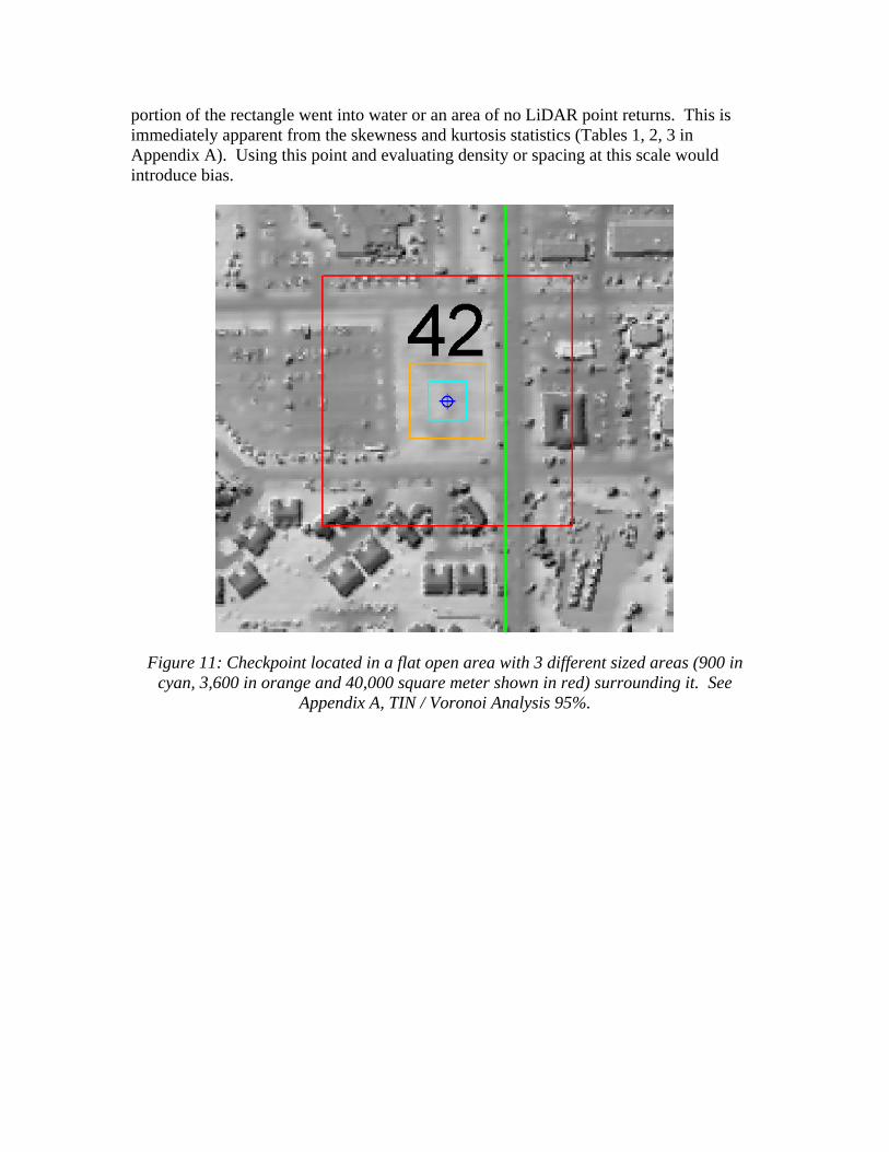
portion of the rectangle went into water or an area of no LiDAR point returns. This is immediately apparent from the skewness and kurtosis statistics (Tables 1, 2, 3 in Appendix A). Using this point and evaluating density or spacing at this scale would introduce bias.

Figure 11: Checkpoint located in a flat open area with 3 different sized areas (900 in cyan, 3,600 in orange and 40,000 square meter shown in red) surrounding it. See

Appendix A, TIN / Voronoi Analysis 95%.

It is critical to evaluate the checkpoint samples for selection and sample bias though it may be extremely difficult. The standard deviation of spacing is the easiest statistical qualifier to comprehend because it is expressed in the same units as the data. If it were determined that a bias threshold was 10-centimeters at 1-sigma, the 40,000 square meter area set has 20% of its samples biased (Appendix A). Both the 3,600 square meter area set and 900 square meter set have only 2 samples (3.6%) that are biased and those correspond to checkpoints intentionally placed in heavy vegetation. Other indicators of bias would be large deviations from zero in skewness with corresponding high kurtosis values. This condition appears to exist predominantly in association with water features and occasionally with vegetation where the final return did not penetrate the canopy. Discarding the two biased samples from the 3,600 and 900 square meter sets and calculating the mean of average density and the mean of the average spacing produces essentially identical values of 0.413 pts/m2 for density and 1.770 meters for spacing and appears to indicate that either scale works for this dataset. However, slightly lower standard deviations for all measurements (average density, nominal density, average spacing and nominal spacing) exist for the 3,600 square meter areas and considering the point population for each of the 53 samples is approximately 4-times larger than the 900 square meter areas suggests that it is a better choice as representative of the dataset.

Figure 12: Checkpoint located in a flat open area with 3 different sized areas (900 in cyan, 3,600 in orange and 40,000 square meter shown in red) surrounding it. The largest area has its upper right corner over water or a void area with no LiDAR point returns. A spacing skewness of 26.754 and kurtosis of 844.674 show that the mass of the distribution has lower values than indicated by the mean and that this is due to infrequent extreme deviations. See Appendix A, TIN / Voronoi Analysis 95%.

Summary and Conclusion Point density and nominal spacing are common descriptors of LiDAR data and are used with such frequency that their definitions and respective values are assumed to be common knowledge and are thus rarely, if ever qualified. Stated representative values without qualification invite questions of bias that are either intentional or unintentional. As far as can be determined, there is no standardized way to request LiDAR data at a given nominal spacing and density and then verify whether the actual data meets those specifications. First and foremost, there is no established definition of nominal as it applies to LiDAR point distributions. As point density increases so does the significance of the problem (20 centimeter variance at a 3-meter spacing is less significant than 20 centimeter variance at 1-meter spacing). It can be demonstrated that wide ranges of values can be produced when there is an underlying bias or combination of biases. These include but are not limited to:

• Area of coverage and size of the sample population • Instrument characteristics and associated point distribution patterns • Position of the sample with respect to airborne instrument position (e.g. nadir and

edge of swath) • Terrain variation (primarily percentage of area covered by water) • Ground cover variation and multiple pulse returns • Theoretically derived values or calculated using an undocumented method

A TIN / Voronoi Diagram based method provides a way in which theoretical and actual measurements can be similarly determined with an additional benefit of qualifying statistics that are standard techniques in the analysis of distributions. This method can also be used to define “nominal” with a consistent meaning regardless of theoretical condition or actual condition and is equally applicable to a normal (Gaussian) distribution as it is to a non-normal distribution. In an effort to standardize these parameters in the mapping community, the following terms have been suggested to identify 95% nominal values of spacing and density resulting from the TIN / Voronoi diagram method:

TIN / Voronoi - Average Spacing TIN / Voronoi - Spacing Standard Deviation TIN / Voronoi - Nominal Spacing (95%) TIN / Voronoi - Average Density TIN / Voronoi - Nominal Density (95%)

In the same mode as guidelines for the reporting of accuracy in LiDAR data, the method was applied to a subset of the Red River Basin Mapping Initiative LiDAR data and analyzed for its practical application with an emphasis on how a verification and reporting process could be established. If the LiDAR profession were to adopt this method of testing datasets, it would ensure that end customers get the product they are asking for and the data providers have an unbiased way of evaluating the data.

References Baltsavias, E.P., 1999, Airborne laser scanning: basic relations and formulas, ISPRS Journal of Photogrammetry and Remote Sensing, 54, 199-214 Bormann, H., 2006, Impact of spatial data resolution on simulated catchment water balances and model performance of the multi-scale TOPLATS model, Hydrology and Earth System Sciences, 10, 165–179 Brown, K. Q., 1979, Voronoi diagrams from convex hulls, Information Processing Letters 9(5), 223–228 County, King, 2003, LiDAR Digital Ground Model Point Density: King County, King County, WA. Cowen, D.J., Jensen, J.R., Hendrix, C., Hodgson, M.E. and Schill, S.R., 2000, A GIS-assisted Rail Construction Econometric Model that Incorporates LIDAR data, Photogrammetric Engineering & Remote Sensing, 66(11), 1323–1326 FEMA, 2002, LIDAR Specifications for Flood Hazard Mapping, Appendix 4B: Airborne Light Detection and Ranging Systems FEMA, 2003, Guidelines and Specifications for Flood Hazard Mapping Partners, Appendix A Flood, M., 2001, Laser Altimetry: From Science to Commercial Lidar Mapping, Photogrammetric Engineering & Remote Sensing, 67(11), 1209-1217 Flood, M. (Editor), 2004, ASPRS Guidelines Vertical Accuracy Reporting for Lidar Data V1.0, http://www.asprs.org/society/committees/lidar/Downloads/Vertical_Accuracy_Reporting_for_Lidar_Data.pdf Giglierano, J.D., 2007, Lidar Basics for Mapping Applications, US Geological Survey Open-File Report 2007-1285 Gueudet, Wells, Maidment, and Neuenschwander, 2004, Influence of the Post-Spacing Density of the LIDAR-Derived DEM on Flood Modeling, Proceedings of the 2004 American Water Resources Association Spring Conference Isenburg, M., Liu, Y., Shewchuk, J., and Snoeyink, J., 2006, Streaming Computation of Delaunay Triangulations, Proceedings of SIGGRAPH’06, 1049 – 1056

Kelley, D., and Loecherback, T., 2006, Challenges and Successes in Photogrammetric Approaches to LIDAR-Derived Products, MAPPS/ASPRS 2006 Fall Conference, November 6-10, 2006 San Antonio, Texas Kobler, A., and Ogrinc, P., 2007, REIN Algorithm and the Influence of Point Cloud Density on NDSM and DEM Precision in a Submediterranean Forest, ISPRS Workshop on Laser Scanning 2007 and SilviLaser 2007, Espoo, September 12-14, 2007, Finland Levin, S.A., 1992. The problem of pattern and scale in ecology, Ecology, 73(6), 1943–1967 Maune, D. (Editor), 2001, Digital Elevation Model Technologies and Application: The DEM Users Manual, ASPRS 2001, 540 pp. NDEP, 2004, Guidelines for Digital Elevation Data, Version 1.0, National Digital Elevation Program (NDEP), 93 pp. NOAA, Remote Sensing for Coastal Management, LIDAR, National Oceanic and Atmospheric Administration, Coastal Services Center, http://www.csc.noaa.gov/crs/rs_apps/sensors/lidar.htm Omer, C.R., Nelson, E.J., and Zundel, A.K., 2003. Impact of varied data resolution on hydraulic modeling and floodplain delineation, Journal of the American Water Resources Association, 39(2), 467–475

Raber, G. T., Jensen, J. R., Hodgson, M. E., Tullis, J. A., Davis, B. A., and Berglund, J., Impact of Lidar Nominal Post-spacing on DEM Accuracy and Flood Zone Delineation, Photogrammetric Engineering & Remote Sensing, 73(7), 793–804 Renslow, M., Greenfield, P. and Guay, T., 2000, Evaluation of Multi-retrun LIDAR for Forestry Applications, Project Report, US Department of Agriculture Forest Service – Engineering, Remote Sensing Applications Center, November 2000 Rost, H., and Grierson, H., 2008, High Precision Projects using LiDAR and Digitial Imagery, TS1I – Imaging and Data Applications, Integrating Generations, FIG Working Week 2008, Stockholm, Sweden 14-19 June 2008 Shih, P.T, and Huang, C.M., 2006, Abstract, Airborne Lidar Point Cloud Density Indices, American Geophysical Union, Fall Meeting 2006, abstract # G53C-0919 Stevens, S., 1946, On the theory of scales of measurement, Science, 103, 677-680 Stoker, J., Parrish, J., Gisclair, D., Harding, D., Haugerud, R., Flood, M., Andersen, H.E., Schuckman, K., Maune, D., Rooney, P., Waters, K., Habib, A., Wiggins, E., Ellingson, B., Jones, B., Nechero, S., Nayegandhi, A., Saultz, T., and Lee, G., Report of

the First National Lidar Initiative Meeting, February 14-16, 2007, Reston, Va., Report Series OF 2007-1189, U.S. Geological Survey Wehr, A., and Lohr, U., 1999, Airborne laser scanning—an introduction and overview, ISPRS Journal of Photogrammetry and Remote Sensing, 54, 68–82

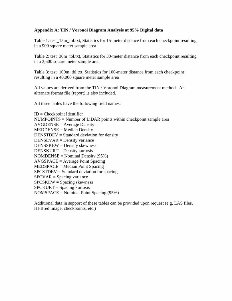
Appendix A: TIN / Voronoi Diagram Analysis at 95% Digital data Table 1: test_15m_tbl.txt, Statistics for 15-meter distance from each checkpoint resulting in a 900 square meter sample area Table 2: test_30m_tbl.txt, Statistics for 30-meter distance from each checkpoint resulting in a 3,600 square meter sample area Table 3: test_100m_tbl.txt, Statistics for 100-meter distance from each checkpoint resulting in a 40,000 square meter sample area All values are derived from the TIN / Voronoi Diagram measurement method. An alternate format file (report) is also included. All three tables have the following field names: ID = Checkpoint Identifier NUMPOINTS = Number of LiDAR points within checkpoint sample area AVGDENSE = Average Density MEDDENSE = Median Density DENSTDEV = Standard deviation for density DENSEVAR = Density variance DENSSKEW = Density skewness DENSKURT = Density kurtosis NOMDENSE = Nominal Density (95%) AVGSPACE = Average Point Spacing MEDSPACE = Median Point Spacing SPCSTDEV = Standard deviation for spacing SPCVAR = Spacing variance SPCSKEW = Spacing skewness SPCKURT = Spacing kurtosis NOMSPACE = Nominal Point Spacing (95%) Additional data in support of these tables can be provided upon request (e.g. LAS files, HI-Bred image, checkpoints, etc.)