Un it-1 E lasto-dy n am ics Uni t-1 · PDF fileUnit-1 Elasto-dynamics Page 4 Graphical...
38
Unit-1 Elasto-dynamics Page 1 Unit-1 Elasto-dynamics Syllabus: Simple Harmonic Motion, Electric Flux, displacement vector, Columb law, Gradient, Divergence, Curl, Gauss Theorem, Stokes theorem, Gauss law in dielectrics, Maxwell’s equation: Integral & Differential form in free space, isotropic dielectric medium. http://www.rgpvonline.com http://www.a2zsubjects.com
Transcript of Un it-1 E lasto-dy n am ics Uni t-1 · PDF fileUnit-1 Elasto-dynamics Page 4 Graphical...

Unit-1 Elasto-dynamics
Page 1
Unit-1
Elasto-dynamics
Syllabus:
Simple Harmonic Motion, Electric Flux, displacement vector, Columb law,
Gradient, Divergence, Curl, Gauss Theorem, Stokes theorem, Gauss law in
dielectrics, Maxwell’s equation: Integral & Differential form in free space,
isotropic dielectric medium.
http://www.rgpvonline.com http://www.a2zsubjects.com

Unit-1 Elasto-dynamics
Page 2
Periodic motion: If an object repeats its motion on a definite path after a regular time interval then such type of motion is
called periodic motion.
1) Vibratory motion or oscillatory motion
2) Uniform circular motion
3) Simple harmonic motion
Vibratory motion:
If a body in periodic motion moves to and fro about a definite point on a single path, the motion of the body
is said to be vibratory or oscillatory motion.
Mean or equilibrium position:
The point on either side of which the body vibrates is called the mean position or equilibrium position of the
motion.
Time period:
The definite time after which the object repeats its motion, is called time period and it is denoted by .
Frequency:
The number of complete oscillation in one second is called the frequency of that body, it is represented by
the letter or or � its unit is .
Uniform circular motion:
Figure(1): Uniform circular motion
Let an object is moving on a circular path of radius with uniform angular velocity � = .
http://www.rgpvonline.com http://www.a2zsubjects.com

Unit-1 Elasto-dynamics
Page 3
In right angle triangle Δ
∠ = � +� �
= cos � +� �
= cos � +� �
= .� cos � +� �
But � =
so = .� cos� � +� �
Similarly
= sin � +� �
= sin � +� �
= .� sin � +� �
= r.� sin� � +� �
Both equation (1) and (2) represents the uniform circular motion. Simple (armonic Motion S(M :
When a body moves periodically on a straight line on either side of a point, the motion is called the simple
harmonic motion.
http://www.rgpvonline.com http://www.a2zsubjects.com

Unit-1 Elasto-dynamics
Page 4
Graphical representation of SHM
Figure(2): Graphical representation of SHM
Displacement in SHM:
Let a particle is moving on a circular path with uniform angular velocity " " and the radius of the circular
path is " "; then movement of the point on their axis i.e. and is the SHM about the mean position
Figure(3): SHM
Let at time � =� the particle is on point and after time the position of the particle is then
In Δ
= sin
http://www.rgpvonline.com http://www.a2zsubjects.com

Unit-1 Elasto-dynamics
Page 5
= .� sin …………………………………………… (1)
= .� sin�
This equation represents the displacement of foot dropped from the position of particle on � −� .
Velocity in SHM:
Differentiating equation (1) with respect to we get-
= .� sin�
= rω cos� …………….
= √ � −� sin
= √ −� sin
= √ −� Using (1)
(i) In equilibrium condition � =� So
= √ −�
=
(ii) In the position of maximum displacement i.e. � =� So
= √ −�
=
Acceleration:
Again differentiating equation (2) we get-
=
�
= rω cos�
= −rω sin�
http://www.rgpvonline.com http://www.a2zsubjects.com

Unit-1 Elasto-dynamics
Page 6
= − ………………………………………………………… (3)
+� =
This is a second order differential equation which denotes the equation of SHM in the differential form
Again by equation (3)
= −
Multiplying by i.e. the mass of the particle executing SHM then
= −
= −
Here negative sing shows that the direction of displacement and acceleration are opposite to one another
So ∝ − � =�
Time period and frequency:
= ⇒ = √�
= √�
= √�
= √�
And = √�
Question: A uniform circular motion is given by the equation � =� � sin � +� ., find
1) Amplitude
2) Angular frequency
3) Time period
4) Phase
Sol: Given: � =� � sin� +� . Comparing the given equation with the standard equation of uniform circular motion i.e. � =� sin � +� �
http://www.rgpvonline.com http://www.a2zsubjects.com

Unit-1 Elasto-dynamics
Page 7
We get � =� � =� � � = = =� . � = = =� .
Question: A particle is moving with SHM in a straight line. When the displacement of the particle from
equilibrium position has values and , the corresponding position has valocities and
show that the time period of oscillation is given by
� =� √ −�−�
Sol: In the SHM the velocity is given by-
= √ −� …………………………………… (1)
At velocity is
So = √ −�
Squaring both sides
= −� …………………………. (2)
Again at the velocity is
So
= −� …………………………. (3)
By equation (2) and (3)
−� = −� � −� −�
−� = −�
−�−� =
http://www.rgpvonline.com http://www.a2zsubjects.com

Unit-1 Elasto-dynamics
Page 8
= −�−�
= √ −� −� …………………………. (4)
Now � =
So
= √ −�−�
Question: If the earth were a homogeneous sphere and a straight hole was bored in it through
the centre, then a body dropped in the hole, execute SHM. Calculate the time period
of its vibration. Radius of the earth is . � ×� 6 and � =� . −
Solution: The time period of oscillation executed by the body dropped in the hole along the
diameter of earth
� =� √=� √ . � ×� 6. =� .
Energy of a particle executing SHM:
A particle executing SHM possess potential energy on the account of its position and kinetic energy
on account of motion.
Potential energy:
We know that the acceleration in a simple harmonic motion is directly proportional to the displacement
and its direction is towards the mean position
= −
Let is the mass of particle executing SHM then the force acting on the particle will be-
= .�
= −
If the particle undergoes an infinitesimal displacement against the restoring force, then the small amount of
work done against the restoring force is given by
= − .�
Here negative sign shows that the restoring force is acting the displacement than
http://www.rgpvonline.com http://www.a2zsubjects.com
Unit-1 Elasto-dynamics
Page 9
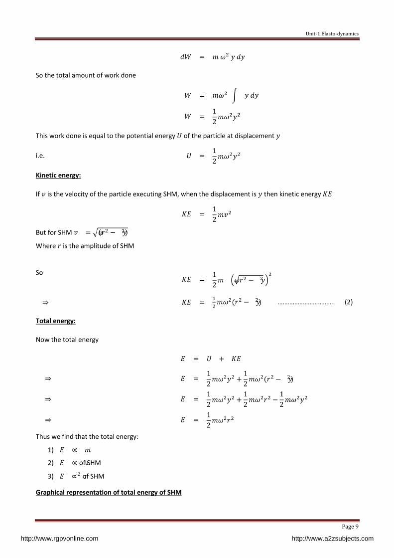
=
So the total amount of work done
= ∫�
=
This work done is equal to the potential energy of the particle at displacement
i.e. =
Kinetic energy:
If is the velocity of the particle executing SHM, when the displacement is then kinetic energy
=
But for SHM � =� √ −� Where is the amplitude of SHM
So
= � √ −�
⇒ = −� ……………………………. (2)
Total energy:
Now the total energy
= � +� ⇒ = + −�
⇒ = + −
⇒ =
Thus we find that the total energy:
1) � ∝�
2) � ∝� of SHM
3) � ∝� of SHM
Graphical representation of total energy of SHM
http://www.rgpvonline.com http://www.a2zsubjects.com

Unit-1 Elasto-dynamics
Page 10
Figure(4): Total energy of SHM
Position vector: A position vector expresses the position of a point P in space in terms of a displacement from an arbitrary
reference point O (typically the origin of a coordinate system). Namely, it indicates both the distance and
direction of an imaginary motion along a straight line from the reference position to the actual position of
the point. Displacement Vector: A displacement is the shortest distance from the
initial to the final position of a point P. Thus, it is
the length of an imaginary straight path, typically
distinct from the path actually travelled by
particle or object. A displacement vector
represents the length and direction of this
imaginary straight path.
Figure(5): Displacement vector Area Vector:
http://www.rgpvonline.com http://www.a2zsubjects.com

Unit-1 Elasto-dynamics
Page 11
In many problems the area is treated as a vector,
an area element is represented by , such
that the area representing the area vector is
perpendicular to the area element. The length of
the vector represents the magnitude of the
area element
Figure(6): Area vector
Coulomb’s Law: According to it the force of attraction or repulsion
between the two point charges is directly
proportional to the product of the magnitude of the
charges and inversely proportional to the square of
the distance between them.
If two charges and are separated at a distance
form one another then the force between these
charges will be-
Figure(7): Two electric charges separated a distance r
i) Force is proportional to the product of the magnitude of the charges i.e. � ∝� .�
ii) The force is inversely proportional to the distance between the charges i.e. � ∝
So � ∝ .� � =� .�
Where is a proportionality called electrostatic force constant, its value depends on the nature of the
medium in which the two charges are located and also the system of units adopted to measure ,� and .
So � =� ..�
http://www.rgpvonline.com http://www.a2zsubjects.com

Unit-1 Elasto-dynamics
Page 12
Case 1:(when the medium between the charges is air or vacuum )
As we know that the force between the charges is given as- � =� ..�
If we put =� =� and � =� then � =� So is the force feels by two charges of placed apart from one another in vacuum or free space.
Its value is � =� � �9 � � �
Case 2:(When the medium between the charges is other than the vacuum)
If the changes are located in any other medium then � = . =� � �9 .
Where is the dielectric constant of relative permittivity.
Putting this value in equation (1) we get
′ = . .�
Where ′ is the force in the medium
′ = . .�
Where � =� is called the relative permittivity of the medium.
Vector form of the Coulomb’s Law
Consider two like charges and present at and in vacuum at a distance apart. The two charges
will exert equal repulsive force on each other,
Let be the force on charge due to the charge and be the force on charge due to charge .
According to the Coulo s’ la , the ag itude of fo e o ha ge and is given by
| |. | | = .
………………………… (1)
Let and are the unit vectors in the direction from to and vice versa.
So the force is along the direction of unit vector , we have = . .�
http://www.rgpvonline.com http://www.a2zsubjects.com

Unit-1 Elasto-dynamics
Page 13
And = . .�
These two equations show the Coulo s’ la i e to fo .
Electric flux: Number of electric lines of forces passing normally through the surface, when held in the electric field. It is
denoted by � . There are two types of electric flux-
1. Positive electric flux: When electric lines of forces leave any body through its surface it is considered
as positive electric flux.
2. Negative electric flux: When lines of forces enter through any surface, it is considered as the
negative electric flux.
Measurement: Let us consider a small area of a
closed surface . The electric field produced
due to the charge will be radially outwards
which will be along . Now the normal to the
surface area is as shown in the figure,
hence the angle between and is �
So the electric lines of forces from the surface
area will be given as- � = .� � = � cos� �………….
Figure(8): Electric flux
Where � cos� � is the component of electric field along .
Hence the electric flux through a small elementary surface area is equal to the product of the small area and
normal component of along the direction of the elementary area . Over the hole surface, � = ∮ � cos� � � = ∮ .� ………………………… (2)
http://www.rgpvonline.com http://www.a2zsubjects.com

Unit-1 Elasto-dynamics
Page 14
Gradient of a scalar field: The gradient of a scalar function � is a vector whose magnitude
is equal to maximum rate of chcnge of scalar function � with
respect to the space variable ∇ and has direction along that
change. �� =�
In the scalar field let there be two level surfaces and close
together characterised by the scalar function � and �� +� �
respectively. Consider point and on the level surfaces and
respectively. Let and � +� be the position vector of and
. Then = =� � +� � +�
Now as � is a function of ,� ,� i.e.
�� =� � ,� ,�
Then the total differentiation of this function can be given as
Figure(9): Gradient of a scalar field
� = � � +� � +�
� = ( � +� � +� �)� .� ( � +� � +� )
� = ∇ � …………………………………………………… (1)
Agian if represents the distance along the normal from point to the surface to point , then
=
In the ∆
= cos� �
= cos� �
Now if we consider a unit vector along as
then
= .� …………………………………………………… (2)
If we proceed form to then value of scalar function � increases by an amount �
� = �
� = �� .� [Usi g ……………………………. (3)
http://www.rgpvonline.com http://www.a2zsubjects.com

Unit-1 Elasto-dynamics
Page 15
By equation (1) and (2)
(∇ .� �).� = �� .�
(∇ .� �) = ��
� = ��
Note:
∇ =� +� +� is called del or Nabla operator.
Note: � = ∇ .� � � = ( +� +� )� .� �
� = ( � +� � +� �)
Note: The gradient of a scalar field has great significant in physics. The negative gradient of
electric potential of electric field at a point represents the electric field at that point. i.e. =� − Note: The gradient of a scalar field is a vector quantity.
http://www.rgpvonline.com http://www.a2zsubjects.com

Unit-1 Elasto-dynamics
Page 16
Divergence of a vector field: The divergence of a vector field at a
certain point ,� ,� is defined as the
outward flux of the vector field per unit
volume enclosed through an infinitesimal
closed surface surrounding the point " ".
=� lim �→ .� �
=� lim �→ ��
Consider a infinitesimal rectangular box with
sides Δ ,� Δ ,� Δ and one corner at the point ,� ,� in the region of any vector
function with rectangular faces
perpendicular to co-ordinates axis.
Figure(10): divergence of a vector field
The flux emerging outwards from
surface i.� e.� surface , � = ∬ .�
� = ∬ ( +� +� ).� Δ ,� Δ
Where is the average of the vector function over the surface i.e. surface � = ∬ .� Δ .� Δ …………………………………………. (1)
Similarly
The flux emerging out from the
surface i.e. surface ,� � = ∬ .�
� = ∬ ( +� +� ).� − Δ ,� Δ
� = ∬ − .� Δ .� Δ ………………………………………. (2)
Thus net outwards flux of vector through the two faces perpendicular to � −axis,
http://www.rgpvonline.com http://www.a2zsubjects.com

Unit-1 Elasto-dynamics
Page 17
� = � +� � � = ∬ −� Δ .� Δ ……………….. (3)
But −� = � +� Δ ,� ,�−� ,� ,�
−� = Δ …………………………………………………… (4)
Where �� is the variation of with distance along � −axis by equation (2) and (3)
Thus net outward flux of vector function through the two faces perpendicular to � −axis
� = �� Δ Δ ,� Δ [ Using equation (3)
Similarly perpendicular to � −axis
� = Δ Δ Δ
Similarly perpendicular to � −axis
� = Δ Δ Δ
Therefore whole outward flux through infinitesimal box
� = � +� �+� �
� = + + Δ Δ Δ
Now at any point, which is the flux enclosed per unit infinitesimal volume surrounding that point is
given by-
= lim Δ Δ Δ → �Δ Δ Δ
= lim Δ Δ Δ → ( + + )� Δ Δ ΔΔ Δ Δ
= + +
= ( +� +� ) ( +� +� )
= ∇ .�
Note: Divergence of a vector field is a scalar quantity.
Note: If =� +
http://www.rgpvonline.com http://www.a2zsubjects.com

Unit-1 Elasto-dynamics
Page 18
it indicates the existence of the source of fluid at that point.
Note: If =� −
It means fluid is flowing towards the point and thus there exist a sink for the fluid.
Note: If =�
It means the fluid is flowing continuously from that point. In other words this means that the flux of
the vector function entering and leaving this region is equal. This condition is called solenoidal
vector.
http://www.rgpvonline.com http://www.a2zsubjects.com

Unit-1 Elasto-dynamics
Page 19
Curl of a vector field: If is any vector field at any point and an
infinitesimal test area at point then =� lim→ ∮ .�
Let us consider an infinitesimal rectangular area
with sides Δ and Δ parallel to � −� plane in the region of vector function . Let the coordinate of be ,� ,� . If ,� ,� are the Cartesian components of
at then =� +� +�
Figure(11): Curl of a vector field
Now the line integral of vector field
along the path = ∫� .�
= ( +� +� ).� Δ
= Δ
Where is the average value of � −component of the vector function over the path
Similarly for the Path
= ∫� .�
= ( +� +� ).� − Δ
= − Δ
Where is the average value of � −component of vector function over the path .
Hence the contribution to line integral ∮ . form two path and parallel to � −axis is
= −
= − − Δ
As the rectangle is infinitesimal the difference between the average of .� . − along these two
paths may be approximated to the difference between the values of at and
Thus-
− = −�
− = ,� � +� Δ ,�−� ,� ,�
http://www.rgpvonline.com http://www.a2zsubjects.com

Unit-1 Elasto-dynamics
Page 20
− = Δ
Hence the contribution to the line integral ∮ .� from the path and
= Δ Δ …………………………………………… (2)
Similarly by the path and
= Δ Δ …………………………………………… (3)
Therefore the line integral along the whole rectangular form (2) and (3) is given by-
= ∮� +� .�
= ∮� .�
= − Δ Δ ……………………………… (4)
Now = limΔ Δ →
= limΔ Δ → ( − )� Δ ΔΔ Δ
= − ……………………………………. (5)
Similarly
= ( − ) ……………………………………. (6)
and = − ……………………………………. (7)
Summing up the results given in (5), (6) and (7) we get
= +� +�
= � ( − )� +� � (− )� +� ( − )
= [
]
= ∇ ×�
Note: The curl of a vector field is sometime called circulation or rotation or simply .
http://www.rgpvonline.com http://www.a2zsubjects.com

Unit-1 Elasto-dynamics
Page 21
Note: If =� then vector field is called Lamellar field.
http://www.rgpvonline.com http://www.a2zsubjects.com

Unit-1 Elasto-dynamics
Page 22
Gauss’ Divergence Theorem: According to this theorem the volume integral of
divergence of a vector field over a volume is
equal to the surface integral of that vector field taken over the surface which enclosed that
volume . i.e. ∭( ) � =� ∬� .� �
Consider a volume enclosed by a surface this
volume can be divided into small elements of
volumes ,� …� …�� which are enclosed by the
elementary surface ,� …� …� …� …��
respectively. By definition the flux of a vector
field diverging out of the ℎ element is
Figure(12): Gauss’ Di e ge e tho e
( )� = .� � � �
( )� .� � = ∬� .� � ………………………………………………… (1)
On LHS of equation we add the quantity ( )� .� � for each element ,� …� …��
∑( )� .� ���= = ∭( ) �
On RHS of equation (1) if we add the quantity .� � for each ,� …� …� …� …�� we get the terms only on
the outer surface
Sum comes out to be
∑� ∬� .� � � ��= = ∬� .�
So putting these values in equation (1) we get
So ∭( ) � = ∬� .�
This is the Gauss’ di e ge e theo e .
http://www.rgpvonline.com http://www.a2zsubjects.com

Unit-1 Elasto-dynamics
Page 23
Stokes theorem: According to this theorem, the line integral of a vector field along the boundary of a closed curve is
equal to the surface integral of curl of that vector field when the surface integration is done over a surface
enclosed by the boundary i.e. ∮� .� =� ∬� .�
Figure(13): Stokes theorem
Consider a vector which is a function of position. We are to find the line integral ∮ .� along the boundary of a closed curve . If we divide the area enclosed by the curve in two parts by
a line , we get two closed curve and . The line integral of vector along the boundary of will be
equal to the sum of integral of along and
∮� .� = ∮� .� +� ∮� .�
Similarly if we divide the area enclosed by the curve in small element of area …� …� …� … by the
curve ,� …� …� …� …. As shown in the figure. Then the sum of line integrals along the boundary of these
curves ,� …� …� …� ..(taken anticlockwise) will be
∮� .� = ∑� ∮� .�
By the definition of curl, we have
http://www.rgpvonline.com http://www.a2zsubjects.com

Unit-1 Elasto-dynamics
Page 24
= ∮ .� �
.� � = ∮� .�
∮� .� = ∑� .� � =� ∬� .�
∮� .� = ∬� .�
Gauss Law
According to this law, the net electric flux through any closed surface is times of the total charge
present inside it.
� = ………………………… (1)
But by the definition of electric flux
⇒ � = ∬� .� …� …� …� …� …� …� …� …� …� … (2)
So by equation (1) and (2)
so ∬� .� =
This is the i teg al fo of Gauss’ la .
Proof:
Case1:
When the charge lies inside the arbitrary
closed surface.
Let charge lies inside the arbitrary surface at
point
Now let us consider an infinitesimal area
on this surface which contain the point , the
direction of the area vector is
perpendicular to the surface and electric field
Figure(14): Gauss Law
http://www.rgpvonline.com http://www.a2zsubjects.com

Unit-1 Elasto-dynamics
Page 25
makes an angle � with then electric field
will be given as-
= ……………………………………. (3)
Now the flux emerging out of the surface area will be
� = .� ⇒ � = � cos� �
Where � is the angle between and
So putting the value of we get
� = � cos� �
⇒ � = � cos� �
But � cos� �=� i.e. solid angle
� =
Now total flux
� = ∫
⇒ � = ∫�
But � =�
� =
⇒ � =
Case 2:
When the charge lies outside the closed surface then the flux entering and leaving the surface
http://www.rgpvonline.com http://www.a2zsubjects.com

Unit-1 Elasto-dynamics
Page 26
area will be equal and opposite then �� =�
Gauss law in the differential form (Poisson’s equation and Laplace’s equation
If the charge is continuous distributed over the volume and charge density is
then = ∭� �
Now by Gauss theorem the flux emerging out of this surface which enclosed volume
∬� .� = ∭� � …� …� …� …� …� …� …� …� …� … (1)
By Gauss divergence theorem
∬� .� = ∭� � …� …� …� …� …� …� …� …� …� … (2)
By equation (1) and (2)
⇒ ∭� � = ∭� �
⇒ ∭� ( − )� =
But as we know that � ≠� So − =
⇒
= …� …� …� …� …� …� …� …� …� … (3)
This is the diffe e tial fo of Gauss’ la a d also k o as Poisso ’s e uatio
Now if we consider the charge less volume then � =�
So = …� …� …� …� …� …� …� …� …� …(4)
This equation is Laplace equation.
Again by equation (3)
http://www.rgpvonline.com http://www.a2zsubjects.com

Unit-1 Elasto-dynamics
Page 27
=
We know that =� − So
− =
⇒ −∇ .� ∇ =
⇒ ∇ = −
⇒ + + = − Gauss law in Presence of dielectrics : The Gauss’ la elates the ele t i flu a d ha ge. The theo e states that the et ele t i flu a oss a
arbitrary closed surface drown in an electric field is equal to times the total charge enclosed by the
surface. Now we want to extend this theorem for a region containing free charge embedded in dielectric.
In figure the dotted surface in an imaginary closed surface drown in a dielectric medium. There is certain
amount of free charge in the volume bounded by surface. Let us assume that free charge exists on the
surface of three conductors in amount ,� ,� …� .. In a dielectric there also exits certain amount of
polarisation (bound) charge .
He e Gauss’ theo e
∬� .� = ( ′ +� ) ……………….
Where � =� +� +� is the total free charge and is the polarisation (bound) charge by
= ∬ .� + + +� ∭ −� ……………….
Here is the volume of the dielectric enclosed by . As there is no boundary of the dielectric at ,
therefore the surface integral in equation (2) does not contain a contribution from . If we transform
volume integral in (2) into surface integral by means of Gauss divergence theorem, we must include
contribution from all surface bounding , namely ,� ,� and i..e.
∫ −� = [ ∬ .� + + +� ∭ −� ]
http://www.rgpvonline.com http://www.a2zsubjects.com

Unit-1 Elasto-dynamics
Page 28
Using above equation, we note that
= ∬ .� + + ……………….
Substituting this value in (1)
We get
∬� .� = � − ∬� .�
∬ + .� =
Multiplying through by
∬( +� ).� = ……………….
This equation states that the flux of the vector +� through a closed surface is equal to the total
free charge enclosed by the surface. This vector quantity is named as electric displacement i.e.
= +� ……………………..
Evidently electric displacement has the same unit as . i.e. charge per unit area.
In terms of electric displacement vector , equation (4) becomes
∬� .� = ……………………..
i.e. the flux of electric displacement vector across an arbitrary closed surface is equal to the total free
charge enclosed by the surface.
This esult is usuall efe ed to as Gauss’ theo e i diele t i .
If e o side i to a la ge u e of i fi itesi al olu e ele e ts, the Gauss’ theo e a also e
expressed as
∬� .� = ∭� � ……………………..
Where is the charge density at a point within volume element such that � →� . ∭� .�� = ∭� �
∭ −� .�� =
Volume is arbitrary, therefor we get
−� =
http://www.rgpvonline.com http://www.a2zsubjects.com

Unit-1 Elasto-dynamics
Page 29
=
This result is called differential fo of Gauss’ theo e i a diele t i .
The main advantage of this method is that the total electrostatic field at each point in the dielectric
medium may be expressed as the sum of parts
,� ,� = ,� ,� − ,� ,� …………………..….
Where the first term is related to free charge density through the divergence and the second
theorem is proportional to the polarisation of the medium. In vacuum � =� so = Electric Polarization �
When a dielectric is placed in any external electric field then the dielectric gets polarized and
induced electric dipole moment is produced which is proportional to the external applied electric
field. Now if there are number of dipoles induced in per unit volume of dielectric then total
polarization will be-
= �� …� …� …� …� …� …� …� …� …� … (1)
But �� ∝
So
�� = ���
Putting this value in equation (1) we get ⇒ = ���
It is clear from the above equation that the direction of polarization is in the direction of the
applied external electric field. And the unit is / Electric displacement
We know that the value of electric field depends on the nature of the material, so to study the
dielectric we need such a quantity which does not depends on the nature of the material and this
quantity is known as electric displacement vector .
http://www.rgpvonline.com http://www.a2zsubjects.com

Unit-1 Elasto-dynamics
Page 30
Both and are same except that we define by a force in a charge placed at a point while the
displacement vector is measure by the displacement flux per unit area at that point.
∭� .� =
Or =
⇒ = �
Where � is the surface charge density.
Relation between and
We know that the Gauss law is given as-
∬� .� =
Where is the permittivity of the dielectric medium
⇒ = .
But � =� so we have = ⇒� =�
⇒� =� � � =�
Where is the permittivity of the free space
Current: Current for study current � =
http://www.rgpvonline.com http://www.a2zsubjects.com

Unit-1 Elasto-dynamics
Page 31
If the charge passing per unit time is not constant, then the current at any instant will be given as � =
Current density: =
= .�
= ∫� .� =
From the above equation we can see that the current is the flux of current density as �� =� ∫�
Its SI unit is
http://www.rgpvonline.com http://www.a2zsubjects.com

Unit-1 Elasto-dynamics
Page 32
Equation of continuity: The law of conservation of charge is called the equation of the continuity.
� =� ∬� .�
For steady current charge does not stay at any
place, so the current will be constant for all the
places.
Figure(17): Flux of current ⇒ = ∬� .� =�
By divergence theorem ⇒ ∬� .� = ∭� .��
So ∭� .�� =
On differentiating we get
=
This is the equation of continuity for study current.
Now if current is not stationary i.e. if the current is the function of the time and position
then = ∬� .� =� −
Here negative sign shows that the charge is reduced with respect to time.
But if is the charge per unit volume then-
= ∭� .��
So ∬� .� = − ∭� .��
⇒ ∭� .�� = − ∭� .��
http://www.rgpvonline.com http://www.a2zsubjects.com

Unit-1 Elasto-dynamics
Page 33
⇒ ∭� ( + )�� =
⇒ = −
This is the equation of continuity for time varying current. Maxwell’s equations
James Clerk Maxwell took a set of known experimental laws (Faraday's Law, Ampere's Law) and
unified them into a symmetric coherent set of Equations known as Maxwell's Equations. These
equations are nothing but the relation between electric field and magnetic field in terms of
divergence and curl.
S.N. Name Integral form Differential form
1 Gauss’ La fo
electricity
∬� .� = ∭� � =
2 Gauss’ la fo
magnetism
∬� .� =� =�
3 Fa ada ’s La of
induction
∮� .� = ∬� .� =� −
4 A pe e’s la ∮� .� =� ∬� .� + ∬� .� =� � +�
Maxwell’s first equation Gauss’ law in electric):
Let us consider a volume which is enclosed in a surface , the Gauss’ la the ele t i flu is
given as
∬� .� = � …� …� …� …� …� …� …� …� …� … (1)
Where is the totat charge enclosed in the volume
Now if is the volume charge density then
= ∭� � …� …� …� …� …� …� …� …� …� … (2)
By equation (1) and (2)
http://www.rgpvonline.com http://www.a2zsubjects.com

Unit-1 Elasto-dynamics
Page 34
⇒ ∬� .� = ∭� �
This is the i teg al fo of Ma ell’s e uatio .
B Gauss’ di e ge e theo e
⇒ ∬� .� = ∭� �
So by applying this on above equation we get
⇒ ∭� � = ∭� �
⇒ ∭� ( − )�� =
But � ≠� so ⇒ − =
⇒ = ⇒ = ⇒ = [ � =�
Maxwell’s second equation Gauss’ law in magnetism :
Since the magnetic lines of forces are closed curves so the magnetic flux entering any orbitri
surface should be equal to leaving it
mathematically ⇒ ∬� .� = � …� …� …� …� …� …� …� …� …� …(1)
This is i teg al fo of Ma ell’s se o d e uatio .
No Gauss’ di e ge e theo e ⇒ ∬� .� = ∭� �
So equation (1) can be written as-
⇒ ∭� � =
http://www.rgpvonline.com http://www.a2zsubjects.com

Unit-1 Elasto-dynamics
Page 35
As � ≠� so ⇒ =
Maxwell’s third equation Faraday’s law :
A o di g to Fa ada ’s la of ele t o ag eti i du tio if the ag eti flu li ked ith a losed
circuit changes with time then a is induced in the close circuit which is known as induced
the direction of the induced will be such as it oppose the change in the magnetic flux.
It is given as
⇒ = − � …� …� …� …� …� …� …� …� …� … (1)
But Gauss’ theo e e k o that
⇒ � = ∬� .
So = − ∬�
Now if is the electric field produced due to the change in the magnetic flux then the induced
will be equal to the line integral of along the circuit. i.e.
⇒ = ∮ .� …� …� …� …� …� …� …� …� …� …(2)
By equation (1) and (2)
⇒ ∮� .� = − ∬�
⇒ ∮� .� = −� ∬ …� …� …� …� …� …� …� …� …� …(3)
No Stokes’ theo e
⇒ ∮� .� = ∬� .�
http://www.rgpvonline.com http://www.a2zsubjects.com

Unit-1 Elasto-dynamics
Page 36
Applying this to the above equation, we get
∬� .� = −� ∬
⇒ ∬� + � =
As ≠�
So
+
=
⇒ = −
Maxwell’s fourth equation Maxwell’s correction in Ampere’s law
A pe e’s La is gi e as
⇒ =
This equation is true only for time independent electric field and to correct this equation for time
varying field a term must be added ⇒ = ( +� ) …� …� …� …� …� …� …� …� …� … (1)
Taking of both side and for simplicity writing as ⇒ ( ) = ( +� )
But divergence of curl of any quantity is always zero so ( )� =�
Then ( +� ) = ………………………………………. (2) ⇒ = − …� …� …� …� …� …� …� …� …� … (3)
But by the equation of continuity ⇒ = − …� …� …� …� …� …� …� …� …� … (4)
A d Ma ell’s fi st e uatio
http://www.rgpvonline.com http://www.a2zsubjects.com

Unit-1 Elasto-dynamics
Page 37
= ⇒ = …� …� …� …� …� …� …� …� …� … (5)
By (4) and (5) ⇒ = − ( )
⇒ = − ( ) …� …� …� …� …� …� …� …� …� … (6)
Again by (3) and (6)
⇒ − = − ( )
⇒ = ( )
⇒ = � ( )
⇒ =
Putti g this alue i A pe e’s la e get =� +
This is Ma ell’s fou th e uatio .
For vacuum =� and � =�
So
= +�
⇒ = +�
http://www.rgpvonline.com http://www.a2zsubjects.com

Unit-1 Elasto-dynamics
Page 38
http://www.rgpvonline.com http://www.a2zsubjects.com