
UMTS Network Pre-Launch
187
Copyright 2004 AIRCOM International Ltd All rights reserved AIRCOM Training is committed to providing our customers with quality instructor led Telecommunications Training. This documentation is protected by copyright. No part of the contents of this documentation may be reproduced in any form, or by any means, without the prior written consent of AIRCOM International. Document Number: P/TR/005/O046/v2 This manual prepared by: AIRCOM International Grosvenor House 65-71 London Road Redhill, Surrey RH1 1LQ ENGLAND Telephone: +44 (0) 1737 775700 Fax: +44 (0) 1737 775770 Web: http://www.aircom.co.uk UMTS Network Pre-launch Optimisation O046
-
Upload
alaa-eddin -
Category
Documents
-
view
292 -
download
2
Transcript of UMTS Network Pre-Launch

Copyright 2004 AIRCOM International Ltd All rights reserved
AIRCOM Training is committed to providing our customers with quality instructor led
Telecommunications Training.
This documentation is protected by copyright. No part of the contents of this documentation may be reproduced in any form, or by any means, without the prior written consent of AIRCOM International.
Document Number: P/TR/005/O046/v2 This manual prepared by: AIRCOM International
Grosvenor House 65-71 London Road Redhill, Surrey RH1 1LQ ENGLAND Telephone: +44 (0) 1737 775700 Fax: +44 (0) 1737 775770 Web: http://www.aircom.co.uk
UMTS Network Pre-launch Optimisation
O046

UMTS Network Pre-launch Optimisation 2 AIRCOM International Ltd 2004
Contents
1 Introduction 5
1.1 Course Overview 5
2 Optimisation Overview 7
2.1 What is Optimisation? 7 2.2 Pre-launch Optimisation 8 2.3 Post-launch Optimisation 11
3 Network Dimensioning and Planning 13
3.1 Introduction 13 3.2 Dimensioning for Indoor Coverage 21 3.3 Dimensioning for a fixed loading level 23
3.3.1 The impact of mixed services 24 3.4Simulating the Effect of Imperfect Site Location and High Sites 26
3.4.1 Imperfect Location of Sites 26 3.4.2 High Sites 27
3.5 Using More Appropriate Path Loss Models 32 3.6 Serving Very High Traffic Densities 38 3.7 Evaluating Simulator Results 41 3.8 Pilot Pollution 42
4 Further issues: Neighbours, Scrambling Codes, GSM co-location 47
4.1 Introduction 47 4.2 Producing and Prioritising the Neighbour List 48
4.2.1 Intra-frequency carriers 48 4.2.2 Practical Guidelines to Ncell Planning 49 4.2.3 Inter-frequency neighbours 52 4.2.4 Inter-Technology Neighbours. 52
4.3 Scrambling Code Planning 56
5 Assessing a Plan 57
5.1 Coverage 57 5.1.1 The effect of MHAs on the coverage targets 59 5.1.2 Summarising 60
5.2 Interference 61 5.2.1 Pilot SIR and Ec/No 61 5.2.2 Predicting levels on a heavily loaded network 61 5.2.3 Expected predictions on a lightly loaded network 62
5.3 High Data Rate services 63
6 Drive Test Analysis 77

UMTS Network Pre-launch Optimisation 3 AIRCOM International Ltd 2004
6.1 Introduction 77 6.2 Dividing a Network into Clusters 78 6.3 Choosing the drive test route. 80 6.4 Cells covering more than one environment 80 6.5 Measured values of Ec/No. 80 6.6 The effect of network loading levels. 81 6.7Measurement Samples, Scanner Settings and Drive Test Speeds 83
6.7.1 The Lee Sampling Criteria 84 6.7.2 The Anritsu Scanner 85 6.7.3 The Effect of Varying Averaging Distance 86 6.7.4 Summary of Results 87 6.7.5 Implications 88 6.7.6 Anritsu Selection Procedure and Recommended Settings 89 6.7.7 Wide-Band Measurements with a Rake Receiver 91 6.7.8 Reference Table 92 6.7.9 The need for averaging 93
6.8 Interpretation of Measurements 99
7 The Pre-launch Optimisation Procedure 107
7.1 Introduction 107 7.2 Hardware Checks 107 7.3 Configuration Checks 107 7.4 Optimisation Team Structure 108 7.5 Using Drive Test Data 112
7.5.1 Coverage problems 113 7.5.2 Interference issues 114
7.6 The need for consistency 118 7.7 Using drive test data to tune Neighbour list 120 7.8 Load Testing of a Network 125 7.9 Testing of a network for IRAT success 127
7.9.1 IRAT at coverage edge 128 7.9.2 Success of hand over 128 7.9.3 Designing the test route 129 7.9.4 IRAT in an urban environment. 129 7.9.5 Designing the test route. 129 7.9.6 IRAT at hotspots. 129 7.9.7 Designing the test route 130
7.10 IRAT: Conclusions. 130
8 Functional Testing 137
8.1 Introduction 137 8.1.1 Coverage/Interference Problem 137 8.1.2 Hand over failure 138 8.1.3 Network problems 138 8.1.4 Handset issues 138
8.2 UE and UTRAN Measurements 139 8.3 3G Specifications and Event Reporting 143 8.4 Identifying the cause 147
8.4.1 Example 1: Examining measurement reports 151 8.4.2 Example 2: Examining active set update reports 152
9 Summarising Case Study 167

UMTS Network Pre-launch Optimisation 4 AIRCOM International Ltd 2004
9.1 Introduction 167 9.2 The initial situation 167 9.3 Making the measurements 168 9.4 Analysing Measurements 168
9.4.1 Coverage 168 9.4.2 Interference 169 9.4.3 Downlink Capacity 170
9.5 Taking corrective action 172

UMTS Network Pre-launch Optimisation 5 AIRCOM International Ltd 2004
1 Introduction
1.1 Course Overview The objective of this three day course is to provide delegates with knowledge of optimisation methods and techniques which will enable them to plan and optimise UMTS 3g networks. Exercises and examples via software and a state-of-the-art 3g simulator will be provided to aid in the understanding of concepts and theories used in optimisation.
Aims of CourseAims of Course
• To deepen the understanding of UMTS networks so as toplan a network with greater confidence and allow specificrequired improvements to be targeted.
• To attain an understanding of the optimisation proceduresavailable within UMTS.
• The function and purpose of optimisation.
• To understand how to maximise the benefit of making drive-test measurements.
• The use of simulation and planning tools to aid inoptimisation.
Introductory Session

UMTS Network Pre-launch Optimisation 6 AIRCOM International Ltd 2004

UMTS Network Pre-launch Optimisation 7 AIRCOM International Ltd 2004
2 Optimisation Overview
2.1 What is Optimisation? Depending upon your position within your organisation this question will mean quite different things. Whilst business is about making money, the engineer’s goal is usually focused on network efficiency. These two issues are linked but the strategy for change and time scales can be, and very often are, different. Business will benefit if the quality of service experienced by customers improves. The engineer should be focused on obtaining the maximum performance and hence delivering the optimum customer experience from a given resource.
What is Optimisation ?What is Optimisation ?
• Different approach at different stages in network evolution
• Pre-launch• Get the network working
• Key issues• Coverage
• Functionality
• Interference
• Post-launch• Improving quality
• Increasing capacity
• Increasing range of services
• Maximise the return on investment
Optimisation Overview

UMTS Network Pre-launch Optimisation 8 AIRCOM International Ltd 2004
Optimising a UMTS network is distinctly different from the optimisation of a GSM network. The fact that we have a single frequency on a cell layer poses challenges for the network planner. For example, it is no longer possible to use a frequency plan to help reduce the impact of poorly position sites. Further, there is no fixed capacity of a TRX in a UMTS network. The throughput possible depends on the services being utilised and the radio environment.
The high level of mutual interference between users and cells leads to a trade-off between capacity and coverage. As use of the network increases, so does interference. This higher level of interference reduces the maximum path loss over which a connection can be satisfactorily made. Optimising for coverage and optimising for capacity will entail a different approach, both to planning and to infrastructure investment.
When optimising any network, it is vital that any improvements can be confirmed by means of measurements made on the network. Feedback from drive-test measurements and OMC reports must be incorporated into a continuous cycle of optimisation and monitoring.
Why is Optimising different for UMTS ?Why is Optimising different for UMTS ?
• Single Frequency• Cannot frequency plan around problems caused by “rogue” sites.
• Need to optimise clusters of sites rather than single cells.
• Level of loading affects performance• Cell activity affects coverage and throughput.
• Interpretation of measurements required.
• Flexible structure sensitive to small changes in performance• Air interface performance directly affects capacity and coverage.
• Mixed Services
Optimisation Overview
2.2 Pre-launch Optimisation

UMTS Network Pre-launch Optimisation 9 AIRCOM International Ltd 2004
The starting point of the development of a UMTS network is the formation of a plan using a planning tool together with site acquisition resource. The focus of attention is then to build and launch the network as planned. The process by which this is done can be summarised as:
a. Plan the network(using a planning tool)
b. Assess and Improve the plan (using a planning tool)
c. Build the network d. Test the network
e. Diagnose problems
f. Rectify the problems
Steps d, e and f can be thought of as “pre-launch optimisation”. They are essential steps to ensure that the launch is as successful as possible. It is likely that the initial priorities are very much along the lines of those employed in a 2G network: namely ensuring that coverage and interference are acceptable throughout the area of interest. In the interests of launching an acceptable network at the earliest possible date, capacity implications (and network loading implications in general) are not afforded priority at this stage. The priority is to get the network into an acceptable situation by an agreed date. Once the network is launched and activity/loading increases it will be necessary to address capacity-related issues and the “post-launch optimisation” phase is entered.
Pre-launch OptimisationPre-launch Optimisation
• Plan (using a planning tool)
• Assess and Improve (“optimise the plan”)
• Build
• Test
• Diagnose Problems
• Rectify
Optimisation Overview
•Pre-launch optimisation phase

UMTS Network Pre-launch Optimisation 10 AIRCOM International Ltd 2004
QualityDefinition
QualityDefinition
QualityTargets
QualityTargets Monitor
QualityMonitorQuality
ConfigurationAnalysis
ConfigurationAnalysis
QualityReporting
QualityReporting
ImprovementPlan
ImprovementPlan
CorrectiveActions
CorrectiveActions
SpecificQualityissues
SpecificQualityissues
SpecificCorrections
SpecificCorrections
Network Quality CycleNetwork Quality CycleOptimisation Overview

UMTS Network Pre-launch Optimisation 11 AIRCOM International Ltd 2004
2.3 Post-launch Optimisation Once the network is operating satisfactorily at the level required for launch, attention can be paid to truly optimising the network. Activities will be directed at:
a. increasing network capacity;
b. serving hot spots;
c. increasing coverage for high data rate services;
d. maximising the return on investment.
This will involve:
• adding more sites;
• adding more cells to existing sites (e.g. six cells per site)
• optimising parameters;
• reducing interference;
• utilising more than one carrier;
• implementing hierarchical cell structures;
• providing indoor solutions.

UMTS Network Pre-launch Optimisation 12 AIRCOM International Ltd 2004
Post-launch OptimisationPost-launch Optimisation
“Proper optimisation”
• Increasing network capacity
• Serving hotspots
• Increasing coverage for higher data rate services
• maximising return on investment
Optimisation Overview
Post-launch OptimisationPost-launch Optimisation
This will involve
• Adding more sites
• Further sectorisation of existing sites
• Optimising parameters
• Reducing intereference
• Utilising more than one carrier
• Implementing a hierarchical cell structure
• Providing indoor solutions
Optimisation Overview

UMTS Network Pre-launch Optimisation 13 AIRCOM International Ltd 2004
3 Network Dimensioning and Planning
3.1 Introduction
It is necessary to be able to apply all the understanding of the technology and capacity, dimensioning and link budget calculations in a practical situation. Accordingly, it is imagined that a network is to be planned providing a certain capacity over a certain area. Initially, certain parameters will be over-simplified when compared with what can be expected to be encountered in practice. For example, the first assumption is that the terrain is flat, the traffic distribution is uniform and that the network will be offering only a single service. After dimensioning and examining the predicted performance of such a network, the effects of problems such as “high sites” and being unable to position base stations exactly where required will be demonstrated. After that, more realistic terrain data is introduced together with the need to be able to accommodate varying traffic density.
Planning a UMTS NetworkPlanning a UMTS Network
• We will assume that a coverage area is defined.• We have mapping data.
• We have a traffic forecast (in this case a single voice service with uniform distribution.)
Planning a UMTS Network

UMTS Network Pre-launch Optimisation 14 AIRCOM International Ltd 2004
The PhilosophyThe Philosophy
• A strategy needs to be defined.
• For this environment, “continuous coverage for voice services” could define the high level approach.
• Other issues: Path Loss; Cell Range
Planning a UMTS Network
Link BudgetLink Budget
• Crucial to the planning process.
• Derived assuming a particularNoise Rise.
• Combined with Path Loss modelto determine cell range.
Voice ServiceEb/No 5 dBPower Control 2 dBShadow Fade 4 dB
Noise Rise 3 dBAntenna Gain 18 dBiProc Gain 25 dBMobile Tx Pwr 21 dBmCell Noise Floor -100 dBmMax Path Loss 150 dBRange 2.35 km
Planning a UMTS Network

UMTS Network Pre-launch Optimisation 15 AIRCOM International Ltd 2004
Iterative Spreadsheet DimensioningIterative Spreadsheet Dimensioning
• Carry out link budget to determine range (remember link budget assumes a NR)
• Assess loading of cell and predict Noise Rise. This will differ from assumed Noise Rise.
• Re-calculate range using predicted Noise Rise.
• Re-assess the loading of the cell and re-predict the Noise Rise.
• Keep Calculating Range and re-assessing Noise Rise.
• Finally, the iterations should converge so that the assumedand predicted values of Noise Rise agree.
Planning a UMTS Network
Graphical ExplanationGraphical Explanation
• Increasing Range causes more traffic to be gathered.• Gathering More traffic increases Noise Rise and reduces Range.
Range/PathLoss
Number of active users
Intersection gives the operating point
Planning a UMTS Network

UMTS Network Pre-launch Optimisation 16 AIRCOM International Ltd 2004
A complicationA complication
Range/PathLoss
Number of active users
Intersection gives the operating point
• Range calculated from average number of users.
• Noise Rise predicted from estimated peak use of cell.
• Additionally, soft capacity must be considered.
Planning a UMTS Network
Spreadsheet MethodSpreadsheet Method
• All relevant parameters (Eb/No, Tx Power etc.) known.
• From traffic forecast and coverage area, calculate density.
• Make initial estimate of the number of “trunks” required per cell.
• Estimate Noise Rise and hence “Cell Range 1”
• Using Erlang B and considering soft capacity estimate Erlangs served.
• Estimate area and hence “Cell Range 2”
• Adjust number of trunks until “Range 1” = “Range 2”
Planning a UMTS Network

UMTS Network Pre-launch Optimisation 17 AIRCOM International Ltd 2004
Planning a UMTS Network
Spreadsheet MethodSpreadsheet Method• All relevant parameters (Eb/No, Tx Power etc.) known.• From traffic forecast and coverage area, calculate density.
Estimate Number of Simultaneous
Connections per CellEstimate Noise Rise
Estimate Maximum
Path Loss (Uplink)
Estimate Number of Erlangs Served per Cell
From Traffic Density
forecast, estimate cell range
Estimate Maximum
Path Loss (usingPropagation model).
Path Losses Equal?
No
The method outlined above was used to dimension a network given the following input parameters:
Voice Service
Data Rate: 12200 bps
Eb/No 5 dB
Power Control Margin 2 dB
Antenna Gains 18 dBi
“other to own” interference ratio 0.6
Shadow Fade Margin 4 dB
Coverage Area 1000 km2
Traffic to be Served 4000 Erlangs
Mobile Transmit Power 21 dBm
Cell Noise Floor -102 dBm
Path Loss Model: Loss = 137 + 35log(R) dB
The result is that 82 sites would be required. The Noise Rise limit should be set to 3.9 dB in order to maintain continuous coverage.

UMTS Network Pre-launch Optimisation 18 AIRCOM International Ltd 2004
Example OutputExample Output
• For voice service over an area of 1000 km2 offering 4000 Erlangs of Traffic:
•82 sites with 246 cells were required.
•Noise Rise Limit of 3.9 dB was required to maintain continuous coverage .
Planning a UMTS Network
It is possible at this stage to place sites on a map such that continuous coverage can be maintained. However, it is highly likely that the actual location of sites will not be as required. Further, assumptions made when creating the spreadsheet may not be accurate in practice. For these reasons, and for other including those listed below, it is necessary to utilise a planning tool that will consider practical variations from the initial broad assumptions made.
The need for a toolThe need for a tool
• If this can be done using a simple calculator, why do we need a planning tool?
• Planning tool can validate the strategy.
• We need to be able to simulate the effect of imperfections.• Sites not placed perfectly
• terrain/environment factors
• Uneven traffic distribution
• Some parameters (for example interference ratio, i) have been assumed.
• Mixed services will have different coverage areas.
Planning a UMTS Network

UMTS Network Pre-launch Optimisation 19 AIRCOM International Ltd 2004
Using the 3G Planning ToolUsing the 3G Planning Tool
• The coverage area was filled with the correct number of sites and traffic was spread across the region.
• Coverage was checked to be in accordance with requirements.
Planning a UMTS Network
Summary of Initial ResultsSummary of Initial Results• Parameters:
• Eb/No = 7 dB (Incorporating Eb/No and Power Control)
• S.D. = 7 dB
• 4000 Terminals
• NR limit 3.9 dB
• Results:• Coverage Probability 98.0%
• Almost all failures due to Noise Rise
Planning a UMTS Network

UMTS Network Pre-launch Optimisation 20 AIRCOM International Ltd 2004
Action takenAction taken
• 3.9 dB NR limit provides continuous coverage even when all cells are simultaneously at their maximum load.
• In reality not all cells would be simultaneously at their maximum loading. The neighbour can often “assist” an overloaded cell.
• Noise Rise limit can be raised.
• Noise Rise was raised to 5 dB.
Planning a UMTS Network
Summary of ResultsSummary of Results• Parameters:
• Eb/No = 7 dB (Incorporating Eb/No and Power Control)
• S.D. = 7 dB
• 4000 Terminals
• NR limit 5.0 dB
• Results:• Coverage Probability 99.7% (c.f. 98.0%)
• Even split of failures between NR and UL Eb/No
Planning a UMTS Network

UMTS Network Pre-launch Optimisation 21 AIRCOM International Ltd 2004
Next StepNext Step• As Noise Rise limit was raised without any apparent gaps in coverage
appearing, it should be possible to raise the amount of traffic served.
• Traffic spread raised to 4600 terminals.
• Results:• Coverage Probability 98.7% (c.f. 99.7%)
• 83% NR and 17% UL Eb/No.
Planning a UMTS Network
3.2 Dimensioning for Indoor Coverage The above process has been based on a link budget for outdoor coverage. If the requirement was for indoor coverage, then the link budget would have to be changed to accommodate changes in standard deviation of shadow fading and, further, allow for penetration loss. The result is that more sites would be required in order to provide coverage. However, because there would be more sites, the level of loading on each site would be less and the noise rise limit would be lower. The difference is most pronounced at lower levels of site density as the table below shows. Note that each site is assumed to comprise of 3 cells and that a margin of 20 dB was added to the link budget when indoor coverage was considered.
Subscriber Density (E/km2) Site Density (/km2) NR limit (dB) Site Density (/km2) NR limit (dB)
5 0.09 4.4 0.7 0.610 0.13 7.3 0.8 120 0.23 10.8 0.9 1.650 0.54 15 1.1 3.1
100 1.1 15 1.5 5.8200 2.2 15 2.4 8.8400 4.4 15 4.4 14
Outdoor Parameters Indoor Parameters
Examining the table, it can be seen that, if outdoor coverage only is required then the site density quickly becomes directly proportional to the subscriber density, with the cells operating at near full load. By contrast, when indoor coverage is required, the site density is greater but the cells operate at a lower level of loading. As the subscriber density

UMTS Network Pre-launch Optimisation 22 AIRCOM International Ltd 2004
becomes very large, it is seen that the network is capacity limited and there is no noticeable increase in the number of sites when predictions for indoor coverage are considered.
Site Density vs. Sub Density
0
1
2
3
4
5
0 100 200 300 400 500
Subscriber Density (E/km2)
Sit
e D
ensi
t (/
km2)
Outdoor Coverage
Indoor Coverage
• The link budget was appropriate for outdoor coverage.• If indoor coverage is required, margins have to be added to
accommodate:• higher shadow fading standard deviation
• penetration loss
• Total margins of 20 dB are typical.
• Results:• More sites needed• Sites loaded less heavily
Planning a UMTS Network
Dimensioning if indoor coverage isDimensioning if indoor coverage isrequiredrequired

UMTS Network Pre-launch Optimisation 23 AIRCOM International Ltd 2004
• Effect is dependent on subscriber density
• At very high densities, network is capacity-limited and the extra 20 dBloss does not have a significant effect on site density.
• At low subscriber densities, the network is coverage limited and the extra20 dB loss can reduce the range by a factor of 4 (and increase sitedensity by a factor of 16).
Planning a UMTS Network
Subscriber Density (E/km2) Site Density (/km2) NR limit (dB) Site Density (/km2) NR limit (dB)
5 0.09 4.4 0.7 0.610 0.13 7.3 0.8 120 0.23 10.8 0.9 1.650 0.54 15 1.1 3.1
100 1.1 15 1.5 5.8200 2.2 15 2.4 8.8400 4.4 15 4.4 14
Outdoor Parameters Indoor Parameters
Dimensioning if indoor coverage isDimensioning if indoor coverage isrequiredrequired
Dimensioning if indoor coverage isDimensioning if indoor coverage isrequiredrequired
Planning a UMTS Network
Site Density vs. Sub Density
0
1
2
3
4
5
0 100 200 300 400 500
Subscriber Density (E/km2)
Sit
e D
ensi
t (/
km2)
Outdoor Coverage
Indoor Coverage
3.3 Dimensioning for a fixed loading level It may be decided that, perhaps for initial rollout purposes, each cell will have a fixed maximum uplink loading. This would be defined by a noise rise limit, 4 dB being a typical value. Adopting this approach simplifies the rollout process by making every site configuration nearly identical. In
UMTS Network Pre-launch Optimisation 24 AIRCOM International Ltd 2004
this situation, a clear boundary is drawn between the coverage limited and capacity limited situation, whereas previously we have been dimensioning our network by considering both capacity and coverage requirements. A previous link budget suggests that a voice service can tolerate a path loss of 149 dB if a noise rise of 4 dB exists on the uplink. If a building penetration loss of 15 dB is added in, the maximum loss to be planned for reduces to 134 dB. For a path loss model in which L = 137 + 35 log(R), the maximum range is calculated to be 820 metres and the area covered by a site (3 sectors) would be 1.37 km2. Thus, coverage dimensioning is very simple. If voice is taken as the standard “benchmark” service, then the loading level (4 dB noise rise is equivalent to a loading factor of 60%) can be converted to a certain number of Erlangs. If the combination of the required Eb/No and a 2 dB power control margin require that the target Eb/No is 7 dB, then the pole capacity is { } 766103840 7.0 = kbit/s. This translates to 63 full rate voice calls. This number of simultaneous connections would support 52 Erlangs of traffic. External interference would reduce this by, typically, a factor of 1.6. Thus the maximum capacity of a cell would be approximately 32 Erlangs. This would decrease in areas of high inter-cell interference (such as areas where the site density is very high). Thus, for a particular configuration, coverage in areas of low subscriber density would lead to a site density of 0.7/km2. In areas of high subscriber density, each site (3 sectors) would be expected to serve approximately 100 Erlangs of traffic.
3.3.1 The impact of mixed services
The above capacity based calculation would be affected if the network is expected to serve subscribers of different services. Suppose that there is a second service: video telephony at a bit rate of 64 kbit/s and an Eb/No of
4 dB. This would have a relative amplitude of ( ) 6.2102.12
10647.0
4.0=
×× .
Suppose that a network is expected to serve an equal number of Erlangs
of the two different services. The “capacity factor” is 9.26.21
6.21 2=
++ . If each
cell could serve 63 simultaneous voice connections, then the new number to be used in the Erlang B calculation is 229.263 =÷ . The Erlang B tables would predict that 15 “Erlangs” of traffic can be served by this. The procedure is then to multiply this value by the capacity factor (2.9) to get 43. This has to be divided by 3.6 to get the number of Erlangs of voice and video telephony. Thus, each cell could be regarded as serving 12 Erlangs of voice plus 12 Erlangs of video telephony. Interference from other cells would reduce this in practice to 8 Erlangs of voice plus 8 Erlangs of video telephony This is an average loading equivalent to 29 Erlangs of voice, compared with 32 Erlangs for the voice only network. The reduction indicates the lower trunking efficiency that is achieved when higher resource services are offered.

UMTS Network Pre-launch Optimisation 25 AIRCOM International Ltd 2004

UMTS Network Pre-launch Optimisation 26 AIRCOM International Ltd 2004
3.4 Simulating the Effect of Imperfect Site Location and High Sites
3.4.1 Imperfect Location of Sites
Simulating the Effect of ProblemsSimulating the Effect of Problems• Imperfect location of sites.
• 50% of sites moved randomly by up to 1 km from ideal position.
• Gaps appear in coverage.
Planning a UMTS Network
Summary of ResultsSummary of Results• Parameters:
• Eb/No = 7 dB (Incorporating Eb/No and Power Control)
• S.D. = 7 dB
• 4600 Terminals
• NR limit 5.0 dB
• Results:
• Coverage Probability 97.5% (c.f. 98.7%)
• 78% NR and 22% UL Eb/No
• Uneven distribution of failures
• Results:• “Problem area” gives 95%
coverage probability (c.f. 97.5% for whole area).
Planning a UMTS Network
UMTS Network Pre-launch Optimisation 27 AIRCOM International Ltd 2004
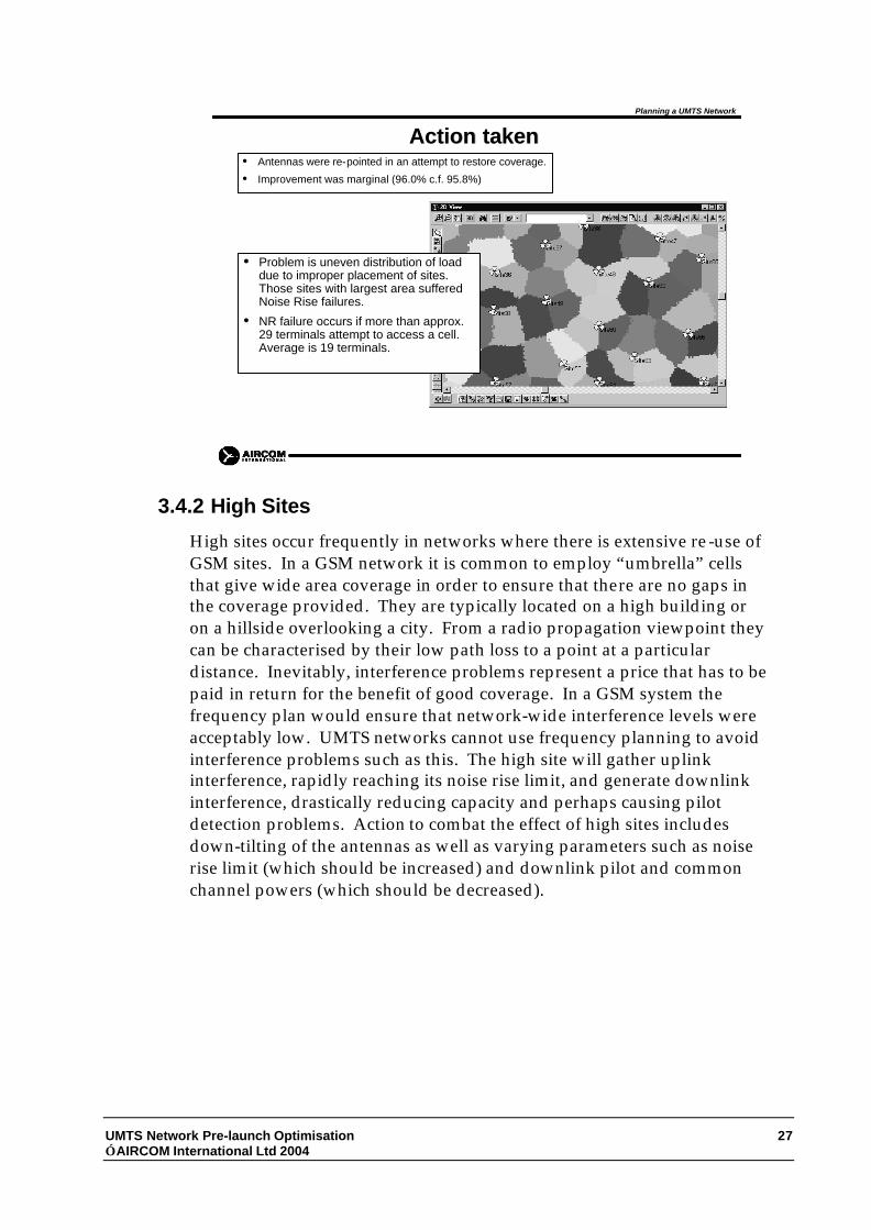
Action takenAction taken• Antennas were re-pointed in an attempt to restore coverage.
• Improvement was marginal (96.0% c.f. 95.8%)
• Problem is uneven distribution of load due to improper placement of sites. Those sites with largest area suffered Noise Rise failures.
• NR failure occurs if more than approx. 29 terminals attempt to access a cell. Average is 19 terminals.
Planning a UMTS Network
3.4.2 High Sites
High sites occur frequently in networks where there is extensive re -use of GSM sites. In a GSM network it is common to employ “umbrella” cells that give wide area coverage in order to ensure that there are no gaps in the coverage provided. They are typically located on a high building or on a hillside overlooking a city. From a radio propagation viewpoint they can be characterised by their low path loss to a point at a particular distance. Inevitably, interference problems represent a price that has to be paid in return for the benefit of good coverage. In a GSM system the frequency plan would ensure that network-wide interference levels were acceptably low. UMTS networks cannot use frequency planning to avoid interference problems such as this. The high site will gather uplink interference, rapidly reaching its noise rise limit, and generate downlink interference, drastically reducing capacity and perhaps causing pilot detection problems. Action to combat the effect of high sites includes down-tilting of the antennas as well as varying parameters such as noise rise limit (which should be increased) and downlink pilot and common channel powers (which should be decreased).

UMTS Network Pre-launch Optimisation 28 AIRCOM International Ltd 2004
Problems caused by High SitesProblems caused by High Sites
• 15% of sites made “high sites” with a path loss 10 dB less than that of “normal” sites at a given range.
Planning a UMTS Network
Problems caused by High SitesProblems caused by High Sites
• Uneven loading causes disastrous results.
• Coverage probability reduced from 98.7% to 78.6%.
Planning a UMTS Network

UMTS Network Pre-launch Optimisation 29 AIRCOM International Ltd 2004
Problems caused by High SitesProblems caused by High Sites
• Probability of NR failure very high in high site area.
• FRE for high site ~ 48% (63% average)
• Throughput for high site ~ 26 E (18 E average)
Planning a UMTS Network
Action takenAction taken
• Excess coverage area reduced by down-tilting the antennas of the high-sites.
• Result:
• Coverage probability increased to 95.1% (c.f. 78% before down-tilting and 98.7% with “perfect” sites).
Planning a UMTS Network

UMTS Network Pre-launch Optimisation 30 AIRCOM International Ltd 2004
Alternative ActionAlternative Action
• Instead of down-tilting, reduce pilot power of high sites by 10 dB to equalise service areas.
• Result:
• Problem made worse! This is because terminals still caused Noise Rise even though they were not connected. Reduction of High Site service area causes an increase in Mobile Tx
power hence aggravating the problem.
Pilot Power Equal
Mobile Connects to High Site
Pilot Power scaled to equalise service areas.
Mobile Connects to Low Site - Tx Power increased
Planning a UMTS Network
Alternative ActionAlternative Action• Increased NR Limit of High Site by 10 dB
• Decreased Max Tx power, Common Chan power and Pilot power by 10 dB.
• Result:
• A dramatic improvement. Performance of network indistinguishable from ideal case.
• High NR experienced by High Site but continued to perform satisfactorily.
• Detecting the existence of High Sites is crucial.
Planning a UMTS Network

UMTS Network Pre-launch Optimisation 31 AIRCOM International Ltd 2004
Spotting a High SiteSpotting a High Site
• Examining the Best Server byPilot array is informative.
• Spreading a traffic terminal andexamining traffic captured ispossibly more informative as itconsiders traffic distribution.
• Site35C: 18.0946• Site36A: 18.2301• Site36B: 19.5065• Site36C: 18.4447• Site37A: 13.9719• Site37B: 14.4915• Site37C: 18.2414• Site38A: 37.0476• Site38B: 38.7644• Site38C: 36.72• Site39A: 10.6173• Site39B: 18.9417• Site39C: 10.1203
– High Site
Planning a UMTS Network
High Sites High Sites -- a final worda final word
• There is no single definition of a high site.
• Do not think that it is “wrong” to place UMTS base stations on hilltops.
• High sites tend to gather uplink interference generated by otherusers.
• Problems occur as area becomes more heavily loaded (if the traffic is reduced from 4000 terminals to 2000 terminals, coverage is excellent even with “untreated” high sites).
• If coverage area is very lightly loaded - no problem.
Planning a UMTS Network

UMTS Network Pre-launch Optimisation 32 AIRCOM International Ltd 2004
3.5 Using More Appropriate Path Loss Models
The path loss model used so far is too simple to be realistic. More widely used models reduce to similar equations if the height of the mobile is fixed and, also, the terrain is flat. However, incorporation of the more sophisticated models is essential if terrain height variations are to be considered.
A typical “Okumura-Hata” style of equation was used to predict the path loss over a terrain that included substantial variations in height. The variation in height caused coverage gaps to appear in the shadows of the hills. These were filled by the provisioning of additional base stations such that almost 95% of the areas covered to the required level of 146 dB path loss. It was found that some of the base stations fell into the category of “high site” and caused excessive blocking. The level of blocking could be reduced by careful re-pointing of the antennas.
Incorporating more sophisticated Path Loss Incorporating more sophisticated Path Loss ModelsModels
( ) ( ) )log()log()log()log(
)log()log()log()log(log Loss
625431
654321
dhkkhkhkhkk
dhkhkhkhk(d)kk
effeffmsms
effeffmsms
+++++=
+++++=
• “Cost 231 - Hata”
• If hms is fixed then variations are only dependent on heff. Using typical default parameters:
Antenna Ht Model15 140.0 + 32.3 log(d)20 138.2 + 31.5 log(d)25 136.9 + 30.8 log(d)30 135.8 + 30.3 log(d)
Planning a UMTS Network

UMTS Network Pre-launch Optimisation 33 AIRCOM International Ltd 2004
A More Challenging TerrainA More Challenging Terrain
154 km2. Heights vary from zero to 135 m a.s.l.
Planning a UMTS Network
The ChallengeThe Challenge
• Challenge is to serve 2000 Erlangs of demand for voice service.
• Even spread of traffic across the whole area.
• 13 E/km2
• With 20 m antenna heights, initial calculation suggests 25 sites.
• Max path loss should be 146 dB, range 1.8 km.
• Peak Noise Rise will be 8.7 dB.
Planning a UMTS Network

UMTS Network Pre-launch Optimisation 34 AIRCOM International Ltd 2004
Placing the SitesPlacing the Sites
• Due to irregular outline, 31 sites were required to provide continuous coverage at a range of 1800 metres.
Planning a UMTS Network
Coverage AnalysisCoverage Analysis
• Initial site placing leads to 80% of area being covered to required level.
• UMTS simulation suggests coverage probability of 87% with failures split between uplink Eb/No and Noise Rise.
Planning a UMTS Network

UMTS Network Pre-launch Optimisation 35 AIRCOM International Ltd 2004
Increasing Percentage CoverageIncreasing Percentage Coverage
• Adding four more sites (35 in total) resulted in 94.3% coverage based on pathloss and 92% coverage probability from UMTS simulator.
• Again failures split between Eb/No and Noise Rise.
Planning a UMTS Network
Analysing Reason for Analysing Reason for EbEb/No Failures/No Failures
• Eb/No failures follow high path loss areas. If the path loss is too great the required Eb/No cannot be achieved.
Coverage Eb/No Failures
Planning a UMTS Network

UMTS Network Pre-launch Optimisation 36 AIRCOM International Ltd 2004
Analysing Reason for NR FailuresAnalysing Reason for NR Failures
• Noise Rise failures concentrated on High Sites. An example is shown.
Coverage Strongest Pilot
Planning a UMTS Network
Action taken to decrease NR failures.Action taken to decrease NR failures.
• Starting statistics: Throughput 382 kbps (approx 31 connections); 20 blocked connections due to NR.
• Action: Height reduced to 10 m; antenna down-tilted by 3 degrees.
• Result: Throughput 294 kbps; 0.65 blocked connections due to NR; no noticeable increase in failures on neighbouring cells.
Coverage
For the cell being investigated:
Planning a UMTS Network

UMTS Network Pre-launch Optimisation 37 AIRCOM International Ltd 2004
Covering an Urban Area.Covering an Urban Area.
• 2000 Erlangs over 154 km2 is not a very big density.
• New challenge is to serve 2000 Erlangs of voice service generated by users within an area of 2.36 km2.
• This Urban area is not flat (zero to 50 m a.s.l.) or regularly shaped, posing significant challenges.
Planning a UMTS Network

UMTS Network Pre-launch Optimisation 38 AIRCOM International Ltd 2004
3.6 Serving Very High Traffic Densities
In practice, it is possible to encounter traffic densities far in excess of the 13 Erlangs per km2 examined in the last simulation. Accordingly, a small (2.4 km2) urban area was investigated with a view to servicing 2000 Erlangs of voice traffic: a density of approximately 800 Erlangs per km2.
The main finding was that the “other to own” interference ratio tends to be much higher when the cells are packed closely together. Rather than the assumed value of 0.6, values of 1.5 were encountered. This reduces the capacity per cell. Lowering the antenna heights and down-tilting helped improve the situation but not to the extent where the assumed value of 0.6 was realised. Thus it seemed impossible in the first instance to service the level of traffic with the number of cells first calculated. The network provided good coverage for 1600 terminals as opposed to the required 2000 terminals. Increasing this level to 2000 would entail re-starting the dimensioning exercise assuming a more realistic value for the interference ratio (unity being a suggested value for such situations).
This is another example of a simulation tool being required to validate spreadsheet calculations.
Spreadsheet Dimensioning.Spreadsheet Dimensioning.
• Initial dimensioning exercise predicts that coverage can be achieved by 22 sites each of range 240 metres.
• Low path loss means that very high (20 dB+) Noise Rise can be tolerated.
• Cell capacity effectively become Pole Capacity.
• Coverage prediction suggests that path loss will not be a problem.
Planning a UMTS Network

UMTS Network Pre-launch Optimisation 39 AIRCOM International Ltd 2004
UMTS Simulation.UMTS Simulation.
• Only 65% Coverage Probability achieved.
• All failures due to Noise Rise.
• Estimation of Pole Capacity of a cell is erroneous.
• Cell Reports indicate very low FRE (~40%) suggesting a value for the interference ratio, i, of 1.5 (c.f. 0.6 assumed).
• Increasing FRE is crucial to increasing capacity. Coverage Probability
Planning a UMTS Network
Optimisation Procedures.Optimisation Procedures.
• Lowering antenna heights and making the downtilt as high as 10 degrees improved matters.
• Coverage probability now 86% (c.f. 65%).
• FRE still only 50%.
• Initial estimate of 32 Erlangs per cell unachievable in first instance.
• Reduce traffic to more “realistic” levels.
Coverage Probability
Planning a UMTS Network

UMTS Network Pre-launch Optimisation 40 AIRCOM International Ltd 2004
Optimisation Procedures.Optimisation Procedures.
• Reduced traffic from 2000 to 1600 terminals.
• Coverage probability increased to 96%.
• Majority of failures due to one apparent “high site” that could probably benefit from further attention.
• 25 Erlangs per cell would appear to be the limit in this situation (average load 84%).
Coverage Probability
Planning a UMTS Network
Conclusions.Conclusions.
• Spreadsheet dimensioning is an appropriate initial step.
• Planning Tool needed to form strategy; analyse coverage; spread traffic; conduct detailed analysis; perform quantitative sensitivity analyses; predict the effectiveness of optimisation techniques.
• Control of cell antenna radiation is crucial to achieving designed capacity. In particular “high sites” can dramatically reduce the capacity of a network.
• It becomes more difficult to achieve high Frequency Re-use Efficiency as cells are packed closer together.
• Problems only become apparent as system becomes heavily loaded.
Planning a UMTS Network

UMTS Network Pre-launch Optimisation 41 AIRCOM International Ltd 2004
3.7 Evaluating Simulator Results
When examining the prediction made by a simulator it is important to be clear regarding exactly what you are simulating. Essentially, a Monte Carlo style of static simulator will provide a prediction of the outcome of attempts to establish a connection to the network. Noise Rise failures generally indicate a failure to connect because of over demand. It is very useful to gain an estimate of the likelihood of a call being dropped once a connection has been established.
If the network becomes “under stress” from overloading, or capacity being reduced due to external interference, there are various load control measures that can be introduced. These include tolerating a lower Eb/No value and also reducing the bit rate provided on a particular service. Simulations of network performance with these lower quality targets should be made and evaluated.
In these circumstances the lower values of Eb/No and bit rate should result in Noise Rise failures being eradicated. The location of areas where the likelihood of failure is high should then be identified. These will generally be areas where the path loss to the best server is too high to allow the required Ec/Io and Eb/No conditions to be met. Their seriousness can be evaluated and remedial action taken.

UMTS Network Pre-launch Optimisation 42 AIRCOM International Ltd 2004
Evaluating Simulation ResultsEvaluating Simulation Results
• The simulator provides a prediction of the outcome of attempts to establish a connection to a network.
• Of special interest is the probability of a call being dropped.
• Load control in times of stress will involve reducing Eb/No and reducing bit rates. The performance of the network under such circumstances should be evaluated.
Planning a UMTS Network
Evaluating Simulation ResultsEvaluating Simulation Results
• With reduced Eb/No and bit rates (e.g. Eb/No 2 dB below target and voice bit rate reduced to 7.95 kbps), Noise Rise failures should be extremely rare (ideally zero).
• Eb/No and Ec/Io failures will probably be confined to small “problem areas” which will usually be related to high path loss.
Location of Failures
Planning a UMTS Network
3.8 Pilot Pollution
The term “pilot pollution” is used in various texts to describe a number of related yet distinct problems. Essentially, they all relate to the situation where a similar path loss exists from a mobile to many (four or more) cells. It is possible under such circumstances for the total received power to be so high that Ec/Io failures are recorded due to the high level of Io.

UMTS Network Pre-launch Optimisation 43 AIRCOM International Ltd 2004
Pilot PollutionPilot Pollution
• If a mobile experiences comparable path loss to a number of cells, problems can arise through no single cell dominating.
• Problems include: low Ec/Io; low capacity on downlink; frequent updates to membership of the active set.
Planning a UMTS Network
The value of Ec/Io at a point depends on the pilot power of the best server, Pp, the other power transmitted by the best serving cell, T1 (that will benefit from orthogonality α), the link loss to best serving cell, LL1, the transmit powers of interfering cells (T1, T2, T3 etc..) and the link loss to these interfering cells (LL2, LL3, LL4 etc.).
( )( )
++++−−
=....
33
22
111
1log100
LLT
LLT
PLLPT
LLP
IE
NP
Pc
α
dB

UMTS Network Pre-launch Optimisation 44 AIRCOM International Ltd 2004
EcEc/Io/Io
• In the above situation the pilot power would be received at a level of -97 dBm.
• Total of interference plus noise would be -89.5 dBm giving a value for Ec/Io of -7.5 dB.
Pilot Power: 33 dBm“Interference” Power: 40 dBm
Link Loss 130 dB
Noise Floor: -99dBm
Planning a UMTS Network
• The power from a neighbouring site would add to the total interference and noise power. In the above situation this total power would become -86.2 dBm and Ec/Io would be reduced to -10.8 dB
Pilot Power: 33 dBm“Interference” Power: 40 dBm
Link Loss 130 dB
Interference Power: 42 dBm
Link Loss 131 dB
EcEc/Io/Io
Planning a UMTS Network

UMTS Network Pre-launch Optimisation 45 AIRCOM International Ltd 2004
More likely is the situation arising where downlink throughput is severely limited by the interference. A quick analysis of the approximate expression for the pole capacity in the downlink direction demonstrates that the value of parameter, i, is crucial. If the cell has a similar path loss to many cells, then values of i as large as five can be encountered thus reducing the capacity possible on the downlink at those regions suffering from the interference.


UMTS Network Pre-launch Optimisation 47 AIRCOM International Ltd 2004
4 Further issues: Neighbours, Scrambling Codes, GSM co-location
4.1 Introduction The previous section dealt with planning the “physical” aspects of a UMTS network. This is necessary but not sufficient to ensure successful network operation. Configuration of the network will crucially include defining neighbour lists for each cell in the network. This list should be optimised. Put simply, the planner should be aware of the following constraints.
• If the neighbour list is too short, it may omit a significant server. This omitted cell will suffer UL interference from mobiles and, further, generate DL interference.
• If the neighbour list is too long the mobile will have to undertake a large amount of processing. Further, there is a maximum list length of 32 that a mobile can accommodate. This is a maximum even when in hand over (in which situation the neighbour list is merged). If the combined neighbour lists of the cells in the active set exceeds 32, the list will be truncated. This may result in significant potential serving cells being omitted from the list.
As part of the neighbour list optimisation process, neighbours should be prioritised. This will then ensure that any neighbours that are deleted from the list as part of a truncation process are not the most significant neighbours. Neighbours can be either:

UMTS Network Pre-launch Optimisation 48 AIRCOM International Ltd 2004
• Cells sharing the same UMTS carrier frequency (allowing soft or softer hand over to occur).
• Cells using separate UMTS carrier frequencies (for which hand over will always be “hard”).
• Other Radio Access Technologies (necessitating an “Inter Radio Access Technology” (IRAT) hand over).
4.2 Producing and Prioritising the Neighbour List
4.2.1 Intra-frequency carriers
Getting the intra-frequency neighbour list “right” is critical to network success as a cell that cannot join the active set could become a significant interferer. Neighbours will be able to join an active set when a cell for which it is defined as a neighbour is already a member of the active set. If the neighbour uses the same UMTS carrier frequency, the neighbour will be able to form soft or softer hand over with this cell. Softer hand over refers to the situation when both cells are on the same site. Particularly if the number of cells is limited to three, co-located sites will almost invariably be neighbours of each other. The remainder of this section deals with the problem of identifying appropriate neighbours. For a cell to be declared as a neighbour it should be possible for a hand over to occur between it and the serving cell. One criterion is that the path loss should be small enough from the edge of the serving cell to allow a connection to be sustained. For soft hand over to be entered into, the pilot strengths (and, usually therefore, the path losses) must be within a predefined small window known as the SHO margin (the full SHO process is more complicated than this but this approximation suits the purpose of deciding on a neighbour list). The difference between the path loss will also indicate the degree of mutual interference between cells. One useful indicator of the suitability of a cell as a neighbour is the percentage of the coverage area of the best server for which a potential neighbour has a pilot strength within the SHO margin.
Using this criterion, a planning tool can be used to create a neighbour list. It must be borne in mind that the propagation model within the planning tool will predict the pilot strengths at a pixel. Shadow fading should be considered when assessing the likely percentage of that pixel that would meet the requirement for SHO. For example, suppose the SHO margin in 3 dB and the predicted difference in pilot strengths for a pixel is 5 dB. The standard deviation of this difference in path loss will depend upon the correlation of the path loss to the two cells. It is common to assume a standard value for this standard deviation. Suppose this is taken to be 6 dB. The problem now resolves into one whereby the mean difference is 5

UMTS Network Pre-launch Optimisation 49 AIRCOM International Ltd 2004
dB, the s.d. is 6 dB and we need to determine the probability of the path length difference being less than 3 dB. This in turn becomes a classic “area of the tail of a normal distribution” question with the key parameters being the standard deviation of 6 dB and the difference between the mean and the SHO window (2 dB). Use of appropriate tables or formulas reveals that the probability is 37%. Thus SHO could be expected to be established in 37% of the pixels being investigated. A value of 37% of the area should be logged. The same process should be undertaken for all pixels for which the cell being investigated is the “best server” and a list of potential neighbours can be produced in order of significance. A judgement can then be made as to the best “cut off” line.
4.2.2 Practical Guidelines to Ncell Planning
Any planned neighbour list will have to be tuned through monitoring network activity. However, it should be possible to arrive at a sensible initial plan using a combination of planning tool, drive test measurements and “common sense”. As an initial pointer, the limits of the length of the neighbour list can be agreed. In view of the fact that the neighbour list is to be merged with that of others within any active set, it would appear sensible to limit the length of any one neighbour list to approximately 16. Conversely, it is possible to obtain a very short neighbour list from a planning tool. If a required neighbour were missing, this would cause serious network problems. A lower limit of 10 neighbours is advisable. The process initially entails producing a neighbour list with the help of a planning tool. The coverage area of a cell is examined in order to determine the other cells that would be capable of joining the active set. This is done on the basis of the predicted levels of CPICH RSCP, Ec/Io and shadow fading margin. The length of the neighbour list can be altered by changing one or more of these parameters. The planning tool will produce a list of neighbours meeting the criteria set. Further, the list can be prioritised on the basis of the area for which each potential neighbour meets the criteria.
Following the generation of the neighbour list, the planner can make a manual check to ensure that no seemingly obvious neighbours have been omitted. The original list can be altered as required. This neighbour list can then be implemented onto the network for pre-launch tests. Drive test data can be used to optimise the Ncell list, as explained in Section 7.

UMTS Network Pre-launch Optimisation 50 AIRCOM International Ltd 2004
Intra-frequency Neighbour ListsIntra-frequency Neighbour Lists
NCELLS
• Defines list of potential additions to the active set.
• Cells on the neighbour list will be examined to see ifthey meet criteria to enter soft or softer hand over withthe primary server.
• Issues:• Maximum of 32• Neighbour lists of active set merged
• Priority required to avoid “best neighbour” being removed.
Identifying Suitable NeighboursIdentifying Suitable Neighbours
NCELLS
• Planning tools,such as Enterprise 3g, will planneighbours automatically using proprietary algorithms.
• Based on mutual interference of cells.
• If a cell with a strong pilot does not join the active set itwill become a strong interferer.
• Neighbours can be inward, outward or mutual.
• Neighbours should be prioritised on the basis of theamount of interference they could cause and theprobability of them forming the necessary primary serverfor an exiting UE.
• Tools are viewed as a way of generating a “first pass”neighbour list. Manually adjusted.

UMTS Network Pre-launch Optimisation 51 AIRCOM International Ltd 2004
Identifying Suitable NeighboursIdentifying Suitable Neighbours
NCELLS
• Planning tool criteria:• Pilot RSCP: minimum value required
• Pilot Ec/Io: minimum value required
• Soft HO margin: compares pilot strength of potential neighbourwith that of best server.
• Minimum area for which above criteria are met.
• Varying the above parameters will alter the length of theNcell list.
• List will be prioritised on the basis of the area for whicheach cell meets the criteria.
Identifying Suitable NeighboursIdentifying Suitable Neighbours
NCELLS
• If manual planning is adopted we need to beconsistent.
• Maximum number? (16?)
• Minimum number? (10?)
• Adjacent cells plus other significant interferers?
• All sites within a given range?
• Eventually the list will be optimised using drive testdata.

UMTS Network Pre-launch Optimisation 52 AIRCOM International Ltd 2004
4.2.3 Inter-frequency neighbours
This list is not as critical as the intra-frequency neighbour list as the interference issue will not be as serious. However the following issues should be borne in mind:
• If a micro-cell is deployed to serve a hot spot using a separate frequency, it is possible that it will not have any intra-frequency neighbours and the inter-frequency neighbour list will then be very significant.
• Macro-cells that have a micro-cell that uses a separate frequency embedded must contain that micro-cell as a neighbour. The percentage of the macro-cell area served by the micro-cell may not be large. This should be considered when deciding the criterion for admission to a neighbour list.
The criteria will not be based on the difference between the pilot strengths of the two cells but, rather, on the ability of the potential neighbour cell to provide a connection. This is usually assessed using Ec/Io as an indicator. The effect of cell loading on this parameter must be considered. For example, if –15 dB is taken as a threshold level, this is a value appropriate for cases when the network is heavily loaded. Further, the attenuation afforded by filters (typically 33 dB) must be considered when computing the effective value of Io. A final point is that, in the initial stages of UMTS rollout, it is likely that only a single carrier will be deployed.
4.2.4 Inter-Technology Neighbours.
At the initial rollout stage, IRAT hand over is expected to occur frequently. Typically, this will be from UMTS to GSM and vice versa. It should be noted that this would involve modifying the neighbour lists of existing 2G cells. IRAT hand over is most crucial at the edge of the UMTS coverage area. Optimising the neighbour list is important. The main criterion is that the neighbour should be able to sustain a connection rather than any monitoring of the difference between signal strengths from the 2G and 3G cells (as is the case with UMTS intra-frequency hand over).
4.2.4.1 UMTS to GSM Hand Over
Assuming that the GSM network is already established and that interference within this network is at acceptable levels (i.e. that the GSM network does not drop calls due to intra-network interference), this becomes a matter of assessing the signal strength from a potential GSM neighbour. The threshold level for this would depend on the environment. For example, in the open a level of –97 dBm may be

UMTS Network Pre-launch Optimisation 53 AIRCOM International Ltd 2004
appropriate but, if indoor coverage is required in the area in question, -82 dBm should be required.
If a planning tool is used to perform the initial neighbour planning, an initial step should be to identify the GSM cells that provide coverage over a significant percentage of the UMTS cell. Once these GSM cells have been identified, the decision on the neighbour list will be further influenced by whether the IRAT hand over will be implemented for coverage or capacity reasons. Initially, it may be sufficient to hand over to GSM only when UMTS coverage ceases. Therefore, a further level of the decision making process is required. This decision can be based on the pilot level at the edge of the area for which a cell is the best server. If this level is high, then an alternative UMTS cell will be available for hand over and no GSM neighbours will be required. If the level is low, then hand over to a GSM network may be required.
One major issue is that the cell density of the GSM network may be much greater than that of the UMTS network. Simply looking at GSM carriers that provide significant signal strength over a certain percentage of the coverage area of a UMTS cell could lead to a very long neighbour list being generated. The area of the cell that we need to concentrate on is that where coverage from the best serving UMTS cell is judged to be poor. Note that the maximum number of neighbours that can be analysed by any UE applies to when in soft hand over and, further, includes any inter-frequency and IRAT neighbours. An IRAT neighbour list utilising a planning tool should offer the possibility of considering only those areas where UMTS pilot strength is below a certain level.
Further issues that have to be considered include the type of service for which hand over is possible. For example, it should be possible to hand over a voice call to a GSM network but whether a video telephony call will revert to voice only in a GSM area is another matter. Further, the data rates offered to a GPRS service in each network should be defined.
4.2.4.2 GSM to UMTS Hand Over
An active call will not hand over from GSM to UMTS. Once it has conducted a UMTS to GSM hand over, the call will remain on the GSM network until termination. Handover (or re-selection onto the UMTS network) will occur only in idle mode. If the GSM network is mature, its coverage range will exceed that of the embryonic UMTS network and hand over from GSM to UMTS will not be strictly necessary. However, the UMTS network is there to provide enhanced services and additional capacity and hand over in this direction should be possible Therefore, each GSM cell could have UMTS cells in its neighbour list. Hand over to a UMTS cell should be a priority for a suitably enabled UE. The planning of a GSM to UMTS list should be prepared in a similar manner to list for hand overs in the other direction. This would involve identifying the area

UMTS Network Pre-launch Optimisation 54 AIRCOM International Ltd 2004
for which a GSM cell is the best server on the GSM network and assessing the potential of UMTS cells as neighbours. This would be based on a criterion such as the percentage of the area for which the UMTS pilot strength was above, say, -95 dBm.
Inter Radio Access Technology (IRAT)Inter Radio Access Technology (IRAT)Hand OverHand Over
IRAT
• Customers transferring to 3g should:• gain access to video telephony services
• benefit from higher data rates for GPRS and HSCSD
• experience a service “at least as good as GSM” for voiceservices
• Satisfying this last requirement will necessitatesuccessful IRAT hand overs occurring.
Inter Radio Access Technology (IRAT)Inter Radio Access Technology (IRAT)Hand OverHand Over
IRAT
• Active UE will hand over to GSM when Ec/Nothresholds are met.
• Ec/No should be logged.
Ec/No
time
Enter compressed mode
Perform Hand Over

UMTS Network Pre-launch Optimisation 55 AIRCOM International Ltd 2004
Inter Radio Access Technology (IRAT)Inter Radio Access Technology (IRAT)Hand OverHand Over
IRAT
• Active UE will not hand back to UMTS network.
• Idle UE can undergo reselection in both directions.
Inter Radio Access Technology (IRAT)Inter Radio Access Technology (IRAT)Hand OverHand Over
IRAT
• The neighbour list of UMTS cells should include GSMcells.
• The neighbour listincludes:
• The co-located GSM cell
• Neighbours of this cell

UMTS Network Pre-launch Optimisation 56 AIRCOM International Ltd 2004
4.3 Scrambling Code Planning A cell must be allocated 1 of a possible 512 scrambling codes. The scrambling code is the pilot channel. The mobile uses this to synchronise to so that it can demodulate traffic channels and common control channels. It is clear that satisfactory network operation requires that a mobile receive a particular pilot channel from a clearly identifiable cell. If it receives the same pilot channel from two or more cells, confusion will result. The 512 codes are divided into 64 groups with 8 codes in each group. There are advantages if the number of codes per group is restricted or if the number of groups used is restricted. These advantages are in the form of:
• Handover time/success
• Mobile battery life
Often all cells in a cluster will be allocated the same code number (each cell would then have a different group). Adjacent clusters would be allocated a different code number. This provides a straightforward way of ensuring that identical codes do not interfere with each other. It may indeed be possible to allocated scrambling codes to the entire network on the basis of using the same code number throughout. This would then provide a re-use factor of 64, which should be sufficient while the site density is not great. An alternative strategy is to allocate cells on a particular site three codes from the same group (e.g. 0, 1 and 2). Different sites would then be allocated different code groups (from 0 to 63).
Speed of acquisition depends on the match between the allocations of codes in the network and the search strategy of the mobile. This is specific to a manufacturer and it is therefore not possible to generalise regarding an optimum planning strategy. Code planning for UMTS networks is not as influential on performance as frequency planning is for GSM networks.

UMTS Network Pre-launch Optimisation 57 AIRCOM International Ltd 2004
5 Assessing a Plan
The nominal plan will exist as a database that can be viewed and manipulated using a planning tool. It is important to be aware of initial criteria that should be met regarding
• Coverage
• Capacity
• Interference
Network capacity will be limited by the number of sites and the sophistication of the technology employed (e.g. is diversity implemented). For a given configuration, capacity can be thought of as intimately related to interference and therefore meeting interference criteria will lead to the capacity being at a near optimum for the infrastructure employed.
5.1 Coverage Coverage is thought of as uplink limited. For any environment a maximum link loss can be determined for a given service. The question “for which service shall we plan coverage?” is important. There is a general expectation that UMTS should provide more than voice services as standard and a 64 kbit/s video-telephone is often selected as a “benchmark” service. A typical link budget for this is given below. Note that the strategy is to determine the maximum link loss that can be tolerated on the uplink and then use downlink parameters to indicate the coverage area on a planning tool.

UMTS Network Pre-launch Optimisation 58 AIRCOM International Ltd 2004
UL Budget for CS 64 kbit/skTB -108.1 dBmNoise Figure of Receiver 3 dBRequired Eb/No 4 dBProcessing Gain 17.8 dBNoise Rise Margin 4 dB
Minimum Receive Power -114.9 dBm
UE Tx Power 21 dBm
Maximum Link Loss 135.9 dB
Pilot Tx Power 33 dBmReceive Pilot Strength at UE -102.9 dBm
Margins:Power Control Margin 1 dBShadow Fading Margin (95% at indoor s.d. of 7 dB) 7 dBPenetration Loss (Urban bldg) 15 dBSHO gain at cell edge 4 dB
Target Pilot Strength -83.9 dBm
The conclusion from the above link budget is that the planning tool should predict a street level pilot strength of better than –84 dBm at the cell edge in order to give an indoor coverage probability of 95% in an urban area. In other areas, the target pilot strength would be different to account for differences in: • Shadow Fading Margin: if the s.d. is higher then the shadow fade
margin must be increased. Whereas a margin of 7 dB is required if the s.d. is 7 dB, 13 dB margin is required if the s.d is 11 dB (a typical figure for some indoor environments).
• Building Penetration Loss: The above budget includes 15 dB as an allowance for building penetration loss. This may reduce in suburban areas and increase in dense urban areas. In areas where coverage is of a highway, then the budget can be modified to allow for in-car, rather than in-building coverage.
Typical adjustments relative to the target pilot for urban areas are given below:
Environment Adjustment
Dense Urban +5 dB
Suburban -5 dB
Highway -10 dB
Open -15 dB

UMTS Network Pre-launch Optimisation 59 AIRCOM International Ltd 2004
Thus, in assessing a plan table below provides typical coverage criteria.
Environment Requirement
Dense Urban 95% of pixels covered to a pilot strength of >-79 dBm
Urban 95% of pixels covered to a pilot strength of >-84 dBm
Suburban 95% of pixels covered to a pilot strength of >-89 dBm
Highway 95% of pixels covered to a pilot strength of >-94 dBm
Open 95% of pixels covered to a pilot strength of >-99 dBm
Note that this is a methodology for assessing a plan produced using a planning tool. It does not refer to levels of pilot strength that should be measured over a required coverage area. Note also that the predictions are for street level and that building penetration loss has been accounted for by allowing an appropriate margin.
5.1.1 The effect of MHAs on the coverage targets
By using downlink field strength as an indicator of uplink coverage we are making the assumption that the link loss will be the same in both directions. The use of a MHA renders this assumption incorrect. The difference between the link loss in the two directions will be mostly influenced by the feeder loss. The MHA can be thought of as effectively “cancelling” the feeder loss and the SNR at the top of the mast is the same as that at the receiver. However, the feeder loss has a direct influence on the downlink pilot strength. It is a common practice to use high quality feeder where longer lengths are required in order to make feeder loss consistent across the network. 3 dB is a typical nominal figure. This would reduce the target levels for pilot strength by 3 dB whilst maintaining uplink coverage. In a planning tool there is a choice in using the tool to assess uplink coverage in cases where a MHA is used:
1. Set feeder loss to 0 dB and use the figures given above
2. Set feeder loss to 3 dB and adjust the figures accordingly
The second choice is probably more prudent as it will lead to a more valid simulation of the downlink performance in general. It is, of course, possible to simulate each site “as it is” (that is, enter measured feeder losses for every cell) but this would entail setting different coverage targets for each cell, making a “first pass” assessment very tedious.
Examining the above approach makes it clear that planning is made easier if an “all or nothing” decision is made regarding the adoption of MHAs in a network. A consistent approach, at least across a particular environment, will make assessing a plan much easier.

UMTS Network Pre-launch Optimisation 60 AIRCOM International Ltd 2004
Summarising, it is recommended that, for uplink coverage assessments, a standard feeder loss is used when MHAs are implemented. If 3 dB is selected as a suitable figure then the following criteria would be suitable.
Environment Requirement (MHA implemented; 3 dB feeder loss)
Dense Urban 95% of pixels covered to a pilot strength of >-82 dBm
Urban 95% of pixels covered to a pilot strength of >-87 dBm
Suburban 95% of pixels covered to a pilot strength of >-92 dBm
Highway 95% of pixels covered to a pilot strength of >-97 dBm
Open 95% of pixels covered to a pilot strength of >-102 dBm
A final thought is that the above arguments would not be necessary if a policy of declaring downlink transmit powers at the masthead rather than at the “rack output” was adopted. This automatically accounts for feeder loss. Thus the table above can be considered appropriate if the pilot power at the masthead is +30 dBm (as opposed to +33 dBm at the rack).
5.1.2 Summarising
The process may be summarised as follows
1. Determine the maximum uplink loss that can be tolerated for the existing network parameters
2. Calculate the downlink pilot power that would be measured at this level of loss
3. Add margins to consider
a) Power control
b) Shadow fading (LNF): e.g. 7 dB to provide a 95% area probability if the s.d. of LNF is 7 dB.
c) Soft Handover Gain in uplink at cell edge.
d) Building Penetration loss
Note:
1. Different clutter categories will require different margins
2. LNF margin is there is restore probability from 50% point location probability within a pixel to 95% area over the cell coverage area (approx 82% point location probability at cell edge). Therefore prediction to the level indicated in the above table should be for the mean within any pixel.

UMTS Network Pre-launch Optimisation 61 AIRCOM International Ltd 2004
5.2 Interference
5.2.1 Pilot SIR and Ec/No
When a plan is being assessed with a view to a pre-launch optimisation programme being undertaken, the main issue is to ensure that the pilot SIR (calculated by considering the effect of orthogonality on “own cell” interference and not including the pilot itself in the total “interference” level) is sufficient to allow the UE to synchronise to the downlink. The exact value required varies from UE to UE but a typical value of –15 dB is used for most planning purposes.
We now have to consider the need for a margin for pilot SIR. A few issues need to be considered:
If the coverage criteria are met, the network will be “interference limited” rather than “thermal noise limited”. This means that variations in the interference level can be expected to be somewhat correlated with variations in the wanted signal level (almost 100% correlation when the interference is “own cell”). It is therefore not necessary to adopt a LNF margin as high as 7 dB. Allowing a 5 dB margin is expected to prove a cautious approach.
Pilot SIR is expected to be lowest near the cell edge. At these points the UE would be likely to enter SHO. This has the effect that an interferer becomes “wanted”. Nevertheless, all pilots involved need to be received with sufficient strength to allow the UE to synchronise.
5.2.2 Predicting levels on a heavily loaded network
The level of pilot SIR will reduce as the total downlink power increases. There is no purpose in configuring RBSs with a power capability of 43 dBm if this is not going to be used. It is therefore important that pilot SIR is predicted when the network is heavily loaded.
When assessing pilot SIR, it is necessary to artificially load the downlink of the network (by, for example, allocating a lot of power to a common channel). Then, 95% of the area should be provisioned such that the pilot SIR is better than –10 dB. An alternative measure is Ec/No where “No” includes the pilot itself and ignores any orthogonality effect. If an orthogonality value of 0.6 is assumed, then the value of own cell interference is reduced by 10 log (1-0.6) = 4 dB. Thus 42 dBm of “interference” has an effective value of 38 dBm. If 33 dBm of this is the

UMTS Network Pre-launch Optimisation 62 AIRCOM International Ltd 2004
pilot itself then the true interference value is reduced further to 36.3 dBm, a total reduction of 4.7 dB. However, the most serious situations are those where the downlink receive power is made up of almost equal contributions from three cells. In this case the reduction in total interference power is only 1.2 dB. Thus a predicted Ec/No value of better than –11 dB in a heavily loaded network would be an appropriate target to achieve with a planning tool.
Summarising requirements for assessing interference levels. Where coverage is achieved to the levels described in the previous section:
1. Simulate a heavy load on the network (e.g. +42 dBm total Tx power from each cell)
2. Pilot SIR should be >-10 dB
3. Pilot Ec/No should be >-11 dB
5.2.3 Expected predictions on a lightly loaded network
If the prediction is made without artificially loading the network this will lead to a higher level of Ec/No being predicted. The difference this makes depends on the relative levels of the sources of “No”, namely thermal noise and intra-network interference. This, in turn, is very location dependent. If “No” is mainly thermal noise then the difference will be small. In most situations in a practical network, “No” is expected to be dominated by own-network interference. In this case the difference made when the level of loading is changed depends upon the levels of the common channels, in particular:
• The Pilot (P-CPICH);
• The Synchronisation Channels (P-SCH and S-SCH);
• The Common Control Physical Channels (P-CCPCH and S-CCPCH);
• The Paging and Acquisition Indicator Channels (PICH and AICH).
As a first approximation, the power allocated to the pilot is approximately half of the total power allocated to common channels. If Ec/No is predicted on a quiet network then the level of “No” in an area of high interference should drop by approximately 6 dB compared with when the network was heavily loaded (if cell power reduces from 42 dBm to 36 dBm). Thus, in a quiet network, values for Ec/No of greater than –5 dB should be predicted throughout the portion of the coverage area where the network is “interference limited”.
UMTS Network Pre-launch Optimisation 63 AIRCOM International Ltd 2004
An appropriate definition of “interference limited” areas is “those areas where No is 10 dB above thermal noise level when the network is heavily loaded”. If thermal noise is assumed to be –100 dBm and a heavily loaded network is transmitting a total power 10 dB above that of pilot, then a pilot level of >-100 dBm will represent the extent of the “interference limited” area. As the lowest level of coverage is a planned pilot level of –102 dBm, the entire area for which coverage is planned can fairly be regarded as interference limited on the downlink.
5.3 High Data Rate services The above guidelines have been derived by making the 64 kbit/s CS service our “benchmark”. This is assumed to be a symmetrical service and the downlink pilot strength has been used to indicate where there should be uplink coverage. It is possible that operators will wish to offer higher data rate services (e.g. 384 kbit/s), possibly in the downlink only. Ec/Io values provide a valuable indicator of the power required to deliver a service (defined by bit rate and Eb/No). The amount of power required to deliver a particular service is affected by external interference. Ec/Io levels, knowing the pilot and common channel powers on a cell, provide an estimate of the levels of interference. If a limit on the amount of power available to a single connection were imposed, that would restrict the area for which this data rate was achievable.
The following equations lead to a method of identifying areas where a particular service can be delivered. SIR = Eb/No – Processing Gain (dB)
For the remainder of the analysis values such as power are in milliwatts (rather than dBm) and ratios are not expressed in dB.
( ) ( )
−+−−=
bearertotal
totalbearertotal
bearer
PPPiPP
PSIR
α1 (1)
+−
=
other
totalother
bearer
PPiP
PSIR
α1 (2)
where bearertotalother PPP −= It is clear that the parameter, i , affects the power requirement. Ec/Io is used as a method of estimating the value of i .

UMTS Network Pre-launch Optimisation 64 AIRCOM International Ltd 2004
( )
1
1
0
0
−×
=
+=
IEP
Pi
iPP
IE
cTOT
PILOT
TOT
PILOTc
(3)
where PILOTP is the transmitted pilot power; TOTP is the total power transmitted for the Ec/Io tests (e.g. if the network was quiet, 36 dBm would be a suitable estimate). Substituting for i in (2) gives:
( )
( )
pilot
total
pilot
bearer
pilot
other
other
total
pilot
bearer
c
cother
pilot
other
totalother
bearer
PxP
xPP
SIRPP
PP
PP
SIRPP
IE
IEP
P
PP
P
PSIR
max
max
0
0
1
11
1
−++=
−++=
+−−
=
α
α
α
(4)
where maxPPx other= This allows the level of Ec/Io to be determined if the other parameters are known, or assumed. In particular it allows the variation in required Ec/Io as a function of x to be predicted if the other parameters are fixed.
The graph below shows this variation for the following parameters:
dBm 33dB 5-
0.6dBm 43
dBm 39
max
==
==
=
pilot
bearer
PSIR
P
P
α
Note that, as the bearer is 39 dBm and the maximum power is 43 dBm, the highest value of x (representing full load) is 0.6. In other words, the 39 dBm pilot power alone represents a load of 40%.

UMTS Network Pre-launch Optimisation 65 AIRCOM International Ltd 2004
Ec/Io for 384 kbps 5 dB Eb/No bearer
-13.2
-13
-12.8
-12.6
-12.4
-12.20.5 0.6 0.7 0.8 0.9 1
Loading Factor
Ec/
Io (
dB
)Ec/Io required vsloading
If the above chart is examined, it is seen that it suggests 39 dBm is sufficient to support a 384 kbps bearer with an Eb/No of 5 dB in an area where Ec/Io on a heavily loaded (loading factor = 1) network is recorded as –13 dB and cells are transmitting a total power of 43 dBm. The logic of this particular instance is now explained. The value of Ec/Io refers to the situation where all cells are transmitting 33 dBm pilot powers and approximately 42.5 dBm of other common channel powers. A value of Ec/Io of –13 dB indicates that the pilot represents only 5% of the power received. A further 45% will come from the own cell interference. The remaining 50% is external interference. Hence “other cell” power equals “own cell” power and i equals 1.0. If the bearer is at a level of 39 dBm and the cell is transmitting a total of 43 dBm then “own cell interference” is represented by an equivalent transmit power of 40.8 dBm. Orthogonality will reduce this to 36.8 dBm. As i equals 1.0, an effective interference power of 43.0 dBm will be received. 43.0 dBm added to 36.8 dBm gives a total of 44.0 dBm. Hence the SIR will be –5 dB which, when the processing gain of 10 dB is considered, agrees with the Eb/No value of +5 dB.

UMTS Network Pre-launch Optimisation 66 AIRCOM International Ltd 2004
Assessing a PlanAssessing a Plan
Assessing a Plan
• As an optimisation engineer, you may well be presented with someoneelse’s plan as a starting point.
• It is important that you understand the thinking behind the plan and that weoptimise “to the plan”.
• Otherwise time could be spent inefficiently, perhaps “attempting theimpossible” or at least attempting to do something that has previously beenregarded as unnecessary.
• Plans are assessed on the basis of• Coverage• Capacity
• Interference
• Capacity will be influenced by the number of sites and, for a giveninfrastructure, optimising capacity can be related directly to optimisinginterference levels.
Pilot SIR, Ec/Pilot SIR, Ec/IoIo, Ec/No, Ec/No
Assessing a Plan
• Ec/Io is used interchangeably with Ec/No.• No consideration is given to the effect of orthogonality
• The pilot itself is included with Io (or No).
• Pilot SIR considers orthogonality and pilot power is not included asinterference power.
•Pilot 33 dBm
•Total Power 43 dBm•Orthogonality = 0.6
•Ec/Io = Ec/No = 33 - 43 = -10 dB
•Non pilot power = 42.5 dBm•Orthogonality effect = 10log(1-0.6)= -4 dB
•Pilot SIR = 33 - 38.5 = -5.5 dB

UMTS Network Pre-launch Optimisation 67 AIRCOM International Ltd 2004
CoverageCoverage
Assessing a Plan
• In the first instance, coverage is assumed to be uplink limited.
• We need a benchmark service: e.g. 64 kbit/s CS (videotelephony).
• In the plan, pilot strength (a downlink parameter) is used to assess uplinkcoverage.
•Pilot strength indicates path loss.
•Uplink coverage is limited by path loss.
CoverageCoverage
Assessing a Plan
Uplink
Transmitter Power 250.00 mW21.00 dBm
Tx Antenna Gain 0.00 dBiBody Loss 2.00 dBEIRP including losses 19.00 dBm
Thermal Noise Density -174.00 dBmReceiver Noise Figure 3.00 dB Receiver Noise Density -171.00 dBm/HzReceiver Noise Power -105.16 dBm Loading factor 60%Interference Margin (NR) 3.98 dB
• Esc and Double-click on spreadsheet to activate

UMTS Network Pre-launch Optimisation 68 AIRCOM International Ltd 2004
General ConclusionsGeneral Conclusions
Assessing a Plan
• Benchmark service 64 kbit/s, 4 dB Eb/No
• Urban Environment: 15 dB penetration loss
• MHA as standard
• 30 dBm pilot power at masthead (33 dBm at rack output).• LNF margin 7 dB
• SHO gain at cell edge, 4 dB
• Power Control Margin 1 dB
• UE Tx Power +21 dBm
• UL coverage is expected where DL pilot is better than -87 dBm.
•Note: -87 dBm is “local mean” level (the “planned” level) at street level.
•This is to ensure that 95% of points in the coverage area have pilot better than -94 dBm
The effect of The effect of MHAsMHAs
Assessing a Plan
• MHA helps the uplink but not the downlink.
• If the DL is used as an indicator, the MHA must be considered.
• Effectively, MHA allows feeder loss to be ignored.
• Feeder loss cannot be ignored on the UL.
• If an estimate of 3 dB feeder loss is adopted then pilot requirements are 3
dB less with an MHA than they would be if the MHA was removed.
• Presence of MHA means that the masthead becomes the point of
consideration, rather than the rack output: once the UL signal arrives at the
masthead, the MHA will “look after it” from there.

UMTS Network Pre-launch Optimisation 69 AIRCOM International Ltd 2004
Requirements for differentRequirements for differentenvironmentsenvironments
Assessing a Plan
• Different environments will require different offsets in the link budget. The
following table represents a typical variety of pilot strength requirements as
output by a planning tool.
Environment Requirement (MHA implemented; 3 dB feeder loss)
Dense Urban 95% of pixels covered to a pilot strength of >-82 dBm
Urban 95% of pixels covered to a pilot strength of >-87 dBm
Suburban 95% of pixels covered to a pilot strength of >-92 dBm
Highway 95% of pixels covered to a pilot strength of >-97 dBm
Open 95% of pixels covered to a pilot strength of >-102 dBm
•Note: 95% of pixel requirement simply acknowledges that nothing is perfect
•It is not a “coverage probability” simply a requirement for the planning tool output.
The effect of UL The effect of UL Tx Tx PowerPower
Assessing a Plan
• UL budget is directly affected by the UL transmit power.
• +21 dBm is assumed in this instance.
• Network can “decide” whether to set this to +24 dBm.
• This would have implications for UE battery life.
• +21 dBm assumption is considered appropriate.

UMTS Network Pre-launch Optimisation 70 AIRCOM International Ltd 2004
Pilot SIR and Ec/NoPilot SIR and Ec/No
Assessing a Plan
• Pilot SIR is a pass/fail requirement.
• UE dependent parameter but pilot SIR > -15 dB is generally accepted.
• Issues
• Using Ec/No as an indicator (pilot SIR is not measured)
• Planning margins for Ec/No
Pilot SIR and Ec/No: marginsPilot SIR and Ec/No: margins
Assessing a Plan
• Most networks will be “interference limited” (90%+ of UE Receive power will
be signal plus interference, not thermal noise).
• Therefore, if wanted signal reduces, interference is expected to reduce as
well.
• Correlation will be very high, especially if majority of interference is “own cell”interference.
• Additionally, the network will automatically identify the strongest server as
“best”.
• A margin of 2 dB is expected to be sufficient.
• “95% of area should have pilot SIR better than -13 dB.”
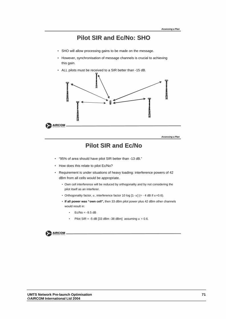
UMTS Network Pre-launch Optimisation 71 AIRCOM International Ltd 2004
Pilot SIR and Ec/No: SHOPilot SIR and Ec/No: SHO
Assessing a Plan
• SHO will allow processing gains to be made on the message.
• However, synchronisation of message channels is crucial to achievingthis gain.
• ALL pilots must be received to a SIR better than -15 dB.
Pilot SIR and Ec/NoPilot SIR and Ec/No
Assessing a Plan
• “95% of area should have pilot SIR better than -13 dB.”
• How does this relate to pilot Ec/No?
• Requirement is under situations of heavy loading: interference powers of 42
dBm from all cells would be appropriate.
• Own cell interference will be reduced by orthogonality and by not considering the
pilot itself as an interferer.
• Orthogonality factor, α, interference factor 10 log [1- α] (= - 4 dB if α=0.6).
• If all power was “own cell”, then 33 dBm pilot power plus 42 dBm other channels
would result in:
• Ec/No = -9.5 dB
• Pilot SIR = -5 dB [33 dBm -38 dBm] assuming α = 0.6.

UMTS Network Pre-launch Optimisation 72 AIRCOM International Ltd 2004
Pilot SIR and Ec/NoPilot SIR and Ec/No
Assessing a Plan
• The most serious situation is where the UE receives interference from manycells.
• Then the reduction is less.
• Suppose receive power is:
• wanted pilot 33 dBm
• own cell interference 42 dBm (reduced to effectively 38 dBm by orthogonality)
• other cell power 46 dBm (two heavily loaded interferers at similar path loss towanted cell.
• Total power received equivalent to 47.6 dBm transmit power (42 dBm + 33dBm + 46 dBm)
• Ec/No -14.6 dB
• Total effective interference power equivalent to (46 dBm + 38 dBm =) 46.1dBm.
• Pilot SIR = -13.1 dB (a difference of only 1.5 dB)
Pilot SIR and Ec/NoPilot SIR and Ec/No
Assessing a Plan
• If a pilot SIR of better than -13 dB is required, a pilot Ec/No (inconditions of heavy loading) of better than -15 dB would be anappropriate target.
Summary:•perform a prediction with cellsheavily loaded (e.g. +43 dBm Txpower per cell)•pilot Ec/No should be >-15 dB.

UMTS Network Pre-launch Optimisation 73 AIRCOM International Ltd 2004
Pilot SIR and Ec/No: lightly loadedPilot SIR and Ec/No: lightly loadednetworksnetworks
Assessing a Plan
• The level of loading will have a great effect on Ec/No levels.
•Pilot
•synchronisation•Common control
•Paging and AICH
•Traffic
• In a cell with a maximum powercapability of +43 dBm, typically 33dBm would be pilot and 33 dBmwould be other common channelpowers.
• Variation in transmitted power is from36 dBm to 43 dBm a variation of 7dB. Ec/No will vary likewise, by 7dB.
Pilot SIR and Ec/No: lightly loadedPilot SIR and Ec/No: lightly loadednetworksnetworks
Assessing a Plan
• If simulation is done for a lightly loaded network (total transmitpower 3 dB above pilot):
• 95% of area for which coverage is provided should have apredicted Ec/No greater than -8 dB.
Summary:• perform a prediction with cellslightly loaded (common channelsonly)• pilot Ec/No should be >-8 dB.

UMTS Network Pre-launch Optimisation 74 AIRCOM International Ltd 2004
High Data Rate ServicesHigh Data Rate Services
Assessing a Plan
• So far coverage predictions have been related to:
• Using DL pilot as an indicator of UL coverage
• 64 kbps, 6 dB Eb/No CS is benchmark service
• Service is symmetrical
• One additional service to be offered is likely to be 384 kbps PSin downlink only.
• Eb/No required is predicted to be 6 dB (BLER?)
• Processing Gain of 10 dB leads to a wideband SIR of -4 dB as arequirement.
High Data Rate ServicesHigh Data Rate Services
Assessing a Plan
( ) ( )
−+−−=
bearertotal
totalbearertotal
bearer
PPPiPP
PSIRα1
• An iterative process is required for solution
• Setting Pbearer to the maximum on RHS is a sensibleapproximation.
( )
1
1
0
0
−×
=
+=
IEP
Pi
iPP
IE
cTOT
PILOT
TOT
PILOTc
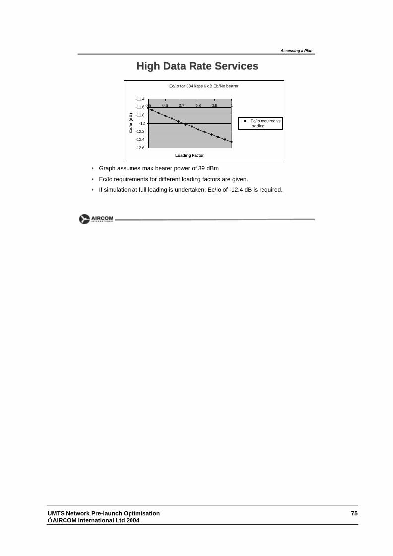
UMTS Network Pre-launch Optimisation 75 AIRCOM International Ltd 2004
High Data Rate ServicesHigh Data Rate Services
Assessing a Plan
• Graph assumes max bearer power of 39 dBm
• Ec/Io requirements for different loading factors are given.
• If simulation at full loading is undertaken, Ec/Io of -12.4 dB is required.
Ec/Io for 384 kbps 6 dB Eb/No bearer
-12.6
-12.4
-12.2
-12
-11.8
-11.6
-11.4
0.5 0.6 0.7 0.8 0.9 1
Loading Factor
Ec/
Io (d
B)
Ec/Io required vsloading


UMTS Network Pre-launch Optimisation 77 AIRCOM International Ltd 2004
6 Drive Test Analysis
6.1 Introduction When the network was planned and assessed, certain guidelines were adopted regarding the levels of pilot strength, pilot SIR and pilot Ec/No that should be regarded as key parameters for planning purposes. The previous section gives details of recommended planning levels including appropriate margins. These have been designed so that the resulting radio coverage and interference levels following the network build phase will be acceptable. It must be remembered, however, that the drive test will be carried out at street level with an external antenna and that the requirement in many areas is that the coverage should extend to indoors. Measured results should correspond to the plan. For an urban environment, the planned levels were for a pilot level of –87 dBm. This is the mean level at the edge of the cell. This level was arrived at by building in a margin that should lead to the pilot being greater than –94 dBm in 95% of locations. The reasoning was that, if the pilot is at a strength of –94 dBm at street level, 21 dBm of transmit power on the uplink will deliver the required SNR at the mast head allowing for a building penetration loss of 15 dB.
However, the statistics for cells serving urban areas as a whole should be that the pilot strength is measured as better than –94 dBm for 95% of locations.
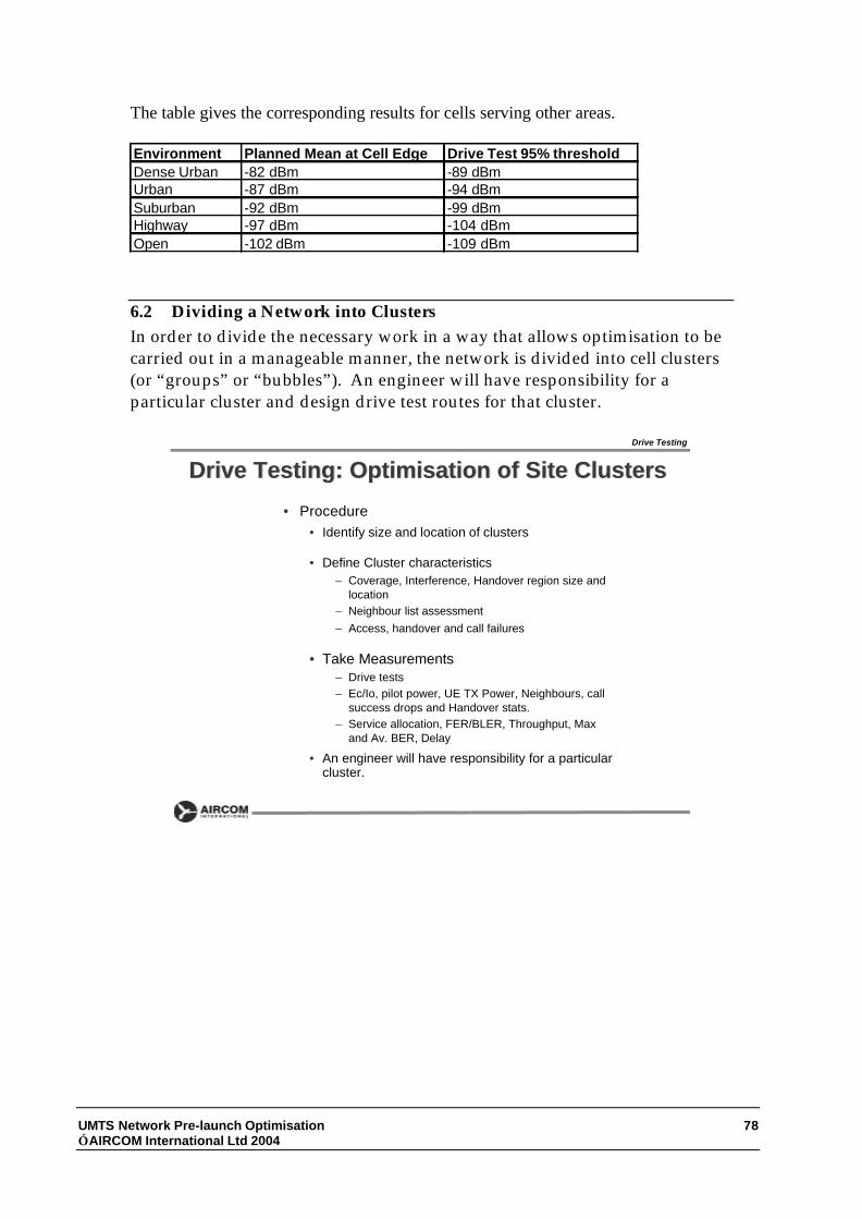
UMTS Network Pre-launch Optimisation 78 AIRCOM International Ltd 2004
The table gives the corresponding results for cells serving other areas. Environment Planned Mean at Cell Edge Drive Test 95% thresholdDense Urban -82 dBm -89 dBmUrban -87 dBm -94 dBmSuburban -92 dBm -99 dBmHighway -97 dBm -104 dBmOpen -102 dBm -109 dBm
6.2 Dividing a Network into Clusters In order to divide the necessary work in a way that allows optimisation to be carried out in a manageable manner, the network is divided into cell clusters (or “groups” or “bubbles”). An engineer will have responsibility for a particular cluster and design drive test routes for that cluster.
Drive Testing: Optimisation of Site ClustersDrive Testing: Optimisation of Site Clusters
• Procedure• Identify size and location of clusters
• Define Cluster characteristics– Coverage, Interference, Handover region size and
location– Neighbour list assessment– Access, handover and call failures
• Take Measurements– Drive tests– Ec/Io, pilot power, UE TX Power, Neighbours, call
success drops and Handover stats.– Service allocation, FER/BLER, Throughput, Max
and Av. BER, Delay
• An engineer will have responsibility for a particularcluster.
Drive Testing

UMTS Network Pre-launch Optimisation 79 AIRCOM International Ltd 2004
Cluster DefiningCluster Defining
• Identify Clusters of sites• Based on
• Terrain
• Traffic distribution
• Network is to be optimised in clusters
• This method provides for• Work delegation
• Progress tracking
• Minimises tool processing time
Drive Testing
Cluster DefiningCluster Defining
Network of clusters Cluster of sites Site
Site ApprovalCluster Approval
NetworkAcceptance Datafill
Eg ScramblingCodes; Node BParameters
Drive Testing

UMTS Network Pre-launch Optimisation 80 AIRCOM International Ltd 2004
Drive Test RoutesDrive Test Routes
Drive Testing
• Drive testing should be performed
on radial and circumferential routes
• Radial routes show variation
in signal quality with distance
from base station
• Circumferential routes provide
predictions for signal quality in
different directions from the basestation
• Typically, three routes should be
defined per cluster: consistency isvital.
6.3 Choosing the drive test route. The drive test route must be representative for the cell. A circular route at a constant distance from the site is not appropriate. Similarly, driving along a straight line at a constant bearing from the site will not reveal sufficient information. The route should allow a rich variety of distance and bearing variations to be included in the measurements.
6.4 Cells covering more than one environment It will often be the case that a cell’s coverage area includes more than one clutter category. This can distort the relationship between the planned mean level at the cell edge and the measured statistics. Suppose for example, a cell’s coverage area consists of mainly open areas plus a small urban area at its edge. If the urban area is almost all at the –87 dBm mean level then it can be expected that the probability of a measurement made at any point is above –94 dBm is only 83% rather than 95%. This is an inevitable result of the urban area, in this instance, being concentrated in locations where the path loss is high. This fact should be borne in mind when assessing measurement results. Of course, placing sites so that areas of high subscriber density are far away is not good planning practice.
6.5 Measured values of Ec/No. As well as measuring pilot power, Ec/No (or Ec/Io as it is sometimes referred to) is also measured. The requirement is that pilot SIR is above –15 dB in 95%

UMTS Network Pre-launch Optimisation 81 AIRCOM International Ltd 2004
of locations for which coverage is provided when the network is heavily loaded. This corresponds to a requirement for Ec/No that it should be better than approximately –16 dB for 95% of the area in conditions of heavy loading. If the network is lightly loaded then the level of No can be expected to fall by approximately 6 dB. Therefore drive tests should reveal that 95% of locations for which coverage is provided should experience an Ec/Io better than –10 dB. It should be noted that this is a minimum value to ensure successful network operation. It does not include and capacity optimisation features. In areas of high demand for downlink traffic, the better Ec/Io the higher the capacity. Thus it may be expected to find a higher requirement for Ec/Io in areas of high subscriber density.
6.6 The effect of network loading levels. The downlink of the network will, in all but the most exceptional circumstances, be interference limited. Variations in network load will impact directly on Ec/No levels. Thus, if the cell transmit power varies from 36 dBm to 43 dBm the value of Ec/Io at a particular location will vary by 9 dB. This does not mean that the network quality has reduced, just that the situation will vary with loading levels. Care must be taken to ensure that loading levels are known and targets adjusted accordingly.
Drive Test ResultsDrive Test Results
Assessing a Plan
• We plan for a mean (50%) level at the cell edge.
• This is done to achieve a 95% probability of a different level over the coveragearea as a whole.
• E.g. urban area will be planned to have a pilot power of -87 dBm at cell edge.This should translate to 95% of measurements over the cell area as a wholebeing >-94 dBm.
Environment Planned Mean at Cell Edge Drive Test 95% thresholdDense Urban -82 dBm -89 dBmUrban -87 dBm -94 dBmSuburban -92 dBm -99 dBmHighway -97 dBm -104 dBmOpen -102 dBm -109 dBm

UMTS Network Pre-launch Optimisation 82 AIRCOM International Ltd 2004
Drive Test Routes: cells coveringDrive Test Routes: cells coveringmultiple environmentsmultiple environments
Assessing a Plan
• Suppose the pink area in this
diagram is the urban area with the
other categories being open or
suburban.
• Planning would seek to ensure that
pilot at cell edge would be >-87
dBm.
• However location probability at cell
edge is a 83% probability of being>-94 dBm.
• Urban area will not produce results
of 95% >-94 dBm in this instance
• This must be borne in mind
when assessing drive test
results.
• “Good Planning” entails placing
sites close to areas of high
subscriber density.
Drive Tests: measuring Ec/Drive Tests: measuring Ec/IoIo
Assessing a Plan
• Requirement is for pilot SIR to begreater than -15 dB in 95% oflocations where coverage isacceptable, under conditions ofheavy loading.
• Ec/Io should be greater than -16 dBwhen network is heavily loaded.
• For quiet network Ec/Io should begreater than -10 dB for 95% of thearea.
• Higher values of Ec/Io will beneeded where high data rates onDL are required.

UMTS Network Pre-launch Optimisation 83 AIRCOM International Ltd 2004
Drive Tests: effect of loading on Ec/Drive Tests: effect of loading on Ec/IoIo
Assessing a Plan
• Ec/Io can vary by 7 dB with loadingconditions.
• It is vital that conditions at the timeof measuring are known (you willnot get Ec/Io>-10 dB on a heavilyloaded network).
• For pre-launch optimisation it iscommon to assume the network isquiet.
• But, if someone else is doing a loadtest while the drive test is takingplace…….
•Drive test
•Load test
6.7 Measurement Samples, Scanner Settings and Drive Test Speeds
It is generally regarded that the objective of a drive test measurement campaign is to obtain information regarding the “local mean” in a particular area. It should ignore fast fading but respond to changes due to “slow” or “shadow” fading. The diagram below show fast fading produced by more than one reflection imposed on top of a mean level that is nearly constant. The reason that we are more interested in the local mean is that: • It is this level that the path loss model attempts to predict • Mobile (UE) terminals are designed to accommodate multipath
environments.

UMTS Network Pre-launch Optimisation 84 AIRCOM International Ltd 2004
Fast fading
We can now discuss how the optimum results can be obtained using, as an example, the Anritsu scanner.
6.7.1 The Lee Sampling Criteria
Obtaining the most appropriate results depends on making the correct number of measurements at the correct intervals and averaging over an appropriate window. This topic has been studied in depth by William Lee and the results are known as the “Lee criteria”. These can be summarised as: • Measurements must be made at intervals of at least 0.8 λ. • The averaging window should be 40 λ in length • 36 samples should contribute to each “average” reading. Following on from these recommendations it is possible to describe the ideal measuring campaign as one that obtains a measurement every 1.1 λ and processes them so as to provide an average over 36 samples. At a frequency of 2142.4 MHz, that corresponds to: Measurements must be made at intervals of at least 11 cm. The averaging window should be 5.6 m in length

UMTS Network Pre-launch Optimisation 85 AIRCOM International Ltd 2004
36 samples should contribute to each “average” reading. The ideal measurement campaign would take measurements every 15 cm.
6.7.2 The Anritsu Scanner
The Anritsu Scanner will report on individual pilot signals within a live network. This involves synchronising to a particular cell in the presence of external interference and assessing the level of the pilot channel of that cell. Thus it performs a much more sophisticated task than a simple spectrum analyser would. This functionality is vital if it is to be able to report on signals from more than one cell within a network. Typical default settings would be: • Sampling period: 10 ms per channel (fixed) • Number of channels: 6 (user defined) • Averaging period: 1 second (user defined) At a speed of 50 kph this would translate to:
• One sample every 83 centimetres • 16 samples per averaging period • Averaging window corresponds to a distance of 13.8 metres. The table below gives the figures for other speeds. Speed (kph) inter-sample distance (cm) Samples per period Averaging distance (m)
20 33 16.7 5.640 67 16.7 11.160 100 16.7 16.780 133 16.7 22.2
100 167 16.7 27.8120 200 16.7 33.3
Already, something of a dilemma is emerging. If the ideal measurement campaign is taken as one that would take measurements every 15 cm and 36 samples are taken for every data point then the measurement period should be set to 500 ms and the speed of the test vehicle reduced to 10 kph. It is important that the implications of these variances are established.

UMTS Network Pre-launch Optimisation 86 AIRCOM International Ltd 2004
Inter –sample distance too large: not in itself a problem; the Lee criteria specify a minimum distance to ensure independence of samples. Samples per period. The smaller the number of samples, the larger the potential error in the average. Lee aimed for a standard deviation of 1 dB. This is appropriate for (highly accurate) carrier wave (CW) measurements. However it must be borne in mind that the accuracy with which pilot channels can be measured does not rival that of CW measurements. For example, an accuracy of ±2 dB is quoted for the CPICH measurements and ±3 dB for CPICH SIR. If only 17 samples are taken then the standard deviation will rise to 45.11736 = dB. This may well be seen as acceptable in the light of the unavoidable inaccuracies mentioned. Averaging Distance too large. The Lee Criteria specifies an averaging window of 40 wavelengths. That corresponds to 6 metres. The most appropriate value depends on the environment. It should be small enough to capture variations due to obstacles such as buildings and trees. Additionally, it must be small enough to allow detection of a reduction in signal strength due to increasing distance from the base station. If the UE is in the middle of a flat field, for example, then an averaging distance of several tens of metres may be appropriate with the value of 6 metres only being necessary when the environments becomes more complicated to describe.
Judging by the above comments, the major problem comes from the averaging distance being too large to permit users to be confident that all coverage holes will have been detected. The fact that the original criteria were derived for CW measurements makes it necessary to consider two further facts: The measurements have been made over a wide (4 MHz) bandwidth The receiver can use a Rake receiver with up to 6 fingers.
6.7.3 The Effect of Varying Averaging Distance The next requirement is to establish a required averaging window. A 45 metre route was used with measurements being made: Every 0.8λ with an averaging window of 5.6 metres (Lee criteria) Every 0.8λ with an averaging window of 11.2 metres.
The minimum level measured with the 5.6 metre window was –94.2 dBm whereas the minimum level measured with the 11.2 metre window was –93.1 dBm. Clearly the size of the window has the effect of

UMTS Network Pre-launch Optimisation 87 AIRCOM International Ltd 2004
smoothing out dips in the signal level. A more detailed experiment was conducted in 3 different environments.
Environment Vehicle speed (kph)Sample Rate (s)
Averaging Period (s)
Averaging Distance (m)
Samples per reading
Distance between samples (m)
Motorway 100 0.01 1 27.78 100.00 0.28100 0.01 0.5 13.89 50.00 0.28100 0.01 0.2 5.56 20.00 0.28100 0.06 1 27.78 16.67 1.67
Suburban 40 0.02 1 11.11 50.00 0.2240 0.02 0.5 5.56 25.00 0.2240 0.02 0.2 2.22 10.00 0.2240 0.06 1 11.11 16.67 0.67
commercial 20 0.03 1 5.56 33.33 0.1720 0.03 2 11.11 66.67 0.1720 0.03 4 22.22 133.33 0.17
six fingers (commercial) 20 0.03 1 5.56 33.33 0.17
20 0.06 1 5.56 16.67 0.33
6.7.4 Summary of Results
The size of the window made a measurable difference to the measurements. As an example, consider the results for the measurement in a motorway environment. Graphs are shown below for the same route, one with a 28 m averaging distance (1 s at 100 kph) and the other with a 5.6 m averaging distance (0.2 s at 100 kph) which equals the averaging distance recommended by Lee.
28 m averaging
-95
-90
-85
-80
-75
0 10 20 30 40
distance (m*28)
pilo
t str
eng
th d
Bm
pilot strength

UMTS Network Pre-launch Optimisation 88 AIRCOM International Ltd 2004
Whilst the similarity of the two curves is apparent, it is clear that the data employing 5.6 m averaging detects events that are missed when 28 m averaging is used. In particular the series of measurements with pilot strength below –90 dBm are presented much more clearly with the 5.6 m averaging data. The cumulative distributions are also different as shown below.
Cumulative distributions
-100
-95
-90
-85
-80
-75
-70
0 20 40 60 80 100
percentile
leve
l 5.6 m averaging28 m averaging
We would be particularly interested in measurments that are exceeded 90% or 95% of the time. This corresponds to the 5% and 10% points on the distribution graph. There is approximately a 5 dB separation between the two curves at this point. Clearly, it is desirable to make the averaging distance 6 metres where possible.
6.7.5 Implications
The Anritsu scanner makes measurements at a rate of 100 per second but this reduces if more than one channel is being measured such that if, for example, 5 channels are used, then the measurement rate would be 20 per second. An averaged value must contain a large number of points if large random variations are to be avoided. Lee recommends 36 samples
5.6 m averaging
-95
-90
-85
-80
-75
0 50 100 150 200
distance (m*5.6)
leve
l in
dB
m
Pilot strength

UMTS Network Pre-launch Optimisation 89 AIRCOM International Ltd 2004
but 20 can be taken as a sensible minimum. Thus, for different speeds it is possible to determine the maximum number of channels to allow a 5.6 m averaging distance to be maintained.
Speed of Vehicle (kph) Max No. of Channels (5.6 m) Max No. of Channels (11.2 m)
20 5 1030 3 640 2 550 2 460 1 370 1 280 1 290 1 2
100 1 2
6.7.6 Anritsu Selection Procedure and Recommended Settings
If the Anritsu is set to record one channel only, it does not always display the best server at any location. Experimentation suggests that the procedure adopted is to lock onto a strong pilot and stay locked on until it drops to a level so low that it can no longer decode it satisfactorily. Thus it does not display the best pilot at all locations. The only way of being confident that we accurately record the best pilot signal is to examine sufficient pilot signals so that some are “null” recordings” and then record the best pilot at each location. Then, each location can be measured with the appropriate cell specified at each location. This would be a tedious process and would therefore only be appropriate for detailed coverage examinations. At the moment, best intelligence suggests that five channels should be monitored with the result that the averaging distance increases with speed. However, it is possible to recommend the following settings for general measurements:
Speed Number of
Chans Averaging Period Averaging
distance 20 kph 5 1 second 5.6 m 40 kph 5 1 second 11.2 m 80 kph 5 1 second 22.4 m
Speeds should be limited to 80 kph. If there is reason to suspect that the best pilot may have been missed (by there being five nearly equally strong

UMTS Network Pre-launch Optimisation 90 AIRCOM International Ltd 2004
pilots) then the number of channels can be increased in that area. This results in the number of samples per data point reducing. This, in turn, affects the accuracy of the measurement.
As a further recommendation, it is best to keep the speed as constant as possible whilst making the measurements. If the vehicle becomes immobile for periods it is recommended that measurements are suspended (by using the F3[Break] button on pages 2/3 or 3/3 of the soft key menu) for the duration. Failing this, post processing can be used to remove data points when it is clear, from examining the GPS data, that the UE was stationary.

UMTS Network Pre-launch Optimisation 91 AIRCOM International Ltd 2004
6.7.7 Wide-Band Measurements with a Rake Receiver
Deep fading is a frequency-dependent phenomenon. Two signals of a different path length will be in anti-phase only at one frequency. If the path length difference is very small the fading is present over a wider frequency range than if the path length difference is large. If the fading is approximately equal across the bandwidth being investigated, the fading is referred to as “flat”. If the degree of fading is noticeably different across the spectrum then the fading is referred to as “selective” or “notch”. A Rake receiver is capable of compensating for multipath fading where it is selective rather than flat. A selective fade will occur when the path length difference is in excess of approximately 70 metres. It is likely therefore that multipath fading is going to cause both flat and selective fading in the different environments that will be encountered. A key issue is the effect of the number of fingers used on the receiver. Intuitively, one would expect the multi-path to be less but its effect on a sampled set of data points is difficult to predict. The number of Rake fingers will have an effect that is dependent on the radio environment. The scanner demodulates the individual pilots and measures the amplitude at baseband. If the wideband signal suffers selective fading, then the relationship between the reported pilot level and the wideband power level is hard to predict. If there are no multipath components with sufficient path length difference to cause a selective fade, then no improvement can be expected. If there is a large amount of such multipath then the improvement may be substantial. The Anritsu scanner can be set to use a variable number of fingers from 1 (effectively not a Rake receiver) to 6. It would be expected that, by using 6 fingers, multipath fading for long path length differences would be considerably reduced. However, flat fading will still be encountered where the path length difference is small. It is nevertheless reasonable to assume that the amount of fast fading will be less if the Rake receiver is used. Experiments reveal that the effect of changing the number of fingers depends on the environment. The results certainly did not suggest that, as multipath variation may be less, it is possible to reduce the number of samples per measurement. As 3 is the minimum number of fingers that a UE must be equipped with, it is thought appropriate to recommend this as a setting for measurements..

UMTS Network Pre-launch Optimisation 92 AIRCOM International Ltd 2004
6.7.8 Reference Table
Speed (kph) Number of Channels Averaging Time (s) Averaging Distance (m)20 1 0.2 1.120 2 0.4 2.220 3 0.6 3.320 4 0.8 4.420 5 1 5.620 6 1.2 6.720 7 1.4 7.820 8 1.6 8.920 9 1.8 10.020 10 2 11.140 1 0.2 2.240 2 0.4 4.440 3 0.6 6.740 4 0.8 8.940 5 1 11.140 6 1.2 13.340 7 1.4 15.640 8 1.6 17.840 9 1.8 20.040 10 2 22.260 1 0.2 3.360 2 0.4 6.760 3 0.6 10.060 4 0.8 13.360 5 1 16.760 6 1.2 20.060 7 1.4 23.360 8 1.6 26.760 9 1.8 30.060 10 2 33.380 1 0.2 4.480 2 0.4 8.980 3 0.6 13.380 4 0.8 17.880 5 1 22.280 6 1.2 26.780 7 1.4 31.180 8 1.6 35.680 9 1.8 40.080 10 2 44.4
100 1 0.2 5.6100 2 0.4 11.1100 3 0.6 16.7100 4 0.8 22.2100 5 1 27.8100 6 1.2 33.3100 7 1.4 38.9100 8 1.6 44.4100 9 1.8 50.0100 10 2 55.6

UMTS Network Pre-launch Optimisation 93 AIRCOM International Ltd 2004
6.7.9 The need for averaging
Some scanners do not offer the possibility of specifying an “averaging window” (they simply export every measurement point). It is important that post-processing is conducted in order to avoid misleading results. For example, the intention is to smooth fast fading caused by multipath reflections. Averaging a number of samples achieves this. Again, the ideal situation is that the averaging window is approximately 6 metres, with over 20 samples made at equal intervals along this distance. As an example of the effect of this, two graphs are presented: one with every data point recorded; the other with smoothing applied so that one point is recorded every 6 metres. A table of the c.d.f is also presented.
best server
-120
-100
-80
-60
-40
-20
00 5000 10000
best server
Unsmoothed Data
best svr moving average (20)
-100
-80
-60
-40
-20
00 5000 10000
best svrmovingaverage (20)
Smoothed Data
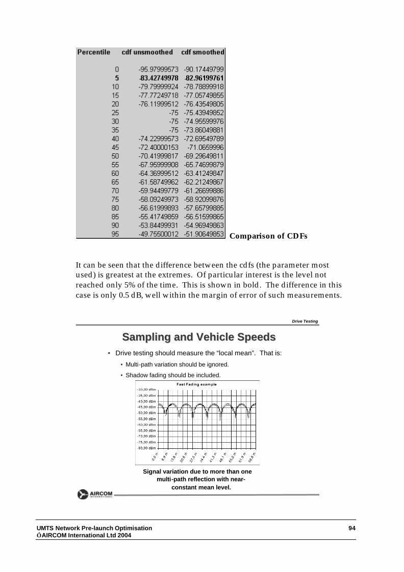
UMTS Network Pre-launch Optimisation 94 AIRCOM International Ltd 2004
Comparison of CDFs
It can be seen that the difference between the cdfs (the parameter most used) is greatest at the extremes. Of particular interest is the level not reached only 5% of the time. This is shown in bold. The difference in this case is only 0.5 dB, well within the margin of error of such measurements.
Sampling and Vehicle SpeedsSampling and Vehicle Speeds
Drive Testing
• Drive testing should measure the “local mean”. That is:
• Multi-path variation should be ignored.
• Shadow fading should be included.
Signal variation due to more than onemulti-path reflection with near-
constant mean level.

UMTS Network Pre-launch Optimisation 95 AIRCOM International Ltd 2004
Sampling and Vehicle Speeds: LeeSampling and Vehicle Speeds: LeeCriteriaCriteria
Drive Testing
• William Lee identified “ideal” measurement process:
• Average 36 samples over a distance of 40 λ to get a datapoint.
• Samples to be taken at least 0.8 λ apart
• This corresponds to:
• An averaging window of 5.6 metres.
• 36 samples taken at least 11 cm apart.
Using the ScannerUsing the Scanner
Drive Testing
• Scanners have a fixed sampling rate.
• However, it is “per reading”: if you are sampling 6channels the rate is one sixth.
• You either define an averaging period or post-process.
• E.g. Anritsu scanner:• Sampling period 10 ms per channel
• Typical number of channels: 6 (each channel now 60 ms)
• Averaging period can be set. 1 s typical.

UMTS Network Pre-launch Optimisation 96 AIRCOM International Ltd 2004
Using the ScannerUsing the Scanner
Drive Testing
• E.g. Anritsu scanner:• In order to get the averaging distance down to 5.6 metres, the
speed would have to be 20 kph.
Speed (kph) inter-sample distance (cm)
Samples per period
Averaging distance (m)
20 33 16.7 5 .640 67 16.7 11 .160 100 16.7 16 .780 133 16.7 22 .2
100 167 16.7 27 .8120 200 16.7 33 .3
Consequences of violating Lee CriteriaConsequences of violating Lee Criteria
Drive Testing
• Inter-sample distance too large:• Not in itself a problem (Lee specifies minimum distance), but
you have to fit in a large number of samples into the averagingdistance.
• Too few samples:• 36 samples predicted to give s.d. of 1 dB.
• 17 samples would give s.d of √(36/17) = 1.45 dB
• Note pilot power measurement accuracy quoted as ±2 dB.
• Averaging window too large:
• Miss sharp peaks and troughs
• Most appropriate value depends on environment.

UMTS Network Pre-launch Optimisation 97 AIRCOM International Ltd 2004
Consequences of violating Lee CriteriaConsequences of violating Lee Criteria
Drive Testing
• Varying the averaging window:
28 m averaging
-95
-90
-85
-80
-75
0 10 20 30 40
distance (m*28)
pilo
t st
reng
th d
Bm
pilot strength
5.6 m averaging
-95
-90
-85
-80
-750 50 100 150 200
distance (m*5.6)
leve
l in
dB
m
Pilot strength
28 metre averaging
5.6 metre averaging
Consequences of violating Lee CriteriaConsequences of violating Lee Criteria
Drive Testing
• Effect is to miss the extremes• Affects the cumulative distribution:
Cumulative distributions
-100
-95
-90
-85
-80
-75
-70
0 20 40 60 80 100
percentile
leve
l 5.6 m averaging
28 m averaging

UMTS Network Pre-launch Optimisation 98 AIRCOM International Ltd 2004
Lee Criteria: ConclusionsLee Criteria: Conclusions
Drive Testing
• Do not issue a global recommendation for 20 kph drivetest speeds. However:
• If the coverage in certain areas causes concern, and requires adetailed investigation, there are ways of maximising accuracyand confidence in measurements.
• There is no point in correcting a measured value of -68 dBmpilot (very good) to, say, -72 dBm (still very good).
Drive Test measurements: the need forDrive Test measurements: the need foraveragingaveraging
Drive Testing
• If you simply take “spot” measurements, you will includemultipath variations.
best server
-120
-100
-80
-60
-40
-20
00 5000 10000
best server
best svr moving average (20)
-100
-80
-60
-40
-20
00 5000 10000
best svrmovingaverage (20)
Unsmoothed data Smoothed data

UMTS Network Pre-launch Optimisation 99 AIRCOM International Ltd 2004
The need for averagingThe need for averaging
Drive Testing
• C.d.f. reveals differences.
Only 0.5 dB difference atcrucial 5% (95% betterthan) level.
Averaging can make filesizes more manageable(they can be enormous)and speed analysis as aresult.
6.8 Interpretation of Measurements
It is not sufficient to know what measurements can be made. The optimisation engineer needs to be able to interpret measurements to identify problems, choose the most appropriate measure to rectify the problem, and identify the best method for enhancing network performance. This will often entail taking a number of KPI’s in conjunction. For example, it is often necessary to know the condition of the uplink and of the downlink when choosing between alternative proposed methods of network optimisation.
For example, a drive test in undertaken during the busy hour in a live network. The test route is 100 metres in length along a route such that the distance to the nearest cell remains approximately constant. The following KPIs are extracted from the measured data.

UMTS Network Pre-launch Optimisation 100 AIRCOM International Ltd 2004
Ec/No Serving Cell -11 dB
Ec/No Neighbour 1 -20 dB
Ec/No Neighbour 2 -22 dB
Average Uplink Channel Power +21.4 dBm
Average Downlink Total Traffic Channel Power +39.6 dBm
Note the maximum uplink channel power is 23 dBm and the maximum total downlink channel power is 42 dBm.
What can an intelligent look at such results reveal? Firstly, the cell is under stress (which is probably why the drive test was performed). We can see from the pilot measurements that there is only one dominant serving cell. We are near the edge of the cell from the uplink coverage viewpoint (dangerously near judging by the uplink power levels recorded). Let us assume that the reason for carrying out the drive test was because coverage levels were reported as poor in this particular road. What methods would you recommend for improving this coverage?
We should consider the cost-benefit implications of any possible solutions:
Additional Site Very expensive – last resort
Mast Head Amplifier Cheapest Solution – probably
Uplink Diversity More expensive than MHA but capacity benefits
If we narrow down the possibility to either installing an MHA or implementing uplink diversity we need to establish the benefits that each would bring. When considering UL diversity, the possibility of increasing capacity must be assessed. In this circumstance a load will be transferred to the downlink. However, the data received shows that the downlink traffic power is near its limit and that the downlink would become the limiting factor if UL diversity was implemented. The MHA appears to be an attractive, rapid, relatively cheap solution – but – would it work? It is possible for the MHA to offer no improvement at all. Remember that a MHA only offers improvement if there is a noise problem to start with, probably caused by high feeder loss. If such circumstances exist, then an improvement of about 2 dB can be expected (an exact calculation is possible). This level of improvement should reveal itself through a

UMTS Network Pre-launch Optimisation 101 AIRCOM International Ltd 2004
subsequent drive test with the UE transmit power being lower than before the MHA was installed.
Alternative solutions: a still-cheaper solution would be to simply reduce the Noise Rise limit of the cell by 2 dB or so. It is significant that the test was done at the busy time of day when the cell Noise Rise level would be at or near its limit. Reducing the limit will have a coverage benefit but will reduce the capacity. It is important to realise that the amount by which it reduces the capacity depends on the original setting. If the original setting was 3 dB then reducing it by 2 dB would reduce the maximum loading factor from 50% to 21%. If however the original setting was 10 dB then the loading factor reduction would be from 90% to 84%, a much less severe reduction. If coverage is crucial to the area under test and is being judged as unsatisfactory, this might well be the short term solution to adopt whilst an MHA is ordered and installed.
Drive Test EquipmentDrive Test Equipment
• Some equipment suppliers• Anritsu
• http://www.eu.anritsu.com
Drive Test Measurement
•Portability and ease of setup prove to be thestrongest points of the Anritsu scanner.
•The Anritsu scanner was very simple to set up
•The information collected, although limited toRSCP, Ec/Io and SIR measurements for up to 32received scrambling codes.
•The receiver sensitivity was found to be betterthan that of the Agilent scanner- measuring RSCPsignal levels as low as -122dBm.

UMTS Network Pre-launch Optimisation 102 AIRCOM International Ltd 2004
Drive Test EquipmentDrive Test Equipment
• Some equipment suppliers• Agilent
• http://we.home.agilent.com/
Drive Test Measurement
•The extensive amount of output information
•Although more complicated in terms of setup
•Agilent scanner provides the user with moremeasured information and additional graphicalfunctionality.
•A strong solution but has limited sensitivity andis not hand portable.
Drive Test PlanningDrive Test Planning
• Pre-planning of drive test routes• Knowledge of network
•Site location
•Site configuration
• Knowledge of location
•Towns
•Terrain
• Operator known issues
•GSM problem areas
Drive Test Measurement

UMTS Network Pre-launch Optimisation 103 AIRCOM International Ltd 2004
Test-mobile MeasurementsTest-mobile Measurements
• A known CPICH transmit power inconjunction with the CPICH RSCP andUTRA carrier RSSI would allow thecalculation of pathloss to the cell andallow an estimation of cell dominance inidle mode.
• Estimate of the orthogonality of thedownlink is still problematic
• Drive test data is essential to validatepropagation models.
Drive Test Measurement
Drive Test MeasurementsDrive Test Measurements
• Prediction Assessment• Test Site Comparison
• Comparison of model against drive test measurements ofsite not used in the calibration process
• Drives vs. Predicted Best Server• Comparison between predicted and measured best
servers
• Drives vs. Predicted Pilot Pollution• Comparison between predicted and measured pilot
pollution
Drive Test Measurement

UMTS Network Pre-launch Optimisation 104 AIRCOM International Ltd 2004
• Test Site Comparison• Drive Test data compared with 3g calibration tool
• Analysis should provide both mean and standard deviation agreement
• For example– Mean error of 1.8dB– S.D of 7.9– Is a good practical fit
• Drives vs. Predicted Best Server• Exposes discrepancies with map data and local features
• Mud banks, rocks,
• Exposes limitations in antenna models and propagation model
• Drives vs. Predicted Pilot Pollution• Will highlight regions of multipath interference, difficult to calculate
Drive Test Measurement
Drive Test Measurements AnalysisDrive Test Measurements Analysis
Test-mobile MeasurementsTest-mobile Measurements• The commonly identified KPIs are not in themselves appropriate for
pre-launch optimisation and acceptance
• Test-mobile measurements, depending on the availability ofengineering mobiles, should allow measurement of:
• CPICH and P-CCPCH availability
• DCH - Dedicated channel DL performance• Cell dominance
• Active set size
• Required UL Tx Power
• These measurements would be possible under both loaded andunloaded conditions
Drive Test Measurement

UMTS Network Pre-launch Optimisation 105 AIRCOM International Ltd 2004
Interpretation of MeasurementsInterpretation of Measurements
• It is not sufficient to know what measurements can be made.
• The optimisation engineer needs to be able to interpret measurements
• This will often entail taking a number of KPI’s in conjunction.
• For example, lets imagine a drive test
• The test route is 100 metres in length along a route such that the distance to thenearest cell remains approximately constant.
• The following KPIs are extracted from the measured data.
Drive Test Measurement
+39.6 dBmAverage Downlink Total TrafficChannel Power
+21.4 dBmAverage Uplink Channel Power
-22 dBEc/No Neighbour 2
-20 dBEc/No Neighbour 1
-11 dBEc/No Serving Cell
• maximum uplink channel power is 23 dBm
• maximum total downlink channel power is 42 dBm.
Interpretation of MeasurementsInterpretation of Measurements
• The cell is under stress
• Uplink power is close to maximum
• There is only one dominant serving cell.
• Pilot levels of other cells are much lower than main cell
• We are near the edge of the cell from the uplink coverage viewpoint
• Uplink power is close to maximum
• Let us assume that the reason for carrying out the drive test was because
coverage levels were reported as poor on this particular road.
• What methods would you recommend for improving this coverage?
Drive Test Measurement

UMTS Network Pre-launch Optimisation 106 AIRCOM International Ltd 2004
Possible ActionsPossible Actions
• Mast head Amplifier
• Only reduces feeder loss and can introduce DL
problems due to insertion loss - may already be fitted
as standard.
• Transmit Diversity
• Will increase load on DL and with fast moving traffic
has little effect.
• Additional Site
• Very expensive option and should be last on list
• Reduce Noise Rise Limit
• Reduction of noise rise limit will increase coverage but
will reduce total capacity.
Drive Test Measurement

UMTS Network Pre-launch Optimisation 107 AIRCOM International Ltd 2004
7 The Pre-launch Optimisation Procedure
7.1 Introduction Following the planning and building of the network, it is essential that methodical steps are taken to ensure that the network performance is rapidly brought to a level deemed acceptable for launching. This involves:
• Hardware checks
• Configuration checks
• Coverage and Interference Optimisation
7.2 Hardware Checks It is essential that any hardware faults are eliminated. This is usually done on a cluster by cluster basis. Further, this can be said to be the responsibility of the equipment vendor. However, it is vital that the operator is confident in the procedure and in its ability to certify the equipment.
7.3 Configuration Checks Any attempt to optimise to a particular plan will be futile if the network has not been built to the plan. Care should be taken to ensure that the network is built “as intended”. This includes verifying the:

UMTS Network Pre-launch Optimisation 108 AIRCOM International Ltd 2004
The site is in the correct location
Antenna is of the correct type
Antenna height, azimuth and tilt are all as planned
The feeder is of the correct type and length
Cell parameters (common channel powers etc.) are in accordance with the plan.
7.4 Optimisation Team Structure In order to ensure that the optimisation runs smoothly and efficiently, it is essential that the staffing levels are appropriate to sustain the workflow. A typical RNC area serving 100 sites would require the following analysis team:
Systems Analysis Engineers: x3
Driver Test Radio Engineers: x2
Drivers: x2
Configuration Engineer: x1
Pre-launch OptimisationPre-launch Optimisation
• Following planning and building of network:• Perform Hardware Check• Check cell configuration for conformity with plan
• Bring coverage and interference levels up toagreed thresholds
Pre-launch Optimisation

UMTS Network Pre-launch Optimisation 109 AIRCOM International Ltd 2004
Pre-launch OptimisationPre-launch Optimisation
• Perform Hardware Check:• It is essential that any hardware faultsare eliminated.
• This is usually done on a cluster bycluster basis.
• Can be said to be the responsibility of theequipment vendor.
• However, it is vital that the operator isconfident in the procedure and in itsability to certify the equipment.
Pre-launch Optimisation
Pre-launch OptimisationPre-launch Optimisation
• Perform Cell Configuration Check:• The site is in the correct location• Antenna is of the correct type• Antenna height, azimuth and tilt are all as
planned• The feeder is of the correct type and length• Cell parameters (common channel powers etc.)
are in accordance with the plan.
Pre-launch Optimisation

UMTS Network Pre-launch Optimisation 110 AIRCOM International Ltd 2004
Optimisation Team StructureOptimisation Team Structure
• Each RNC area has:• Drive Test Team
• Systems Analysis Team (SAT)
• Configuration Engineer
Pre-launch Optimisation
The Structure - Drive Test TeamThe Structure - Drive Test Team
• Drive representative routes gathering:• Scanner data (rooftop mounted calibrated antenna)
• Mobile (UE) data (test mobile on rear seat connected tolaptop)
• Scanner provides accurate measurements of pilot strengthetc.
• UE data provides evidence of call success and uplink Txpower.
• Drive test data is passed to the SAT team.
Pre-launch Optimisation

UMTS Network Pre-launch Optimisation 111 AIRCOM International Ltd 2004
The Structure - The SAT teamThe Structure - The SAT team
• In addition to defining the drive test routes:
• The SAT team process the data to provide• summative results (CCSR, c.d.f of pilot strength
etc.)
• diagnoses of problems.
• Problems are resolved through close liaisonwith the configuration engineer.
Pre-launch Optimisation
The Structure - The configuration engineerThe Structure - The configuration engineer
• The Configuration engineer• monitors the state of the network
• requests changes to network configuration(antenna orientation etc.)
• tracks changes through the system
Pre-launch Optimisation

UMTS Network Pre-launch Optimisation 112 AIRCOM International Ltd 2004
The Structure The Structure -- exampleexample
• Drive test reveals calls dropped in an area where best pilot is very low.
• SAT team checks with configuration engineer regarding cell status
• Check made with planning tool to see whether problem is “predictable”
• If no obvious reason, SAT directs drive test team to investigate.
Pre-launch Optimisation
The Structure The Structure -- example (continued)example (continued)
• Drive test team report that an obstacle/terrain feature exists that is not on map data.
• SAT team recommend solution (antenna height/orientation)
• Effect checked on planning tool
• Configuration Engineer actions change and reports when implemented.
• SAT instructs drive test team to re-examine
Pre-launch Optimisation
7.5 Using Drive Test Data

UMTS Network Pre-launch Optimisation 113 AIRCOM International Ltd 2004
Drive Testing has been described in the previous chapter. Typical goals (“key parameters”) for a suburban area are:
• 95% of the area should be measured so that the pilot is better than –99 dBm (-89 dBm for a dense urban area).
• 95% of the coverage area should have a measured Ec/Io of better than –10 dB (quiet network)
In reaching these goals, the Systems Analysis engineer will need to adopt other, intermediate, parameters to assist in identifying the cause of any problems. Coverage and interference can, to a certain extent, be treated separately but effects on interference must be considered when addressing coverage problems and vice versa.
7.5.1 Coverage problems
Suppose that the coverage measurements do not meet the necessary criterion. The procedure can be summarised as follows:
• Identify coverage holes
• Assess the most serious of those and rank in order of priority
• Rectify problems in priority order until criterion is met.
The issue as to which coverage hole is most serious is usually a matter of identifying the percentage of the total “low signal strength area” that can be attributed to one particular hole. It is important that this percentage is on the basis of area or route length rather than number of readings. If the number of data points is taken then the statistics are distorted in favour of the regions where the drive-test vehicle was travelling slowly (or stopped). A map view is vital in assessing this. Once the areas to be rectified have been identified the question “does the planning tool predict that this hole will exist?” should be asked:
If the answer to this is “yes” then the thinking behind this must be questioned. Pre-launch optimisation cannot achieve the impossible. It can only optimise to a planned performance. The outcome of discussion should be either a decision to either remove the area in question from the coverage requirements, or to re-visit the plan.
If the answer is that the hole was unexpected then further investigation is required. The first thing to ascertain is which cell would be expected to provide coverage in the area. A check should be made to ensure that this cell was active at the time of the drive-test measurement. This can be done either by examining the drive test data to see that the cell in question was transmitting (i.e. the pilot was “low” rather than non-existent) or, if necessary, confirming with the configuration team that the site and cell were active. It is possible that a fault has occurred in

UMTS Network Pre-launch Optimisation 114 AIRCOM International Ltd 2004
the feeder and antenna arrangement causing an increase in path loss. Using a feeder and antenna calibration tool such as Anritsu Site Master can check this. The hole in coverage could well be due to a local anomaly in the site configuration or environment. A first step is to identify which cell should be providing coverage at the location. A combination of use of the planning tool and measurement of the strongest pilot can identify this (the less you have to change the better). Perhaps there is an obstacle that is not considered by the propagation model. It is possible that the configuration of the site itself causes the problem. If antennas are set back from the edge of a large roof, for example, the building can cause shadows near to the base of the site. Assessment of the problem should result in a plan of action that could include:
• Change site configuration
Antenna height (almost certainly restricted)
Antenna location
Antenna azimuth/downtilt (the most common change made in the initial stages)
Substitute antenna for one of higher gain
• Introduce new site
A “last resort” (expensive) but not unheard of.
7.5.2 Interference issues
Once coverage has been addressed, the area covered should be investigated to ascertain that interference is at acceptable levels. The expectation is that the network will be very lightly loaded when the testing is undertaken and, in those circumstances, it is expected that Ec/No should be better than approximately –10 dB. If we consider a location where the pilot is –95 dBm, “No” could be as high as –85 dBm. If the level of thermal noise is around the –102 dBm level, then the only way that Ec/No can fail to meet the required level is if the levels of interference from within the network are too high. Poor Ec/Io is almost always a result of “over propagation”. That is, cells that are not required to provide coverage in a particular area are delivering high signal strength (that, because it is not necessary for coverage, can be regarded as co-channel interference). The procedure to rectify this can be described as follows:
Identify the worst affected areas: note that, if Ec/No is worse than about –14 dB it could result in call drops even with the network lightly loaded. The level of –10 dB with the network lightly loaded indicates that problems could occur if the network became heavily loaded.

UMTS Network Pre-launch Optimisation 115 AIRCOM International Ltd 2004
Investigate to identify the strength of measurable pilots in that area. An Ec/Io of worse than –10 dB indicates that there are more than three significant pilots. Given the structure of a cellular network, it is inevitable that there will be areas where three near equal pilots exist. If the network is lightly loaded, this would cause Ec/No to drop to about – 7 dB. Any additional pilots can be considered as “polluters” that should be reduced in strength at the location in question. In order to identify potential problem areas, it is probably good practice to investigate areas that have Ec/Io worse than, say, -8 dB when the network is quiet. A further check is to highlight and investigate areas where there are more than two other pilots within, say, 8 dB of the best server. Even if these areas do not threaten a call drop, the out of cell interference will reduce the network capacity.
Coverage and Interference GoalsCoverage and Interference Goals
• Typical Criteria:• 95% of area delivers pilot strength of >-89dBm (dense urban) or -94 dBm (urban).
• 95% of area covered should register Ec/Nobetter than -10 dB.
Pre-launch Optimisation

UMTS Network Pre-launch Optimisation 116 AIRCOM International Ltd 2004
Improving Coverage: ProcedureImproving Coverage: Procedure
• From drive-test data:• Identify coverage holes• Assess the most serious of those and rankin order of priority
• Rectify problems in priority order untilcriterion is met.
Pre-launch Optimisation
Improving InterferenceImproving Interference
• Within covered area (i.e. pilot better thanrequired threshold) attaining a Ec/No betterthan -10 dB is “easy” (perhaps -9 or -8 wouldbe a better target) if the network is lightlyloaded.
• If pilot strength is -95 dBm, noise plusinterference must be -85 dBm (thermal noise)
• Even in an area where there are three equalpilots and common channel power equals pilotpower, pilot Ec/No should be 1/6 or -8 dB.
Pre-launch Optimisation

UMTS Network Pre-launch Optimisation 117 AIRCOM International Ltd 2004
Improving InterferenceImproving Interference
• Scanner Data.
• Area wherethere are threeequal low-levelpilots revealsEc/Io of -8 dB.
Pre-launch Optimisation
Improving InterferenceImproving Interference
• Scanner Data.
• Area where thereare seven low-level pilots (notequal strength).
• Best Ec/Io =-10 dB
Pre-launch Optimisation

UMTS Network Pre-launch Optimisation 118 AIRCOM International Ltd 2004
Improving InterferenceImproving Interference
• Typical drive test result from well-optimisedcluster.
Pre-launch Optimisation
Ec/Io >-12 dB 99.91%Ec/Io >-11 dB 99.44%Ec/Io >-10 dB 98.14%Ec/Io >-9 dB 94.97%Ec/Io >-8 dB 89.44%Ec/Io >-7 dB 81.22%Ec/Io >-6 dB 68.83%Ec/Io >-5 dB 53.66%Ec/Io >-4 dB 34.94%Ec/Io >-3 dB 13.46%
• -9 dB seems to be more appropriate threshold.
Improving Interference: ProcedureImproving Interference: Procedure
• Identify areas of low Ec/Io• Examine pilot levels (there will probably
be more than three).• Identify any unwanted pilots (from cells
that are not intended to provide coveragein that area).
• Reduce level of these pilots (usually bydown-tilting)
•be aware of the effect on coverage inservice area of cell: use planning tool.
Pre-launch Optimisation
7.6 The need for consistency Drive test measurements are at the heart of the optimisation process. It is vital that they can be relied upon. Measuring the pilot level is considerably more complicated than measuring a carrier wave (CW)

UMTS Network Pre-launch Optimisation 119 AIRCOM International Ltd 2004
signal. As a result it is not spectacularly accurate, ± 2 dB being quoted by manufacturers. The process physical optimisation of the network can be simplified and summarised as:
• Measure the performance
• Change cell configurations
• Measure again to confirm improvement
The need for consistency between procedures for the two measurement activities is clear. Possible inconsistencies are:
• Different (uncalibrated) antenna/feeder
• Different drive test route
• Different UE speed over drive test route (hold ups at traffic lights etc.)
• Different measurement equipment.
Striving to maintain a consistent approach will result in the most reliable measured data.
Drive Test Data: the need for consistencyDrive Test Data: the need for consistency
• Optimisation of physical aspects, in summary:• Measure the performance
• Implement configuration changes
• Measure again to show improvement.
• Clearly there is a need for consistency
Pre-launch Optimisation

UMTS Network Pre-launch Optimisation 120 AIRCOM International Ltd 2004
Drive Test Data: the need for consistencyDrive Test Data: the need for consistency
• Potential for inconsistency:• Different (uncalibrated) antenna/feeder
• Different drive test route
• Different UE speed over the route (hold ups attraffic lights etc.)
• Different analyser being used.
• Different level of network loading (affects Ec/Io).
Pre-launch Optimisation
Drive Test Data: the need for consistencyDrive Test Data: the need for consistency
• Ideally:• Use the same analyser, feeder and antenna for the
“before” and “after” measurements.• Ensure that you keep to the same route.
• Be consistent regarding UE speed. Sample dataon a distance, rather than time, basis. If this is notrealistic, try and pause sampling when held up inheavy traffic.
• Check to see if load testing is going on in this area.Make measurements at the same time of day to getnear-equal loading conditions.
Pre-launch Optimisation
7.7 Using drive test data to tune Neighbour list

UMTS Network Pre-launch Optimisation 121 AIRCOM International Ltd 2004
Identifying Suitable Neighbours - usingIdentifying Suitable Neighbours - usingdrive testsdrive tests
NCELLS
• It is clear that drive test results will be a valuableresource when planning neighbour (Ncell) lists.
• These should give details regarding the experiencewithin the coverage area of a cell.
• Potential Ncells can then be assessed.
• Fine resolution required - just a “drive through” of acell is not sufficient.
Identifying Suitable Neighbours - usingIdentifying Suitable Neighbours - usingdrive tests: an exampledrive tests: an example
NCELLS
• A cell was identified as suitable for testing theusefulness of drive tests.

UMTS Network Pre-launch Optimisation 122 AIRCOM International Ltd 2004
Identifying Suitable NeighboursIdentifying Suitable Neighbours
NCELLS
• Scrambling codes of these Ncells were noted.
• Serving cell has SC 8.
Cell Scrambling Code Overlap1895011 0 Co-site1895031 16 Co-site2215031 88 17%0089011 24 1.5%1164011 48 1.3%6985031 112 0.5%
• Planning tool was used to plan neighbours.
• 2 co-sited cells plus four “interfering” cells are registered.
Identifying Suitable NeighboursIdentifying Suitable Neighbours
NCELLS
• Scrambling codes of these Ncells were noted.
• Serving cell has SC 8.
Cell Scrambling Code Overlap1895011 0 Co-site1895031 16 Co-site2215031 88 17%0089011 24 1.5%1164011 48 1.3%6985031 112 0.5%

UMTS Network Pre-launch Optimisation 123 AIRCOM International Ltd 2004
Identifying Suitable NeighboursIdentifying Suitable Neighbours
NCELLS
• Drive Test undertaken: scanner results recorded onTEMS and Anritsu.
Question 1.How often did was each pilot received at a level within 10 dB of SC 8?
Number of hits (Anritsu scanner):Scrambling Code Number of hits0 26448 8024 46112 4216 3788 9
Identifying Suitable NeighboursIdentifying Suitable Neighbours
NCELLS
Question 2How often was each pilot the second best server?
Number of hits (TEMS scanner)Scrambling Code Number of hits0 382348 10724 99112 2816 61288 7

UMTS Network Pre-launch Optimisation 124 AIRCOM International Ltd 2004
Identifying Suitable NeighboursIdentifying Suitable Neighbours
NCELLS
Question 3How often was each pilot third best server?
Number of hits (TEMS scanner)Scrambling Code Number of hits0 408348 35024 142112 8316 588 7
Identifying Suitable NeighboursIdentifying Suitable Neighbours
NCELLS
Question 4How often did each pilot replace SC 8 as the strongest pilot, and vice versa?
Number of hits (TEMS scanner)Scrambling Code Number of hits0 114648 15924 128112 3716 14588 2

UMTS Network Pre-launch Optimisation 125 AIRCOM International Ltd 2004
Identifying Suitable NeighboursIdentifying Suitable Neighbours
NCELLS
Notes on processing the data
The TEMS data was much faster to process than the ANRITSU. This was due mainly to tworeasons:
1. TEMS outputs SCs as a simple number rather than a code2. TEMS always lists the pilot strengths in descending order of measured power level. Anritsu is
more random.
The TEMS logfile was exported using the tex template TEMS_2.1_ExportFile_UE.tex
Identifying Suitable NeighboursIdentifying Suitable Neighbours
NCELLS
• Conclusions.
• A simple treatment of TEMS scanner data resulted in what appears to be agood neighbour list. It is also a short list. Further, the prioritisation order ofthe neighbours if necessary is clear.
• Note that approximately 1 hour of driving is required fora single cell.
7.8 Load Testing of a Network The network will be required to service a certain level of demand. The cell configuration selected will impose a limit on the capacity of that cell. This is known as a hard blocking limit. It can be thought of as a limit in the total user throughput that the cell can accommodate. An extra limitation is imposed by interference within the air interface (soft blocking). If the network is quiet, the air interface capacity

UMTS Network Pre-launch Optimisation 126 AIRCOM International Ltd 2004
should be high and a load test on a single cell should allow the hard blocking limit to be reached. Testing to confirm this involves ensuring many UEs are simultaneously active on the cell. As voice (employing discontinuous transmission) and packet services transmit intermittently, video telephony (VT) calls are usually used to assess the ability of the network to accommodate a high throughput. A typical VT call is active 100% of the time and transmits at 64 kbit/s. Thus if a cell was capable of sustaining 800 kbit/s should allow 12 VT calls to be simultaneously active on a single cell. In order to conduct a straightforward assessment of the cell capacity, the tests can be done with the UEs stationary. (A “routiner” is a piece of equipment that controls UEs and performs prescribed tasks from a fixed location). However, some mobility of the UEs can be tested for in order to assess the impact. Similarly, tests should be conducted in different Ec/Io environments. Low Ec/Io may result in air interface imposing “soft” blocking on the network. Mobility tests the power control system which again has implications for the loading on the air interface. Any discrepancy between the predicted and achieved cell capacity should be investigated. Such an investigation will include examining the reasons for failure. These reasons could include air interface problems such as interference levels higher than expected and/or hardware issues.
Drive Tests: load testing a cellDrive Tests: load testing a cell
Pre-launch Optimisation
• The cell capacity can usually bedefined as a total possible user datarate (hard blocking)
• Air interface capacity is interferencelimited (soft blocking)
• In a lightly loaded network, it shouldbe possible to achieve the hardblocking limit.
• Video telephony (VT) is probablybest way of testing as it is:
• always on (100% activity factor)
• High unit resource (64 kbps)
•Drive test
•Load test

UMTS Network Pre-launch Optimisation 127 AIRCOM International Ltd 2004
Drive Tests: load testing a cellDrive Tests: load testing a cell• E.g. if hard limit is user data rate of
800 kbps, 12 simultaneous VT callsshould be possible.
• Varying degrees of mobility can beassessed.
• A “routiner” controls UEs andperforms prescribed tasks from astatic location.
• Discrepancies between predictionsand results must be analysed.
• Possible reasons for discrepanciesinclude interference and hardwareissues.
•Drive test
•Load test
Pre-launch Optimisation
Drive Tests: load testing a cellDrive Tests: load testing a cell• Tests can be done in different
“environments: most importantly atdifferent levels of Ec/Io within thecoverage area.
• Areas of low Ec/Io may lead to theair interface capacity beingreduced with resulting “softblocking”.
• Mobility will affect the power controlsystem, again with implications forthe soft capacity of a cell.
•Drive test
•Load test
Pre-launch Optimisation
7.9 Testing of a network for IRAT success When testing a UMTS network, it is common for mobiles to be locked onto UMTS. Thus Inter Radio Access Technology (IRAT) hand over is not tested. Successful IRAT is seen as crucial for a successful UMTS launch.

UMTS Network Pre-launch Optimisation 128 AIRCOM International Ltd 2004
It is therefore vital that tests are conducted in order to assess IRAT operation. It is proposed that tests be conducted in three distinct areas: • At coverage edge • In an urban environment • Traffic Hotspots Tests need to be conducted both in active and idle modes. In the initial phase of testing, it is proposed that active mode tests are voice calls only. Of particular importance is the occurrence of a call drop due to IRAT failure. Thus, calls will be continuous and monitored for either successful hand over or call drop. The procedure will need to be modified depending on the environment and each environment category will now be addressed in turn.
7.9.1 IRAT at coverage edge As a mobile moves to the edge of a UMTS coverage area it will need to perform a hand over to the GSM network. The initial stage is for the mobile to enter “compressed mode” at which point it can measure signal strengths on the GSM network. Then, if the measured Ec/No drops further, a hand over to GSM will be instigated. Thus, the drive test should involve driving from an area of good UMTS coverage to a point beyond the coverage area. The RF engineer should make a call at the beginning of the test and attempt to maintain this call. Call progress should be monitored for a successful GSM hand over (or call drop). Additionally, it is of value to know that the hand over was to an appropriate GSM cell. The existence of rapid hand overs within the GSM network immediately following IRAT hand over indicates that the initial GSM cell was not the most appropriate. Further, the GSM network should hold the call for an acceptable time. It is therefore proposed that the following data is logged:
7.9.2 Success of hand over Hand overs within the GSM network for the next 10 seconds should be monitored and the success of call holding within GSM network for the next 30 seconds should be checked. A successful IRAT hand over would be declared only if the call survives on the GSM network for a period of greater than 30 seconds after leaving the UMTS network.

UMTS Network Pre-launch Optimisation 129 AIRCOM International Ltd 2004
7.9.3 Designing the test route The test routes should be designed so that they involve the mobile leaving the UMTS coverage area. Such routes will be uni-directional when the voice call is active and bi-directional in active mode. As an indicator of the edge of coverage, areas where the predicted pilot strength is below –100 dBm should be used as an indicator. Initially only Motorways, Class “A” and Class “B” roads should be used for routes.
7.9.4 IRAT in an urban environment. IRAT will also occur in areas where the UMTS network is interference limited. This could be due to excessive interference or the existence of coverage “holes” (especially indoors). Defining an appropriate neighbour list is again important. However, it is likely to be a somewhat frustrating area to test as it is not inevitable that an IRAT hand over attempt will be made. A UE can be “encouraged” to make an attempt by deliberately increasing the path loss by, perhaps, placing the mobile on the floor of the vehicle. An increase of about 6dB to 10dB would be appropriate. Experience will allow this to be assessed. A successful IRAT hand over will be judged on the same criteria as for the coverage edge areas. This test will require a high degree of alertness on the part of the RF engineer, as he will need to assess whether a hand over has occurred or the call has been dropped. Once either of these has happened it will be necessary to start a new call having camped in idle mode to UMTS. . Again, the test will need to involve both active and idle UEs. In the case of idle UEs however, the testing can be automated as IRAT reselection should occur in both directions.
7.9.5 Designing the test route. It is envisaged that test routes already devised for assessing coverage for a site “cluster” (see section 6) will be appropriate for IRAT testing.
7.9.6 IRAT at hotspots. The experience in traffic hotspot areas is of high significance as such areas generate disproportionately large revenue. The set up procedure is similar to that for the urban area. However, testing will be undertaken at a slower mobile speed. Again, the path loss to the mobile may well need to be increased artificially by roughly 6dB to 10dB in order to encourage IRAT hand over to occur. Testing should be undertaken both in active and idle mode with a procedure similar to that used for the urban area being adopted.
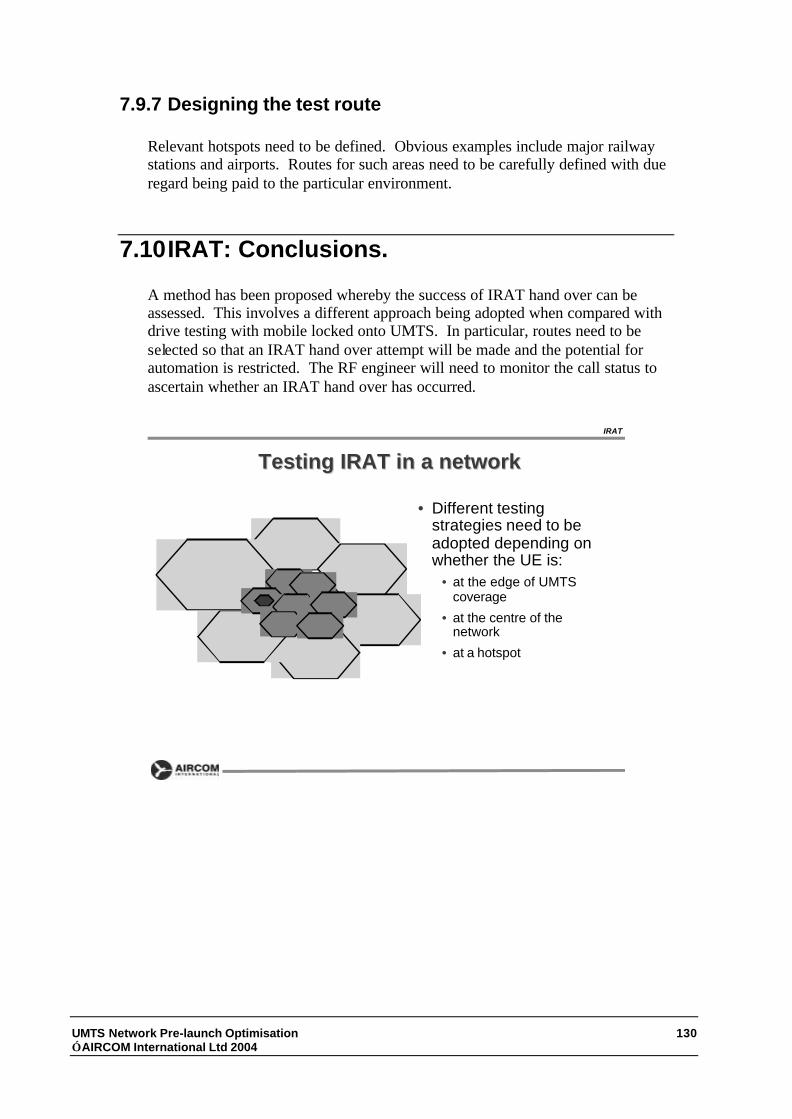
UMTS Network Pre-launch Optimisation 130 AIRCOM International Ltd 2004
7.9.7 Designing the test route Relevant hotspots need to be defined. Obvious examples include major railway stations and airports. Routes for such areas need to be carefully defined with due regard being paid to the particular environment.
7.10 IRAT: Conclusions. A method has been proposed whereby the success of IRAT hand over can be assessed. This involves a different approach being adopted when compared with drive testing with mobile locked onto UMTS. In particular, routes need to be selected so that an IRAT hand over attempt will be made and the potential for automation is restricted. The RF engineer will need to monitor the call status to ascertain whether an IRAT hand over has occurred.
Testing IRAT in a networkTesting IRAT in a network
IRAT
• Different testingstrategies need to beadopted depending onwhether the UE is:
• at the edge of UMTScoverage
• at the centre of thenetwork
• at a hotspot

UMTS Network Pre-launch Optimisation 131 AIRCOM International Ltd 2004
Testing at a cell edgeTesting at a cell edge
IRAT
• In active mode: drive will beuni-directional
• In idle mode: drive should bebi-directional
• Active mode: make acontinuous call
• monitor for IRAT hand over (orcall drop)
• monitor rapid GSM hand oversafter IRAT (10 seconds)
• check GSM network sustainsconnection (30 seconds)
• Route should initially berestricted to Motorways, ‘A’roads and ‘B’ roads.
Testing at a network centreTesting at a network centre
IRAT
• IRAT can be required due tocoverage holes (especiallyindoors) or excessiveinterference.
• Not inevitable that IRAT willoccur.
• Mobile can be “encouraged”to enter IRAT mode (placedon floor of vehicle?)

UMTS Network Pre-launch Optimisation 132 AIRCOM International Ltd 2004
Testing at a network centreTesting at a network centre
IRAT
• RF engineer must monitorevents closely
• Calls will be continuous butmust be re-started manuallywhen IRAT has occurred.
• Test route similar to thatadopted for “bubbleoptimisation” process isprobably suitable.
Inter Radio Access Technology (IRAT)Inter Radio Access Technology (IRAT)Consideration of Ec/No valuesConsideration of Ec/No values
IRAT
• A UE should perform a hand over to GSM when Ec/Nodrops below a particular value.
• Any records of Ec/No below this threshold may indicatea problem.
Number of Records
Ec/No
Threshold
-6 -7 -8 -9 -10 -11 -12 -13

UMTS Network Pre-launch Optimisation 133 AIRCOM International Ltd 2004
ConclusionsConclusions
IRAT
• Urgent requirement exists forthe IRAT success rate to beassessed.
• Drive tests must beundertaken accordingly.
• Initial selection of routesinfluenced bycharacterisation feedback.
Inter-technology Neighbour Lists:Inter-technology Neighbour Lists:PlanningPlanning
IRAT PLANNING
• Likely strategy:• Make co-sited GSM cell a neighbour
• Make neighbours of this cell a neighbour
• Manually adjust “as appropriate”.
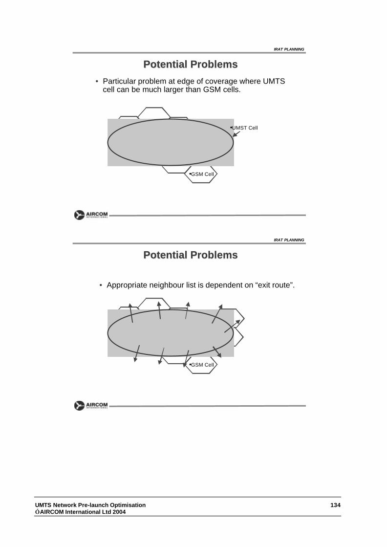
UMTS Network Pre-launch Optimisation 134 AIRCOM International Ltd 2004
Potential ProblemsPotential Problems
IRAT PLANNING
•UMST Cell
•GSM Cell
• Particular problem at edge of coverage where UMTScell can be much larger than GSM cells.
Potential ProblemsPotential Problems
IRAT PLANNING
•GSM Cell
• Appropriate neighbour list is dependent on “exit route”.

UMTS Network Pre-launch Optimisation 135 AIRCOM International Ltd 2004
A SuggestionA Suggestion
IRAT PLANNING
•GSM Cell
• Cells at the edge of coverage are severely down-tiltedand/or pilot power adjusted to control coverage area
A SuggestionA Suggestion
IRAT PLANNING
•GSM Cell
• This would have further advantage of offering “immunityto cell breathing”.
• Testing and optimising of this should be made a priority.


UMTS Network Pre-launch Optimisation 137 AIRCOM International Ltd 2004
8 Functional Testing
8.1 Introduction
If coverage and interference levels meet the targets and the neighbour list for each cell is correctly set, then it could be said that there is “no excuse” for calls to drop (or fail to set up) within a network when a drive-test making live calls is made, particularly if the network is lightly loaded and the UE is in a car rather than within a building. However, getting 100% success with voice, video telephone and packet services is highly unlikely. Failures should be analysed to identify the cause. The causes can be divided into different categories:
• Coverage or interference problem
• Hand over failure
• Network problem
• Handset issue
8.1.1 Coverage/Interference Problem
The measurements we make attempt to ensure a low probability of the path loss or interference levels becoming too high to sustain a call. However, it is not impossible that such a situation will occur. If such problems occur, the plan and drive test criteria for the areas in question require re-investigation. Further, it should be noted that all measurements have been performed on the downlink. The targets have been derived making suitable assumptions regarding the link budget in both directions. If there are problems with the receiver (such as the mast head amplifier being out of specification) it would invalidate these assumptions. Such problems can be indicated by monitoring the uplink

UMTS Network Pre-launch Optimisation 138 AIRCOM International Ltd 2004
UE transmit power. This will vary over a possible range of, typically, –49 dBm to +21 dBm. Any areas where records show that it is near its upper limit (e.g. >+11 dBm) should be investigated in connection with call drop problems.
8.1.2 Hand over failure
The neighbour list may be optimised yet hand over can still fail. The successful update of the active set requires a sophisticated sequence of operations to take place. Further, it is a time-dynamic process. The conditions on the air interface must be acceptable for a given amount of time to enable the hand over to take place. In particular, in situations where there is only one cell in the active set, the signal from this cell must remain sufficiently strong during a hand over event until a second cell can join the active set. A sudden decrease in the strength of the primary server can cause a call to drop. This can be influenced by the speed and direction of the UE as it travels through the hand over region. The area of the hand over region is a compromise: it has to be large enough to allow hand over to occur at reasonable speeds but, if it is too large, it can result in high interference within the network. That would reduce the network capacity. Clearly, measuring the exact area of the hand over regions throughout the network would be extremely time consuming. The recommendation is that problem areas are investigated when they come to notice. Rather than making a physical change, it is possible to adjust the hand over window such that a new potential server attempts to join the active set earlier.
8.1.3 Network problems
Occasionally, a call will drop or fail to establish for no apparent reason. It may be that the network suddenly issues an instruction to clear the call. These should be recorded and followed up with the network configuration team.
8.1.4 Handset issues
UMTS technology is still somewhat in its infancy. It may be that a call drop problem is specific to a particular UE. That is different UEs produce noticeably different drive test results. The rapid identification of such situations is crucial to ensure that time is not wasted investigating the cause of these problems.

UMTS Network Pre-launch Optimisation 139 AIRCOM International Ltd 2004
8.2 UE and UTRAN Measurements
The UE is capable of making and reporting measurements regarding power levels on the air interface in addition to control messages. These help us to identify the cause of any network failure.
UE MeasurementsUE Measurements• The UTRAN may control a measurement in the UE either
• By broadcast of SYSTEM INFORMATION
• And/or by transmitting a MEASUREMENT CONTROL message.
• The following information is used to control the UE measurements• Measurement identity: A reference number that should be used by
the UTRAN when setting up, modifying or releasing the measurementand by the UE in the measurement report.
• Measurement command: 1 of 3 different measurement commands.
• Setup: Setup a new measurement.
• Modify: Modify a previously defined measurement, e.g. tochange the reporting criteria.
• Release: Stop a measurement and clear all information in theUE that are related to that measurement.
• Measurement type
UE Measurements
Measurement TypeMeasurement Type• Intra-frequency measurements
• downlink physical channels at the same frequency as the active set.
• Inter-frequency measurements
• downlink physical channels at frequencies that differ from the frequency of the activeset and on downlink physical channels in the active set.
• Inter-RAT measurements
• downlink physical channels belonging to another radio access technology e.g. GSM.
• Traffic volume measurements
• uplink traffic volume.
• Quality measurements
• downlink quality parameters, e.g. downlink transport block error rate.
• A measurement object corresponds to one transport channel in the case of BLER.
• UE-internal measurements
• UE transmission power and UE received signal level.
• UE positioning measurements
• A measurement object corresponds to one cell.
UE Measurements

UMTS Network Pre-launch Optimisation 140 AIRCOM International Ltd 2004
The UTRAN itself makes measurements regarding the situation on the air interface. Many of these, such as the uplink load fall into the category of “key performance indicators” (KPIs).
UTRAN MeasurementsUTRAN Measurements• Received total wide band power
• If receive diversity is being used then take the average of the power
• Measurement period 100ms
• Range is -112dBm to -50dBm
• Signal to Interference Ratio SIR
• Measured on a DPCCH – Dedicated Physical Control Channel
• (RSCP / ISCP) x SF
• RSCP - Received Signal Code Power (of one code)
• ISCP - Interference Signal Code Power
• SF – Spreading Factor 256
• Measurement period 80ms
• Range -11 to 20 dB
Source TS 25.133
UTRAN Measurements
UTRAN Measurements – UTRAN Measurements – KPI’sKPI’s• KPI’s are calculated from active
measurements
• 3GPP standards define the UEand UTRAN measurements taken
• KPI’s will gather thesemeasurements and calculate anaverage value
• Average Uplink Load
∑∑=
RSSIP
LoadUplinkAverage tx
UTRAN Measurements
RSSI Receiving Signal Strength Indicator
o
T
TN
T
TN
N
o
N
IP
PPP
load
PPP
IP
load
NRload
=+
=
+−=−=
−=
11
11
Note: RBS cannot distinguish between in cell and out ofcell power when reporting RSSI

UMTS Network Pre-launch Optimisation 141 AIRCOM International Ltd 2004
UTRAN MeasurementsUTRAN Measurements• Signal to Interference Ratio SIR
• Measured on a DPCCH – Dedicated Physical ControlChannel
• (RSCP / ISCP) x SF
• RSCP - Received Signal Code Power (of one code)
• ISCP - Interference Signal Code Power
• SF – Spreading Factor 256
• Measurement period 80ms
• Range -11 to 20 dB Measuredquantity value
Reported value
20.0 = SIR dBUTRAN_SIR_6319.5 = SIR < 20.0 dBUTRAN_SIR_6219.0 =SIR < 19.5 dBUTRAN_SIR_61
…….-10.5=SIR < -10.0 dBUTRAN_SIR_02
-11.0 = SIR < -10.5 dBUTRAN_SIR_01SIR < -11.0 dBUTRAN_SIR_00
UTRAN Measurements
UTRAN MeasurementsUTRAN Measurements
• SIRerror = SIR – SIRtarget
• Measurement period 80ms
• Accuracy ±3dB
• Range -31 to 31 dB
31.0 = SIRerror dBUTRAN_SIR_ERROR_12530.5 = SIRerror < 31.0 dBUTRAN_SIR_ERROR_12430.0 = SIRerror < 30.5 dBUTRAN_SIR_ERROR_123
… … …0.0 = SIRerror < 0.5 dBUTRAN_SIR_ERROR_063-0.5 = SIRerror < 0.0 dBUTRAN_SIR_ERROR_062
… … …-30.5 = SIRerror < -30.0 dBUTRAN_SIR_ERROR_002-31.0 = SIRerror < -30.5 dBUTRAN_SIR_ERROR_001SIRerror < -31.0 dBUTRAN_SIR_ERROR_000
Measured quantity valueReported value
UTRAN Measurements

UMTS Network Pre-launch Optimisation 142 AIRCOM International Ltd 2004
UTRAN MeasurementsUTRAN Measurements• Transmitted carrier power
• Ratio of total transmitted power on one DL carrier to the maximum possible
power of this DL carrier, range 0 to 100%
• Measurement period 100ms
• Transmitted code power
• Measurement of the DPCCH field of any dedicated radio link
• Measurement period 100ms
• Range -10 to 46 dBm
• Reflects the power on the pilot bits of the DPCCH field
• Transmitted channel BER – range 0 to 1
• Physical channel BER – range 0 to 1
UTRAN Measurements
UTRAN MeasurementsUTRAN Measurements• SFN-SFN observed time difference – Synchronisation
• Measurement period 100 ms
• Range -19200 to 19200 chip
• Round trip time
• RTT = Trx – Ttx
• Trx – time of reception of DPCCH/DPDCH from UE
• Ttx – time of transmission of DL DPCH to a UE
• Measurement period 100ms
• Range 876.0000 to 2923.8750 chip
UTRAN Measurements

UMTS Network Pre-launch Optimisation 143 AIRCOM International Ltd 2004
UTRAN MeasurementsUTRAN Measurements
• PRACH/PCPCH Propagation delay
• One-way propagation delay of either PRACH or PCPCH
• Prop Delay = (Trx- Ttx – 2560)/2
• Trx – time when PRACH message from UE arrives, after AICH arrives
• Ttx – time when AICH is transmitted
• 2560 length of AICH
• Divide by 2 gives one-way propagation
• Only RACH messages with correct CRC will be considered
• Range 0 to 765 chip
UTRAN Measurements
UTRAN MeasurementsUTRAN Measurements
• Traffic Calculations all with measurement period 20ms
• Acknowledged PRACH preambles
• Equivalent to the number of positive AICH sent
• Range 0 to 240 acknowledgements
• Detected PCPCH access preambles
• Total number of access preambles
• Range 0 to 240
• Acknowledged PCPCH access preambles
• Total number of positive AP_AICH sent
• Range 0 to 15
UTRAN Measurements
8.3 3G Specifications and Event Reporting
One of the biggest 3GPP documents is TS25.331 v4.10 Release 4, Radio Resource Control RRC protocol specification. At 942 pages this isn’t a
UMTS Network Pre-launch Optimisation 144 AIRCOM International Ltd 2004
document that you print out and have sitting on your desk. It is possible to use this document as a reference and investigate drive test message flow data. In particular, it refers to specific events that have a definite effect on the UE-network relationship. These events are listed below:
8.3.1.1 Intra-frequency measurement reporting criteria
The triggering of the event-triggered reporting for an intra-frequency measurement. All events concerning intra-frequency measurements are labelled 1x where x is a, b, c….
Event 1a: A Primary CPICH enters the Reporting Range (FDD only).
Event 1b: A Primary CPICH leaves the Reporting Range (FDD only).
Event 1c: A Non-active Primary CPICH becomes better than an active Primary CPICH (FDD only).
Event 1d: Change of best cell (FDD only).
Event 1e: A Primary CPICH becomes better than an absolute threshold (FDD only).
Event 1f: A Primary CPICH becomes worse than an absolute threshold (FDD only).
Event 1g: Change of best cell in TDD.
Event 1h: Timeslot ISCP below a certain threshold (TDD only).
Event 1i: Timeslot ISCP above a certain threshold (TDD only).
8.3.1.2 Inter-frequency measurement reporting criteria
The triggering of the event-triggered reporting for an inter-frequency measurements. All events concerning inter-frequency measurements are labelled 2x where x is a,b,c, ...
Event 2a: Change of best frequency.
Event 2b: The estimated quality of the currently used frequency is below a certain threshold and the estimated quality of a non-used frequency is above a certain threshold.
Event 2c: The estimated quality of a non-used frequency is above a certain threshold.
Event 2d: The estimated quality of the currently used frequency is below a certain threshold.
Event 2e: The estimated quality of a non-used frequency is below a certain threshold.
Event 2f: The estimated quality of the currently used frequency is above a certain threshold.
8.3.1.3 Inter-RAT measurement reporting criteria
The triggering of the event-triggered reporting for an inter-RAT measurement. All events concerning inter-RAT measurements are labelled 3x where x is a,b,c, ...
Event 3a: The estimated quality of the currently used UTRAN frequency is below a certain threshold and the estimated quality of the other system is above a certain threshold.
Event 3b: The estimated quality of other system is below a certain threshold.
Event 3c: The estimated quality of other system is above a certain threshold.
Event 3d: Change of best cell in other system.

UMTS Network Pre-launch Optimisation 145 AIRCOM International Ltd 2004
Each of these have defined triggering parameters that are defined in the specifications. “Event 1a” is used as an example. Notice that the relevant trigger equations contain network parameters that can be changed by the optimisation team. An understanding of the purpose of any of these parameters is clearly necessary before any alterations are undertaken.
Measurement Control MessagesMeasurement Control Messages
• Within the measurement reporting criteria field, in theMeasurement Control message, the UTRAN notifies the UEwhich events should trigger a measurement report.
• The listed events are the toolbox from which the UTRAN creates• the reporting events needed for handover evaluation functions,
• or other radio network functions.
• The measurement quantities are measured on the monitoredprimary common pilot channels (CPICH) of the cell defined in themeasurement object.
UE Measurements
Reporting event 1A:Reporting event 1A: A Primary CPICH enters the reporting rangeA Primary CPICH enters the reporting range
• When an intra-frequency measurement configuring event 1a isset up, the UE shall:
• create a variable TRIGGERED_1A_EVENT related to thatmeasurement, which shall initially be empty;
• delete this variable when the measurement is released.
KPI
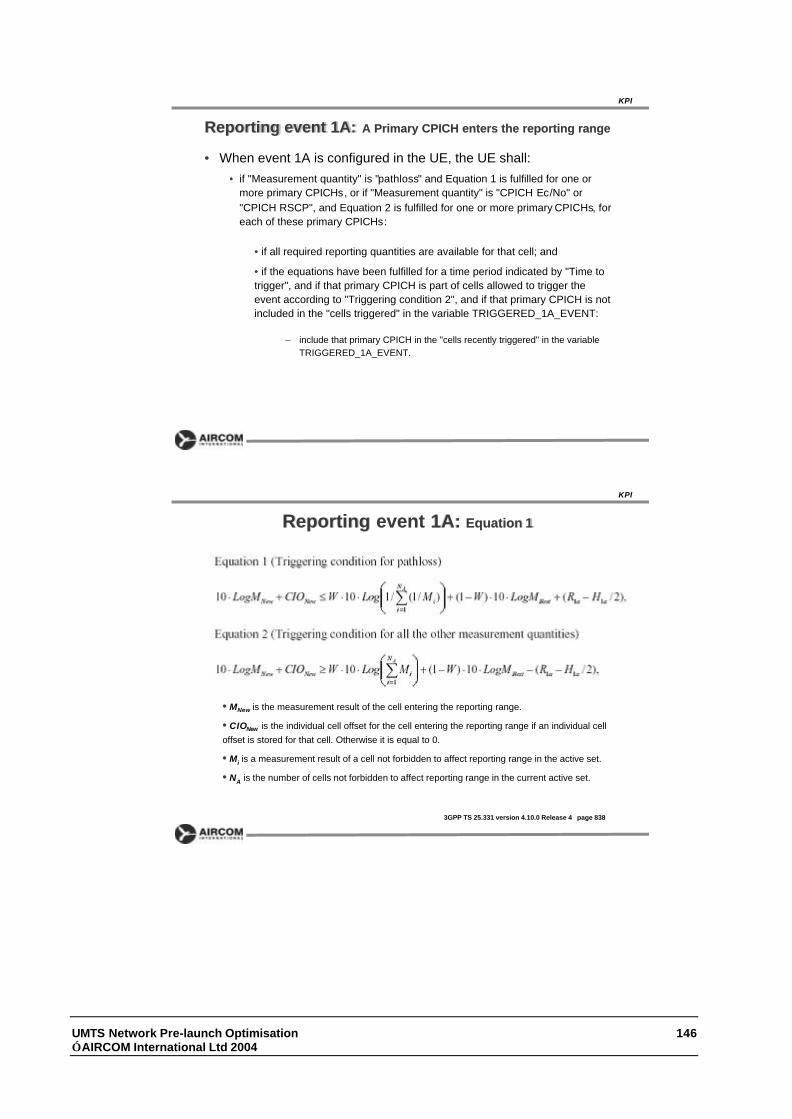
UMTS Network Pre-launch Optimisation 146 AIRCOM International Ltd 2004
Reporting event 1A:Reporting event 1A: A Primary CPICH enters the reporting rangeA Primary CPICH enters the reporting range
• When event 1A is configured in the UE, the UE shall:• if "Measurement quantity" is "pathloss" and Equation 1 is fulfilled for one or
more primary CPICHs, or if "Measurement quantity" is "CPICH Ec/No" or"CPICH RSCP", and Equation 2 is fulfilled for one or more primary CPICHs, foreach of these primary CPICHs:
• if all required reporting quantities are available for that cell; and
• if the equations have been fulfilled for a time period indicated by "Time totrigger", and if that primary CPICH is part of cells allowed to trigger theevent according to "Triggering condition 2", and if that primary CPICH is notincluded in the "cells triggered" in the variable TRIGGERED_1A_EVENT:
– include that primary CPICH in the "cells recently triggered" in the variableTRIGGERED_1A_EVENT.
KPI
Reporting event 1A:Reporting event 1A: Equation 1Equation 1
KPI
• MNew is the measurement result of the cell entering the reporting range.
• CIONew is the individual cell offset for the cell entering the reporting range if an individual celloffset is stored for that cell. Otherwise it is equal to 0.
• Mi is a measurement result of a cell not forbidden to affect reporting range in the active set.
• NA is the number of cells not forbidden to affect reporting range in the current active set.
3GPP TS 25.331 version 4.10.0 Release 4 page 838

UMTS Network Pre-launch Optimisation 147 AIRCOM International Ltd 2004
Reporting event 1A:Reporting event 1A: Equation 1Equation 1
KPI
• For pathloss
• MBest is the measurement result of the cell
• For other measurements quantities.
• W is a parameter sent from UTRAN to UE.
• R1a is the reporting range constant.
• H1a is the hysteresis parameter for the event 1a.
• If the measurement results are pathloss or CPICH Ec/No then MNew, Mi and
MBest are expressed as ratios.
• If the measurement result is CPICH-RSCP then MNew, Mi and MBest are
expressed in mW.
8.4 Identifying the cause It is easy to say that the causes of calls being dropped should be categorised but the only symptom that the drive test team will notice is that the call has been dropped or failed to connect. In order to gain an insight into the cause of failure, it is necessary to examine the communication between the UE and the network. These mostly fall under the name of “layer 3 messages”. Examples of the uses of such messages will be considered using examples of call drop events. It is useful to have some familiarity with the message flows and structures. Messages are passed to the UE in the form of “System Information Blocks” which fall into different categories. A list is included here. Of particular significance is System Information Block (SIB) 18 that provides information regarding the neighbour list. It would be expected that SIB 18 is sent to the UE following an update of the active set.

UMTS Network Pre-launch Optimisation 148 AIRCOM International Ltd 2004
System Information StructureSystem Information Structure
• Measurement data which can be recorded are in the form of message flows.
• These message flows indicate which blocks of information have beentransmitted and from which channel.
• Broadcast Information is organised into a structure
• Master Information Block MIB•Scheduling Block SB
• System Information Block SIB
System Info and Message Flows
SCHEDULING_BLOCK_1BCCH10:44:24.554RRCD
SYSTEM_INFORMATION_BCHBCCH_BCH10:44:24.504RRCD
SYSTEM_INFORMATION_BLOCK_TYPE_1BCCH10:44:24.454RRCD
MASTER_INFORMATION_BLOCKBCCH10:44:24.414RRCD
SYSTEM_INFORMATION_BCHBCCH_BCH10:44:24.384RRCD
System Information Blocks System Information Blocks SIB’sSIB’s• 18 SIB’s defined by ETSI TS 25.331 Release 4
• Type 1
• NAS system information as well as UE Timers and counters
• Type 2
• URA identity• Type 3
• Parameters for cell selection and re-selection
• Type 4
• Same as Type 3 but in connected mode• Type 5
• Parameters for configuration of common physical channels
• Type 6
• Same as Type 5 but in connected mode
System Info and Message Flows

UMTS Network Pre-launch Optimisation 149 AIRCOM International Ltd 2004
System Information Blocks System Information Blocks SIB’sSIB’s• 18 SIB’s defined by ETSI TS 25.331 Release 4
• Type 7
• Fast changing parameters for UL interference
• Type 8
• Only for FDD – static CPCH information to be used in the cell• Type 9
• Only for FDD -- CPCH information to be used in the cell
• Type 10
• Only FDD – Used by UE’s having their DCH controlled by aDRAC.
• DRAC
• Type 11• Contains measurement control information to be used in the cell
• Type 12
• Same as Type 11 but in connected mode
System Info and Message Flows
System Information Blocks System Information Blocks SIB’sSIB’s• 18 SIB’s defined by ETSI TS 25.331 Release 4
• Type 13
• Used for ANSI-41
• Type 14
• Only TDD• Type 15
• UE positioning method for example GPS
• Type 16
• Radio bearer, transport channel and physical channelparameters to be stored by UE for use during Handover HO
• Type 17
• Only TDD• Type 18
• Contains PLMN identities of neighbouring cells
System Info and Message Flows

UMTS Network Pre-launch Optimisation 150 AIRCOM International Ltd 2004
Example 3g Message FlowExample 3g Message Flow
• Exercise• Check the SIB’s with the descriptions in the ETSI TS 25.331 document
SYSTEM_INFORMATION_BCHBCCH_BCH10:44:25.035RRCD
SYSTEM_INFORMATION_BCHBCCH_BCH10:44:24.985RRCD
SYSTEM_INFORMATION_BCHBCCH_BCH10:44:24.935RRCD
SYSTEM_INFORMATION_BLOCK_TYPE_18BCCH10:44:24.885RRCD
SYSTEM_INFORMATION_BLOCK_TYPE_7BCCH10:44:24.855RRCD
SYSTEM_INFORMATION_BLOCK_TYPE_3BCCH10:44:24.825RRCD
SYSTEM_INFORMATION_BLOCK_TYPE_2BCCH10:44:24.795RRCD
SYSTEM_INFORMATION_BCHBCCH_BCH10:44:24.775RRCD
SYSTEM_INFORMATION_BLOCK_TYPE_1BCCH10:44:24.725RRCD
MASTER_INFORMATION_BLOCKBCCH10:44:24.675RRCD
System Info and Message Flows
Example 3g Message FlowExample 3g Message Flow
• In this segment a call is established• Check the SIB’s with the descriptions in the ETSI TS 25.331 document
RADIO_BEARER_SETUP_COMPLETEDCCH10:36:31.444RRCU
RADIO_BEARER_SETUPDCCH10:36:30.733RRCD
DOWNLINK_DIRECT_TRANSFERDCCH10:36:30.162RRCD
CALL_PROCEEDINGDCCH10:36:30.162L3D
UPLINK_DIRECT_TRANSFERDCCH10:36:29.862RRCU
SETUPDCCH10:36:29.862L3U
DOWNLINK_DIRECT_TRANSFERDCCH10:36:29.842RRCD
CM_SERVICE_ACCEPTDCCH10:36:29.842L3D
INITIAL_DIRECT_TRANSFERDCCH10:36:29.531RRCU
CM_SERVICE_REQUESTDCCH10:36:29.531L3U
DCCH_RRC_CONNECTION_SETUP_COMPLETEDCCH10:36:29.461RRCU
RRC_CONNECTION_SETUPCCCH10:36:28.660RRCD
RRC_CONNECTION_REQUESTCCCH10:36:28.320RRCU
System Info and Message Flows

UMTS Network Pre-launch Optimisation 151 AIRCOM International Ltd 2004
Example 3g Message FlowExample 3g Message Flow
• During Call is message flow is repeated over and over
MEASUREMENT_CONTROLDCCH10:38:49.403RRCD
ACTIVE_SET_UPDATE_COMPLETEDCCH10:38:48.932RRCU
ACTIVE_SET_UPDATEDCCH10:38:48.922RRCD
MEASUREMENT_REPORTDCCH10:38:48.651RRCU
RRC_CONNECTION_RELEASE_COMPLETEDCCH10:44:24.034RRCU
RRC_CONNECTION_RELEASE_COMPLETEDCCH10:44:23.884RRCU
RRC_CONNECTION_RELEASE_COMPLETEDCCH10:44:23.753RRCU
RRC_CONNECTION_RELEASEDCCH10:44:23.713RRCD
UPLINK_DIRECT_TRANSFERDCCH10:44:23.433RRCU
IMSI_DETACH_INDICATIONDCCH10:44:23.433L3U
• Call detach sequence
System Info and Message Flows
8.4.1 Example 1: Examining measurement reports
In this scenario a call is dropped whilst moving along a road. Measurement reports can be displayed so that the experience of the mobile can be monitored is viewed. In this case the measurement reports revealed:
• Pilot dropping to –115 dBm
• Ec/Io dropping to –20 dB
• BLER rising to very high percentages
The call dropped due to a “poor RF environment”. It can be argued that this “should not happen” if the physical aspects have been optimised. However, we only work to a 95% probability in the hope that this will lead to an acceptable experience on the ground. The hope is that the 5% not covered will not be too important. Drive testing can be regarded as a method of highlighting areas where this is not the case. However, the UE measurements should be compared with scanner data for the same location. A discrepancy should be expected because:
• The UE antenna may be inside the vehicle whereas the scanner antenna is roof-mounted.

UMTS Network Pre-launch Optimisation 152 AIRCOM International Ltd 2004
• The UE is not a calibrated measurement device.
One other question that must be asked is whether the UE and the scanner agree on the “best pilot”. In other words was the scanner measuring a pilot signal that was not recorded at all by the UE? This could reveal a neighbour list problem whereby the best server never became a member of the active set. One further possibility is that the UE itself is not of a good specification. Perhaps a different UE would not drop the call under the same circumstances. If all these possible reasons have been eliminated, then it is necessary to examine ways of improving the network coverage in order to prevent calls being dropped at this particular location.
8.4.2 Example 2: Examining active set update reports
In this example a call is dropped in an area where coverage is very good but Ec/Io drops to very low levels. It was found to be due to a combination of unusual propagation mechanisms and a less than ideal neighbour lists. It involves three cells (cell 1, cell 2 and cell 3). The location of the area concerned was expected to have cell 1 as the best server. Cell 2 would have been a significant neighbour and was on the neighbour list. Cell 3 also had a low path loss to that area and was a listed neighbour. However, due to some local shadowing effects, Cell 2 became primary server and, in fact, Cell 1 was dropped from the active set because the pilot strength dropped below the soft hand over margin. Now, Cell 3 was not on the neighbour list of Cell 2 but, due to near line of sight existing to Cell 3 from a small part of this area, it was received at a high level. Because it is not on the neighbour list, this represented interference and was at a strong enough level to cause a call drop. Solutions to this happened in two stages:
• The quick fix was to add Cell 3 to the neighbour list of Cell 2. This resulted in Cell 3 being on the monitored list and hence could join the active set when appropriate.
• The long-term solution was to control the radiation from Cell 3 in order that it only provided coverage where required and did not cause undue interference in other locations.
8.4.3 Example 3: Sudden increase in interference
When drive test measurements report levels of Ec/Io, the default is that this refers to the best server. There are circumstances when this is not a good representation of the experience of the UE. Calls can drop where there is a sudden change in the signal strengths from cells. Consider the situation where a UE travels at significant speed around a corner in an urban environment. Suppose it moves rapidly from a location where “cell

UMTS Network Pre-launch Optimisation 153 AIRCOM International Ltd 2004
1” is 15 dB stronger than “cell 2” to a location where the reverse is true. If this transition occurs before cell 2 can be added to the active set and become the primary server, then it is possible for the call to drop. UEs must spend sufficient time in the transition region for hand over to occur. At road junctions, radiation from cells should not simply “shoot across” the junction. The situation is potentially worse when the cell is at street level. If the cell is above roof top level then the signal will tend to penetrate further and reduce in strength less rapidly.
The Analysis Engineer will be alerted to the existence of such problems by call drops being reported at these locations. The UE reports will show the Ec/Io at a very bad level immediately before drop. After dropping the call the UE will re-connect with the network. In this example the re-connection will be on the new cell and the Ec/Io reported now will be remarkably good. Scanner data monitoring the strengths of different pilots can be used to support the reasoning.
Functional TestingFunctional Testing
Functional Testing
• Whilst drive testing and measuring pilot strengths, it isusual to monitor call success.
• Calls are usually one of three types;• voice (“AMR”)
• video telephony (“VT”)
• packet traffic (“http” or “ftp”)
• AMR or VT testing can be one of two types• “drive till drop”
• cyclic call attempts (e.g. 2 minute cycle)
• packet traffic involves downloading data of varying sizes.

UMTS Network Pre-launch Optimisation 154 AIRCOM International Ltd 2004
Functional Testing - measurementsFunctional Testing - measurements
Functional Testing
• When carrying out cyclic testing with AMR or VT the CallCompletion Success Rate (CCSR) is the most significantparameter.
• When testing packet traffic, the Context ActivationSuccess Rate (CASR) and the throughput/time todownload are of great interest.
• Agreement must be made on suitable timeouts: e.g. howlong should the UE attempt to establish a call (20seconds?) before a failure is registered. Likewise forcontext activation.
• Driving till drop checks for continuous coveragerequirements, neighbour planning and hand overprocedures.
Functional Testing - using resultsFunctional Testing - using results
Functional Testing
• In the period before the physical environment has besatisfactorily optimised, functional tests are of interest toindicate that the network is functioning properly and willindicate events such as “sleeping cells”.
• However, not every call drop will be investigated as it isknown that there are gaps in coverage and/or areas ofhigh interference.
• Once the physical environment has been optimised, thefunctional test results become very significant andprovide the final verdict on the whole optimisationprocess.

UMTS Network Pre-launch Optimisation 155 AIRCOM International Ltd 2004
Functional Testing - approachFunctional Testing - approach
Functional Testing
• It must be accepted and anticipated that the functionaltesting will not reveal perfect results. Calls will still dropor fail to set up.
• Failures can fall into one of several categories• Coverage or interference problems
• Hand over failure
• Network problem
• Handset issue
Coverage/Interference ProblemsCoverage/Interference Problems
Functional Testing
• Remember we would to thresholds at 95% probability -not 100%.
• Hope is that the 5% of problem areas will not be critical.
• A call drop due to coverage and/or interference problemindicates that air interface is of poor quality in animportant area. This should be addressed.
• Note that all RF measurements have been performed onthe downlink. An uplink problem should be investigatedif the downlink looks OK. E.g. is the cell receiver andmast head amplifier functioning satisfactorily. It ispossible to monitor the UE Tx power (e.g. >11 dBmindicates potential problem).
UMTS Network Pre-launch Optimisation 156 AIRCOM International Ltd 2004
Hand over problemsHand over problems
Functional Testing
• Perhaps neighbour list is not properly optimised.
• Remember that hand over requires a number ofsophisticated operations to be successfully carried out.
• Hand over is time dynamic. Not only do conditions haveto be right for HO, they have to be right for a sufficienttime for active set updates to occur.
• E.g. if there is only one cell in the active set, if this levelsuddenly drops before update can occur, the call mightdrop. UE speed may affect success rate.
• Truly optimising HO region extremely time-consuming:pre-launch best to concentrate on problem areas.
• Corrections can include parameters such as HO marginin addition to physical changes.
Network ProblemsNetwork Problems
Functional Testing
• Call can drop due to spurious messages going betweenthe UE and the Network.
• Additionally, some cells may be inactive (“sleeping”).
• Instances must be recorded and reported.
UMTS Network Pre-launch Optimisation 157 AIRCOM International Ltd 2004
Handset issuesHandset issues
Functional Testing
• On some occasions failure may be specific to a handset.
• Perhaps the handset does not respond to a pagingcommand or other message.
• Perhaps the handset drops a call in an environmentwhere other handsets do not drop calls.
• UMTS technology is still improving.
Identifying the CauseIdentifying the Cause
Functional Testing
• In order to gain an insight into the likely cause of calldrop, it is important to examine the communicationbetween the UE and the network.
• These are generally known as “layer 3 messages”.
• Two call drop examples are explained.

UMTS Network Pre-launch Optimisation 158 AIRCOM International Ltd 2004
Example 1: measurement reportsExample 1: measurement reports
Functional Testing
• Measurements reported by the UE show:• Pilot dropping to -115 dBm
• Ec/Io dropping to -20 dB
• BLER rising to very high levels
• Diagnosis is a straightforward “poor coverage” situation.
• Detailed investigation reveals that an additional site islikely to be required.
• Further questions:• does scanner agree with poor coverage diagnosis?
• What differences should be expected between scanner and UEmeasurements?
Example 1: measurement reportsExample 1: measurement reports
Functional Testing
• Difference between scanner and UE measurements canbe as large as 20 dB for certain vehicle configurations.
• UE antenna is in the vehicle, scanner antenna is roof-mounted.
• You must be “comfortable” that the difference isappropriate for the test you are making:
• Should interior of vehicle simulate significant (comparable to in-building) penetration losses?
• Is the UE measurement reliable - e.g. is it measuring the samepilot as the scanner?

UMTS Network Pre-launch Optimisation 159 AIRCOM International Ltd 2004
Example 2: AS update reportsExample 2: AS update reports
Functional Testing
• Another call drop occurred where the coverage in theform of pilot strength was good.
• AS update reports reveal an interesting sequence ofevents.
•Cell 1: expected primary server •Cell 2: Ncell to cell 1
•Cell 3: Ncell to cell 1
•Location of call drop
Example 2: AS update reportsExample 2: AS update reports
Functional Testing
• Due to shadowing effects, the following sequence tookplace.
•Cell 1: expected primary server •Cell 2:
•Cell 3: Ncell to cell 1
•Location of call drop
• Cell 2 became bestserver.
• Cell 1 drops fromactive set.
• Signal from Cell 3rises (not on Ncelllist for cell 2)causing poor Ec/Io.
• Call drops due tolow Ec/Io.

UMTS Network Pre-launch Optimisation 160 AIRCOM International Ltd 2004
Example 2: AS update reportsExample 2: AS update reports
Functional Testing
• Solutions:• Quick fix:
• add Cell 3 to Ncell list for Cell 2.
• Longer term:
• investigate radiation from Cell 3. It is a distant cell and isnot expected to become a member of the active set in thearea in question.
• Radiation from Cell 3 should be controlled, probably bydown-tilting but giving due regard to its required coveragearea.
Example 3: Sudden Change in SignalExample 3: Sudden Change in SignalStrengthStrength
Functional Testing
• Drive test reportsEc/Io for “bestserver”.
• Transition regionsbetween coverageareas can be small,particularly in urbanenvironments.
• If UE moves rapidlythrough such anarea, call can drop.
Cell 1
Cell 2
Cell 1 is 15dB strongerthan Cell 2
Cell 2 is 15dB strongerthan Cell 1

UMTS Network Pre-launch Optimisation 161 AIRCOM International Ltd 2004
Example 3: Sudden Change in SignalExample 3: Sudden Change in SignalStrengthStrength
Functional Testing
• For a successfulhand over, thesignals received bythe UE should riseand fall at a rate sothat the UE canexecute thenecessary active setupdates.
time
time
Signalstrength transition
transition
•Successful HO
•Call drop
Example 3: Sudden Change in SignalExample 3: Sudden Change in SignalStrengthStrength
Functional Testing
• Transition regionmust be largeenough to allowactive set update tooccur before UE isoverwhelmed byinterference.
Cell 1
Cell 2
TransitionRegion

UMTS Network Pre-launch Optimisation 162 AIRCOM International Ltd 2004
Example 3: Sudden Change in SignalExample 3: Sudden Change in SignalStrengthStrength
Functional Testing
• This can bealleviated by:
• providing a separatecell at theintersection
Cell 1
Cell 2
Example 3: Sudden Change in SignalExample 3: Sudden Change in SignalStrengthStrength
Functional Testing
• This can bealleviated by:
• providing a separatecell at theintersection
• placing cells abovestreet level toachieve greaterpenetration
Cell 2

UMTS Network Pre-launch Optimisation 163 AIRCOM International Ltd 2004
Example 3: Sudden Change in SignalExample 3: Sudden Change in SignalStrengthStrength
Functional Testing
• Detecting the problem:
• The Analysis Engineer will notice call drops• Investigation reveals that the UE reports very poor Ec/Io
immediately before it drops
• Once in idle mode the UE re-connects onto the new cell.
• The Ec/Io reported will be very good.• This large difference in Ec/Io indicates that the problem falls into
this category
• Scanner data showing pilot levels from the two cells will supportthe reasoning.


UMTS Network Pre-launch Optimisation 165 AIRCOM International Ltd 2004
add an appropriate margin, knowing the propagation exponent and the standard deviation of shadow fading. This will then allow a target path loss to be determined whereby the probability of the actual path loss being sufficiently low to allow a connection to be made is equal to the required probability. However, in UMTS systems the phenomenon of Noise Rise will affect the link budget. It is normal to add a Noise Rise (or “interference”) margin into the link budget. It is also usual to set this to the limit for a particular cell. This means that the calculations made will result in a path loss being output that will give a 90% connection (uplink Eb/No) probability even if the cell is fully loaded. At lower loading levels the probability will be greater. Thus, if an average probability is required, a lower value of Noise Rise should be used. This value of Noise Rise could be equal to that produced under “average” rather than “peak” loading conditions. The difference that this will produce will again depend on the desired capacity of the cell. The table shows the difference between peak and average Noise Rise and, further, provides an estimate in the difference this would make in the estimate of coverage area.
Peak Noise Rise Average Noise Rise % coverage area difference 2 dB 1.3 dB 9% 5 dB 3.4 dB 19% 10 dB 5.8 dB 43%
Assumptions: NR caused by voice traffic on cell with pole capacity of 65 connections. Cell provisioned for average traffic on a 2% blocking probability. Propagation exponent assumed to be 3.5.
Cl


UMTS Advanced Cell Planning and Optimisation 167 AIRCOM International Ltd 2003
9 Summarising Case Study
9.1 Introduction Now that we have assembled a useful “toolkit of knowledge” and discussed various techniques involved in advanced planning methods and optimisation procedures, it is possible to put ourselves in a “real world” situation and demonstrate our capabilities. The advanced network planner and optimiser should be able to demonstrate analytical and problem solving capabilities for a UMTS network. Problem areas can be identified and remedies recommended. As a starting point we will consider the situation where a UMTS network has been constructed and is active. Further we shall assume that it is not optimised. Problems with the network may fall into a number of categories
• Calls dropped • No coverage • Poor capacity • Slow download times
Any problems reported by customers or by network monitoring procedures should be analysed to see whether optimisation procedures can help the situation as opposed to simply investing heavily in more infrastructure. Rather than wait for complaints about network performance to arrive, the optimisation engineer should be able to identify problem areas, explain why they are likely to be problem areas and identify possible solutions. Drive test measurements are going to be valuable in this activity and should be used in conjunction with a planning tool.
9.2 The initial situation We shall assume that:

UMTS Network Pre-launch Optimisation 168 AIRCOM International Ltd 2004
• We have a network • It has not been optimised • We need to assess the quality of the network in an efficient manner and
report back. • The report should be able to predict areas where coverage and congestion
problems are going to occur.
9.3 Making the measurements Drive test measurements are going to be made using a proprietary scanner or test mobile. These will be able to provide a great deal of data. Initially, it is important to focus on a few, highly relevant parameters. A scanner will report on pilot strength (Ec) and also pilot Ec/No (although the value of No depend partly on the quality of the receiver itself). A test mobile will additionally be able to access the network and report on uplink transmit power. These measurements alone are sufficient to be able to comment on:
1. Coverage 2. Interference 3. DL capacity
9.4 Analysing Measurements
9.4.1 Coverage Pilot strength alone is a good indicator of basic coverage. As well as indicating whether the pilot is strong enough for a typical mobile to synchronise with, pilot strength indicates the path loss. This in turn can be used to predict uplink coverage. As an example consider a service for which the required Eb/No value is 5 dB. If it assumed that: Cell pilot strength = 33 dBm Noise Figure of Cell Receiver = 4 dB then the pilot strength can be used to indicate the throughput possible for a given noise rise limit (NR dB). Maximum link loss (UL) = 108 – 4 -5 + 10log(3840/bitrate) – NR. Thus at bit rate of 12.2 kbit/s and a noise rise limit of 3 dB, the maximum link loss is 121 dB. If the pilot strength is 33 dBm, this area is indicated by a pilot strength of -108 dBm. In practice a margin for fading would be expected and a minimum level of approximately -102 dBm would be sought. This policy of applying margins is very necessary if the drive testing is carried out exclusively out of doors and indoor coverage is required. Further, higher resource bearers cannot sustain as high a path loss as voice and a stronger pilot would be required to indicate uplink coverage. A typical set of thresholds would be

UMTS Advanced Cell Planning and Optimisation 169 AIRCOM International Ltd 2003
Service Required Pilot Strength Outdoor Voice -102 dBm In Car Voice -88 dBm Indoor Voice -80 dBm Indoor HSD -76 dBm
Things to check: are the assumptions made correct?
• Noise Rise Limit • Noise Figure of Cell Receiver (MHA can affect this) • Pilot Strength
9.4.1.1 Using uplink measurements Although, if the cell parameters are known accurately, reliable predictions of uplink coverage can be obtained from downlink measurements, it is desirable to have measurements of uplink transmit power for a particular service so that a check can be made on the coverage provided on the uplink. This is because using only downlink measurements relies on assumptions for the uplink Eb/No and interference levels to be assessed. Using a test mobile and monitoring the uplink transmit power will automatically take into account the effect of a rise in the target Eb/No due to adverse propagation conditions or extra power being required because of the presence of uplink interferfence. However, it must be borne in mind that the uplink might not be experiencing uplink noise rise at the designed level thus giving mobile power levels that are “kind”. If the network is quiet, the uplink noise rise will be very low. More realistic values of required uplink transmit power will be obtained if the noise level at the cell is raised artificially. This can be achieved by raising the effective noise figure of the cell (TRX) receiver. This can be done by inserting an attenuator before the receiver. Care must be taken if a MHA is used to place the attenuator before the MHA rather than between the MHA and the TRX receiver. It is likely that the measurements will be made as a result of drive tests undertaken outdoors. As with the downlink measurements, appropriate margins must be added for penetration loss and increased levels of shadow fading.
9.4.2 Interference
Pilot Strength alone is not a sufficient indicator of pilot coverage. The pilot channel is vital for cell selection, channel sounding and synchronisation purposes. The “pilot SIR” ratio must be above -15 dB. Unfortunately pilot SIR is not measured directly. Further it is very dependent on the loading levels on the downlink, and also on the quality of the UE receiver (its noise figure). However, the measurements made can be used to estimate whether the pilot SIR will be sufficiently high for detection purposes. The scanner will not report only on the best (or strongest) pilot but will report on all detectable pilots. This information, combined with some assumptions, can be used to estimate the pilot SIR at different locations. As an example, let us consider the situation where four pilots have been detected.
Pilot 1 -80 dBm

UMTS Network Pre-launch Optimisation 170 AIRCOM International Ltd 2004
Pilot 2 -84 dBm Pilot 3 -87 dBm Pilot 4 -90 dBm
In order to estimate the quality of the pilot, it is necessary to estimate the total effective level of noise plus interference. This must be done by considering conditions of heavy loading. It is possible to artificially load the downlink but this is not absolutely necessary. If we regard the -80 dBm pilot as the serving pilot, we need to make an assumption regarding the maximum downlink power and the pilot levels. If the maximum total transmit power is 10 dB more than the pilot then the three measured interfering pilots can be regarded as carrying potential interference levels of -74 dBm, -77 dBm and -80 dBm respectively. Indeed, it can be expected that there will be -71 dBm of interfering power emanating from the serving cell, although orthogonality would be expected to reduce this to an effective level of -75 dBm. The thermal noise level, even for a poor quality receiver would not be expected to exceed -100 dBm (negligible in this case). If the effective levels of interference are added the result is a total effective interference power of -70 dBm. Thus a pilot SIR of -10 dB would be a reasonable estimate. Anything less than -12 dB should be regarded as a cause for concern. The pilot Ec/Io (which is measured) does not include orthogonality and, in fact, includes the wanted, “best”, pilot power within the overall level of Io. In the above case, the value of Ec/Io under fully loaded conditions would be -12 dB. The measured value is recorded as -5.7 dB suggesting that the downlink was not heavily loaded when the measurements were made. This fact must be considered when assessing the quality of the downlink. The above analysis, although not too onerous, is somewhat time-consuming. It is possible, with experience, to adopt an appropriate threshold level of Ec/Io with which to highlight problem areas on the downlink. It is clear that a low level of Ec/Io will be due to a combination of “low Ec” and/or “high Io”. “low Ec” problems are due to high path loss. “High Io” problems are due to a high number of pilot signals that are of nearly equal strength. It may be that a high number of detectable pilots (>4) is alone a sufficient indicator of potential problems with downlink interference. If it is seen to be a reliable indicator, this will speed up analysis considerably.
9.4.3 Downlink Capacity The interference levels experienced on the downlink are very dependent on the location of the mobile that is suffering from the interference. By measuring the levels of the pilot and considering the cell parameters, it is possible to estimate important parameters:
• The capacity available if all cell power is devoted downloading data to users in that location.
• The throughput possible by devoting 1 watt of power to a user at that location.
• The power required for a particular throughput and Eb/No. It is reasonable to assume that the above details should relate to the situation where the network is fully loaded. We have already seen that pilot strengths can be used to

UMTS Advanced Cell Planning and Optimisation 171 AIRCOM International Ltd 2003
predict the value of pilot SIR for the best server. Considering the situation described above where the pilot SIR was estimated to be -12 dB under heavily loaded conditions, we know that this will also be the SIR experienced by a traffic channel of the same power. Suppose this is 2 W. If the service to be sent over this bearer requires an Eb/No value of 4 dB, a processing gain of 16 dB will be needed and the throughput will be limited to 96 kbit/s. This bearer represents one eighth of the capacity of the cell (as there is a total maximum of 16 W available for downlink traffic). Thus the total capacity on the downlink would be estimated to be 772 kbit/s. A bearer with a power of 1 W could sustain a data rate of 48 kbit/s and if a particular service (for example, a 128 kbit/s videophone at an Eb/No of 3 dB) is known to be required, this can be calculated to be the equivalent of 2.1 times a 48 kbit/s 4 dB Eb/No service and therefore each require traffic channel power of 2.1 watts. These predictions serve to give a useful indication of the capacity of the downlink if all users were at the same location (the “hotspot” scenario). It will often be required to estimate the capacity of the downlink if the users are spread throughout the coverage area of a cell. In order to estimate this, measurements need to be taken for representative locations within the cell. Suppose for example, it was felt that radio conditions on the cell could be described by six representative measurements from which pilot SIR could be predicted. The cell’s capacity could then be predicted on the assumption that traffic was going to be loaded evenly in those representative locations. Suppose the representative locations have pilot SIR estimates as follows.
Location Pilot SIR A -12 dB B -8 dB C -6 dB D -10 dB E -2 dB F -9 dB
The method described previously can be used to calculate the amount of power required to download a bearer with a nominal 1 kbit/s at an Eb/No of 4 dB, assuming the pilot power to be 2 W.
Location Pilot SIR Power for 1kbit/s @ 4 dB
A -12 dB 20.7 mW B -8 dB 8.2 mW C -6 dB 5.2 mW D -10 dB 13.1 mW E -2 dB 2.07 mW F -9 dB 10.4 mW Total power required for 6 kbit/s 59.6 mW
The total power required of 59.6 mW for 6 kbit/s at an Eb/No of 4 dB suggests that the total cell power of 16 W could sustain 1.6 Mbit/s. Notice that this is significantly larger than the capacity of 772 kbit/s that was estimated to be the limit of throughput if all users were at location A.

UMTS Network Pre-launch Optimisation 172 AIRCOM International Ltd 2004
This analysis can be extended to variable weightings of traffic across the cell coverage area as the following example shows for the various relative weightings indicated.
Location Pilot SIR Power for 1kbit/s @ 4 dB
Weighting Throughput Power Required
A -12 dB 20.7 mW 4 4 kbit/s 82.8 mW B -8 dB 8.2 mW 2 2 kbit/s 16.4 mW C -6 dB 5.2 mW 3 3 kbit/s 15.6 mW D -10 dB 13.1 mW 1 1 kbit/s 13.1 mW E -2 dB 2.07 mW 1 1 kbit/s 2.07 mW F -9 dB 10.4 mW 3 3 kbit/s 31.2 mW Totals 14 kbit/s 161.2 mW
This suggests that the cell capacity when 16 W of traffic power is used would be 1.39 Mbit/s. Notice that the above weightings show the traffic to be concentrated where the interference is worst, hence the lower capacity prediction compared with the evenly loaded case. The next example shows the situation where the weighting is in favour of those cells that have the lowest interference.
Location Pilot SIR Power for 1kbit/s @ 4 dB
Weighting Throughput Power Required
A -12 dB 20.7 mW 1 1 kbit/s 20.7 mW B -8 dB 8.2 mW 3 3 kbit/s 24.6 mW C -6 dB 5.2 mW 3 3 kbit/s 15.6 mW D -10 dB 13.1 mW 1 1 kbit/s 13.1 mW E -2 dB 2.07 mW 4 4 kbit/s 8.3 mW F -9 dB 10.4 mW 2 2 kbit/s 20.8 mW Totals 14 kbit/s 103.1 mW
This suggests a total capacity of 2.18 Mbit/s. Notice how the capacity is much greater. The benefit of ensuring that your areas of highest demand experience the lowest interference is clear.
9.5 Taking corrective action Improving the interference situation is clearly a good thing. In areas where a cell does not make a positive contribution to the performance of the network (by potentially being the best server) it is important that the link loss is maximised. It should be noted that this will benefit the uplink and downlink performance. In a network, it is inevitable that there are locations where near-equal signals from three cells on the macro-cell layer are received.
• Network performance can be improved by ensuring that these locations are away from predicted hotspots.
• Particular attention should be paid to locations where near-equal signals from more than three cells are required. One of the cells concerned is probably detrimental to network performance.

UMTS Advanced Cell Planning and Optimisation 173 AIRCOM International Ltd 2003
SummarisingSummarising Case Study Case Study• We have put together a useful “tool kit” of knowledge
• Further, we have examined examples of drive test data
• We should be able to analyse such drive test data and
•Predict network performance
•Identify problem areas
•Suggest corrective action
• When analysing such data we should think terms of
•Coverage
•Interference
•Capacity
Summarising Case Study
SummarisingSummarising Case Study Case Study
• Our Starting Point
•We have an active network.
•The network has not beenoptimised.
•Problems experiencedinclude:
– Calls dropped– No coverage– Low capacity– Slow download rates.
• We need to rectify theseproblems efficiently.
Summarising Case Study
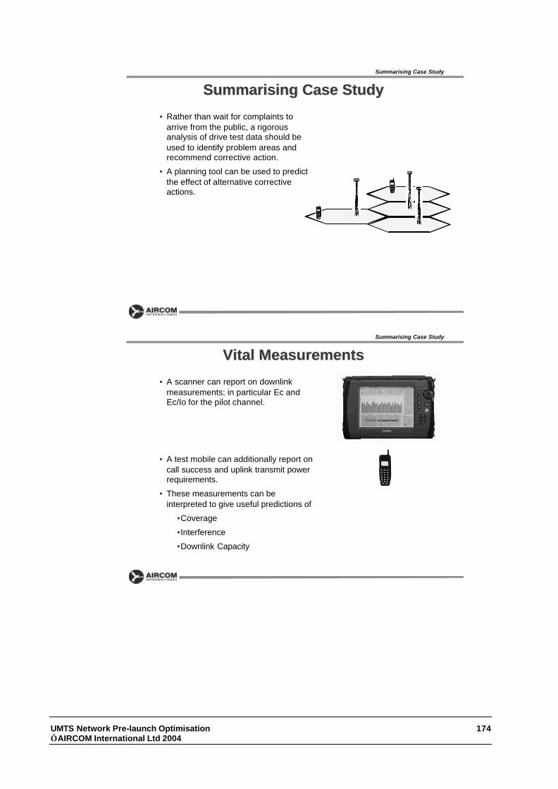
UMTS Network Pre-launch Optimisation 174 AIRCOM International Ltd 2004
SummarisingSummarising Case Study Case Study
• Rather than wait for complaints toarrive from the public, a rigorousanalysis of drive test data should beused to identify problem areas andrecommend corrective action.
• A planning tool can be used to predictthe effect of alternative correctiveactions.
Summarising Case Study
Vital MeasurementsVital Measurements
• A scanner can report on downlinkmeasurements; in particular Ec andEc/Io for the pilot channel.
• A test mobile can additionally report oncall success and uplink transmit powerrequirements.
• These measurements can beinterpreted to give useful predictions of
•Coverage
•Interference
•Downlink Capacity
Summarising Case Study

UMTS Advanced Cell Planning and Optimisation 175 AIRCOM International Ltd 2003
Using Pilot Strength to predict CoverageUsing Pilot Strength to predict Coverage• Measurements of pilot strength can be a very useful predictor of uplink
coverage.
• Other parameters need to be known:
•Tx Pilot Power
•NR limit and Noise Floor of cell.
•Bit rate and Eb/No of service for which coverage is being predicted.
Summarising Case Study
Using Pilot Strength to predict CoverageUsing Pilot Strength to predict Coverage• For example;
•NR limit set to 3 dB; Noise Floor of Cell = -104 dBm
•Eb/No required = 5 dB; bitrate = 12200 bits per second
•Pilot Power = 33 dBm
•Maximum mobile power = 21 dBm
Summarising Case Study
• Calculations;
•Processing Gain = 25 dB; Required SNR = -20 dB
•Maximum Noise Floor = -101 dBm
• Required Signal Strength = -121 dBm
•Maximum link loss = 142 dB
•Pilot Strength = -109 dBm

UMTS Network Pre-launch Optimisation 176 AIRCOM International Ltd 2004
Using Pilot Strength to predict Coverage -Using Pilot Strength to predict Coverage -marginsmargins
• If =-109 dBm was actually measured, coverage could not be confidentlyassumed.
• Margins would be required.
• This is especially true if measurements were made out of doors toindicate indoor coverage.
• The margins required depend on the characteristics of the buildings inquestion.
•Typical required minimum values:– Outdoor: -105 dBm– In Car: -96 dBm– In Building: -86 dBm– HSD In Building: -80 dBm
• Note that these are measured values: not predicted.
• Predicted values must additionally consider errors in the path lossmodel.
Summarising Case Study
Predicting Coverage (continued) – the value ofPredicting Coverage (continued) – the value ofuplink (test mobile) measurements.uplink (test mobile) measurements.
• The prediction of coverage using pilot strength as an indicator madesome assumptions:
•Eb/No required.
•Uplink interference experienced.
• A record of the uplink power needed for a particular service willautomatically account for these factors.
• If a mobile has a maximum transmit power of +21 dBm then thefollowing conclusions can be drawn:
•Required Tx Power > 17 dBm: Coverage unreliable outdoors
•Required Tx Power > 8 dBm: Outdoor coverage only
•Required Tx Power > -2 dBm: In Car coverage
•Required Tx Power < -2 dBm: Indoor coverage
Summarising Case Study

UMTS Advanced Cell Planning and Optimisation 177 AIRCOM International Ltd 2003
Simulating the effect of UL Noise RiseSimulating the effect of UL Noise Rise
• If the network is“quiet” when thetests are conducted,the results will beoptimistic.
• A noise rise can besimulated byincreasing the NoiseFigure of the cellreceiver. This canbe achieved simplyby adding anattenuator in thefeeder.
Summarising Case Study
•TRx •TRx
I 3 dB
NF = 5 dB NF = 8 dB
Simulating the effect of UL Noise RiseSimulating the effect of UL Noise Rise
• If the cell has a MHAfitted, the attenuatormust be fitted abovethe MHA.
• Otherwise, the MHAwill reduce the effect ofthe attenuator.
Summarising Case Study
TRx TRx
I
3 dBI

UMTS Network Pre-launch Optimisation 178 AIRCOM International Ltd 2004
InterferenceInterference
• Pilot Strength alone isnot a sufficientindicator of pilotcoverage.
• The “Pilot SIR” mustbe better thanapproximately -15 dBfor the pilot to beusable.
Summarising Case Study
Interference – Pilot SIRInterference – Pilot SIR• The Interference + noise
experienced comes from:
•Other cells
•Thermal noise
•Other channels onown cell
– Note other channelson own cell willbenefit fromorthogonality.
• Measurements ofstrengths of all pilots canbe used.
Summarising Case Study

UMTS Advanced Cell Planning and Optimisation 179 AIRCOM International Ltd 2003
Interference – Deducing Pilot SIRInterference – Deducing Pilot SIR• Suppose 4 pilots
are detected:•-80 dBm (bestserver)
•-84 dBm
•-87 dBm
•-90 dBm
• Assume thermal noiseis at -100 dBm.
Summarising Case Study
Interference – Deducing Pilot SIRInterference – Deducing Pilot SIRSummarising Case Study
• When network is heavilyloaded interference fromown cell (assuming 43dBm max power and 33dBm pilot power) is at-71 dBm. Effect oforthogonality is to reducethis to -75 dBm [10log(1-0.6) = 4 dB].
• Other interferers are -74dBm; -77 dBm; -80 dBm.
• Total noise plusinterference = -70 dBm.
•Pilot Power = 33 dBm
•Maximum Power = 43 dBm

UMTS Network Pre-launch Optimisation 180 AIRCOM International Ltd 2004
Interference – Pilot SIRInterference – Pilot SIR• Pilot strength (best
server) = -80 dBm.
• Predicted “noise plusinterference” underconditions of heavy load= -70 dBm.
• Pilot SIR = -10 dB.
• Anything less than -12dB would cause concern.
• Note: it is important thatpredictions are made fora fully loaded downlink.
Summarising Case Study
Wanted Pilot = -80 dBm
Noise + Interference = -70 dBm
Pilot SIR = -10 dB
Interference – Pilot Ec/IoInterference – Pilot Ec/Io• Pilot SIR is not measured
– it must be deducedfrom pilot strengthmeasurements.
• Pilot Ec/Io can bemeasured.
• Note that no benefit fromorthogonality ismeasured and, also, the“wanted” pilot power isincluded in “Io”.
• Pilot SIR will be betterthan Ec/Io
Summarising Case Study
• High level of pilot Ec/Ioindicates lightly loadednetwork – values wouldbe much worse underheavy loading conditions.

UMTS Advanced Cell Planning and Optimisation 181 AIRCOM International Ltd 2003
Interference – Pilot Ec/IoInterference – Pilot Ec/Io
• Although an allowancemust be made foradditional downlinkinterference when anetwork is heavilyloaded, Ec/Io is a usefulindicator of the quality ofthe radio channel.
• A poor Ec/Io could bedue to “low Ec” or “highIo”.
Summarising Case Study
Interference – Predicting Downlink CapacityInterference – Predicting Downlink Capacity• Further calculations are possible:
•If 1 watt of power wasavailable for a downlinkbearer, this bearer would beable to sustain 76 kbit/s at 4dB Eb/No.
•A service with a 128 kbit/sthroughput at an Eb/No valueof 3 dB has a relativeamplitude of 1.33 comparedto the 76 kbit/s, 4 dB Eb/Noservice and would thereforerequire 1.33 watts of DLpower.
Summarising Case Study
Wanted Pilot = -80 dBm
Noise + Interference = -70 dBm
Pilot SIR = -10 dB

UMTS Network Pre-launch Optimisation 182 AIRCOM International Ltd 2004
Predicting Downlink Capacity – spread trafficPredicting Downlink Capacity – spread traffic
• These calculations are only validat one location. Supposemeasurements were made atdifferent locations within a cell.These allowed the followingestimates to be made for pilotSIR:
Summarising Case Study
-9 dBF-2 dBE-10 dBD-6 dBC-8 dBB-12 dBAPilot SIRLocation
Predicting Downlink Capacity – spread trafficPredicting Downlink Capacity – spread traffic
• The same method can be used to deduce the powerrequired for a nominal 1 kbit/s, 4 dB Eb/No bearer ateach location. The total power required for the totalthroughput can be used to estimate the DL capacity.
Summarising Case Study
59.6 mWTotal power required for 6 kbit/s10.4 mW-9 dBF2.07 mW-2 dBE13.1 mW-10 dBD5.2 mW-6 dBC8.2 mW-8 dBB20.7 mW-12 dBA
Power for 1kbit/s @4 dB
Pilot SIRLocation

UMTS Advanced Cell Planning and Optimisation 183 AIRCOM International Ltd 2003
Predicting Downlink Capacity – spread trafficPredicting Downlink Capacity – spread traffic
• 59.6 mW required for 6 kbit/s.
• 16 W would support 1611 kbit/s
• This is significantly larger than 1224 kbit/s if allexperienced a -10 dB pilot SIR.
Summarising Case Study
Predicting Downlink Capacity – unevenly spreadPredicting Downlink Capacity – unevenly spreadtraffictraffic
• The method can be extended to include relativeweightings of traffic density at particular points.
Summarising Case Study
161.2 mW14 kbit/sTotals
31.2 mW3 kbit/s310.4 mW-9 dBF
2.07 mW1 kbit/s12.07 mW-2 dBE
13.1 mW1 kbit/s113.1 mW-10 dBD
15.6 mW3 kbit/s35.2 mW-6 dBC
16.4 mW2 kbit/s28.2 mW-8 dBB
82.8 mW4 kbit/s420.7 mW-12 dBA
PowerRequired
Throughput
Weight-ing
Power for 1kbit/s@ 4 dB
Pilot SIRLocation

UMTS Network Pre-launch Optimisation 184 AIRCOM International Ltd 2004
Predicting Downlink Capacity – unevenly spreadPredicting Downlink Capacity – unevenly spreadtraffictraffic
• 161.1 mW for 14 kbit/s: 16 W would support 1390 kbit/swith these weightings.
Summarising Case Study
161.2 mW14 kbit/sTotals
31.2 mW3 kbit/s310.4 mW-9 dBF
2.07 mW1 kbit/s12.07 mW-2 dBE
13.1 mW1 kbit/s113.1 mW-10 dBD
15.6 mW3 kbit/s35.2 mW-6 dBC
16.4 mW2 kbit/s28.2 mW-8 dBB
82.8 mW4 kbit/s420.7 mW-12 dBA
PowerRequired
Throughput
Weight-ing
Power for 1kbit/s@ 4 dB
Pilot SIRLocation
Predicting Downlink Capacity – unevenly spreadPredicting Downlink Capacity – unevenly spreadtraffic: exercisetraffic: exercise
• Estimate the downlink capacity with these weightings.
Summarising Case Study
Totals
210.4 mW-9 dBF
42.07 mW-2 dBE
113.1 mW-10 dBD
35.2 mW-6 dBC
38.2 mW-8 dBB
120.7 mW-12 dBA
PowerRequired
Throughput
Weight-ing
Power for 1kbit/s@ 4 dB
Pilot SIRLocation

UMTS Advanced Cell Planning and Optimisation 185 AIRCOM International Ltd 2003
Taking Corrective ActionTaking Corrective Action
• Receiving “too many” pilotswith near-equal strength isan indicator of potentialinterference problems.
• A possible way how thiscould arise is described.
• Areas where there are 3near-equal pilots willinevitably occur.
• Suppose that the antennasare re-orientated toalleviate a coverageproblem.
Summarising Case Study
Coverage Gap
Taking Corrective ActionTaking Corrective Action
• Re-orientating theantennas will help to fill in acoverage gap.
• However a region hasemerged where five serverwould have near-equalpath loss.
• This would cause problemswith pilot detection andpoor achievable downlinkbitrates.
Summarising Case Study
DL Interference Problem

UMTS Network Pre-launch Optimisation 186 AIRCOM International Ltd 2004
Taking Corrective ActionTaking Corrective Action
• Corrective action wouldhave to involve providing adominant server in thearea.
• This would entaildowntilting antennas andperhaps having tocompromise on thecoverage in certain areas.
• A MHA or UL diversitysystem will help withcoverage.
Summarising Case Study
Re-orientate to provide
dominant server
Down-tilt here
Concluding RemarksConcluding Remarks
•Why are we bothering?
•To make or save money.
•How do operators make money?
•By transferring data from one point toanother
Network Implementation and Evolution

UMTS Advanced Cell Planning and Optimisation 187 AIRCOM International Ltd 2003
• Revenue Gains
•Suppose revenue of $ 0.1 is received for every megabit of
data transferred.
•A cell whose capacity is increased by 500 kbit/s (per
carrier) can be expected to earn approximately $ 200000
per carrier per year extra (depending on occupancy rates).
Concluding RemarksConcluding RemarksNetwork Implementation and Evolution
• Revenue Gains
•If an engineer takes responsibility for 60 cells, each with a
single carrier, the potential gains add up to $ 12 million per
engineer.
•Go and make an extra $ 12 million per year.
Concluding RemarksConcluding RemarksNetwork Implementation and Evolution