UML and SOA Overview with Example Applications to the xLPR ...

ORNL-2013/45084

UML and SOA Overview with Example

Applications to the xLPR V.2 Project

Prepared by

H. B. Klasky, P. T. Williams, and B. R. Bass

Oak Ridge National Laboratory

Prepared for

U.S. Nuclear Regulatory Commission

CAUTION

This document has not been given final patent

clearance and is for internal use only. If this

document is to be given public release, it must be

cleared through the site Technical Information

Office, which will see that the proper patent and

technical information reviews are completed in

accordance with the policies of Oak Ridge

National Laboratory and UT-Battelle, LLC.

This report was prepared as an account of work sponsored by an

agency of the United States government. Neither the United States

government nor any agency thereof, nor any of their employees,

makes any warranty, express or implied, or assumes any legal

liability or responsibility for the accuracy, completeness, or

usefulness of any information, apparatus, product, or process

disclosed, or represents that its use would not infringe privately

owned rights. Reference herein to any specific commercial product,

process, or service by trade name, trademark, manufacturer, or

otherwise, does not necessarily constitute or imply its endorsement,

recommendation, or favoring by the United States government or

any agency thereof. The views and opinions of authors expressed

herein do not necessarily state or reflect those of the United States

government or any agency thereof.

ORNL/TM-2013/45084

UML and SOA Overview with Example

Applications to the xLPR V.2 Project

Manuscript Completed: January 2012

Date Published: September 2013

Prepared by

H. B. Klasky, P. T. Williams and B. R. Bass


Managed by UT-Battelle, LLC


Oak Ridge, TN 37831-6085

for the

U.S. DEPARTMENT OF ENERGY

under contract DE-AC05-00OR22725

Prepared for

Division of Engineering

Office of Nuclear Regulatory Research

U.S. Nuclear Regulatory Commission

Washington, DC 20555-0001

NRC Job Code N6438

This page is intentionally left blank.

Table of Contents

Abstract .................................................................................................................................................. 1

1 Background on GoldSim External Functions ................................................................................ 2

2 UML Diagrams Relevant To xLPR Module Design ..................................................................... 4

2.1 What is the Unified Modeling Language or UML? ............................................................... 4

2.2 Component Diagram .............................................................................................................. 5

2.3 Deployment diagram .............................................................................................................. 6

2.4 Behavioral Modeling Diagrams ............................................................................................. 7

2.4.1 Activity diagram ............................................................................................................. 7

2.4.2 Sequence diagram ........................................................................................................... 8

2.4.3 Collaboration Diagram ................................................................................................... 9

2.4.4 Use case diagram .......................................................................................................... 10

2.4.5 State-chart Diagram ...................................................................................................... 11

2.4.6 Architectural Modeling Diagram .................................................................................. 11

2.5 Suggestions on Available UML Tools ................................................................................. 12

3 Service Oriented Architecture – Designing External Modules As Services ................................ 15

3.1 What is Service-Oriented Architecture or SOA? ................................................................. 15

3.2 SOA step by step .................................................................................................................. 16

3.2.1 Example 1: Model Simple Calculator .......................................................................... 17

4 Example of a SOA Module .......................................................................................................... 19

4.1.1 Example 2: Model Charpy Curve ................................................................................. 19

5 Summary And Conlusions ........................................................................................................... 28

6 UML GLOSSARY ...................................................................................................................... 29

6.1.1 UML Notations ............................................................................................................. 29

6.1.2 UML Diagrams ............................................................................................................. 40

References .............................................................................................................................................. 1

Table of Figures

Figure 1 Sample GS Design of External Functions ............................................................................... 3

Figure 2 Component Diagram................................................................................................................ 6

Figure 3 Deployment Diagram .............................................................................................................. 7

Figure 4 Activity Diagram ..................................................................................................................... 8

Figure 5 Sequence Diagram ................................................................................................................... 9

Figure 6 Collaboration Diagram .......................................................................................................... 10

Figure 7 Use Case Diagram ................................................................................................................. 10

Figure 8 State-chart Diagram ............................................................................................................... 11

Figure 9 Architectural Modeling Diagram ........................................................................................... 12

Figure 10 Class Notation ..................................................................................................................... 29

Figure 11 Class Notation Example. ..................................................................................................... 30

Figure 12 Object Notation ................................................................................................................... 30

Figure 13 Active Class Notation .......................................................................................................... 31

Figure 14 Interface Notation on UML 1.0 ........................................................................................... 31

Figure 15 Interface Notation on UML 2.0 ........................................................................................... 31

Figure 16 Collaboration Notation ........................................................................................................ 32

Figure 17 Use Case Notation ............................................................................................................... 32

Figure 18 Actor Notation ..................................................................................................................... 33

Figure 19 Initial State Notation ............................................................................................................ 33

Figure 20 Final State Notation ............................................................................................................. 33

Figure 21 Component Notation ........................................................................................................... 34

Figure 22 Node Notation ..................................................................................................................... 34

Figure 23 Interaction Notation ............................................................................................................. 34

Figure 24 Interaction Notation in a Sequence Diagram ....................................................................... 35

Figure 25 State Notation ...................................................................................................................... 35

Figure 26 State Machine Notation ....................................................................................................... 36

Figure 27 Package Notation Explained ................................................................................................ 36

Figure 28 Package Notation ................................................................................................................. 37

Figure 29 Note Notation Explained ..................................................................................................... 37

Figure 30 Note Notation ...................................................................................................................... 37

Figure 31 Dependency Notation .......................................................................................................... 38

Figure 32 Association Notation ........................................................................................................... 38

Figure 33 Generalization Notation Explained ...................................................................................... 39

Figure 34 Generalization Notation ....................................................................................................... 39

Figure 35 Realization Notation ............................................................................................................ 39

Figure 36 Extensibility Notation .......................................................................................................... 40

Figure 37 Class Diagram ...................................................................................................................... 41

Figure 38 Object Diagram .................................................................................................................... 42

ABSTRACT

This document provides guidance to xLPR model developers on how they can more effectively

design and communicate the requirements of their modules to the xLPR Computational Group (CG)

by using Unified Modeling Language (UML) and Service-Oriented Architectural (SOA) design

principles. This document gives an overview on the use of UML and SOA design principles to aid the

analysis, design and implementation of xLPR modules as GS external functions.

1 BACKGROUND ON GOLDSIM EXTERNAL FUNCTIONS

GoldSim allows the user to develop separate program modules [1] (written in C, C++, Pascal,

Fortran, or other compatible programming languages) which can then be directly coupled with the

main GoldSim algorithms. These user-defined modules are referred to as external functions, and are

linked into GoldSim as DLLs (Dynamic Link Libraries) at run time. Supporting both 32-bit and 64-

bit DLLs, GoldSim interfaces with the DLL via an External element.

From Appendix C in the GoldSim User’s Guide [1], external functions work with external elements

to do calculations or other manipulations that are not included in the standard capabilities of

GoldSim. The external function facility allows special purpose calculations or manipulations to be

accomplished with more flexibility, speed, or complexity than with the standard GoldSim element

types. These external functions are bound to the GoldSim executable code at run time using DLL

technology. The DLL files should be present in the same folder as the GoldSim.gsm file, in the same

folder as the GoldSim executable file, or elsewhere in the user’s path. Note that these functions are

external to GoldSim and are not covered by the standard GoldSim verification process. The user is

responsible for any necessary testing of external functions.

Every external function is called by GoldSim with specific requests. The requests include

initialization, returning the function version number, performing a normal calculation, and “cleaning

up” after a simulation. The function name and argument list (the set of input and output data for the

function) are specified by the GoldSim user when setting up the external element.

External functions should provide their own error handling, message handling, file management and

memory management if required. It is essential that when it receives a “clean up” request, an external

function should release any dynamically acquired memory and close any open files. In the case of an

error condition, the external function should always return an error code to GoldSim, so that the user

can be informed about the problem and the simulation can be terminated cleanly with no memory

leaks.

Figure 1 presents a sample of a GS diagram with external functions. Especifically, Figure 1 is a

diagram from “INPAGN_Laucher General Algorithm, Implementation and Execution of Probabilistic

Calculations Using GS” by D. Kalinich, P. Mattie, and C. Sallaberry from SNL, presentation on June

10, 2010; Rockville, MD.

xLPR modules are implemented as external functions in GoldSim.

Figure 1 Sample GS Design of External Functions

2 UML DIAGRAMS RELEVANT TO XLPR MODULE DESIGN

2.1 What is the Unified Modeling Language or UML?

From ref. [2], the Unified Modeling Language (UML) is the standard modeling language for software

and systems development. UML is a general-purpose notational language for specifying and

visualizing large complex software projects and can be thought of as a more powerful and more

general successor to the familiar software flowcharts used in the past. UML is very useful in

describing, designing, documenting, and managing the evolution of software. While there are a

number of ways of describing a model (including word descriptions, source code listings, tabulations

of input and outputs) to be implemented into a computational framework, the application of UML as a

communications tool between model developers and implementers has a number of advantages:

UML is a formal language – Each element of the language has a strongly defined meaning.

UML is concise – The entire language is made up of simple and straightforward notations.

UML is comprehensive – UML is capable of describing all important aspects of a software system at a

sufficiently high level of abstraction.

UML is scalable – Where needed, the language is formal enough to handle large system modeling

projects, but it also scales down to smaller elements.

UML is built on lessons learned – UML is the culmination of best practices developed over the last

20 years by the software community, where the ultimate technical imperative is the management of

complexity [3].

UML is a standard – UML is controlled by an open standards group with active contributions from a

worldwide group of software developers. The standard ensures UML’s transformability and

interoperability, i.e., developers are not tied to any one commercial UML tool or product.

UML was created by Object Management Group and UML 1.0 specification draft was proposed to

the OMG in January 1997. Since then, it has become the standard for building Object Oriented

Software. UML’s main versions since UML 1.0 are UML 1.5 and UML 2.0, the later was adopted on

2005

UML was developed to unify the notation of Object Oriented (OO) Languages. As most xLPR

modules have been written in Fortran, the OO Diagrams of UML will not apply to them. However,

the xLPR Developers can take advantage of the following diagrams which have a more general focus.

component diagrams,

deployment diagrams,

use case diagrams,

interaction diagrams

activity diagrams, and

state-chart diagrams.

The following sections present those diagrams.

2.2 Component Diagram

A component diagram represents a set of components and their relationships. Figure 2 shows a

sample component diagram.

Figure 2 Component Diagram

2.3 Deployment diagram

A deployment diagram represents a set of nodes and their relationships. Figure 3 shows a sample

deployment diagram.

Figure 3 Deployment Diagram

2.4 Behavioral Modeling Diagrams

Behavioral Modeling Diagrams represent interaction between elements of a system. They represent

activities, such as flow, communication, movement and change. UML behavioral modeling diagrams

are defined below.

2.4.1 Activity diagram

An activity diagram represents a series of functions that visualize the entire flow in a system during

execution. The flow can be sequential, concurrent or branched between the different components.

Figure 4 shows a sample activity diagram.

Figure 4 Activity Diagram

2.4.2 Sequence diagram

A sequence diagram represents sequential call flow from one element to another. Figure 5 shows a

sample sequence diagram.

Figure 5 Sequence Diagram

2.4.3 Collaboration Diagram

Collaboration diagram show communication between objects. It is similar to the sequence diagram,

with the added benefit that it shows the object organization. Figure 6 shows a sample collaboration

diagram.

Figure 6 Collaboration Diagram

2.4.4 Use case diagram

The use case represents a scenario of the system, i.e. they tell a story. In the scenario there are actors.

The use case diagram describes how actors relate or communicate with one another. Figure 7 shows a

sample use case diagram

Figure 7 Use Case Diagram

2.4.5 State-chart Diagram

The state-chart diagram represents the change of states in a component of a system. It also describes

the events that cause that change of states, which could be internal or external factors. Figure 8

presents a sample state-chart diagram.

Figure 8 State-chart Diagram

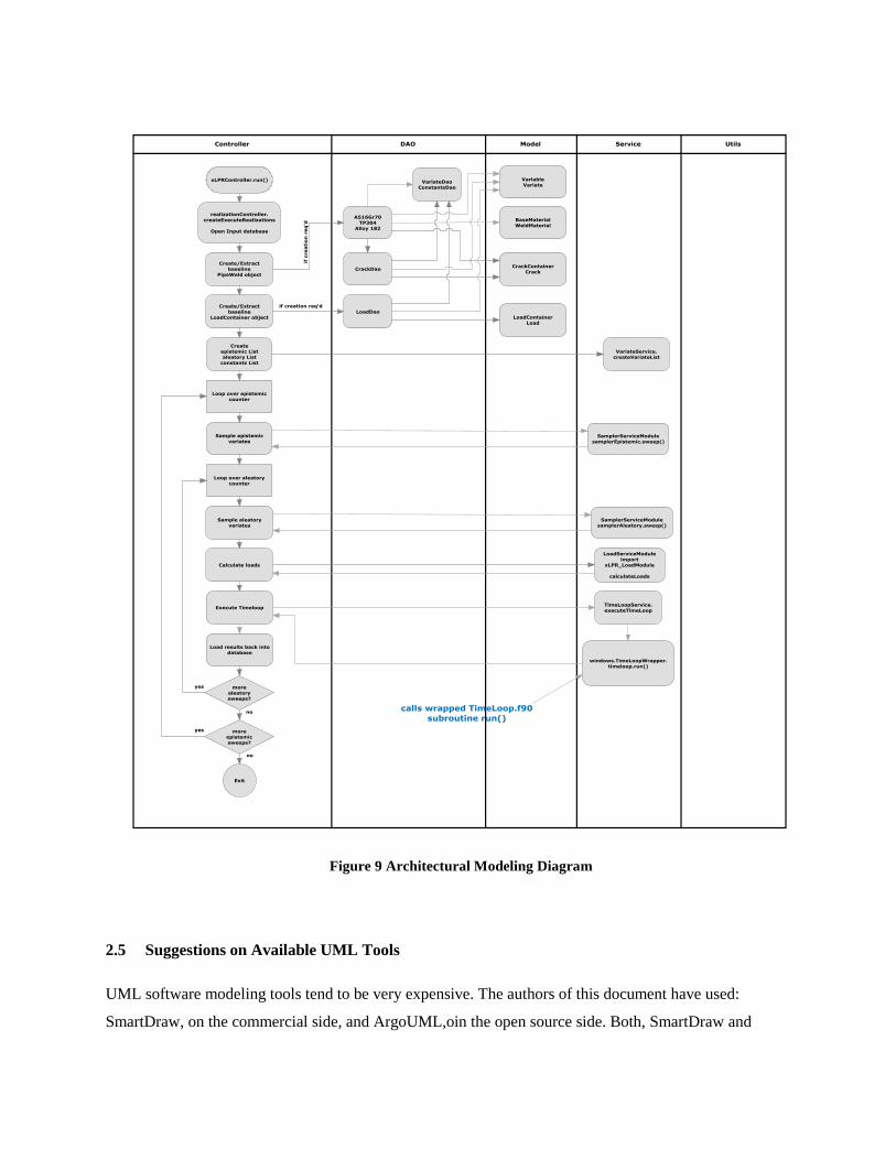
2.4.6 Architectural Modeling Diagram

The Architectural Modeling Diagram is a model that represents the overall framework of the system.

It contains both structural and behavioral elements. A sample Architectural Modeling Diagram is

shown on Figure 9.

2.5 Suggestions on Available UML Tools

UML software modeling tools tend to be very expensive. The authors of this document have used:

SmartDraw, on the commercial side, and ArgoUML,oin the open source side. Both, SmartDraw and

Figure 9 Architectural Modeling Diagram

ArgoUML, our experience with these tools was very good. However, any good text editor that allows

insertion of shapes, as MS Word, will be enough to help describing a system using UML notation.

.

3 SERVICE ORIENTED ARCHITECTURE – DESIGNING EXTERNAL MODULES AS

SERVICES

Some of the main advantages of Service oriented architecture (SOA) are reusability, maintainability

and scalability.

3.1 What is Service-Oriented Architecture or SOA?

SOA is an architecture for building applications as a set of loosely coupled black-box components

orchestrated to deliver a well-defined level of service by linking together processes. SOA is defined

by a set of principles and methodologies for designing and developing software in the form of

interoperable services. These services are well-defined functionalities that are built as software

components (discrete pieces of code and/or data structures) that can be reused for different purposes.

SOA design principles are used during the phases of systems development and integration. SOA can

be seen in a continuum, arising from older concepts of distributed computing and modular

programming.

SOA is a black-box component architecture. SOA deliberately hides complexity wherever

possible, and the idea of the black box is integral to SOA. The black box enables the reuse of existing

applications by adding a fairly simple adapter to them, no matter how they were built.

SOA components are loosely coupled. The term loosely coupled refers to how two components

interact within SOA. One component passes data to another component and makes a request. The

second component carries out the request and, if necessary, passes data back to the first. The

emphasis is on simplicity and autonomy. Each component offers a small range of simple services to

other components. A set of loosely coupled components does the same work that used to be done

inside tightly structured applications, but the components can be combined and recombined in myriad

ways.

SOA components are orchestrated to link together through processes to deliver a well-defined

level of service. SOA creates a simple arrangement of components that can, collectively, deliver a

very complex service. Simultaneously, SOA must provide acceptable service levels.

SOA adheres to the following three requirements:

1. Services must be safe. Safe means that the service itself is secure and doesn’t produce bugs

and problems into the organization

2. Services must be accurate. Accuracy means that the service itself executes the function it’s

designed to execute.

3. Services must be predictable. Predictable means that the service does what its’ expected to

do.

How services communicate with each other is responsibility of the integration framework where the

services reside. A framework works as a pipe through which data and instructions flow. A service (or

module or software component) connects to the framework and passes it a message by using a

specified format, along with the address of the software component that needs to receive the message.

The framework completes the job of getting the message from the sending component to the receiving

component.

SOA goes very well with the spiral and agile software development process approaches. SOA aims to

deliver incremental functionality in a system that is expected to be in constant evolution.

Don’t try to boil the ocean. Don’t attempt to do everything at once. Initially, prove

your success with SOA by starting with a project that is small, achievable in a short

time, and will have a significant impact — then build incrementally.

3.2 SOA step by step

In the following section, we have made an attempt to simply and describe the basic SOA principles.

These principles can be applied to defining, designing and implementing a Service following basic

SOA principles.

Code designers and programmers need to try to answer the steps below to defining, designing and

implementing their Module as a Service.

1. What does your model do?

2. Look for pre-integrated software components and pre-built reusable services that you can begin

using right away. If you find this, you may be able to just write a software layer on top to access a

well-tested module of software, otherwise, we will need to write our own.

3. Identify the functions that your model is going to provide to the framework or other modules.

4. Define an interface, i.e. a template that will serve as an index of the functions that your module

(service) is going to provide.

Comment: Leave the details of the implementation to lower level development, where greater

details will be introduced. Those details should not be exposed at the interface level.

5. For each function, identify inputs and outputs.

6. For each input, identify where should it come from and the data type expected

7. For each output, identify the resulting data type.

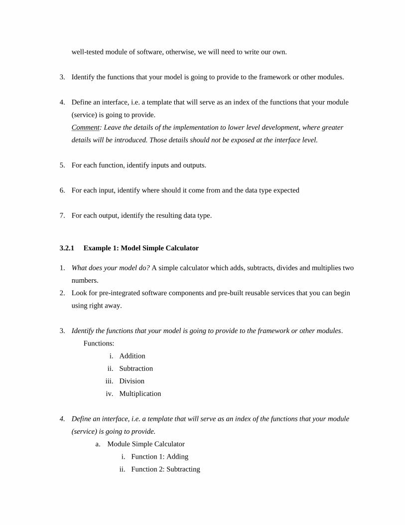
3.2.1 Example 1: Model Simple Calculator

1. What does your model do? A simple calculator which adds, subtracts, divides and multiplies two

numbers.


using right away.


Functions:

i. Addition

ii. Subtraction

iii. Division

iv. Multiplication



a. Module Simple Calculator

i. Function 1: Adding

ii. Function 2: Subtracting

iii. Function 3. Dividing

iv. Function 4. Multiplying

Comment: Leave the details of the implementation to lower level development, where greater details

will be introduced. Those details should not be exposed at the interface level.

For example, you can start thinking about creating two files as follows:

a. File 1: Interface, i.e. an index of the functions to be provided

b. File 2: Implementation of the details concerning those functions.


a. Function 1: adding (input1: integer number1, input2: integer number2) output1:

integer result

b. Function 2: subtracting (integer number1, integer number2) output integer result or

an error

c. Function 3. Dividing(integer number1, integer number2) output integer result or an

error

d. Function 4. Multiplying (integer number1, integer number2) output integer result

6. For each input, identify the source and the data type expected

All inputs should come from the call to the service.

The value expected is an integer for every input.

7. For each output, identify the resulting data type:

When the inputs are integers the resulting value will be an integer.

When the inputs are other value than the expected integer value, an error message will be returned.

4 EXAMPLE OF A SOA MODULE

We are going to walk through a Charpy Service developed by Paul Williams at ORNL for the

Embrittlement Database Project. We chose this sample because it was completely implemented by the

time this document was requested.

4.1.1 Example 2: Model Charpy Curve

1. What does your model do?


using right away.




5. Leave the details of the implementation to lower level development, those details should not be

exposed at the interface level.


Inputs:

a. Un-irradiated data set.

b. Irradiated data set.

c. Upper shelf energy fitted or fixed value

d. Lower shelf energy fitted or fixed value.

Outputs:

Output report

7. For each input, identify where should it come from and the data type expected

8. For each output, identify the resulting data type:

public static class CharpyService

{

/// <summary>

/// calculate value of the T30 = T40.7J for the fitted model

/// </summary>

/// <param name="model">CveModel.SYMTANH | CveModel.ASYMTANH |

CveModel.MCEXPONENTIAL | CveModel.BURR</param>

/// <param name="FitUSe"></param>

/// <param name="FitLSE"></param>

/// <param name="parameters"></param>

/// <param name="CvTarget"></param>

/// <param name="T30"></param>

/// <returns></returns>

public static bool GetT30(CveModel model, bool FitUSe, bool FitLSE,

double[] parameters, double CvTarget, ref double T30)

{

int model_option = GetModelFormID(model, FitUSe, FitLSE);

int debug = 3;

int trmcod = 0;

double Cv = CvTarget;

double Tx = 0.0;

FortranDLLWrapper.get_Tx(ref model_option, ref debug,

parameters, ref Cv, ref Tx, ref trmcod);

T30 = Tx;

if (trmcod > 0)

return true;

else

return false;

} // end of GetT30

/// <summary>

/// Determines the ModelID for the symmetric tanh Cve model form

/// </summary>

/// <param name="FitUSE">True if the upper shelf energy is to be

fitted</param>

/// <param name="FitLSE">True if the lower shelf energy is to be

fitted</param>

/// <returns>modelID</returns>

private static int GetTanhModelID ( bool FitUSE, bool FitLSE )

{

int modelID = 0;

if (!FitUSE && !FitLSE)

modelID = 1;

else if (FitUSE && !FitLSE)

modelID = 3;

else if (FitUSE && FitLSE)

modelID = 5;

else if (!FitUSE && FitLSE)

modelID = 7;

return modelID;

} // end of GetTanhModelID

/// <summary>

/// Determines the ModelID for the Burr funtion model form

/// </summary>

/// <param name="FitUSE">True if the upper shelf energy is to be

fitted</param>

/// <param name="FitLSE">True if the lower shelf energy is to be

fitted</param>

/// <returns>modelID</returns>

private static int GetBurrModelID(bool FitUSE, bool FitLSE)

{

int modelID = 0;

if (!FitUSE && !FitLSE)

modelID = 10;

else if (FitUSE && !FitLSE)

modelID = 11;

else if (FitUSE && FitLSE)

modelID = 12;

else if (!FitUSE && FitLSE)

modelID = 13;

return modelID;

} // end of GetBurrModelID

/// <summary>

/// Returns the modelID for MCExponential, symmetric tanh, and

asymmetric tanh model forms

/// </summary>

/// <param name="model"></param>

/// <param name="FitUSe"></param>



public static int GetModelFormID(CveModel model, bool FitUSe, bool

FitLSE)

{

int modelID = 0;

switch (model)

{

case CveModel.MCEXPONENTIAL:

modelID = 9;

break;

case CveModel.SYMTANH:

modelID = GetTanhModelID(FitUSe, FitLSE);

break;

case CveModel.ASYMTANH:

modelID = GetTanhModelID(FitUSe, FitLSE) + 1;

break;

case CveModel.BURR:

modelID = GetBurrModelID(FitUSe, FitLSE);

break;

}

return modelID;

} // end of GetModelFormID

/// <summary>

/// Evaluate the fitted model and return double arrays of Cve

versus temperature

/// </summary>


/// <param name="isDegF"></param>

/// <param name="tempMin"></param>

/// <param name="tempMax"></param>


/// <param name="temperature"></param>

/// <param name="cve"></param>

public static void GetModelCurve(CveModel model, double tempMin,

double tempMax,

double[] parameters, List<double>

temperature, List<double> cve)

{

double dtemp;

int ntemp = 200;

double temp;

double cvn;

dtemp = ( tempMax - tempMin ) / ((double)ntemp-1.0);

temp = tempMin - dtemp;

for (int i = 0; i < ntemp; i++)

{

temp += dtemp;

temperature.Add(temp);

switch (model)

{

case CveModel.MCEXPONENTIAL:

cvn = GetMCExponentialCurve(temp, parameters);

cve.Add(cvn);

break;

case CveModel.SYMTANH:

cvn = GetTanhCurve(temp, parameters);

cve.Add(cvn);

break;

case CveModel.ASYMTANH:

cvn = GetTanhCurve(temp, parameters);

cve.Add(cvn);

break;

case CveModel.BURR:

cvn = GetBurrCurve(temp, parameters);

cve.Add(cvn);

break;

} // end of switch branching logic

} // end of for loop

} // end of GetModelCurve

/// <summary>

/// Evaluate the generalized hyperbolic tangent model

/// </summary>

/// <param name="temp"></param>



private static double GetTanhCurve(double temp, double[]

parameters)

{

double cvn;

double a1, a2, a3, a4, a5;

a1 = parameters[0];

a2 = parameters[1];

a3 = parameters[2];

a4 = parameters[3];

a5 = parameters[4];

cvn = (0.5 * (a1 + a2)) + (0.5 * (a1 - a2) * Math.Tanh((temp -

a3) / (a4 * temp + a5)));

return cvn;

} // end of GetTanhCurve

/// <summary>

/// Evaluate the Master curve exponential model

/// </summary>




private static double GetMCExponentialCurve( double temp, double[]

parameters)

{

double cvn;

double a1, a2, a3, a4;

a1 = parameters[0];

a2 = parameters[1];

a3 = parameters[2];

a4 = parameters[3];

cvn = a4 + (a3 * Math.Exp(a2 * (temp - a1)));

return cvn;

} // end of GetMCExponentialCurve

/// <summary>

/// Evaluate the Burr function model form

/// </summary>




private static double GetBurrCurve(double temp, double[]

parameters)

{

double cvn;

double a1, a2, a3, a4, a5;

double x1, x2, x3;

a1 = parameters[0];

a2 = parameters[1];

a3 = parameters[2];

a4 = parameters[3];

a5 = parameters[4];

x1 = (temp - a3) / a5;

x2 = 1.0 + Math.Exp(-x1);

x3 = Math.Pow(x2, -a4);

cvn = a2 + (a1-a2)*x3;

return cvn;

} // end of GetBurrCurve

/// <summary>

/// Fits the Charpy data to one of three model forms: symmetric

tanh, asymmetric tanh, master curve exponential

/// </summary>


/// <param name="method"></param>

/// <param name="FitUSE"></param>


/// <param name="x0"></param>

/// <param name="y0"></param>

/// <param name="shear"></param>



public static bool FitCharpyModel(CveModel model, RegressionMethod

method, bool FitUSE, bool FitLSE,

double[] x0, double[] y0,

double [] shear, double[] parameters )

{

bool fitSucessful = true;

int soln_option = 0;

int modelID = 0;

int icode = 0;

int iDOF = 0;

int nparams = 5;

int nparms = 0;

double tStat = 0.0;

double wssEps = 0.0;

double wssDelta = 0.0;

double[] stdErr = new double[nparams];

switch (method)

{

case RegressionMethod.OLS:

soln_option = 1;

break;

case RegressionMethod.ODR:

soln_option = 2;

break;

}

modelID = GetModelFormID(model, FitUSE, FitLSE);

int numData = x0.Length;

double[] xdata = new double[numData];

double[] ydata = new double[numData];

int n = 0;

if (modelID == 9)

{

for (int i = 0; i < numData; i++)

{

if (shear[i] <= 60.0)

{

n++;

xdata[i] = x0[i];

ydata[i] = y0[i];

}

}

}

else

{

for (int i = 0; i < numData; i++)

{

n++;

xdata[i] = x0[i];

ydata[i] = y0[i];

}

}

FortranDLLWrapper.cve_model(ref n, ref modelID, ref

soln_option, ref icode,

ref iDOF, ref nparms, ref tStat,

ref wssEps,

ref wssDelta, xdata, ydata,

parameters, stdErr);

if (icode <= 3)

fitSucessful = true;

else

fitSucessful = false;

return fitSucessful;

} // end of FitCharpyModel

} // end of static class CharpyService

And in the Fortran file:

module tanhModel_h

logical :: is_ODR

integer :: degrees_of_freedom

real(8) :: cv_USE, cv_LSE, cv_Tref, cv_Asymm, cv_Scale, cv_shape

real(8) :: cv_TCVE, cv_exponent, cv_scale1, cv_location

real(8) :: tvalue, wss_epsilon0, wss_delta0

real(8), dimension(5) :: standard_errors

end module tanhModel_h

module Tx_asymm_tanhModel_h

real(8) :: Cv_x

real(8), dimension(5) :: a_coefficients

end module Tx_asymm_tanhModel_h

!**********************************************************************!

!*** **!

!*** Revision Log: Paul T. Williams, ORNL **!

!*** **!

!*** Date | Modification **!

!*** ============|==================================================**!

!*** 08-18-2011 | created module **!

!*** | **!

!*** | **!

!**********************************************************************!

!=======================================================================

!***********************************************************************

!***********************************************************************

!*** Routine Description: ***

!*** ==================== ***

!*** ***

!*** Purpose: ***

!*** Iterate to find solution for Tx for asymmetric tanh model. ***

!*** If model_option = 1, 3, 5, 7, or 9, then use closed forms. ***

!*** ***

!*** --------------- ***

!*** Data Dictionary ***

!*** --------------- ***

!*** INPUT: ***

!*** model_option flag to set model to be used integer(4) ***

!*** All options require fitting the reference temperature and ***

!*** scaling parameter. ***

!*** model_option = 1 symmetric tanh ***

!*** model_option = 2 asymmetric tanh ***

!*** model_option = 3 fit USE with symmetric tanh ***

!*** model_option = 4 fit USE with asymmetric tanh ***

!*** model_option = 5 fit USE and LSE with symmetric tanh ***

!*** model_option = 6 fit USE and LSE with asymmetric tanh ***

!*** model_option = 7 fit LSE with symmetric tanh ***

!*** model_option = 8 fit LSE with asymmetric tanh ***

!*** model_option = 9 fit MC exponential model form ***

!*** model_option = 10 fit Burr functional form (USE/LSE fixed) ***

!*** debug = integer(4) ***

!*** debug = 0 - no debugging output ***

!*** debug = 1 - final answer only ***

!*** debug = 2 - initial estimates and final answer ***

!*** debug = 3 - input data and iteration summaries ***

!*** debug = 4 - detailed summary of each step ***

!*** debug = 5 - no debugging output ***

!*** Cv = target Charpy impact energy real(8)[Joules or ft-lbf] ***

!*** parameters(5) = a1,a2,a3,a4,a5 model-dependent parameters ***

!*** real(8) ***

!*** OUTPUT: ***

!*** Tx = temperature at which Cv = x [Joules or ft-lbf] ***

!*** trmcod = termination code ***

!*** trmcod = 0 - problem not solved ***

!*** trmcod = 1 - step size criterion met ***

!*** trmcod = 12 - step size and function value met (stopcr=12) ***

!*** trmcod = 2 - function value stopping criterion met ***

!*** trmcod = 3 - step size and function value met (stopcr=3) ***

!*** ***

!***********************************************************************

!=======================================================================

!=======================================================================

! FUNCTIONS/SUBROUTINES exported from cve_model_dll.dll:

! get_Tx - subroutine

subroutine get_Tx(model_option, debug, parameters, Cv, Tx, trmcod )

!==========================================================================

==============

!=======================================================================

!DEC$ ATTRIBUTES DLLEXPORT, ALIAS:"get_Tx",c :: get_Tx

!DEC$ ATTRIBUTES reference :: model_option

!DEC$ ATTRIBUTES reference :: debug

!DEC$ ATTRIBUTES reference :: parameters

!DEC$ ATTRIBUTES reference :: Cv

!DEC$ ATTRIBUTES reference :: Tx

!DEC$ ATTRIBUTES reference :: trmcod

!=======================================================================

5 SUMMARY AND CONLUSIONS

This document provides guidance to xLPR model developers on how they can more effectively

design and communicate the requirements of their modules to the xLPR Computational Group (CG)

by using Unified Modeling Language (UML) and Service-Oriented Architectural (SOA) design

principles. This document gives an overview on the use of UML and SOA design principles to aid the

analysis, design and implementation of xLPR modules as GS external functions.

6 UML GLOSSARY

6.1.1 UML Notations

UML Notations are signs or symbols used to represent elements for visualizing, specifying,

constructing and documenting software components and non-software systems. There can be

structural elements and behavioral elements. The following sections describe structural and

behavioral elements.

6.1.1.1 Structural elements:

UML’s structural elements are graphical notations used to represent nouns. In the following sections,

UML’s structural elements are defined.

6.1.1.1.1 Class Notation

A class represents a group of objects with common attributes, characteristics and qualities. The class

diagram is divided into four parts.

•The top section is used to name the class.

•The second one is used to show the attributes of the class.

•The third section is used to describe the operations performed by the class.

•The fourth section is optional to show any additional components.

Figure 10 Class Notation is shown below.

Figure 10 Class Notation

Figure 2 shows an example of a class.

Figure 11 Class Notation Example.

6.1.1.1.2 Object Notation

An object is a basically a noun in grammar sense. An object is a thing, person or matter to which

action is directed. It is the implementation of a class. The notation is similar to the one of a class; the

only difference is that the name is underlined as shown on Figure 12 Object Notation.

Figure 12 Object Notation

6.1.1.1.3 Active Class Notation

An active class is used to represent simultaneous existence of several objects in a system. It probably

is more appropriate to be named ‘active object’, instead of active class.

Figure 13 Active Class Notation

6.1.1.1.4 Interface Notation

An interface is a template used to describe different functions without implementation details. When a

class implements an interface, it also implements the functionality. An interface is represented by a

circle. The name of the interface is generally written below the circle on UML 1.0 see Figure 14

Interface Notation on UML 1.0. On UML 2.0, is presented as a box with two sections: name and

functions, See Figure 15 Interface Notation on UML 2.0.

Figure 14 Interface Notation on UML 1.0

Figure 15 Interface Notation on UML 2.0

6.1.1.1.5 Collaboration Notation

Collaboration represents responsibilities in a group. Collaboration is represented by a dotted eclipse.

Its name is written inside the eclipse. Figure 16 Collaboration Notation shows this notation.

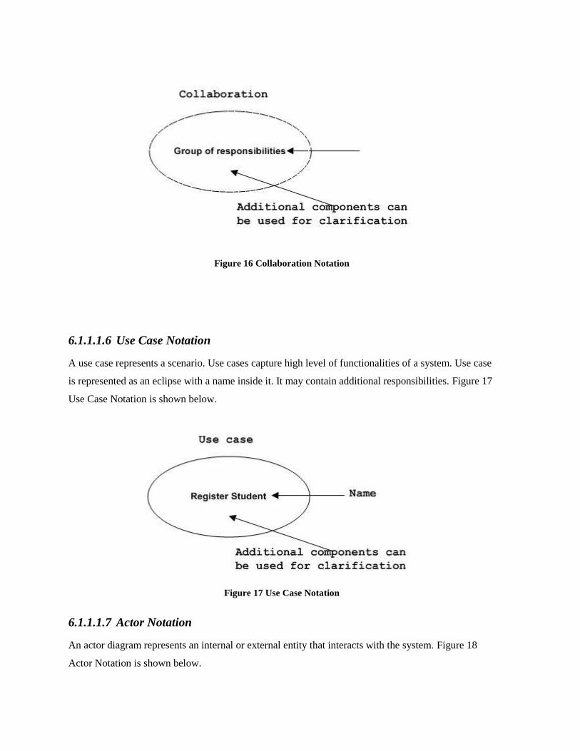
Figure 16 Collaboration Notation

6.1.1.1.6 Use Case Notation

A use case represents a scenario. Use cases capture high level of functionalities of a system. Use case

is represented as an eclipse with a name inside it. It may contain additional responsibilities. Figure 17

Use Case Notation is shown below.

Figure 17 Use Case Notation

6.1.1.1.7 Actor Notation

An actor diagram represents an internal or external entity that interacts with the system. Figure 18

Actor Notation is shown below.

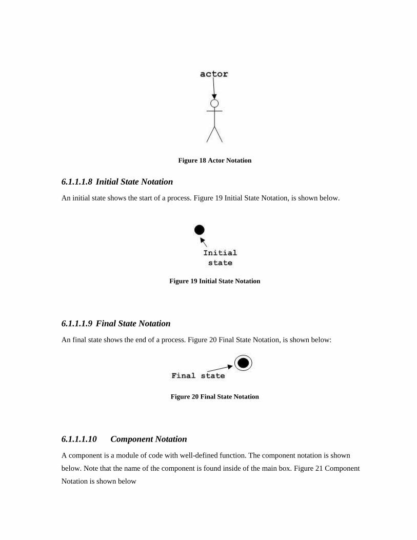
Figure 18 Actor Notation

6.1.1.1.8 Initial State Notation

An initial state shows the start of a process. Figure 19 Initial State Notation, is shown below.

Figure 19 Initial State Notation

6.1.1.1.9 Final State Notation

An final state shows the end of a process. Figure 20 Final State Notation, is shown below:

Figure 20 Final State Notation

6.1.1.1.10 Component Notation

A component is a module of code with well-defined function. The component notation is shown

below. Note that the name of the component is found inside of the main box. Figure 21 Component

Notation is shown below

Figure 21 Component Notation

6.1.1.1.11 Node Notation

A Node in UML represents a physical component of the system like a server or a network. The Figure

22 Node Notation is shown below.

Figure 22 Node Notation

6.1.1.2 Behavioral Elements:

UML’s behavioral elements consist of diagrams that represent dynamic events within the system.

Examples of dynamic events are interactions and state machines.

6.1.1.2.1 Interaction Notation:

Interaction means communication. Interactions are message exchanges between UML components.

Interaction Notations are the sequence diagram and the collaboration diagram. Figure 23 Interaction

Notation is shown below.

Figure 23 Interaction Notation

Figure 24 below presents a sequence diagram and how it makes use of the message notation as the

message flows as calls between the different components of the system in a given scenario.

Figure 24 Interaction Notation in a Sequence Diagram

6.1.1.2.2 State machine notation

The state machine describes the phases of cases that a component goes through in its lifecycle. Figure

25 shows the state notation.

Figure 25 State Notation

Figure 26 shows a sample state-chart diagram. See how the boxes represent changes of state given by

different actions.

Figure 26 State Machine Notation

6.1.1.3 Grouping Elements:

Grouping is an aggregation of elements that jointly serve a common purpose.

6.1.1.3.1 Package Notation

A package wraps components of a system. Figure 27 and Figure 28 show the package notation

Figure 27 Package Notation Explained

Figure 28 Package Notation

6.1.1.4 Annotational Elements:

An annotation refers to notes or comments. UML provides a notation to add comments within

diagrams.

6.1.1.4.1 Note Notation

A note is a comment in a diagram. Figure 29 and Figure 30 present the note notation.

Figure 29 Note Notation Explained

Figure 30 Note Notation

6.1.1.5 Relationships Elements

Relationships between elements refers to the forms of interaction between elements. The types of

relationships in UML follows:

6.1.1.5.1 Dependency Notation

Dependency refers to the need that an element has from another element. Dependency is represented

by a dotted arrow. The arrow head represents the independent element and the other end the

dependent element. Figure 31 presents the dependency notation.

Figure 31 Dependency Notation

6.1.1.5.2 Association Notation

Association describes how many elements take part in an interaction. Association is represented by a

dotted line with or without arrows on both sides. The two ends represent two associated elements as

shown below. The multiplicity is also mentioned at the ends (1, * etc.) to show how many objects are

associated. Association is used to represent the relationship between two elements of a system.

Figure 32 Association Notation is shown below.

Figure 32 Association Notation

6.1.1.5.3 Generalization Notation

Generalization describes the inheritance relationship of the object oriented world. It is parent and

child relationship. Generalization is used to describe parent-child relationship of two elements of a

system. Generalization is represented by an arrow with hollow arrow head as shown below in Figure

33 Generalization Notation Explained. One end represents the parent element and the other end child

element.

Figure 33 Generalization Notation Explained

Figure 34 Generalization Notation

6.1.1.5.4 Realization Notation

It is used to represent interfaces in the OO point of view, in which one component describes some

functionality which is not implemented by the element on the left of the dotted arrow. The element at

the right side of the arrow implements that functionality. Figure 35 presents the realization notation.

Figure 35 Realization Notation

6.1.1.5.5 Extensibility Notation

Additional elements used to represent some extra behavior of the system. These extra behaviors are

not covered by the standard available notations. UML uses the following mechanisms to provide

extensibility features:

Stereotypes (Represents new elements)

Tagged values (Represents new attributes)

Constraints (Represents the boundaries)

Figure 36 presents the extensibility notation.

Figure 36 Extensibility Notation

6.1.2 UML Diagrams

UML identifies two main types of diagrams to describe systems: a) structural diagrams and b)

behavioral diagrams.

6.1.2.1 Structural Modeling Diagrams

Structural Modeling Diagrams help to represent components of the system in a static way. The

structural diagrams are presented in the following sections.

6.1.2.1.1 Class diagram

This is the most common diagram in Object Oriented Architecture. It contains classes, interfaces,

associations and collaborations. Figure 37 shows a sample class diagram.

Figure 37 Class Diagram

6.1.2.1.2 Object Diagram

An object diagram represents a set of objects and their relationships. Figure 38 shows a sample Object

Diagram.

Figure 38 Object Diagram

Scipy.stats Library

Statistical Functions

=====================

This module contains a large number of probability distributions as

well as a growing library of statistical functions.

Each included distribution is an instance of the class rv_continous.

For each given name the following methods are available. See docstring for rv_continuous for more information

:rvs: random variates with the distribution

:pdf: probability density function

:cdf:

cumulative distribution function

:sf:

survival function (1.0 - cdf)

:ppf:

percent-point function (inverse of cdf)

:isf:

inverse survival function

:stats:

mean, variance, and optionally skew and kurtosis

Calling the instance as a function returns a frozen pdf whose shape,

location, and scale parameters are fixed.

REFERENCES

1. GoldSim User’s Guide – Appendix C: Implementing External (DLL) Elements.

(ISO/IEC 19501:2005 Information technology – Open Distributed Processing – Unified Modeling Language

(UML) Version 1.4.2)

2. R. Miles and K. Hamilton, Learning UML 2.0, O’Reilly Media, Inc., 0596009828, 2006.

3. S. C. McConnell, Code Complete, 2nd

ed, Microsoft Press, Redmond, WA, 0735619670, 2004.

UML and SOA Overview with Example Applications to the xLPR ...

Documents

Transcript of UML and SOA Overview with Example Applications to the xLPR ...