ULTRASOUND IMAGE ANALYSIS OF THE CAROTID ARTERY
255
ULTRASOUND IMAGE ANALYSIS OF THE CAROTID ARTERY CHRISTOS P. LOIZOU A THESIS SUBMITTED IN PARTIAL FULLFILMENT OF THE REQUIREMENTS OF THE UNIVERSITY FOR THE DEGREE OF DOCTOR OF PHILOSOPHY (PhD) SCHOOL OF COMPUTING AND INFORMATION SYSTEMS KINGSTON UNIVERSITY LONDON, UK Collaborating Establishments: Intercollege, Cyprus; University of Cyprus; Kingston University, UK; Cyprus Institute of Neurology and Genetics; Academic Vascular Surgery, Imperial College, Faculty of Medicine, Division of Surgery, Anesthetics and Intensive Care, Saint Mary’s Hospital, UK. Submitted: September, 2005
Transcript of ULTRASOUND IMAGE ANALYSIS OF THE CAROTID ARTERY
ULTRASOUND IMAGE ANALYSIS OF
THE CAROTID ARTERY
CHRISTOS P. LOIZOU
A THESIS SUBMITTED IN PARTIAL FULLFILMENT
OF THE REQUIREMENTS OF THE UNIVERSITY FOR
THE DEGREE OF DOCTOR OF PHILOSOPHY (PhD)
SCHOOL OF COMPUTING AND INFORMATION SYSTEMS
KINGSTON UNIVERSITY
LONDON, UK
Collaborating Establishments: Intercollege, Cyprus; University of Cyprus; Kingston University,
UK; Cyprus Institute of Neurology and Genetics; Academic Vascular Surgery, Imperial
College, Faculty of Medicine, Division of Surgery, Anesthetics and Intensive Care, Saint
Mary’s Hospital, UK.
Submitted: September, 2005
Abstract Stroke is one of the most important causes of death in the world and the leading cause of
serious, long-term disability. There is an urgent need for better techniques to diagnose patients
at risk of stroke based on the measurements of the intima media thickness (IMT) and the
segmentation of the atherosclerotic carotid plaque.
The objective of this work was to carry out a comparative evaluation of despeckle filtering
on ultrasound images of the carotid artery, and develop a new segmentation system, for
detecting the IMT of the common carotid artery and the borders of the athrerosclerotic carotid
plaque in longitudinal ultrasound images of the carotid artery. To the best of our knowledge no
similar system has been developed for segmenting the atherosclerotic carotid plaque, although a
number of techniques have been proposed for IMT segmentation.
A total of 11 despeckle filtering methods were evaluated based on texture analysis, image
quality evaluation metrics, and visual evaluation made by two experts, on 440 ultrasound
images of the carotid artery bifurcation. Furthermore, the proposed IMT and plaque
segmentation techniques were evaluated on 100 and 80 longitudinal ultrasound images of the
carotid bifurcation respectively based on receiver operating chatracteristic (ROC) analysis.
The despeckle filtering results showed that a despeckle filter based on local statistics (lsmv)
improved the class separation between asymptomatic and symptomatic classes, gave only a
marginal improvement in the percentage of correct classifications success rate, and improved
the visual assessment carried out by the experts. It was also found that the lsmv despeckle filter
can be used for despeckling asymptomatic images where the expert is interested mainly in the
plaque composition and texture analysis, whereas a geometric despeckle filter (gf4d) can be
used for despeckling of symptomatic images where the expert is interested in identifying the
degree of stenosis and the plaque borders.
The IMT snakes segmentation results showed that no significant difference was found
between the manual and the snakes segmentation measurements. Better segmentation results
were obtained for the normalized despeckled images. The plaque segmentation results showed
that, the Lai&Chin snakes segmentation method gives results comparable to the manual
delineation procedure. The IMT and plaque snakes segmentation method may be therefore used
to complement and assist the final expert’s evaluation.
The proposed despeckling and segmentation methods will be further evaluated on a larger
number of ultrasound images and on multiple experts’ evaluation. Furthermore, it is expected
that both methods will be incorporated into an integrated system enabling the texture analysis of
the segmented plaque, providing an automated system for the early diagnosis and the
assessment of the risk of stroke.
i
Contents Page List of Tables .................................................................................................................vii
List of Figures ................................................................................................................. x
List of Symbols ............................................................................................................xvi
List of Abbreviations ..................................................................................................xxii
Acknowledgements ....................................................................................................xxvi
Chapter 1: Vascular Ultrasound Imaging and Digital Image Processing ................. 1
1.1 Introduction ................................................................................................................2
1.1.1 Risk of stroke.....................................................................................................2
1.1.2 IMT measurements............................................................................................6
1.1.3 Plaque characteristics ........................................................................................7
1.2 A brief review of ultrasound imaging ........................................................................8
1.2.1 Basic principles of ultrasound ........................................................................10
1.2.2 Ultrasound modes ...........................................................................................12
1.2.3 Image quality and resolution ...........................................................................13
1.2.4 Limitations of ultrasound ................................................................................14
1.3 Image processing of the carotid artery .....................................................................15
1.3.1 Despeckle filtering ..........................................................................................16
1.3.2 IMT segmentation ...........................................................................................18
1.3.3 Plaque segmentation........................................................................................19
1.4 Original aspects of the work.....................................................................................20
1.5 Guide to thesis contents............................................................................................22
Chapter 2: Despeckle Filtering .................................................................................... 24
2.1 Introduction ..............................................................................................................25
2.2 Speckle modelling in ultrasound images..................................................................29
2.3 Despeckle filters .......................................................................................................31
2.3.1 Local statistics filters.......................................................................................35
2.3.1.1 First order statistics filtering (lsmv, lsmv_lee, lsmvminmax, lemva,
wiener) .................................................................................................35
2.3.1.2 Local statistics filtering with higher moments (lsmvske1d, lsmvsk2d) ..36
2.3.1.3 Homogeneous mask areas filtering (lsminv, lsminsc, lsminv1d)............37
ii
2.3.1.4 Local statistics 1D filtering (lsmv1d) .....................................................38
2.3.2 Median filtering (median)................................................................................39
2.3.3 Linear scaling filtering (ca, lecasort, ls) .........................................................39
2.3.4 Maximum homogeneity over a pixel neighbourhood filtering (homog) .........39
2.3.5 Geometric filtering (gf4d, gfminmax)..............................................................40
2.3.6 Homomorphic filtering (homo) and logarithmic point operation filtering
(lslog) ..............................................................................................................41
2.3.7 Diffusion filtering............................................................................................42
2.3.7.1 Anisotropic diffusion filtering (ad)........................................................43
2.3.7.2 Lee diffusion and speckle reducing anisotropic diffusion filtering
(lsmedcd, adsr).......................................................................................44
2.3.7.3 Exponential damp kernel filters utilizing diffusion (lsmedc).................45
2.3.7.4 Coherent nonlinear anisotropic diffusion (nldif)....................................46
2.3.8 Wavelet filter (waveltc) ...................................................................................47
Chapter 3: IMT and Plaque Segmentation................................................................. 50
3.1 Introduction .............................................................................................................51
3.2 Previous work on carotid IMT segmentation .........................................................53
3.2.1 On the difference between manual and automated IMT measurements ........56
3.3 Previous work on carotid plaque segmentation .....................................................57
3.4 Active contours (snakes) ........................................................................................60
3.4.1 Approximation of the first order differential ..................................................63
3.4.2 Approximation of the second order differential .............................................63
3.4.3 Approximation of the image energy term .......................................................65
3.4.4 Approximation of the external energy term ....................................................67
3.5 Other snakes approaches ..........................................................................................67
3.5.1 Balloon snake ..................................................................................................68
3.5.2 Lai&Chin snake...............................................................................................69
3.5.3 Gradient vector flow (GVF) snake ..................................................................70
3.6 Snake initialization ...................................................................................................71
3.6.1 IMT contour initialization ...............................................................................72
3.6.2 Plaque contour initialization............................................................................73
Chapter 4: Image Quality, Texture Analysis, and ROC Analysis............................ 74
4.1 Image quality............................................................................................................75
iii
4.2 Optical perception testing procedures ......................................................................77
4.3 Image quality metrics ...............................................................................................78
4.4 Texture analysis .......................................................................................................81
4.4.1 Texture measures.............................................................................................82
4.4.2 Feature selection..............................................................................................83
4.4.3 kNN Classifier .................................................................................................83
4.5 ROC analysis ...........................................................................................................84
4.5.1 Performance metrics for detection problems...................................................84
4.5.2 Evaluation of the plaque segmentation ...........................................................87
Chapter 5: Methodology .............................................................................................. 89
5.1 Material ....................................................................................................................90
5.2 Acquisition ...............................................................................................................91
5.3 Image normalisation .................................................................................................92
5.4 Generation of an artificial carotid image..................................................................94
5.5 Image quality of two ultrasound scanners ................................................................94
5.6 Despeckle filtering ...................................................................................................94
5.6.1 Visual perception evaluation ...........................................................................95
5.6.2 Texture analysis...............................................................................................97
5.6.3 Image quality evaluation metrics.....................................................................97
5.7 IMT segmentation ..................................................................................................98
5.7.1 Manual measurements and visual perception evaluation ................................98
5.7.2 IMT initialisation .........................................................................................100
5.7.3 IMT segmentation .........................................................................................102
5.7.4 Univariate statistical analysis ........................................................................105
5.7.5 Correlation analysis .......................................................................................107
5.8 Plaque segmentation...............................................................................................107
5.8.1 Manual measurements and visual perception evaluation ..............................107
5.8.2 Plaque initialisation using the blood flow image...........................................111
5.8.3 Plaque segmentation......................................................................................113
5.8.4 ROC analysis of plaque segmentation methods ............................................114
Chapter 6: Results....................................................................................................... 116
6.1 Image quality evaluation of two ultrasound scanners ............................................117
6.1.1 Visual perception...........................................................................................117
iv
6.1.2 Statistical and texture features.......................................................................120
6.1.3 Quality evaluation metrics.............................................................................122
6.2 Despeckle filtering .................................................................................................124
6.2.1 Despeckle filtering on an artificial and a real carotid image .........................124
6.2.2 Texture analysis.............................................................................................129
6.2.3 Image quality evaluation metrics...................................................................133
6.2.4 Visual perception by experts .........................................................................134
6.2.5 Additional comments by experts ...................................................................135
6.3 IMT segmentation ..................................................................................................138
6.3.1 An example of IMT segmentation.................................................................138
6.3.2 Univariate statistical analysis ........................................................................140
6.3.3 Regression and correlation analysis ............................................................148
6.4 Plaque segmentation...............................................................................................155
6.4.1 Examples of plaque segmentation .................................................................155
6.4.2 Evaluation of plaque segmentation methods ................................................161
Chapter 7: Discussion ................................................................................................. 165
7.1 Image quality evaluation of two ultrasound scanners ............................................166
7.1.1 Visual perception...........................................................................................166
7.1.2 Statistical and texture measures.....................................................................166
7.1.3 Quality evaluation metrics.............................................................................167
7.1.4 Summary findings on image quality evaluation ............................................167
7.2 Despeckle filtering .................................................................................................168
7.2.1 Despeckle filtering on an artificial and a real carotid image .........................169
7.2.2 Texture analysis.............................................................................................171
7.2.3 Image quality evaluation metrics...................................................................172
7.2.4 Visual perception and additional comments by experts ................................174
7.2.5 Summary findings on despeckle filtering .....................................................175
7.3 IMT segmentation .................................................................................................179
7.3.1 IMT snakes segmentation .............................................................................179
7.3.2 Univariate statistical analysis ........................................................................182
7.3.3 Regression and correlation analysis ..............................................................187
7.3.4 Summary findings on IMT segmentation .....................................................189
7.4 Plaque segmentation...............................................................................................190
7.4.1 Plaque snakes segmentation ..........................................................................190
7.4.2 Evaluation of plaque segmentation methods .................................................193
v

7.4.3 Summary findings on plaque segmentation .................................................195
7.5 Proposed system.....................................................................................................196
Chapter 8: Conclusions and Future Work ............................................................... 198
8.1 Conclusions ............................................................................................................199
8.2 Future work ..........................................................................................................201
Appendix I: Statistics of Speckle ............................................................................... 204
Appendix II: Optical Perception Testing Procedure Evaluations ......................... 208
Appendix III: Texture Measures .............................................................................. 212
Appendix IV: Complete Snake Implementation ..................................................... 224
Appendix V: List of Publications............................................................................... 230
References .................................................................................................................... 307
vi

LIST OF TABLES
List of Tables PAGE
TABLE 2.1 AN OVERVIEW OF DESPECKLE FILTERING TECHNIQUES 33
TABLE 3.1 AN OVERVIEW OF ULTRASOUND SEGMENTATION TECHNIQUES IN
VASCULAR IMAGING
53
TABLE 3.2 AN OVERVIEW OF PLAQUE SEGMENTATION TECHNIQUES IN VASCULAR
IMAGING
58
TABLE 6.1 VISUAL PERCEPTION EVALUATION FOR THE IMAGE QUALITY ON 80
IMAGES PROCESSED FROM EACH SCANNER FOR THE ORIGINAL (NF),
DESPECKLED (DS), NORMALIZED (N), AND NORMALIZED DESPECKLED
(NDS). SCORES ARE EXPRESSED IN PERCENTAGE FORMAT
120
TABLE 6.2 STATISTICAL AND TEXTURE FEATURES (MEAN VALUES FOR 80 IMAGES
PROCESSED FROM EACH SCANNER) FOR THE ORIGINAL (NF),
DESPECKLED (DS), NORMALIZED (N) AND NORMALIZED DESPECKLED
(NDS) IMAGES
121
TABLE 6.3 IMAGE QUALITY EVALUATION METRICS BETWEEN THE ORIGINAL-
DESPECKLED (NF-DS), THE ORIGINAL-NORMALIZED (NF-N), THE
ORIGINAL-NORMALIZED DESPECKLED (NF-NDS) AND THE
NORMALIZED-NORMALIZED DESPECKLED (N-NDS) IMAGES
122
TABLE 6.4 SELECTED STATISTICAL FEATURES FOR FIG. 6.3A BEFORE AND AFTER
DESPECKLE FILTERING. BOLDED VALUES SHOW IMPROVEMENT AFTER
DESPECKLE FILTERING
127
TABLE 6.5 FEATURE DISTANCE (4.13) AND SCORE_DIS (4.14) FOR SF, SGLDM
RANGE OF VALUES, AND NGTDM TEXTURE FEATURES SETS BETWEEN
ASYMPTOMATIC AND SYMPTOMATIC CAROTID PLAQUE ULTRASOUND
IMAGES. BOLDED VALUES SHOW IMPROVEMENT AFTER DESPECKLE
FILTERING
130
TABLE 6.6 WILCOXON RANK SUM TEST FOR THE SGLDM RANGE OF VALUES
TEXTURE FEATURES APPLIED ON THE 440 ULTRASOUND IMAGES OF
CAROTID PLAQUE BEFORE AND AFTER DESPECKLE FILTERING. THE
TEST SHOWS WITH S SIGNIFICANT DIFFERENCE AFTER FILTERING AT
P<0.05 AND NS NO SIGNIFICANT DIFFERENCE AFTER FILTERING AT
P>=0.05. THE P VALUE IS ALSO GIVEN IN PARENTHESIS
131
vii

LIST OF TABLES
TABLE 6.7 PERCENTAGE OF CORRECT CLASSIFICATIONS SCORE FOR THE KNN
CLASSIFIER WITH K=7 FOR THE ORIGINAL AND THE DESPECKLED IMAGE
SETS. BOLDED VALUES INDICATE IMPROVEMENT AFTER DESPECKLING
132
TABLE 6.8 IMAGE QUALITY EVALUATION METRICS COMPUTED FOR THE 220
ASYMPTOMATIC AND 220 SYMPTOMATIC IMAGES
133
TABLE 6.9.1 PERCENTAGE SCORING OF VISUAL EVALUATION OF THE ORIGINAL AND
DESPECKLED IMAGES (50 ASYMPTOMATIC (A) AND 50 SYMPTOMATIC
(S)) BY THE EXPERTS
134
TABLE 6.9.2 PERCENTAGE SCORING OF VISUAL EVALUATION OF THE ORIGINAL AND
DESPECKLED IMAGES (50 ASYMPTOMATIC (A) AND 50 SYMPTOMATIC
(S)) BY THE EXPERTS ONE YEAR AFTER THE FIRST VISUAL EVALUATION
135
TABLE 6.10 ADDITIONAL COMMENTS ON DESPECKLE FILTERING MADE BY THE
EXPERTS
137
TABLE 6.11 COMPARISON BETWEEN THE MANUAL AND THE SNAKES SEGMENTATION
MEASUREMENTS FOR THE CASES B-H IN FIGURE 6.6. MEASUREMENTS
ARE IN MILLIMETERS (MM)
138
TABLE 6.12.1 COMPARISON BETWEEN MANUAL AND SNAKES SEGMENTATION
MEASUREMENTS FOR THE 100 ULTRASOUND IMAGES OF THE CAROTID
ARTERY. MEASUREMENTS ARE IN MILLIMETRES (MM). BOLDED VALUES
SHOW BEST PERFORMANCE
141
TABLE 6.12.2 IMT MANUAL MEASUREMENTS (IN MM) FOR THE 100 ULTRASOUND
IMAGES OF THE CAROTID ARTERY PERFORMED BY THE TWO VASCULAR
EXPERTS
141
TABLE 6.12.3 WILCOXON RANKSUM TEST FOR THE IMT MANUAL SEGMENTATION
MEASUREMENTS. THE TEST SHOWS WITH S SIGNIFICANT DIFFERENCE
AFTER FILTERING AT P<0.05 AND NS NO SIGNIFICANT DIFFERENCE
AFTER FILTERING AT P>=0.05. THE P VALUES ARE ALSO SHOWN IN
PARENTHESIS.
142
TABLE 6.13.1 TESTS AND MEASURES COMPUTED ON 100 ULTRASOUND IMAGES OF
THE CAROTID ARTERY FROM THE FIRST EXPERT. LEFT COLUMN UPPER
TRIANGLE: WILCOXON RANK SUM TEST (S=SIGNIFICANTLY DIFFERENT
AFTER FILTERING AT P<0.05, NS=NOT SIGNIFICANTLY DIFFERENT
AFTER FILTERING AT P>=0.05). THE P VALUES ARE ALSO SHOWN IN
PARENTHESIS. LEFT COLUMN LOWER TRIANGLE: VARIATION OF THE
144
viii
LIST OF TABLES
HAUSDORFF DISTANCE (*10-3). RIGHT COLUMN UPPER TRIANGLE:
COVARIANCE, . RIGHT COLUMN LOWER TRIANGLE: MEAN-SQUARE
ERROR (*10-3). BOLDED VALUES SHOW BEST PERFORMANCE. THE LEVEL
OF SIGNIFICANCE IS ALSO SHOWN IN BRACKETS.
amc ,
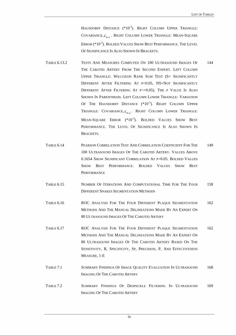
TABLE 6.13.2 TESTS AND MEASURES COMPUTED ON 100 ULTRASOUND IMAGES OF
THE CAROTID ARTERY FROM THE SECOND EXPERT. LEFT COLUMN
UPPER TRIANGLE: WILCOXON RANK SUM TEST (S= SIGNIFICANTLY
DIFFERENT AFTER FILTERING AT P<0.05, NS=NOT SIGNIFICANTLY
DIFFERENT AFTER FILTERING AT P>=0.05). THE P VALUE IS ALSO
SHOWN IN PARENTHESIS. LEFT COLUMN LOWER TRIANGLE: VARIATION
OF THE HAUSDORFF DISTANCE (*10-3). RIGHT COLUMN UPPER
TRIANGLE: COVARIANCE, . RIGHT COLUMN LOWER TRIANGLE:
MEAN-SQUARE ERROR (*10-3). BOLDED VALUES SHOW BEST
PERFORMANCE. THE LEVEL OF SIGNIFICANCE IS ALSO SHOWN IN
BRACKETS.
amc ,
144
TABLE 6.14 PEARSON CORRELATION TEST AND CORRELATION COEFFICIENT FOR THE
100 ULTRASOUND IMAGES OF THE CAROTID ARTERY. VALUES ABOVE
0.1654 SHOW SIGNIFICANT CORRELATION AT P<0.05. BOLDED VALUES
SHOW BEST PERFORMANCE. BOLDED VALUES SHOW BEST
PERFORMANCE
149
TABLE 6.15 NUMBER OF ITERATIONS AND COMPUTATIONAL TIME FOR THE FOUR
DIFFERENT SNAKES SEGMENTATION METHODS
158
TABLE 6.16 ROC ANALYSIS FOR THE FOUR DIFFERENT PLAQUE SEGMENTATION
METHODS AND THE MANUAL DELINEATIONS MADE BY AN EXPERT ON
80 ULTRASOUND IMAGES OF THE CAROTID ARTERY
162
TABLE 6.17 ROC ANALYSIS FOR THE FOUR DIFFERENT PLAQUE SEGMENTATION
METHODS AND THE MANUAL DELINEATIONS MADE BY AN EXPERT ON
80 ULTRASOUND IMAGES OF THE CAROTID ARTERY BASED ON THE
SENSITIVITY, R, SPECIFICITY, SP, PRECISION, P, AND EFFECTIVENESS
MEASURE, 1-E
162
TABLE 7.1 SUMMARY FINDINGS OF IMAGE QUALITY EVALUATION IN ULTRASOUND
IMAGING OF THE CAROTID ARTERY
168
TABLE 7.2 SUMMARY FINDINGS OF DESPECKLE FILTERING IN ULTRASOUND
IMAGING OF THE CAROTID ARTERY
169
ix

LIST OF FIGURES
List of Figures PAGE
Fig. 1.1 World leading causes of death (US CDC National center of health
statistics, vital statistics of the United States, Annual 2000).
3
Fig. 1.2 (a) The carotid system [130], (b) longitudinal section of a carotid
artery with plaque (left) and embolisation (right) [153] (c) transverse
section of a carotid artery with plaque, (e) stable and unstable plaque.
(From Heart Center online: http://www.heartcenteronline.com).
4
Fig. 1.3 Ultrasound imaging scanners: (a) ATL HDI-3000, (b) ATL HDI-5000
[153].
9
Fig. 1.4 Longitudinal color flow duplex image of the carotid artery combined
with Doppler ultrasound image. Highlighted image with white contour
on top shows the carotid bifurcation. The 2D signal shows the
velocity variation related to the cardiac cycle. Blood flow velocity
spectrum is displayed with markings 1 and 2, where marking 1
represents the peak systolic velocity and marking 2 represents the end
diastolic velocity. This is the duration of one cardiac cycle. Different
colours represent blood flow direction. For the current picture, red
represents the blood moving to the brain through the carotid artery,
whereas blue represents the blood returning back from the brain.
11
Fig. 1.5 Ultrasound B-mode longitudinal image of the carotid bifurcation with
manually outlined plaque, which is usually confirmed with blood flow
image.
13
Fig. 1.6 Close view of manual measurement of the IMT: (1) 0.9 mm, (2) 0.8
mm, (3) 0.86 mm.
16
Fig. 1.7 Results of despeckle filtering based on first order local statistics.
Asymptomatic case: (a) original, (c) despeckled, (e) enlarged region
marked in c) of the original, (g) enlarged region marked in c) of the
despeckled image. Symptomatic case: (b) original, (d) despeckled, (f)
enlarged region marked in d) of the original, (h) enlarged region
marked in d) of the despeckled image. Regions were enlarged by a
factor of three.
17
x
LIST OF FIGURES
Fig. 1.8 Ultrasound image of the carotid artery for an asymptomatic case: (a)
detected initial contours for the IMT, and (b) final contours after
snakes deformation. = 0.86 mm, = 1.04 mm,
= 0.73 mm, = 0.83 mm.
meanIMT maxIMT
minIMT medianIMT
18
Fig. 1.9 Ultrasound image of the carotid artery: (a) plaque initial contour
estimation, and (b) the final plaque contour after the snakes
deformation.
20
Fig. 2.1 The usual tissue model in ultrasound imaging, modified from [199]. 26
Fig. 2.2 (a) The scattering in the sound beam, (b) one pulse (from [14]). 27
Fig. 2.3 The processing steps of the RF-signal inside the ultrasound scanner,
modified from [156].
28
Fig. 2.4 Schematical operation of the filters: (a) lsmv and (b) lsminv1d
respectively.
38
Fig. 2.5 (a) Directions of implementation of the gf4d geometric filter, (b)
pixels selected for the NS direction (intensity of central pixel b is
adjusted based on the values of intensities of pixels a, b, and c).
41
Fig. 3.1 (a) Illustration of the intima-media (IM). IM contains the area between
the intima and adventitia. The sub-intima region may cause problems
in searching the adventitia layer due to speckle noise and due to its
interference caused from the adventitia layer. (b) Intensity schematic
illustration of a lumen-intima and media-adventitia interface at the far
wall of the carotid artery. Modified from [253].
57
Fig: 3.2 Illustration of the snake contour deformation. Open circles represent
snake points that are candidates to replace the original (solid) point.
62
Fig. 4.1 DSCQS method: (a) the reference and the test sequence are presented
twice in alternated fashion, (b) the order of the two is chosen
randomly for each trial, and experts are not informed which is which.
They rate each of the two separately on a continuous quality scale
ranging from bad to excellent (Modified from [7] pp. 572, Fig. 10.1).
78
Fig. 4.2 Definition of TP, FN, FP, and TN. 85
xi
LIST OF FIGURES
Fig. 4.3 (a) Intersection, and (b) union of two variables, and GT. AS 88
Fig. 5.1 Normalization of a carotid ultrasound image: two reference points are
selected in order to normalize the image: (a) blood area is selected
and, (b) adventitia area located over the plaque is selected.
93
Fig. 5.2 The graphical user interface for the visual image evaluation carried
out by the experts. The screen illustrates four different despeckled
images and their corresponding scores.
96
Fig. 5.3 Demonstration of the manual IMT segmentation module. 99
Fig. 5.4 IMT contour initialization procedure and final snakes contours: (a)
Original ultrasound image with selected area, (b) cropped area, (c)
despeckled area, (d) binary cropped area, (e) dilated cropped area, (f)
dilated area after removal of small edges, (g) construction of the
interpolating B-spline, (h) detected initial contours for the adventitia
and the intima layers, and (i) final contours after the snake
deformation. The , is shown with double line box, the
, with a full line box and the , with dashed line box.
meanIMT
maxIMT minIMT
101
Fig. 5.5 Edge map of an artificial carotid image of the original image in Fig.
6.3a, and the detected initial contours for the IMT.
103
Fig. 5.6 Demonstration of the IMT segmentation module. 104
Fig. 5.7 Types of plaque: (a) blood flow image for the type I plaque, (b) type I
plaque: the plaque is not visible, (c) type II plaque: bright echoes
occupy < 50% of plaque, (d) type III: bright echoes occupy 50%-80%
of plaque, (e) type IV: bright echoes occupy 80%-100% of plaque, (f)
type V plaque: calcified plaque where borders cannot be visualized
well.
109
Fig. 5.8 Selection of a plaque: (a) The gray scale image and the blood flow
colour image are loaded, (b) expert has selected a log transform on the
gray scale image for better visualising the plaque, and (c) the final
selected plaque is saved.
110
Fig. 5.9 Plaque initialization using the blood flow image procedure: (a)
O i i l l d B d i f id i h l
112
xii
LIST OF FIGURES
Original ultrasound B-mode image of a carotid artery with plaque at
the far wall, (b) blood flow image, (c) initial blood flow edge contour
with the area for the initial contour selected by the expert, (d) sampled
initial snake contour, (e) snakes segmentation of plaque, and (f)
manual segmentation of plaque.
Fig. 5.10 Demonstration of the plaque segmentation module. 113
Fig. 6.1 Ultrasound carotid artery images, taken from one patient at the Cyprus
Institute of Neurology and Genetics, of the original (NF), despeckled
(DS), normalized (N), and normalized despeckled (NDS) of the ATL
HDI-3000, and ATL HDI-5000 shown in the left and right columns
respectively.
118
Fig. 6.2 Line profiles for the NF, DS, N, and NDS images, for the ATL HDI-
3000, and ATL HDI-5000 scanner, shown in the left and right
columns respectively. The gray scale values, and the column 240, are
shown in the y- and x-axis.
119
Fig. 6.3 Original noisy image of an artificial carotid artery given in (a), and the
application of the 11 despeckle filters given in (b)-(l). (Vertical line
given in (a) defines the position of the line intensity profiles plotted in
Fig. 6.4).
125
Fig. 6.4 Line profiles of the line illustrated in Fig. 6.3a for the original noisy
image (a), and the 11 despeckled images given in (b)-(l).
126
Fig. 6.5 Original ultrasound image of the carotid artery (2-3 cm proximal to
bifurcation) given in (a), and the despeckled images given in (b)-(l).
128
Fig. 6.6 (a) Original longitudinal ultrasound image of the carotid artery, (b)
manual delineation from the first expert, (c) manual delineation from
the second expert, (d) initial contour estimation, and the segmentation
results of the IMT for (e) no filtering (NF), (f) despeckled (DS), (g)
normalized (N), and (h) normalized despeckled (NDS) images. The
detected , , and are shown with a double,
single, and dashed line boxes respectively.
meanIMT maxIMT minIMT
139
Fig. 6.7 Increase of with: (a) age and (b) systolic blood pressure. meanIMT 142
xiii
LIST OF FIGURES
Fig. 6.8 Histograms of the values for the: (a) manual first set of
measurements from first expert (M1F), (b) manual normalized first set
of measurements from first expert (MN1F), (c) manual first set of
measurements from second expert (M2F), (d) manual normalised first
set of measurements from second expert (MN2F), (e) no filtering
(NF), (f) despeckle (DS), (g) normalised (N), and (h) normalized
despeckled (NDS), images.
meanIMT 146
Fig. 6.9 Box plots for the values in mm: (a) for the manual and manual
normalized first set of measurements, from expert one (M1F, MN1F)
and expert two (M2F, MN2F), and (b) for the Williams&Shah snakes
segmentation cases NF, DS, N, and NDS respectively.
meanIMT 147
Fig. 6.10 A scatter plot with least squares regression line for the inter-observer
variability of the manual IMT delineation between the two experts for
100 ultrasound images of the carotid artery, on: (a) the original (M),
and (b) the normalised (MN) images.
148
Fig. 6.11 Comparison of manually and snakes segmented IMT borders with
regression lines, showing the correlations between: (a) the NF-M1F,
(b) NF-MN1F, (c) DS-MN1F, (d) N-MN1F, (e) NDS-MN1F, (f) DS-
M1F, (g) N-M1F, and (h) NDS-M1F detected IMT boundaries.
150
Fig. 6.12 Regression lines (Bland-Altman plots) of manual versus
Williams&Shah snakes segmentation method for the IMTmean for the
first set of measurements for both experts. The middle line represents
the mean difference, and the upper and lower two outside lines
represent the limits of agreement between the two methods, which are
the mean of the data sd2± for the estimated difference between the
two methods.
154
Fig. 6.13 Segmentation results on a longitudinal ultrasound B-mode image of
the carotid artery with plaque, with: (a) manual segmentation, (b)
Williams&Shah, (c) Balloon, (d), Lai&Chin, (e) GVF snake, and (f)
segmentation contours computed in (b)-(e) superimposed.
156
Fig. 6.14 Segmentation results on a longitudinal ultrasound B-mode image of
the carotid artery with plaque, with: (a) manual segmentation, (b)
Williams&Shah, (c) Balloon, (d), Lai&Chin, (e) GVF snake, and (f)
157
xiv
LIST OF FIGURES
all segmentation contours computed in (b)-(e) superimposed.
Fig. 6.15 Segmentation results on a longitudinal ultrasound B-mode image of
the carotid artery with plaque at the near wall, with: (a) manual
segmentation, and (b) Williams&Shah (red line), Balloon (blue line),
Lai&Chin (yellow line), and GVF (green line), snakes segmentation
contours computed superimposed.
158
Fig. 6.16 Plots of the total snake energy for: (a) the Williams&Shah (TSEP), (b)
Balloon (TSEB), (c) Lai&Chin (TSELC), and (d) GVF snake
(TSEGVF) for the image in Fig. 6.14a.
159
Fig. 6.17 Plots of the snake energy terms versus the number of iterations for the
Williams&Shah snakes segmentation method for the image in Fig.
6.14, for: (a) normalized total snake energy (NTSE), (b) normalized
continuity energy (NCE), (c) normalized curvature energy (NCRE),
and (d) normalized image energy (NIE) terms respectively.
160
Fig. 6.18 Plots for the α and β snake parameters for the Lai&Chin snakes
segmentation method versus the number of iterations.
161
Fig. 6.19 Box plots for the four snakes segmentation methods (Williams&Shah,
Balloon, Lai&Chin, and GVF) for: (a) TPF, (b) TNF, (c) FPF, (d)
FNF, (e) Williams index, KI and (f) overlap index.
163
Fig. 6.20 ROC curve analysis based on the TPF and FPF fractions for the four
snakes segmentation methods.
164
xv

LIST OF SYMBOLS
List of Symbols
A Pentavector (matrix)
maxA , minA Maximum and minimum values of the signal A
iA Average gray-tone over a neighbourhood
A Input ultrasound signal to the amplifier
)(sα Snake tension parameter of the energy functional
GVFα GVF snake elasticity parameter
jia , Additive noise component on pixel ji,
visualα Degrees of visual angle
a A non-zero parameter
compcomp βα , Logarithmic compression parameters
)(sβ Snake stiffness of the energy functional
GVFβ GVF snake rigidity parameter
C Speckle Index
%CV Coefficient of variation
amCov , Covariance between automated and manual measurements
am
amam
Covc
σσ,
, = Correlation, for the strength of the relationship between
automated and manual methods
)( gcd ∇ , jic , Diffusion coefficient
adsrc Speckle reducing anisotropic diffusion coefficient
c Constant controlling the magnitude of the potential
2sin_1sin_ , ss cc Constants used to calculate the SSIN
2c Positive weighting factor
Γ Number of directions, which diffusion is computed
)(sγ Influence of image gradients on energy snake functional
γ Signal-to-noise radio (SNR)
2
2 )(ds
sdv Second order snake differential
dssdv )(
First order snake differential
22 xD ℜ∈ Symmetric positive semi-definite diffusion tensor representing
xvi

LIST OF SYMBOLS
the required diffusion in both gradient and contour directions
Df Fractal dimension
D Matrix used to calculated the image energy of the snake,
)(vEimage
viewingD Viewing distance
DR Dynamic range of input ultrasound signal
)(kd Wavelet coefficient for the wavelet filtering
min,ICAd Minimum lumen diameter in the ICA
distalICAd , Lumen diameter in a distal diseased free portion of the ICA
cidis , Distance between asymptomatic and symptomatic images
d Average distance between snake vertices
∆ Snake convergence scalar factor
)(sδ Snake contour damping density
),( yx ∆∆≡δ Displacement of a pixel at direction (x, y)
f∆ Frequency shift (Doppler frequency shift)
r∆ Distance between two pixels
g∇ The gradient magnitude of image (gradient) ),( yxg
jig ,∇ Directional derivative (simple difference) at location ji,
ming∇ , maxg∇Maximum and minimum gradient values in a pixel
neighbourhood
g∆ Intensity difference between two pixels
{}E Expectation operation
}{XE Expected value of the reflected ultrasound signal X
)(vEsnake Snake energy function
)(int vE Snake internal energy
)(vEcont Snake continuity energy
)(vEcurv Snake curvature energy
)(vEimage Snake image energy
)(vEexternal External snake energy
)(vEline Line energy of the snake
)(vEedge Edge energy of the snake
ε Constant for the snake points length adjustment in )(int vE
xvii
LIST OF SYMBOLS
normalF Normal force, added to the energy snake functional
131... ff SGLDM texture measures from Haralick
),( yxf x First order differential of the edge magnitude along the x-axis
vF Vertical force, added to the snake energy functional
jif , Noise-free signal ultrasound signal in discrete form (the new
image) on pixel ji,
f Frequency of ultrasound wave
0f Transmitted frequency of ultrasound signal
spatfmax_ Maximum spatial frequency
idisfeat _ Percentage distance
jig , Observed ultrasound signal in discrete formulation after
logarithmic compression
),( yxg Observed ultrasound signal after logarithmic compression,
representing image intensity at location (x, y)
G Linear gain of the amplifier
jigG ,*σ Image convolved with Gaussian smoothing filter
σG Gaussian smoothing filter
ig , if Mean gravity of the searching pixel region in image g or f
maxg , mingMaximum and minimum gray level values in a pixel
neighbourhood
Hz , KHz , MHz Hertz, Kilohertz, Megahertz
HX, HY Entropies of px and py )(kH Hurst coefficients
),( yxH Array of points of the same size for the HT
screenH Screen height
)(AH Frequency response of the pentavector A
HD Hausdorff distance
h Distance between two consecutive snake points and 1, −jiv jiv ,
sη Spatial neighborhood of pixel ji,
sη Number of neighbors (usually four except at the image
boundaries)
iθ Phase shift relative to the insonated ultrasound wave
xviii

LIST OF SYMBOLS
θ Angle between the direction of movement of the moving object
and the ultrasound beam
I Identity matrix
)(0 xI Modified Bessel function of the first kind of order 0
71 II − Echo boundaries describing the regions in carotid artery
meanIMT Mean value of the IMT
minIMT IMT minimum value
maxIMT IMT maximum value
medianIMT IMT median value
)(kid Average of the absolute intensity difference.
(.)ζK Modified Bessel function of the second kind of order ζ
(.)αK Modified Bessel function of the second kind of order α
K Damping factor
k Coefficient of variation for speckle filtering
L Snake contour length
scanL Number of scan lines for a display (screen)
jilpg , Low passed filtered of the original image at location ji,
λ Wavelength of ultrasound wave
πλ Lai&Chin snake energy regularisation parameter, )(vEsnake
+ℜ∈dλ Rate of diffusion for the anisotropic diffusion filter
errorrelativemean __ Mean relative error
1im , 2im Mean values of two classes (asymptomatic, symptomatic)
sm / , scm / Metres per second, centimetres per second µ Mean
)(sµ Snake contour mass density
GVFµ GVF snake regularisation parameter
N Number of scatterers within a resolution cell
featN Number of features in the feature set
gN Number of distinct gray levels in the quantized image
jin , Multiplicative noise component (independent of , with mean 0) on pixel
jig ,
ji,
jinl , Multiplicative noise component after logarithmic compression
i l ji
xix

LIST OF SYMBOLS
on pixel ji, )(sn Normal force tensor
iξ Amount of ultrasound signal backscattered by scatterer i
),( irXX XXpir
Joint intensity distribution (density function) of the real and the imaginary part of the ultrasound signal X
)(XpX Probability distribution of X
))(( svP Snake scalar potential function
),( jip thji ),( entry in the normalised SGLDM
)(xpr Rice distribution with variance ασ /2 x
)(xpγ Gamma distribution
)(ipx ith entry in the marginal probability matrix obtained by
summing the rows of ),( jip
Q Mathematically defined universal quality index
2111σ+
−=R Smoothness of an image
pearsonr Pearson product moment correlation coefficient
corelρ Correlation coefficient
ρ Normal force, weighting factor normalF
DisScore _ Score distance between two classes (asymptomatic,
symptomatic)
2/IMTes σ= Inter-observer error
maxs Maximum pixel value in the image
2s Structural energy
IMTσ IMT standard deviation
fgσ Covariance between two images and f g
σ Standard deviation 2σ Variance
3σ Skewness
4σ : Kurtosis
1iσ , 2iσ Standard deviations of two classes (asymptomatic, symptomatic)
22σ Diffuse energy
nσ Standard deviation of the noise
xx

LIST OF SYMBOLS
s Arc length of the snake contour
τ Time constant, controls the next iteration of the snake
spu Speed of sound through tissue
1, −jiv , , jiv , 1, +jiv Precedent, current and next snake contour points
ν Velocity of ultrasound wave propagation
),( tsv Element along the snake contour, )](),([)( sysxsv =
iancewindow var_ Variance of the gray values in a pixel window
X Reflected ultrasound signal
maxX , minX Maximum and minimum values of the signal X
jix , Noise free signal before logarithmic compression in discrete
form on pixel ji,
,rX iX Real and imaginary part of the reflected ultrasound signal X
X Amplitude of the reflected ultrasound signal
2),( ℜ∈yx Spatial coordinates of an image
jiz , Original ultrasound signal before logarithmic compression in
discrete form on pixel ji,
71 ZZ − Echo zones describing the regions in carotid artery
lineω Sign of the line energy functional
edgeω Sign of the edge energy functional
I Intersection between two areas
U Union between two areas
# Number of elements in a set
xxi
LIST OF ABBREVIATIONS
List of Abbreviations
ACSRS Asymptomatic Carotid Stenosis
ad Perona and Malik anisotropic diffusion filter
adsr Speckle reducing anisotropic diffusion filter
AS Automatic segmented area
ASM Angular second moment
ATL HDI-3000 ATL 3000 ultrasound scanner
ATL HDI-5000 ATL 5000 ultrasound scanner
ca Linear scaling of the gray-levels despeckle filter
CAT Computer assisted tomography
CCA Common carotid artery
CSR Contrast-to-speckle radio
CT Computer tomography
CW Continuous wave
DR Dynamic range
DS Despeckled
DSCQS Double stimulus continuous quality scale
DSIS Double stimulus impairment scale
DVD Digital video
DWT Discrete wavelet transform
E Effectiveness measure
ECA External carotid artery
ECST European carotid surgery trial
EROS Evaluation of risk of stroke
Err Error summation in the form of the Minkowski metric
fdf Frequency domain despeckle filter
FDTA Fractal dimension texture analysis
FFT Fast Fourier transform
FN False negative
FNF False negative fraction
FP False positive
FPF False positive fraction
FPS Fourier power spectrum
GA Genetic algorithms
GACs Geometric active contours
GAE Geometric average error
xxii
LIST OF ABBREVIATIONS
GF Geometric filtering
gf4d Geometric despeckle filter
gfminmax Geometric despeckle filter utilising minimum maximum values
GGVF Generalised gradient vector flow
GHT Generalised Hough transform
GLDS Gray level difference statistics
GT Segmented area representing ground truth
GVF Gradient vector flow
HD Hausdorff distance
HDI Lab QLAB quantification software
HF Maximum homogeneity
HM Homomorphic
homo Homomorphic despeckle filter
homog Most homogeneous neighbourhood despeckle filter
HT Hough transform
HVS Human visual system
ICA Internal carotid artery
ICRU International commission of radiation units and measurements
IDM Inverse difference moment
IDV Intensity difference vector
IMC Intima media complex
IMT Intima media thickness
IVUS Intra Vascular ultrasound
KI Similarity kappa index
kNN The statistical k-nearest-neighbour classifier
lecasort Linear scaling and sorting despeckle filter
lemva Mean and variance local statistics despeckle filter
LS Linear scaling
ls Linear scaling of the gray level values despeckle filter
lslog Linear scaling of gray values logarithmic despeckle filter
lsmedc Diffusion exponential damp kernel despeckle filter
lsmedcd Lee diffusion despeckle filter
lsminsc Minimum speckle index homogeneous mask despeckle filter
lsminv1d Minimum variance homogeneous 1D mask despeckle filter
lsmv Mean and variance local statistics despeckle filter
lsmv_lee Lee local statistics despeckle filter
lsmvsk2d Mean variance, higher moments local statistics despeckle filter
xxiii
LIST OF ABBREVIATIONS
lsmvske1d Mean, variance, skewness, kurtosis 1D local statistics despeckle
filter
M Manual
median Median despeckle filter
MF Multi-resolution fractal
MMSE Minimum mean-square error
MN Manual normalised
MRI Magnetic resonance imaging
MSE Mean square error
N Normalized
NASCET North American symptomatic carotid endarterectomy trial
NCE Normalised continuity energy
NCRE Normalised curvature energy
ND Normalized despeckled
NE North east
NF No filtering
NGTDM Neighbourhood gray tone difference matrix
NIE Normalised image energy
nldif Non-linear coherent diffusion despeckle filter
NS Not significant difference
NST North south
NTSE Normalised total snake energy
Overlap Overlap value of two areas
P Precision
PACs Parametric active contours
PDE Partial differential equation
PDF Probability density function
PET Positron emission tomography
PHT Probabilistic Hough transform
PSNR Peak signal-to-noise radio
PW Pulsed wave
R Sensitivity (or recall)
RF Radio frequency
RHT Randomised Hough transform
RMSE Root mean square error
ROC Receiver operating characteristic
S Significant difference
xxiv
LIST OF ABBREVIATIONS
Sp Specificity
SAR Synthetic aperture radar
SD Simple statistical descriptors
SE South east
SFM Statistical feature matrix
SGLDM Spatial gray level dependence matrices
SGLDMm Spatial gray level dependence matrix mean values
SGLDMr Spatial gray level dependence matrix range of values
SNR Signal-to-noise radio
SPECT Single photon emission computer tomography
SSCQE Single continuous stimulus quality evaluation
SSIN Structural similarity index
TEM Laws texture energy measures
TGC Time gain compensation
TIA Transient ischemic attacks
TN True negative
TNF True negative fraction
TP True positive
TPF True positive fraction
TSEB Total snake energy Balloon snake
TSEGVF Total snake energy GVF snake
TSELC Total snake energy Lai&Chin snake
TSEP Total snake energy Williams&Shah snake
TV Television
waveltc Wavelet despeckle filter
WE West east
wiener Wiener despeckle filter
WN West north
WRHT Window randomised Hough transform
WS West south
WT Wavelet transform
GT Complement area of GT
errβ Minkowski error coefficient
1D One-dimensional
2D Two-dimensional
3D Three-dimensional
xxv
Acknowledgments
Acknowledgments
During my research, I received help, advice, and support from many people, who I would
like to acknowledge here. First of all I would like to thank my director of research Prof. Robert
Istepanian, who was always helpful and ready to give his support when requested, and my local
supervisor in Cyprus, Prof. Constantinos Pattichis who supervised me during my PhD work.
Their guidance, knowledge, and discussions were invaluable.
Furthermore, I would also like to thank Prof. Andrew Nicolaides, Emeritus Professor at the
Faculty of Medicine at Imperial College and former director at the Cyprus Institute of
Neurology and Genetics, Dr. Marios Pantziaris consultant neurologist, and Dr. Tyllis Theodosis
consultant physician, from the Cyprus Institute of Neurology and Genetics. I am thankful to Dr.
Efthivoulos Kyriakou, Dr. Christodoulos Christodoulou of the Cyprus Institute of Neurology
and Genetics, and Prof. Marios Pattichis from the Department of Electrical and Computing
Engineering at the University of New Mexico. Their research work and support helped me in
numerous times to solve many problems and decide on the most appropriate research directions.
Also, I would like to thank Prof. Christos Schizas of the Department of Computer Science at the
University of Cyprus for his valuable support.
I would also like to thank the Director of Intercollege Mr. Stahis Mavros, and my colleagues
at the Computer Science Department of Intercollege for their support in my research work.
Partial funding for this project was obtained from CDER (Cardiovascular Disease
Educational and Research) Trust, and two projects (IASIS 104\50 ΠΕ-2002, TALOS
ΠΛΗΡΟ\0603\05) funded form the Institute Promotion Foundation (IPF) of Cyprus.
Finally, I would like to thank my parents, all my friends and family, but especially my wife
Phaedra who was so patient with me all those nights I was working late.
Christos P. Loizou
September 2005
xxvi

CHAPTER 1: VASCULAR ULTRASOUND IMAGING AND DIGITAL IMAGE PROCESSING
Chapter 1
Vascular Ultrasound Imaging And Digital Image Processing
1
CHAPTER 1: VASCULAR ULTRASOUND IMAGING AND DIGITAL IMAGE PROCESSING
CHAPTER 1: VASCULAR ULTRASOUND IMAGING AND DIGITAL
IMAGE PROCESSING
According to an old Chinese proverb, “a picture is worth a thousand words”. In the modern
age, this concept is still significant for computer vision and image processing, where we aim to
derive better tools that give us different perspectives on the same image thus allowing us to
understand not only its content, but also its meaning and significance. Image processing cannot
compete with the human eye in terms of accuracy but it can perform better on observational
consistency and ability to carry out detailed mathematical operations. In the course of time,
image-processing research has evolved from basic low-level pixel operations to high-level
analysis that now includes sophisticated techniques for image interpretation and analysis. These
new techniques are being developed in order to gain a better understanding of images based on
the relationships between its components, context, history, and knowledge gained from a range
of sources.
In this Chapter we introduce stroke, which is associated with the carotid artery disease, and
present a brief review on ultrasound imaging. Section 1.3 presents an introduction for the
processing of carotid artery ultrasound images, where examples on despeckle filtering and
segmentation are given. In section 1.4 we present the original aspects of this work and explain
how image processing helps in the assessment of the risk of stroke. Finally, at the end of the
Chapter a guide to this thesis contents is presented.
1.1 Introduction
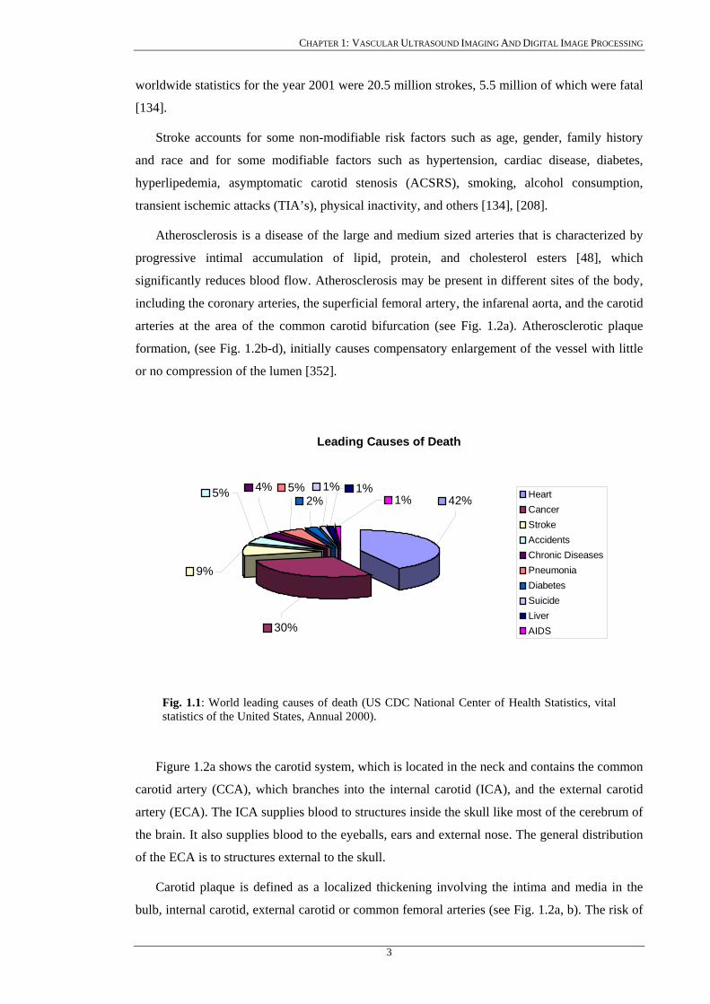
1.1.1 Risk of stroke Figure 1.1 presents the 10 leading causes of death in the world where stroke is the third
leading cause after heart disease (42%), and cancer (30%), with 9% of death incidents
worldwide per year.
According to the 2002 world health report [134] cardiovascular deaths in 2001 accounted
for 36% of all deaths in women, and 30% of all deaths in men, and all predictions suggest
growing figures for the next decade especially for the developing world. It was also reported
from the Heart and Stroke Foundation of Canada [134], that each year in Canada, about 700,000
people develop a stroke, with 500,000 of these being first attacks, and 200,000 recurrent attacks.
Stroke costs the Canadian government more than $40-$50 billion dollars per year. One of the
most important causes of death in the world and the leading cause of serious, long-term
disability in the United States today is cardiovascular disease [134]. Stroke killed 283,000
people in the United States in 2000 and accounted for about one of almost every 14 deaths. The
2
CHAPTER 1: VASCULAR ULTRASOUND IMAGING AND DIGITAL IMAGE PROCESSING
worldwide statistics for the year 2001 were 20.5 million strokes, 5.5 million of which were fatal
[134].
Stroke accounts for some non-modifiable risk factors such as age, gender, family history
and race and for some modifiable factors such as hypertension, cardiac disease, diabetes,
hyperlipedemia, asymptomatic carotid stenosis (ACSRS), smoking, alcohol consumption,
transient ischemic attacks (TIA’s), physical inactivity, and others [134], [208].
Atherosclerosis is a disease of the large and medium sized arteries that is characterized by
progressive intimal accumulation of lipid, protein, and cholesterol esters [48], which
significantly reduces blood flow. Atherosclerosis may be present in different sites of the body,
including the coronary arteries, the superficial femoral artery, the infarenal aorta, and the carotid
arteries at the area of the common carotid bifurcation (see Fig. 1.2a). Atherosclerotic plaque
formation, (see Fig. 1.2b-d), initially causes compensatory enlargement of the vessel with little
or no compression of the lumen [352].
Leading Causes of Death
9%
5% 4% 5%2%
1%1%
1%
30%
42% HeartCancerStrokeAccidentsChronic DiseasesPneumoniaDiabetesSuicideLiverAIDS
Fig. 1.1: World leading causes of death (US CDC National Center of Health Statistics, vital statistics of the United States, Annual 2000).
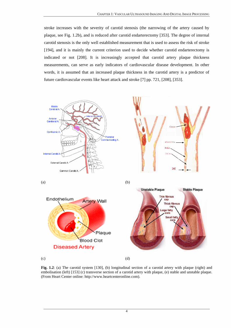
Figure 1.2a shows the carotid system, which is located in the neck and contains the common
carotid artery (CCA), which branches into the internal carotid (ICA), and the external carotid
artery (ECA). The ICA supplies blood to structures inside the skull like most of the cerebrum of
the brain. It also supplies blood to the eyeballs, ears and external nose. The general distribution
of the ECA is to structures external to the skull.
Carotid plaque is defined as a localized thickening involving the intima and media in the
bulb, internal carotid, external carotid or common femoral arteries (see Fig. 1.2a, b). The risk of
3
CHAPTER 1: VASCULAR ULTRASOUND IMAGING AND DIGITAL IMAGE PROCESSING
stroke increases with the severity of carotid stenosis (the narrowing of the artery caused by
plaque, see Fig. 1.2b), and is reduced after carotid endarterectomy [353]. The degree of internal
carotid stenosis is the only well established measurement that is used to assess the risk of stroke
[194], and it is mainly the current criterion used to decide whether carotid endarterectomy is
indicated or not [208]. It is increasingly accepted that carotid artery plaque thickness
measurements, can serve as early indicators of cardiovascular disease development. In other
words, it is assumed that an increased plaque thickness in the carotid artery is a predictor of
future cardiovascular events like heart attack and stroke [7] pp. 721, [208], [353].
(a) (b)
(c) (d)
Fig. 1.2: (a) The carotid system [130], (b) longitudinal section of a carotid artery with plaque (right) and embolisation (left) [153] (c) transverse section of a carotid artery with plaque, (e) stable and unstable plaque. (From Heart Center online: http://www.heartcenteronline.com).
4
CHAPTER 1: VASCULAR ULTRASOUND IMAGING AND DIGITAL IMAGE PROCESSING
Recent studies involving angiography, high-resolution ultrasound, thrombolytic therapy,
plaque pathology, coagulation studies, and more recently molecular biology, have implicated
atherosclerotic plaque rapture as a key mechanism responsible for the development of
cerebrovascular events [369]-[371]. Atherosclerotic disease has two main clinical
manifestations, a) asymptomatic bruits and, b) cerebrovascular syndromes such as amaurosis
fugax, TIA’s or stroke which are often the result of plaque erosion or rupture with subsequent
thrombosis producing occlusion or embolisation [367], [368] (see also Fig. 1.2b).
A stroke occurs usually when the blood supply to parts of the brain is suddenly interrupted
or becomes blocked (Ischemic stroke). Ischemic strokes caused by artery stenosis, account for
approximately 75% of all strokes. This blockage, caused by fatty build-up, is referred to as
atherosclerosis [10], [51], [61], [100], [149]. Atherosclerosis changes the mechanical properties
of the vessel walls and the build up of a plaque making the artery walls stiffer [99]. The plaque
accumulates in the inner lining of blood vessels and results in narrowing and irregularity of the
artery, (see Fig. 1.2b, d). When a blood vessel in the brain bursts, spilling of blood occurs into
the spaces surrounding brain cells and we have a hemorrhagic stroke. For all types of stroke,
treatment must be given immediately, as neuronal death processes quickly after the onset of
symptoms.
The decision to treat narrowing of the carotid artery is not always straightforward. The
potential benefit of the surgery must be weighted against the risk of the surgery. The degree of
stenosis of the carotid artery, the intima-media thickness (IMT), which is the thickness of the
artery walls (see also Fig. 1.2b), and the presence or absence of symptoms are some of the
important factors to consider when taking this decision [71] pp. 334, [194], [208], [266], [353].
Measurements of IMT are better predictors of risk than any combination of conventional risk
factors [149], [322], [372].
Compared to medical therapy alone, surgery (carotid endarterectomy) has been found highly
beneficial for patients who have already had a stroke or experienced the warning signs of a
stroke and have a severe degree of stenosis of 70-99% [208]. Usually these patients are
considered to benefit from a carotid endarterectomy [52], [266]. Based on the evidence of the
North American Symptomatic Carotid Surgery Trial (NASCET), and the European Carotid
Surgery Trial (ECST), for a degree of stenosis of less than 30%, medical therapy is preferred
[208], [353]. For a degree of stenosis between 30% and 70%, the best therapy has not been yet
determined, since the risk/benefit ratio varies between the conditions of the patients. Patients
that are at a high risk for a surgical procedure may be placed on medications to inhibit their
blood from clotting [208], [266].
The primary aim of most digital carotid image-processing techniques is to provide human–
independent aids for assessing the condition of the arteries and assessing the risk of stroke. In
5
CHAPTER 1: VASCULAR ULTRASOUND IMAGING AND DIGITAL IMAGE PROCESSING
normal individuals usually before the age of 40, there is no plaque present in the carotid artery.
As atherosclerosis disease progresses due to various factors [48], [99], [266], [352], the IMT
initially increases diffusely along the artery and then becomes more focal, forming plaques
which gradually obstruct blood flow and causes a lumen stenosis. Furthermore the plaques may
become unstable and rupture to block the artery suddenly if they develop internal pools of lipid
and thrombus covered by a thin fibrous cap (see Fig. 1.2b-d). Lumen stenosis, the degree to
which the vessel is narrowed as a result of plaque growth, is an indirect measure used to
describe the sensitivity of the atherosclerosis, where the IMT and the presence of a plaque, are
direct indicators of the risk of stroke [49], [99], [208]. Accurate measurements and
understanding of the IMT and plaque in the carotid arteries are therefore important for the
assessment and management of the risk of stroke [48], [65], [99], [322].
1.1.2 IMT measurements Measurements of the IMT in the CCA by ultrasound have been used in several clinical trials
[44], [49], [82], [99], [227], [241], [253]-[256], to validate atherosclerosis disease [194], [314],
where measurements from 0.2 mm-2.5 mm were reported. It was shown that increased IMT was
correlated to coronary artery disease and stroke in older adults without a history of
cardiovascular disease [99], [315], [320] and that, a strong correlation of the IMT with
increasing age in both men and women exists, where the estimated change of IMT is 0.009
mm/year. The IMT of patients with a history of cardiovascular disease, such as stroke,
myocardial infraction and angina was increased by 6-12% in comparison to those without
symptomatic cardiovascular disease [320]. Increased IMT was also demonstrated to have a
strong correlation with the presence of atherosclerosis elsewhere in the body. Risk factors like
diabetes, smoking and high blood pressure also may cause an increase of 5-12% in the IMT
[313], [322]. IMT measurements may be therefore used as an indicator of generalized
atherosclerosis and future cardiovascular events.
The degree of the artery stenosis is defined as the percentage of the lumen diameter
reduction relative to a reference vessel diameter. It is usually measured as the difference
between the largest and smallest area of the artery in relation to the largest area [208], [372],
and is defined by the NASCET study as [166]:
⎥⎦
⎤⎢⎣
⎡−
distalICA
ICA
dd
,
min,1100 (1.1.1)
where , is the minimum lumen diameter in the ICA (i.e. at the site of maximal stenosis)
and , is the lumen diameter in a distal diseased free portion of the ICA. In practice,
ICA stenosis is commonly estimated from blood velocity measurements made using Doppler
ultrasound. Although this method has proven effective in identifying stenosis above the
min,ICAd
distalICAd ,
6
CHAPTER 1: VASCULAR ULTRASOUND IMAGING AND DIGITAL IMAGE PROCESSING
threshold for carotid endarterectomy, it is widely considered to be unsuitable for accurate
quantification of disease severity over a wide range of degrees of stenosis [49], [54], [99], [208].
1.1.3 Plaque characteristics Plaque characteristics may also be useful in determining high-risk plaques, which are more
likely to cause thromboembolic events leading to heart attack or stroke [10], [39], [48], [56],
[67]. There is an increasing body of medical research suggesting that differences in the structure
and composition of individual atherosclerotic plaques (plaque morphology), may be linked to
possible future health problems for patients [10], [51], [138], [209], [320], [368], [372]. The
challenge for doctors and technology is to discover a way to identify which plaques can be
referred to as “safe” and which has the potential to break off and threaten the patient’s life.
Homogeneous plaques are characterised by uniformly high- or medium level echoes, smooth
surface, echogenicity, and are associated with stable plaques, whereas heterogeneous plaques
are associated with advance stages of carotid plaque lesion, irregular surface, echolucency, [10],
[51], [320], [322], which are characteristics of a potentially unstable plaque [208] (see also Fig.
1.2d). Echogenic plaques reflect strongly the ultrasound signal, whereas echolucent ones have
less reflectivity ability. It has been shown that echolucent plaques, as evaluated by B-mode
ultrasound, are more likely to lead to the development of neurological events than echogenic
ones [93], [209], [266]. The ultrasonic characteristics of unstable (vulnerable) plaques have
been determined [337], [358] and populations or individuals at increased risk for cardiovascular
events can now be identified [99], [202], [320], [328]. In addition, high-resolution ultrasound
enables the identification of the different ultrasonic characteristics of unstable carotid plaques
associated with amaurosis fugax, TIAs, stroke and different patterns of computer tomography-
brain infraction [337], [358]. This information has provided new insight into the
pathophysiology of the different clinical manifestations of extracranial atherosclerotic
cerebrovascular disease using non-invasive methods.
Different classifications have been proposed in the literature for the characterization of
atherosclerotic plaque morphology, resulting in considerable confusion. For example, plaques
containing medium or high level uniform echoes were classified as homogeneous by Reilly
[303] and correspond closely to Johnson’s dense and calcified plaques [281], to Gray-Weale’s
type 3 and 4 [277] and to Widder’s type I and II plaques [275] (i.e echogenic or hyperechoic).
A recent consensus on carotid plaque characterization has suggested that echodensity should
reflect the overall brightness of the plaque with the term hypoechoic referring to echolucent
plaques [274]. The reference structure to which plaque echodensity should be compared with is
for hypoechoic plaques, blood; for the isoechoic, the sternomastoid muscle; and for the
hyperechoic ones, the bone of the adjacent cervical vertebrae.
7
CHAPTER 1: VASCULAR ULTRASOUND IMAGING AND DIGITAL IMAGE PROCESSING
There is enough evidence published to support the clinical usefulness of ultrasonic plaque
characterization, patients with hypoechoic carotid plaques being at increased risk of stroke.
Polak has recently investigated the association between stroke and ICA plaque echodensity
[266]. Plaque morphology may be subjectively characterized as hypoechoic, isoechoic or
hyperechoic in relation to the surrounding soft tissues. The stroke rate for hypoechoic plaques
was 2.78 times higher than for isoechoic and hyperechoic plaques. In addition to the subjective
characterization of plaques, studies that presented computer assisted plaque characterization
using ultrasound B-mode images of plaques taken from a duplex scanner with fixed instrument
settings including time gain control, have been published. In a study by El-Barghouty et al. the
median of the frequency distribution of gray-scale values of the pixels within the plaque is used
as the measurement of echodensity [209]. It is also reported in the literature, that carotid
endarterectomy in patients with asymptomatic carotid stenosis (ACSRS) will reduce the
incidence of a stroke [208], [322]. However, as a result of the above, a large number of patients
are operated on unnecessarily. For example, twenty patients have to be operated in order to
prevent one stroke episode in 5 years, or 100 patients to prevent one stroke in one year [64],
[353]. Therefore, it is necessary to identify patients with a high risk of developing a stroke (>4%
stroke incidence per annum) who will be considered for carotid endarterectomy, and those
patients with a low risk (<1% per annum), who will be spared from an unnecessary, expensive
and often dangerous operation.
1.2 A brief review of ultrasound imaging
Medical imaging technology has experienced a dramatic change in the last 30 years [4].
Previously only X-ray radiographs were available, which showed the organs as shadows on
photographic film. With the advent of modern computers, new imaging modalities like
computer tomography (CT or CAT computer assisted tomography), magnetic resonance
imaging (MRI), positron emission tomography (PET) and ultrasound, which deliver cross-
sectional images of a patient’s anatomy and physiology, have been developed. Among the
imaging techniques employed are X-ray angiography, X-ray, CT, ultrasound imaging, MRI,
PET, and single photon emission computer tomography (SPECT). MRI and CT have
advantages compared to ultrasound, in the sense that higher resolution and clearer images are
produced.
Imaging techniques have long been used for assessing and treating cardiac [4], [7], [8] and
carotid disease [7], [93], [233]-[235]. Today’s available imaging modalities produce a wide
range of image data types for disease assessment which includes, 2D projection images,
reconstructed three-dimensional (3D) images, 2D slice images, true 3D images, time sequences
of 2D and 3D images, and sequences of 2D interior view (endoluminal) images.
8

CHAPTER 1: VASCULAR ULTRASOUND IMAGING AND DIGITAL IMAGE PROCESSING
The use of ultrasound in the diagnosis and assessment of imaging organs and soft tissue
structures as well as human blood, is well established [4], [44], [50], [55], [136], [141]. Because
of its non-invasive nature and continuing improvements in imaging quality, ultrasound imaging
is progressively achieving an important role in the assessment and characterization of carotid
plaques [51], [126], [255], and assessment of carotid artery disease [55], [56], [136]. The main
disadvantage of ultrasound is that it does not work well in the presence of bone or gas, and the
operator needs a high level of skill in both image acquisition and interpretation to carry out the
clinical evaluation [136]. Standard angiography cannot give reliable information [8], [9], on the
cross-sectional structure of the arteries. This makes it difficult to accurately assess the build-up
of plaque along the artery walls. For some years, B-mode ultrasound imaging or intravascular
ultrasound (IVUS) has emerged and it is used for visualizing carotid plaques and assessment of
plaque characteristics related to the onset of neurological symptoms [57], [73], [217]. To
perform IVUS, one inserts a catheter equipped with an ultrasonic transducer into a vessel of
interest and real-time cross sectional images may be reproduced. However, reproducible
measurements of the severity of the plaque in 2D and 3D ultrasound are made difficult because
of the complex shapes, asymmetry of carotid plaques, and the speckle noise present in
ultrasound images [2], [38], [141]. Furthermore, IVUS is invasive as a catheter is inserted in the
artery and possesses therefore, a certain risk for the patient.
(a) (b) Fig. 1.3: Ultrasound imaging scanners: (a) ATL HDI-3000, (b) ATL HDI-5000 [153].
The use of ultrasound in medicine began during the Second World War in various centres
around the world. The work of Dr. Karl Theodore Dussik in Austria in 1942 [133] on
transmission ultrasound investigation of the brain provides the first published work on medical
ultrasonics. Although other researchers in the USA, Japan, and Europe have also been cited as
pioneers, the work of Professor Ian Donald [200] and his colleagues in Glasgow, in the mid
1950s, did much to facilitate the development of practical technology and applications. This
lead to the wider use of ultrasound in medical practice in subsequent decades.
9
CHAPTER 1: VASCULAR ULTRASOUND IMAGING AND DIGITAL IMAGE PROCESSING
From the mid sixties onwards, the advent of commercially available systems allowed the
wider dissemination of the use of ultrasound. Rapid technological advances in electronics and
piezoelectric materials provided further improvements from bistable to gray-scale images and
from still images to real-time moving images. The technical advances at this time led to a rapid
growth in the applications of ultrasound. The development of Doppler ultrasound [366] had
been progressing alongside the imaging technology but the fusing of the two technologies in
Duplex scanning [50] and the subsequent development of colour Doppler imaging [366]
provided even more scope for investigating the circulation and blood supply to organs, tumours
etc (see also sections 1.2.1, 1.2.2). The advent of the microchip in the seventies and the
subsequent exponential increase in processing power facilitated the development of faster and
more powerful systems incorporating digital beam forming, signal enhancement and new ways
of interpreting and displaying data, such as power Doppler [81], [148] and 3D imaging [45].
Ultrasound has long been recognized as a powerful tool for use in the diagnosis and evaluation
of many clinical entities. Over the past decade, as higher quality less expensive scanners were
developed, ultrasound has proliferated throughout various specialties [65], [66].
Figure 1.3 illustrates the two ultrasound scanners used in this PhD work.
1.2.1 Basic principles of ultrasound Ultrasound is a sound wave with frequency that exceeds 20 . It transports energy and
propagates through several means as a pulsating pressure wave. It is described by a number of
wave parameters such as pressure density, propagation direction, and particle displacement. If
the particle displacement is parallel to the propagation direction then the wave is called
longitudinal or a compression wave. If the particle displacement is perpendicular to the
propagation direction, it is a shear or transverse wave. Interaction of ultrasound waves with
tissue is subject to the laws of geometrical optics. It includes reflection, refraction, scattering,
diffraction, interference and absorption. Except from interference all other interactions reduce
the intensity of the ultrasound beam.
kHz
The main characteristic of an ultrasound wave is the wavelength λ , which is a measure of
the distance between two adjacent maximum or minimum values of a sine curve and frequency
, which is the number of waves per unit of time. The product of these two measures give the
velocity of ultrasound wave propagation,
f
ν , described with the equation λν f= . Ultrasound
techniques are mainly based on measuring the echoes transmitted back from a medium when
sending an ultrasound wave to it. In the echo impulse ultrasound technique, the ultrasound
wave interacts with tissue and blood, and some of the transmitted energy returns to the
transducer to be detected by the instrument. If we know the velocity of propagation in the tissue
being interrogated, we can determine the distance from the transducer at which the interaction
occurred [156]. The characteristics of the return signal (amplitude, phase etc.) provide
10
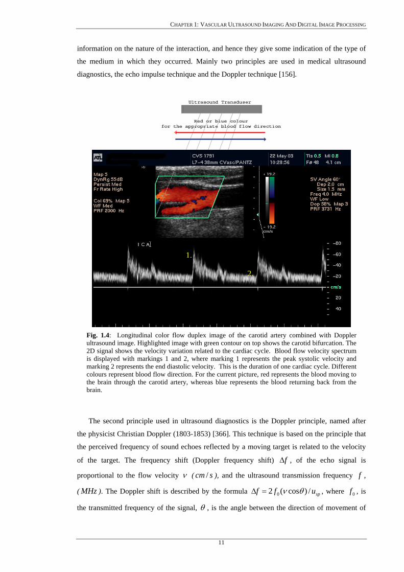
CHAPTER 1: VASCULAR ULTRASOUND IMAGING AND DIGITAL IMAGE PROCESSING
information on the nature of the interaction, and hence they give some indication of the type of
the medium in which they occurred. Mainly two principles are used in medical ultrasound
diagnostics, the echo impulse technique and the Doppler technique [156].
Fig. 1.4: Longitudinal color flowultrasound image. Highlighted ima2D signal shows the velocity variais displayed with markings 1 and marking 2 represents the end diastocolours represent blood flow directthe brain through the carotid arterbrain.
The second principle used in u
the physicist Christian Doppler (18
the perceived frequency of sound e
of the target. The frequency sh
proportional to the flow velocity
( MHz ). The Doppler shift is desc
the transmitted frequency of the si
1.
duplex image of thege with green contour tion related to the card2, where marking 1 rlic velocity. This is thion. For the current piy, whereas blue repre
ltrasound diagnostic
03-1853) [366]. This
choes reflected by a
ift (Doppler frequen
ν ( ), and thescm /
ribed by the formul
gnal, θ , is the angl
11
2.
carotid artery combined with Doppler
on top shows the carotid bifurcation. The iac cycle. Blood flow velocity spectrum epresents the peak systolic velocity and e duration of one cardiac cycle. Different cture, red represents the blood moving to sents the blood returning back from the
s is the Doppler principle, named after
technique is based on the principle that
moving target is related to the velocity
cy shift) f∆ , of the echo signal is
ultrasound transmission frequency , f
a spuff /)cos(2 0 θν=∆ , where , is 0f
e between the direction of movement of
CHAPTER 1: VASCULAR ULTRASOUND IMAGING AND DIGITAL IMAGE PROCESSING
the moving object and the ultrasound beam and , is the speed of sound through tissue that is
approximately 1540 m/s.
spu
In Doppler ultrasound waves are produced by a vibrating crystal using the piezoelectric
effect, whereas the returned echoes are displayed as 2D signal as shown in Fig. 1.4. When blood
flow in a vessel is being examined sound reflections caused by the blood’s corpuscular elements
play a major role. Based on the fact that blood flow velocity varies in different areas of a
vessel, the Doppler signal contains a broad frequency spectrum. In normal ICA the spectrum
varies from 0.5 to 3.5 and is less than 120 when an ultrasound beam of 4 kHz kHz v scm /MHz is used.
1.2.2 Ultrasound modes The two main scanning modes are A- and B-mode. Other modes used are the M-mode,
Duplex ultrasound, colour coded ultrasound, and power Doppler ultrasound, which will be
briefly introduced below.
A-mode refers to amplitude mode scanning, which has mainly a historical interest. In this
mode the strength of the detected echo signal is measured and displayed as a continuous signal
in one direction. A-mode is a line, with strong reflections being represented as an increase of
signal amplitude. This scanning technique has the limitation that the recorded signal is 1D with
limited anatomical information. A-mode is no longer used, especially for the assessment of
cardiovascular disease. Its use is restricted to specialist uses such as ophthalmology in order to
perform very accurate measurements of distance.
B-mode refers to brightness mode. In B-mode echoes are displayed as a 2D gray scale
image. The amplitude of the returning echoes is represented as dots (pixels) of an image with
different gray values as Fig. 1.5 shows. The image is constructed by these pixels line by line.
Advances in B-mode ultrasound have resulted in improved anatomic definition, which has
enable plaque characterization [156], [330].
The M-mode is used in cardiology and it is actually an A-scan plotted against time. The
result is the display of consecutive lines plotted against time. Using this mode, detailed
information may be obtained about various cardiac dimensions and also the accurate timing of
vascular motion.
Moving blood generates a Doppler frequency shift in the reflected sound from insonated red
blood cells and this frequency shift can be used to calculate the velocity of the moving blood,
using the Doppler equation [54], [366]. The invention of gated Doppler ultrasound in the late
1950s allowed velocity sampling at different depths and positions and its subsequent
combination with B-mode real-time ultrasonic imaging led to the development of Duplex
ultrasound. Stenosis in any vessel is characterised by an increase in systolic and diastolic
12

CHAPTER 1: VASCULAR ULTRASOUND IMAGING AND DIGITAL IMAGE PROCESSING
velocities. Several types of Doppler systems are used in medical diagnosis, Continuous Wave
(CW) Doppler, Pulsed Wave (PW) Doppler, Duplex ultrasound and Color Flow Duplex. In CW
Doppler, the machine uses two piezoelectric elements serving as transmitters and receivers.
They transmit ultrasound beams continuously. Because of the continuous way that ultrasound is
being transmitted, no specific information about depth can be obtained. PW Doppler is used in
order to detect blood flow at a specific depth. Sequences of pulses are transmitted to the human
body that are gated for a short period of time in order to receive the echoes. By selecting the
time interval between the transmitted and received pulses, it is possible to examine vessels at a
specific depth.
Fig. 1.5: Ultrasound B-mode longitudinal image of the carotid bifurcation with manually outlined plaque, which is usually confirmed with blood flow image.
Plaque Internal carotid Common carotid Bifurcation External carotid
In colour-coded ultrasound, every pixel is tested for Doppler shift. Using this technique, the
movement of the red blood cells is finally depicted through colour. The final image results by
superimposing the colour-coded image on the B-mode image.
Power Doppler is the depiction of flow, based on the integrated power of the Doppler
spectrum rather than on the mean Doppler frequency. This modality results in an angle, which is
independent of the resulting enhanced sensitivity in flow detection as compared to the colour-
coded Doppler and therefore the detection of low flow is better viewed.
1.2.3 Image quality and resolution The quality of the produced ultrasound image depends on image resolution, axial and
lateral. Resolution is defined as the smallest distance between two points at which they can be
13
CHAPTER 1: VASCULAR ULTRASOUND IMAGING AND DIGITAL IMAGE PROCESSING
represented as distinct. Axial resolution refers to the ability of representing two points that lie
along the direction of ultrasound propagation. It depends on the wavelength of the beam. In B-
mode ultrasound pulses consist of one to two sinusoidal wavelengths, and the axial resolution is
dependent on the wavelength of the waveforms, and lies in the range of the ultrasound
wavelength, λ (0.21 mm). Resolution depends on the frequency of the beam waveforms. Since
this value is reciprocal to the ultrasound frequency ( f/νλ = ), the axial resolution improves
with increasing frequency.
Lateral resolution refers to the ability to represent two points that lie at right angle to the
direction of ultrasound propagation. This is dependent on the width of the ultrasound wave
(beam). To be able to resolve points that lie close together, the width of the ultrasound beam has
to be kept reasonably small and the diameter of the transducer is kept as large as possible (i.e.
small phase-array transducers have a worse lateral resolution than large linear or curved-array
transducers).
In order to achieve the best results in vascular ultrasound imaging, the transmission
frequencies are in the range of 1-10 MHz . The selected frequency depends on the application
domain. For arteries located close to the human skin, frequencies greater than 7.5 MHz are
used, whereas for arteries located deeper in the human body, frequencies from 3-5 MHz are
used. For transcranial applications frequencies less than 2 MHz are used. Though when
selecting a frequency, the user has to keep in mind that axial resolution is proportional to the
ultrasound wavelength; while the intensity of the signal depends on the attenuation of the signal
transmitted through the body, with the higher the frequency the higher the attenuation.
Therefore, there is a trade off between higher resolution ultrasound images at smaller depth and
lower resolution images at higher depths.
1.2.4 Limitations of ultrasound Variability in B-mode images (even when using the same ultrasonic equipment with fixed
settings) does exist [79], [93], [172], [253]. Sources of variability are outlined below:
a) Geometrical and diffraction effects, where spatial compound imaging may be
employed to correct the image [95].
b) Inter-patient variation due to depth dependence and inhomogeneous intervening
tissue, where normalisation techniques may be applied to standardise the image [322]
(see also Chapter 5.3).
c) Speckle is an important factor affecting the quality of ultrasound B-mode imaging. It
is described as an ultrasound textural pattern that varies depending on the type of
biological tissue. The presence of speckle, which is difficult to suppress [131], [141],
[345], may obscure small structures thus degrading the spatial resolution of an
14
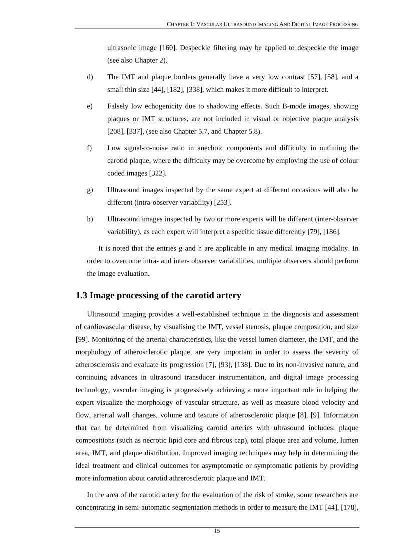
CHAPTER 1: VASCULAR ULTRASOUND IMAGING AND DIGITAL IMAGE PROCESSING
ultrasonic image [160]. Despeckle filtering may be applied to despeckle the image
(see also Chapter 2).
d) The IMT and plaque borders generally have a very low contrast [57], [58], and a
small thin size [44], [182], [338], which makes it more difficult to interpret.
e) Falsely low echogenicity due to shadowing effects. Such B-mode images, showing
plaques or IMT structures, are not included in visual or objective plaque analysis
[208], [337], (see also Chapter 5.7, and Chapter 5.8).
f) Low signal-to-noise ratio in anechoic components and difficulty in outlining the
carotid plaque, where the difficulty may be overcome by employing the use of colour
coded images [322].
g) Ultrasound images inspected by the same expert at different occasions will also be
different (intra-observer variability) [253].
h) Ultrasound images inspected by two or more experts will be different (inter-observer
variability), as each expert will interpret a specific tissue differently [79], [186].
It is noted that the entries g and h are applicable in any medical imaging modality. In
order to overcome intra- and inter- observer variabilities, multiple observers should perform
the image evaluation.
1.3 Image processing of the carotid artery
Ultrasound imaging provides a well-established technique in the diagnosis and assessment
of cardiovascular disease, by visualising the IMT, vessel stenosis, plaque composition, and size
[99]. Monitoring of the arterial characteristics, like the vessel lumen diameter, the IMT, and the
morphology of atherosclerotic plaque, are very important in order to assess the severity of
atherosclerosis and evaluate its progression [7], [93], [138]. Due to its non-invasive nature, and
continuing advances in ultrasound transducer instrumentation, and digital image processing
technology, vascular imaging is progressively achieving a more important role in helping the
expert visualize the morphology of vascular structure, as well as measure blood velocity and
flow, arterial wall changes, volume and texture of atherosclerotic plaque [8], [9]. Information
that can be determined from visualizing carotid arteries with ultrasound includes: plaque
compositions (such as necrotic lipid core and fibrous cap), total plaque area and volume, lumen
area, IMT, and plaque distribution. Improved imaging techniques may help in determining the
ideal treatment and clinical outcomes for asymptomatic or symptomatic patients by providing
more information about carotid athrerosclerotic plaque and IMT.
In the area of the carotid artery for the evaluation of the risk of stroke, some researchers are
concentrating in semi-automatic segmentation methods in order to measure the IMT [44], [178],
15
CHAPTER 1: VASCULAR ULTRASOUND IMAGING AND DIGITAL IMAGE PROCESSING
[227], [241], [253], or to segment the atherosclerotic carotid plaques [64], [184], [191], [220]
from ultrasound images. Other researchers tried to identify the degree of artery stenosis and to
classify arteries as being either as asymptomatic or symptomatic [194], [314], [322]. If
ultrasound shows a stenosis of grater than 70%, magnetic resonance or CT angiography is
recommended [208], [322], [353]. If the results correspond, no further investigation is needed
for surgery. If they do not correspond then a carotid angiogram is required [67], [68].
Figure 1.5 shows a typical longitudinal ultrasound image from a normal adult subject. A
close view of the IMT is shown in Fig. 1.6, with the far wall of the artery being depicted by a
double line pattern, marked with asterisks by an expert. The upper set of asterisks corresponds
to the echogenic lumen-intima and the lower set of asterisks corresponds to the media-
adventitia, which are separated by a sonolucent region. One of our objectives is to apply
despeckle filtering (see Chapter 2), to enhance the boundaries in the image and aid in the
identification, localization, and extraction, of this important ultrasound structure which is
associated with several risk factors for atherosclerosis [99], [202], [320], [328].
Fig. 1.6: Close view of manual measurements of the IMT: (1) 0.9 mm, (2) 0.8 mm, (3) 0.86 mm.
1 2 3
1.3.1 Despeckle filtering Speckle noise, is considered to be the major performance-limiting factor in visual lesion
detection in ultrasound imaging, which makes the lesions difficult to detect and diagnose by the
expert [18]-[34]. Speckle is a multiplicative noise that reduces both image contrast and detail
resolution, degrades tissue texture, reduces the visibility of small low-contrast lesions and
makes continuous structures appear discontinuous. It also limits the effective application (e.g.
edge detection) of automated computer analysis (e.g. volume rendering and 3D display)
algorithms. It is caused by the interference between ultrasound waves reflected from
microscopic scattering through the tissue. A characteristic speckle noise pattern observed in
ultrasound images is shown in Fig. 1.7e and Fig. 1.7f after enlarging a portion of the images in
Fig.1.7a and Fig. 1.7b respectively. Many authors have shown a reduction of lesion detectability
of approximately a factor of eight due to the presence of speckle noise in the image [87], [89],
16
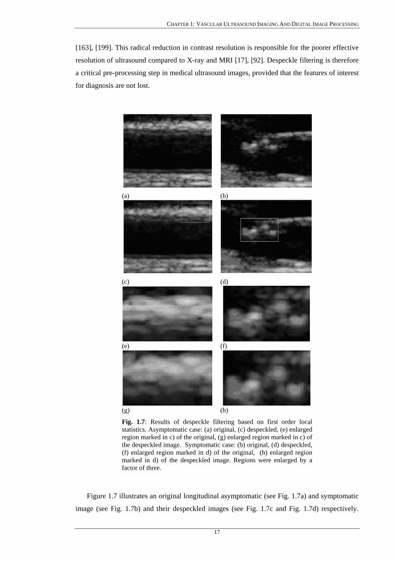
CHAPTER 1: VASCULAR ULTRASOUND IMAGING AND DIGITAL IMAGE PROCESSING
[163], [199]. This radical reduction in contrast resolution is responsible for the poorer effective
resolution of ultrasound compared to X-ray and MRI [17], [92]. Despeckle filtering is therefore
a critical pre-processing step in medical ultrasound images, provided that the features of interest
for diagnosis are not lost.
(a) (b)
(c) (d)
(e) (f)
(g) (h)
Fig. 1.7: Results of despeckle filtering based on first order local statistics. Asymptomatic case: (a) original, (c) despeckled, (e) enlarged region marked in c) of the original, (g) enlarged region marked in c) of the despeckled image. Symptomatic case: (b) original, (d) despeckled, (f) enlarged region marked in d) of the original, (h) enlarged region marked in d) of the despeckled image. Regions were enlarged by a factor of three.
Figure 1.7 illustrates an original longitudinal asymptomatic (see Fig. 1.7a) and symptomatic
image (see Fig. 1.7b) and their despeckled images (see Fig. 1.7c and Fig. 1.7d) respectively.
17
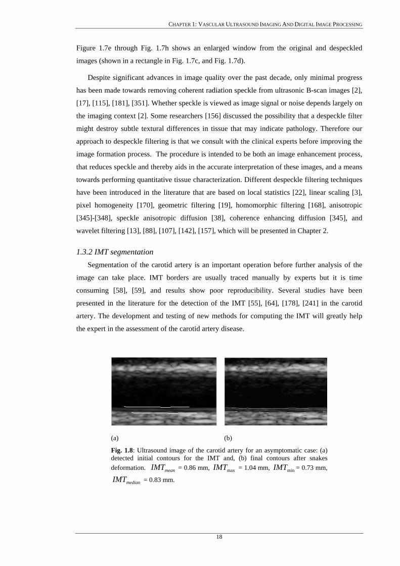
CHAPTER 1: VASCULAR ULTRASOUND IMAGING AND DIGITAL IMAGE PROCESSING
Figure 1.7e through Fig. 1.7h shows an enlarged window from the original and despeckled
images (shown in a rectangle in Fig. 1.7c, and Fig. 1.7d).
Despite significant advances in image quality over the past decade, only minimal progress
has been made towards removing coherent radiation speckle from ultrasonic B-scan images [2],
[17], [115], [181], [351]. Whether speckle is viewed as image signal or noise depends largely on
the imaging context [2]. Some researchers [156] discussed the possibility that a despeckle filter
might destroy subtle textural differences in tissue that may indicate pathology. Therefore our
approach to despeckle filtering is that we consult with the clinical experts before improving the
image formation process. The procedure is intended to be both an image enhancement process,
that reduces speckle and thereby aids in the accurate interpretation of these images, and a means
towards performing quantitative tissue characterization. Different despeckle filtering techniques
have been introduced in the literature that are based on local statistics [22], linear scaling [3],
pixel homogeneity [170], geometric filtering [19], homomorphic filtering [168], anisotropic
[345]-[348], speckle anisotropic diffusion [38], coherence enhancing diffusion [345], and
wavelet filtering [13], [88], [107], [142], [157], which will be presented in Chapter 2.
1.3.2 IMT segmentation Segmentation of the carotid artery is an important operation before further analysis of the
image can take place. IMT borders are usually traced manually by experts but it is time
consuming [58], [59], and results show poor reproducibility. Several studies have been
presented in the literature for the detection of the IMT [55], [64], [178], [241] in the carotid
artery. The development and testing of new methods for computing the IMT will greatly help
the expert in the assessment of the carotid artery disease.
(a) (b)
Fig. 1.8: Ultrasound image of the carotid artery for an asymptomatic case: (a) detected initial contours for the IMT and, (b) final contours after snakes deformation. = 0.86 mm, = 1.04 mm, = 0.73 mm,
= 0.83 mm. meanIMT maxIMT minIMT
medianIMT
18
CHAPTER 1: VASCULAR ULTRASOUND IMAGING AND DIGITAL IMAGE PROCESSING
In the segmentation of an ultrasound image of the carotid artery, interest lies in identifying
and measuring the IMT, determining the presence or absence of a plaque, and determining its
contour provided that a plaque exists. The majority of the proposed segmentation methods
developed, are suitable for delineating the lumen walls, and the IMT. For lumen delineation in
transversal ultrasound imaging, the Hough transform (HT) was initially investigated [148] as
well as to find an initial approximation of the lumen area in the left ventricle [218]. Dynamic
programming [253] and cost function optimization [217] were applied for determining the
optimal vessel wall. In IVUS imaging of the carotid artery for detecting the vessel wall the
following methods were developed: texture based [220], morphology operators [215], optimal
graph searching [72], and dynamic contour modeling [78]. Furthermore, snakes or deformable
models to detect the IMT in 2D [241], and 3D [55], ultrasound images of the carotid artery were
developed. These methods are based on the active contour model first introduced by Kass [243].
In general, the snake-based methods require that the initial snake contour must be specified by
an expert, although recently a method that automatically detects an initial snake contour for the
IMT [115], [252], [338], was introduced, as a first step towards the automated segmentation of
the IMT and plaque in the carotid artery images.
Figure 1.8a shows a longitudinal ultrasound image of the CCA with computed initial
contours at the far wall, of the intima and the adventitia layers based on despeckle filtering and
morphology operators, whereas Fig. 1.8b shows the final result after the two contours were
deformed using the Williams&Shah snakes segmentation method proposed in Chapter 3.
1.3.3 Plaque segmentation As it has been mentioned in the previous section on IMT segmentation, the segmentation of
an ultrasound image of the carotid artery necessitates the need to identify and measure the IMT
and determine the presence or absence of a plaque. If there is a plaque its contour should be
determined. Although in ultrasound imaging, different segmentation methods were developed
for IMT segmentation, no method was developed for segmenting the atherosclerotic carotid
plaque in longitudinal ultrasound images.
Traditionally, X-ray angiography is used for measuring manually the percentage of stenosis
of the carotid artery. However this measure may not be reliably estimated because this modality
depicts only the lumen of the artery [10], [208], [322], [372]. Furthermore, X-ray angiography is
not capable of visualising the vessel wall and cannot determine the size or composition of the
atherosclerotic plaque [71], [93], [100], [320]. The use of ultrasound significantly helps in
determining the size or composition of atherosclerotic carotid plaque.
19

CHAPTER 1: VASCULAR ULTRASOUND IMAGING AND DIGITAL IMAGE PROCESSING
(a) (b)
Fig. 1.9: Ultrasound image of the carotid artery: (a) plaque initial contour estimation, and (b) the final plaque contour after the snakes deformation.
Some researchers have attempted to segment the carotid plaque from MRI, by using active
contours [191], and dynamic programming [321]. Others have used a graph-searching approach
to detect the wall and plaque in IVUS images [72]. Figure 1.9a shows an ultrasound image of
the carotid artery, where an initial contour for the plaque was estimated, whereas in Fig. 1.9b the
final plaque contour is shown after the deformation by the Williams&Shah snakes segmentation
method proposed in Chapter 3.
1.4 Original aspects of the work
The original aspects of this work are the following:
a) Quantitative image quality evaluation: Investigate the usefulness of quantitative
quality evaluation metrics in ultrasound imaging of the carotid artery. For this task we
have evaluated the quality of ultrasound imaging of the carotid artery on two different
ultrasound scanners, the HDI ATL-3000 and the HDI ATL-5000, before and after de-
speckle filtering, and after despeckle filtering and image normalization. Statistical and
texture analysis was carried out on the above-mentioned preprocessed images and
these findings were compared with the visual perception, carried out by two experts.
Results showed that the normalised despeckled images were rated visually better on
both scanners. Also, the texture analysis evaluation showed that the normalised
despeckled images were better on both scanners.
b) Despeckle filtering: Develop and evaluate a number of despeckle filtering methods for
the pre-processing of carotid ultrasound images. For this purpose, a total of 11
despeckle filters presented in Chapter 2, were developed based on local statistics,
median filtering, linear scaling, pixel homogeneity, geometric filtering, logarithmic
filtering, homomorphic filtering, anisotropic diffusion, speckle anisotropic diffusion,
non-linear coherence diffusion and wavelet filtering. Despeckle filtering was
evaluated on 440 (220 asymptomatic and 220 symptomatic) longitudinal ultrasound
20
CHAPTER 1: VASCULAR ULTRASOUND IMAGING AND DIGITAL IMAGE PROCESSING
images of the carotid artery bifurcation. Furthermore, despeckle filtering evaluation
was investigated using the visual perception by two experts, statistical and texture
analysis, as well as image quality evaluation metrics. Results showed that a despeckle
filter based on local statistics (lsmv) improved the class separation between the
asymptomatic and the symptomatic classes, gave only a marginal improvement in the
percentage of correct classifications success rate, and improved the visual assessment
by the experts. It was also found that the lsmv despeckle filter can be used for
despeckling asymptomatic images where the expert is interested mainly in the plaque
composition and texture analysis, whereas a geometric despeckle filter (gf4d) can be
used for despeckling of symptomatic images where the expert is interested in
identifying the degree of stenosis and the plaque borders.
c) IMT snakes segmentation: Develop and evaluate a new segmentation method to
extract the IMT borders and measure the IMT from longitudinal ultrasound carotid
artery images. The IMT snakes segmentation method, developed in this work is based
on the Williams&Shah [124] snake and utilises an automatic initial contour
estimation, so that the snake will be placed in a close proximity to the borders of
interest. The initial contour estimation was performed on the ultrasound image after
despeckle filtering and normalisation. Unlike classical based algorithms where experts
place the initial contour manually we estimate the initial snake contour automatically
using morphology operators. Segmentation was carried out on the original,
despeckled, normalized and normalized despeckled images. We have tested and
validated the Williams&Shah IMT snakes segmentation method on 100 images of the
carotid artery based on univariate statistical analysis, correlation and regression
analysis, and on visual perception by two experts. The IMT mean standard
deviation snakes segmentation results were 0.7
±
± 0.14 mm, 0.69 0.13 mm,
0.67
±
± 0.13 mm, 0.68± 0.12 mm, for the original, despeckled, normalized, and
normalized despeckled images respectively. The manual ± standard deviation results
for the first expert were, 0.67± 0.16 mm, 0.68± 0.17 mm, and for the second expert
were, 0.65 0.18 mm, 0.61± ± 0.17 mm on the original and normalized images
respectively. The results showed that there was no significant difference between all
the snakes segmentation measurements and the manual measurements. Furthermore
snakes segmentation results were more reproducible than the manual measurements
on the normalized despeckled ultrasound images.
d) Plaque snakes segmentation: Develop and evaluate four different plaque snakes
segmentation methods on 80 ultrasound images of the carotid artery based on the
Williams&Shah [124], the Balloon [333], the Lai&Chin [248], and the GVF [116]
algorithms to extract the plaque borders from ultrasound longitudinal carotid artery
21
CHAPTER 1: VASCULAR ULTRASOUND IMAGING AND DIGITAL IMAGE PROCESSING
images. The four different plaque snakes segmentation methods, in order to find the
initial plaque boundaries, utilise an automatic initial contour estimation and place it as
close as possible to the borders of interest. The plaque snakes segmentation method,
estimated the initial plaque contour, using the B-mode and the blood flow images. The
initial contour was mapped on the original B-mode image, which was despeckled and
normalized. The contour was then deformed by the snake for best fit of the plaque
boundaries. We have validated the four plaque snakes segmentation methods using the
manual measurements made by a vascular expert, the performance of the algorithms,
and ROC (receiver operating characteristics) analysis. The plaque segmentation
results showed that, the Lai&Chin segmentation method that is based on variable
snake parameters, gave results closest to the manual delineation procedure, compared
with the results given by the Williams&Shah, Balloon, and the GVF, snakes
segmentation methods. Specifically the Lai&Chin segmentation method, gave a better
true positive fraction (82.7%), and true negative fraction (80.89%), a better kappa
index (80.66%), and overlap index (69.3%). Furthermore, the Lai&Chin snakes
segmentation method gave the best sensitivity, R, and precision, P with 0.8270 and
0.9338 respectively. The Balloon snakes segmentation method gave the best
specificity, Sp, and a goodness measure F, with 0.946 and 0.8882 respectively. The
area below the ROC was 0.88, 0.85, 0.82, and 0.76 for the Lai&Chin, Balloon,
Williams&Shah, and GVF snakes segmentation method respectively, with the largest
area under the ROC curve obtained by the Lai&Chin snakes segmentation method.
e) Integrated system for the despeckling and segmentation of atherosclerotic carotid
images: The proposed system should be designed, developed and implemented
supporting the processing of atherosclerotic carotid plaque images based on the
algorithms mentioned in a)-d). It should be simple and user-friendly, recording all
processing and analysis steps carried out, illustrate to the expert the image analysis
and measurements results, save the results in a database, display results of different
methods and run in real time.
It should be emphasised that to the best of our knowledge no other studies carried out a
comparative despeckle filtering on ultrasound imaging of the carotid artery, no other studies
performed such a large scale analysis for the IMT segmentation as well as no other study
performed a plaque segmentation on longitudinal ultrasound images of the carotid artery.
1.5 Guide to Thesis Contents
Chapter 2 introduces the theoretical concepts of the despeckle filters used in this work,
where a multiplicative speckle noise model suitable for ultrasound images, is derived.
22
CHAPTER 1: VASCULAR ULTRASOUND IMAGING AND DIGITAL IMAGE PROCESSING
Chapter 3 presents the theoretical background of the IMT and plaque snakes segmentation
method in ultrasound images of the carotid artery. A literature review of the IMT and plaque
segmentation techniques is presented whereas a segmentation technique for the IMT and the
plaque borders is developed using the Williams&Shah snake model [124]. The theoretical and
mathematical derivation of the Williams&Shah, Balloon [333], Lai&Chin [248], and GVF
[116], snakes segmentation methods, are furthermore explained. Finally a review on different
snake initialization procedures used in the literature is presented.
Chapter 4 deals with the issue of image and segmentation quality evaluation in ultrasound
images of the carotid artery. A number of evaluation metrics are presented for evaluating the
despeckle and segmentation methods. Despeckle filtering is evaluated quantitatively using
image quality evaluation metrics, and texture analysis, whereas segmentation is evaluated using
the ROC curve analysis.
Chapter 5 presents the methodology of our work where the ultrasound scanners, material
used, the process of image acquisition, and image normalization, is presented respectively.
Furthermore, the process of generating an artificial carotid image, and the visual, and texture
analysis evaluation for the despeckle filtering is presented. The protocols for the manual and the
snakes segmentation for the IMT, and plaque are furthermore explained, whereas, statistical
metrics are proposed for the segmentation evaluation.
Chapter 6 presents the results of our study with a comparison and discussion of the different
despeckle filters. Furthermore, the segmentation results for the IMT and plaque in ultrasound
images of the carotid artery are presented, using the evaluation metrics presented in Chapter 4.
The evaluation of the proposed despeckle, and segmentation methods, was based on real
ultrasound images of the carotid artery.
Discussion of findings of this work are reported in Chapter 7, together with a discussion of
the despeckle filtering and segmentation results presented in Chapter 6. A comparison with
other studies is attempted whenever possible. Based on the results obtained in this study, a short
description of a proposed system is given.
The last Chapter, Chapter 8, presents the concluding remarks and gives suggestions for
future work.
Five Appendices provide additional information. Appendix I presents the theory on speckle
statistics. Appendix II presents procedures for optical perception evaluation. Appendix III
includes the 55 texture features used in this work for texture analysis. Appendix IV describes
the mathematical derivation of the snakes segmentation algorithm. Finally, Appendix V
includes the publications made during this work.
23

CHAPTER II: DESPECKLE FILTERING
Chapter 2
Despeckle Filtering
24
CHAPTER II: DESPECKLE FILTERING
CHAPTER 2: DESPECKLE FILTERING
Noise and artefacts can cause signal and image degradations for many medical image
modalities. Different image modalities exhibit distinct types of degradation. Radiographs often
exhibit low contrast while images formed with coherent energy, such as ultrasound, suffer from
speckle noise. Image degradation can have a significant impact on image quality and thus affect
human interpretation and the accuracy of computer-assisted methods. Poor image quality often
makes feature extraction, analysis, recognition, and quantitative measurements problematic and
unreliable. Therefore, image despeckling is a very important task, which motivated a
considerable amount of research in medical imaging.
In this Chapter we introduce speckle noise as a major factor limiting the visual perception
and processing of ultrasound images. A mathematical speckle model is introduced, where the
statistics of speckle noise are presented, taking into consideration the log-compression of the
ultrasound image, which is performed in order to match the image into the display device.
Based on this speckle model, a number of despeckling techniques are derived and explained in
detail. Specifically the following categories of despeckle filtering techniques are presented:
local statistics, median filtering, linear scaling, homogeneity, geometric filtering, logarithmic,
homomorphic, anisotropic diffusion, and wavelet filtering.
2.1 Introduction
Ultrasound images show a granular appearance known as speckle, which is a form of locally
correlated multiplicative noise corrupting medical ultrasound imaging making visual
observation and image analysis difficult [163], [164], [339]-[341]. The presence of speckle
noise in ultrasound images has been documented since the early 1970’s where researchers such
as Goodman [163], Burckhardt [164], and Wagner [339], described its fundamentals and its
statistical properties. Speckle noise is the primary factor, which limits the contrast resolution in
diagnostic ultrasound imaging, thereby limiting the detectability of small, low contrast lesions
and making the ultrasound images generally difficult, even for an expert to interpret [22]-[28],
[163], [164], [339]. Speckle noise also limits the effective application of image processing and
analysis algorithms (i.e. edge detection, segmentation) and display in 2D and volume rendering
in 3D. Even expert radiologists with sufficient experience may not often draw useful
conclusions from the images [87], [131], [132]. From an engineering point of view, speckle is
most often considered a dominant source of noise in ultrasound imaging and therefore should be
filtered out [25], [87], [107], [132], [152], [345]. For images that contain speckle, enhancing the
image by removing the speckle without affecting important features is the goal.
25
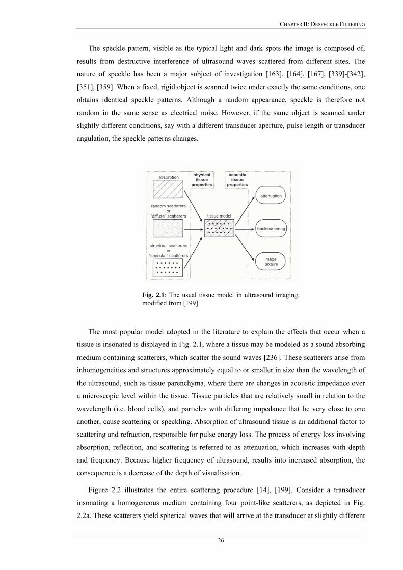
CHAPTER II: DESPECKLE FILTERING
The speckle pattern, visible as the typical light and dark spots the image is composed of,
results from destructive interference of ultrasound waves scattered from different sites. The
nature of speckle has been a major subject of investigation [163], [164], [167], [339]-[342],
[351], [359]. When a fixed, rigid object is scanned twice under exactly the same conditions, one
obtains identical speckle patterns. Although a random appearance, speckle is therefore not
random in the same sense as electrical noise. However, if the same object is scanned under
slightly different conditions, say with a different transducer aperture, pulse length or transducer
angulation, the speckle patterns changes.
Fig. 2.1: The usual tissue model in ultrasound imaging, modified from [199].
The most popular model adopted in the literature to explain the effects that occur when a
tissue is insonated is displayed in Fig. 2.1, where a tissue may be modeled as a sound absorbing
medium containing scatterers, which scatter the sound waves [236]. These scatterers arise from
inhomogeneities and structures approximately equal to or smaller in size than the wavelength of
the ultrasound, such as tissue parenchyma, where there are changes in acoustic impedance over
a microscopic level within the tissue. Tissue particles that are relatively small in relation to the
wavelength (i.e. blood cells), and particles with differing impedance that lie very close to one
another, cause scattering or speckling. Absorption of ultrasound tissue is an additional factor to
scattering and refraction, responsible for pulse energy loss. The process of energy loss involving
absorption, reflection, and scattering is referred to as attenuation, which increases with depth
and frequency. Because higher frequency of ultrasound, results into increased absorption, the
consequence is a decrease of the depth of visualisation.
Figure 2.2 illustrates the entire scattering procedure [14], [199]. Consider a transducer
insonating a homogeneous medium containing four point-like scatterers, as depicted in Fig.
2.2a. These scatterers yield spherical waves that will arrive at the transducer at slightly different
26
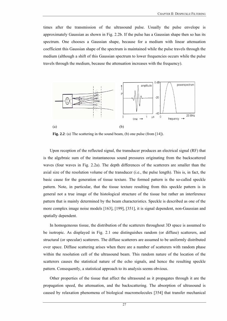
CHAPTER II: DESPECKLE FILTERING
times after the transmission of the ultrasound pulse. Usually the pulse envelope is
approximately Gaussian as shown in Fig. 2.2b. If the pulse has a Gaussian shape then so has its
spectrum. One chooses a Gaussian shape, because for a medium with linear attenuation
coefficient this Gaussian shape of the spectrum is maintained while the pulse travels through the
medium (although a shift of this Gaussian spectrum to lower frequencies occurs while the pulse
travels through the medium, because the attenuation increases with the frequency).
(a) (b)
Fig. 2.2: (a) The scattering in the sound beam, (b) one pulse (from [14]).
Upon reception of the reflected signal, the transducer produces an electrical signal (RF) that
is the algebraic sum of the instantaneous sound pressures originating from the backscattered
waves (four waves in Fig. 2.2a). The depth differences of the scatterers are smaller than the
axial size of the resolution volume of the transducer (i.e., the pulse length). This is, in fact, the
basic cause for the generation of tissue texture. The formed pattern is the so-called speckle
pattern. Note, in particular, that the tissue texture resulting from this speckle pattern is in
general not a true image of the histological structure of the tissue but rather an interference
pattern that is mainly determined by the beam characteristics. Speckle is described as one of the
more complex image noise models [163], [199], [351], it is signal dependent, non-Gaussian and
spatially dependent.
In homogeneous tissue, the distribution of the scatterers throughout 3D space is assumed to
be isotropic. As displayed in Fig. 2.1 one distinguishes random (or diffuse) scatterers, and
structural (or specular) scatterers. The diffuse scatterers are assumed to be uniformly distributed
over space. Diffuse scattering arises when there are a number of scatterers with random phase
within the resolution cell of the ultrasound beam. This random nature of the location of the
scatterers causes the statistical nature of the echo signals, and hence the resulting speckle
pattern. Consequently, a statistical approach to its analysis seems obvious.
Other properties of the tissue that affect the ultrasound as it propagates through it are the
propagation speed, the attenuation, and the backscattering. The absorption of ultrasound is
caused by relaxation phenomena of biological macromolecules [354] that transfer mechanical
27
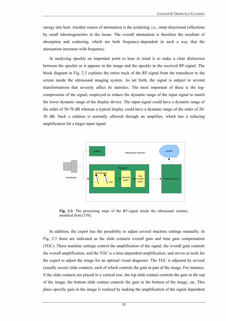
CHAPTER II: DESPECKLE FILTERING
energy into heat. Another source of attenuation is the scattering, i.e., omni directional reflections
by small inhomogeneities in the tissue. The overall attenuation is therefore the resultant of
absorption and scattering, which are both frequency-dependent in such a way that the
attenuation increases with frequency.
In analyzing speckle an important point to bear in mind is to make a clear distinction
between the speckle as it appears in the image and the speckle in the received RF-signal. The
block diagram in Fig. 2.3 explains the entire track of the RF-signal from the transducer to the
screen inside the ultrasound imaging system. As set forth, the signal is subject to several
transformations that severely affect its statistics. The most important of these is the log-
compression of the signal, employed to reduce the dynamic range of the input signal to match
the lower dynamic range of the display device. The input signal could have a dynamic range of
the order of 50-70 dB whereas a typical display could have a dynamic range of the order of 20-
30 dB. Such a relation is normally affected through an amplifier, which has a reducing
amplification for a larger input signal.
Scan converter
pulser screenUltrasound Scanner
Receiver
transducer demodulation
Logcompression
Overall gain
TGC
Fig. 2.3: The processing steps of the RF-signal inside the ultrasound scanner, modified from [156].
In addition, the expert has the possibility to adjust several machine settings manually. In
Fig. 2.3 these are indicated as the slide contacts overall gain and time gain compensation
(TGC). These machine settings control the amplification of the signal, the overall gain controls
the overall amplification, and the TGC is a time-dependent amplification, and serves as tools for
the expert to adjust the image for an optimal visual diagnosis. The TGC is adjusted by several
(usually seven) slide contacts, each of which controls the gain in part of the image. For instance,
if the slide contacts are placed in a vertical row, the top slide contact controls the gain in the top
of the image, the bottom slide contact controls the gain in the bottom of the image, etc. This
place specific gain in the image is realized by making the amplification of the signal dependent
28
CHAPTER II: DESPECKLE FILTERING
on the exact time that the sound reflection is received. Since the place where a pixel is put on
the screen is dependent on this time instant, the time dependent amplification of the received
signal converts to a place dependent change in gray value of the pixels on the screen.
In the following section a speckle model, suitable for ultrasound images is derived, whereas
in section 2.3 the despeckle filters derived in this work, are explained.
2.2 Speckle modeling in ultrasound images
The despeckle filtering methods described in this work are based on the noise model as
proposed in [351], which is adopted for speckle noise in ultrasound B-mode carotid artery
images. The speckle noise model may be approximated as multiplicative if the envelope signal
which is received at the output of the beamformer of the ultrasound imaging system, is captured
before logarithmic compression and may be defined as:
jijijiji anxz ,,,, += , Nij ∈, (2.2.1)
where , represents the noisy pixel in the middle of the moving window, , represents the
noise-free pixel, , and , represent the multiplicative and additive noise (independent of
, with mean 0), respectively, and , are the indices of the spatial locations that belong in
the 2D space of real numbers,
jiz , jix ,
jin , jia ,
jiz , ji,
2, ℜ∈ji . This model is particularly suitable for our purpose, as
it can be applied on the images as displayed by the ultrasound machine rather than the envelope
detected echo signal [271], [345], [351]. Despeckling consists in estimating the true intensity of
, as a function of the intensity of the pixel , and some local statistics calculated on a
neighbourhood of this pixel. Wagner et al. [339] has shown that the histogram of amplitudes
within the resolution cells of the envelope detected RF-signal backscattered from a uniform area
with a sufficiently high scatterer density has a Rayleigh distribution with
jix , jiz ,
µ proportional to the
σ , )91.1/( =σµ . This implies that speckle could be modelled as multiplicative noise.
However, the signal processing stages inside the scanner, (mainly the logarithmic compression)
in order to adjust the large echo dynamic range (50-70dB) to the 8-bits of the digitization in the
scan converter, modify the statistics of the original signal. The model in (2.2.1) has been shown
to be valid for images as displayed by the ultrasound scanner in studies [341], [345], [355],
[360]. In particular it should be noted, that speckle is no longer multiplicative in the sense that
on homogeneous regions, where , can be assumed constant, the mean is proportional to the
variance , rather than the standard deviation
jix ,
)( 2σµ ≈ )( σµ ≈ , [141], [345], [349], [351]. In
this respect, the speckle index, C, which will be presented in Chapter 4 (see (4.9)), will be for
the log-compressed ultrasound images, . µσ /2=C
29
CHAPTER II: DESPECKLE FILTERING
The variance of the speckle noise, , may be calculated from the logarithmically
compressed image, by computing the average noise variance over a number of windows with
dimensions considerable larger than the filtering window. In each window the noise variance is
computed as [351]:
2nσ
∑=
=p
ippn g
1
22 /σσ (2.2.2)
where , and 2pσ pg , are the variance and the mean of the noise in the selected windows
respectively and p , is the index covering all windows in the whole image [345], [351]. We
may therefore calculate the variance of the speckle noise, , from the noise image
characteristics, namely from
2nσ
pg , and , over the image. The speckle noise variance, ,
will be used in some of the despeckle filters which are introduced in the following Chapters.
2pσ 2
nσ
As shown earlier, nonlinear processing such as logarithmic compression, employed on
ultrasound echo images, affects the speckle statistics in such a way that the local mean becomes
proportional to the local variance rather than the standard deviation. More specifically,
logarithmic compression affects the high intensity tail of the Rayleigh and Rician PDFs more
than the low intensity part. As a result the speckle noise becomes very close to white Gaussian
noise corresponding to the uncompressed Rayleigh signal [351]. The envelope at the output of
the beamformer before logarithmic compression, may thus be approximated as shown in (2.2.1).
Since the effect of additive noise, such as sensor noise, is considerably smaller and less
significant compared with that of the multiplicative noise component [141], [345] such as:
(2
,
2
, jiji n<<α ) (2.2.3)
then the filters utilizing first order statistics such as the variance and the mean of the
neighborhood, may be derived from (2.2.1) with the following multiplicative model as:
jijiji nxz ,,, ≈ . (2.2.4)
The logarithmic amplification transforms the model in (2.2.4) into the classical signal in
additive noise form as:
)log()log()log( ,,, jijiji nxz += , (2.2.5a)
. (2.2.5b) jijiji nlfg ,,, +=
For the rest of the work the term , which is the observed pixel on the ultrasound
image display after logarithmic compression, is denoted as , and the terms , and
)log( , jiz
jig , )log( , jix
30

CHAPTER II: DESPECKLE FILTERING
)log( , jin , which are the noise free pixel and noise component after logarithmic compression, as
, and , respectively (see Eq. 2.2.5b). jif , jinl ,
2.3 Despeckle filters
Despeckling is always a trade-off between noise suppression and loss of information,
something that experts are very concerned about. It is therefore attractive to keep as much of
important information as possible. Despeckle filtering can be used as a pre-processing step for
image segmentation [115], or image registration [81], techniques. By suppressing the speckle
the performance of these techniques can be improved.
The despeckle filters originated from the Synthetic Aperture Radar (SAR) community [18],
[22], [31]-[36], [107]. These techniques have later been applied to ultrasound imaging since the
early 1980’s [167], which may be described with the same statistical model as the one
describing the SAR images. The most widely used filters in SAR and ultrasound imaging
include the Frost [27], [28], Lee [22]-[26], and the Kuan [29], [30].
Most adaptive filters only use local statistical information related to the central pixel to be
filtered [2], [21]-[26], [115]. Some additional information may be used from the despeckle
window (see next subsection) to improve despeckling, by utilising the higher order statistics of
the image. Many adaptive despeckling methods have been proposed, such as the Lee filter [22]-
[26], Frost [27], [28], Kuan [29], [30], and Lopes [31], [32]. Furthermore, the Gaussian filter
function [84] has been used for despeckling but it was shown [83], that this form of filtering is
not suitable for speckle noise, as it does not take into consideration the true positions of object
boundaries. However, the full removal of speckle noise without losing any information in
ultrasound images is still a long way off. When additionally edges are present in the filtering
window, the central pixel gray level replaced by the information from all its neighbourhood
pixels will not be correct. Lee has therefore introduced [25] an edge detector, which was
implemented in his old algorithm version [22].
Since the early 1980’s, various researchers have presented the progress that has been made
in quantitative ultrasound imaging and reported techniques that have been applied on ultrasound
images for despeckling [167]. The majority of the despeckling filtering techniques presented in
the literature, have certain limitations that can be briefly summarised as follows:
a) They are sensitive to the size and shape of the window [2], [23], [30], [38], [115],
[345]. The use of different window sizes will greatly affect the quality of the
processed images. If the window is too large over smoothing will occur, subtle
details of the image will be lost in the filtering process and edges will be blurred. A
small window will decrease the smoothing capability of the filter and will not reduce
31
CHAPTER II: DESPECKLE FILTERING
speckle noise thus making the filter not effective. In homogenous areas, the larger the
window size, the more efficient is the filter in reducing the speckle noise. In
heterogeneous areas the smaller the window size, the more it is possible to keep
subtle image details unchanged. Our experiments showed that a 7x7 window size is a
fairly good choice. The images presented in this work have been processed either by
7x7 or by 5x5 pixel windows.
b) Some of the despeckling methods, based on window approaches [2], [19], [22], [131],
require thresholds to be used in the filtering process, which have to be estimated
empirically. The inappropriate choice of a threshold may lead to averaging filtering
and noisy boundaries from leaving the sharp features unfiltered [19], [22], [131].
c) Most of the existing despeckle filters do not enhance edges but they only inhibit
smoothing near the edges. When an edge is contained in the filtering window, the
coefficient of variation will be high and smoothing will be inhibited. Therefore,
speckle in the neighbourhood of an edge will remain after filtering. They are not
directional in the sense that in the presence of an edge, all smoothing is precluded.
Instead of inhibiting smoothing in directions perpendicular to the edge, smoothing in
directions parallel to the edge is allowed. d) Different evaluation criteria for evaluating the performance of despeckle filtering
were used in different studies. Although most of the studies used quantitative criteria
like the MSE and the speckle index, C, there are additional quantitative criteria, like
texture analysis and classification, image quality evaluation metrics, and experts
assessment that could be investigated (see Chapter 4).
Speckle reduction techniques that have been proposed in the literature and have also been
used in our study, are shown in Table 2.1 and are summarized under the following categories:
local statistics, median filtering, linear scaling, homogeneity, geometric, logarithmic,
homomorphic, anisotropic diffusion, and wavelet filtering. These filters are presented in greater
detail in the next section. Some of the local statistic filters are the Lee [22]-[26], the Frost [27],
[28] and the Kuan [29], [30] filters. The Lee and Kuan filters have the same structure, where
the Kuan is a generalization of the Lee filter.
Both filters form an output image by computing a linear combination of the central pixel
intensity in a filter window with the average intensity of the window and a coefficient of
variation inside the moving window. Kuan considered a multiplicative speckle model and
designed a linear filter, based on the minimum-mean-square error (MMSE) criterion, optimal
when the intensity image is Gaussian distributed. The Lee [22] MMSE filter was a particular
case of the Kuan filter based on a linear approximation made for the multiplicative noise model.
32
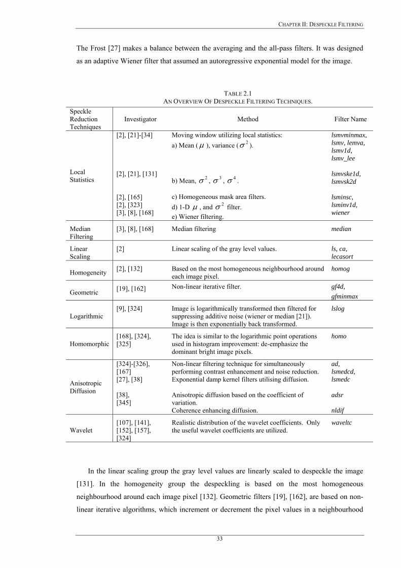
CHAPTER II: DESPECKLE FILTERING
The Frost [27] makes a balance between the averaging and the all-pass filters. It was designed
as an adaptive Wiener filter that assumed an autoregressive exponential model for the image.
TABLE 2.1 AN OVERVIEW OF DESPECKLE FILTERING TECHNIQUES.
Speckle Reduction Techniques
Investigator Method Filter Name
Local Statistics
[2], [21]-[34] [2], [21], [131] [2], [165] [2], [323] [3], [8], [168]
Moving window utilizing local statistics: a) Mean (µ ), variance ( ). 2σ b) Mean, , , . 2σ 3σ 4σ c) Homogeneous mask area filters. d) 1-D µ , and filter. 2σe) Wiener filtering.
lsmvminmax, lsmv, lemva, lsmv1d, lsmv_lee lsmvske1d, lsmvsk2d lsminsc, lsminv1d, wiener
Median Filtering
[3], [8], [168] Median filtering median
Linear Scaling
[2] Linear scaling of the gray level values. ls, ca, lecasort
Homogeneity [2], [132] Based on the most homogeneous neighbourhood around each image pixel.
homog
Geometric [19], [162] Non-linear iterative filter. gf4d, gfminmax
Logarithmic [9], [324] Image is logarithmically transformed then filtered for
suppressing additive noise (wiener or median [21]). Image is then exponentially back transformed.
lslog
Homomorphic [168], [324], [325]
The idea is similar to the logarithmic point operations used in histogram improvement: de-emphasize the dominant bright image pixels.
homo
Anisotropic Diffusion
[324]-[326], [167] [27], [38] [38], [345]
Non-linear filtering technique for simultaneously performing contrast enhancement and noise reduction. Exponential damp kernel filters utilising diffusion. Anisotropic diffusion based on the coefficient of variation. Coherence enhancing diffusion.
ad, lsmedcd, lsmedc adsr nldif
Wavelet [107], [141], [152], [157], [324]
Realistic distribution of the wavelet coefficients. Only the useful wavelet coefficients are utilized.
waveltc
In the linear scaling group the gray level values are linearly scaled to despeckle the image
[131]. In the homogeneity group the despeckling is based on the most homogeneous
neighbourhood around each image pixel [132]. Geometric filters [19], [162], are based on non-
linear iterative algorithms, which increment or decrement the pixel values in a neighbourhood
33
CHAPTER II: DESPECKLE FILTERING
based upon their relative values. The method of homomorphic filtering [168], [325], is similar
to the logarithmic point operation used in histogram improvement, where dominant bright pixels
are de-emphasised. In the homomorphic filtering the image is logarithmically transformed, the
FFT of the image is calculated, then despeckled, the inverse FFT is calculated, and finally
exponentially transformed back.
Some other despeckle filtering methods, such as anisotropic diffusion [37], [38], [326],
[344]-[347], speckle reducing anisotropic diffusion [38], and coherence anisotropic diffusion
[345], presented recently in the literature, are non-linear filtering techniques for simultaneously
performing contrast enhancement and noise reduction by utilising the coefficient of variation
[38]. Furthermore, in the wavelet category, filters for suppressing the speckle noise by making
use of a realistic distribution of the wavelet coefficients [107], [141], [157], [348]-[350], where
only the useful wavelet coefficients are utilised, were documented. Wavelet methods involve a
pre-processing step consisting of a logarithmic transform to separate the noise from the original
image. Then different wavelet shrinkage approaches are employed, based on Donoho’s work
[350].
Some other researchers have tried in the past to despeckle SAR images by averaging of
uncorrelated images obtained from different spatial positions [343]. These temporal averaging
and multi-frame methods aimed to increase the SNR by generating multiple uncorrelated
images that are summed incoherently to reduce speckle [131], [324]. Despite being simple and
fast, these approaches suffer from two limitations. First, in order to produce uncorrelated
ultrasound images, the transducer has to be translated at least by about half its element width for
each of the generated frames [164]. Second, temporal averaging based on transducer movement
causes the loss of small details such as small vessels and texture patterns because of blurring.
For the above reasons this procedure has been proved to be not suitable for despeckle filtering.
It is most suitable for additive noise reduction [2], [12]. Another disadvantage of this method is
that multiple images from the same object are required [19], [21], [23], [26]. Other researchers
applied their techniques on ultrasound images of the kidney [141], echocardiograms [348], heart
[345], abdomen [345], pig heart [349], liver [271], SAR images [16], [28], [30], [107], [152],
[159], real world [29], [347], and artificial images [19], [285], [345], [349]. They used statistical
measures like the mean, variance, median, C, MSE, image contrast, and visual perception
evaluation made by experts, to evaluate their techniques. They compared their despeckling
techniques with the Lee filter [22], homomorphic filtering [325], median filter [170], and
diffusion filtering [346], [347]. A detailed discussion on different despeckle filtering methods
will be presented in Chapter 7.
In the next section, we present the theoretical background of the despeckle filters presented
in this dissertation whereas in Chapter 6, we compare all despeckle filters quantitatively. To
34
CHAPTER II: DESPECKLE FILTERING
achieve such evaluation, we make use of an artificial carotid image, (see Fig. 6.3a) [261], [301],
and real ultrasound images of the carotid artery (see Fig. 6.5a).
2.3.1 Local statistics filters
Most of the techniques for speckle reduction proposed in the literature use local statistics.
Their working principle may be described by a weighted average calculation using sub region
statistics to estimate statistical measures over pixel windows varying from 3x3 up to 15x15. All
these techniques assume that the speckle noise model has a multiplicative form [2], [19], [21]-
[34], [345] as in (2.2.4)
2.3.1.1 First order statistics filtering (lsmv, lsmv_lee, lsmvminmax, lemva, wiener)
The filters utilizing first order statistics, such as the variance and the mean of the
neighborhood may be described with the model as in (2.2.5). By taking in consideration (2.2.1)-
(2.2.5), then the despeckle filters in this class may be traced back to the following equation [21],
[27]-[30], [38], [131], [132]:
)( ,,, ggkgf jijiji −+= (2.3.1)
where , is the estimated noise free pixel, , is the noisy pixel value in the moving
window,
jif , jig ,
g , is the local mean value of a region surrounding and including pixel ,
, is a weighting factor with
21xNN jig ,
jik , ]1..0[∈k , and ji, , are the absolute pixel coordinates. The
factor , is a function of the local statistics in a moving window. It can be found in the
literature [2], [21]-[26], [29], and may be derived in different forms such that:
jik ,
))1(/()1( 2222, nji gk σσσ +−= (2.3.2a)
)/( 2222, σσσ += nji gk (2.3.2b)
)/()( 222222, nnji ggk σσσσ +−= (2.3.2c)
)/()( 222222, nnji gk σσσσσ +−= (2.3.2d)
)/()( 22, gk nji +−= σσσ (2.3.2e)
2,
222, )/()( ggggk jinji −−= σ (2.3.2f)
(2.3.2g) )/()1( minmaxmax2
, gggk nji +−+= σ
where , and ,maxg ming in (2.3.2g), are the maximum and the minimum gray level values from
the whole image, and
35
CHAPTER II: DESPECKLE FILTERING
. (2.3.2h) 222, /)( σσσ njik −=
The lsmv despeckle filter uses the equations (2.3.2a)-(2.3.2c), (2.3.2e), lemva (2.3.2d), lsmv_lee
(2.3.2f), lsmvminmax (2.3.2g), and wiener (2.3.2h), respectively. The values , and ,2σ 2nσ are
the variance in the moving window and the variance of the noise in the whole image
respectively. The noise variance , may be calculated for the logarithmically compressed
image, with (2.2.2). If the value of , with
2nσ
jik , ji, , the pixel coordinates in a moving window, is
1 (in edge areas) this will result to an unchanged pixel, however a value of 0 (in uniform areas)
replaces the actual pixel by the local average g , over a small region of interest. Equation
(2.3.1) is applicable both for additive and multiplicative noise by using different calculations of
, as shown in (2.3.2a)-(2.3.2h) and it is based on the Lee filter [22]-[26]. The filter wiener
uses a pixel-wise adaptive Wiener method [3], [8], [168], and is implemented as given in
(2.3.1), with the weighting factor as shown in (2.3.2h). For all despeckle filters in this category
the moving window size was 5x5.
jik ,
2.3.1.2 Local statistics filtering with higher moments (lsmvske1d, lsmvsk2d)
As discussed earlier many of the despeckle filters proposed in the literature suffer from
smoothing effects in edge areas. Because of their statistical working principle, the edges may be
better detected by incorporating higher statistical variance moments (variance, skewness,
kurtosis) [21], calculated from the local moving window. The variance in every window,
, may thus be described as a function of the variance, , skewness, ,
and kurtosis, , in the sliding moving local window, and is calculated for the filter lsmvske1d
as:
iancewindow var_ 2σ 3σ4σ
(2.3.3) )/()(var_ 4324
43
32
2 cccccciancewindow ++++= σσσ
The constants , , , in (2.3.3) may be calculated using [2], [21], [131], [132]: 2c 3c 4c
2111σ+
−=R (2.3.4)
which is the smoothness of the image [8], [9]. Specifically, the constants, , , , are
calculated, by replacing, , in (2.3.4), with the variance, , the skewness, , and the
kurtosis, , in the moving pixel window respectively. The higher moments are each, weighted
with a factor, , , , which receives values,
2c 3c 4c
2σ 2σ 3σ4σ
2c 3c 4c 10 << c . Equation (2.3.4), will be applied in
areas where:
36

CHAPTER II: DESPECKLE FILTERING
.44
22
33 σσσ ccc ≤≤ (2.3.5)
In other areas where (2.3.5) is not valid, the window variance will be calculated as:
. (2.3.6) )/()(var_ 424
42
2 cccciancewindow ++= σσ
The final value for the , will be used to replace the variance, , for
calculating the coefficient of variation in (2.3.2b). The lsmvske1d despeckle filter operates in the
1D direction [21], [131], where the introduction of the higher moments in the filtering process
should preserve the edges and should not smooth the image in areas with strong pixel variations.
The in (2.3.3), can be interpreted as a generalized moment weighting
factor with the weighting coefficients , , . The moving window size for the lsmvske1d
filter was 5x5 and its operation is shown in Fig. 2.4b.
iancewindow var_ 2σ
iancewindow var_
2c 3c 4c
The lsmvsk2d [21], [131] is the 2D realization of the lsmvske1d utilizing the higher
statistical moments, , and of the image in a 5x5 pixel moving window. 3σ 4σ
2.3.1.3 Homogeneous mask area filtering (lsminv, lsminsc, lsminv1d)
The lsminv is a 2D filter operating in a 5x5 pixel neighbourhood by searching for the most
homogenous neighbourhood area around each pixel, using 3x3 subset windows [2], [327], as
shown in Fig. 2.4a. The middle pixel of the 5x5 neighbourhood is then substituted with the
average gray level of the 3x3 mask with the lowest variance. The window with the lowest
variance is the most homogenous semi-window, which does not contain any edge.
The lsminv1d [2] is a 1D filter and operates by calculating the mean and the variance of all
rows and columns in a 5x5 pixel neighbourhood as shown in Fig. 2.4b. It is the 1D realization of
the lsminv filter. The middle pixel in the window will be substituted with the average gray level
values of the rows with the smallest variance.
Both filters lsminv and lsminv1d may be used for despeckle filtering; however, the use of
sub windows is computationally very time consuming. The operation of the two despeckle
filters shown in Fig. 2.4, may be described as follows:
a) Rotate a mask around the middle pixel of the window.
b) Detect the position of the mask for which the variance of the gray level is minimum.
c) Assign the average gray level of the mask at the selected position to the middle point.
d) Apply steps a) to c) to all pixels in the image.
e) Iterate the above process until the gray levels of almost all pixels in the image do not
change.
37
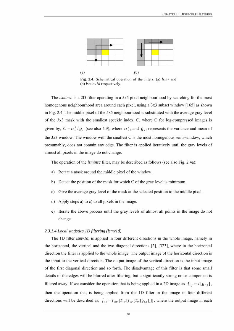
CHAPTER II: DESPECKLE FILTERING
(a) (b)
Fig. 2.4: Schematical operation of the filters: (a) lsmv and (b) lsminv1d respectively.
The lsminsc is a 2D filter operating in a 5x5 pixel neighbourhood by searching for the most
homogenous neighbourhood area around each pixel, using a 3x3 subset window [165] as shown
in Fig. 2.4. The middle pixel of the 5x5 neighbourhood is substituted with the average gray level
of the 3x3 mask with the smallest speckle index, C, where C for log-compressed images is
given by, ss gC /2σ= (see also 4.9), where , and 2sσ sg , represents the variance and mean of
the 3x3 window. The window with the smallest C is the most homogenous semi-window, which
presumably, does not contain any edge. The filter is applied iteratively until the gray levels of
almost all pixels in the image do not change.
The operation of the lsminsc filter, may be described as follows (see also Fig. 2.4a):
a) Rotate a mask around the middle pixel of the window.
b) Detect the position of the mask for which C of the gray level is minimum.
c) Give the average gray level of the mask at the selected position to the middle pixel.
d) Apply steps a) to c) to all pixels in the image.
e) Iterate the above process until the gray levels of almost all points in the image do not
change.
2.3.1.4 Local statistics 1D filtering (lsmv1d)
The 1D filter lsmv1d, is applied in four different directions in the whole image, namely in
the horizontal, the vertical and the two diagonal directions [2], [323], where in the horizontal
direction the filter is applied to the whole image. The output image of the horizontal direction is
the input to the vertical direction. The output image of the vertical direction is the input image
of the first diagonal direction and so forth. The disadvantage of this filter is that some small
details of the edges will be blurred after filtering, but a significantly strong noise component is
filtered away. If we consider the operation that is being applied in a 2D image as ][ ,, jiji gTf = ,
then the operation that is being applied from the 1D filter in the image in four different
directions will be described as, ]]]][[[[ ,09045135, jiji gTTTTf °°°°= , where the output image in each
38
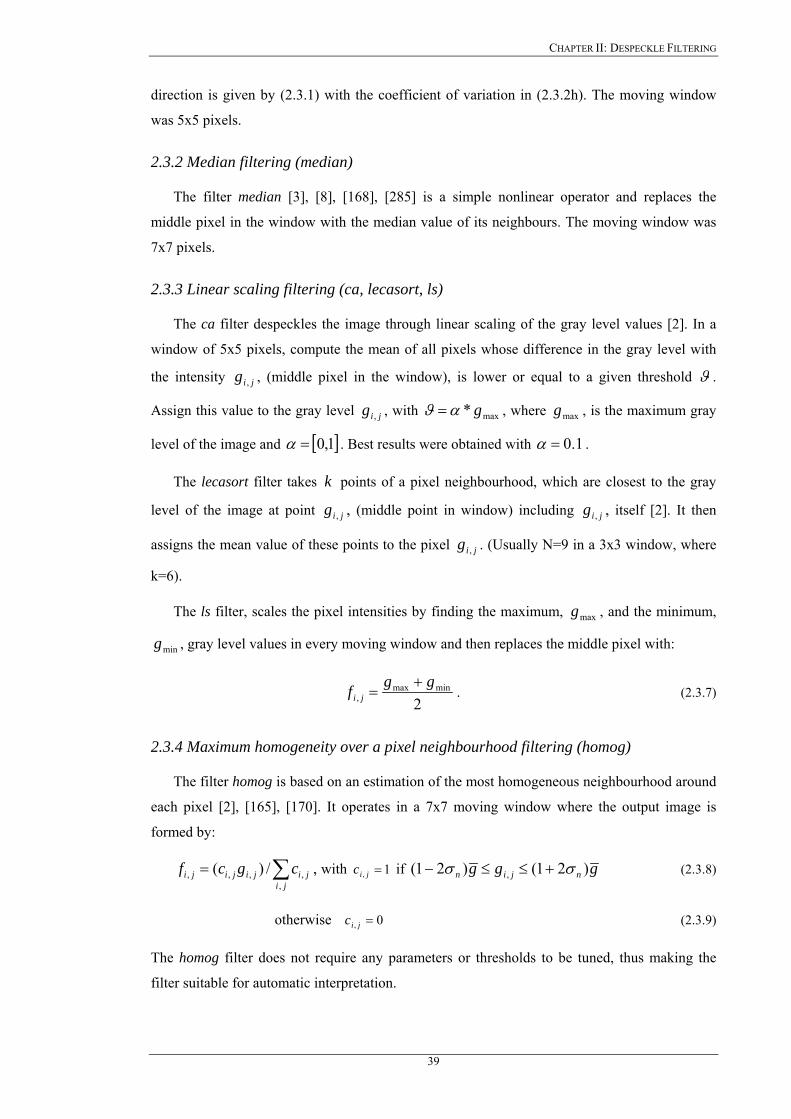
CHAPTER II: DESPECKLE FILTERING
direction is given by (2.3.1) with the coefficient of variation in (2.3.2h). The moving window
was 5x5 pixels.
2.3.2 Median filtering (median)
The filter median [3], [8], [168], [285] is a simple nonlinear operator and replaces the
middle pixel in the window with the median value of its neighbours. The moving window was
7x7 pixels.
2.3.3 Linear scaling filtering (ca, lecasort, ls)
The ca filter despeckles the image through linear scaling of the gray level values [2]. In a
window of 5x5 pixels, compute the mean of all pixels whose difference in the gray level with
the intensity , (middle pixel in the window), is lower or equal to a given threshold jig , ϑ .
Assign this value to the gray level , with jig , max* gαϑ = , where , is the maximum gray
level of the image and
maxg
[ 1,0= ]α . Best results were obtained with 1.0=α .
The lecasort filter takes k points of a pixel neighbourhood, which are closest to the gray
level of the image at point , (middle point in window) including , itself [2]. It then
assigns the mean value of these points to the pixel . (Usually N=9 in a 3x3 window, where
k=6).
jig , jig ,
jig ,
The ls filter, scales the pixel intensities by finding the maximum, , and the minimum,
, gray level values in every moving window and then replaces the middle pixel with:
maxg
ming
2
minmax,
ggf ji+
= . (2.3.7)
2.3.4 Maximum homogeneity over a pixel neighbourhood filtering (homog)
The filter homog is based on an estimation of the most homogeneous neighbourhood around
each pixel [2], [165], [170]. It operates in a 7x7 moving window where the output image is
formed by:
∑=ji
jijijiji cgcf,
,,,, /)( , with 1, =jic if ggg njin )21()21( , σσ +≤≤− (2.3.8)
otherwise 0, =jic (2.3.9)
The homog filter does not require any parameters or thresholds to be tuned, thus making the
filter suitable for automatic interpretation.
39
CHAPTER II: DESPECKLE FILTERING
2.3.5 Geometric filtering (gf4d, gfminmax)
The geometric despeckle filter gf4d, works by passing an image through a speckle-removing
filter, which uses the complementary hulling technique [19], [162], (raising pixels that are
darker than their surrounding neighbours, then complementarily lowering pixels that are
brighter than their surrounding neighbours) to reduce the speckle index, C, of that image. The
filter uses a non-linear noise reduction technique, which compares the intensity of each pixel in
an image with those of its 8 nearest neighbours (3x3 neighbourhood) and, based upon the
relative values, increments or decrements the value of the pixel in question such that it becomes
more representative of its surroundings. The filtering process involves a series of pair wise
operations in which the value of the middle pixel within each neighbourhood window is
compared, in turn, with each set of neighbours (N-ST, E-W, NW-STE, NE-STW, see Fig. 2.5)
in a search for intensity spikes.
Suppose that the three consecutive pixels (e.g. on a N-ST column) that are being examined
are a, b, c (see Fig. 2.5). The operation of the geometric filter gf4d may be described with Fig.
2.5 and has the following form:
a) Select direction and assign pixel values. Select the direction be NST and the
corresponding three consecutive pixels be a, b, c (see Fig. 2.5a and b).
b) Carry out central pixel adjustments. Do the following intensity adjustments (see Fig.
2.5b)
if 2+≥ ba then 1+= bb ,
if and ba f cb ≤ then 1+= bb ,
if and bc f ab ≤ then 1+= bb , (2.3.10)
if 2+≥ bc then 1+= bb ,
if 2−≤ ba then 1−= bb ,
if and then ba p cb ≥ 1−= bb ,
if and then bc p ab ≥ 1−= bb ,
if 2−≤ bc then 1−= bb .
c) Repeat steps 1 and 2 for west-east (WE), west-north to south-east (WN-STE), and
north-east to west-south (NE-WST) directions.
40
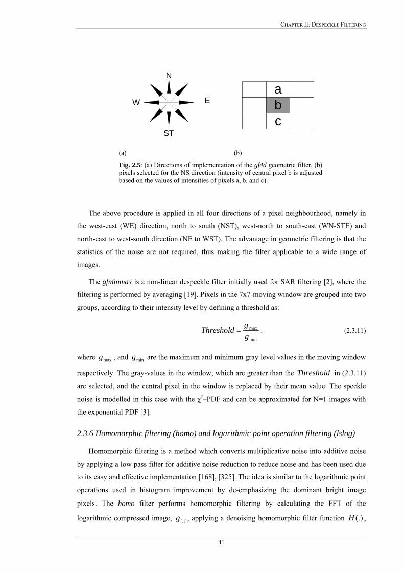
CHAPTER II: DESPECKLE FILTERING
EW
N
ST
abc
(a) (b)
Fig. 2.5: (a) Directions of implementation of the gf4d geometric filter, (b) pixels selected for the NS direction (intensity of central pixel b is adjusted based on the values of intensities of pixels a, b, and c).
The above procedure is applied in all four directions of a pixel neighbourhood, namely in
the west-east (WE) direction, north to south (NST), west-north to south-east (WN-STE) and
north-east to west-south direction (NE to WST). The advantage in geometric filtering is that the
statistics of the noise are not required, thus making the filter applicable to a wide range of
images.
The gfminmax is a non-linear despeckle filter initially used for SAR filtering [2], where the
filtering is performed by averaging [19]. Pixels in the 7x7-moving window are grouped into two
groups, according to their intensity level by defining a threshold as:
min
max
ggThreshold = . (2.3.11)
where , and are the maximum and minimum gray level values in the moving window
respectively. The gray-values in the window, which are greater than the in (2.3.11)
are selected, and the central pixel in the window is replaced by their mean value. The speckle
noise is modelled in this case with the χ
maxg ming
Threshold
2–PDF and can be approximated for N=1 images with
the exponential PDF [3].
2.3.6 Homomorphic filtering (homo) and logarithmic point operation filtering (lslog)
Homomorphic filtering is a method which converts multiplicative noise into additive noise
by applying a low pass filter for additive noise reduction to reduce noise and has been used due
to its easy and effective implementation [168], [325]. The idea is similar to the logarithmic point
operations used in histogram improvement by de-emphasizing the dominant bright image
pixels. The homo filter performs homomorphic filtering by calculating the FFT of the
logarithmic compressed image, , applying a denoising homomorphic filter function , jig , (.)H
41
CHAPTER II: DESPECKLE FILTERING
and then performing the inverse FFT of the image [229] to form the despeckled image . The
homomorphic filter function maybe constructed either using a band-pass Butterworth or a
high-boost Butterworth filter. In this study, a high-boost Butterworth filter was used for the
homomorphic function with [229]:
jif ,
(.)H
(.)H
20 )),(/(1
),(vuDD
vuH HL ++=
γγ (2.3.12)
and 22 )2/()2/(),( NvNuvuD −+−= (2.3.13)
where is the cut of frequency of the filter, 8.10 =D 4.0=Lγ , 6.0=Hγ are the gains for the
low and high frequencies, u , are the spatial coordinates of the frequency transformed image,
and N the dimensions of the image in the , , space respectively.
vu v
The homomorphic filtering is effective mainly on images with relatively low contrast [122],
and there are researchers [196] that reported undesirable artefacts on MRI with this approach.
The lslog filter [324], assumes a multiplicative white noise model and transforms the
multiplicative to additive noise by using the logarithm of the image. At the beginning, the
logarithm of the noise image is calculated, the median filter for additive noise [285] is then
applied on the image, and the resulting image is transformed exponentially back to its initial
form. This type of filtering refers to a technique [37], [123] of pre-processing the observed
image by transforming multiplicative noise into additive noise form, using some linear memory
less operator.
2.3.7 Diffusion filtering
Diffusion filters remove noise from an image by modifying the image via solving a partial
differential equation (PDE). Despeckling is carried out depending on the image edges and their
directions. Anisotropic diffusion is an efficient nonlinear technique for simultaneously
performing contrast enhancement and noise reduction [37], [38], [324], [326], [344]-[347],
without requiring any information from the image power spectrum. It may thus directly be
applied to logarithmic compressed images. Consider applying the isotropic diffusion equation
given by )(/,, gcddivdtdg tji ∇= , using the original noisy image , as the initial
condition, where , is an image in the continuous domain,
0,, =tjig
0,, =tjig ji, , specifies spatial position,
is an artificial time parameter, , is the diffusion constant, and t cd g∇ , is the image gradient.
In the next Sections we present anisotropic diffusion (ad), speckle anisotropic diffusion
(adsr), and coherent nonlinear anisotropic diffusion (nldif). Anisotropic diffusion filters usually
require many iteration steps compared with the local statistic filters.
42
CHAPTER II: DESPECKLE FILTERING
2.3.7.1 Anisotropic diffusion filtering (ad)
Perona and Malik [347] replaced the classical isotropic diffusion equation, as described
above, by the introduction of a function, )(,, gfcd tji ∇= , with:
[ ] ⎥⎦
⎤⎢⎣
⎡+⎥⎦
⎤⎢⎣⎡=∇= tjitjitjitjitjitji
tji gdjdcd
djdg
didcd
didgcddiv
dtdg
,,,,,,,,,,,,,, (2.3.14)
where g∇ , is the gradient magnitude, and )( gcd ∇ , is an edge stopping function, which is
chosen to satisfy , when 0→cd ∞→∇g , so that the diffusion is stopped across edges. This
function, called the diffusion coefficient, )( gcd ∇ , which is a monotonically decreasing
function of the gradient magnitude, g∇ , yields intra-region smoothing not inter-region
smoothing [167], [326], [344], [346], [347], by stopping diffusion at the image edges. It
increases smoothing parallel to the edge and stops smoothing perpendicular to the edge, as the
highest gradient values are perpendicular to the edge and dilated across edges. In anisotropic
diffusion the diffusion coefficient is allowed to vary according to the local image gradient. The
choice of )( gcd ∇ , can greatly affect the extent to which discontinuities are preserved. For
example if, )( gcd ∇ , is constant at all locations, then smoothing progresses in an isotropic
manner. If )( gcd ∇ , is allowed to vary according to the local image gradient, then we have
anisotropic diffusion. A basic anisotropic PDE is given in (2.3.14). Two different diffusion
coefficients were proposed in [347] and derived in [346] as follows:
2, )/(1
1)(Kg
gcdji∇+
=∇ , (2.3.15)
and 21,
,
)/(22
)(Kg
ggcd
ji
ji
∇+
∇=∇ (2.3.16)
where K in (2.3.15) is a positive gradient threshold parameter, known as diffusion or flow
constant, and for (2.3.16) [326], [346]. In this study the diffusion coefficient in
(2.3.15) was used, which was found to perform better in the carotid artery ultrasound images.
2/221 KK =
A discrete formulation of the anisotropic diffusion in (2.3.14) is given by [38], [326], [346],
[347]:
[ ] [ ] [ ] [{ },,1,,1,,1,,1,,,1,,1,,1,,1,
jijitjijijitjijijitjijijitjis
dji ggcdggcdggcdggcddt
dg−+−+−+−= −−++−−++η
λ ] (2.3.17 a)
where the new pixel gray value, , at location jif , ji, is:
43
CHAPTER II: DESPECKLE FILTERING
,41 ,
,, dtdg
gf jijiji += (2.3.17 b)
where , , , and , are the diffusion coefficients for the west, east,
north and south pixel directions, in a four pixel neighborhood, around the pixel
tjicd ,,1+ tjicd ,,1− tjicd ,1, + tjicd ,1, −
ji, , where
diffusion is computed respectively. The coefficient of variation leads to the largest diffusion
where the nearest-neighbor difference is largest (strongest edge), while the smallest diffusion is
calculated where the nearest-neighbor difference is smallest (the weakest edge). The constant
is a scalar that determines the rate of diffusion, +ℜ∈dλ sη represents the spatial neighborhood
of pixel ji, , and sη is the number of neighbors (usually four except at the image boundaries).
Perona and Malik [347] linearly approximated the directional derivative in a particular direction
as (for the west neighbor of the central pixel jijiji ggg ,,1, −=∇ + ji, ). Modifying the image
according to the above equation in (2.3.17), which is a linear isotropic diffusion equation, is
equivalent to filtering the image with a Gaussian filter. The parameters for the anisotropic
diffusion filter used in this study were, 25.0=dλ , 8=sη , and the parameter , which
was used for the calculation of the diffusion coefficient
30=K
)( gcd ∇ in (2.3.15).
2.3.7.2 Lee diffusion and speckle reducing anisotropic diffusion filtering (lsmedcd, adsr)
By assigning slightly different weights to (2.3.17), the output of the filter lsmedcd, may be
formed as [38]:
)1(1,,,, jiji
sjiji gkdivgf ∇−+=
η (2.3.18)
with the weighting factor, , which can be calculated with (2.3.2a)-(2.3.2h). The lsmedcd
filter as shown in (2.3.18) operates in 8 different directions within the moving window.
jik ,
The essence of speckle reducing anisotropic diffusion is the replacement of the gradient
based edge detector, )( gcd ∇ , in original anisotropic diffusion PDE with the instantaneous
coefficient of variation suitable for speckle filtering, )( gcadsr ∇ . The adsr speckle reducing
anisotropic diffusion filter [38], uses two seemingly different methods, namely the Lee [22]-
[26], [159] and the Frost diffusion filters [27], [28]. A more general updated function for the
output image by extending the PDE versions of the despeckle filter is [38], [74]:
))((1,,, jiadsr
sjiji ggcdivgf ∇∇+=
η. (2.3.19)
The diffusion coefficient for the speckle anisotropic diffusion, )( gcadsr ∇ , is derived [38] as:
44
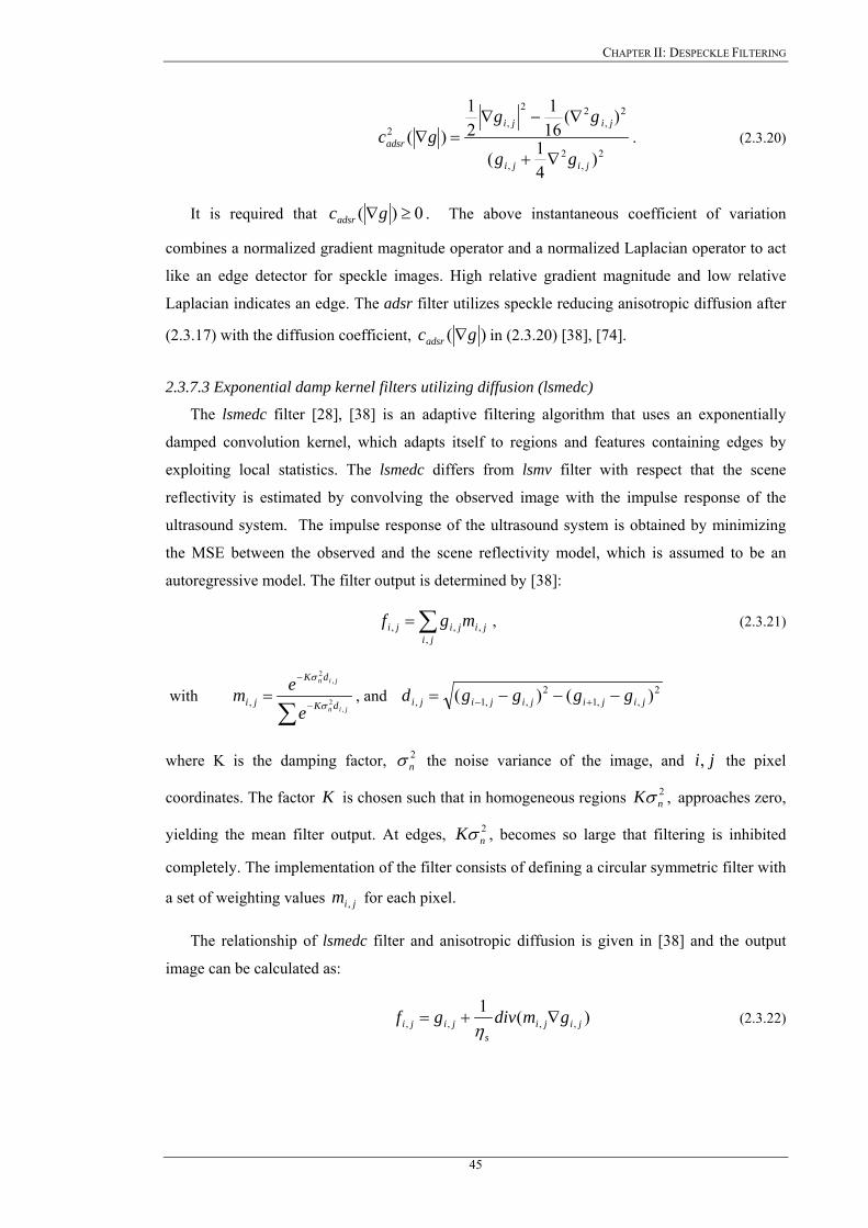
CHAPTER II: DESPECKLE FILTERING
2
,2
,
2,
22
,2
)41(
)(161
21
)(jiji
jiji
adsr
gg
gggc
∇+
∇−∇=∇ . (2.3.20)
It is required that 0)( ≥∇gcadsr . The above instantaneous coefficient of variation
combines a normalized gradient magnitude operator and a normalized Laplacian operator to act
like an edge detector for speckle images. High relative gradient magnitude and low relative
Laplacian indicates an edge. The adsr filter utilizes speckle reducing anisotropic diffusion after
(2.3.17) with the diffusion coefficient, )( gcadsr ∇ in (2.3.20) [38], [74].
2.3.7.3 Exponential damp kernel filters utilizing diffusion (lsmedc)
The lsmedc filter [28], [38] is an adaptive filtering algorithm that uses an exponentially
damped convolution kernel, which adapts itself to regions and features containing edges by
exploiting local statistics. The lsmedc differs from lsmv filter with respect that the scene
reflectivity is estimated by convolving the observed image with the impulse response of the
ultrasound system. The impulse response of the ultrasound system is obtained by minimizing
the MSE between the observed and the scene reflectivity model, which is assumed to be an
autoregressive model. The filter output is determined by [38]:
∑=ji
jijiji mgf,
,,, , (2.3.21)
with ∑ −
−
=jin
jin
dK
dK
jie
em,
2
,2
, σ
σ
, and 2,,1
2,,1, )()( jijijijiji ggggd −−−= +−
where K is the damping factor, the noise variance of the image, and 2nσ ji, the pixel
coordinates. The factor K is chosen such that in homogeneous regions , 2nKσ approaches zero,
yielding the mean filter output. At edges, , becomes so large that filtering is inhibited
completely. The implementation of the filter consists of defining a circular symmetric filter with
a set of weighting values for each pixel.
2nKσ
jim ,
The relationship of lsmedc filter and anisotropic diffusion is given in [38] and the output
image can be calculated as:
)(1,,,, jiji
sjiji gmdivgf ∇+=
η (2.3.22)
45
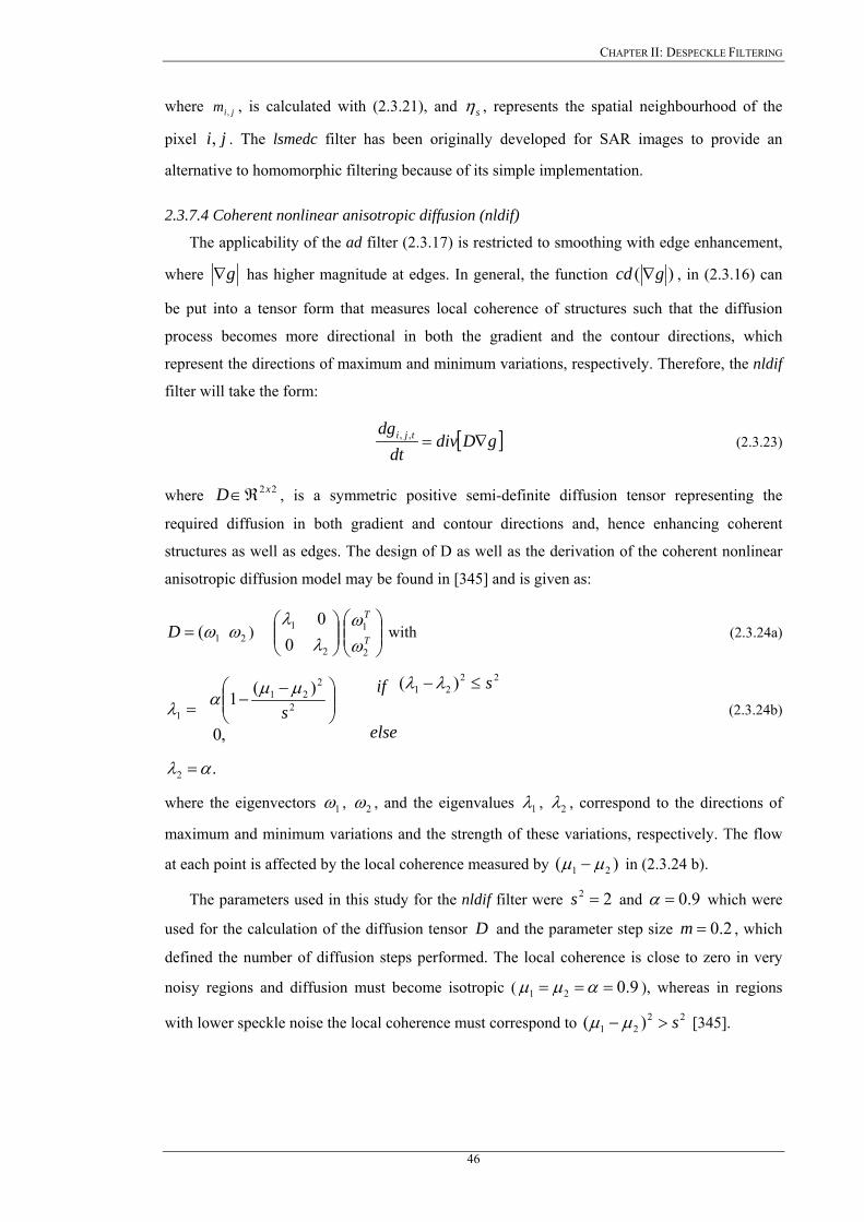
CHAPTER II: DESPECKLE FILTERING
where , is calculated with (2.3.21), and jim , sη , represents the spatial neighbourhood of the
pixel ji, . The lsmedc filter has been originally developed for SAR images to provide an
alternative to homomorphic filtering because of its simple implementation.
2.3.7.4 Coherent nonlinear anisotropic diffusion (nldif)
The applicability of the ad filter (2.3.17) is restricted to smoothing with edge enhancement,
where g∇ has higher magnitude at edges. In general, the function )( gcd ∇ , in (2.3.16) can
be put into a tensor form that measures local coherence of structures such that the diffusion
process becomes more directional in both the gradient and the contour directions, which
represent the directions of maximum and minimum variations, respectively. Therefore, the nldif
filter will take the form:
[ ]gDdivdt
dg tji ∇=,, (2.3.23)
where , is a symmetric positive semi-definite diffusion tensor representing the
required diffusion in both gradient and contour directions and, hence enhancing coherent
structures as well as edges. The design of D as well as the derivation of the coherent nonlinear
anisotropic diffusion model may be found in [345] and is given as:
22xD ℜ∈
1(ω=D 2ω ) with (2.3.24a) ⎟⎟⎠
⎞⎜⎜⎝
⎛
2
1
00λ
λ⎟⎟⎠
⎞⎜⎜⎝
⎛T
T
2
1
ωω
2221
2
221
1
)(
,0
)(1s
else
ifs
≤−⎟⎟⎠
⎞⎜⎜⎝
⎛ −−=
λλµµαλ (2.3.24b)
.2 αλ =
where the eigenvectors 1ω , 2ω , and the eigenvalues 1λ , 2λ , correspond to the directions of
maximum and minimum variations and the strength of these variations, respectively. The flow
at each point is affected by the local coherence measured by )( 21 µµ − in (2.3.24 b).
The parameters used in this study for the nldif filter were and 22 =s 9.0=α which were
used for the calculation of the diffusion tensor and the parameter step size , which
defined the number of diffusion steps performed. The local coherence is close to zero in very
noisy regions and diffusion must become isotropic (
D 2.0=m
9.021 === αµµ ), whereas in regions
with lower speckle noise the local coherence must correspond to [345]. 2221 )( s>− µµ
46
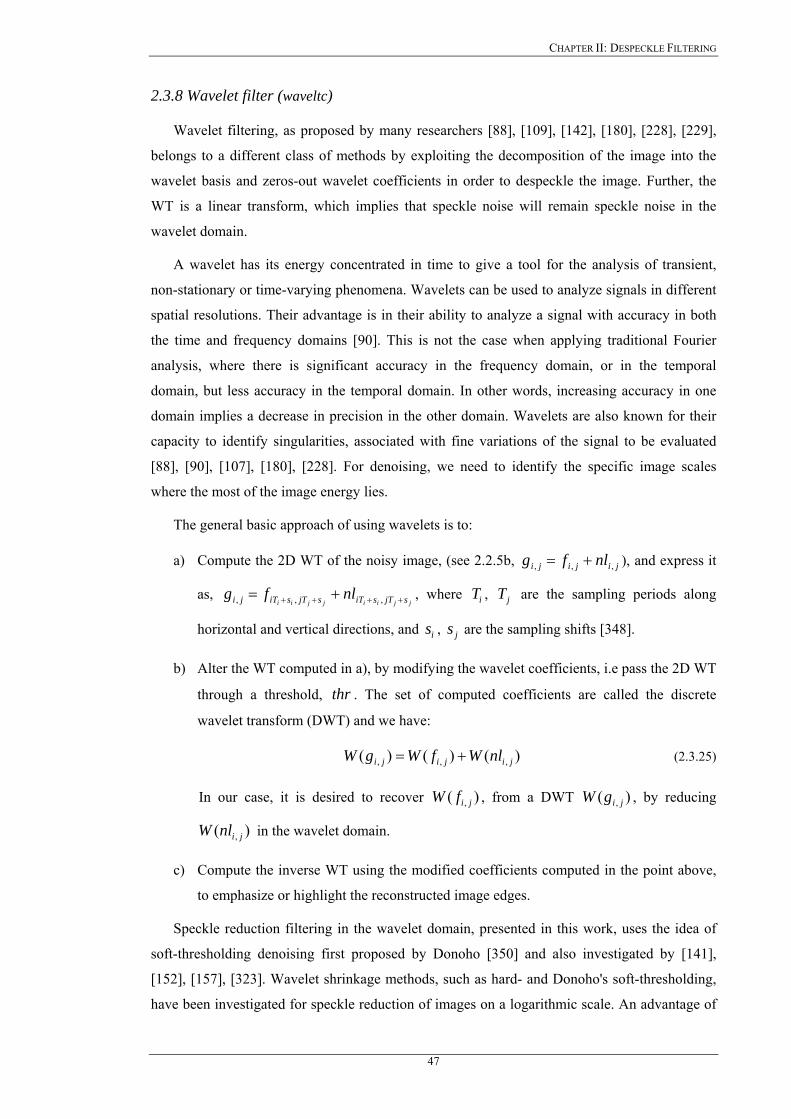
CHAPTER II: DESPECKLE FILTERING
2.3.8 Wavelet filter (waveltc)
Wavelet filtering, as proposed by many researchers [88], [109], [142], [180], [228], [229],
belongs to a different class of methods by exploiting the decomposition of the image into the
wavelet basis and zeros-out wavelet coefficients in order to despeckle the image. Further, the
WT is a linear transform, which implies that speckle noise will remain speckle noise in the
wavelet domain.
A wavelet has its energy concentrated in time to give a tool for the analysis of transient,
non-stationary or time-varying phenomena. Wavelets can be used to analyze signals in different
spatial resolutions. Their advantage is in their ability to analyze a signal with accuracy in both
the time and frequency domains [90]. This is not the case when applying traditional Fourier
analysis, where there is significant accuracy in the frequency domain, or in the temporal
domain, but less accuracy in the temporal domain. In other words, increasing accuracy in one
domain implies a decrease in precision in the other domain. Wavelets are also known for their
capacity to identify singularities, associated with fine variations of the signal to be evaluated
[88], [90], [107], [180], [228]. For denoising, we need to identify the specific image scales
where the most of the image energy lies.
The general basic approach of using wavelets is to:
a) Compute the 2D WT of the noisy image, (see 2.2.5b, jijiji nlfg ,,, += ), and express it
as, jjiijjii sjTsiTsjTsiTji nlfg ++++ += ,,, , where , are the sampling periods along
horizontal and vertical directions, and , are the sampling shifts [348].
iT jT
is js
b) Alter the WT computed in a), by modifying the wavelet coefficients, i.e pass the 2D WT
through a threshold, thr . The set of computed coefficients are called the discrete
wavelet transform (DWT) and we have:
)()()( ,,, jijiji nlWfWgW += (2.3.25)
In our case, it is desired to recover , from a DWT , by reducing
in the wavelet domain.
)( , jifW )( , jigW
)( , jinlW
c) Compute the inverse WT using the modified coefficients computed in the point above,
to emphasize or highlight the reconstructed image edges.
Speckle reduction filtering in the wavelet domain, presented in this work, uses the idea of
soft-thresholding denoising first proposed by Donoho [350] and also investigated by [141],
[152], [157], [323]. Wavelet shrinkage methods, such as hard- and Donoho's soft-thresholding,
have been investigated for speckle reduction of images on a logarithmic scale. An advantage of
47
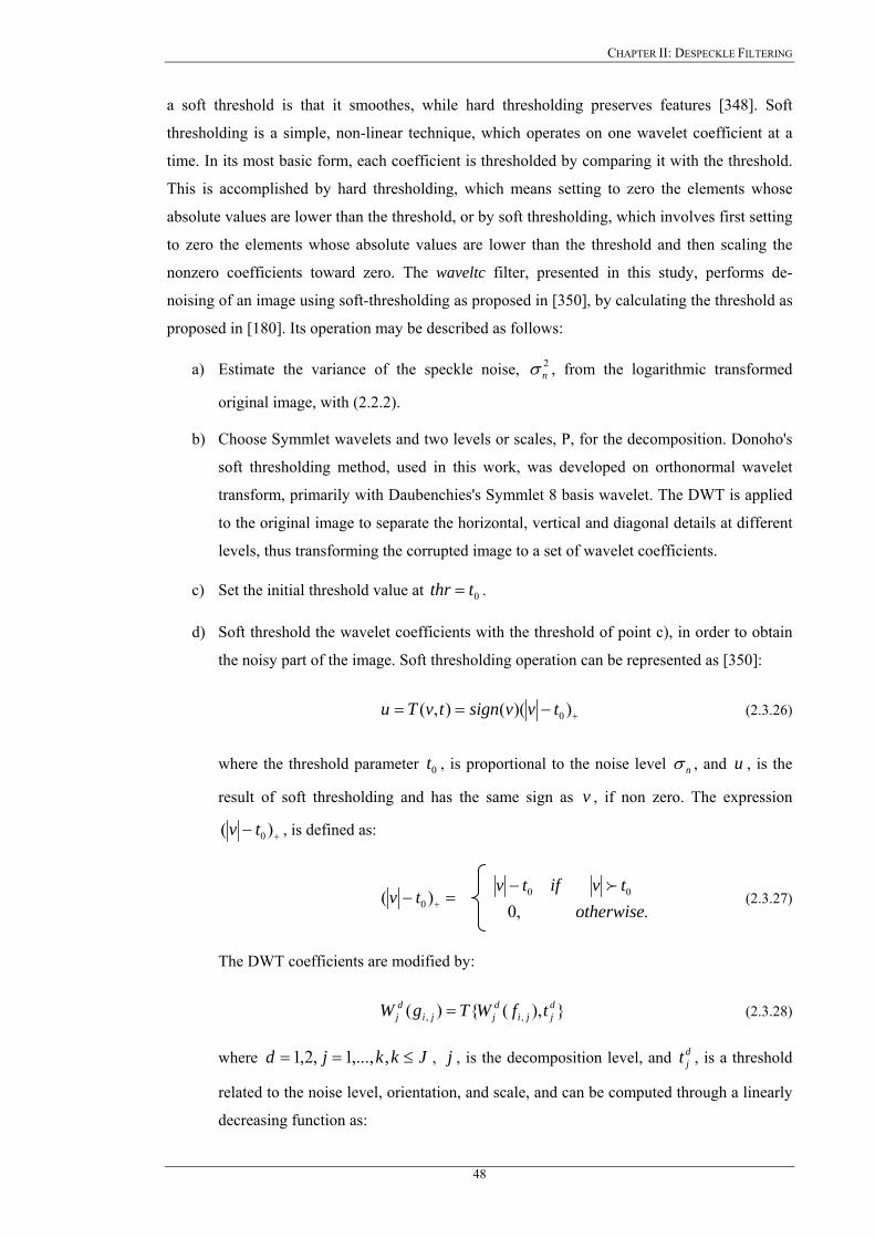
CHAPTER II: DESPECKLE FILTERING
a soft threshold is that it smoothes, while hard thresholding preserves features [348]. Soft
thresholding is a simple, non-linear technique, which operates on one wavelet coefficient at a
time. In its most basic form, each coefficient is thresholded by comparing it with the threshold.
This is accomplished by hard thresholding, which means setting to zero the elements whose
absolute values are lower than the threshold, or by soft thresholding, which involves first setting
to zero the elements whose absolute values are lower than the threshold and then scaling the
nonzero coefficients toward zero. The waveltc filter, presented in this study, performs de-
noising of an image using soft-thresholding as proposed in [350], by calculating the threshold as
proposed in [180]. Its operation may be described as follows:
a) Estimate the variance of the speckle noise, , from the logarithmic transformed
original image, with (2.2.2).
2nσ
b) Choose Symmlet wavelets and two levels or scales, P, for the decomposition. Donoho's
soft thresholding method, used in this work, was developed on orthonormal wavelet
transform, primarily with Daubenchies's Symmlet 8 basis wavelet. The DWT is applied
to the original image to separate the horizontal, vertical and diagonal details at different
levels, thus transforming the corrupted image to a set of wavelet coefficients.
c) Set the initial threshold value at 0tthr = .
d) Soft threshold the wavelet coefficients with the threshold of point c), in order to obtain
the noisy part of the image. Soft thresholding operation can be represented as [350]:
+−== ))((),( 0tvvsigntvTu (2.3.26)
where the threshold parameter , is proportional to the noise level 0t nσ , and , is the
result of soft thresholding and has the same sign as , if non zero. The expression
u
v
+− )( 0tv , is defined as:
.,0
)( 000 otherwise
tviftvtv
f−=− + (2.3.27)
The DWT coefficients are modified by:
(2.3.28) }),({)( ,,djji
djji
dj tfWTgW =
where Jkkjd ≤== ,,...,1,2,1 , j , is the decomposition level, and , is a threshold
related to the noise level, orientation, and scale, and can be computed through a linearly
decreasing function as:
djt
48

CHAPTER II: DESPECKLE FILTERING
otherwiseTTjTifjT
t dj
djd
j ,)1())1((
min
minmaxmax
σασα f−−−−
= (2.3.29)
where , is the standard deviation, djσ α , is a decreasing factor between two consecutive
levels, , , are a maximum and a minimum factor for , with, maxT minT djσ Jj ≤≤1 , and
. For the case of an unknown noise level, we use , to estimate the noise
level of the image. The threshold , is primarily calculated using, , and a
decreasing factor,
}2,1{∈d djσ
djt d
jσ
)1(max −− jT α . Donoho [350] proposed a threshold for additive
noise such as, )log(2 Nthr nσ= , [90], [350], where nσ , is the noise standard
deviation in the image, and N is the block size in the wavelet transform (i.e N=8). Hard
threshold rule usually leads to small MSE where soft-threshold can maintain the
smoothness of the original signal. The threshold is estimated by using denoising
decomposition at two levels with symmetry wavelets [90], [350].
e) Perform the inverse WT.
f) Calculate the standard deviation of the noisy image.
g) Calculate the difference between the estimated deviation and the calculated deviation. If
the difference is below the tolerance in step c), then got to i).
h) Renew the threshold deltathresholdofstepthrthr *__+= . Go to d).
i) Subtract the noisy image from the original image to obtain the despeckled image.
49

CHAPTER III: IMT AND PLAQUE SEGMENTATION
Chapter 3
IMT And Plaque Segmentation
50
CHAPTER III: IMT AND PLAQUE SEGMENTATION
CHAPTER 3: IMT AND PLAQUE SEGMENTATION
Outlining or segmenting organs and specifically the carotid artery or plaque is an important
task in the treatment of the subject under investigation. However, manual outlining is tedious,
time consuming and suffers from intra- and inter-observer variability. New techniques are
therefore needed for accomplishing the above tasks.
In this Chapter an introduction to previous work on IMT and plaque segmentation on
ultrasound imaging is addressed, and deformable models are briefly introduced. Furthermore,
the theoretical concepts of the IMT and plaque snakes segmentation method in 2D ultrasound
images of the carotid artery are explained. The IMT snakes segmentation method, utilizes
normalization, despeckling, and an automatic contour initialization, for initially positioning the
snake, which is then deformed to accurately fit the desired boundaries. The plaque snakes
segmentation method uses the blood flow image first to detect the initial contour of the plaque,
and then despeckle filtering and snakes to deform the initial contour for best fit of plaque
boundaries. Finally, reference is given to some other snake methods, and the snake initialisation
procedures for the IMT and plaque are presented.
3.1 Introduction
The aim of image segmentation is to partition an image into a number of non-overlapping
regions that form a complete description of the image. A wide range of work has been
undertaken to achieve this aim and segmentation has found diverse applications ranging from
medical to military. It is still a subject of an on-going investigation and it cannot be conclusively
stated that the segmentation problem has been solved. For the goal of delineating the IMT, and
the plaque borders in the carotid artery, it is not necessary to obtain a complete segmentation of
the image, but to obtain a partial segmentation so that discriminates between wall and blood and
wall and plaque borders.
In this Chapter, we focus on the IMT and plaque segmentation from ultrasound images of
the carotid artery by utilising despeckle filtering as explained in Chapter 2. The relation of
despeckle filtering and segmentation may be explained as follows. Despeckling may be used as
a pre-processing step for the segmentation. Most existing segmentation techniques like active
contours and the watershed transform (WT), process gradient information in the image. Because
of the relatively low SNR in ultrasound images, speckle noise degrades the performance of
these techniques considerably [220], [238], [335], [338], so that active contours, and other
segmentation techniques might get stuck in the speckle noise. By despeckle filtering the
performance of the segmentation techniques might be enhanced.
51
CHAPTER III: IMT AND PLAQUE SEGMENTATION
Extracting the boundaries of objects in images is one of the most important problems in
computer vision and image processing. A wide variety of mathematical and computational
approaches have been proposed for solving segmentation problems. Surveys of segmentation
methods concerning the most common algorithms have been undertaken by Haralick et al.
[128], and most image processing texts generally provide a broad overview of the more
common algorithms [1]-[9], [111].
Several other techniques have also been proposed in the literature to segment the cavities of
the heart in ultrasound images [175], [190], [218] tumours in the liver [211], [354], and the
prostate [80]. Furthermore, several classical segmentation techniques have been described under
which, the most recent is the HT [150], [151], [201], [204], the WT [11], [135], [137], [140],
[143], and active contours, or snakes [242]-[256]. Some more traditional segmentation
techniques include, histogram analysis [211], region growing and spit-merge algorithms [3],
[245], colour space analysis and segmentation [7]-[9], pixel classification for segmentation [3]-
[9], gradient segmentation [148], [251], [258], edge and zero-crossing detectors such as Canny
[128], and radial search and boundary following algorithms [7]-[9]. Instead of exploiting only
pixel information as low-level edge-detection techniques do, active contours or snakes [243],
also use information about the boundaries as part of an optimization procedure. Active contours
are used extensively for segmentation, and a number of alternative approaches have been
proposed such as, geometric deformable models, [60], [225], discrete dynamic contour [222],
geometric active contours, [60], [95], [179], [225] and level sets [97], [111], [179], [221], [239].
When the exact shape of an object is unknown or is impossible to parameterize it, techniques
that can evolve the target solution or adapt their result to the image are used. This implies the
use of flexible shape formulations [155]. Another disadvantage of these methods is that
spectrally similar but spatially disjoint regions are never associated together, thus complicating
their identification. Also, it is often not clear at what point the region growing process should be
terminated, resulting in under- and over-segmentation. In addition the region growing approach
tends to be a very computationally intensive process. As it is shown in the literature, snakes get
stuck because of the strong speckle noise [231], the HT [201], [218], and the WT [11] shows
over or under segmentation. Furthermore, the HT and the WT methods are slow and pose
problems with the initial contour initialisation [204].
In the next section we present previous work on carotid IMT and plaque segmentation. Also
we introduce theoretical concepts on snakes, and explain why snakes have been chosen to
segment the IMT and plaque from ultrasound images of the carotid artery.
52
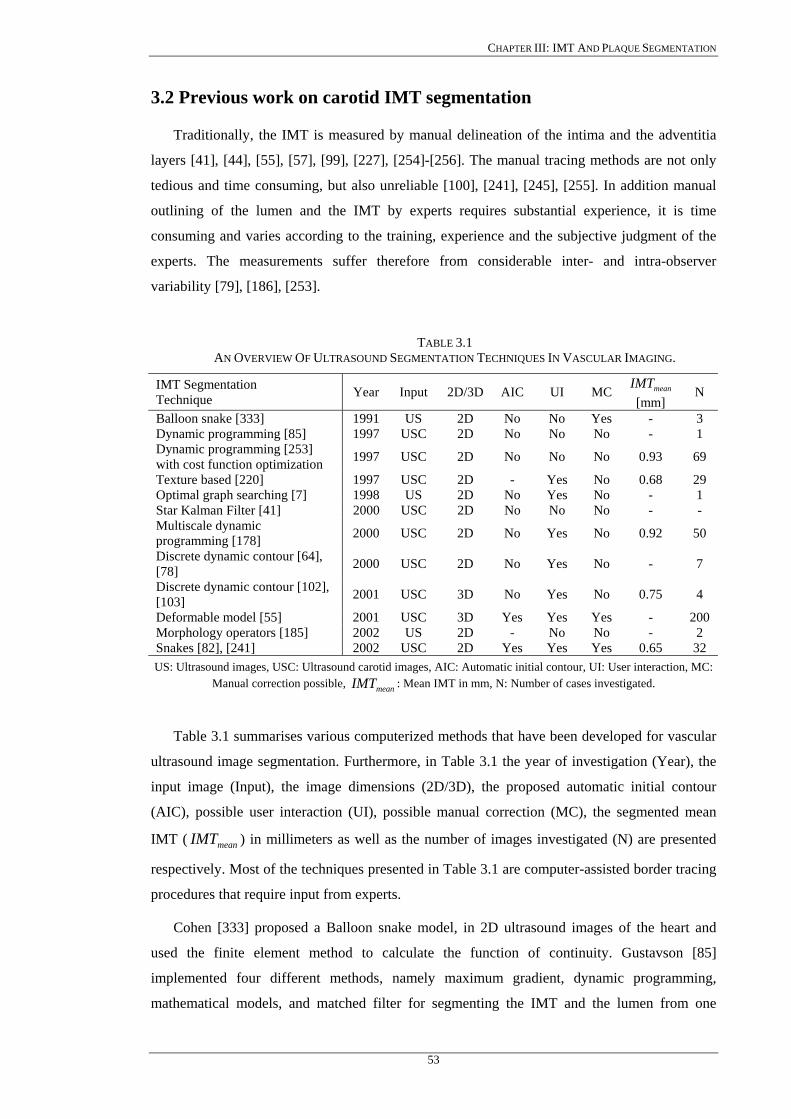
CHAPTER III: IMT AND PLAQUE SEGMENTATION
3.2 Previous work on carotid IMT segmentation
Traditionally, the IMT is measured by manual delineation of the intima and the adventitia
layers [41], [44], [55], [57], [99], [227], [254]-[256]. The manual tracing methods are not only
tedious and time consuming, but also unreliable [100], [241], [245], [255]. In addition manual
outlining of the lumen and the IMT by experts requires substantial experience, it is time
consuming and varies according to the training, experience and the subjective judgment of the
experts. The measurements suffer therefore from considerable inter- and intra-observer
variability [79], [186], [253].
TABLE 3.1 AN OVERVIEW OF ULTRASOUND SEGMENTATION TECHNIQUES IN VASCULAR IMAGING.
IMT Segmentation Technique Year Input 2D/3D AIC UI MC meanIMT
[mm] N
Balloon snake [333] 1991 US 2D No No Yes - 3 Dynamic programming [85] 1997 USC 2D No No No - 1 Dynamic programming [253] with cost function optimization 1997 USC 2D No No No 0.93 69
Texture based [220] 1997 USC 2D - Yes No 0.68 29 Optimal graph searching [7] 1998 US 2D No Yes No - 1 Star Kalman Filter [41] 2000 USC 2D No No No - - Multiscale dynamic programming [178] 2000 USC 2D No Yes No 0.92 50
Discrete dynamic contour [64], [78] 2000 USC 2D No Yes No - 7
Discrete dynamic contour [102], [103] 2001 USC 3D No Yes No 0.75 4
Deformable model [55] 2001 USC 3D Yes Yes Yes - 200 Morphology operators [185] 2002 US 2D - No No - 2 Snakes [82], [241] 2002 USC 2D Yes Yes Yes 0.65 32 US: Ultrasound images, USC: Ultrasound carotid images, AIC: Automatic initial contour, UI: User interaction, MC:
Manual correction possible, : Mean IMT in mm, N: Number of cases investigated. meanIMT
Table 3.1 summarises various computerized methods that have been developed for vascular
ultrasound image segmentation. Furthermore, in Table 3.1 the year of investigation (Year), the
input image (Input), the image dimensions (2D/3D), the proposed automatic initial contour
(AIC), possible user interaction (UI), possible manual correction (MC), the segmented mean
IMT ( ) in millimeters as well as the number of images investigated (N) are presented
respectively. Most of the techniques presented in Table 3.1 are computer-assisted border tracing
procedures that require input from experts.
meanIMT
Cohen [333] proposed a Balloon snake model, in 2D ultrasound images of the heart and
used the finite element method to calculate the function of continuity. Gustavson [85]
implemented four different methods, namely maximum gradient, dynamic programming,
mathematical models, and matched filter for segmenting the IMT and the lumen from one
53
CHAPTER III: IMT AND PLAQUE SEGMENTATION
longitudinal image of the carotid artery. The results showed that the dynamic programming
algorithm performed better than the others in respect of speed and boundary continuity,
although the detected boundaries could not be drawn correctly. Wendelhag et al. [253]
developed a computerized analysis system to extract the boundaries of the IMT using dynamic
programming with cost function optimization in longitudinal 2D images of the carotid artery.
However, the system requires manual correction after automatic tracing, and three weighting
factors must be tuned due to the varied characteristics of the ultrasound instrumentation.
In another study, Mojsilovic et al. [220] proposed a method for intra-vascular images of the
carotid artery based on textural operators to separate different tissue regions and morphological
processing to refine the extracted contours. Sonka et al. [7] proposed optimal graph searching
for ultrasound images of the carotid artery, but the algorithm requires manual and empirical
estimations to be made by the expert. Abolmaesumi [41] proposed a star algorithm to estimate
the center of the artery in transversal carotid images and a Kalman filter approach to estimate
the carotid artery boundary. The star algorithm was able to detect the center of the carotid by
considering it as the center of gravity but the results were not very accurate.
Liang et al. [178] applied multiscale dynamic programming to detect the approximate
boundaries of the carotid vessel walls in transversal 2D carotid artery images by reducing the
inter-observer variability. A cost function was proposed, which is a weighted sum of terms, in
fuzzy expression forms, representing image features and geometrical characteristics of the
vessel interfaces. This cost function was then used to guide the detection of the boundaries in a
fine scale image. The weights were adjusted by a training procedure, which was long and
required human experts tracing. Therefore, this method is not appropriate to evaluate a large
database of images, as strong human expert tracing and involvement is required.
In his research, Mao et al. [64], [78], proposed a deformable discrete dynamic contour
model in 2D transversal images of the carotid artery, with only one seed point to guide the
initialization of the deformable model for each lumen cross section. The snake initial contour
was generated using the entropy map of the image and morphological operators. The method
requires a large database of images and depends on the quality of the training database, which is
used in the development of the optimization. Furthermore, manually outlined boundaries are
also required.
Ladak [103] developed a discrete dynamic contour model for segmenting the inner arterial
lumen and wall in longitudinal carotid ultrasound images, where the initial snake contour was
supplied by the expert. The contour was then deformed to fit the inner boundary of the artery
wall, dilated and then deformed to fit to the outer wall boundaries. The segmentation was
performed on every 2D image where finally a 3D spline surface was reconstructed with finite
element meshing from all the 2D segmented outlines [102]. The method was tested on blood
54
CHAPTER III: IMT AND PLAQUE SEGMENTATION
MRI images where the expert was able to edit the final snake contour. A similar deformable
model for 3D carotid ultrasound images was developed by Jill [77], [79], where the mesh,
generated from the finite element triangulation was used to extract the final 3D boundary.
Zahalka et al. [55], proposed a geometrically deformable model for 3D transversal carotid
images by providing a seed point in the lumen of the carotid artery. The snake required three
input parameters and a contour variability was reported in the segmentation, which was due to
the selection of the seed point. Xiao et al. [185] proposed segmentation of synthetic, breast and
cardiac ultrasound images with intensity inhomogeneity correction using mathematical
morphological operations by first filtering the image to remove noise. Cheng et al. [241]
proposed a snakes segmentation system for detecting the IMT in 2D longitudinal images of the
carotid artery based on a snake model, where the expert must indicate manually the staring and
ending points of the snake contour. The proposed technique failed to detect the borders of the
IMT when strong speckle noise was apparent in the ultrasound image and the analysis of the
system was limited to a graphical comparison rather than a quantitative metrological evaluation.
There are a few known commercially available software-imaging systems in the last years
from some research groups [7], [241], [253], as well as from the industry, such as from Phillips
medical systems [330]. The HDI Lab and the QLAB quantification software for the IMT
detection, from Philips medical systems are both software packages, which use a cineloop
(multiple image frames of the same region) display for image quantification. Cineloops acquired
by the ATL HDI-5000 scanner [330] (see Chapter 5.2), can be easily transferred to a personal
computer running HDI Lab or QLAB. Both software tools allow the expert to quantify image
characteristics within multiple regions-of-interest and make comparisons between several
regions or images. They are especially useful for characterizing tissue images, and contrast-
enhanced images, and are capable of measuring the IMT at the far or near wall of the carotid
artery when cineloop images are available.
The problems that are associated with the computer assisted border tracing segmentation
procedures are the following:
a) They do not take into consideration the speckle noise [44], [64], [78], [79], [82], [220],
or the image normalization [205], [208], [322].
b) They are sensitive to the initial snake contour [220], [241], or to initial seed points,
which should be placed manually [55], [61], [220], thus creating a contour variability. If
the initial contour is placed far away from the boundary of interest then the snake will
not be attracted [64], [80], [241].
c) They have difficulties of processing into concave boundary regions [116], [117], [124].
55
CHAPTER III: IMT AND PLAQUE SEGMENTATION
d) Some weighting factors that should be tuned due to the varied characteristics of the
ultrasound instrumentation must be entered manually or empirically [55], [178], [185],
[220]. Some other weights may be adjusted by a training procedure, which is long and
requires experts tracing [64], [178].
e) The snake is implemented as a close contour [40], [55], [124], that might not be that
suitable for the IMT segmentation.
f) They require manual correction after automatic tracing [64], [220], [241], [253].
g) In a number of cases there was no ground truth segmentation delineations from experts
to be compared to the computer-assisted methods [82], [116], [117], [220], [241].
h) Different measurement procedures were used between the manual and the snakes
segmentation methodologies (see Fig. 3.1) [64], [79], [103], [178], [241], [253], [333].
i) Different criteria were used for assessing the performance of the segmentation
algorithms [7], [40], [44], [55], [82], [85].
j) They were evaluated on a limited number of images, where the intra-and inter-observer
variability could not be assessed [33], [78], [103], [185].
In this work, we have used a number of evaluation metrics for boundary detection (see
Chapter 4, Chapter 5.7, Chapter 5.8) such as statistical measures, the inter observer error, the
coefficient of variation, the Wilcoxon rank sum test, a variation of the Hausdorff distance, the
Pearson correlation test, the MSE, the correlation coefficient, histograms of the mean IMT, and
the manual measurements performed by two experts. The Williams&Shah snakes segmentation
algorithm was investigated on a large database consisting of 100 ultrasound images.
3.2.1 On the difference between manual and automated IMT measurements
Figure 3.1a presents a longitudinal ultrasound image of the carotid artery where the echoes
in the region of interest can be schematically grouped into seven echo zones Z1-Z7. The upper
side of Z3, Z5, Z7 is the leading edge denoted as I3, I5 and I7, and can be mapped to the near-
wall intima lumen-interface, the far-wall lumen-intima interface and, the far-wall media-
adventitia interface respectively. Consequently the distance between I5 and I7 is the far-wall
IMT. With this understanding, the determination of the IMT at the far wall of the artery
becomes equivalent to accurately detecting the echo boundaries I5 and I7, which may be
mapped at the far wall intensity diagram in Fig. 3.1b marked with points A. Figure 3.1b shows a
schematic diagram of the lumen-intima and media-adventitia intensity interface of the far wall
of the carotid artery, which is preferred for IMT measurements.
When measurements are performed manually, the point of the maximum gradient (A) is
mostly marked, but sometimes the threshold for visibility of the echo interface for the human
56

CHAPTER III: IMT AND PLAQUE SEGMENTATION
eye, is above this point in the weaker echo. In those cases the expert tends to mark more closely
at the top of the intensity curve for the lumen-intima interface. This will result in a thinner IMT
compared with the automated measurements [178], [253]. At the media-adventitia interface, the
automated detection matches the manual detection well. However, for the lumen-intima
interface, due to the weak echo, the visibility threshold can be well above the point of the
maximal gradient (A). In this case, the expert tends to set the interface point closer to the top of
the echo. However, this difference is clinically acceptable as long as the proposed segmentation
method performs consistently.
Intima Z5Media Z6
Adventitia Z7
Intima Z3Media Z2
Adventitia Z1
Anatomy Echo Zones Near Wall
Lumen Diameter Z4
I2
I5I7
I3 Subintima
Intima-media-thickness (IMT)
FigTheits me
3
se
in
(a)
Far wallIntensity
Lumen-Intima Interface ( I5 )
Media-adventitia Interface ( I7 )
A= I5
1.24 in
1.13 inMANUAL
AUTOMATIC
A= I7
(b). 3.1: (a) Illustration of the intima-media (IM). IM contains the area between the intima and adventitia. sub-intima region may cause problems in searching the adventitia layer due to speckle noise and due to interference caused from the adventitia layer. (b) Intensity schematic illustration of a lumen-intima and dia-adventitia interface at the far wall of the carotid artery. Modified from [253].
.3 Previous work on carotid plaque segmentation
Table 3.2 summarises various computerized methods that have been developed for vascular
gmentation of the plaque in carotid artery images. Furthermore, in Table 3.2 the year of
vestigation (Year), the input image (Input), the image dimensions (2D/3D), the proposed
57
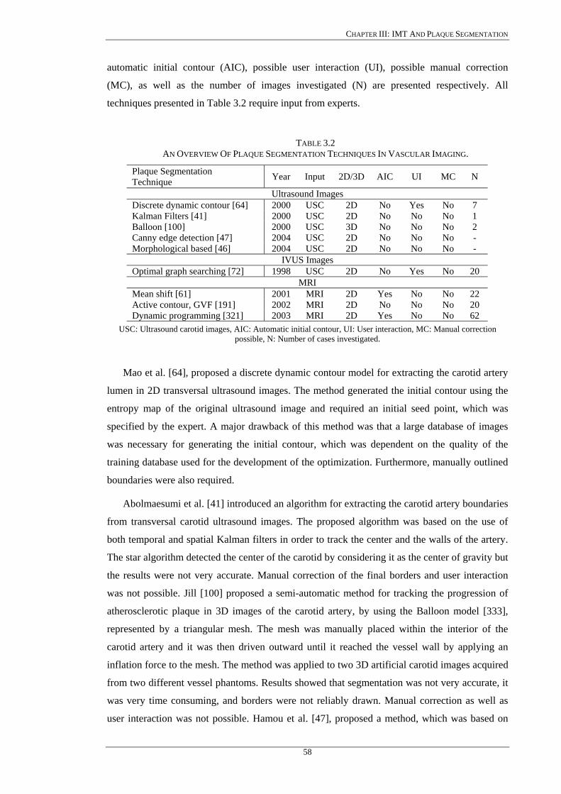
CHAPTER III: IMT AND PLAQUE SEGMENTATION
automatic initial contour (AIC), possible user interaction (UI), possible manual correction
(MC), as well as the number of images investigated (N) are presented respectively. All
techniques presented in Table 3.2 require input from experts.
TABLE 3.2 AN OVERVIEW OF PLAQUE SEGMENTATION TECHNIQUES IN VASCULAR IMAGING.
Plaque Segmentation Technique Year Input 2D/3D AIC UI MC N
Ultrasound Images Discrete dynamic contour [64] 2000 USC 2D No Yes No 7 Kalman Filters [41] 2000 USC 2D No No No 1 Balloon [100] 2000 USC 3D No No No 2 Canny edge detection [47] 2004 USC 2D No No No - Morphological based [46] 2004 USC 2D No No No -
IVUS Images Optimal graph searching [72] 1998 USC 2D No Yes No 20
MRI Mean shift [61] 2001 MRI 2D Yes No No 22 Active contour, GVF [191] 2002 MRI 2D No No No 20 Dynamic programming [321] 2003 MRI 2D Yes No No 62
USC: Ultrasound carotid images, AIC: Automatic initial contour, UI: User interaction, MC: Manual correction possible, N: Number of cases investigated.
Mao et al. [64], proposed a discrete dynamic contour model for extracting the carotid artery
lumen in 2D transversal ultrasound images. The method generated the initial contour using the
entropy map of the original ultrasound image and required an initial seed point, which was
specified by the expert. A major drawback of this method was that a large database of images
was necessary for generating the initial contour, which was dependent on the quality of the
training database used for the development of the optimization. Furthermore, manually outlined
boundaries were also required.
Abolmaesumi et al. [41] introduced an algorithm for extracting the carotid artery boundaries
from transversal carotid ultrasound images. The proposed algorithm was based on the use of
both temporal and spatial Kalman filters in order to track the center and the walls of the artery.
The star algorithm detected the center of the carotid by considering it as the center of gravity but
the results were not very accurate. Manual correction of the final borders and user interaction
was not possible. Jill [100] proposed a semi-automatic method for tracking the progression of
atherosclerotic plaque in 3D images of the carotid artery, by using the Balloon model [333],
represented by a triangular mesh. The mesh was manually placed within the interior of the
carotid artery and it was then driven outward until it reached the vessel wall by applying an
inflation force to the mesh. The method was applied to two 3D artificial carotid images acquired
from two different vessel phantoms. Results showed that segmentation was not very accurate, it
was very time consuming, and borders were not reliably drawn. Manual correction as well as
user interaction was not possible. Hamou et al. [47], proposed a method, which was based on
58
CHAPTER III: IMT AND PLAQUE SEGMENTATION
the canny edge detector to detect the plaque regions in carotid artery ultrasound images.
However, in the proposed method the expert had to specify three threshold parameters.
Furthermore, the proposed algorithm was not user friendly, and the accuracy of the results
depended to a large extent, on the appropriate selection of these threshold parameters.
Finally, a morphological based approach for the carotid contour extraction was proposed in
[46] for longitudinal ultrasound images of carotid artery, and this incorporated four different
stages. These were despeckle filtering, contour quantisation, morphological contour detection,
and a contour enhancement stage. The disadvantage of the method was that the expert had no
interaction with the system as all segmentation steps, which were made through morphological
processing, were predefined. Furthermore, the final plaque segmentation produced many small-
connected contours, showing all the edges of the carotid ultrasound image, instead of generating
a single closed loop contour indicating the plaque borders.
Other researchers used a graph-searching approach to detect the wall and plaque borders
from IVUS images of the carotid artery [72], [184]. The method was used to identify globally
optimal plaque borders, where initial information about the wall thickness, plaque location and
initial plaque borders was both required, and specified by the expert. The use of IVUS, poses a
certain risk to the patients, as discussed in Chapter 1, due to the insertion of a catheter in the
patient’s artery. Moreover, the system proposed in [72] required a sequence of IVUS images to
be provided. In addition, the method proposed in [72], and [184] was tested on 20 transversal
IVUS images of the carotid artery. In another study, Xu [61] applied a mean shift density
estimation algorithm to segment 22 multiple transversal MRI of the carotid artery. In this case,
the initial contour was estimated by finding the center of the gravity in the lumen area and
extending radial rays to the lumen border of the carotid artery. Results showed that the
segmentation was very time consuming, reliable borders were not drawn, and the segmentation
results were not compared with the hand outlined boundaries of experts. Other researchers have
attempted to segment the carotid plaque from vascular MRI, by using active contours based on
the GVF field, in order to detect the artery, lumen, and plaque borders [191], where the initial
contour was placed manually by the expert. The method was tested on 20 MRI images and the
results were compared with the manual delineations of one expert. Furthermore, the coefficient
of variation was also used in order to compare the manual with the GVF snakes segmented
boundaries. Yang [321] proposed a dynamic programming approach, to detect the plaque
borders in each MRI frame. The method was tested on 62 transversal MRI of the carotid artery
from six vessel specimens, and it was compared with the manual delineations of an expert. For
the estimation of the initial plaque contour, the expert was required to specify four seed points.
59
CHAPTER III: IMT AND PLAQUE SEGMENTATION
There are currently no other methods reported in the literature for accurately and
efficiently segmenting the plaque borders in ultrasound longitudinal images of the carotid
artery.
3.4 Active contours (snakes)
There has been a tremendous surge of interest in deformable templates in the context of
medical image analysis, where deformable models were used to segment anatomic structures
[352]. One of the earlier approaches to deformable template analysis [105], [332], was aimed to
find facial features for the purpose of recognition. Deformable templates evolve a shape to
match the image data. Earlier approaches were the HT [201], [204], and the WT [11], but they
require too many parameters, they have a high computational load, and generate over and under
segmentation results.
Active contours are curves that deform within digital images to recover object shapes [124],
[179], [243], [244], [259], [333]. They are classified as either parametric active contours (PACs)
or geometric active contours (GACs), according to their presentation and implementation. PACs
are represented explicitly as parameterized curves in a Lagrangian formulation [101], [179],
[240]. GACs are represented implicitly as level-sets of 2D distance functions, which evolve
according to an Eulerian formulation [60], [223]. They are based on the theory of curve
evolution implemented via level-set techniques [179], [239]. Current level-set techniques have
difficulties in representing open curves, as in our application for the segmentation of the IMT in
the carotid artery, while snakes are well suited for applications where open curves are required
[97], [111].
In 1988 Kass [243] introduced a new approach for locating features of interest in images,
called active contours or snakes, which was defined by an energy functional and a solution was
found using techniques of variational calculus and the finite difference methods [259]. The user
interactively specified the initial position of the snake [97]. Cohen [333] improved the above
method of Kass by using finite element methods, whereas C.-M. Chen [231], proposed a new
snake model with three important features, namely a modified-trimmed filter for noise
reduction, adaptive weighting parameters for weighting the third snake-energy term (see 3.4.2),
and edge enhancement by integration to capture the slowly varying edges. Williams&Shah
[124], improved the model proposed by Kass in [243], by incorporating a new energy continuity
term in (3.4.2), so that contour points were more evenly spaced, thus making the estimation of
the curvature more accurate. Amini [334] pointed out some of the problems of Kass’s approach
[243], including numerical instability and tendency for points to bunch up on strong portions of
an edge contour, by proposing dynamic programming. This approach was more stable and
allowed the inclusion of hard constraints inherent in the formulation of the functional however it
60
CHAPTER III: IMT AND PLAQUE SEGMENTATION
was slow having high complexity. Chang [205] proposed a 3D snake for malignant breast tumor
excision, where the image was first despeckled by anisotropic diffusion, and then estimated an
initial close snake contour for the tumor, using morphology operators. In all of the above
mentioned snakes segmentation approaches, snake requires that a close contour must be
detected. Snakes have been successfully employed in many other applications such as motion
tracking [7], [106], [240], [251], in medical images [7], [241], in facial image gesture [250], in
edge detection [243], shape modelling [216], segmentation [39], [44], [187], and in border
detection in artificial images [124], [116], [185].
Many modifications of the snake model have been proposed [7], [55], [64], [82], [253].
Recently Wang [260] proposed a modification of the ziplock snake [250], where multiple
contour features in artificial images were detected more accurately. Valvrede [108] applied
deformable models on nine mammogram images for vessel segmentation by defining a new
energy function associated with the image noise and avoiding the tendency of snake contour
points to bunch up. Other researchers proposed a pressure force [333], to solve the concave
problem, however, the details in determining the amplitude of force were not mentioned. Yuen
[252], combined the split and merge algorithm with the snake problem to overcome the problem
of the snakes initialization. Good results were obtained but this method was computationally
very expensive.
A snake is a parametric contour that deforms over a series of iterations. Each element
, along the snake contour depends on two parameters: namely , which is the space
(curve) parameter, and the , which is the time (iteration) parameter, and may be described as
[7]:
),( tsv s
t
. (3.4.1) ⎩⎨⎧
=parameteritterationtimetparametercurvespaces
tsv)(
)(),(
Internal forces, image forces, and external forces influence the snake contour, which evolves
as a set of points (contour) to match the image data. This set of points aims at fitting the target
feature to be extracted. A snake contour may be represented parametrically by
where , denotes the spatial coordinates of an image and
, represents the parametric domain (see also Fig. 3.2). The snake adapts itself by a
dynamic process that minimizes an energy function defined as [82], [124], [231], [243], [336]:
)],(),([)( sysxsv = 2),( ℜ∈yx
]1,0[∈s
61
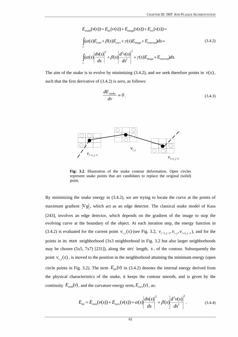
CHAPTER III: IMT AND PLAQUE SEGMENTATION
.))()()()()((
))()()((
))(())(())(())((
2
2
22
int
∫
∫
+++
=+++
=++=
sexternalimage
sexternalimagecurvcont
extimagesnake
dsEEsds
svdsds
sdvs
dsEEsEsEs
svEsvEsEsvE
γβα
γβα
ν
(3.4.2)
The aim of the snake is to evolve by minimizing (3.4.2), and we seek therefore points in ,
such that the first derivative of (3.4.2) is zero, as follows:
)(sv
0≡dv
dE snake. (3.4.3)
1,1 −− jivjiv ,
1,1 −+ jiv
Fig: 3.2. Illustration of the snake contour deformation. Open circles represent snake points that are candidates to replace the original (solid) point.
By minimizing the snake energy in (3.4.2), we are trying to locate the curve at the points of
maximum gradient g∇ , which act as an edge detector. The classical snake model of Kass
[243], involves an edge detector, which depends on the gradient of the image to stop the
evolving curve at the boundary of the object. At each iteration step, the energy function in
(3.4.2) is evaluated for the current point (see Fig. 3.2, ), and for the
points in its neighborhood (3x3 neighborhood in Fig. 3.2 but also larger neighborhoods
may be chosen (5x5, 7x7) [231]), along the length, , of the contour. Subsequently the
point , is moved to the position in the neighborhood attaining the minimum energy (open
circle points in Fig. 3.2). The term in (3.4.2) denotes the internal energy derived from
the physical characteristics of the snake, it keeps the contour smooth, and is given by the
continuity , and the curvature energy term, , as:
)(, sv ji 1,1,1,1 ,, −+−− jijiji vvv
mxnarc s
)(, sv ji
)(int vE
)(vEcont )(vEcurv
2
2
22
int)()()()())(())((
dssvds
dssdvssvEsvEE curvcont βα +=+= . (3.4.4)
62
CHAPTER III: IMT AND PLAQUE SEGMENTATION
3.4.1 Approximation of the first order differential
The continuity energy, , which is formed from the first order differential, )(vEcont dssdv )(
,
in (3.4.4), measures the energy due to stretching (elastic energy). It gives us the rate of change
for the length of the contour, which is the longitudinal contraction of the curve. It may be
formulated in discrete form, by calculating the average spacing between all the contour points,
which is the Euclidean distance, and then subtracting the distance between the current point and
the point before it as [124], [155] (see Fig. 3.2):
,)()()( 21,1,
21,1,
2
1,1,
2
−−−−−− −+−−=−−≈= jijijijijijicont yyxxdvvdds
sdvE (3.4.5)
where , is the average distance between snake points, , , are the current and the
precedent contour snake points, and , , , and , are the
d jiv , 1,1 −− jiv
jix , 1,1 −− jix jiy , 1,1 −− jiy yx, coordinates of
the contour snake points respectively. The term, 1,1, −−− jiji vv , is the distance between the two
snake contour points. Square values are used to avoid the square rooting thus speeding up the
calculations, and the continuity term is thus normalized to be in the range of [0, 1]. Points with a
distance between them, which is near the average distance between all contour points, will have
small values for . The average distance, , between points is calculated for every
iteration.
)(vEcont d
3.4.2 Approximation of the second order differential
The curvature term, , is formed from the second order differential, )(vEcurv 2
2 )(ds
svd, in
(3.4.4), and controls the contribution of the curvature energy due to point variation. It gives us
the convexity of the curve, and may be formulated in discrete form as [124], [155] (see Fig.
3.2):
,)2()2(
2)(
21,1,1,1
21,1,1,1
2
1,1,1,1
2
2
2
−+−−−+−−
−+−−
+−++−
=+−≈=
jijijijijiji
jijijicurv
yyyxxx
vvvds
svdE (3.4.6)
where , , , are the precedent, current, and next snake contour points, and
, , , , , , are the
1,1 −− jiv jiv , 1,1 −+ jiv
1,1 −− jix jix , 1,1 −+ jix 1,1 −− jiy jiy , 1,1 −+ jiy yx, coordinates of the contour snake
points respectively. Small values of (3.4.6) encourage the reduction of curvature, which forces
the contour to both maintain its shape and prevent the formation of corners. If corners or other
63
CHAPTER III: IMT AND PLAQUE SEGMENTATION
shape features are desired in the final result, )(sβ , which controls the natural behaviour of the
snake, can be adjusted accordingly to raise or lower the influence of curvature in the function
minimization. The internal energy in (3.4.2) contains a first-order term controlled by )(sα , and
a second order term controlled by )(sβ . The first order derivative discourages stretching and
makes the model behave like an elastic string by introducing tension. The second order
derivative discourages bending and makes the model behave like a rigid rod by producing
stiffness. The weighting parameters )(sα , and )(sβ , may be used to control the strength of the
model’s tension, and stiffness (rigidity), respectively. Low values of )(sα imply that the points
can change in spacing greatly. The weighting parameter )(sα controls how evenly spaced the
points in the contour will be, because is high for segments that are much shorter than or
much longer than the mean distance between points. Larger
intE
)(sα implies larger stretching, i.e.
the snake resists more in stretching. If )(sα is large, the snake tends to shrink (reduce length).
Also the smoothness of the snake increases. When 0)( =sα , then the points in the contour are
unevenly spaced, and eventually maybe placed on top of each other. The introduction of )(sα
allows smaller or larger contractions and therefore makes the snake act like an elastic string
[155], [243].
The term )(sβ controls the curvature of the contour. Large values of )(sβ may keep the
contour smooth except at corners, whereas low values imply that the curvature is not minimized
and the contour may form corners. It regulates the rate of change of the curve in the direction
normal to its boundary, and therefore it may be compared as a rigid string. High values
predispose the snake to smooth contours. If 0)( ≠sβ then the snake may better resist to
bending. The term )(sβ is progressively decreased around a corner until reaching a null value
at the exact corner location. If 0)( =sβ then it may develop corners.
Finally the term )(sγ , in (3.4.2) is a constant, and controls the influence of image gradients
on energy by balancing the image energy term, [231]. A large value of imageE )(sγ is useful in
making the curve converge faster.
The snakes segmentation algorithm determines first the energy for each snake point
according to (3.4.2), which are stored as the points with the minimum energy. This ensures that
if any other points are found to have equally or smaller energy, then the contour points will
remain the same. Then the local 3x3 neighbourhood, around each snake point, is searched to
determine whether any other point has a lower energy than the current contour point. If it does,
then that point is returned as the new contour point.
64
CHAPTER III: IMT AND PLAQUE SEGMENTATION
For the design of the snake model for extracting the intima and adventitia layer, the factors
)(sα , and )(sβ , are assumed to be dependent of position. For the calculation of )(sα , and
)(sβ , it is necessary to take into consideration the irregular spacing between the contour points
of the snake. This can be considered in the model by calculating the parameters )(sα , and
)(sβ , as follows [124], [246]:
2i
i hαα = , ,4
ii h
ββ = (3.4.7)
where , is the distance between the snake points , and . To control the mechanical
properties of the snake, the expert may also tune these parameters interactively. Both parameters
are determined by the demand of the application and the characteristics of objects. Note that
increasing both weighting factors may enhance the effect of the physical properties of the
model, and thereby diminish the influence of the external forces.
ih jiv , 1,1 −− jiv
Some other researchers proposed different formulations for the snake energy in (3.4.2),
where some other additional forces for characterizing the image features such as the Balloon
active model [333], the dual active contour model [242], the energy function in various
applications [249], and training on the-fly of the contour models by observing boundaries
accepted by the expert [226]. In [252] the internal energy of the snake, which was applied as a
close contour on artificial images, was modified by minimizing the area inside the snake instead
of minimizing the length of the snake contour.
3.4.3 Approximation of the image energy term
The term in (3.4.2), represents the image energy due to some relevant features
such as the gradient of edges, lines, regions [241], and texture [124], and some other forces
given by the user or based on the application. It attracts the snake to low-level features such as
brightness and edge data. The term, , is [116], [117], [179], [258]:
)(vEimage
)(vEimage
(3.4.8) ,))(())((1
0∫= dssvPsvE image
where , denotes a scalar potential function defined on the image plane. Another feature
of the image energy is the local gray level ratio between the outside and the inside of the
contour. Thus, the image force is chosen to be the gradient difference between the inside and the
outside of the contour, but it is set to zero during the contour deformation when the gray level
ratio between the outside and the inside of the contour is above a threshold. The gradient acts as
a driving force while the local gray level ratio plays a role as a stopping criterion to find the
))(( svP
65
CHAPTER III: IMT AND PLAQUE SEGMENTATION
location of inflation of the gray level profile. To apply snakes to images, image potentials are
designed whose local minima coincide with intensity extrema, edges and other image features of
interest. For example the contour will be better attracted to intensity edges in an image, , by
choosing a potential [241], [243], such that we convolve the image with a Gaussian function:
jig ,
,)*( ,,, jijiji gGcP σ∇−= (3.4.9)
where , controls the magnitude of the potential, c ∇ , is the gradient operator, and jiji gG ,, *σ ,
denotes the image convolved with a 2D Gaussian smoothing filter, jiG ,σ , whose characteristic
width, σ , controls the spatial extent of the local minima of P . Thus the image force may be
calculated by firstly normalizing the gradient magnitude in the range [0, 255]. The maximum
and the minimum gradient magnitude in the neighborhood of each snake point, , are then
evaluated as , and , respectively. If the dynamic range in the neighborhood is too
small (say smaller than 5) then the minimum is modified to be
jiv ,
maxg∇ ming∇
5maxmin −∇=∇ gg . The image
force for each neighborhood term may be then calculated as the re-normalized gradient [124]:
,)()(
minmax
,min
gggg
E jiimage ∇−∇
∇−∇= (3.4.10)
where , , are the minimum and maximum gradient values in the pixel snake
contour point neighborhood, and
ming∇ maxg∇
jig ,∇ , is the gradient value at the current location of the
observed snake contour point. The image energy term, , is in the range of [-1, 0] and is
more negative for large gradient values, so that contour points will be attracted to edges with
strong energy.
imageE
Equations (3.4.6) and (3.4.10) are normalized in the range of zero to one using the
maximum gradient value in the pixel neighborhood. The energy image term, , is already
normalized to this range as shown in (3.4.10). All terms constituting (3.4.2), are each multiplied
with their respective factors and then added together, as shown in (3.4.2), to form the energy
calculation for a specific contour location.
imageE
Some other implementations of the image energy, which depend on the application, were
reported in [116], where a new external force is introduced, called gradient vector flow (GVF),
which is computed as the diffusion of the gradient vector of the gray level or binary image
derived from the image. Xu [116], [117], applied the GVF method in one MRI and three
artificial images where the initialization was made manually and this posed a problem especially
when the snake is initialized far away from the boundary of interest. In addition this method had
66
CHAPTER III: IMT AND PLAQUE SEGMENTATION
difficulties, forcing a snake into long, and thin boundary indentations that was realized as a
close contour. A generalized formulation of the GVF (GGVF) was given in [258] concerning
the external force of the GVF snake, with an improvement in the convergence of the active
contour into long thin boundaries, but the snake was still implemented as a close contour.
Recently, an improvement of the GVF snake [116], [258], was reported for image video
sequences using multiscale GVF flow snakes [206] for vessel boundary tracking. Hamarneh
[119]-[121], developed an improved graphical user interface for segmenting images using the
active contour model. The method was applied on real world and medical ultrasound images but
the problem was still the placement of the initial snake contour, which had to be placed
manually by the expert. A new force in the energy functional (3.4.2) was additionally
introduced, where a number of parameters have to be set manually thus making the deformation
process very difficult.
3.4.4 Approximation of the external energy term
Finally the external snake energy term, , in (3.4.2), is user defined and optional
where many options are available [252]. In our application two external forces were used,
namely the line and the edge force described as:
)(vEexternal
edgeedgelinelineexternal EEvE ωω +=)( . (3.4.11)
The line functional, , in (3.4.11), generates forces that move the snake towards bright or
dark lines depending on the sign of
)(vEline
lineω , whereas in our implementation a negative value was
chosen in order to seek for a light line, which represents the bright echoes produced by the
adventitia layer. The term is expressed by, )(vEline jiline gvE ,)( = , which is the grayscale value
at the current snake contour point. Finally, the edge functional, , tries to lock the snake
within regions with large gradient values and is given by the negative of the squared magnitude
of the current contour point, , as:
)(vEedge
jig ,
2
,)( jiedge gvE ∇−= . (3.4.12)
3.5 Other snakes approaches
Most of the researchers have only investigated close snake contours [59], [60], [61], [225],
[226]. There are also open snake contours presented in the literature [241], [242], [250], [253],
[270], as also presented in this dissertation. These require a slightly different formulation from
the Kass [243], and the Williams&Shah [124] snake, and only minor modifications for
implementation. Snakes utilizing open contours use the same algorithm as snakes utilizing
67
CHAPTER III: IMT AND PLAQUE SEGMENTATION
closed contours, except that the starting and the ending points of the snake contour, may be
anchored as explained in Appendix IV.
One difficulty with the snakes segmentation algorithm is its sensitivity to noise due to its
local neighborhood action [108], [176]. Also, the snake algorithm can end up in an oscillatory
position where the final contour simply jumps between two equally attractive energy minima
[250], [304], [306]. One solution in resolving this difficulty is by increasing the size of the
snake neighborhood, but this incurs much greater complexity [248]. Another solution is to
despeckle the area, where the snake is applied, as proposed in [221], [231], [259], and in our
recent studies [154], [238], [335], [338]. In order to allow snakes to expand, a normal force can
be included which inflates the snake and pushes it over unattractive features [333]. The force
can be implemented by the addition of a normal force as:
),(snFnormal ρ= (3.5.1)
which is added to the snakes energy functional (3.4.2), where , is the normal force, and )(sn ρ
weights its effect. If the magnitude of the normal force is too large, it may force the contour to
pass over features of interest. Another way to allow expansion is to modify the elasticity
constraints so that the internal energy in (3.4.2) becomes [237]:
,)()()()()(2
2
222
int dssvdsL
dssdvsE βεα +⎟
⎟⎠
⎞⎜⎜⎝
⎛+−= (3.5.2)
where the length adjustment ε , when positive, 0>ε , and added to the contour length, ,
causes the contour to expand. When negative,
L
0<ε , this causes the contour length, , to
shrink and so the contour contracts.
L
Some snake approaches have included factors that attract contours to regions using
statistical models [244], or texture [245], to complement operators that combine edge detection
with region growing. Also the snake model can be generalized to higher dimensions and there
are 3D snake surfaces [246]. Finally an approach has introduced snakes for moving objects, by
including velocity [247].
3.5.1 Balloon snake
Cohen [333] introduced the Balloon snake model, whose internal energy causes it to expand
from inside of the boundary until it reaches it. He improved the original snake model by adding
a normalization force field term to the energy functional in (3.4.2), which may then be rewritten
by substituting the external field force as:
68

CHAPTER III: IMT AND PLAQUE SEGMENTATION
,)(1image
image
image
imageimage E
Eksnk
EEk
F∇
∇−=
∇
∇−= (3.5.3)
where , is a normal unity vector normal to the snake curve at point , and , is the
amplitude of this force. Cohen proposed, the addition of the term, , in (3.5.3), to the
force field, , which makes the contour have a more dynamic behavior, because he
observed that due to noise, some isolated points are gradient maxima and can stop the curve
when it passes by. The curve may be considered as a Balloon that is inflated. By changing the
sign of, , in (3.5.3), the curve will deflate instead of inflate. Now as the curve expands, it will
be attracted and stopped by edges as before, but since there is now a pressure force, if the edge
is too weak the curve may pass through without stopping at this point. If the curve runs into an
isolated point, it tends to create a tangent discontinuity at this point. The smoothing effect with
the help of the inflation force, removes the discontinuity and the curve may pass through the
edge.
)(sn )(sv 1k
)(1 snk
imageF
1k
3.5.2 Lai&Chin snake
Snakes have been formulated not only to include local shape, phrased in terms of
regularization [248], where a single parameter controls snake evolution, emphasizing a snakes
natural compromise between its own forces and the image forces. Regularization involves using
a single parameter to control the balance between the external and the internal forces. Given a
regularization parameter, πλ , the snake energy in (3.4.2) can be given as:
(3.5.4) .))}(()1())(({))((1
0 int dssvEsvEsvE imagessnake ππ λλ −+= ∫ =
If, the regularization parameter, 1=πλ , the snake will use only the internal energy, whereas if
0=πλ , the snake will be attracted only to the selected image function. Usually, regularization
concerns selecting a value between zero and one. The regularization parameter, which is
calculated at each contour, is given in as [248]:
,10 22
2
<+
=<ni
ni σσ
σλπ (3.5.5)
where , and , are the variance, and the noise variance at a snake point respectively,
and are bounded as [248]:
2iσ 2
nσ i
.11122 =+ni
σσ (3.5.6)
69
CHAPTER III: IMT AND PLAQUE SEGMENTATION
3.5.3 Gradient vector flow (GVF) snake
The GVF snake was originally introduced by Xu and Prince [116], [117], in order to
improve some poor properties, of the force field generated by the gradient operator, such as its
sensitivity to initialization, and its ability to move into concave boundaries where the following
conditions were enforced:
a) The gradient of an edge map, )),(( jiEext−∇ , has vectors pointing towards the edges,
which are normal to the edges at their location.
b) The vectors generally have large magnitude only in the immediate vicinity of the edges.
c) In homogeneous regions where the image is nearly constant, the gradient of the edge
map, )),(( jiEext−∇ , is nearly zero.
The overall approach is to use the force balance equation and introduce a new external force
field, , which is called GVF. The idea is based on the Helmholtz theorem [219],
which states that the most general static field can be decomposed into two components, namely
an irrotational (curl-free) and a solenoidal (divergence-free) component. In the classic case the
static field is irrotational, since it is the gradient of a potential function. A more general static
field may be obtained by allowing the possibility that it comprises both an irrotational and a
solenoidal component.
),( jivFext =
The external energy term, in the energy functional in (3.4.2) may be chosen differently, in
order to lead the snake toward step edges [117], [243] as:
,))(2
,1
jiexternal gvE ∇−= (3.5.7a)
,)*()(2
,,2
jijiexternal gGvE σ∇−= (3.5.7b)
where jiG ,σ , is a 2D Gaussian function with standard deviation, σ . If the image is a line
drawing (black on white), then the appropriate external forces include [333]:
(3.5.7c) ,)( ,3
jiexternal gvE =
(3.5.7d) .*)( ,,4
jijiexternal gGvE σ=
Variational calculus techniques are employed to minimize the energy functional in (3.4.2)
leading to the following Euler equations:
,0=−−di
dEii externalsssss βα .0=−−
djdEjj external
sssss βα (3.5.8a)
This can be viewed as a force balance equation:
70
CHAPTER III: IMT AND PLAQUE SEGMENTATION
(3.5.8b) ,0int =+ pexternalernal FF
where ssssernal biaiF −=int and . externalp
external EF −∇=
The overall approach is to use (3.5.8b) as a starting point for designing the snake. Replacing the
external forces ( ,/ didEexternal− ,/ djdEexternal− ) in (3.5.8a) in the ji, directions respectively,
with a vector field, , which is called GVF, we have [117]: ),( vu
,0))(),(( =+− sjsiuii sssss βα .0))(),(( =+− sjsivjj sssss βα (3.5.9)
The terms at a given position, , are determined by descending the following energy
functional [116], [117], [258]:
),( vu ),( ji
∫∫ ∫∫ −+−∇−++++∇= .))()(())(1())((),( 222222 didjfufufgdidjvvuufvuE jijijiGVF µ
with ,* ,,, jijiji gGf σ∇= and ),exp(GVFLffg ∇
−=∇ (3.5.10)
where , is a positive constant, which is used to control the smoothness of the resulting
vector field. The vector field guides the snake to the major boundaries. The parameter,
GVFL
µ , is a
regularization parameter governing the tradeoff between the first term and the second term in
the integrand. This parameter should be set according to the amount of noise present in the
image, where stronger noise implies an increased value of µ .
The solution to (3.5.8) can be obtained explicitly by the following iteration equations [117]:
0)),(),,((),( =+−= tsytsiuiitsx ssssst βα
0)),(),,((),( =+−= tsjtsivjjtsy ssssst βα (3.5.11)
where in these equations the active contour, )](),([)( sysxsv = , is treated as a function of time,
, as well as, , such as, t s )],(),,([),( tsytsxtsv = . In digital image processing the discrete
versions of (3.5.11) are used. For a complete discrete implementation of the GVF algorithm, see
[117].
3.6 Snake initialization
In this section, the initialization procedure for the IMT and plaque snake initial contour
estimation is described.
71
CHAPTER III: IMT AND PLAQUE SEGMENTATION
3.6.1 IMT contour initialization
It is important to place the initial snake contour as close as possible to the area of interest
otherwise the snake may be trapped in local minima or false edges, and converge to a wrong
location. The initial snake contour selection and the convergence are two of the main limitations
of the snake models proposed in the literature [55], [64], [124], [178], [185], [241], [243], [253].
Traditionally, most of the researchers used to place the initial contour by hand using the
experience of medical experts. This procedure was very cumbersome, tedious, expert dependent
and highly time consuming especially if a large database of images were to be segmented [93].
Various researchers proposed snake initialization methods in the past. Zahalka et al. [55]
proposed a method where an initial point was chosen in the middle of the lumen of a transversal
ultrasound image of the carotid artery. Radial rays 50 apart, were then calculated, which were
extended radialy outward from the initial point. Wendelhag et al. [253], proposed a dynamic
programming method with an initial estimation of the approximate positions of intima and
adventitia in longitudinal ultrasound images of the carotid artery. The initial boundaries were
then refined by a cost function containing image feature terms. Mojsilovic et al. [220] used a
fraction of image in runs measure (FOIIR) obtained with the gray-level run length method in
longitudinal ultrasound images. For the separation of the plaque and adventitia region the mean
gray level (MGL) was used. Liang et al. [178] performed fuzzy set theory for the initial snake
contour estimation where the approximate vessel wall positions were first estimated in a coarse-
scale image, which then guided the detection of the boundaries in a fine-scale image. Mao et al.
[64] estimated an initial contour for transversal ultrasound images to match the lumen of the
carotid artery initially with a circular contour.
Cheng et al. [241] located the adventitia border by placing manually on the gradient image
the starting and ending points of the initial contour. The procedure was performed for
longitudinal ultrasound images and the point selection had to be made above the intima in the
lumen area. Some other researchers [124], [185], [243], [336], estimated the initial snake
contour by hand or by placing the initial contour 10-20 pixels away from the desired boundary
[231]. Neuenschwander et al. [250] proposed the ziplock snake, which was an open contour
implementation, and it was initialized, by specifying a few points through which, the contour
must pass, thus minimizing the expert’s effort. The ziplock snake suffered from problems like
the initialization procedure, computational efficiency, and the location of concave and convex
parts of the object were not well detected. An initialization for the ziplock snake was proposed
recently [260], but still more than two points through which the contour passes must be
specified.
In another study, Yuen et al. [252] located the initial snake contour in artificial images, by
using the center of gravity of the object and extented radial vertical lines from center to the
72
CHAPTER III: IMT AND PLAQUE SEGMENTATION
perimeter searching for the points with the maximum gradient. Some other researchers used the
GHT [203] for the snake initialisation but it was shown not to be very accurate and was very
time consuming [248].
Still other researchers [242], tried to solve some of the problems connected with the snake
initialization by using a dual contour approach. In this approach, the two contours were
deformed in such a way, so that they could not be attracted together, and so that they enclosed
the target shape with an inner and an outer contour. The disadvantage of this approach was that
the shape of interest could not be located accurately, as the snake contours were deformed in
predefined directions.
All the above methods involved expert dependence, some of them required parameter
initialization which had to be chosen empirically, some were applied to artificial images and
only a few were proposed for ultrasound images.
The IMT snakes initialization method proposed in this dissertation, (see Chapter 5.7.2),
requires minimum expert interaction, is not expert dependent and is an open snake contour
implementation.
3.6.2 Plaque contour initialization
In the literature, very few approaches have been proposed for segmenting the atherosclerotic
carotid plaque from ultrasound images, where the initial contour was placed manually by the
user [46], [47], [53], [100], [192]. A method for segmenting the arterial walls and plaque from
transversal MRI images based on dynamic programming was proposed in [321], where the
initial contour was found by manually placing four points on the artery walls. There are no other
studies reported in the literature, where an initialisation procedure was proposed for extracting
the borders of the carotid atherosclerotic plaque in longitudinal ultrasound images.
In this work we propose an initialisation procedure for detecting the initial plaque borders in
the carotid artery, which is described in Chapter 5.8.2.
73

CHAPTER IV: IMAGE QUALITY, TEXTURE ANALYSIS, AND ROC ANALYSIS
Chapter 4
Image Quality, Texture Analysis, And ROC Analysis
74
CHAPTER IV: IMAGE QUALITY, TEXTURE ANALYSIS, AND ROC ANALYSIS
Chapter 4: Image Quality, Texture Analysis, And ROC Analysis
Image quality plays an important role in various image-processing applications. A great deal
of effort has been made in recent years to develop objective image quality and segmentation
measures that correlate well with perceived quality measurements. However, only limited
progress has been made. In this Chapter, we define various image quality, texture measures and
receiver operating characteristics (ROC) measures, which may be used to evaluate the despeckle
filtering and segmentation techniques, presented in Chapter 2 and Chapter 3 respectively.
4.1 Image quality
When is an image good or bad? A straightforward definition of image quality is based on the
question: How well does an image communicate information required by an expert? This is
called the intelligibility of the image or the diagnostic image quality [273]. A more technical
definition of image quality relates to the question: How much does an image deviate from an
ideal image or scene? This is called the fidelity of an image or technical image quality. Both
aspects may be determined by comparing the processed images with the ground truth.
Ultrasound is subject to a number of artefacts that degrade image quality and compromise
diagnostic confidence [128], [160]. For medical images, quality can be objectively defined in
terms of performance in clinically relevant tasks such as lesion detection and classification
[329]. For applications in which images are ultimately to be viewed by human experts, the only
correct method of quantifying visual image quality is through objective evaluation. In practice,
however, objective evaluation is usually too inconvenient, time consuming and expensive. The
goal of research in image quality is to define and develop quantitative measures that can
automatically predict perceived image quality.
Traditionally the ROC analysis was the dominant technique for evaluating image quality,
where a subjective image quality index can be evaluated from the area under the ROC curves
[363]. To construct a typical ROC study a large number of images are required to be evaluated
in order to obtain a statistically significant result [300]. Usually in ROC studies, experts are
asked to review the images before and after processing in order to provide a yes or no decision.
The wide spread of mobile and portable telemedicine ultrasound scanning instruments also
necessitates the need for better image processing techniques, in order to offer a clearer image to
the medical practitioner, and transfer the image with the minimum loss of quality. This makes
the use of efficient image quality evaluation criteria an important task [174].
An objective image quality metric can play an important role in a broad range of applications.
First, it may be used to dynamically monitor and adjust image quality. Second it may be used to
optimise algorithms and parameter settings of image processing systems [278]. For instance, a
75
CHAPTER IV: IMAGE QUALITY, TEXTURE ANALYSIS, AND ROC ANALYSIS
quality metric can assist in the optimal design of a despeckle filter. Objective image quality
measures can be classified according to the availability of an original image (noise image), with
which the despeckled image is to be compared. Most existing approaches are known as full-
reference, meaning that a complete reference image is available. In some practical applications,
however, the reference image is not available, and a no-reference or blind quality assessment
approach is desirable. In a third type of method the reference image is only partially available in
the form of a set of extracted features made available as side information to help evaluate the
quality of the despeckled image. In our case of the ultrasound longitudinal images of the carotid
artery are readily available. The despeckling process will help the expert to perform a more
accurate and error free diagnosis. Therefore we will focus in this work on full-reference image
quality assessment measurements.
A lot of researchers have tried in the past to develop quality assessment methods that utilise
the known characteristics of the human visual system (HVS). It is generally easy for the HVS to
assess the quality of two similar images and decide on which one looks better. In [361] image
quality metrics are separated into the three categories:
a) Human perception: In this category a selected group of viewers evaluate a range of
images according to their subjective criteria. It involves measuring the performance of a
display device by measuring the ability of the expert to perform a task using that device.
The advantage is that it may be applied even in the absence of any reliable model. The
major disadvantages are, cost of data collection, it is very time consuming, and the large
amount of cases needed for the evaluation.
b) Objective measures based on theoretical models: In this category mathematically based
theoretical models are used to take advantage of the fact that images can be represented as
a matrix of numerical values. One may then apply some transformations to these
matrices. These measures are still very attractive because they are easy to calculate, have
usually low complexity, and they are independent of viewing conditions and individual
experts.
c) Subjective measures based on mathematically defined models of the HVS: The functional
components of the HVS are very difficult to be implemented, so the measures belonging
to this category are the most difficult to implement.
In this study human perception evaluation was carried and objective measures were
extracted for evaluating the results of depeckle filtering and segmentation techniques.
4.2 Optical perception testing procedures
In order to be able to design accurate and reliable quality metrics, it is necessary to
understand what quality means to the expert. An expert’s satisfaction when watching an image
76
CHAPTER IV: IMAGE QUALITY, TEXTURE ANALYSIS, AND ROC ANALYSIS
depends on many parameters, such as: viewing distance, display size, resolution, brightness,
contrast, sharpness, colourfulness, naturalness, and other factors [284], [285], [291].
It is also important to note that there is often a difference between fidelity (the accurate
reproduction of the original on the display), and perceived quality. Sharp images with high
contrast are usually more appealing to the average expert. Likewise, subjects prefer slightly
more colourful and saturated images despite realizing that they look somewhat unnatural [292].
For studying visual quality some of the definitions above should be related to the HVS. For
instance, it is very popular between medical image experts to specify viewing distance in terms
of display size, i.e. in multiples of screen height. The ratio of the preferred viewing distance to
screen height is usually constant [293]. However, recent experiments with larger displays
showed that this might not be the case. While the preferred viewing distance is indeed around 6
to 7 screen heights for smaller displays, it approaches 3 to 4 screen heights with increasing
display size [293].
Unfortunately, subjective quality may not be described by an exact figure, due to its inherent
subjectivity, it can only be described statistically. Even in psychological threshold experiments,
where the task of the expert is to give a yes or no answer, there exists a significant variation
between experts, contrast sensitivity functions, and other critical low-level visual parameters
[287]-[293]. When speckle noise is apparent in the image, the expert’s differing experiences
with noise are bound to lead to different weightings of the artifact [286]. Researchers showed
that experts and non-experts (with respect to image quality) examine different critical image
characteristics to form their final opinion [286], [291]. In light of these difficulties, testing
procedures for subjective quality assessment are discussed in detail in Appendix II.
The visual perception evaluation, in this study, was carried out according to the ITU-R
recommendations similar with the Double Stimulus Continuous Quality Scale (DSCQS)
procedure [316] (see also Appendix II). The presentation sequence for a DSCQS trial is shown
in Fig. 4.1a. Experts are shown multiple sequence pairs consisting of a reference (Ref.) and a
test sequence (Test), which are rather short (typically 10 seconds). The reference and test
sequence are presented twice in alternating fashion, with the order of the two chosen randomly
for each trial. Experts are not informed which is the reference and which is the test sequence.
They rate each of the two separately on a continuous quality scale ranging from bad to excellent
as shown in Fig. 4.1b. Analysis is based on the difference in rating for each pair, which is
calculated from an equivalent numerical scale from 1 to 100. This differencing removes a lot of
the subjectivity with respect to scene content and experience. It is noted that in this study the
observation time was not limited to 10 seconds, as in the DSCQS method, but we have allowed
the experts to observe the image for as long as they wanted, and were also able to go back and
forth to observe the images.
77

CHAPTER IV: IMAGE QUALITY, TEXTURE ANALYSIS, AND ROC ANALYSIS
(a) Presentation Sequence
Ref. Test Ref. Test Vote
Ref. Test
100 Excellent
Good
Fair
Poor
0 Bad
(b) Rating Scale
Fig. 4.1: DSCQS method: (a) the reference and the test sequence are presented twice in alternated fashion, (b) the order of the two is chosen randomly for each trial, and experts are not informed which is which. They rate each of the two separately on a continuous quality scale ranging from bad to excellent (Modified from [7] pp. 572, Fig. 10.1).
4.3 Image quality metrics
In this section we propose a number of image quality metrics, that can be used for
objectively evaluating the despeckle filters proposed in Chapter 2. Differences between images
were evaluated using the following image quality evaluation metrics, which were used as
statistical measures, between the original noisy image, , and the despeckled, , image. jig , jif ,
a) The normalised mean square error MSE:
∑∑= =
−=
M
i
N
j ji
jiji
lpgfg
MNMSE
1 1
2
,
,, )(1 (4.1)
which measures the quality change between the original, , and the despeckled image,
, in an
jif ,
jig , MxN window [300]. The , is the low pass filtered of the original image,
. In case that, , is equal zero, its value is replaced with the smallest gray level
value in the image. The , has been widely used to quantify image quality and when is
used alone, it does not correlate strongly enough with perceptual quality. It should be used
therefore together with other quality metrics and visual perception [294], [300].
jilpg ,
jig , jilpg ,
MSE
b) The normalised root mean square error, RMSE, which is the square root of the squared
error averaged over the MxN array [3]:
∑∑= =
−=
M
i
N
j ji
jiji
lpgfg
MNRMSE
1 1
2
,
,, )(1 . (4.2)
78
CHAPTER IV: IMAGE QUALITY, TEXTURE ANALYSIS, AND ROC ANALYSIS
The popularity of arises mostly from the fact that is in general the best
approximation of the standard error.
RMSE
c) The normalised error summation in the form of the Minkowski metric, which is the
norm of the dissimilarity between two images, as follows [272], [278], [287], [300]:
ββ /1
1 ,
,,
1
1⎟⎟
⎠
⎞
⎜⎜
⎝
⎛ −= ∑∑
==
N
j ji
jijiM
i lpgfg
MNErr (4.3)
with 41 << errβ . For 2=errβ , one obtains the RMSE expression in (4.2), whereas for
1=errβ , the absolute difference, and for ∞=errβ , the maximum difference measure.
d) The normalised geometric average error, GAE , is a measure, which shows if the
despeckled image is very bad [316], and it is used to replace or complete the . It
is positive only if every pixel value is different between the original and the despeckled
image. The GAE , is zero, if there is a very good transformation between the original
and the despeckled image, and high if the transformation with the original is extremely
bad. This measure is also used for tele-ultrasound, when transmitting ultrasound images
and is defined as:
RMSE
NMN
i
M
jji
jiji
lpgfg
GAE /11 1
,
,, )(∏ ∏= =
−= . (4.4)
The may be used to replace the , which is dominated by its large
individual terms and is calculated for an image with dimensions . This amounts
to a severe error in when large individual terms are present. For this reason the
is often replaced by the GAE.
GAE RMSENXM
RMSERMSE
e) While signal sensitivity and image noise properties are important by themselves, it is
really the ratio of them that carries the most significance. The normalised SNR [133]
pp. 169-170, [331] is defined as:
∑∑
∑∑
= =
= =
−
+
= M
i
N
j ji
jiji
M
i
N
j ji
jiji
lpgfg
lpgfg
SNR
1 1
2
,
,,
1 1 ,
2,
2,
10
)(
)(log10 . (4.5)
It is calculated over an image area with dimensions . The , , and NXM SNR RMSEErr , prove to be very sensitive tests for image degradation, but there are completely
non-specific. Any small change, in image noise, despeckling, and transmitting
preferences would cause an increase of the above measures.
79
CHAPTER IV: IMAGE QUALITY, TEXTURE ANALYSIS, AND ROC ANALYSIS
f) The normalised peak signal to noise ratio, PSNR, is defined as [331]:
2max
10log10sMSEPSNR −= (4.6)
where , is the maximum pixel value in the image. The , is higher for a
better-despeckled image and lower for a poorly despeckled image. It measures image
fidelity that is how closely an image (despeckle) resembles usually the corrupted
original.
maxs PSNR
g) The mathematically defined universal quality index, Q, [272] models any distortion as a
combination of three different factors, which are, loss of correlation, luminance
distortion, and contrast distortion. The Q is defined as:
2222
2)()(
2
gf
gf
gf
gf
gfgfQ
σσσσ
σσσ
++= , 11 <<− Q (4.7)
where g , and f , represent the mean of the original and despeckled image values, with
their standard deviations, ,gσ and ,fσ of the analysis window, and gfσ , represents the
covariance between the original and transformed images. Q is computed for a sliding
window of size 8x8 without overlapping. Its highest value is 1 and is achieved when
both images are identical ( jiji fg ,, = ), while its lowest value is –1 for jiji ggf ,, 2 −= .
h) The structural similarity index, SSIN, between two images [278], is a generalization of
(4.7) and is defined as:
))((
)2)(2(
2sin_22
1sin_22
2sin_1sin_
sfgs
sgfs
ccfgccfg
SSIN++++
++=
σσσ
, 11 <<− Q (4.8)
where , , are constants. The Q, defined in g), corresponds to the special
case that in (4.8),
1sin_sc 2sin_sc
02sin_1sin_ == ss cc , which produces unstable results when either
)( 22 fg + or , is very close to zero. The range of values for the lies
between –1, for a bad and 1, for a good similarity between the original and the
despeckled images respectively. It is computed, similarly to the measure, for a
sliding window of size 8x8 without overlapping.
)( 22fg σσ + SSIN
Q
i) The speckle index, C, [131] for log-compressed ultrasound images is defined as:
∑∑= =
=M
i
N
j ji
ji
MNC
1 1 ,
,21µσ
(4.9)
80
CHAPTER IV: IMAGE QUALITY, TEXTURE ANALYSIS, AND ROC ANALYSIS
and is an average measure of the amount of speckle presented in the image area with size
MxN , as a whole (over the whole image). It is used in most adaptive filters to adjust the
weighting function , in (2.3.1), described in section 2, because it reflects the changes in
contrast of the image in the presence of speckle noise. It does not depend on the intensity of
the local mean but on the variance, , and the mean,
jik ,
2σ µ , of the whole image. The larger C
is, the more likely that the observed neighbourhood belongs to an edge, thus C may be used
also as an edge detector.
j) Lesions detectability can be quantified using the contrast-to-speckle ratio, CSR [199].
It is calculated by defining two regions of interest (i.e. the original image and the
despeckled), and using the mean pixel value, and the variance, to quantify the contrast,
121 /)( µµµ − , and the speckle index noise, 122
21 /)( µσσ + . The ratio of these two
quantities is termed as CSR and is defined as:
)(/))(( 22
21121 σσµµµ +−=CSR (4.10)
where ,1µ ,2µ ,1σ ,2σ are the mean and standard deviations of the original and
despeckle images respectively. The , provides a quantitative measure of the
detectability of low contrast lesions, when one region is completely inside the lesion
and the second is the background media.
CSR
The quality measures proposed above, do not necessarily correspond to all aspects of the
expert’s visual perception of the errors, nor do they correctly reflect structural coding artefacts
[283], but if they are all combined together, and with the subjective tests, may offer a more
accurate evaluation result. Subjective tests are tedious, time consuming and expensive, and the
results depend on the expert’s background, motivation, and other factors [272], [273], [284].
However, all these measures cover the visual quality just partly. The visual quality of an image
is difficult to define with mathematical precision, since it is dependent on the properties of our
visual system. We know, for example, that our visual system is more tolerant to a certain
amount of noise than to a reduced sharpness. On the other hand it is very sensitive to certain
specific artefacts, like blips and bumps [294].
4.4 Texture analysis
Following the despeckling, texture features may be extracted from the original and the
despeckled images in order to be used for texture analysis. Texture analysis is one of the most
important features used in image processing and pattern recognition. It can provide information
about the arrangement and spatial properties of fundamental image elements. Many methods
81
CHAPTER IV: IMAGE QUALITY, TEXTURE ANALYSIS, AND ROC ANALYSIS
have been proposed to extract texture features, e.g. the co-occurrence matrix [262], and the
texture spectrum in the achromatic component of the image [263].
4.4.1 Texture measures
Some of the most common texture feature algorithms that have been used for ultrasound
texture analysis are: simple statistical features (SF), spatial gray level dependence matrices
(SGLDM) [128], gray level difference statistics (GLDS) [129], neighbourhood gray tone
difference matrix (NGTDM) [214], statistical feature matrix (SFM) [213], laws texture energy
measures (TEM) [211], [212], fractal dimension texture analysis (FDTA) [210], [211], and
Fourier power spectrum (FPS) [129]. These texture features are usually computed on a region
of interest, for example the region prescribed by the plaque contour that is automatically or
manually drawn.
The SF includes the µ , median, , , and values. The SGLDM, texture features as
proposed by Haralick et al. [128], are the most frequently used texture features. These are based
on the estimation of the second-order joint conditional probability density functions that two
pixel pairs, (k, l) and (m, n), with distance, d, in direction specified by the angle, θ, have
intensities of gray level,
2σ 3σ 4σ
g , and gray level, . Based on the probability density functions, the
following texture measures, and their variants [128] are computed: angular second moment
(ASM), contrast, correlation, inverse difference moment (IDM), sum average, variance (sum
and difference), and entropy (sum and difference). For a chosen distance, d, that is usually one
pixel and for angles, and , four values for each of the above texture
measures are computed. The mean and range of these four values are usually computed for
each feature, and they are used as two different feature sets. The GLDS algorithm [129], uses
first order statistics of local property values based on absolute differences between pairs of gray
levels or of average gray levels in order to extract the following texture measures: contrast,
ASM, entropy, and mean. Amadasun and King [214] proposed the NGTDM, in order to extract
textural features, which correspond to visual properties of texture. The following features are
extracted: coarseness, contrast, busyness, complexity, and strength. The FDTA is based on the
work of Mandelbrot [210], who developed the fractional Brownian motion model in order to
describe the roughness of natural surfaces. The Hurst coefficients (
f
000 90,45,0=θ 0135
)(kH ) [211], are computed
for different image resolutions, where a smooth texture-surface is described by a large value of
the parameter, )(kH , whereas the reverse applies for a rough texture-surface. The FPS,
computes the radial and angular sum of the sample FPS, where coarse texture has high values
concentrated near the origin, and in fine texture the values are more spread out. The 56 different
texture measures used in this study are further described in the Appendix III.
82
CHAPTER IV: IMAGE QUALITY, TEXTURE ANALYSIS, AND ROC ANALYSIS
4.4.2 Feature selection
In order to identify the most discriminant features for the classification task (features that
have the highest discriminatory power), the distance between asymptomatic and symptomatic
images was calculated for the set of all ultrasound images, before and after despeckle filtering
for each feature as follows [10], [131]:
)(/ 22
12
21, iiiici mmdis σσ +−= (4.11)
where , is the feature index, , if o , indicates the original image set and if , indicates the
despeckled image set, , and , are the mean values and
i c f
1im 2im 1iσ , and 2iσ , are the standard
deviations of the asymptomatic and symptomatic classes respectively. The most discriminant
features are the ones with the greatest distance values [10]. If the distance after despeckle
filtering is increased i.e.:
ioif disdis > (4.12)
then it can be derived that the classes may be better separated.
For each feature, a percentage distance was computed as:
100)(_ ioifi disdisdisfeat −= . (4.13)
For each feature set, a score distance was computed as:
(4.14) 100)()/1(_1∑=
−=featN
iioiffeat disdisNDisScore
where , is the number of features in the feature set. It should be noted that for all features a
larger feature value shows improvement.
featN
The Wilcoxon rank sum test was also used in order to identify if for each texture feature a
significant (S) difference or not (NS) exists between the original and the despeckled images at
p<0.05.
4.4.3 kNN Classifier
The statistical pattern recognition k-nearest-neighbour (kNN) classifier with 7=k , was
used to classify a plaque as asymptomatic or symptomatic [10], [132]. The kNN classifier was
chosen because it is simple to implement and computationally very efficient. This is highly
desired due to the many feature sets and filters tested [211].
In the kNN algorithm in order to classify a new pattern, its k-nearest-neighbours from the
training set, are identified. The new pattern is classified to the most frequent class among its
83

CHAPTER IV: IMAGE QUALITY, TEXTURE ANALYSIS, AND ROC ANALYSIS
neighbours based on a similarity measure that is usually the Euclidean distance. In this work the
kNN carotid plaque classification system was implemented for values of 1, 3, 5, 7 and 9
using for input the eight texture feature sets and morphology features described above.
=k
The leave-one-out method was used for evaluating the performance of the classifier, where
each case is evaluated in relation to the rest of the cases, characterized by no bias concerning the
possible training and evaluation bootstrap sets. This method calculates the error or the
classifications score by using 1−n samples in the training set and testing or evaluating the
performance of the classifier on the remaining sample. It is known that for large n , this method
is computationally expensive. However, it is approximately unbiased, at the expense of an
increase in the variance of the estimator [144].
4.5 ROC analysis
In this section we focus on the problem of measuring the performance of medical image
segmentation techniques by taking into consideration the ROC analysis, which describes the
subjective performance of an expert. Our aim is to be able to make meaningful statements of the
form-“Algorithm A performs better than algorithm B at detecting the IMT or plaque
boundaries” or “Algorithm A performs better than the medical expert does”. Performance
metrics of this type are of course very complex than those for abnormality detection problems.
In the following sections, performance metrics for measurement problems and for image
segmentation are defined.
4.5.1 Performance metrics for detection problems
When the goal is to estimate the value of some scalar or vector quantity, it is natural to focus
on the difference between the calculated result (automatic segmentation), and some independent
measure of the true value (manual segmentation). Because the absolute value of the difference
typically varies with the size of the true value, it is typical to focus on a mean relative error [7],
[363]:
onsegmentatimanualonsegmentatimanualonsegmentatiautomaticerrorrelativemean
_)_()_(__ −
= , (4.15)
where automatic, and manual segmentation represent the snakes segmented, and manually
segmented boundaries respectively.
The metrics presented in this section, include the relative frequency of correct and incorrect
decisions. In the context of detecting the presence of an abnormality in an image, the terms true
positive (TP), false positive (FP), true negative (TN), and false negative (FN), are commonly
used [7], [363]. The above definitions are explained below and summarized in Fig. 4.2 as
follows:
84

CHAPTER IV: IMAGE QUALITY, TEXTURE ANALYSIS, AND ROC ANALYSIS
Algorithm Decision
Abnormality present
Abnormality not present
Abnormality
present TP FN Truth of
clinical
Situation Abnormality
not present FP TN
Fig. 4.2: Definition of TP, FN, FP, and TN.
TP: The abnormality is actually present and the expert as well as the segmentation
algorithm, correctly identifies as so.
TN: The abnormality is absent and the expert as well as the segmentation algorithm, decides
that an abnormality is absent.
FP: The abnormality is not actually present according to the expert, and the segmentation
algorithm, incorrectly decides that it is.
FN: The abnormality is present according the expert, and the segmentation algorithm,
incorrectly decides that it is absent.
Several additional performance metrics are derived from the TP, FN, FP, and TN. The
sensitivity of a detection algorithm refers to how frequently the algorithm report that an
abnormality exists in the instances where one actually does exist. Sensitivity can be stated as a
fraction between 0 and 1, or as a percentage between 0 and 100.
The definition of sensitivity (or recall) [39] can be stated in terms of the number of TP and
FN. By definition, the sum of the TP and FN is the set of all instances where an abnormality
exists. Thus, the sensitivity, R , is given as [7]:
TPFFNTP
TPR =+
=)(
, 10 ≤≤ R . (4.16)
The R , can range from a low of 0, indicating that none of the abnormalities are detected, to
a high of 1 (or 100 percent), indicating that all of the abnormalities are detected. The true
positive fraction, TPF is the same as the sensitivity, R .
The specificity, , of a detection algorithm refers to how frequently it correctly reports
normal when no abnormality exists. As with
Sp
R , , is also stated as a fraction between 0 and Sp
85

CHAPTER IV: IMAGE QUALITY, TEXTURE ANALYSIS, AND ROC ANALYSIS
1, or as a percentage between 0 and 100. The definition of , can be stated in terms of the
numbers of TN and FP. By definition, the sum of the TN and the FP is the set of all normal
instances. Thus, is given as:
Sp
Sp
FPFFPTN
TNSp −=+
= 1)(
, 10 ≤≤ Sp . (4.17)
An , of 1 would indicate that every normal instance is reported as normal. The false positive
fraction, FPF, is the same as,
Sp
Sp−1 which is the fraction of the normal cases that is falsely
reported as abnormal.
The ideal detection algorithm would have both, an R , and , of 1 (or 100 percent). This
would imply finding the abnormality in every instance where one existed, and never falsely
saying that an abnormality existed. Of course, one generally cannot expect to achieve such
perfection in practice.
Sp
Precision, P , [39] measures the proportion of the nominated positive examples that are
correct as:
)( FPFTPF
TPFP+
= , 10 ≤≤ P (4.18)
Stating only one of the R , and , for an algorithm is generally meaningless. A perfect Sp R ,
is easily achieved by a detection algorithm, which always decides that an abnormality exists. A
perfect , is easily achieved by a detection algorithm that never decides that an abnormality
exists. In the typical situation, greater
Sp
R , can be gained by accepting lower , and vice versa.
To determine if one technique outperforms another, it is useful to combine the above measures
into a single measure of goodness, which is the effectiveness measure,
Sp
E , [39], which is
proposed as:
RP
PREαα +−
−=)1(
1 , 10 ≤≤ E (4.19)
where , and )1/(1 2 += βα E , is β times more heavily weighted towards R , than P . In this
work, P , and R , are equally weighted ( 1=β ). Since E , is an inverse measure of goodness,
we will generally quote segmentation performance in terms of EF −=1 , in what follows.
Ideally, the snakes segmentation method should have a 100% score for all above statistics.
A 100% score for the R , indicates that the method detects all plaque pixels. A 100% score for
the , would indicate that it never detects a plaque pixels in a non-plaque zone. Sp
86
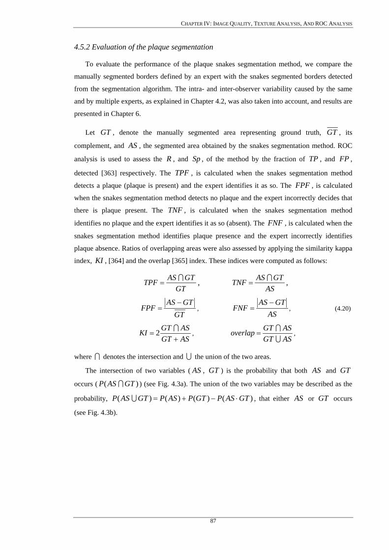
CHAPTER IV: IMAGE QUALITY, TEXTURE ANALYSIS, AND ROC ANALYSIS
4.5.2 Evaluation of the plaque segmentation
To evaluate the performance of the plaque snakes segmentation method, we compare the
manually segmented borders defined by an expert with the snakes segmented borders detected
from the segmentation algorithm. The intra- and inter-observer variability caused by the same
and by multiple experts, as explained in Chapter 4.2, was also taken into account, and results are
presented in Chapter 6.
Let , denote the manually segmented area representing ground truth, GT GT , its
complement, and , the segmented area obtained by the snakes segmentation method. ROC
analysis is used to assess the
AS
R , and , of the method by the fraction of TSp P , and FP ,
detected [363] respectively. The TPF , is calculated when the snakes segmentation method
detects a plaque (plaque is present) and the expert identifies it as so. The FPF , is calculated
when the snakes segmentation method detects no plaque and the expert incorrectly decides that
there is plaque present. The TNF , is calculated when the snakes segmentation method
identifies no plaque and the expert identifies it as so (absent). The FNF , is calculated when the
snakes segmentation method identifies plaque presence and the expert incorrectly identifies
plaque absence. Ratios of overlapping areas were also assessed by applying the similarity kappa
index, KI , [364] and the overlap [365] index. These indices were computed as follows:
GT
GTASTPF I= ,
ASGTASTNF I
= ,
GT
GTASFPF
−= ,
ASGTAS
FNF−
= , (4.20)
ASGTASGTKI
+=
I2 , ASGTASGToverlap
U
I= ,
where denotes the intersection and U the union of the two areas. I
The intersection of two variables ( , ) is the probability that both and
occurs ( ) (see Fig. 4.3a). The union of the two variables may be described as the
probability,
AS GT AS GT
)( GTASP I
)()()()( GTASPGTPASPGTASP ⋅−+=U , that either or GT occurs
(see Fig. 4.3b).
AS
87
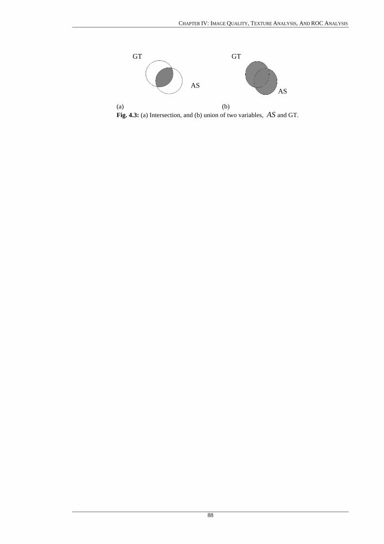
CHAPTER IV: IMAGE QUALITY, TEXTURE ANALYSIS, AND ROC ANALYSIS
TGT
S
AS
(a) (b) Fig. 4.3: (a) Intersection, and (b) union of two variables, and GT. AS
88
A
G

CHAPTER V: METHODOLOGY
Chapter 5
Methodology
89
CHAPTER V: METHODOLOGY
CHAPTER 5: METHODOLOGY
In this Chapter, we present the methodology of our work, where the material used, the
ultrasound scanners for acquiring the ultrasound images, the process of recording the ultrasound
images, image normalisation, generation of an artificial carotid image, despeckle filtering, the
procedure followed by the two experts for the visual perception evaluation, texture analysis, and
image quality evaluation metrics, are presented respectively. Furthermore, the manual
segmentation procedure for the IMT, visual perception evaluation for the snakes segmentation,
the snakes segmentation procedure for the IMT, univariate statistical analysis and correlation
analysis are presented respectively. In Chapter 5.8 the protocol for the manual segmentation
procedure for the plaque, visual perception evaluation, the snakes segmentation for plaque with
four different snake algorithms, and the evaluation of the plaque segmentation methods are
presented respectively.
5.1 Material
Four imaging datasets were used in this study. The first imaging dataset was used for
evaluating the image quality of two ultrasound scanners, the second for evaluating despeckle
filtering, the third for segmenting the IMT, and the fourth for plaque segmentation.
The first image dataset was collected at the Cyprus Institute of Neurology and Genetics,
using an ATL (model HDI-3000 Advanced Technology Laboratories, Seattle, USA) and an
ATL (model HDI-5000 Advanced Technology Laboratories, Seattle, USA) duplex scanners
[330]. For the image quality evaluation, 80 B-mode longitudinal ultrasound images of the CCA
were collected from both scanners.
The second image dataset was collected at the Irvine Laboratory for Cardiovascular
Investigation and Research, in Saint Mary’s Hospital, Imperial College of Science Technology
and Medicine, UK, using an ATL HDI-3000 duplex scanner. For despeckle filtering, a total of
440 (220 asymptomatic and 220 symptomatic) B-mode, and blood flow (PW Doppler),
longitudinal ultrasound images of the CCA were collected. This dataset represents a range of
atherosclerotic disease with irregular geometry typically found in this vessel.
The third image dataset consists of a total of 100 B-mode longitudinal ultrasound images of
the CCA used for IMT segmentation. They were acquired using the ATL HDI-3000 ultrasound
scanner, from the Cyprus Institute of Neurology and Genetics.
The fourth image dataset consists of 80 B-mode and blood flow longitudinal ultrasound
images, used for segmenting the atherosclerotic carotid plaque. These images were selected
representing atherosclerotic plaque types II, III and IV, (see Chapter 5.8), with irregular
geometry typically found in this blood vessel. The images were captured using an ATL HDI-
90

CHAPTER V: METHODOLOGY
3000 ultrasound scanner in Saint Mary’s Hospital, Imperial College of Medicine, Science and
Technology, UK, from asymptomatic and symptomatic real patient cases.
For all the above cases, asymptomatic images were recorded from patients at risk of
atherosclerosis in the absence of clinical symptoms, whereas symptomatic images were
recorded from patients at risk of atherosclerosis, which have already developed clinical
symptoms, such as a stroke episode.
5.2 Acquisition
In this work the ATL HDI-3000 and the ATL HDI-5000 ultrasound scanners [330] (see Fig.
1.3) were used for capturing the ultrasound images. The images were logarithmically
compressed and were recorded digitally on a magneto optical drive with a resolution of
768x576 pixels with 256 gray levels. Longitudinal scans were performed using duplex scanning
and colour flow imaging [149]. The images were captured with the ultrasound probe positioned
at right angles to the adventitia and the image was magnified, or the depth was adjusted so that
the plaque would fill a substantial area of the image giving approximately a resolution of 16.66
pixels/mm. B-mode scan settings were adjusted so that the maximum dynamic range was used
with a linear post-processing curve. The position of the probe was adjusted so that the ultrasonic
beam was vertical to the artery wall. The time gain compensation, TGC, curve was adjusted,
(gently sloping), to produce uniform intensity of echoes on the screen, but it was vertical in the
lumen of the artery where attenuation in blood was minimal, so that echogenicity of the far wall
was the same as that of the near wall. The overall gain was set so that, the appearance of the
plaque was assessed to be optimal, and slight noise appeared within the lumen. It was then
decreased so that at least some areas in the lumen appeared to be free of noise (black).
The ATL HDI-3000 ultrasound scanner is equipped with a 64-element fine pitch high-
resolution 38 mm broadband array, a multi element ultrasound scan head with an operating
frequency range of 4-7 MHz, an acoustic aperture of 10x8 mm, and a transmission focal range
of 0.8-11 cm [330].
The ATL HDI-5000 ultrasound scanner is equipped with a 256-element fine pitch high-
resolution 50 mm linear array, a multi element ultrasound scan head with an extended operating
frequency range of 5-12 MHz, and real spatial compound imaging. The scanner increases the
image clarity using SonoCTTM (real-time compound imaging) by enhancing the resolution and
borders. Several tests made by the manufacturer [330] showed that the ATL HDI-5000 scanner
was overall superior to conventional 2D imaging, primarily because of the reduction of speckle,
contrast resolution, tissue differentiation, and higher visual quality images.
As discussed in Chapter 2, ultrasound images are often considered as being corrupted by
multiplicative noise with Rayleigh distribution, known as speckle. However, commercial
91
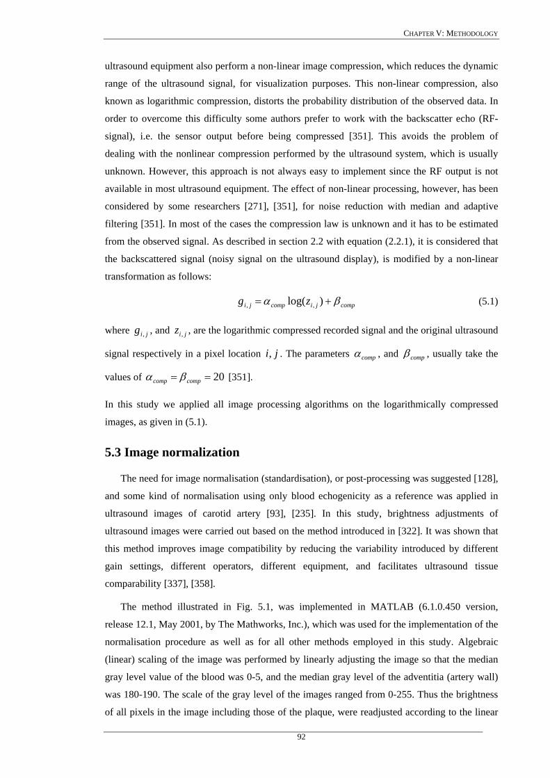
CHAPTER V: METHODOLOGY
ultrasound equipment also perform a non-linear image compression, which reduces the dynamic
range of the ultrasound signal, for visualization purposes. This non-linear compression, also
known as logarithmic compression, distorts the probability distribution of the observed data. In
order to overcome this difficulty some authors prefer to work with the backscatter echo (RF-
signal), i.e. the sensor output before being compressed [351]. This avoids the problem of
dealing with the nonlinear compression performed by the ultrasound system, which is usually
unknown. However, this approach is not always easy to implement since the RF output is not
available in most ultrasound equipment. The effect of non-linear processing, however, has been
considered by some researchers [271], [351], for noise reduction with median and adaptive
filtering [351]. In most of the cases the compression law is unknown and it has to be estimated
from the observed signal. As described in section 2.2 with equation (2.2.1), it is considered that
the backscattered signal (noisy signal on the ultrasound display), is modified by a non-linear
transformation as follows:
compjicompji zg βα += )log( ,, (5.1)
where , and , are the logarithmic compressed recorded signal and the original ultrasound
signal respectively in a pixel location . The parameters
jig , jiz ,
ji, compα , and compβ , usually take the
values of 20== compcomp βα [351].
In this study we applied all image processing algorithms on the logarithmically compressed
images, as given in (5.1).
5.3 Image normalization
The need for image normalisation (standardisation), or post-processing was suggested [128],
and some kind of normalisation using only blood echogenicity as a reference was applied in
ultrasound images of carotid artery [93], [235]. In this study, brightness adjustments of
ultrasound images were carried out based on the method introduced in [322]. It was shown that
this method improves image compatibility by reducing the variability introduced by different
gain settings, different operators, different equipment, and facilitates ultrasound tissue
comparability [337], [358].
The method illustrated in Fig. 5.1, was implemented in MATLAB (6.1.0.450 version,
release 12.1, May 2001, by The Mathworks, Inc.), which was used for the implementation of the
normalisation procedure as well as for all other methods employed in this study. Algebraic
(linear) scaling of the image was performed by linearly adjusting the image so that the median
gray level value of the blood was 0-5, and the median gray level of the adventitia (artery wall)
was 180-190. The scale of the gray level of the images ranged from 0-255. Thus the brightness
of all pixels in the image including those of the plaque, were readjusted according to the linear
92

CHAPTER V: METHODOLOGY
scale defined by the two reference regions. This results in a significant improvement in the
comparability of the ultrasound tissue characteristics. It is noted that a key point to maintaining
a high reproducibility was to ensure that the ultrasound beam was at right angles to the
adventitia, adventitia was visible adjacent to the plaque and that for image normalization a
standard sample consisting of 2/4ths of the width of the brightest area of adventitia was
obtained.
(a)
(b)
Fig. 5.1: Normalization of a carotid ultrasound image: two reference points are selected in order to normalize the image: (a) blood area is selected and, (b) adventitia area located over the plaque is selected.
Adventitia region (zoom in B-image) Selected blood area region
Final normalised image
93
CHAPTER V: METHODOLOGY
5.4 Generation of an artificial carotid image
In order to evaluate despeckle filtering, an artificial carotid image was generated. Despeckle
filtering was evaluated visually by two experts (cardiovascular surgeon, neurovascular
specialist), on the artificial carotid image corrupted by speckle noise. The artificial image
(shown in Fig. 6.3a), has a resolution of 150x150 pixels, and was generated with gray level
values of the bottom, strip, middle and upper segments of 182, 250, 102, and 158 respectively.
This image was corrupted by speckle noise, which was generated using the equation,
, where , and , are the noisy and the original images respectively,
and , a uniformly distributed random noise with mean 0 and a variance .
jijijiji fnfg ,,,, += jig , jif ,
jin , 07.02 =nσ
5.5 Image quality of two ultrasound scanners
For evaluating the image quality of the two ultrasound scanners used in this work (ATL
HDI-3000, and ATL HDI-5000), visual perception evaluation (see Chapter 5.6.1), image quality
evaluation metrics (see Chapter 4.3) and texture measures (see Chapter 4.4) were used. The
evaluation was carried out on the original (NF), normalized (N), despeckled (DS), and
normalized despeckled (NDS) images.
5.6 Despeckle filtering
In order to accurately locate structure boundaries, quantify morphology, and better visualize
the position of structures, it is necessary to pre-process the ultrasound images in a way that
suppresses the speckle noise while retaining the salient tissue boundaries in the image. Many
researchers refer to speckle as the major difficulty in analyzing and segmenting ultrasound
images [345], [348], [351].
In this work, we investigated the following despeckle filters which were presented in
Chapter 2:
• First order statistics filters- lsmv, and wiener
• Homogeneous mask areas filter-lsminsc
• Median filtering-median
• Linear scaling filtering-ls
• Maximum homogeneity filter- homog
• Geometric filtering-gf4d
• Homomorphic filtering-homo
94
CHAPTER V: METHODOLOGY
• Anisotropic diffusion-ad
• Coherence linear anisotropic diffusion-nldif
• Wavelet filtering-waveltc
In the following subsections, the visual perception evaluation, texture analysis and image
quality evaluation metrics used for evaluating the performance of despeckle filtering are
presented.
5.6.1 Visual perception evaluation
As explained in Chapter 4, visual evaluation can be broadly categorized as the ability of a
person to extract information from within an ultrasound image and to provide anatomical
information. The visual evaluation varies of course from expert to expert and is subject to the
expert’s variability [329], which may be described by the ROC curves [329], [363]. The visual
perception evaluation, in our study, was carried out according to the ITU-R recommendations,
with the DSCQS procedure [316], explained in Chapter 4.2 of this dissertation. We will
introduce in this section the procedure followed by the experts to evaluate despeckle filtering.
For the visual evaluation of the despeckle filters presented in Chapter 2, a total of 100
ultrasound images of the carotid artery, taken from 100 different patients (50 asymptomatic and
50 symptomatic) were evaluated visually by two vascular experts (a cardiovascular surgeon, and
a neurovascular expert) before and after despeckle filtering in order to assess the performance of
the filters. These 100 images were selected from the 440 image dataset using visual perception
as a criteria. A graphical user interface was developed in MATLAB as shown in Fig. 5.2 and
was used by the two experts for the visual perception evaluation. For each case, the original and
the despeckled images (despeckled with filters lsmv, lsminsc, median, wiener, ls, homog, gf4d,
homo, ad, nldif, and waveltc), were presented without labelling at random to the two experts.
The two experts evaluated the area around the distal common carotid, between 2-3 cm
before the bifurcation and the bifurcation. Furthermore, the experts were examining the image
in the lumen area, in order to identify the existence of a plaque or not, which significantly
reduces blood flow, and if the borders and the texture of the plaque were better visible after
despeckle filtering. They were examining initially the adventitial layer at the near wall of the
carotid artery, by trying to locate visually the vessel walls with the surrounding tissues. They
were then examining the far wall of the carotid artery in order to locate and visually measure the
IMT of the carotid artery, which may serve as an indicator of cardiovascular disease. To further
assess the intra-observer variability, the two experts, evaluated the same set of images,
approximately one year after the initial evaluation, as explained in Chapter 4.2.
95
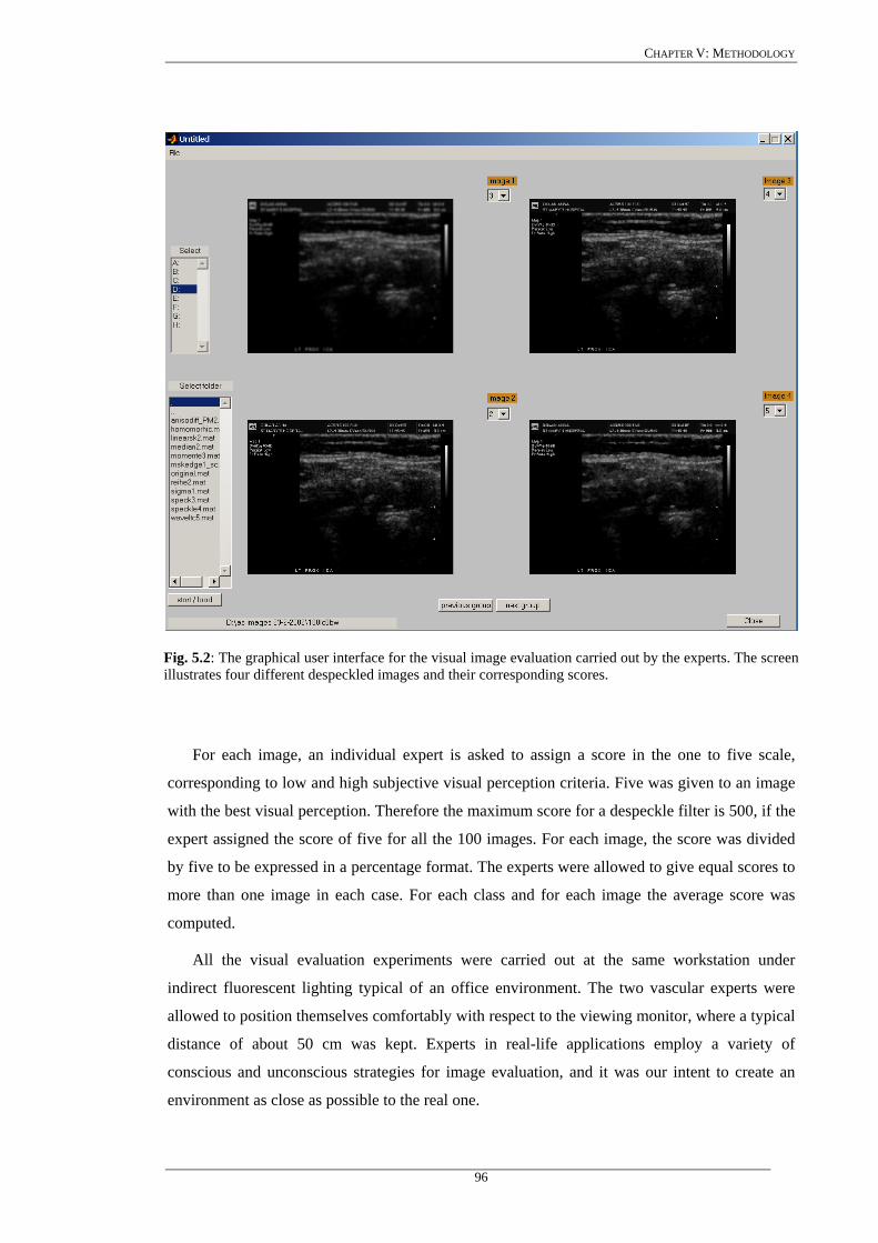
CHAPTER V: METHODOLOGY
Fig. 5.2: The graphical user interface for the visual image evaluation carried out by the experts. The screen illustrates four different despeckled images and their corresponding scores.
For each image, an individual expert is asked to assign a score in the one to five scale,
corresponding to low and high subjective visual perception criteria. Five was given to an image
with the best visual perception. Therefore the maximum score for a despeckle filter is 500, if the
expert assigned the score of five for all the 100 images. For each image, the score was divided
by five to be expressed in a percentage format. The experts were allowed to give equal scores to
more than one image in each case. For each class and for each image the average score was
computed.
All the visual evaluation experiments were carried out at the same workstation under
indirect fluorescent lighting typical of an office environment. The two vascular experts were
allowed to position themselves comfortably with respect to the viewing monitor, where a typical
distance of about 50 cm was kept. Experts in real-life applications employ a variety of
conscious and unconscious strategies for image evaluation, and it was our intent to create an
environment as close as possible to the real one.
96
CHAPTER V: METHODOLOGY
5.6.2 Texture analysis
Texture contains important information, which is used by humans for the interpretation and
the analysis of many types of images. Texture also provides useful information for the
characterization of atherosclerotic plaque [10], [127]. It is especially useful for the analysis of
natural scenes since they mostly consist of textured surfaces. Texture refers to the spatial
interrelationships and arrangement of the basic elements of an image [214]. Visually, these
spatial interrelationships and arrangements of the image pixels are seen as variations in the
intensity patterns or gray tones. Therefore, texture features have to be derived from the gray
tones of the image. Although it is easy for humans to recognize texture, it is quite a difficult task
to be defined, and subsequently to be interpreted by digital computers.
A total of 55 different texture features, introduced in Chapter 4.4 and further described in
the Appendix III, plus the speckle index (4.9), C, and the contrast-to-speckle ratio (4.10), CSR,
were extracted from the 220 asymptomatic and 220 symptomatic, original and despeckled
images.
In order to identify the most discriminant texture features, separating asymptomatic and
symptomatic ultrasound images, before and after despeckle filtering, the distance measure
(4.11), and a distance score were computed (4.14), for each feature. The most discriminant
features are the ones with the highest distance values [10]. It should be noted that for the
statistical features, second, and fourth moment, a decreasing distance shows improvement,
whereas for all other features a larger feature distance shows improvement.
The Wilcoxon matched-pairs signed rank sum test, described in Chapter 4.4.2, was used in
order to detect if for each texture feature, a significant (S) difference or not (NS), exists between
the original and the despeckled images at p<0.05. The test was applied on all the 220
asymptomatic and 220 symptomatic, original and despeckled images of the carotid artery.
The statistical k-nearest-neighbour (kNN) classifier using the Euclidean distance with k=7,
as described in Chapter 4.4.3, was also used to classify a plaque, before and after despeckle
filtering, as asymptomatic or symptomatic [10]. The leave-one-out method was used for
evaluating the performance of the classifier, where each case is evaluated in relation to the rest
of the cases. This procedure is characterized by no bias concerning the possible training and
evaluation bootstrap sets. The kNN classifier was chosen because it is simple to implement and
computationally very efficient. This is highly desired due to the many feature sets and filters
tested [211].
5.6.3 Image quality evaluation metrics
In order to evaluate differences between the original and the despeckled images, the image
quality evaluation metrics proposed in Chapter 4.3 were also used. These quality evaluation
97

CHAPTER V: METHODOLOGY
metrics MSE, RMSE, M3, M4, GAE, SNR, PSNR, Q, and SSIN, were computed for the 220
asymptomatic and 220 symptomatic ultrasound images of the carotid artery. It is noted that for
this evaluation, the image quality evaluation metrics were not divided by the low pass filtered
image (see Chapter 4.3). jilpg ,
5.7 IMT segmentation
In this section IMT manual and snakes segmentation based measurements are presented.
The IMT snakes segmentation measurements were performed in the CCA (see Fig. 1.5).
Measurements on the near wall typically suffer from lower image quality caused by overlap of
echo pulses, they are less accurate, and therefore less reproducible than those taken from the far
wall [313], [322]. This is because the adventitia is more echogenic than the blood and bright
echoes produced by the adventitia of the near wall can “spill” into the adjacent blood. Thus,
echoes from the blood are lost. This effect is far less apparent on the far wall where the media
and media-adventitia interface are closer to the probe than the adventitia. Therefore a far wall
measurement is utilized most frequently. The IMT was defined as the distance between the
leading edge of the lumen-intima interface and the leading edge of the medial-adventitia
interface (see Fig. 3.1, interfaces Z5-Z7).
5.7.1 Manual measurements and visual perception evaluation
Using a system developed in MATLAB, the two experts manually outlined the IMT
according to a specific protocol which will be described below. Figure 5.3 demonstrates the
manual IMT segmentation software. The software provided an easy to use user interface for
segmenting the vessel wall and the lumen directly from the acquired ultrasound images.
Although the power Doppler (blood flow image) was found to be useful for locating the
lumen, only the B-mode image was used when delineating the wall and the lumen boundaries in
order to eliminate errors due to color artifacts and reverberations occurring from the blood flow
image [208], [238], [322]. For the purpose of this study the vessel wall and lumen are defined
as follows:
a) The lumen is the boundary enclosing the interior region of the vessel through which
blood flows (see Fig. 3.1, interface Z4).
b) The lumen appears as a dark region in a B-mode ultrasound image (see Fig. 3.1,
region between interfaces Z3-Z5).
c) The vessel wall is the boundary separating the intima-blood interface (see Fig. 3.1
interface Z5).
98
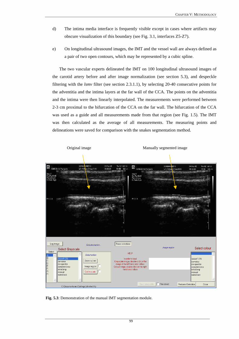
CHAPTER V: METHODOLOGY
d) The intima media interface is frequently visible except in cases where artifacts may
obscure visualization of this boundary (see Fig. 3.1, interfaces Z5-Z7).
e) On longitudinal ultrasound images, the IMT and the vessel wall are always defined as
a pair of two open contours, which may be represented by a cubic spline.
The two vascular experts delineated the IMT on 100 longitudinal ultrasound images of
the carotid artery before and after image normalization (see section 5.3), and despeckle
filtering with the lsmv filter (see section 2.3.1.1), by selecting 20-40 consecutive points for
the adventitia and the intima layers at the far wall of the CCA. The points on the adventitia
and the intima were then linearly interpolated. The measurements were performed between
2-3 cm proximal to the bifurcation of the CCA on the far wall. The bifurcation of the CCA
was used as a guide and all measurements made from that region (see Fig. 1.5). The IMT
was then calculated as the average of all measurements. The measuring points and
delineations were saved for comparison with the snakes segmentation method.
Fig. 5.3: Demonstration of the manual IMT segmentation module.
Original image Manually segmented image
99
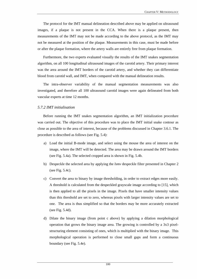
CHAPTER V: METHODOLOGY
The protocol for the IMT manual delineation described above may be applied on ultrasound
images, if a plaque is not present in the CCA. When there is a plaque present, then
measurements of the IMT may not be made according to the above protocol, as the IMT may
not be measured at the position of the plaque. Measurements in this case, must be made before
or after the plaque formation, where the artery walls are entirely free from plaque formation.
Furthermore, the two experts evaluated visually the results of the IMT snakes segmentation
algorithm, on all 100 longitudinal ultrasound images of the carotid artery. Their primary interest
was the area around the IMT borders of the carotid artery, and whether they can differentiate
blood from carotid wall, and IMT, when compared with the manual delineation results.
The intra-observer variability of the manual segmentation measurements was also
investigated, and therefore all 100 ultrasound carotid images were again delineated from both
vascular experts at time 12 months.
5.7.2 IMT initialisation
Before running the IMT snakes segmentation algorithm, an IMT initialization procedure
was carried out. The objective of this procedure was to place the IMT initial snake contour as
close as possible to the area of interest, because of the problems discussed in Chapter 3.6.1. The
procedure is described as follows (see Fig. 5.4):
a) Load the initial B-mode image, and select using the mouse the area of interest on the
image, where the IMT will be detected. The area may be drawn around the IMT borders
(see Fig. 5.4a). The selected cropped area is shown in Fig. 5.4b.
b) Despeckle the selected area by applying the lsmv despeckle filter presented in Chapter 2
(see Fig. 5.4c).
c) Convert the area to binary by image thresholding, in order to extract edges more easily.
A threshold is calculated from the despeckled grayscale image according to [15], which
is then applied to all the pixels in the image. Pixels that have smaller intensity values
than this threshold are set to zero, whereas pixels with larger intensity values are set to
one. The area is thus simplified so that the borders may be more accurately extracted
(see Fig. 5.4d).
d) Dilate the binary image (from point c above) by applying a dilation morphological
operation that grows the binary image area. The growing is controlled by a 3x3 pixel-
structuring element consisting of ones, which is multiplied with the binary image. This
morphological operation is performed to close small gaps and form a continuous
boundary (see Fig. 5.4e).
100
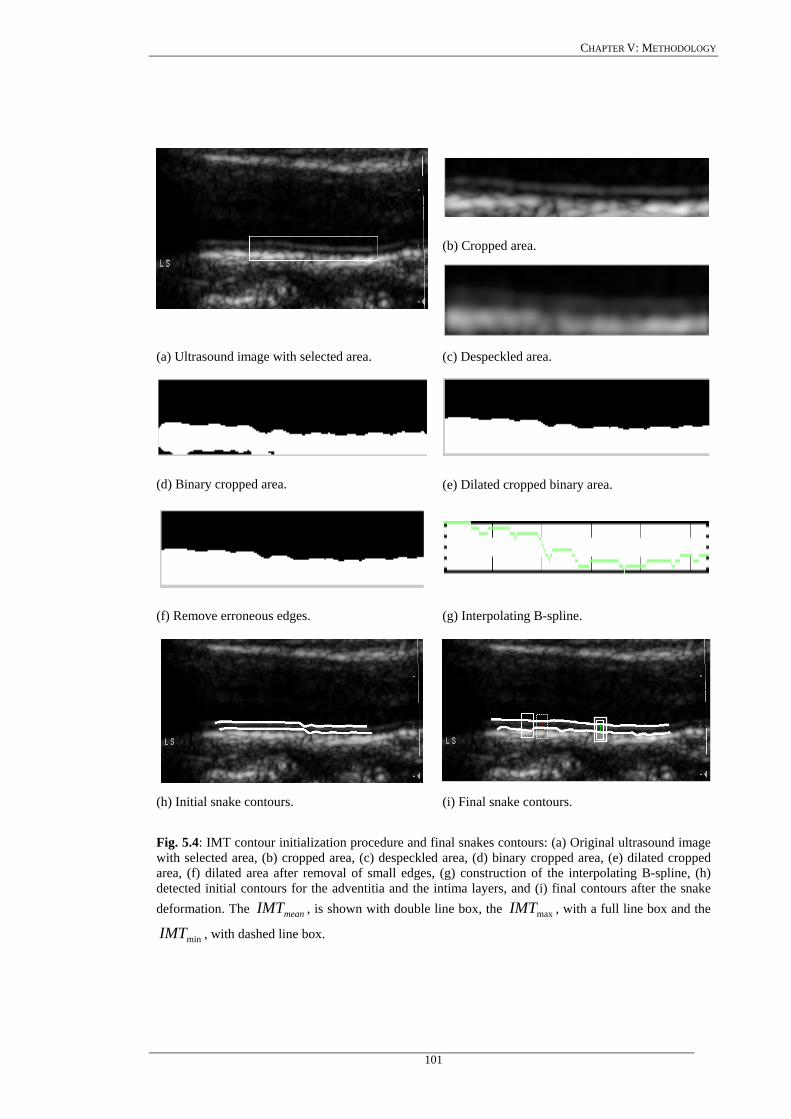
CHAPTER V: METHODOLOGY
(b) Cropped area.
(a) Ultrasound image with selected area. (c) Despeckled area.
(d) Binary cropped area. (e) Dilated cropped binary area.
(f) Remove erroneous edges. (g) Interpolating B-spline.
(h) Initial snake contours. (i) Final snake contours.
Fig. 5.4: IMT contour initialization procedure and final snakes contours: (a) Original ultrasound image with selected area, (b) cropped area, (c) despeckled area, (d) binary cropped area, (e) dilated cropped area, (f) dilated area after removal of small edges, (g) construction of the interpolating B-spline, (h) detected initial contours for the adventitia and the intima layers, and (i) final contours after the snake deformation. The , is shown with double line box, the , with a full line box and the
, with dashed line box. meanIMT maxIMT
minIMT
101
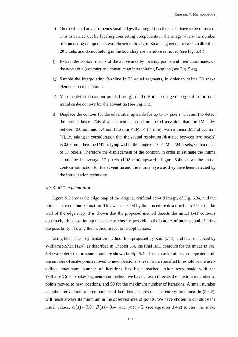
CHAPTER V: METHODOLOGY
e) On the dilated area erroneous small edges that might trap the snake have to be removed.
This is carried out by labeling connecting components in the image where the number
of connecting components was chosen to be eight. Small segments that are smaller than
20 pixels, and do not belong in the boundary are therefore removed (see Fig. 5.4f).
f) Extract the contour matrix of the above area by locating points and their coordinates on
the adventitia (contour) and construct an interpolating B-spline (see Fig. 5.4g).
g) Sample the interpolating B-spline in 30 equal segments, in order to define 30 snake
elements on the contour.
h) Map the detected contour points from g), on the B-mode image of Fig. 5a) to form the
initial snake contour for the adventitia (see Fig. 5h).
i) Displace the contour for the adventitia, upwards for up to 17 pixels (1.02mm) to detect
the intima layer. This displacement is based on the observation that the IMT lies
between 0.6 mm and 1.4 mm (0.6 mm < IMT< 1.4 mm), with a mean IMT of 1.0 mm
[7]. By taking in consideration that the spatial resolution (distance between two pixels)
is 0.06 mm, then the IMT is lying within the range of 10 < IMT <24 pixels, with a mean
of 17 pixels. Therefore the displacement of the contour, in order to estimate the intima
should be in average 17 pixels (1.02 mm) upwards. Figure 5.4h shows the initial
contour estimation for the adventitia and the intima layers as they have been detected by
the initialization technique.
5.7.3 IMT segmentation
Figure 5.5 shows the edge map of the original artificial carotid image, of Fig. 6.3a, and the
initial snake contour estimation. This was detected by the procedure described in 5.7.2 at the far
wall of the edge map. It is shown that the proposed method detects the initial IMT contours
accurately, thus positioning the snake as close as possible to the borders of interest, and offering
the possibility of using the method in real time applications.
Using the snakes segmentation method, first proposed by Kass [243], and later enhanced by
Williams&Shah [124], as described in Chapter 3.4, the final IMT contours for the image in Fig.
5.4a were detected, measured and are shown in Fig. 5.4i. The snake iterations are repeated until
the number of snake points moved to new locations is less than a specified threshold or the user-
defined maximum number of iterations has been reached. After tests made with the
Williams&Shah snakes segmentation method, we have chosen three as the maximum number of
points moved to new locations, and 50 for the maximum number of iterations. A small number
of points moved and a large number of iterations ensures that the energy functional in (3.4.2),
will reach always its minimum in the observed area of points. We have chosen in our study the
initial values, 6.0)( =sα , 4.0)( =sβ , and 2)( =sγ (see equation 3.4.2) to start the snake
102

CHAPTER V: METHODOLOGY
deformation which is consistent with other studies [241], [252], [260]. Figure 5.6 shows the
module developed using the MATLAB software for the IMT segmentation in ultrasound images
of the carotid artery.
After both final snake contours have been extracted (see Fig. 5.4i), the distance lumen-
intima interface to the media-adventitia interface is measured between pixel pairs. This distance
is calculated at all points along the arterial segment of interest and then averaged to obtain the
mean IMT ( ). Also the maximum ( ), minimum ( ), and median
( ) IMT values, are calculated, displayed, and plotted on the B-mode image. Figure
5.4i shows the detected , , and values with a double line box, full line
box, and a dashed line box respectively.
meanIMT maxIMT minIMT
medianIMT
meanIMT maxIMT minIMT
Fig. 5.5: Edge map of an artificial carotid image of the original image in Fig. 6.3a, and the detected initial contours for the IMT.
When segmenting the IMT, the user has to decide first, which layer, intima or adventitia, is
better to detect based on the images available taking into consideration the following:
a) Is there a lot of noise in the lumen near the intima?
b) Which layer, intima or adventitia, has a stronger contrast?
c) Are the edges on the image better displayed at the intima or at the adventitia
layer?
Relying on our experience after experiments carried out, and based on a number of
unpublished observations, there is a strong noise component in the lumen near the intima. On
the other hand, it seems that the adventitia has a stronger contrast. Therefore, it is better if the
IMT detection starts first from the adventitia. Prior to the segmentation, the image, or the
selected area of interest, which is the area around the IMT, is enhanced by applying the
despeckle filter lsmv (see Chapter 2.3.1.1). We can also apply normalisation to the selected area
as proposed in Chapter 5.3, by enhancing the gray level change from black to white [322].
103
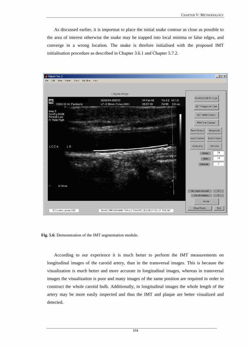
CHAPTER V: METHODOLOGY
As discussed earlier, it is importnat to place the initial snake contour as close as possible to
the area of interest otherwise the snake may be trapped into local minima or false edges, and
converge in a wrong location. The snake is threfore initialised with the proposed IMT
initialisation procedure as described in Chapter 3.6.1 and Chapter 5.7.2.
Fig. 5.6: Demonstration of the IMT segmentation module.
According to our experience it is much better to perform the IMT measurements on
longitudinal images of the carotid artery, than in the transversal images. This is because the
visualization is much better and more accurate in longitudinal images, whereas in transversal
images the visualization is poor and many images of the same position are required in order to
construct the whole carotid bulb. Additionally, in longitudinal images the whole length of the
artery may be more easily inspected and thus the IMT and plaque are better visualized and
detected.
104
CHAPTER V: METHODOLOGY
5.7.4 Univariate statistical analysis
The Williams&Shah IMT snakes segmentation method was applied on 100 longitudinal
ultrasound images of the carotid artery. In order to investigate how the results of the snakes
segmentation method, differs from the manual delineation results, we used the following
evaluation metrics.
We computed the parameters, , , and , as well as the
inter-observer error [265]:
meanIMT minIMT maxIMT medianIMT
2/IMTse σ= . (5.2)
where IMTσ is the variance of all IMT measurements. We also calculated the coefficient of
variation, , which describes the difference as a percentage of the pooled mean value,
[131], [265]:
%CV
meanIMT
100%meanIMT
seCV = . (5.3)
The Wilcoxon matched-pairs signed rank sum test was also used in order to identify if for
each measurement a significant (S) difference or not (NS) exists between the snakes and the
manual segmented boundaries, at 05.0<p .
Further a variation of the Hausdorff distance, HD , [265], between two curves was
calculated. It reflects the maximum mismatch between the manual and the snakes segmented
areas, and is calculated as:
SegmentedSnakeManualHD _−= . (5.4)
where small values for the HD are favourable.
Also the Pearson correlation test was used, at a significance level of 0.05, which returns the
Pearson product moment correlation coefficient, , that ranges from –1.0 to 1.0 inclusive
and reflects the extent of a linear relationship between two data sets [265].
pearsonr
The , between the snakes segmented and the manually segmented boundaries was also
calculated, which estimates the minimum average distance squared [131], between the two
curves. Therefore small values for are required.
MSE
MSE
The strength of the relationship between the snakes segmented and the manually segmented
methods is indicated by the correlation:
105
CHAPTER V: METHODOLOGY
am
amam
Covc
σσ,
, = , (5.5)
where , is the covariance between the snakes (a) and the manual (m) measurements and, amCov ,
mσ , aσ , are the standard deviations of the two measurements respectively [269]. Further, the
correlation coefficient, corelρ , was investigated to determine the relationship between the
measurements at a significance level of 0.05 (i.e. for 100 subjects correlation values above
0.1654 are significant).
These statistical metrics have been computed for the Williams&Shah snakes segmentation
measurements for the cases, no filtering (NF), despeckled (DS), normalized (N), normalized
despeckled (NDS), and for the manual segmentation measurements, for the cases, manual (M),
and manual normalized (MN) from both experts, respectively. Additionally, in order to assess
the intra-observer variability between the two experts, the manual measurements on original
(M), and normalized (MN) images were repeated from both experts, one year after the first
measurements.
In order to assess the normality of the distributions, histograms for all the values
were computed. Specifically, the histograms for the 100-ultrasound images of the carotid artery
were plotted, for the snakes segmentation cases NF, DS, N, NDS, and for the manual
segmentation cases M, and MN, from both experts. If the histogram of a distribution is skewed
or has very long tails, then the assumption of normality may not be valid [264].
meanIMT
Furthermore, box plots (Whisker diagrams) were computed for the snakes segmentation
cases NF, DS, N, NDS, and the manual segmentation cases M, and MN from both experts. The
box plots, demonstrate the dispersion or spread of the distribution for the values, for
all the 100-ultrasound images of the carotid artery. A box plot diagram provides a simple
graphical summary of the set of data. It shows a measure of central location (the median), two
measures of dispersion (the range and inter-quartile range), the skewness (from the orientation
of the median relative to the quartiles) and potential outliers (marked individually). Box plots
are especially useful when comparing two or more sets of data and can be used to indicate the
degree of symmetry in a distribution.
meanIMT
Bland-Altman plots [264] were also used to further evaluate the agreement between the
Williams&Shah snakes segmentation and the manual segmentation method. The plots were
investigated for the snakes segmentation cases, NF, DS, N, NDS, and for the manual
segmentation cases M, and MN, from both experts. By using Bland-Altman plots, the
distributions of the differences between all different cases were computed.
106
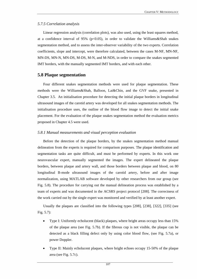
CHAPTER V: METHODOLOGY
5.7.5 Correlation analysis
Linear regression analysis (correlation plots), was also used, using the least squares method,
at a confidence interval of 95% (p<0.05), in order to validate the Williams&Shah snakes
segmentation method, and to assess the inter-observer variability of the two experts. Correlation
coefficients, slope and intercept, were therefore calculated, between the cases M-NF, MN-NF,
MN-DS, MN-N, MN-DS, M-DS, M-N, and M-NDS, in order to compare the snakes segmented
IMT borders, with the manually segmented IMT borders, and with each other.
5.8 Plaque segmentation
Four different snakes segmentation methods were used for plaque segmentation. These
methods were the Williams&Shah, Balloon, Lai&Chin, and the GVF snake, presented in
Chapter 3.5. An initialisation procedure for detecting the initial plaque borders in longitudinal
ultrasound images of the carotid artery was developed for all snakes segmentation methods. The
initialisation procedure uses, the outline of the blood flow image to detect the initial snake
placement. For the evaluation of the plaque snakes segmentation method the evaluation metrics
proposed in Chapter 4.5 were used.
5.8.1 Manual measurements and visual perception evaluation
Before the detection of the plaque borders, by the snakes segmentation method manual
delineation from the experts is required for comparison purposes. The plaque identification and
segmentation tasks are quite difficult, and must be performed by experts. In this work one
neurovascular expert, manually segmented the images. The expert delineated the plaque
borders, between plaque and artery wall, and those borders between plaque and blood, on 80
longitudinal B-mode ultrasound images of the carotid artery, before and after image
normalization, using MATLAB software developed by other researchers from our group (see
Fig. 5.8). The procedure for carrying out the manual delineation process was established by a
team of experts and was documented in the ACSRS project protocol [208]. The correctness of
the work carried out by the single expert was monitored and verified by at least another expert.
Usually the plaques are classified into the following types [208], [238], [322], [335] (see
Fig. 5.7):
• Type I: Uniformly echolucent (black) plaques, where bright areas occupy less than 15%
of the plaque area (see Fig. 5.7b). If the fibrous cup is not visible, the plaque can be
detected as a black filling defect only by using color blood flow, (see Fig. 5.7a), or
power Doppler.
• Type II: Mainly echolucent plaques, where bright echoes occupy 15-50% of the plaque
area (see Fig. 5.7c).
107
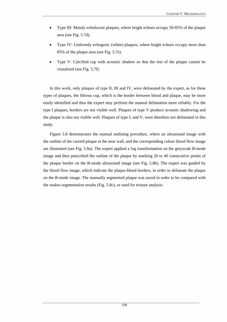
CHAPTER V: METHODOLOGY
• Type III: Mainly echolucent plaques, where bright echoes occupy 50-85% of the plaque
area (see Fig. 5.7d).
• Type IV: Uniformly echogenic (white) plaques, where bright echoes occupy more than
85% of the plaque area (see Fig. 5.7e).
• Type V: Calcified cup with acoustic shadow so that the rest of the plaque cannot be
visualized (see Fig. 5.7f).
In this work, only plaques of type II, III and IV, were delineated by the expert, as for these
types of plaques, the fibrous cup, which is the border between blood and plaque, may be more
easily identified and thus the expert may perform the manual delineation more reliably. For the
type I plaques, borders are not visible well. Plaques of type V produce acoustic shadowing and
the plaque is also not visible well. Plaques of type I, and V, were therefore not delineated in this
study.
Figure 5.8 demonstrates the manual outlining procedure, where an ultrasound image with
the outline of the carotid plaque at the near wall, and the corresponding colour blood flow image
are illustrated (see Fig. 5.8a). The expert applied a log transformation on the greyscale B-mode
image and then prescribed the outline of the plaque by marking 20 to 40 consecutive points of
the plaque border on the B-mode ultrasound image (see Fig. 5.8b). The expert was guided by
the blood flow image, which indicate the plaque-blood borders, in order to delineate the plaque
on the B-mode image. The manually segmented plaque was saved in order to be compared with
the snakes segmentation results (Fig. 5.8c), or used for texture analysis.
108
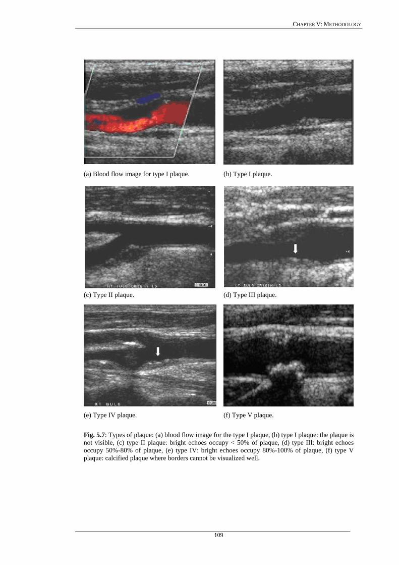
CHAPTER V: METHODOLOGY
(a) Blood flow image for type I plaque. (b) Type I plaque.
(c) Type II plaque. (d) Type III plaque.
(e) Type IV plaque. (f) Type V plaque.
Fig. 5.7: Types of plaque: (a) blood flow image for the type I plaque, (b) type I plaque: the plaque is not visible, (c) type II plaque: bright echoes occupy < 50% of plaque, (d) type III: bright echoes occupy 50%-80% of plaque, (e) type IV: bright echoes occupy 80%-100% of plaque, (f) type V plaque: calcified plaque where borders cannot be visualized well.
109
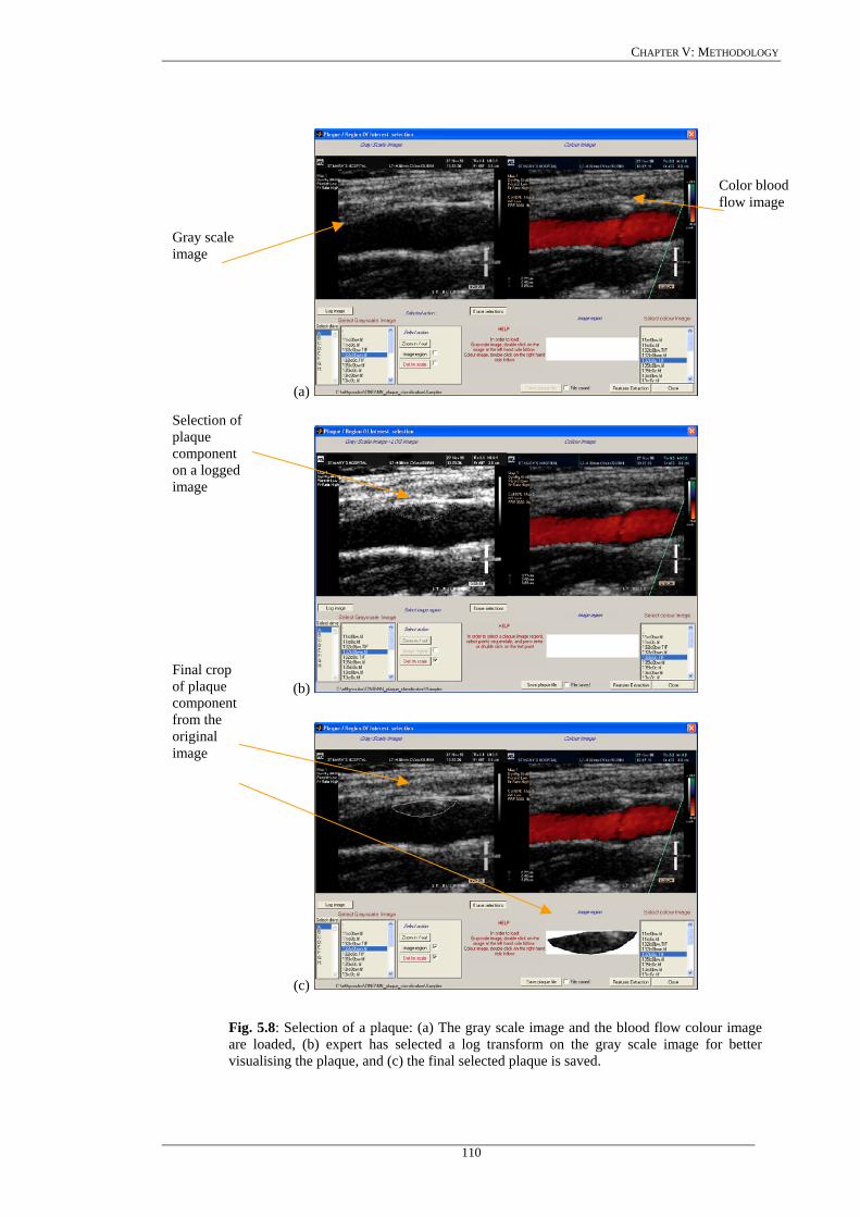
CHAPTER V: METHODOLOGY
Color bflow image
lood
(a)
(b)
(c)
Fig. 5.8: Selection of a plaque: (a) The gray scale image and the blood flow colour image are loaded, (b) expert has selected a log transform on the gray scale image for better visualising the plaque, and (c) the final selected plaque is saved.
Gray scale image Selection of plaque component on a logged image Final crop of plaque component from the original image
110

CHAPTER V: METHODOLOGY
5.8.2 Plaque initialisation using the blood flow image
In most of the cases a plaque is visualised in a B-mode longitudinal ultrasound image and its
size confirmed in transverse section. However, uniformly echolucent plaques are not obvious on
B-mode, and colour flow imaging is needed. These echolucent plaques, are seen as black filling
deffects. PW Doppler is used to measure velocity in order to grade the degree of stenosis. In this
work we have used the blood flow image, in order to extract the initial snake contour estimation
for the plaque borders in the carotid artery. The limitations of this approach, i.e. using the blood
flow image to locate the blood borders are the following:
a) The colour flow sometimes overlaps with areas of the tissue wall or a plaque, and
b) The colour does not always fill up places where the blood has a low speed.
In this subsection we describe the plaque snake contour initialsation procedure, carried out
using both the blood flow and the B-mode images. This procedure may be described as follows
(see Fig. 5.9):
a) Cross correlate the B-mode image (Fig. 5.9a) with the blood flow image (Fig. 5.9b)
and extract the borders of the blood flow area.
b) Dilate the extracted blood flow edge image, to eliminate small gaps and remove small
undesired regions.
c) From the dilated edge blood flow image, detect the blood flow edge contour (see Fig.
5.9c). Mark a region of interest on the edge contour (a task carried out by the expert,
illustrated by a rectangle in Fig. 5.9c) where the lower or upper boundary of plaque is
covered. This is used as an initial snake contour.
d) Sample the initial snake contour at 20 to 40 consecutive points to construct an
interpolating B-spline.
e) Connect the first and the last snake points on the initial contour to form a close
contour.
f) Despeckle the B-mode image by the lsmv filter described in Chapter 2.3.1.1.
g) Map the initial plaque contour on the B-mode image (see Fig. 5.9d).
h) Deform the initial contour by the snake to accurately locate the plaque-blood borders,
and
i) Save the final plaque contour and display it on the B-mode image (see Fig. 5.9e).
111
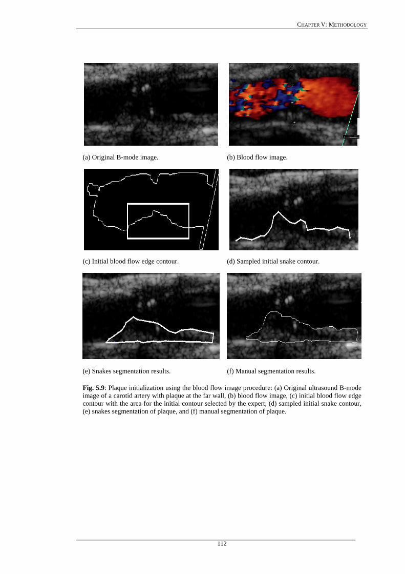
CHAPTER V: METHODOLOGY
(a) Original B-mode image. (b) Blood flow image.
(c) Initial blood flow edge contour. (d) Sampled initial snake contour.
(e) Snakes segmentation results. (f) Manual segmentation results.
Fig. 5.9: Plaque initialization using the blood flow image procedure: (a) Original ultrasound B-mode image of a carotid artery with plaque at the far wall, (b) blood flow image, (c) initial blood flow edge contour with the area for the initial contour selected by the expert, (d) sampled initial snake contour, (e) snakes segmentation of plaque, and (f) manual segmentation of plaque.
112
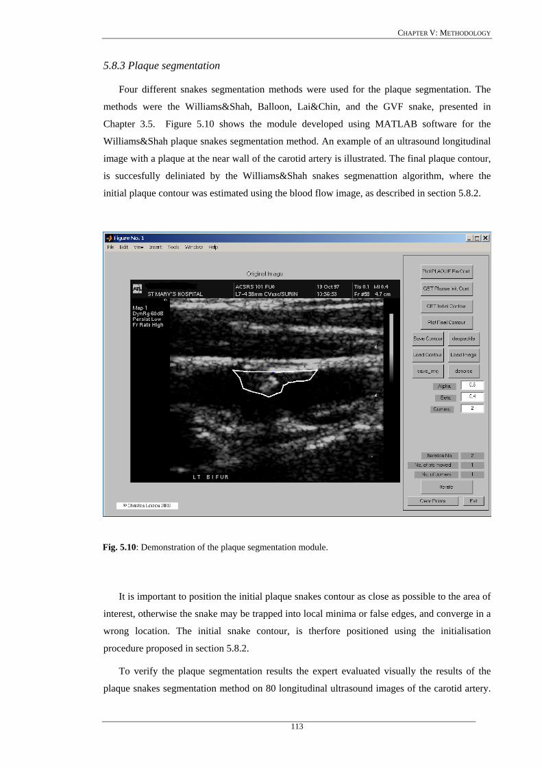
CHAPTER V: METHODOLOGY
5.8.3 Plaque segmentation
Four different snakes segmentation methods were used for the plaque segmentation. The
methods were the Williams&Shah, Balloon, Lai&Chin, and the GVF snake, presented in
Chapter 3.5. Figure 5.10 shows the module developed using MATLAB software for the
Williams&Shah plaque snakes segmentation method. An example of an ultrasound longitudinal
image with a plaque at the near wall of the carotid artery is illustrated. The final plaque contour,
is succesfully deliniated by the Williams&Shah snakes segmenattion algorithm, where the
initial plaque contour was estimated using the blood flow image, as described in section 5.8.2.
Fig. 5.10: Demonstration of the plaque segmentation module.
It is important to position the initial plaque snakes contour as close as possible to the area of
interest, otherwise the snake may be trapped into local minima or false edges, and converge in a
wrong location. The initial snake contour, is therfore positioned using the initialisation
procedure proposed in section 5.8.2.
To verify the plaque segmentation results the expert evaluated visually the results of the
plaque snakes segmentation method on 80 longitudinal ultrasound images of the carotid artery.
113
CHAPTER V: METHODOLOGY
The primary interest of the expert was to check if the plaque borders and the outline of the
plaque were detected correctly by the snakes segmentation methods.
The four different snakes segmentation methods implemented were, the Balloon snake
[333], the snake of Lai&Chin [248], and the GVF snake [116], as presented in Chapters 3.5.1-
3.5.3, which were compared with the Williams&Shah (see Chapter 3.4) snakes segmentation
method.
All four different plaque snakes segmentation methods were evaluated on 80 symptomatic
B-mode and blood flow (PW Doppler) longitudinal ultrasound images of the CCA, representing
different types of atherosclerotic plaque formation with irregular geometry typically found in
this blood vessel.
The parameter values for the four different snakes segmentation methods, were the same in
all experiments, and they were chosen for the Williams&Shah snake to be equal to 6.0=α ,
4.0=β , 2=γ , the regularisation parameter, πλ , for the Lai&Chin snake, was variable and
was calculated according to (3.5.5), and (3.5.6), and the elasticity, rigidity and the regularisation
parameters for the GVF snake was, 05.0=GVFα , 0=GVFβ , 2.0=GVFµ , which are consistent
with other studies [53], [241], [252], [260].
The four different plaque snakes segmentation methods were evaluated in three longitudinal
ultrasound plaque images of the carotid artery bifurcation by calculating the number of the
snake iterations, and the computational time needed for the snake to converge in its final
position. The computational efficiency of the algorithms was tested by direct comparisons of
iterations and computational time between the four different plaque snakes segmentation
algorithms.
To furthermore demonstrate the working principle of the four plaque snakes segmentation
methods, the total snake energy (3.4.2), , the continuity energy, , the
curvature energy, , and the image energy, , were plotted over the number of
iterations. Furthermore, the snake parameters,
)(vEsnake )(vEcont
)(vEcurv )(vEimage
α , and β , (see 3.4.2) for the Lai&Chin snakes
segmentation method were plotted over the number of iterations. The variability of these
parameters over the time was thus investigated.
5.8.4 ROC analysis of plaque segmenattion methods
In order to evaluate the performance of the four plaque snakes segmentation methods, we
compared the manually segmented borders, delineated by an expert, with the snakes segmented
borders on all 80 ultrasound images. The ROC analysis was used, with the true and false
positives, and negative fractions, to assess the specificity, and sensitivity of the segmentation
114

CHAPTER V: METHODOLOGY
method, by the true-positive fraction, TPF , and false-positive fraction, FPF , detected (see
Chapter 4.5) [363]. Some additional performance metrics proposed in Chapter 4.5, such as the
sensitivity, R (4.16), the specificity, (4.17), the precision, Sp P (4.18), and (see 4.19),
which is calculated from the effectiveness measure
F
E , were also calculated for all four different
snakes segmentation methods. Box plots of TPF, TNF, FPF, FNF, KI index, and overlap index,
were plotted for all four different snakes segmentation methods.
Furthermore, ROC curves for all four different snakes segmentation methods were plotted
and compared with each other. ROC curves [363] are used as a standard analysis tool to
evaluate the sensitivity, R , (4.16), and specificity, , (4.17), of diagnostic procedures. ROC
analysis estimates a curve of the positive rate (sensitivity), versus the false positive rate (1-
specificity), which describes the inherent tradeoff sensitivity and specificity of a diagnostic
system.
Sp
115

CHAPTER VI: RESULTS
Chapter 6
Results
116

CHAPTER VI: RESULTS
CHAPTER 6: RESULTS
In this Chapter we present the image quality evaluation results of two ultrasound scanners,
the results of the despeckle filters presented in Chapter 2, the performance of the
Williams&Shah snakes segmentation technique for the IMT, presented in Chapter 3.4, as well
as the plaque segmentation results for the four different snakes segmentation techniques,
presented in Chapter 3.5, namely the Williams&Shah, Balloon, Lai&Chin, and the GVF.
Various criteria were used in order to compare the effectiveness of the despeckle filters such as:
µ , , , , SNR, C, CSR, and other image and texture metrics, as presented in Chapter
4.3 and Chapter 4.4. These metrics were applied on the original and despeckled images
respectively. For evaluating the IMT and plaque segmentation methods, the evaluation metrics
presented in Chapter 5.7.4, Chapter 5.7.5, and Chapter 4.5 were also used. Two experts
evaluated visually the despeckle filtering results. Two experts manually delineated the IMT
whereas one expert manually delineated the plaque contour.
2σ 3σ 4σ
6.1 Image quality evaluation of two ultrasound scanners
In this section, we evaluate image quality, based on MSE, RMSE, Err3, Err4, GAE, SNR,
PSNR, quality index, Q, and structural similarity index, SSIN, in ultrasound imaging of the
carotid artery. These criteria as well as statistical and texture features were computed on 80
ultrasound longitudinal images of the carotid artery bifurcation, recorded from two different
ultrasound scanners, the ATL HDI-3000, and the ATL HDI-5000, before and after despeckle
filtering, and after despeckle filtering and normalization. The image quality and texture
measures were presented in Chapter 4.3, and Chapter 4.4, respectively (see also Chapter 5.5).
The results of our study showed that image quality was improved after normalisation and
normalization and despeckle filtering for both scanners. This finding is also in agreement with
the visual perception evaluation carried out by the two vascular experts. Furthermore, the
ultrasound images may be better visualised with the HDI ATL-5000 scanner, after
normalisation and normalisation and despeckle filtering.
6.1.1 Visual perception
Figure 6.1 illustrates the original before filtering, NF, despeckled, DS, normalised, N, and
normalised despeckled, NDS, images for the two ultrasound image scanners. The images were
depseckled with the filter lsmv (Chapter 2.3.1.1), which was applied for four times iteratively on
the images using a 5x5 pixel window. It was shown that the images for the ATL HDI-3000
scanner have greater speckle noise compared to the ATL HDI-5000 images. Moreover the
117
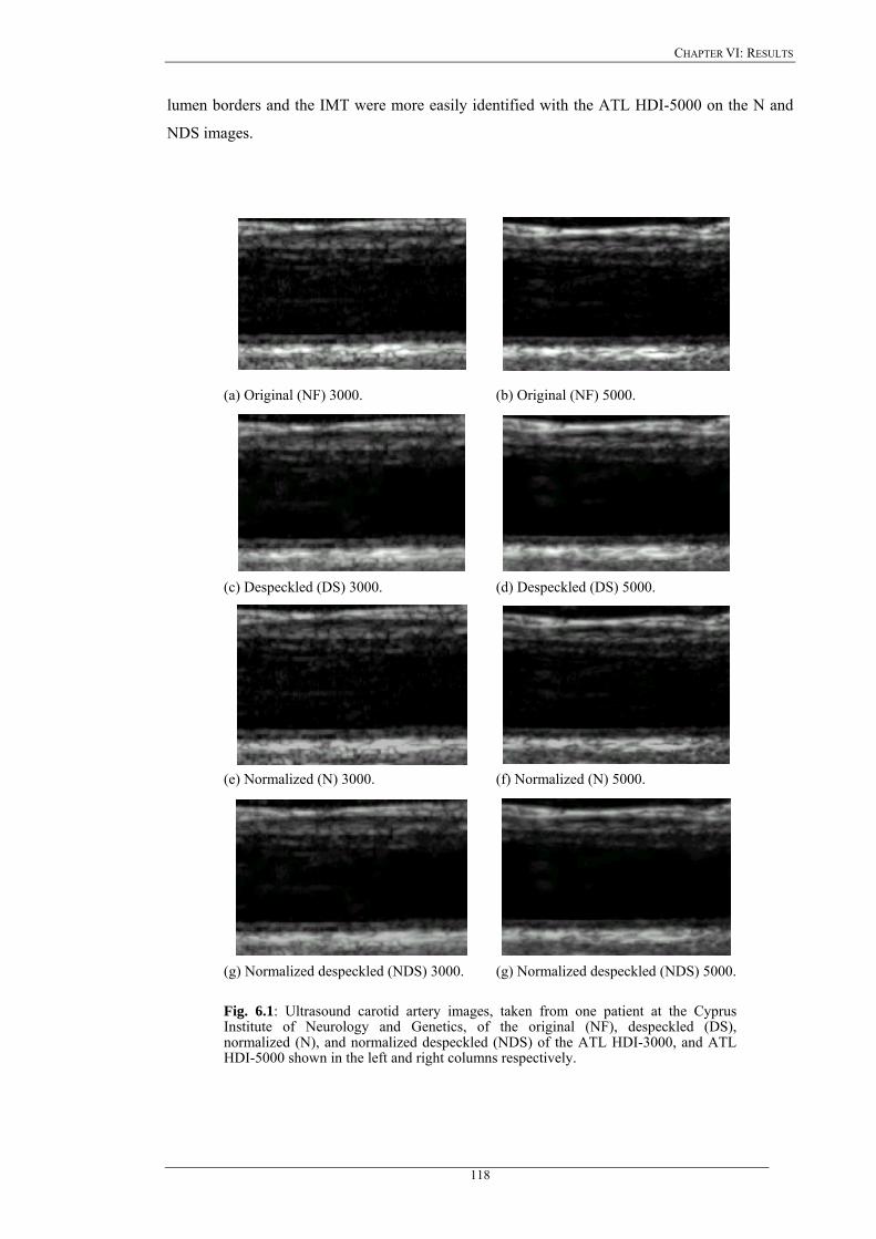
CHAPTER VI: RESULTS
lumen borders and the IMT were more easily identified with the ATL HDI-5000 on the N and
NDS images.
(a) Original (NF) 3000. (b) Original (NF) 5000.
(c) Despeckled (DS) 3000. (d) Despeckled (DS) 5000.
(e) Normalized (N) 3000. (f) Normalized (N) 5000.
(g) Normalized despeckled (NDS) 3000. (g) Normalized despeckled (NDS) 5000.
Fig. 6.1: Ultrasound carotid artery images, taken from one patient at the Cyprus Institute of Neurology and Genetics, of the original (NF), despeckled (DS), normalized (N), and normalized despeckled (NDS) of the ATL HDI-3000, and ATL HDI-5000 shown in the left and right columns respectively.
118
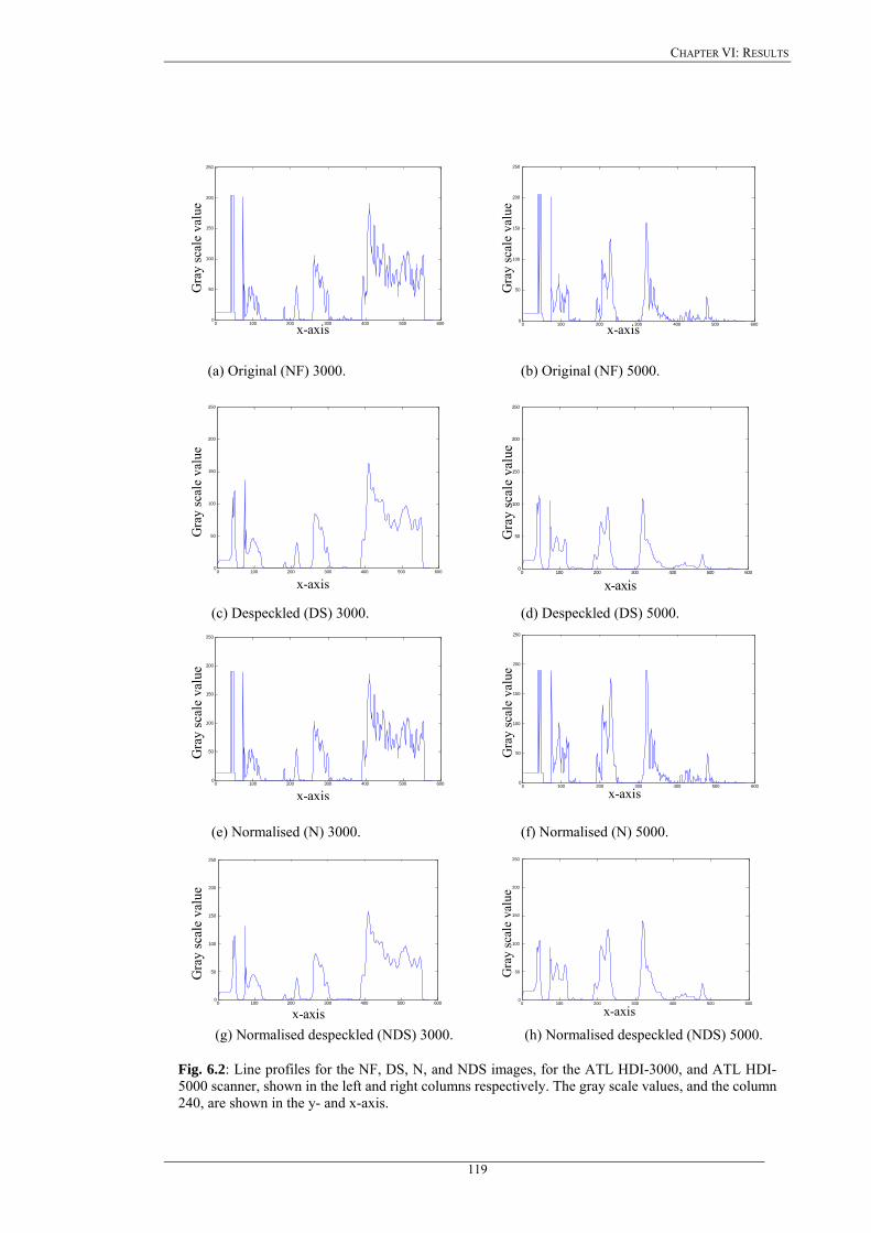
CHAPTER VI: RESULTS
0 100 200 300 400 500 6000
50
100
150
200
250
Gra
y sc
ale
valu
e
x-axis
0 100 200 300 400 500 6000
50
100
150
200
250
x-axis
Gra
y sc
ale
valu
e
(a) Original (NF) 3000. (b) Original (NF) 5000.
0 100 200 300 400 500 6000
50
100
150
200
250
x-axis
Gra
y sc
ale
valu
e
0 100 200 300 400 500 6000
50
100
150
200
250
x-axis
Gra
y sc
ale
valu
e
(c) Despeckled (DS) 3000. (d) Despeckled (DS) 5000.
0 100 200 300 400 500 6000
50 100 150 200 250
x-axis
Gra
y sc
ale
valu
e
0 100 200 300 400 500 6000
50
100
150
200
250
x-axis
Gra
y sc
ale
valu
e
(e) Normalised (N) 3000. (f) Normalised (N) 5000.
0 100 200 300 400 500 6000
50 100 150 200 250
x-axis
Gra
y sc
ale
valu
e
0 100 200 300 400 500 6000
50
100
150
200
250
x-axis
Gra
y sc
ale
valu
e
(g) Normalised despeckled (NDS) 3000. (h) Normalised despeckled (NDS) 5000.
Fig. 6.2: Line profiles for the NF, DS, N, and NDS images, for the ATL HDI-3000, and ATL HDI-5000 scanner, shown in the left and right columns respectively. The gray scale values, and the column 240, are shown in the y- and x-axis.
119
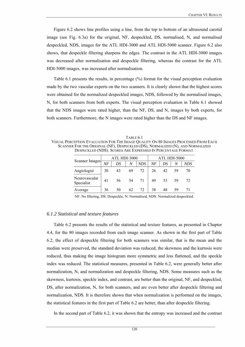
CHAPTER VI: RESULTS
Figure 6.2 shows line profiles using a line, from the top to bottom of an ultrasound carotid
image (see Fig. 6.3a) for the original, NF, despeckled, DS, normalised, N, and normalised
despeckled, NDS, images for the ATL HDI-3000 and ATL HDI-5000 scanner. Figure 6.2 also
shows, that despeckle filtering sharpens the edges. The contrast in the ATL HDI-3000 images
was decreased after normalisation and despeckle filtering, whereas the contrast for the ATL
HDI-5000 images, was increased after normalisation.
Table 6.1 presents the results, in percentage (%) format for the visual perception evaluation
made by the two vascular experts on the two scanners. It is clearly shown that the highest scores
were obtained for the normalized despeckled images, NDS, followed by the normalised images,
N, for both scanners from both experts. The visual perception evaluation in Table 6.1 showed
that the NDS images were rated higher, than the NF, DS, and N, images by both experts, for
both scanners. Furthermore, the N images were rated higher than the DS and NF images.
TABLE 6.1 VISUAL PERCEPTION EVALUATION FOR THE IMAGE QUALITY ON 80 IMAGES PROCESSED FROM EACH
SCANNER FOR THE ORIGINAL (NF), DESPECKLED (DS), NORMALIZED (N), AND NORMALIZED DESPECKLED (NDS). SCORES ARE EXPRESSED IN PERCENTAGE FORMAT.
ATL HDI-3000 ATL HDI-5000 Scanner Images
NF DS N NDS NF DS N NDS
Angiologist 30 43 69 72 26 42 59 70
Neurovascular Specialist 41 56 54 71 49 53 59 72
Average 36 50 62 72 38 48 59 71 NF: No filtering, DS: Despeckle, N: Normalised, NDS: Normalized despeckled.
6.1.2 Statistical and texture features
Table 6.2 presents the results of the statistical and texture features, as presented in Chapter
4.4, for the 80 images recorded from each image scanner. As shown in the first part of Table
6.2, the effect of despeckle filtering for both scanners was similar, that is the mean and the
median were preserved, the standard deviation was reduced, the skewness and the kurtosis were
reduced, thus making the image histogram more symmetric and less flattened, and the speckle
index was reduced. The statistical measures, presented in Table 6.2, were generally better after
normalization, N, and normalization and despeckle filtering, NDS. Some measures such as the
skewness, kurtosis, speckle index, and contrast, are better than the original, NF, and despeckled,
DS, after normalization, N, for both scanners, and are even better after despeckle filtering and
normalization, NDS. It is therefore shown that when normalization is performed on the images,
the statistical features in the first part of Table 6.2 are better, than after despeckle filtering.
In the second part of Table 6.2, it was shown that the entropy was increased and the contrast
120
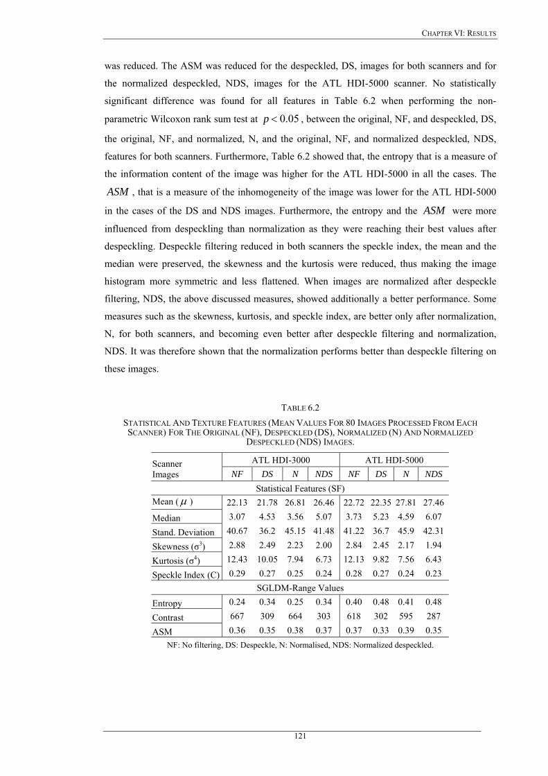
CHAPTER VI: RESULTS
was reduced. The ASM was reduced for the despeckled, DS, images for both scanners and for
the normalized despeckled, NDS, images for the ATL HDI-5000 scanner. No statistically
significant difference was found for all features in Table 6.2 when performing the non-
parametric Wilcoxon rank sum test at 05.0<p , between the original, NF, and despeckled, DS,
the original, NF, and normalized, N, and the original, NF, and normalized despeckled, NDS,
features for both scanners. Furthermore, Table 6.2 showed that, the entropy that is a measure of
the information content of the image was higher for the ATL HDI-5000 in all the cases. The
, that is a measure of the inhomogeneity of the image was lower for the ATL HDI-5000
in the cases of the DS and NDS images. Furthermore, the entropy and the were more
influenced from despeckling than normalization as they were reaching their best values after
despeckling. Despeckle filtering reduced in both scanners the speckle index, the mean and the
median were preserved, the skewness and the kurtosis were reduced, thus making the image
histogram more symmetric and less flattened. When images are normalized after despeckle
filtering, NDS, the above discussed measures, showed additionally a better performance. Some
measures such as the skewness, kurtosis, and speckle index, are better only after normalization,
N, for both scanners, and becoming even better after despeckle filtering and normalization,
NDS. It was therefore shown that the normalization performs better than despeckle filtering on
these images.
ASM
ASM
TABLE 6.2 STATISTICAL AND TEXTURE FEATURES (MEAN VALUES FOR 80 IMAGES PROCESSED FROM EACH SCANNER) FOR THE ORIGINAL (NF), DESPECKLED (DS), NORMALIZED (N) AND NORMALIZED
DESPECKLED (NDS) IMAGES.
ATL HDI-3000 ATL HDI-5000 Scanner Images NF DS N NDS NF DS N NDS
Statistical Features (SF) Mean (µ ) 22.13 21.78 26.81 26.46 22.72 22.35 27.81 27.46
Median 3.07 4.53 3.56 5.07 3.73 5.23 4.59 6.07
Stand. Deviation 40.67 36.2 45.15 41.48 41.22 36.7 45.9 42.31
Skewness (σ3) 2.88 2.49 2.23 2.00 2.84 2.45 2.17 1.94
Kurtosis (σ4) 12.43 10.05 7.94 6.73 12.13 9.82 7.56 6.43
Speckle Index (C) 0.29 0.27 0.25 0.24 0.28 0.27 0.24 0.23 SGLDM-Range Values
Entropy 0.24 0.34 0.25 0.34 0.40 0.48 0.41 0.48
Contrast 667 309 664 303 618 302 595 287
ASM 0.36 0.35 0.38 0.37 0.37 0.33 0.39 0.35 NF: No filtering, DS: Despeckle, N: Normalised, NDS: Normalized despeckled.
121
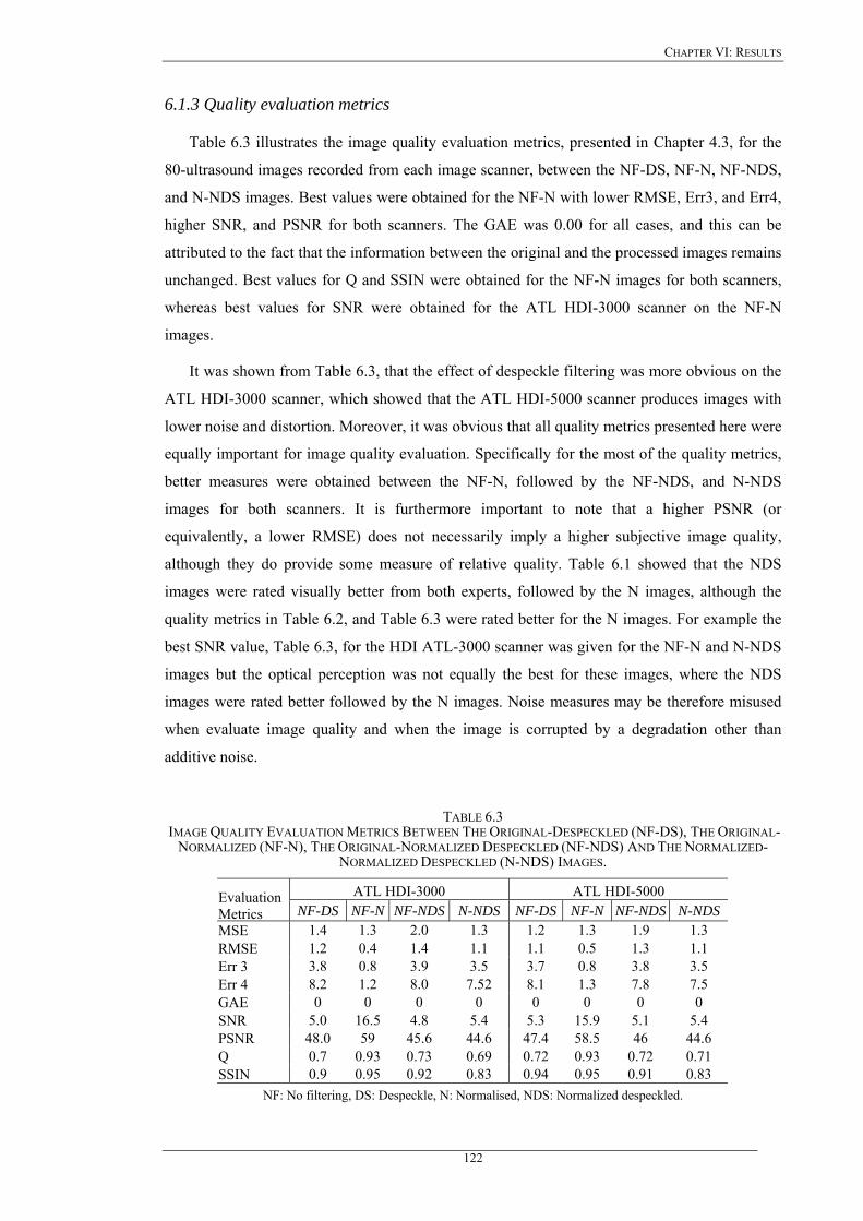
CHAPTER VI: RESULTS
6.1.3 Quality evaluation metrics
Table 6.3 illustrates the image quality evaluation metrics, presented in Chapter 4.3, for the
80-ultrasound images recorded from each image scanner, between the NF-DS, NF-N, NF-NDS,
and N-NDS images. Best values were obtained for the NF-N with lower RMSE, Err3, and Err4,
higher SNR, and PSNR for both scanners. The GAE was 0.00 for all cases, and this can be
attributed to the fact that the information between the original and the processed images remains
unchanged. Best values for Q and SSIN were obtained for the NF-N images for both scanners,
whereas best values for SNR were obtained for the ATL HDI-3000 scanner on the NF-N
images.
It was shown from Table 6.3, that the effect of despeckle filtering was more obvious on the
ATL HDI-3000 scanner, which showed that the ATL HDI-5000 scanner produces images with
lower noise and distortion. Moreover, it was obvious that all quality metrics presented here were
equally important for image quality evaluation. Specifically for the most of the quality metrics,
better measures were obtained between the NF-N, followed by the NF-NDS, and N-NDS
images for both scanners. It is furthermore important to note that a higher PSNR (or
equivalently, a lower RMSE) does not necessarily imply a higher subjective image quality,
although they do provide some measure of relative quality. Table 6.1 showed that the NDS
images were rated visually better from both experts, followed by the N images, although the
quality metrics in Table 6.2, and Table 6.3 were rated better for the N images. For example the
best SNR value, Table 6.3, for the HDI ATL-3000 scanner was given for the NF-N and N-NDS
images but the optical perception was not equally the best for these images, where the NDS
images were rated better followed by the N images. Noise measures may be therefore misused
when evaluate image quality and when the image is corrupted by a degradation other than
additive noise.
TABLE 6.3 IMAGE QUALITY EVALUATION METRICS BETWEEN THE ORIGINAL-DESPECKLED (NF-DS), THE ORIGINAL-
NORMALIZED (NF-N), THE ORIGINAL-NORMALIZED DESPECKLED (NF-NDS) AND THE NORMALIZED-NORMALIZED DESPECKLED (N-NDS) IMAGES.
ATL HDI-3000 ATL HDI-5000 Evaluation Metrics NF-DS NF-N NF-NDS N-NDS NF-DS NF-N NF-NDS N-NDS MSE 1.4 1.3 2.0 1.3 1.2 1.3 1.9 1.3 RMSE 1.2 0.4 1.4 1.1 1.1 0.5 1.3 1.1 Err 3 3.8 0.8 3.9 3.5 3.7 0.8 3.8 3.5 Err 4 8.2 1.2 8.0 7.52 8.1 1.3 7.8 7.5 GAE 0 0 0 0 0 0 0 0 SNR 5.0 16.5 4.8 5.4 5.3 15.9 5.1 5.4 PSNR 48.0 59 45.6 44.6 47.4 58.5 46 44.6 Q 0.7 0.93 0.73 0.69 0.72 0.93 0.72 0.71 SSIN 0.9 0.95 0.92 0.83 0.94 0.95 0.91 0.83
NF: No filtering, DS: Despeckle, N: Normalised, NDS: Normalized despeckled.
122
CHAPTER VI: RESULTS
The two experts evaluated furthermore visually, 10 B-mode ultrasound images with
different types of plaque (type I-type V) [238], as shown in Fig. 5.7. In order to be able to
identify the type of plaque, they have inspected the blood flow image (Fig. 5.7a). The visual
evaluation results showed that the plaques recorded by the ATL HDI-5000 scanner were more
easily identified. The visual perception evaluation of the 10 B-mode ultrasound plaque images,
showed that the plaque may be better identified on the ATL HDI-5000 scanner after
normalization and despeckle filtering, NDS, where the borders of the plaque and the
surrounding tissue may be better visualized, compared with the ATL HDI-3000 scanner.
Specifically when inspecting dangerous plaques, with more that 70% of stenosis, with the ATL
HDI-5000 scanner, the vascular experts were able to identify them better, and thus sparing
patients from an unnecessary operation. The experts stated that, the risk of stroke might be
better identified when using the ATL HDI-5000 scanner, or when using despeckling on the ATL
HDI-3000 scanner. Furthermore, type I, and type V, plaques, which are usually excluded from
different studies, were rated visually better on the ATL HDI-5000 scanner.
123
CHAPTER VI: RESULTS
6.2 Despeckle filtering
In this Section we present the results of the despeckle filters described in Chapter 2, and
evaluate their performance on 220 asymptomatic and 220 symptomatic longitudinal ultrasound
images of the carotid artery. A total of 56 texture features, as presented in Chapter 4.4, were
computed from each image before and after despeckle filtering, from which only the most
discriminant ones, are presented. Furthermore, following the methodology presented in Chapter
5.6, the performance of these filters was investigated using the visual perception evaluation
performed by two vascular experts (section 5.6.1), texture analysis, the Wilcoxon rank sum test,
the statistical kNN classifier (section 5.6.2), and nine different image quality evaluation metrics
(section 5.6.3).
6.2.1 Despeckle filtering on an artificial and a real carotid image
Despeckle filtering was evaluated on an artificial carotid artery image (see Fig. 6.3a),
corrupted by speckle noise as described in section 5.4.
Figure 6.3 shows the original noisy image of the artificial carotid artery, degraded by speckle
noise, together with the despeckled images. Figure 6.4 shows line profiles (intensity), for the
line marked in Fig. 6.3a for all despeckle filters. The profile results show that most of the filters
(median, wiener, lsmv, waveltc, lsminsc, and gf4d), preserved the edge boundaries preserving
the locality and minimally affecting the reference values in each region (as documented in
Chapter 5.6). Best results were given for the filters median, wiener, lsmv, lsminsc, and gf4d. The
filters ad, nldif, ls, waveltc, homog, and homo do not preserve the edges, moving the line
profiles to darker grayscale values. Moreover, it is shown from Fig. 6.4i, that the filter homo is
very noisy.
124

CHAPTER VI: RESULTS
(a) original noisy image. (b) lsmv. (c) lsminsc.
(d) median. (e) wiener. (f) ls.
(g) homog. (h) gf4d. (i) homo.
(j) ad. (k) nldif. (l) waveltc.
Fig. 6.3: Original noisy image of an artificial carotid artery given in (a), and the application of the 11 despeckle filters given in (b)-(l). (Vertical line given in (a) defines the position of the line intensity profiles plotted in Fig. 6.4).
125
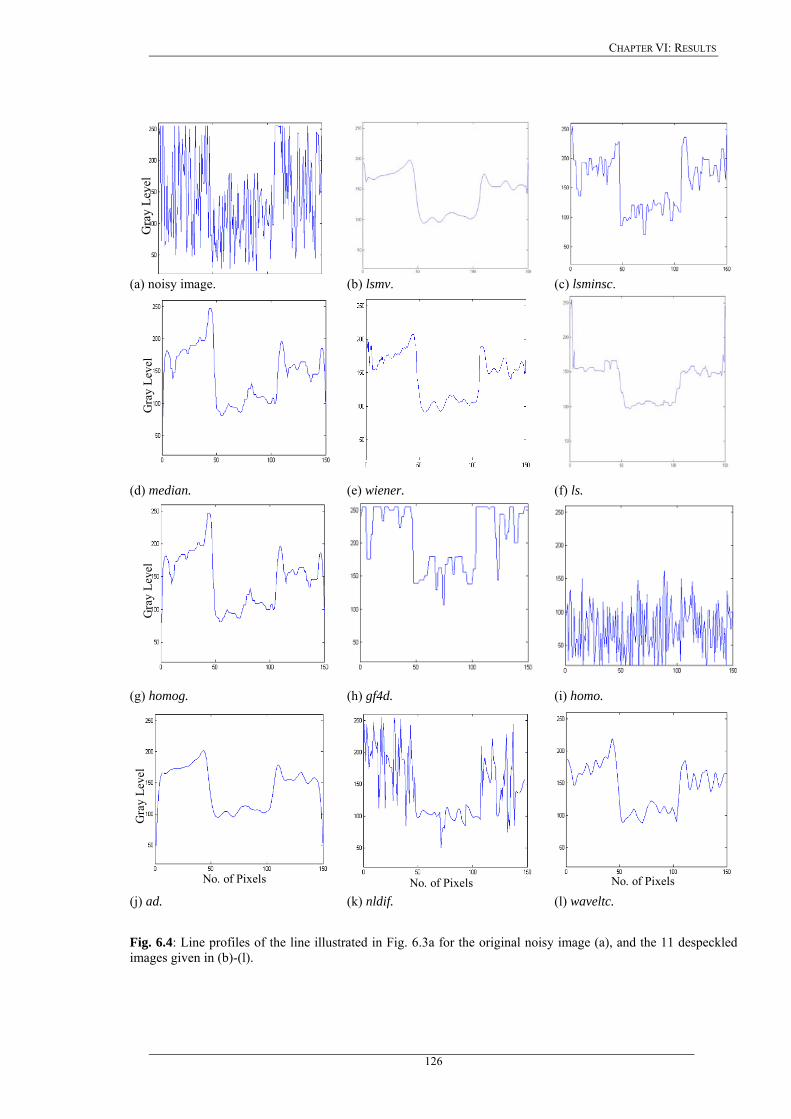
CHAPTER VI: RESULTS
G
ray
Leve
l
(a) noisy image. (b) lsmv. (c) lsminsc.
Gra
y Le
vel
(d) median. (e) wiener. (f) ls.
Gra
y Le
vel
(g) homog. (h) gf4d. (i) homo.
No. of Pixels
Gra
y Le
vel
No. of Pixels
No. of Pixels (j) ad. (k) nldif. (l) waveltc.
Fig. 6.4: Line profiles of the line illustrated in Fig. 6.3a for the original noisy image (a), and the 11 despeckled images given in (b)-(l).
126
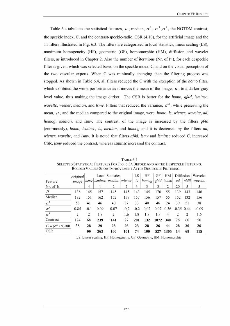
CHAPTER VI: RESULTS
Table 6.4 tabulates the statistical features, µ , median, , , , the NGTDM contrast,
the speckle index, C, and the contrast-speckle-radio, CSR (4.10), for the artificial image and the
11 filters illustrated in Fig. 6.3. The filters are categorized in local statistics, linear scaling (LS),
maximum homogeneity (HF), geometric (GF), homomorphic (HM), diffusion and wavelet
filters, as introduced in Chapter 2. Also the number of iterations (Nr. of It.), for each despeckle
filter is given, which was selected based on the speckle index, C, and on the visual perception of
the two vascular experts. When C was minimally changing then the filtering process was
stopped. As shown in Table 6.4, all filters reduced the C with the exception of the homo filter,
which exhibited the worst performance as it moves the mean of the image,
2σ 3σ 4σ
µ , to a darker gray
level value, thus making the image darker. The CSR is better for the homo, gf4d, lsminsc,
waveltc, wiener, median, and lsmv. Filters that reduced the variance, , while preserving the
mean,
2σ
µ , and the median compared to the original image, were: homo, ls, wiener, waveltc, ad,
homog, median, and lsmv. The contrast, of the image is increased by the filters gf4d
(enormously), homo, lsminsc, ls, median, and homog and it is decreased by the filters ad,
wiener, waveltc, and lsmv. It is noted that filters gf4d, lsmv and lsminsc reduced C, increased
CSR, lsmv reduced the contrast, whereas lsminsc increased the contrast.
TABLE 6.4 SELECTED STATISTICAL FEATURES FOR FIG. 6.3A BEFORE AND AFTER DESPECKLE FILTERING.
BOLDED VALUES SHOW IMPROVEMENT AFTER DESPECKLE FILTERING.
Local Statistics LS HF GF HM Diffusion WaveletFeature
original image lsmv lsminsc median wiener ls homog gf4d homo ad nldif waveltc
Nr. of It. 4 1 2 2 3 3 3 2 20 5 5 µ 138 145 157 145 145 143 145 176 55 139 143 146 Median 132 151 162 152 157 157 156 157 55 152 132 156
2σ 53 41 46 40 37 33 40 46 24 39 51 38 3σ 0.85 -0.1 0.09 0.07 -0.2 -0.2 0.02 0.07 0.36 -0.35 0.44 -0.09 4σ 2 2 1.8 2 1.6 1.8 1.8 1.8 4 2 2 1.6
Contrast 124 68 239 141 27 201 132 1072 340 26 60 50 100)/( 2 µσ=C 38 28 29 28 26 23 28 26 44 28 36 26
CSR 99 263 100 101 74 100 527 1305 14 68 115 LS: Linear scaling, HF: Homogeneity, GF: Geometric, HM: Homomorphic.
127
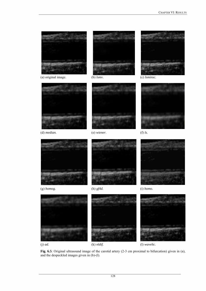
CHAPTER VI: RESULTS
(a) original image. (b) lsmv. (c) lsminsc.
(d) median. (e) wiener. (f) ls.
(g) homog. (h) gf4d. (i) homo.
(j) ad. (k) nldif. (l) waveltc.
Fig. 6.5: Original ultrasound image of the carotid artery (2-3 cm proximal to bifurcation) given in (a), and the despeckled images given in (b)-(l).
128
CHAPTER VI: RESULTS
The despeckled images of Fig. 6.3 were also assessed by the two experts. Filters that showed an
improved smoothing after filtering, as assessed visually by the two experts, using visual
perception criteria, are presented in the following order: waveltc, lsmv, nldif, ad, gf4d and
median. Filters that showed a blurring effect especially on the edges were: ls, lsminsc, homog,
homo and wiener.
Figure 6.5 shows an original longitudinal ultrasound image of a symptomatic carotid artery
together with the despeckled images. The best visual results as assessed by the two vascular
experts were obtained by the filters lsminsc, and lsmv whereas the filters gf4d, ad, and nldif also
show good visual results but, smooth the image considerably and thus edges and subtle details
may be lost. Filters that showed a blurring effect are median, wiener, ls, homog, and waveltc.
Filters wiener, homog, and waveltc showed poorer visual results.
6.2.2 Texture analysis
Despeckle filtering, and texture analysis, were carried out on 440 carotid plaque ultrasound
images (220 asymptomatic, 220 symptomatic). Table 6.5 tabulates the results of feature
distance, , (4.13), and score distance, , (4.14), for SF, SGLDM range of
values and NGTDM feature sets. The results of these feature sets are presented only, since
these sets were the ones with the best performance. The values in bold represent the values that
showed an improvement after despeckle filtering when compared to the original. The last row in
each sub-table shows the for all features, as given in (4.14), where the highest
value indicates the best filter in the sub-table. Additionally a total score distance
was calculated for all feature sets and it is shown in the last row of Table 6.5.
Some of the despeckle filters, shown in Table 6.5, are changing a number of texture features, by
increasing the distance between the two classes, (asymptomatic and symptomatic), and therefore
making the identification and separation of asymptomatic, and symptomatic plaques more
feasible. The positive values in Table 6.5 shows an increase between the two classes whereas
the negative a deterioration.
idisfeat _ DisScore _
DisScore _
TDisScore __
In the first part of the Table 6.5 the results of the statistical features, SF, are presented,
where the best was given by the homo filter followed by the lsminsc, lsmv, homog,
nldif, waveltc, ls, median, and wiener, with the worst given by gf4d. All filters
reduced the speckle index, C. Almost all filters reduced the kurtosis, , and the asymmetry,
, of the histogram, as it may be seen from the bolded values in the first part of Table 6.5.
DisScore _
DisScore _3σ
4σ
In the second part of the Table 6.5 the results of the SGLDM range of values features set are
tabulated. The filters with the highest in the SGLDM range of values features set,
are homo, lsminsc, median, and ad whereas the filters nldif and gf4d are presenting a low
DisScore _
129
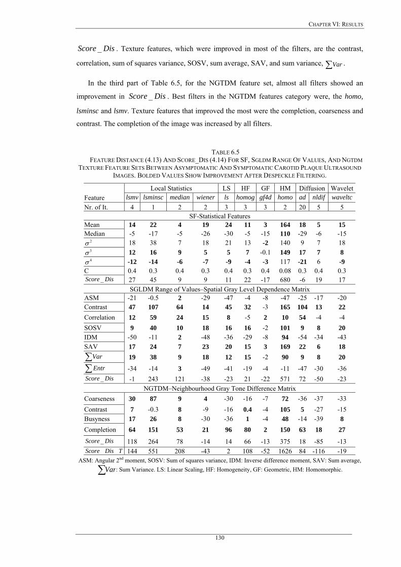
CHAPTER VI: RESULTS
DisScore _ . Texture features, which were improved in most of the filters, are the contrast,
correlation, sum of squares variance, SOSV, sum average, SAV, and sum variance, . ∑Var
In the third part of Table 6.5, for the NGTDM feature set, almost all filters showed an
improvement in . Best filters in the NGTDM features category were, the homo,
lsminsc and lsmv. Texture features that improved the most were the completion, coarseness and
contrast. The completion of the image was increased by all filters.
DisScore _
TABLE 6.5 FEATURE DISTANCE (4.13) AND SCORE_DIS (4.14) FOR SF, SGLDM RANGE OF VALUES, AND NGTDM
TEXTURE FEATURE SETS BETWEEN ASYMPTOMATIC AND SYMPTOMATIC CAROTID PLAQUE ULTRASOUND IMAGES. BOLDED VALUES SHOW IMPROVEMENT AFTER DESPECKLE FILTERING.
Local Statistics LS HF GF HM Diffusion WaveletFeature lsmv lsminsc median wiener ls homog gf4d homo ad nldif waveltcNr. of It. 4 1 2 2 3 3 3 2 20 5 5
SF-Statistical Features Mean 14 22 4 19 24 11 3 164 18 5 15 Median -5 -17 -5 -26 -30 -5 -15 110 -29 -6 -15
2σ 18 38 7 18 21 13 -2 140 9 7 18 3σ 12 16 9 5 5 7 -0.1 149 17 7 8 4σ -12 -14 -6 -7 -9 -4 -3 117 -21 6 -9
C 0.4 0.3 0.4 0.3 0.4 0.3 0.4 0.08 0.3 0.4 0.3 DisScore _ 27 45 9 9 11 22 -17 680 -6 19 17
SGLDM Range of Values–Spatial Gray Level Dependence Matrix ASM -21 -0.5 2 -29 -47 -4 -8 -47 -25 -17 -20 Contrast 47 107 64 14 45 32 -3 165 104 13 22 Correlation 12 59 24 15 8 -5 2 10 54 -4 -4 SOSV 9 40 10 18 16 16 -2 101 9 8 20 IDM -50 -11 2 -48 -36 -29 -8 94 -54 -34 -43 SAV 17 24 7 23 20 15 3 169 22 6 18
∑Var 19 38 9 18 12 15 -2 90 9 8 20
∑Entr -34 -14 3 -49 -41 -19 -4 -11 -47 -30 -36 DisScore _ -1 243 121 -38 -23 21 -22 571 72 -50 -23
NGTDM–Neighbourhood Gray Tone Difference Matrix Coarseness 30 87 9 4 -30 -16 -7 72 -36 -37 -33 Contrast 7 -0.3 8 -9 -16 0.4 -4 105 5 -27 -15 Busyness 17 26 8 -30 -36 1 -4 48 -14 -39 8 Completion 64 151 53 21 96 80 2 150 63 18 27
DisScore _ 118 264 78 -14 14 66 -13 375 18 -85 -13 TDisScore __ 144 551 208 -43 2 108 -52 1626 84 -116 -19
ASM: Angular 2nd moment, SOSV: Sum of squares variance, IDM: Inverse difference moment, SAV: Sum average,
∑Var: Sum Variance. LS: Linear Scaling, HF: Homogeneity, GF: Geometric, HM: Homomorphic.
130
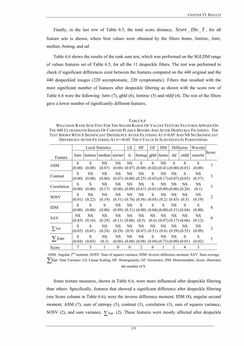
CHAPTER VI: RESULTS
Finally, in the last row of Table 6.5, the total score distance, , for all
feature sets is shown, where best values were obtained by the filters homo, lsminsc, lsmv,
median, homog, and ad.
TDisScore __
Table 6.6 shows the results of the rank sum test, which was performed on the SGLDM range
of values features set of Table 6.5, for all the 11 despeckle filters. The test was performed to
check if significant differences exist between the features computed on the 440 original and the
440 despeckled images (220 asymptomatic, 220 symptomatic). Filters that resulted with the
most significant number of features after despeckle filtering as shown with the score row of
Table 6.6 were the following: lsmv (7), gf4d (6), lsminsc (5) and nldif (4). The rest of the filters
gave a lower number of significantly different features.
TABLE 6.6 WILCOXON RANK SUM TEST FOR THE SGLDM RANGE OF VALUES TEXTURE FEATURES APPLIED ON
THE 440 ULTRASOUND IMAGES OF CAROTID PLAQUE BEFORE AND AFTER DESPECKLE FILTERING. THE TEST SHOWS WITH S SIGNIFICANT DIFFERENCE AFTER FILTERING AT P<0.05 AND NS NO SIGNIFICANT
DIFFERENCE AFTER FILTERING AT P>=0.05. THE P VALUE IS ALSO GIVEN IN PARENTHESIS.
Local Statistics LS HF GF HM Diffusion Wavelet
Feature lsmv lsminsc median wiener ls homog gf4d homo Ad nldif waveltcScore
ASM S (0.00)
S (0.00)
NS (0.07)
NS (0.06)
NS (0.07)
S (0.00)
S (0.02)
NS (0.41)
S (0.00)
S (0.01)
S (0.00) 7
Contrast S (0.00)
NS (0.08)
NS (0.06)
NS (0.07)
NS (0.08)
NS (0.25)
S (0.03)
NS (0.17)
NS (0.07)
S (0.03)
NS (0.57) 3
Correlation S (0.00)
S (0.00)
NS (0.17)
NS (0.06)
NS (0.09)
NS (0.67)
S (0.01)
NS (0.09)
NS (0.06)
NS (0.26)
NS (0.1) 3
SOSV S (0.01)
NS (0.22)
NS (0.19)
NS (0.31)
NS (0.76)
NS (0.56)
S (0.05)
NS (0.2)
NS (0.43)
NS (0.5)
NS (0.19) 2
IDM S (0.00)
S (0.00)
S (0.00)
NS (0.09)
NS (0.31)
S (0.00)
S (0.04)
S (0.00)
NS (0.51)
S (0.04)
S (0.00) 8
SAV NS (0.85)
NS (0.16)
NS (0.29)
NS (0.11)
NS (0.06)
NS (0.5)
NS (0.6)
NS (0.07)
NS (0.17)
NS (0.66)
NS (0.12) 0
∑ Var S (0.02)
S (0.01)
NS (0.24)
NS (0.29)
NS (0.9)
NS (0.47)
NS (0.51)
NS (0.6)
NS (0.59)
NS (0.55)
NS (0.09) 2
∑ Entr S (0.04)
S (0.03)
NS (0.3)
NS (0.06)
NS (0.08)
NS (0.08)
S (0.04)
NS (0.73)
NS (0.09)
S (0.01)
S (0.02) 5
Score 7 5 1 0 0 2 6 1 1 4 3
ASM: Angular 2nd moment, SOSV: Sum of squares variance, IDM: Inverse difference moment, SAV: Sum average,
∑Var: Sum Variance. LS: Linear Scaling, HF: Homogeneity, GF: Geometric, HM: Homomorphic, Score: illustrates
the number of S.
Some texture measures, shown in Table 6.6, were more influenced after despeckle filtering
than others. Specifically, features that showed a significant difference after despeckle filtering
(see Score column in Table 6.6), were the inverse difference moment, IDM (8), angular second
moment, ASM (7), sum of entropy (5), contrast (3), correlation (3), sum of squares variance,
SOSV (2), and sum variance, ∑Var (2). These features were mostly affected after despeckle
131
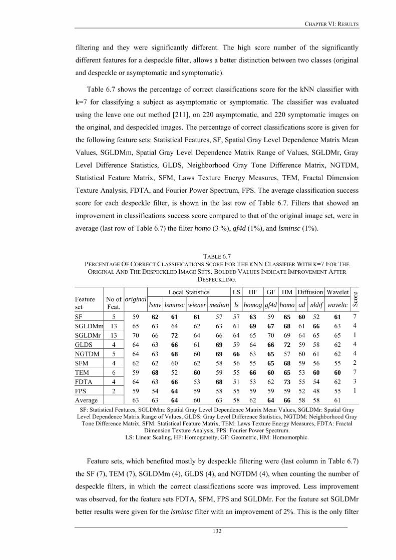
CHAPTER VI: RESULTS
filtering and they were significantly different. The high score number of the significantly
different features for a despeckle filter, allows a better distinction between two classes (original
and despeckle or asymptomatic and symptomatic).
Table 6.7 shows the percentage of correct classifications score for the kNN classifier with
k=7 for classifying a subject as asymptomatic or symptomatic. The classifier was evaluated
using the leave one out method [211], on 220 asymptomatic, and 220 symptomatic images on
the original, and despeckled images. The percentage of correct classifications score is given for
the following feature sets: Statistical Features, SF, Spatial Gray Level Dependence Matrix Mean
Values, SGLDMm, Spatial Gray Level Dependence Matrix Range of Values, SGLDMr, Gray
Level Difference Statistics, GLDS, Neighborhood Gray Tone Difference Matrix, NGTDM,
Statistical Feature Matrix, SFM, Laws Texture Energy Measures, TEM, Fractal Dimension
Texture Analysis, FDTA, and Fourier Power Spectrum, FPS. The average classification success
score for each despeckle filter, is shown in the last row of Table 6.7. Filters that showed an
improvement in classifications success score compared to that of the original image set, were in
average (last row of Table 6.7) the filter homo (3 %), gf4d (1%), and lsminsc (1%).
TABLE 6.7 PERCENTAGE OF CORRECT CLASSIFICATIONS SCORE FOR THE KNN CLASSIFIER WITH K=7 FOR THE ORIGINAL AND THE DESPECKLED IMAGE SETS. BOLDED VALUES INDICATE IMPROVEMENT AFTER
DESPECKLING.
Local Statistics LS HF GF HM Diffusion WaveletFeature set
No of Feat.
original lsmv lsminsc wiener median ls homog gf4d homo ad nldif waveltc Sc
ore
SF 5 59 62 61 61 57 57 63 59 65 60 52 61 7SGLDMm 13 65 63 64 62 63 61 69 67 68 61 66 63 4SGLDMr 13 70 66 72 64 66 64 65 70 69 64 65 65 1GLDS 4 64 63 66 61 69 59 64 66 72 59 58 62 4NGTDM 5 64 63 68 60 69 66 63 65 57 60 61 62 4SFM 4 62 62 60 62 58 56 55 65 68 59 56 55 2TEM 6 59 68 52 60 59 55 66 60 65 53 60 60 7FDTA 4 64 63 66 53 68 51 53 62 73 55 54 62 3FPS 2 59 54 64 59 58 55 59 59 59 52 48 55 1Average 63 63 64 60 63 58 62 64 66 58 58 61
SF: Statistical Features, SGLDMm: Spatial Gray Level Dependence Matrix Mean Values, SGLDMr: Spatial Gray Level Dependence Matrix Range of Values, GLDS: Gray Level Difference Statistics, NGTDM: Neighborhood Gray
Tone Difference Matrix, SFM: Statistical Feature Matrix, TEM: Laws Texture Energy Measures, FDTA: Fractal Dimension Texture Analysis, FPS: Fourier Power Spectrum.
LS: Linear Scaling, HF: Homogeneity, GF: Geometric, HM: Homomorphic.
Feature sets, which benefited mostly by despeckle filtering were (last column in Table 6.7)
the SF (7), TEM (7), SGLDMm (4), GLDS (4), and NGTDM (4), when counting the number of
despeckle filters, in which the correct classifications score was improved. Less improvement
was observed, for the feature sets FDTA, SFM, FPS and SGLDMr. For the feature set SGLDMr
better results were given for the lsminsc filter with an improvement of 2%. This is the only filter
132
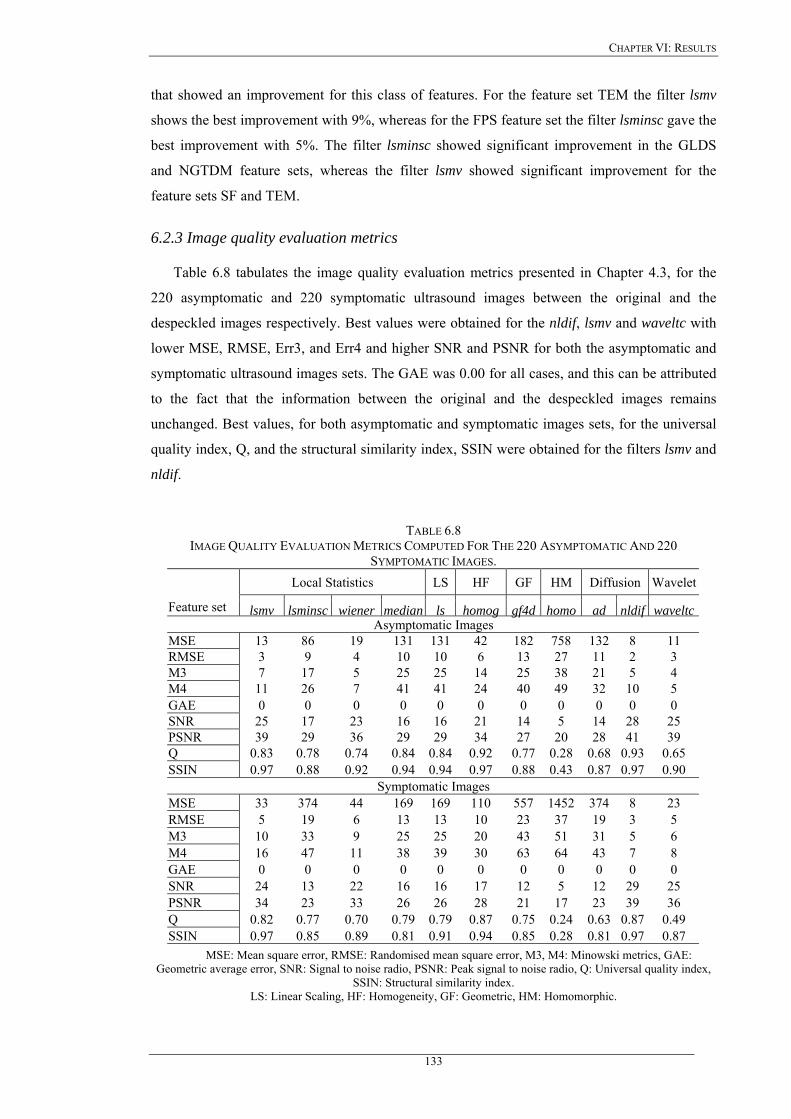
CHAPTER VI: RESULTS
that showed an improvement for this class of features. For the feature set TEM the filter lsmv
shows the best improvement with 9%, whereas for the FPS feature set the filter lsminsc gave the
best improvement with 5%. The filter lsminsc showed significant improvement in the GLDS
and NGTDM feature sets, whereas the filter lsmv showed significant improvement for the
feature sets SF and TEM.
6.2.3 Image quality evaluation metrics
Table 6.8 tabulates the image quality evaluation metrics presented in Chapter 4.3, for the
220 asymptomatic and 220 symptomatic ultrasound images between the original and the
despeckled images respectively. Best values were obtained for the nldif, lsmv and waveltc with
lower MSE, RMSE, Err3, and Err4 and higher SNR and PSNR for both the asymptomatic and
symptomatic ultrasound images sets. The GAE was 0.00 for all cases, and this can be attributed
to the fact that the information between the original and the despeckled images remains
unchanged. Best values, for both asymptomatic and symptomatic images sets, for the universal
quality index, Q, and the structural similarity index, SSIN were obtained for the filters lsmv and
nldif.
TABLE 6.8 IMAGE QUALITY EVALUATION METRICS COMPUTED FOR THE 220 ASYMPTOMATIC AND 220
SYMPTOMATIC IMAGES. Local Statistics LS HF GF HM Diffusion Wavelet
Feature set lsmv lsminsc wiener median ls homog gf4d homo ad nldif waveltcAsymptomatic Images
MSE 13 86 19 131 131 42 182 758 132 8 11 RMSE 3 9 4 10 10 6 13 27 11 2 3 M3 7 17 5 25 25 14 25 38 21 5 4 M4 11 26 7 41 41 24 40 49 32 10 5 GAE 0 0 0 0 0 0 0 0 0 0 0 SNR 25 17 23 16 16 21 14 5 14 28 25 PSNR 39 29 36 29 29 34 27 20 28 41 39 Q 0.83 0.78 0.74 0.84 0.84 0.92 0.77 0.28 0.68 0.93 0.65 SSIN 0.97 0.88 0.92 0.94 0.94 0.97 0.88 0.43 0.87 0.97 0.90
Symptomatic Images MSE 33 374 44 169 169 110 557 1452 374 8 23 RMSE 5 19 6 13 13 10 23 37 19 3 5 M3 10 33 9 25 25 20 43 51 31 5 6 M4 16 47 11 38 39 30 63 64 43 7 8 GAE 0 0 0 0 0 0 0 0 0 0 0 SNR 24 13 22 16 16 17 12 5 12 29 25 PSNR 34 23 33 26 26 28 21 17 23 39 36 Q 0.82 0.77 0.70 0.79 0.79 0.87 0.75 0.24 0.63 0.87 0.49 SSIN 0.97 0.85 0.89 0.81 0.91 0.94 0.85 0.28 0.81 0.97 0.87
MSE: Mean square error, RMSE: Randomised mean square error, M3, M4: Minowski metrics, GAE: Geometric average error, SNR: Signal to noise radio, PSNR: Peak signal to noise radio, Q: Universal quality index,
SSIN: Structural similarity index. LS: Linear Scaling, HF: Homogeneity, GF: Geometric, HM: Homomorphic.
133
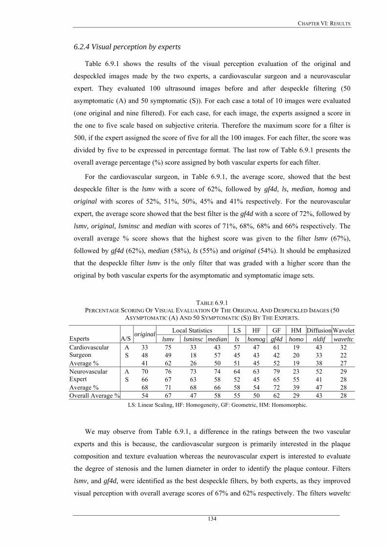
CHAPTER VI: RESULTS
6.2.4 Visual perception by experts
Table 6.9.1 shows the results of the visual perception evaluation of the original and
despeckled images made by the two experts, a cardiovascular surgeon and a neurovascular
expert. They evaluated 100 ultrasound images before and after despeckle filtering (50
asymptomatic (A) and 50 symptomatic (S)). For each case a total of 10 images were evaluated
(one original and nine filtered). For each case, for each image, the experts assigned a score in
the one to five scale based on subjective criteria. Therefore the maximum score for a filter is
500, if the expert assigned the score of five for all the 100 images. For each filter, the score was
divided by five to be expressed in percentage format. The last row of Table 6.9.1 presents the
overall average percentage (%) score assigned by both vascular experts for each filter.
For the cardiovascular surgeon, in Table 6.9.1, the average score, showed that the best
despeckle filter is the lsmv with a score of 62%, followed by gf4d, ls, median, homog and
original with scores of 52%, 51%, 50%, 45% and 41% respectively. For the neurovascular
expert, the average score showed that the best filter is the gf4d with a score of 72%, followed by
lsmv, original, lsminsc and median with scores of 71%, 68%, 68% and 66% respectively. The
overall average % score shows that the highest score was given to the filter lsmv (67%),
followed by gf4d (62%), median (58%), ls (55%) and original (54%). It should be emphasized
that the despeckle filter lsmv is the only filter that was graded with a higher score than the
original by both vascular experts for the asymptomatic and symptomatic image sets.
TABLE 6.9.1 PERCENTAGE SCORING OF VISUAL EVALUATION OF THE ORIGINAL AND DESPECKLED IMAGES (50
ASYMPTOMATIC (A) AND 50 SYMPTOMATIC (S)) BY THE EXPERTS.
Local Statistics LS HF GF HM Diffusion WaveletExperts A/S
original lsmv lsminsc median ls homog gf4d homo nldif waveltc
A 33 75 33 43 57 47 61 19 43 32 Cardiovascular Surgeon S 48 49 18 57 45 43 42 20 33 22 Average % 41 62 26 50 51 45 52 19 38 27
A 70 76 73 74 64 63 79 23 52 29 Neurovascular Expert S 66 67 63 58 52 45 65 55 41 28 Average % 68 71 68 66 58 54 72 39 47 28 Overall Average % 54 67 47 58 55 50 62 29 43 28
LS: Linear Scaling, HF: Homogeneity, GF: Geometric, HM: Homomorphic.
We may observe from Table 6.9.1, a difference in the ratings between the two vascular
experts and this is because, the cardiovascular surgeon is primarily interested in the plaque
composition and texture evaluation whereas the neurovascular expert is interested to evaluate
the degree of stenosis and the lumen diameter in order to identify the plaque contour. Filters
lsmv, and gf4d, were identified as the best despeckle filters, by both experts, as they improved
visual perception with overall average scores of 67% and 62% respectively. The filters waveltc
134
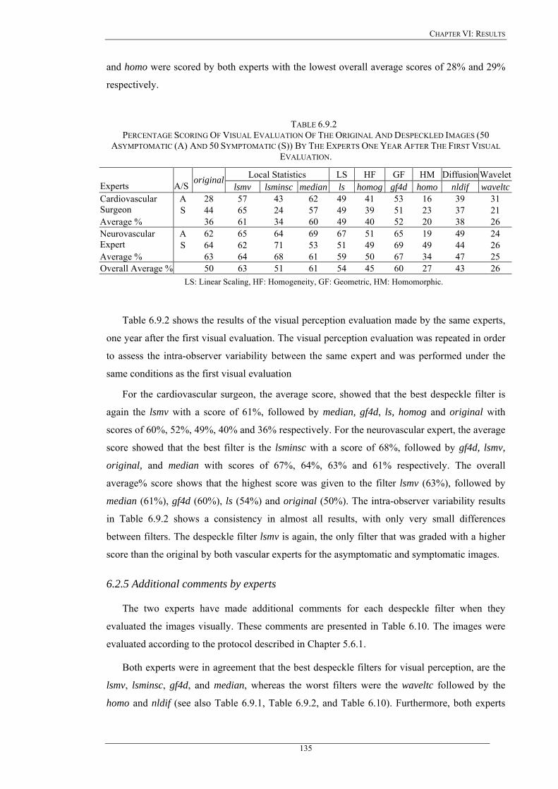
CHAPTER VI: RESULTS
and homo were scored by both experts with the lowest overall average scores of 28% and 29%
respectively.
TABLE 6.9.2 PERCENTAGE SCORING OF VISUAL EVALUATION OF THE ORIGINAL AND DESPECKLED IMAGES (50
ASYMPTOMATIC (A) AND 50 SYMPTOMATIC (S)) BY THE EXPERTS ONE YEAR AFTER THE FIRST VISUAL EVALUATION.
Local Statistics LS HF GF HM Diffusion WaveletExperts A/S original
lsmv lsminsc median ls homog gf4d homo nldif waveltcA 28 57 43 62 49 41 53 16 39 31 Cardiovascular
Surgeon S 44 65 24 57 49 39 51 23 37 21 Average % 36 61 34 60 49 40 52 20 38 26
A 62 65 64 69 67 51 65 19 49 24 Neurovascular Expert S 64 62 71 53 51 49 69 49 44 26 Average % 63 64 68 61 59 50 67 34 47 25 Overall Average % 50 63 51 61 54 45 60 27 43 26
LS: Linear Scaling, HF: Homogeneity, GF: Geometric, HM: Homomorphic.
Table 6.9.2 shows the results of the visual perception evaluation made by the same experts,
one year after the first visual evaluation. The visual perception evaluation was repeated in order
to assess the intra-observer variability between the same expert and was performed under the
same conditions as the first visual evaluation
For the cardiovascular surgeon, the average score, showed that the best despeckle filter is
again the lsmv with a score of 61%, followed by median, gf4d, ls, homog and original with
scores of 60%, 52%, 49%, 40% and 36% respectively. For the neurovascular expert, the average
score showed that the best filter is the lsminsc with a score of 68%, followed by gf4d, lsmv,
original, and median with scores of 67%, 64%, 63% and 61% respectively. The overall
average% score shows that the highest score was given to the filter lsmv (63%), followed by
median (61%), gf4d (60%), ls (54%) and original (50%). The intra-observer variability results
in Table 6.9.2 shows a consistency in almost all results, with only very small differences
between filters. The despeckle filter lsmv is again, the only filter that was graded with a higher
score than the original by both vascular experts for the asymptomatic and symptomatic images.
6.2.5 Additional comments by experts
The two experts have made additional comments for each despeckle filter when they
evaluated the images visually. These comments are presented in Table 6.10. The images were
evaluated according to the protocol described in Chapter 5.6.1.
Both experts were in agreement that the best despeckle filters for visual perception, are the
lsmv, lsminsc, gf4d, and median, whereas the worst filters were the waveltc followed by the
homo and nldif (see also Table 6.9.1, Table 6.9.2, and Table 6.10). Furthermore, both experts
135
CHAPTER VI: RESULTS
agreed that almost all despeckle filters reduced the noise substantially and images may be better
visualized after despeckle filtering.
By examining all the visual results of Fig. 6.3-Fig. 6.5, the statistical results of Table 6.4-Table
6.8, the visual evaluation of Tables 6.9.1 and Table 6.9.2, and the additional comments made by
the experts in Table 6.10, we can conclude that the best filters are the lsmv and the gf4d, which
may be used for both plaque composition enhancement and plaque texture analysis, whereas the
filters lsmv, gf4d and lsminsc are more suitable to identify the degree of stenosis and therefore
may be used when the primary interest is to outline the plaque borders.
136

CHAPTER VI: RESULTS
TABLE 6.10 ADDITIONAL COMMENTS ON DESPECKLE FILTERING MADE BY THE EXPERTS.
Filter name Comments made by the vascular experts on ultrasound images of the carotid artery
original The plaque, and or IMT borders may not be easily visualized between posterior and
anterior tissue. Therefore the adventitia, at the far wall may not be easily located.
lsmv
It helps to visualize the borders between blood and wall but not very good to visualize the
borders between the wall and the surrounding tissue. It does not blur edges, and it helps
visualizing the plaque borders.
lsminsc
Not very suitable for the far wall and IMT segmentation, but it is one of the best filters,
providing information about the plaque, as the borders of the plaque may be better
distinguished after filtering.
median
Not good for the far wall IMT detection. It blurs, gives double edges and smoothes the
image too much. Helps to locate the boundaries of plaque, but lsminsc is better for plaque
visualization.
wiener It is not bad between blood and wall boundaries but the noise still remains on edges after
filtering. It is, therefore not helpful either for IMT or plaque segmentation.
ls
Although not bad for visual perception, it is not suitable for the IMT and plaque
segmentation, as it blurs homogeneous areas and edges. In some images produces double
edges. It is not very helpful for visualizing the IMT, either in near or far wall of the
carotid artery.
homog Breaks the edges between blood and wall causing blurring between wall and surrounding
tissue. It may help sometimes to locate the boundaries of the far wall (adventitia).
gf4d
It sharpens the edges. It helps to locate the boundaries of the far wall (adventitia) and the
plaque may be better visualized. Borders between blood and plaque may be well
separated.
homo Very bad for border detection and visualization, as the image becomes darker after
filtering. It is therefore not recommended.
ad
Although not very good visually, it may be used in some images to visualize the borders
between wall and blood. It is in general not well suited as a pre-processing step prior to
segmentation of the IMT and plaque borders.
nldif Although good visually, the IMT and plaque borders may be not well distinguished. It is
not very helpful to locate either adventitia, nor intima, nor plaque.
waveltc
The visualization after despeckle filtering, is better between blood and vessel and between
vessel and tissue. Also the walls appear continuous but their contrast is very low. It may
be good for boundary detection between vessel and the surrounding tissue at the near wall.
137
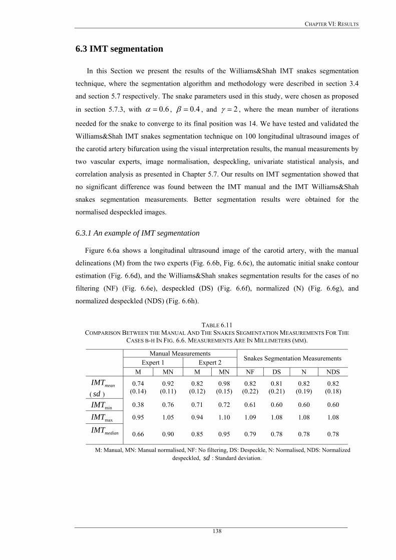
CHAPTER VI: RESULTS
6.3 IMT segmentation
In this Section we present the results of the Williams&Shah IMT snakes segmentation
technique, where the segmentation algorithm and methodology were described in section 3.4
and section 5.7 respectively. The snake parameters used in this study, were chosen as proposed
in section 5.7.3, with 6.0=α , 4.0=β , and 2=γ , where the mean number of iterations
needed for the snake to converge to its final position was 14. We have tested and validated the
Williams&Shah IMT snakes segmentation technique on 100 longitudinal ultrasound images of
the carotid artery bifurcation using the visual interpretation results, the manual measurements by
two vascular experts, image normalisation, despeckling, univariate statistical analysis, and
correlation analysis as presented in Chapter 5.7. Our results on IMT segmentation showed that
no significant difference was found between the IMT manual and the IMT Williams&Shah
snakes segmentation measurements. Better segmentation results were obtained for the
normalised despeckled images.
6.3.1 An example of IMT segmentation
Figure 6.6a shows a longitudinal ultrasound image of the carotid artery, with the manual
delineations (M) from the two experts (Fig. 6.6b, Fig. 6.6c), the automatic initial snake contour
estimation (Fig. 6.6d), and the Williams&Shah snakes segmentation results for the cases of no
filtering (NF) (Fig. 6.6e), despeckled (DS) (Fig. 6.6f), normalized (N) (Fig. 6.6g), and
normalized despeckled (NDS) (Fig. 6.6h).
TABLE 6.11 COMPARISON BETWEEN THE MANUAL AND THE SNAKES SEGMENTATION MEASUREMENTS FOR THE
CASES B-H IN FIG. 6.6. MEASUREMENTS ARE IN MILLIMETERS (MM).
Manual Measurements Expert 1 Expert 2 Snakes Segmentation Measurements
M MN M MN NF DS N NDS
meanIMT ( ) sd
0.74 (0.14)
0.92 (0.11)
0.82 (0.12)
0.98 (0.15)
0.82 (0.22)
0.81 (0.21)
0.82 (0.19)
0.82 (0.18)
minIMT 0.38 0.76 0.71 0.72 0.61 0.60 0.60 0.60
maxIMT 0.95 1.05 0.94 1.10 1.09 1.08 1.08 1.08
medianIMT
0.66 0.90 0.85 0.95 0.79 0.78 0.78 0.78
M: Manual, MN: Manual normalised, NF: No filtering, DS: Despeckle, N: Normalised, NDS: Normalized despeckled, : Standard deviation. sd
138
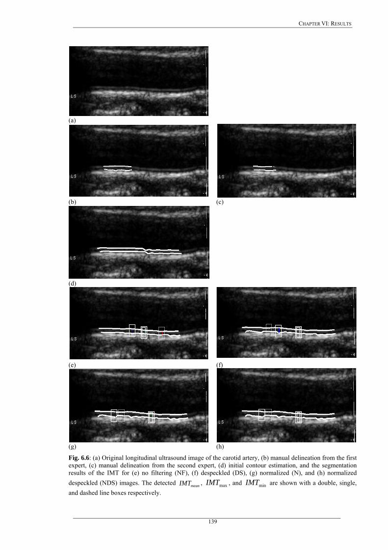
CHAPTER VI: RESULTS
(a)
(b) (c)
(d)
(e) (f)
(g) (h)
Fig. 6.6: (a) Original longitudinal ultrasound image of the carotid artery, (b) manual delineation from the first expert, (c) manual delineation from the second expert, (d) initial contour estimation, and the segmentation results of the IMT for (e) no filtering (NF), (f) despeckled (DS), (g) normalized (N), and (h) normalized despeckled (NDS) images. The detected , , and are shown with a double, single, and dashed line boxes respectively.
meanIMT maxIMT minIMT
139
CHAPTER VI: RESULTS
The detected , , and values, are shown with a double, full, and dashed
line boxes respectively.
meanIMT maxIMT minIMT
The , , , and , measurements for Fig. 6.6 are presented in
Table 6.11. The manual measurements are given for each expert, in cases when manual
measurements were carried out, without normalization (M) and with normalization (MN). The
Williams&Shah snakes segmentation measurements are given for the NF, DS, N and NDS
cases, and were in the most of the cases, higher than the manual measurements, except in the
MN case for both experts. The higher snakes segmentation results can be explained with Fig.
3.1b. The observed standard deviation, , values for the , was for the first expert, M
(0.14), MN (0.11), for the second expert, M (0.12), MN (0.15), and for the snakes segmentation,
NF (0.22), DS (0.21), N (0.19), and NDS (0.18) respectively. The results in Fig. 6.6 and Table
6.11 show, that the IMT was detected well in all snakes segmentation measurements but with
variations between experts and methods. The best visual results as assessed by the two vascular
experts were obtained on the NDS, followed by N and DS images.
meanIMT minIMT maxIMT medianIMT
sd meanIMT
6.3.2 Univariate statistical analysis
Table 6.12.1 tabulates the manual and the Williams&Shah snakes segmentation results for
100 longitudinal ultrasound images of the carotid artery, for the , , and
, with their standard deviations, , inter-observer error,
meanIMT minIMT maxIMT
medianIMT sd se , and coefficient of
variation, . The %CV meanIMT ± standard deviation results for the first expert were,
0.67 0.16 mm, 0.68 0.17 mm, and for the second expert were, 0.65 0.18 mm, 0.61± ± ± ± 0.17
mm on the original and normalized images respectively. The standard deviation
snakes segmentation results were 0.7
meanIMT ±
± 0.14 mm, 0.69± 0.13 mm, 0.67 0.13 mm, 0.68± ± 0.12
mm, for the NF, DS, N, and NDS images respectively. It is noted that both the , and
measurements are very close.
meanIMT
medianIMT
Best segmentation results are shown with bolded values and were obtained for the NDS
images, with a standard deviation of the , meanIMT 12.0=sd mm, an inter-observer error of the
, and a coefficient of variation, meanIMT 08.0=se %5.12% =CV respectively.
Table 6.12.2 presents the manual measurements for 100 images of the carotid artery made by
the two experts one year after the first measurements were made (see Table 6.12.1). This was
carried out by both experts in order to assess the intra-observer variability. It is shown that the
measurements of the second expert, are generally smaller giving a thinner IMT.
140
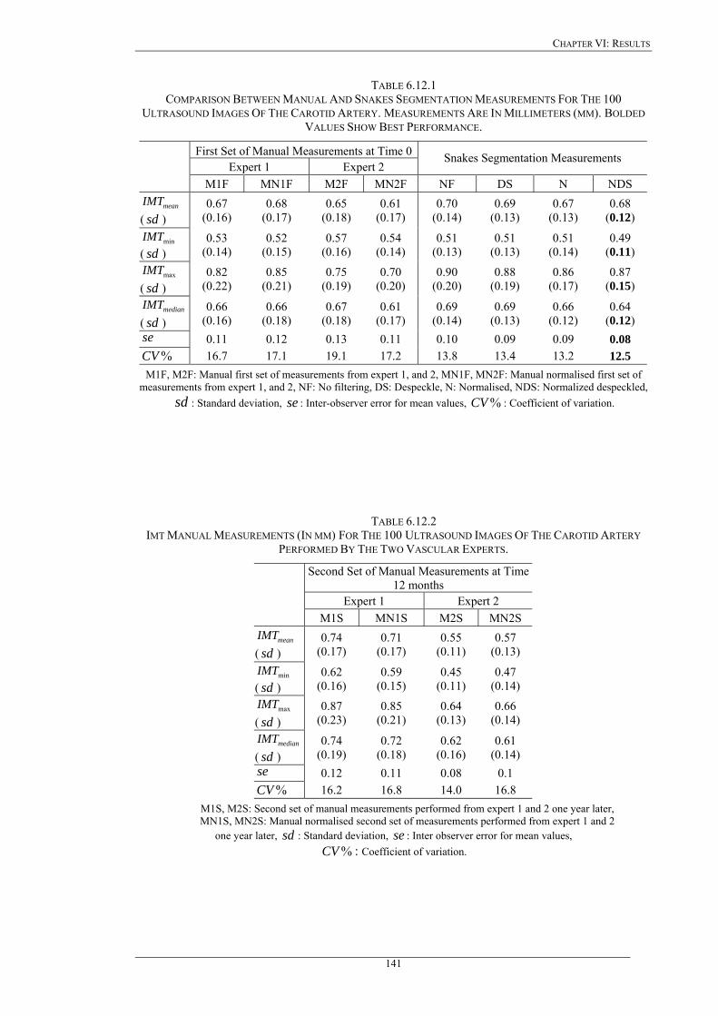
CHAPTER VI: RESULTS
TABLE 6.12.1 COMPARISON BETWEEN MANUAL AND SNAKES SEGMENTATION MEASUREMENTS FOR THE 100
ULTRASOUND IMAGES OF THE CAROTID ARTERY. MEASUREMENTS ARE IN MILLIMETERS (MM). BOLDED VALUES SHOW BEST PERFORMANCE.
First Set of Manual Measurements at Time 0Expert 1 Expert 2
Snakes Segmentation Measurements
M1F MN1F M2F MN2F NF DS N NDS
meanIMT ( ) sd
0.67 (0.16)
0.68 (0.17)
0.65 (0.18)
0.61 (0.17)
0.70 (0.14)
0.69 (0.13)
0.67 (0.13)
0.68 (0.12)
minIMT ( ) sd
0.53 (0.14)
0.52 (0.15)
0.57 (0.16)
0.54 (0.14)
0.51 (0.13)
0.51 (0.13)
0.51 (0.14)
0.49 (0.11)
maxIMT ( ) sd
0.82 (0.22)
0.85 (0.21)
0.75 (0.19)
0.70 (0.20)
0.90 (0.20)
0.88 (0.19)
0.86 (0.17)
0.87 (0.15)
medianIMT ( ) sd
0.66 (0.16)
0.66 (0.18)
0.67 (0.18)
0.61 (0.17)
0.69 (0.14)
0.69 (0.13)
0.66 (0.12)
0.64 (0.12)
se 0.11 0.12 0.13 0.11 0.10 0.09 0.09 0.08 %CV 16.7 17.1 19.1 17.2 13.8 13.4 13.2 12.5
M1F, M2F: Manual first set of measurements from expert 1, and 2, MN1F, MN2F: Manual normalised first set of measurements from expert 1, and 2, NF: No filtering, DS: Despeckle, N: Normalised, NDS: Normalized despeckled,
: Standard deviation, sd se : Inter-observer error for mean values, : Coefficient of variation. %CV
TABLE 6.12.2 IMT MANUAL MEASUREMENTS (IN MM) FOR THE 100 ULTRASOUND IMAGES OF THE CAROTID ARTERY
PERFORMED BY THE TWO VASCULAR EXPERTS.
Second Set of Manual Measurements at Time 12 months
Expert 1 Expert 2
M1S MN1S M2S MN2S
meanIMT ( ) sd
0.74 (0.17)
0.71 (0.17)
0.55 (0.11)
0.57 (0.13)
minIMT ( ) sd
0.62 (0.16)
0.59 (0.15)
0.45 (0.11)
0.47 (0.14)
maxIMT ( ) sd
0.87 (0.23)
0.85 (0.21)
0.64 (0.13)
0.66 (0.14)
medianIMT( ) sd
0.74 (0.19)
0.72 (0.18)
0.62 (0.16)
0.61 (0.14)
se 0.12 0.11 0.08 0.1 %CV 16.2 16.8 14.0 16.8
M1S, M2S: Second set of manual measurements performed from expert 1 and 2 one year later, MN1S, MN2S: Manual normalised second set of measurements performed from expert 1 and 2
one year later, sd : Standard deviation, se : Inter observer error for mean values, %CV : Coefficient of variation.
141
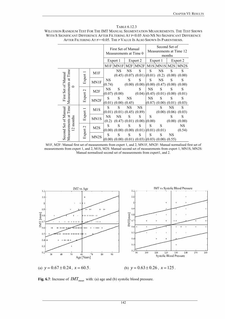
CHAPTER VI: RESULTS
TABLE 6.12.3 WILCOXON RANKSUM TEST FOR THE IMT MANUAL SEGMENTATION MEASUREMENTS. THE TEST SHOWS WITH S SIGNIFICANT DIFFERENCE AFTER FILTERING AT P<0.05 AND NS NO SIGNIFICANT DIFFERENCE
AFTER FILTERING AT P>=0.05. THE P VALUE IS ALSO SHOWN IN PARENTHESIS.
First Set of Manual Measurements at Time 0
Second Set of Measurements at Time 12
months Expert 1 Expert 2 Expert 1 Expert 2
M1F MN1F M2F MN2F M1S MN1S M2S MN2S
M1F NS (0.45)
NS (0.07)
S (0.01)
S (0.01)
NS (0.2)
S (0.00)
S (0.00)
Expe
rt 1
MN1F NS (0.74) S
(0.00)S
(0.00)S
(0.00)NS
(0.47) S
(0.00) S
(0.00)
M2F NS (0.07)
S (0.00) S
(0.04)NS
(0.45)S
(0.01) S
(0.00) S
(0.01)
Firs
t Set
of M
anua
l M
easu
rem
ents
at T
ime
0
Expe
rt 2
MN2F S (0.01)
S (0.00)
NS (0.45) NS
(0.87)S
(0.00) S
(0.01) S
(0.03)
M1S S (0.01)
S (0.01)
NS (0.45)
NS (0.89) S
(0.00) NS
(0.06) S
(0.03)
Expe
rt 1
MN1S NS (0.2)
NS (0.47)
S (0.01)
S (0.00)
S (0.00) S
(0.00) S
(0.00)
M2S S (0.00)
S (0.00)
S (0.00)
S (0.01)
S (0.01)
S (0.01) NS
(0.54)
Seco
nd S
et o
f Man
ual
Mea
sure
men
ts a
t Tim
e 12
mon
ths
Expe
rt 2
MN2S S (0.00)
S (0.00)
S (0.01)
S (0.03)
S (0.03)
S (0.00)
NS (0.55)
M1F, M2F: Manual first set of measurements from expert 1, and 2, MN1F, MN2F: Manual normalised first set of measurements from expert 1, and 2, M1S, M2S: Manual second set of measurements from expert 1, MN1S, MN2S:
Manual normalised second set of measurements from expert1, and 2.
(a) , . 24.067.0 ±=y 5.60=x (b) 26.063.0 ±=y , . 125=x
Fig. 6.7: Increase of with: (a) age and (b) systolic blood pressure. meanIMT
142
CHAPTER VI: RESULTS
Furthermore, the standard deviation, , the inter-observer error, , and the coefficient of
variation, , for the measurements made by the second expert are also smaller.
sd se
%CV
Table 6.12.3 presents the results for the Wilcoxon rank sum test for all manual
segmentation, measurements. It is shown that the measurements made by the two experts are
mostly significantly different (S), showing high intra and inter observer variabilities.
Figure 6.7 presents the results of the values versus age (see Fig. 6.7a), and systolic
blood pressure (see Fig. 6.7b) respectively using regression analysis. It is shown that the
increases almost linearly with increasing age and systolic blood pressure. Furthermore,
it is shown, from Fig. 6.7a, that the , at the age of 60.5 is 0.67 mm, whereas Fig. 6.7b
shows, that the blood pressure for an of 0.63 mm, is 125. Figure 6.7 also shows the
confidence interval limits for the , with
meanIMT
meanIMT
meanIMT
meanIMT
meanIMT ± 0.24 mm, and ± 0.26 mm for age
(seeFig.6.7a), and systolic blood pressure (see Fig. 6.7b) respectively.
Table 6.13.1 shows the results of the Wilcoxon rank sum test, a variation of the Hausdorff
distance (HD), the covariance, and the between the first expert and the snakes
segmentation measurements. The Wilcoxon rank sum test, which is displayed in the upper
triangle of the left column of Table 6.13.1, showed that no-significant (NS) difference exists
between the Williams&Shah snakes segmentation measurements and the manual measurements
from the first expert. The NS difference between the two methods showed that the manual
measurements may be replaced by the snakes segmentation measurements without confidence.
The HD, which is displayed in the left column lower triangle of Table 6.13.1, showed that
minimum mismatches were obtained between the N-M1F (3.4), NDS-MN1F (4.7), NDS-N
(5.2), DS-NF (5.2), NDS-M1F and DS-MN1F (8.6) respectively.
MSE
The covariance is displayed in the upper triangle of the right column of Table 6.13.1.
Higher covariance values were obtained for the cases M1F-MN1F (21.7), NF-DS (16.3), NF-N
(14.4), DS-N (14.4), DS-NDS (13.1), N-NDS (12.9) and NF-NDS (12.8) respectively. MSE
results were shown in the lower triangle of the right column. Low MSE values were observed
for N-M1F (0.01), NDS-MN1F (0.02), NDS-N (0.03) and DS-NF (0.03) respectively.
Table 6.13.2 shows the results of the Wilcoxon rank sum test, a variation of the Hausdorff
distance (HD), the covariance, and the between the second expert and the snakes
segmentation measurements. The Wilcoxon rank sum test, which is displayed in the upper
triangle of the left column of Table 6.13.2, showed that a significant difference (S) between the
manual (M2F) and the manual normalised (MN2F) measurements of the second expert exists.
MSE
143
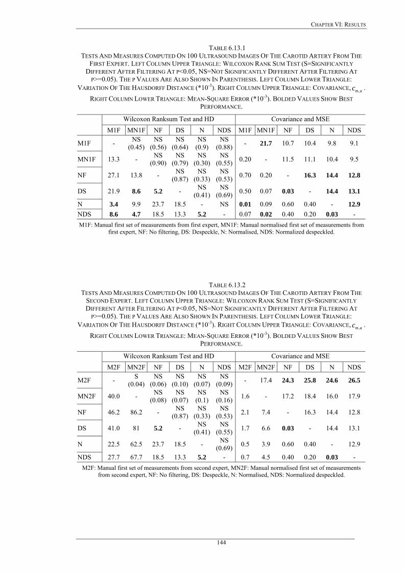
CHAPTER VI: RESULTS
TABLE 6.13.1 TESTS AND MEASURES COMPUTED ON 100 ULTRASOUND IMAGES OF THE CAROTID ARTERY FROM THE
FIRST EXPERT. LEFT COLUMN UPPER TRIANGLE: WILCOXON RANK SUM TEST (S=SIGNIFICANTLY DIFFERENT AFTER FILTERING AT P<0.05, NS=NOT SIGNIFICANTLY DIFFERENT AFTER FILTERING AT
P>=0.05). THE P VALUES ARE ALSO SHOWN IN PARENTHESIS. LEFT COLUMN LOWER TRIANGLE: VARIATION OF THE HAUSDORFF DISTANCE (*10-3). RIGHT COLUMN UPPER TRIANGLE: COVARIANCE, .
RIGHT COLUMN LOWER TRIANGLE: MEAN-SQUARE ERROR (*10amc ,
-3). BOLDED VALUES SHOW BEST PERFORMANCE.
Wilcoxon Ranksum Test and HD Covariance and MSE
M1F MN1F NF DS N NDS M1F MN1F NF DS N NDS
M1F - NS (0.45)
NS (0.56)
NS (0.64)
NS (0.9)
NS (0.88) - 21.7 10.7 10.4 9.8 9.1
MN1F 13.3 - NS (0.90)
NS (0.79)
NS (0.30)
NS (0.55) 0.20 - 11.5 11.1 10.4 9.5
NF 27.1 13.8 - NS (0.87)
NS (0.33)
NS (0.53) 0.70 0.20 - 16.3 14.4 12.8
DS 21.9 8.6 5.2 - NS (0.41)
NS (0.69) 0.50 0.07 0.03 - 14.4 13.1
N 3.4 9.9 23.7 18.5 - NS 0.01 0.09 0.60 0.40 - 12.9 NDS 8.6 4.7 18.5 13.3 5.2 - 0.07 0.02 0.40 0.20 0.03 - M1F: Manual first set of measurements from first expert, MN1F: Manual normalised first set of measurements from
first expert, NF: No filtering, DS: Despeckle, N: Normalised, NDS: Normalized despeckled.
TABLE 6.13.2 TESTS AND MEASURES COMPUTED ON 100 ULTRASOUND IMAGES OF THE CAROTID ARTERY FROM THE
SECOND EXPERT. LEFT COLUMN UPPER TRIANGLE: WILCOXON RANK SUM TEST (S=SIGNIFICANTLY DIFFERENT AFTER FILTERING AT P<0.05, NS=NOT SIGNIFICANTLY DIFFERENT AFTER FILTERING AT
P>=0.05). THE P VALUES ARE ALSO SHOWN IN PARENTHESIS. LEFT COLUMN LOWER TRIANGLE: VARIATION OF THE HAUSDORFF DISTANCE (*10-3). RIGHT COLUMN UPPER TRIANGLE: COVARIANCE, .
RIGHT COLUMN LOWER TRIANGLE: MEAN-SQUARE ERROR (*10amc ,
-3). BOLDED VALUES SHOW BEST PERFORMANCE.
Wilcoxon Ranksum Test and HD Covariance and MSE
M2F MN2F NF DS N NDS M2F MN2F NF DS N NDS
M2F - S (0.04)
NS (0.06)
NS (0.10)
NS (0.07)
NS (0.09) - 17.4 24.3 25.8 24.6 26.5
MN2F 40.0 - NS (0.08)
NS (0.07)
NS (0.1)
NS (0.16) 1.6 - 17.2 18.4 16.0 17.9
NF 46.2 86.2 - NS (0.87)
NS (0.33)
NS (0.53) 2.1 7.4 - 16.3 14.4 12.8
DS 41.0 81 5.2 - NS (0.41)
NS (0.55) 1.7 6.6 0.03 - 14.4 13.1
N 22.5 62.5 23.7 18.5 - NS (0.69) 0.5 3.9 0.60 0.40 - 12.9
NDS 27.7 67.7 18.5 13.3 5.2 - 0.7 4.5 0.40 0.20 0.03 - M2F: Manual first set of measurements from second expert, MN2F: Manual normalised first set of measurements
from second expert, NF: No filtering, DS: Despeckle, N: Normalised, NDS: Normalized despeckled.
144
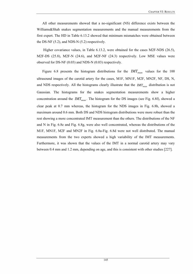
CHAPTER VI: RESULTS
All other measurements showed that a no-significant (NS) difference exists between the
Williams&Shah snakes segmentation measurements and the manual measurements from the
first expert. The HD in Table 6.13.2 showed that minimum mismatches were obtained between
the DS-NF (5.2), and NDS-N (5.2) respectively.
Higher covariance values, in Table 6.13.2, were obtained for the cases M2F-NDS (26.5),
M2F-DS (25.8), M2F-N (24.6), and M2F-NF (24.3) respectively. Low MSE values were
observed for DS-NF (0.03) and NDS-N (0.03) respectively.
Figure 6.8 presents the histogram distributions for the values for the 100
ultrasound images of the carotid artery for the cases, M1F, MN1F, M2F, MN2F, NF, DS, N,
and NDS respectively. All the histograms clearly illustrate that the distribution is not
Gaussian. The histograms for the snakes segmentation measurements show a higher
concentration around the . The histogram for the DS images (see Fig. 6.8f), showed a
clear peak at 0.7 mm whereas, the histogram for the NDS images in Fig. 6.8h, showed a
maximum around 0.6 mm. Both DS and NDS histogram distributions were more robust than the
rest showing a more concentrated IMT measurement than the others. The distributions of the NF
and N in Fig. 6.8e and Fig. 6.8g, were also well concentrated, whereas the distributions of the
M1F, MN1F, M2F and MN2F in Fig. 6.8a-Fig. 6.8d were not well distributed. The manual
measurements from the two experts showed a high variability of the IMT measurements.
Furthermore, it was shown that the values of the IMT in a normal carotid artery may vary
between 0.4 mm and 1.2 mm, depending on age, and this is consistent with other studies [227].
meanIMT
meanIMT
meanIMT
145
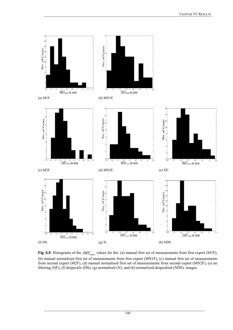
CHAPTER VI: RESULTS
(a) M1F. (b) MN1F.
(c) M2F. (d) MN2F. (e) NF.
(f) DS. (g) N. (h) NDS.
Fig. 6.8: Histograms of the values for the: (a) manual first set of measurements from first expert (M1F), (b) manual normalized first set of measurements from first expert (MN1F), (c) manual first set of measurements from second expert (M2F), (d) manual normalised first set of measurements from second expert (MN2F), (e) no filtering (NF), (f) despeckle (DS), (g) normalised (N), and (h) normalized despeckled (NDS), images.
meanIMT
146
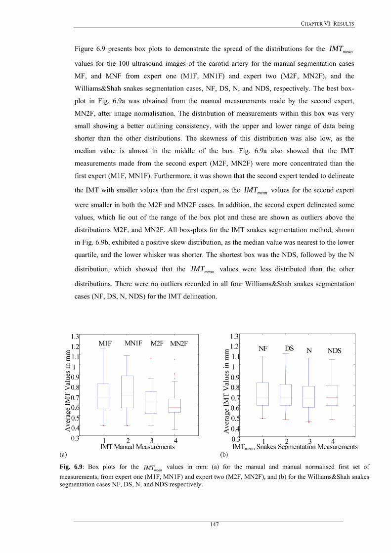
CHAPTER VI: RESULTS
Figure 6.9 presents box plots to demonstrate the spread of the distributions for the
values for the 100 ultrasound images of the carotid artery for the manual segmentation cases
MF, and MNF from expert one (M1F, MN1F) and expert two (M2F, MN2F), and the
Williams&Shah snakes segmentation cases, NF, DS, N, and NDS, respectively. The best box-
plot in Fig. 6.9a was obtained from the manual measurements made by the second expert,
MN2F, after image normalisation. The distribution of measurements within this box was very
small showing a better outlining consistency, with the upper and lower range of data being
shorter than the other distributions. The skewness of this distribution was also low, as the
median value is almost in the middle of the box. Fig. 6.9a also showed that the IMT
measurements made from the second expert (M2F, MN2F) were more concentrated than the
first expert (M1F, MN1F). Furthermore, it was shown that the second expert tended to delineate
the IMT with smaller values than the first expert, as the values for the second expert
were smaller in both the M2F and MN2F cases. In addition, the second expert delineated some
values, which lie out of the range of the box plot and these are shown as outliers above the
distributions M2F, and MN2F. All box-plots for the IMT snakes segmentation method, shown
in Fig. 6.9b, exhibited a positive skew distribution, as the median value was nearest to the lower
quartile, and the lower whisker was shorter. The shortest box was the NDS, followed by the N
distribution, which showed that the values were less distributed than the other
distributions. There were no outliers recorded in all four Williams&Shah snakes segmentation
cases (NF, DS, N, NDS) for the IMT delineation.
meanIMT
meanIMT
meanIMT
1 2 3 4 0.3 0.4 0.5 0.6 0.7 0.8 0.9 1 1.1 1.2 1.3
Ave
rage
IMT
Val
ues i
n m
m
IMT Manual Measurements
M1F MN1F M2F MN2F
1 2 3 40.3 0.4 0.50.60.7 0.80.9 11.1 1.21.3
Ave
rage
IMT
Val
ues
in m
m
IMTmean Snakes Segmentation Measurements
NF DS N NDS
(a) (b)
Fig. 6.9: Box plots for the values in mm: (a) for the manual and manual normalised first set of measurements, from expert one (M1F, MN1F) and expert two (M2F, MN2F), and (b) for the Williams&Shah snakes segmentation cases NF, DS, N, and NDS respectively.
meanIMT
147
CHAPTER VI: RESULTS
6.3.3 Regression and correlation analysis
The manual and the snakes segmented IMT borders were also compared using regression
and correlation analysis.
In order to further assess the inter-observer variability between the two experts, we have
plotted the manual segmentation results between the first and second expert, for the original
(M1F), and the normalized images (MN1F), on a regression plot with a least squares regression
line, as explained in section 5.7.4. Figure 6.10 shows scatter plots of the 100 measurements of
the measured by the two experts. In Fig. 6.10a the manual delineation results, M,
between the two experts on the original images are shown (M1F, M2F), whereas Fig. 6.10b
shows the manual delineation results, between the two experts, on the normalized images,
(MN1F, MN2F). It is shown from Fig. 6.10a that the first expert (Expert1), tended to give larger
measurements than the second expert (Expert 2). The manual measurements made by the two
experts on the original images (see Fig. 6.10a) resulted in a confidence interval limit of ±0.32
mm. However, when image normalization was used, the results of the two experts as shown in
Fig. 6.10b, were closer with a confidence interval limit of ±0.26 mm. Furthermore, the plotted
points in Fig. 6.10b were closer to the ideal regression line, and more evenly distributed on both
sides of it.
meanIMT
(a) 32.068.0 ±=y , 79.0=x . (b) 26.062.0 ±=y , 76.0=x .
Fig. 6.10: A scatter plot with least squares regression line for the inter-observer variability of the manual IMT delineation between the two experts for 100 ultrasound images of the carotid artery, on: (a) the original (M), and (b) the normalised (MN) images.
Table 6.14 presents the results of the Pearson correlation and the correlation coefficient
between the different snakes segmentation methods. Higher Pearson correlation values,
illustrating stronger linear relationships, were observed for the NF-DS (0.98), NF-N (0.95), DS-
148

CHAPTER VI: RESULTS
N (0.95), DS-NDS (0.92), and N-NDS (0.91) images respectively. Low Pearson correlation
values were observed between the M1F-NDS (0.63), MN1F-NDS (0.66), M1F-NF (0.67), M1F-
DS (0.70), MN1F-NF (0.71), M1F-N (0.71), MN1F-DS (0.73) and MN1F-N (0.75)
respectively. In the right column of Table 6.14 higher values for the correlation coefficient were
obtained for the cases NF-DS (0.97), NF-N (0.93), DS-N (0.93), DS-NDS (0.92), N-NDS (0.91)
and NF-NDS (0.90) respectively.
TABLE 6.14 PEARSON CORRELATION TEST AND CORRELATION COEFFICIENT FOR THE 100 ULTRASOUND IMAGES OF THE CAROTID ARTERY. VALUES ABOVE 0.1654 SHOW SIGNIFICANT CORRELATION AT P<0.05. BOLDED
VALUES SHOW BEST PERFORMANCE.
Pearson Correlation Correlation Coefficient MN1F NF DS N NDS MN1F NF DS N NDS
M1F 0.90 0.67 0.70 0.71 0.63 0.88 0.59 0.62 0.63 0.63
MN1F 0.71 0.73 0.75 0.66 0.63 0.66 0.66 0.66
NF 0.98 0.95 0.90 0.97 0.93 0.90
DS 0.95 0.92 0.93 0.92
N 0.91 0.91 M1F: Manual first set of measurements from first expert, MN1F: Manual normalised first set of measurements from
first expert, NF: No filtering, DS: Despeckle, N: Normalised, NDS: Normalized despeckled.
Figure 6.11 presents the regression lines for the correlations between (a) the NF-M1F, (b)
NF-MN1F, (c) DS-MN1F, (d) N-MN1F, (e) NDS-MN1F, (f) DS-M1F, (g) N-M1F, and (h)
NDS-M1F IMT segmentation results. The best regression line plot was obtained for the N-
MN1F segmentation, as shown in Fig.6.11d, followed by the DS-MN1F in Fig. 6.11c, and the
N-M1F in Fig. 6.11g. The best correlation coefficient was obtained for the N-MN1F, in Fig.
6.11d, with a correlation coefficient of 75.0=ρ , a slope of 0.89 and an intercept of 0.10,
which differ significantly from one and zero respectively. The second best regression line was
given by the DS-MN1F segmentation, in Fig. 6.11c, with a correlation coefficient, 73.0=ρ , a
slope of 0.86 and an intercept of 0.11, whereas the third best regression plot was given for the
N-M1F, shown in Fig.6.11g, and the NF-MN1F shown in Fig. 6.11b, which exhibited a
correlation coefficient, 71.0=ρ , a slope of 0.84 and an intercept of 0.12, and 71.0=ρ , a
slope of 0.80 and an intercept of 0.15, respectively.
149
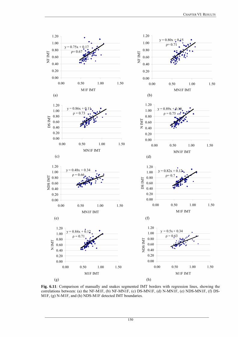
CHAPTER VI: RESULTS
y = 0.75x + 0.17ρ= 0.67
0.00
0.20
0.40
0.60
0.80
1.00
1.20
0.00 0.50 1.00 1.50
M1F IMT
NF
IMT
y = 0.80x + 0.15ρ= 0.71
0.00
0.20
0.40
0.60
0.80
1.00
1.20
0.00 0.50 1.00 1.50
MN1F IMT
NF
IMT
(a) (b)
y = 0.86x + 0.11ρ = 0.73
0.000.200.400.600.801.001.20
0.00 0.50 1.00 1.50
MN1F IMT
DS
IMT
y = 0.89x + 0.10ρ = 0.75
0.000.200.400.600.801.001.20
0.00 0.50 1.00 1.50
MN1F IMT
N IM
T
(c) (d)
y = 0.48x + 0.34ρ = 0.66
0.000.200.400.600.801.001.20
0.00 0.50 1.00 1.50
MN1F IMT
ND
S IM
T
y = 0.82x + 0.12ρ= 0.7
0.000.200.400.600.801.001.20
0.00 0.50 1.00 1.50
M1F IMT
DS
IMT
(e) (f)
y = 0.84x + 0.12ρ = 0.71
0.000.200.400.600.801.001.20
0.00 0.50 1.00 1.50
M1F IMT
N IM
T
y = 0.5x + 0.34ρ = 0.63
0.000.200.400.600.801.001.20
0.00 0.50 1.00 1.50
M1F IMT
ND
S IM
T
(g) (h)
Fig. 6.11: Comparison of manually and snakes segmented IMT borders with regression lines, showing the correlations between: (a) the NF-M1F, (b) NF-MN1F, (c) DS-MN1F, (d) N-MN1F, (e) NDS-MN1F, (f) DS-M1F, (g) N-M1F, and (h) NDS-M1F detected IMT boundaries.
150
CHAPTER VI: RESULTS
More useful information about the IMT segmentation accuracy, than the correlation plots,
can be obtained by plotting a Bland-Altman plot, described in Chapter 5.7.4, of the manual
versus the Williams&Shah snakes segmentation results. The Bland-Altman test may also be
used when assessing reproducibility. Figure 6.12 illustrates the Bland-Altman plots for different
combinations of the manual and snakes segmentation methods investigated. For both experts the
best plots were obtained for the NDS images (see Fig. 6.12m, n, o, p), where the difference with
the segmentation method for the manual measurements ± the standard deviation of the first
expert, M1F, is 0.02±0.25 (see Fig. 6.12m), and for the manual measurements of the second
expert, M2F, is –0.01±0.33 (see Fig. 6.12o).
151
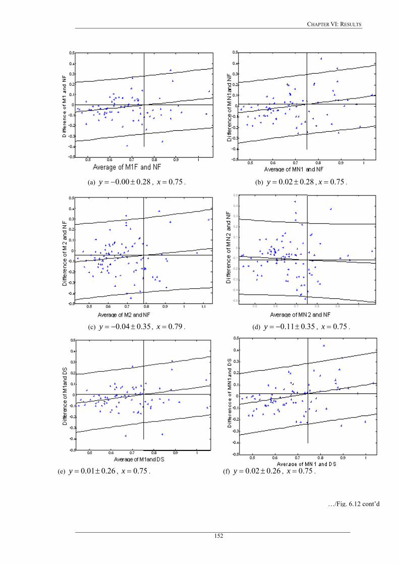
CHAPTER VI: RESULTS
(a) , . 28.000.0 ±−=y 75.0=x (b) 28.002.0 ±=y , . 75.0=x
(c) , . 35.004.0 ±−=y 79.0=x (d) 35.011.0 ±−=y , . 75.0=x
(e) , . 26.001.0 ±=y 75.0=x (f) 26.002.0 ±=y , . 75.0=x
…/Fig. 6.12 cont’d
152
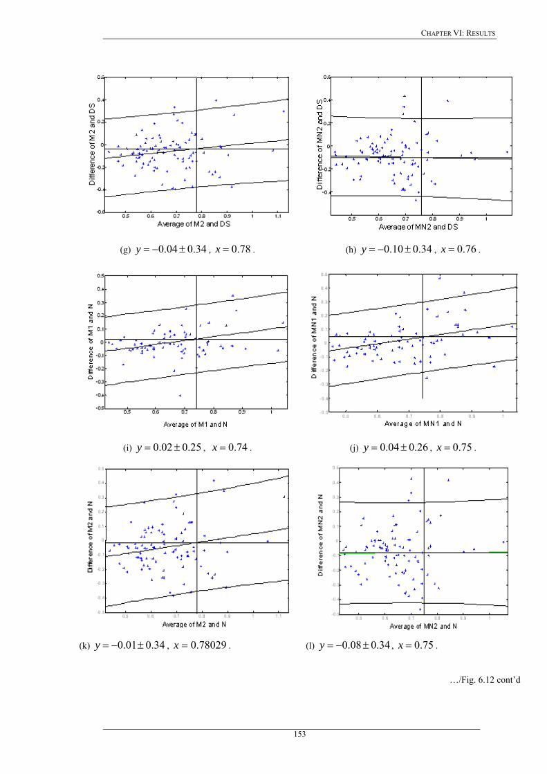
CHAPTER VI: RESULTS
(g) , . 34.004.0 ±−=y 78.0=x (h) 34.010.0 ±−=y , . 76.0=x
(i) , . 25.002.0 ±=y 74.0=x (j) 26.004.0 ±=y , . 75.0=x
(k) , . 34.001.0 ±−=y 78029.0=x (l) 34.008.0 ±−=y , . 75.0=x
…/Fig. 6.12 cont’d
153

CHAPTER VI: RESULTS
(m) , . 25.002.0 ±=y 74.0=x (n) 25.003.0 ±=y , . 73.0=x
(o) , . 33.001.0 ±−=y 77.0=x (p) 32.008.0 ±−=y , . 74.0=x
Fig. 6.12: Regression lines (Bland-Altman plots) of manual versus Williams&Shah snakes segmentation method for the for the first set of measurements for both experts. The middle line represents the mean difference, and the
upper and lower two outside lines represent the limits of agreement between the two methods, which are the mean of the data for the estimated difference between the two methods.
meanIMT
sd2±
154
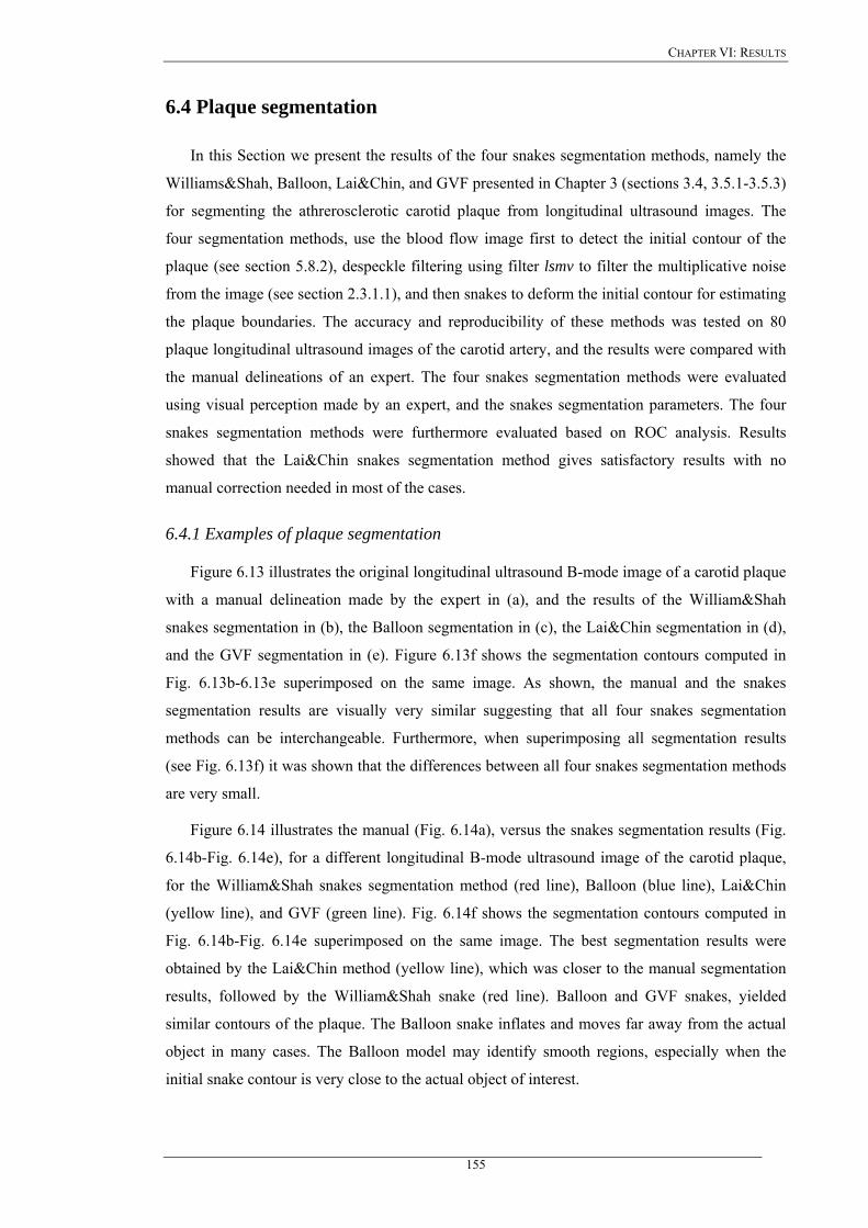
CHAPTER VI: RESULTS
6.4 Plaque segmentation
In this Section we present the results of the four snakes segmentation methods, namely the
Williams&Shah, Balloon, Lai&Chin, and GVF presented in Chapter 3 (sections 3.4, 3.5.1-3.5.3)
for segmenting the athrerosclerotic carotid plaque from longitudinal ultrasound images. The
four segmentation methods, use the blood flow image first to detect the initial contour of the
plaque (see section 5.8.2), despeckle filtering using filter lsmv to filter the multiplicative noise
from the image (see section 2.3.1.1), and then snakes to deform the initial contour for estimating
the plaque boundaries. The accuracy and reproducibility of these methods was tested on 80
plaque longitudinal ultrasound images of the carotid artery, and the results were compared with
the manual delineations of an expert. The four snakes segmentation methods were evaluated
using visual perception made by an expert, and the snakes segmentation parameters. The four
snakes segmentation methods were furthermore evaluated based on ROC analysis. Results
showed that the Lai&Chin snakes segmentation method gives satisfactory results with no
manual correction needed in most of the cases.
6.4.1 Examples of plaque segmentation
Figure 6.13 illustrates the original longitudinal ultrasound B-mode image of a carotid plaque
with a manual delineation made by the expert in (a), and the results of the William&Shah
snakes segmentation in (b), the Balloon segmentation in (c), the Lai&Chin segmentation in (d),
and the GVF segmentation in (e). Figure 6.13f shows the segmentation contours computed in
Fig. 6.13b-6.13e superimposed on the same image. As shown, the manual and the snakes
segmentation results are visually very similar suggesting that all four snakes segmentation
methods can be interchangeable. Furthermore, when superimposing all segmentation results
(see Fig. 6.13f) it was shown that the differences between all four snakes segmentation methods
are very small.
Figure 6.14 illustrates the manual (Fig. 6.14a), versus the snakes segmentation results (Fig.
6.14b-Fig. 6.14e), for a different longitudinal B-mode ultrasound image of the carotid plaque,
for the William&Shah snakes segmentation method (red line), Balloon (blue line), Lai&Chin
(yellow line), and GVF (green line). Fig. 6.14f shows the segmentation contours computed in
Fig. 6.14b-Fig. 6.14e superimposed on the same image. The best segmentation results were
obtained by the Lai&Chin method (yellow line), which was closer to the manual segmentation
results, followed by the William&Shah snake (red line). Balloon and GVF snakes, yielded
similar contours of the plaque. The Balloon snake inflates and moves far away from the actual
object in many cases. The Balloon model may identify smooth regions, especially when the
initial snake contour is very close to the actual object of interest.
155
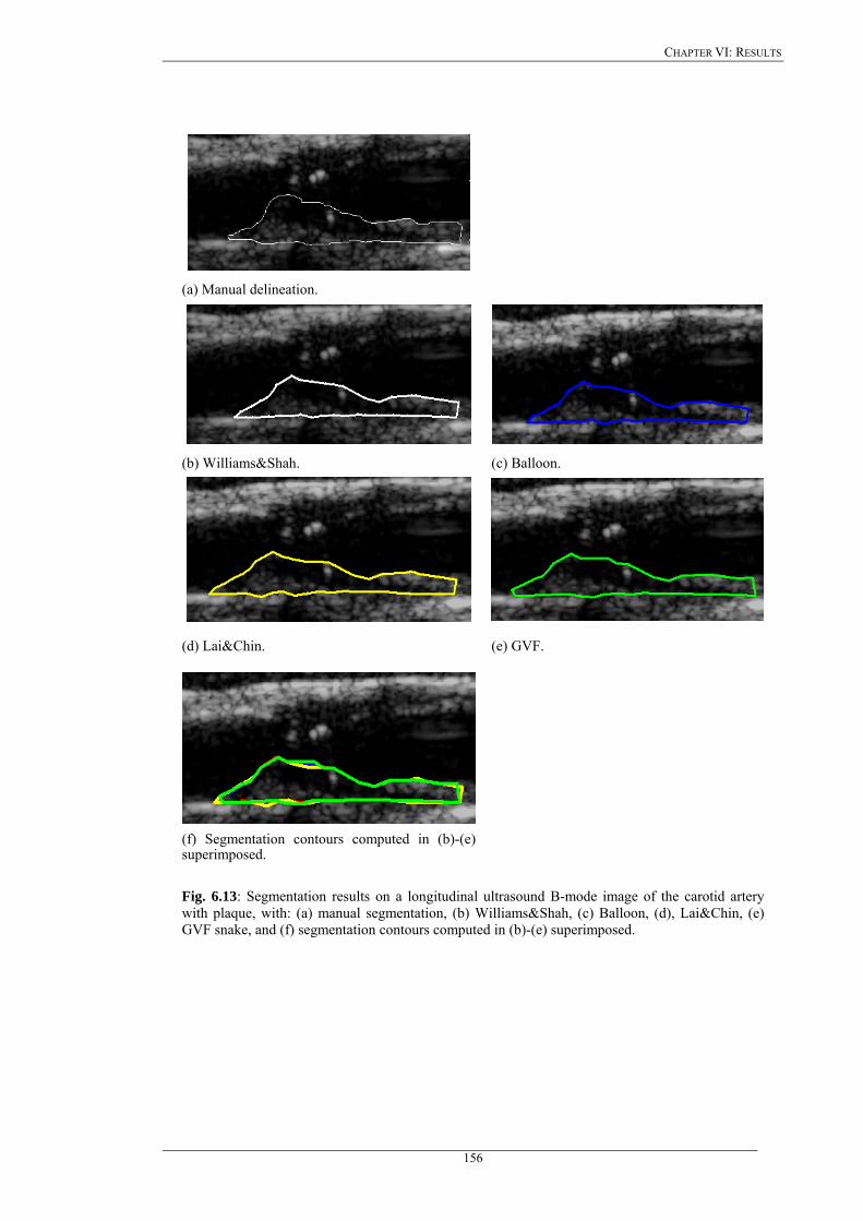
CHAPTER VI: RESULTS
(a) Manual delineation.
(b) Williams&Shah. (c) Balloon.
(d) Lai&Chin. (e) GVF.
(f) Segmentation contours computed in (b)-(e) superimposed.
Fig. 6.13: Segmentation results on a longitudinal ultrasound B-mode image of the carotid artery with plaque, with: (a) manual segmentation, (b) Williams&Shah, (c) Balloon, (d), Lai&Chin, (e) GVF snake, and (f) segmentation contours computed in (b)-(e) superimposed.
156

CHAPTER VI: RESULTS
(a) Manual delineation.
(b) Williams&Shah. (c) Balloon.
(d) Lai&Chin. (e) GVF.
(f) Segmentation contours computed in (b)-(e) superimposed.
Fig. 6.14: Segmentation results on a longitudinal ultrasound B-mode image of the carotid artery with plaque, with: (a) manual segmentation, (b) Williams&Shah, (c) Balloon, (d), Lai&Chin, (e) GVF snake, and (f) all segmentation contours computed in (b)-(e) superimposed.
157
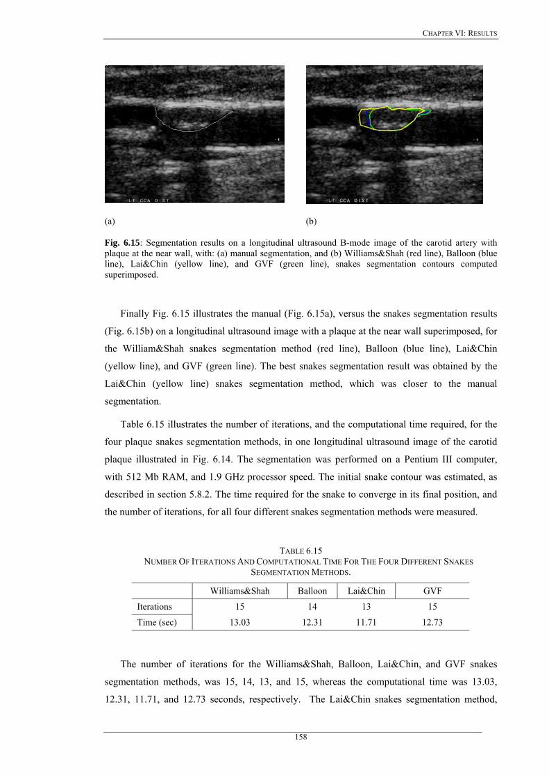
CHAPTER VI: RESULTS
(a) (b)
Fig. 6.15: Segmentation results on a longitudinal ultrasound B-mode image of the carotid artery with plaque at the near wall, with: (a) manual segmentation, and (b) Williams&Shah (red line), Balloon (blue line), Lai&Chin (yellow line), and GVF (green line), snakes segmentation contours computed superimposed.
Finally Fig. 6.15 illustrates the manual (Fig. 6.15a), versus the snakes segmentation results
(Fig. 6.15b) on a longitudinal ultrasound image with a plaque at the near wall superimposed, for
the William&Shah snakes segmentation method (red line), Balloon (blue line), Lai&Chin
(yellow line), and GVF (green line). The best snakes segmentation result was obtained by the
Lai&Chin (yellow line) snakes segmentation method, which was closer to the manual
segmentation.
Table 6.15 illustrates the number of iterations, and the computational time required, for the
four plaque snakes segmentation methods, in one longitudinal ultrasound image of the carotid
plaque illustrated in Fig. 6.14. The segmentation was performed on a Pentium III computer,
with 512 Mb RAM, and 1.9 GHz processor speed. The initial snake contour was estimated, as
described in section 5.8.2. The time required for the snake to converge in its final position, and
the number of iterations, for all four different snakes segmentation methods were measured.
TABLE 6.15 NUMBER OF ITERATIONS AND COMPUTATIONAL TIME FOR THE FOUR DIFFERENT SNAKES
SEGMENTATION METHODS.
Williams&Shah Balloon Lai&Chin GVF
Iterations 15 14 13 15
Time (sec) 13.03 12.31 11.71 12.73
The number of iterations for the Williams&Shah, Balloon, Lai&Chin, and GVF snakes
segmentation methods, was 15, 14, 13, and 15, whereas the computational time was 13.03,
12.31, 11.71, and 12.73 seconds, respectively. The Lai&Chin snakes segmentation method,
158
CHAPTER VI: RESULTS
exhibited the lower computational time (11.71 sec), and smaller number of iterations (13
iterations). The Balloon method, exhibited a larger number of iterations (14), and computational
time (12.31 sec), the Williams&Shah run at 15 iterations and 13.03 sec and the GVF run at 15
iterations and 12.73 sec. Table 6.15 also showed that on average a relative small number of
iterations and a low computational time was required for all four snakes segmentation methods,
and this is due to the snake initialisation procedure, proposed in Chapter 5.8.2, with which the
initial snake contour is placed close to the area of interest.
1.00001.00011.00021.00031.00041.00051.00061.0007
0 5 10 15 20
Iterations
TSEP
0.7280.7300.7320.7340.7360.7380.740
0 5 10 15
IterarionsTS
EB
(a) Williams&Shah TSEP. (b) Balloon TSEB.
1.0001.0001.0001.0001.0011.0011.0011.0011.0011.002
0 5 10 15 20
Iterations
TSEL
C
0.8800.9000.9200.9400.9600.9801.0001.020
0 5 10 15
Iterations
TSEG
VF
(c) Lai&Chin TSELC. (d) GVF TSEGVF.
Fig. 6.16: Plots of the total snake energy for: (a) the Williams&Shah (TSEP), (b) Balloon (TSEB), (c) Lai&Chin (TSELC), and (d) GVF snake (TSEGVF) for the image in Fig. 6.14a.
159
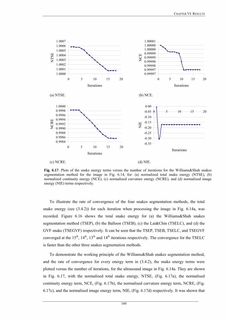
CHAPTER VI: RESULTS
1.00001.00011.00021.00031.00041.00051.00061.0007
0 5 10 15 20
Iterations
NTS
E
0.999970.999970.999980.999980.999990.999991.000001.000001.00001
0 5 10 15 20
Iterations
NC
E
(a) NTSE. (b) NCE.
0.99840.99860.99880.99900.99920.99940.99960.99981.0000
0 5 10 15 20
Iterations
NC
RE
-0.35-0.30-0.25-0.20-0.15-0.10-0.050.00
0 5 10 15 20
Iterarions
NIE
(c) NCRE. (d) NIE.
Fig. 6.17: Plots of the snake energy terms versus the number of iterations for the Williams&Shah snakes segmentation method for the image in Fig. 6.14, for: (a) normalized total snake energy (NTSE), (b) normalized continuity energy (NCE), (c) normalized curvature energy (NCRE), and (d) normalized image energy (NIE) terms respectively.
To illustrate the rate of convergence of the four snakes segmentation methods, the total
snake energy (see (3.4.2)) for each iteration when processing the image in Fig. 6.14a, was
recorded. Figure 6.16 shows the total snake energy for (a) the Williams&Shah snakes
segmentation method (TSEP), (b) the Balloon (TSEB), (c) the Lai&Chin (TSELC), and (d) the
GVF snake (TSEGVF) respectively. It can be seen that the TSEP, TSEB, TSELC, and TSEGVF
converged at the 15th, 14th, 13th and 14th iterations respectively. The convergence for the TSELC
is faster than the other three snakes segmentation methods.
To demonstrate the working principle of the Williams&Shah snakes segmentation method,
and the rate of convergence for every energy term in (3.4.2), the snake energy terms were
plotted versus the number of iterations, for the ultrasound image in Fig. 6.14a. They are shown
in Fig. 6.17, with the normalised total snake energy, NTSE, (Fig. 6.17a), the normalised
continuity energy term, NCE, (Fig. 6.17b), the normalised curvature energy term, NCRE, (Fig.
6.17c), and the normalised image energy term, NIE, (Fig. 6.17d) respectively. It was shown that
160
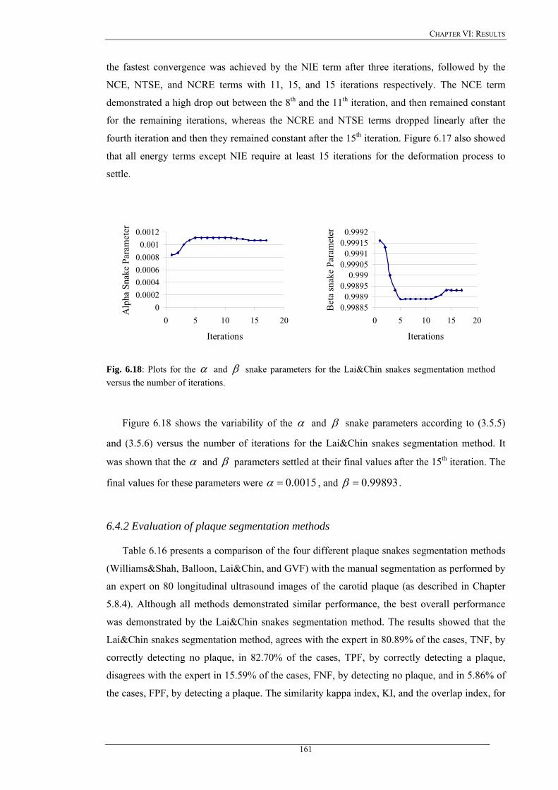
CHAPTER VI: RESULTS
the fastest convergence was achieved by the NIE term after three iterations, followed by the
NCE, NTSE, and NCRE terms with 11, 15, and 15 iterations respectively. The NCE term
demonstrated a high drop out between the 8th and the 11th iteration, and then remained constant
for the remaining iterations, whereas the NCRE and NTSE terms dropped linearly after the
fourth iteration and then they remained constant after the 15th iteration. Figure 6.17 also showed
that all energy terms except NIE require at least 15 iterations for the deformation process to
settle.
00.00020.00040.00060.00080.001
0.0012
0 5 10 15 20
Iterations
Alp
ha S
nake
Par
amet
er
0.998850.9989
0.998950.999
0.999050.9991
0.999150.9992
0 5 10 15 20
IterationsB
eta
snak
e Pa
ram
eter
Fig. 6.18: Plots for the α and β snake parameters for the Lai&Chin snakes segmentation method versus the number of iterations.
Figure 6.18 shows the variability of the α and β snake parameters according to (3.5.5)
and (3.5.6) versus the number of iterations for the Lai&Chin snakes segmentation method. It
was shown that the α and β parameters settled at their final values after the 15th iteration. The
final values for these parameters were 0015.0=α , and 99893.0=β .
6.4.2 Evaluation of plaque segmentation methods
Table 6.16 presents a comparison of the four different plaque snakes segmentation methods
(Williams&Shah, Balloon, Lai&Chin, and GVF) with the manual segmentation as performed by
an expert on 80 longitudinal ultrasound images of the carotid plaque (as described in Chapter
5.8.4). Although all methods demonstrated similar performance, the best overall performance
was demonstrated by the Lai&Chin snakes segmentation method. The results showed that the
Lai&Chin snakes segmentation method, agrees with the expert in 80.89% of the cases, TNF, by
correctly detecting no plaque, in 82.70% of the cases, TPF, by correctly detecting a plaque,
disagrees with the expert in 15.59% of the cases, FNF, by detecting no plaque, and in 5.86% of
the cases, FPF, by detecting a plaque. The similarity kappa index, KI, and the overlap index, for
161
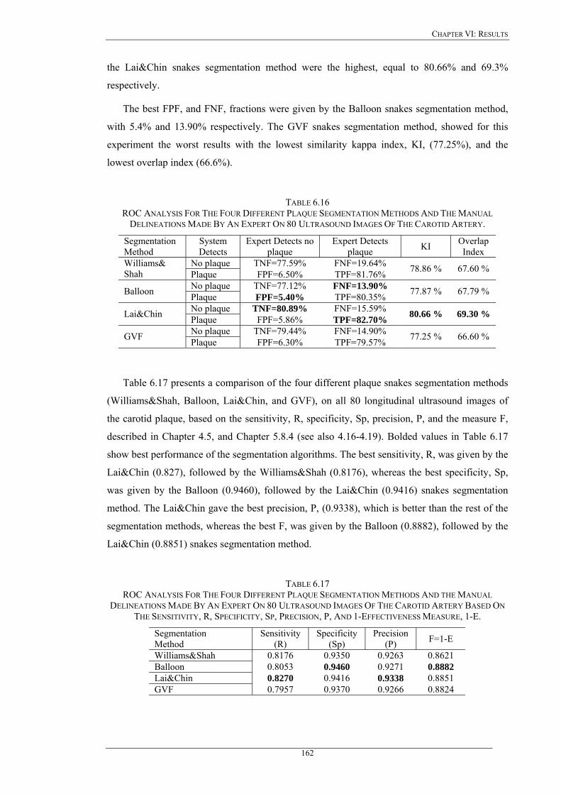
CHAPTER VI: RESULTS
the Lai&Chin snakes segmentation method were the highest, equal to 80.66% and 69.3%
respectively.
The best FPF, and FNF, fractions were given by the Balloon snakes segmentation method,
with 5.4% and 13.90% respectively. The GVF snakes segmentation method, showed for this
experiment the worst results with the lowest similarity kappa index, KI, (77.25%), and the
lowest overlap index (66.6%).
TABLE 6.16 ROC ANALYSIS FOR THE FOUR DIFFERENT PLAQUE SEGMENTATION METHODS AND THE MANUAL
DELINEATIONS MADE BY AN EXPERT ON 80 ULTRASOUND IMAGES OF THE CAROTID ARTERY.
Segmentation Method
System Detects
Expert Detects no plaque
Expert Detects plaque KI Overlap
Index No plaque TNF=77.59% FNF=19.64% Williams&
Shah Plaque FPF=6.50% TPF=81.76% 78.86 % 67.60 %
No plaque TNF=77.12% FNF=13.90% Balloon Plaque FPF=5.40% TPF=80.35% 77.87 % 67.79 %
No plaque TNF=80.89% FNF=15.59% Lai&Chin Plaque FPF=5.86% TPF=82.70% 80.66 % 69.30 %
No plaque TNF=79.44% FNF=14.90% GVF Plaque FPF=6.30% TPF=79.57% 77.25 % 66.60 %
Table 6.17 presents a comparison of the four different plaque snakes segmentation methods
(Williams&Shah, Balloon, Lai&Chin, and GVF), on all 80 longitudinal ultrasound images of
the carotid plaque, based on the sensitivity, R, specificity, Sp, precision, P, and the measure F,
described in Chapter 4.5, and Chapter 5.8.4 (see also 4.16-4.19). Bolded values in Table 6.17
show best performance of the segmentation algorithms. The best sensitivity, R, was given by the
Lai&Chin (0.827), followed by the Williams&Shah (0.8176), whereas the best specificity, Sp,
was given by the Balloon (0.9460), followed by the Lai&Chin (0.9416) snakes segmentation
method. The Lai&Chin gave the best precision, P, (0.9338), which is better than the rest of the
segmentation methods, whereas the best F, was given by the Balloon (0.8882), followed by the
Lai&Chin (0.8851) snakes segmentation method.
TABLE 6.17 ROC ANALYSIS FOR THE FOUR DIFFERENT PLAQUE SEGMENTATION METHODS AND THE MANUAL
DELINEATIONS MADE BY AN EXPERT ON 80 ULTRASOUND IMAGES OF THE CAROTID ARTERY BASED ON THE SENSITIVITY, R, SPECIFICITY, SP, PRECISION, P, AND 1-EFFECTIVENESS MEASURE, 1-E.
Segmentation Method
Sensitivity (R)
Specificity (Sp)
Precision (P) F=1-E
Williams&Shah 0.8176 0.9350 0.9263 0.8621 Balloon 0.8053 0.9460 0.9271 0.8882 Lai&Chin 0.8270 0.9416 0.9338 0.8851 GVF 0.7957 0.9370 0.9266 0.8824
162
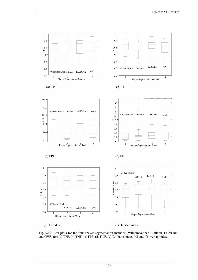
CHAPTER VI: RESULTS
1 2 3 4 0.4
0.5
0.6
0.7
0.8
0.9
1
TPF
Plaque Segmentation Method
Williams&Shah Balloon Lai&Chin GVF
1 2 3 4 0.4
0.5
0.6
0.7
0.8
0.9
1
TNF
Plaque Segmentation Method
Balloon Lai&Chin GVF Williams&Shah
(a) TPF. (b) TNF.
1 2 3 4 0
0.005
0.01
0.015
0.02
0.025
FPF
Plaque Segmentation Method
Williams&Shah Balloon Lai&Chin GVF
1 2 3 4 0
0.1
0.2
0.3
0.4
0.5
0.6
0.7
0.8
0.9
1
FNF
Plaque Segmentation Method
Williams&Shah Balloon Lai&Chin GVF
(c) FPF. (d) FNF.
1 2 3 4 0.4
0.5
0.6
0.7
0.8
0.9
1
KI i
ndex
Plaque Segmentation Method
Williams&Shah Balloon Lai&Chin GVF
1 2 3 4 0.4
0.5
0.6
0.7
0.8
0.9
1
Ove
rlap
inde
x
Plaque Segmentation Method
Williams&Shah Balloon Lai&Chin GVF
(e) KI index. (f) Overlap index.
Fig. 6.19: Box plots for the four snakes segmentation methods (Williams&Shah, Balloon, Lai&Chin, and GVF) for: (a) TPF, (b) TNF, (c) FPF, (d) FNF, (e) Williams index, KI and (f) overlap index.
163
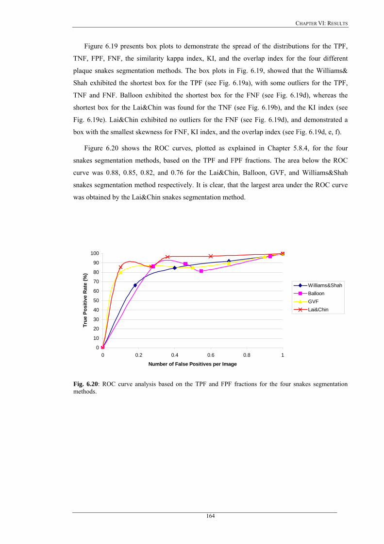
CHAPTER VI: RESULTS
Figure 6.19 presents box plots to demonstrate the spread of the distributions for the TPF,
TNF, FPF, FNF, the similarity kappa index, KI, and the overlap index for the four different
plaque snakes segmentation methods. The box plots in Fig. 6.19, showed that the Williams&
Shah exhibited the shortest box for the TPF (see Fig. 6.19a), with some outliers for the TPF,
TNF and FNF. Balloon exhibited the shortest box for the FNF (see Fig. 6.19d), whereas the
shortest box for the Lai&Chin was found for the TNF (see Fig. 6.19b), and the KI index (see
Fig. 6.19e). Lai&Chin exhibited no outliers for the FNF (see Fig. 6.19d), and demonstrated a
box with the smallest skewness for FNF, KI index, and the overlap index (see Fig. 6.19d, e, f).
Figure 6.20 shows the ROC curves, plotted as explained in Chapter 5.8.4, for the four
snakes segmentation methods, based on the TPF and FPF fractions. The area below the ROC
curve was 0.88, 0.85, 0.82, and 0.76 for the Lai&Chin, Balloon, GVF, and Williams&Shah
snakes segmentation method respectively. It is clear, that the largest area under the ROC curve
was obtained by the Lai&Chin snakes segmentation method.
0
10
20
30
40
50
60
70
80
90
100
0 0.2 0.4 0.6 0.8 1
Number of False Positives per Image
True
Pos
itive
Rat
e (%
)
Williams&ShahBalloonGVFLai&Chin
Fig. 6.20: ROC curve analysis based on the TPF and FPF fractions for the four snakes segmentation methods.
164

CHAPTER VII: DISCUSSION
Chapter 7
Discussion
165
CHAPTER VII: DISCUSSION
CHAPTER 7: DISCUSSION
In this work, we have presented a review for despeckling and segmentation techniques for
carotid ultrasound artery images. As a first task we have investigated the image quality of two
different ultrasound scanner models based on statistical and evaluation metrics. Furthermore we
have proposed despeckle filters that are more suitable for the despeckling of ultrasound images
of the carotid artery. Additionally, a snakes segmentation technique was proposed for
segmenting the IMT and the atherosclerotic carotid plaque from longitudinal ultrasound images.
A system was developed that is capable of despeckling and segmenting the IMT and plaque
borders in carotid artery ultrasound images, with better accuracy, and consistency compared
with the manual delineations from the experts. The system can delineate the borders
consistently, and thus enabling the expert to better and more accurately evaluate the risk of
stroke. The aim of the system is not to entirely replace the manual delineations but to
complement the experts manual evaluation.
7.1 Image quality evaluation of two ultrasound scanners
Image quality is very important in the assessment of atherosclerosis and the evaluation of
the risk of stroke in ultrasound imaging. We have therefore, evaluated two different ultrasound
scanners (ATL HDI-3000, and ATL HDI-5000) on 80 longitudinal ultrasound images of the
carotid artery bifurcation, before and after despeckle filtering, after normalization, and after
despeckle filtering and normalization. The evaluation was based on visual evaluation by two
experts, despeckle filtering, statistical and texture features, as well as based on image quality
evaluation metrics. It should be noted that there are no other studies found in the literature for
comparing the performance of the two ultrasound scanners.
7.1.1 Visual perception
It is clearly shown that the ATL HDI-5000 scanner produces images with higher quality. It
was also shown that despeckle filtering and normalisation produces better images (see Fig. 6.1,
Fig. 6.2, Table 6.1). Normalisation was also proposed in other studies using blood echogenicity
as a reference and applied in carotid artery images [93], [235]. In [322], it was shown that
normalisation improves the image compatibility by reducing the variability introduced by
different gain settings, different operators, and different equipment.
7.1.2 Statistical and texture measures
Some statistical measures, as shown in the first part of Table 6.2, were better after
normalization, and some others, shown in the second part of Table 6.2, were better after
despeckle filtering. Table 6.2 also showed that the contrast was higher for the NF and N images
166
CHAPTER VII: DISCUSSION
on both scanners. All other measures presented in Table 6.2 are comparable showing that better
values were obtained on the NDS images. Moreover it was shown that the entropy that is a
measure of the information content of the image [128] was higher for both scanners in the cases
of the NDS and DS images. Low entropy images have low contrast and large areas of pixels
with same or similar gray level values. An image which is perfectly uniform will have a zero
entropy. On the other hand, high entropy images have high contrast and thus higher entropy
values [3]. The ATL HDI-5000 scanner produces therefore images with higher information
content. The entropy was also used in other studies to classify the best liver ultrasound images
[211], where it was shown that the experts rate images with higher entropy values better. In [10]
entropy was used to classify between symptomatic and asymptomatic carotid plaques. Finally in
[147] higher entropy values indicated a higher probability of a cloud to give rain.
7.1.3 Quality evaluation metrics
Marginal differences were observed from Table 6.3 between the ATL HDI-3000 and the
ATL HDI-5000 scanner. For example, the MSE and the RMSE remained almost the same for
both scanners. It was documented in [272], [278], [279], [283], [289], that the MSE, RMSE,
SNR and PSNR, are not objective measures for image quality evaluation nor do they correspond
to all aspects of the visual perception. Furthermore, they do not correctly reflect artifacts [284],
[289], [300]. While MSE and RMSE values were in the range of 0.4 to 2.0, for all cases, Err3,
Err4, SNR, PSNR, Q, and SSIN were significantly better on the NF-N images for both scanners,
showing that normalization increases the values of these measures. Using the recently proposed
measures for objective image evaluation Q [272], and SSIN [278], the best performance for both
scanners was given by the NF-N. The values for Q and SSIN for both scanners on the NF-N
images were 0.95 and 0.95 respectively. These results were followed with Q=0.73, and
SSIN=0.92 in the case of NF-NDS for the HDI ATL-3000 scanner, and Q=0.72, and SSIN=0.94
in the case of NF-DS for the HDI ATL-5000 scanner. It is noted that the findings of the image
quality evaluation metrics showed that the best results were obtained on the NF-N and NF-NDS
images, whereas the visual perception evaluation (see Table 6.1) showed that best results were
obtained for the NDS and DS images.
The results of this study showed that normalization and despeckle filtering are an important
procedure favouring image quality, and should be further investigated.
7.1.4 Summary findings on image quality evaluation
Table 7.1 summarises the image quality evaluation results of this study, for the visual
evaluation (Table 6.1), the statistical and texture analysis (Table 6.2), and the image quality
evaluation metrics (Table 6.3), as presented in Chapter 6.1. A double plus sign in Table 7.1
167
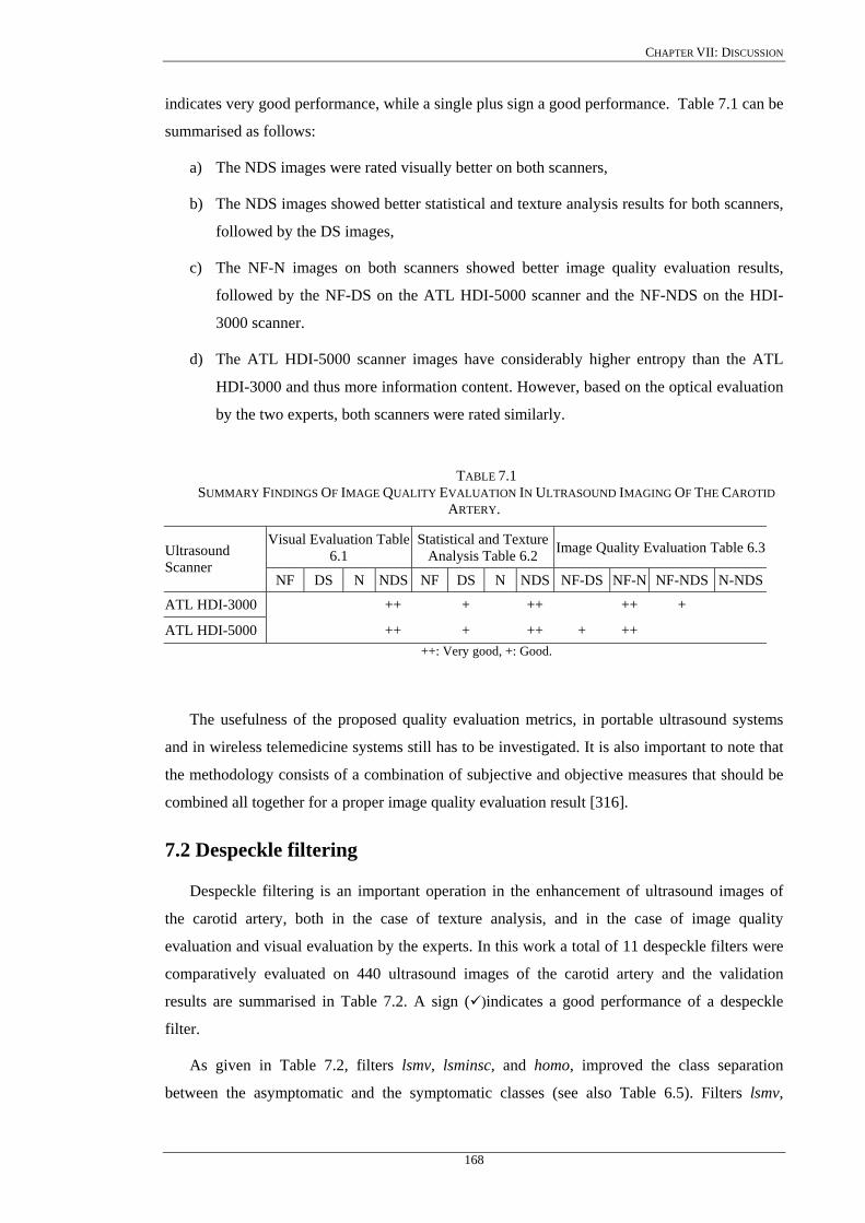
CHAPTER VII: DISCUSSION
indicates very good performance, while a single plus sign a good performance. Table 7.1 can be
summarised as follows:
a) The NDS images were rated visually better on both scanners,
b) The NDS images showed better statistical and texture analysis results for both scanners,
followed by the DS images,
c) The NF-N images on both scanners showed better image quality evaluation results,
followed by the NF-DS on the ATL HDI-5000 scanner and the NF-NDS on the HDI-
3000 scanner.
d) The ATL HDI-5000 scanner images have considerably higher entropy than the ATL
HDI-3000 and thus more information content. However, based on the optical evaluation
by the two experts, both scanners were rated similarly.
TABLE 7.1 SUMMARY FINDINGS OF IMAGE QUALITY EVALUATION IN ULTRASOUND IMAGING OF THE CAROTID
ARTERY.
Visual Evaluation Table 6.1
Statistical and Texture Analysis Table 6.2 Image Quality Evaluation Table 6.3Ultrasound
Scanner NF DS N NDS NF DS N NDS NF-DS NF-N NF-NDS N-NDS
ATL HDI-3000 ++ + ++ ++ +
ATL HDI-5000 ++ + ++ + ++ ++: Very good, +: Good.
The usefulness of the proposed quality evaluation metrics, in portable ultrasound systems
and in wireless telemedicine systems still has to be investigated. It is also important to note that
the methodology consists of a combination of subjective and objective measures that should be
combined all together for a proper image quality evaluation result [316].
7.2 Despeckle filtering
Despeckle filtering is an important operation in the enhancement of ultrasound images of
the carotid artery, both in the case of texture analysis, and in the case of image quality
evaluation and visual evaluation by the experts. In this work a total of 11 despeckle filters were
comparatively evaluated on 440 ultrasound images of the carotid artery and the validation
results are summarised in Table 7.2. A sign ( )indicates a good performance of a despeckle
filter.
As given in Table 7.2, filters lsmv, lsminsc, and homo, improved the class separation
between the asymptomatic and the symptomatic classes (see also Table 6.5). Filters lsmv,
168

CHAPTER VII: DISCUSSION
lsminsc, and gf4d gave a high number of significantly different features (see Table 6.6). Filters
lsminsc, gf4d, and homo, gave only a marginal improvement in the percentage of correct
classifications success rate (see Table 6.7). Moreover, filters lsmv, nldif, and waveltc, gave
better image quality evaluation results (see Table 6.8). Filters lsmv, and gf4d, improved the
visual assessment carried out by the experts (see Table 6.91, Table 6.9.2)). It is clearly shown
that filter lsmv gave the best performance, followed by filters lsminsc, and gf4d (see Table 7.2).
Filter lsmv or gf4d can be used for despeckling asymptomatic images where the expert is
interested mainly in the plaque composition and texture analysis. Filters lsmv or gf4d or lsminsc
can be used for despeckling of symptomatic images where the expert is interested in identifying
the degree of stenosis and the plaque borders. Filters homo, nldif, and waveltc gave poorer
performance.
TABLE 7.2 SUMMARY FINDINGS OF DESPECKLE FILTERING IN ULTRASOUND IMAGING OF THE CAROTID ARTERY.
Despeckle Filter Statistical and
Texture Features Table 6.5
Statistical Analysis Table 6.6
kNN Classifier Table 6.7
Image Quality Evaluation Table 6.8
Optical Perception Evaluation Table 6.9.1, Table 6.9.2
Local Statistics lsmv lsminsc Geometric Filtering gf4d Homomorphic Filtering homo Diffusion Filtering nldif Wavelet Filtering waveltc
: Indicates good performance of a despeckle filter.
7.2.1 Despeckle filtering on an artificial and a real carotid image
Figure 6.3 and Fig. 6.5 showed that good optical results were obtained by the despeckle
filters lsmv (Fig. 6.3b, Fig. 6.5b), lsminsc (Fig. 6.3c, Fig. 6.5c), and gf4d (Fig. 6.3h, Fig. 6.5h).
The lsmv removed the noise around the IMT, and thus the borders between IMT and blood were
more easily identified. Moreover, it was shown from the line profile in Fig. 6.4b, that both the
edge and the locality of boundaries were well preserved by the lsmv despeckle filter. The
lsminsc shown in Fig. 6.3c, and Fig. 6.5c performed a textural orientation on the image,
grouping the homogeneous areas together. This is good especially when applying the filter on
plaque areas, as the plaque borders will be kept together. It was also shown from Fig. 6.4c, that
169
CHAPTER VII: DISCUSSION
boundaries were well preserved for the filter lsminsc although some noise still remained after
despeckle filtering. The images in Fig. 6.3h, and Fig. 6.5h, which were processed by the gf4d,
were brighter after filtering, and the borders of the IMT were well recognized. Figure 6.4h
showed that boundaries were also well preserved where some noise remained on edges. Finally
the filter nldif, preserved the boundaries (Fig. 6.3k), but a lot of noise remained after filtering
(Fig. 6.4k).
The rest of the images in Fig. 6.3 and Fig. 6.5, showed a blurring effect (Fig. 6.3d-g, i, j, l),
edges were not well preserved (Fig. 6.3d-g, j, l), the image became darker after filtering (Fig.
6.3i), and homogeneous areas were blurred (Fig. 6.3d-g, i, j, l). The line profiles of the
despeckle filters, median, wiener, ls, homog, homo, ad, nldif, and waveltc, in Fig. 6.4 showed
that a substantial noise component remained after filtering (Fig. 6.4i,k), and that the locality of
boundaries were not well preserved (Fig. 6.4d-g, i-l).
The results in Table 6.4, showed that the gf4d, increases enormously the contrast, followed
by homo, and lsminsc, where the lsmv, gf4d and lsminsc reduces the speckle index, C,
considerably. The contrast-to-speckle radio, CSR, was very good for the filter homo, followed
by the gf4d, and lsminsc.
Despeckle filtering was investigated by other researchers and also in our study, on an
artificial carotid image (Fig. 6.3), [38], on line profiles (Fig. 6.4) of different ultrasound images,
[175], [326], [345], [349], and real longitudinal ultrasound images of the carotid artery (Fig.
6.5) [38]. There is only one study [38], where despeckle filtering was investigated on one real,
and one artificial longitudinal ultrasound image of the carotid artery. Four different despeckle
filters were applied in [38], namely the Lee [22], Frost [27], anisotropic diffusion [347], and a
speckle reducing anisotropic diffusion filter [38]. The despeckle window used for the Lee, and
Frost filters was 7x7 pixels. To evaluate the performance of these filters, the mean and the
standard deviation were used, which were calculated in different regions of the carotid artery
image, namely in lumen, tissue, and at the vascular wall. The mean gray level values of the
original image for the lumen, tissue and wall regions were 1.03, 5.31, and 22.8, whereas the
variance were 0.56, 2.69, and 10.61. The mean after despeckle filtering with the speckle
anisotropic diffusion gave brighter values for the lumen and tissue. Specifically the mean for the
lumen, tissue, and wall for the speckle reducing anisotropic diffusion was (1.19, 6.17, 18.9), Lee
(1.11, 5.72, 21.75), Frost (1.12, 5.74, 21.83) and anisotropic diffusion (0.90, 4.64, 14.64). The
standard deviation for the speckle anisotropic diffusion gave lower values (0.15, 0.7, 2.86) when
compared with Lee (0.33, 1.42, 5.37), Frost (0.32, 1.40, 5.30), and anisotropic diffusion (0.20,
1.09, 3.52). It was thus shown that the speckle reducing anisotropic diffusion filter preserves the
mean and reduces the variance. The number of images investigated in [38], was very small,
visual perception evaluation by experts was not carried out, as well as only two statistical
170

CHAPTER VII: DISCUSSION
measures were used to quantitatively evaluate despeckle filtering, namely the mean, and the
variance before and after despeckle filtering as explained above. We believe that the mean and
the variance used in [38] are not indicative and may not give a complete, and accurate
evaluation result. Furthermore, despeckle filtering was investigated by other researchers on
ultrasound images of, heart [345], pig heart [349], pig muscle [75], [76], kidney [141], liver
[271], echocardiograms [348], CT lung scans [37], MRI images of brain [124], [228], [344],
brain X-ray images [326], SAR images [38], [88], [91], [92], [98], [107], [229], and real world
images [285].
Line plots, as used in our study (see Fig. 6.4), were also used in few other studies to quantify
despeckle filtering performance. Specifically in [326], a line profile through the original and the
despeckled ultrasound image of kidney was plotted, using adaptive Gaussian filtering. In [186]
line profiles were plotted on four simulated and 15 ultrasound cardiac images of the left
ventricle, in order to evaluate median filtering. In another study [345], line profiles through one
phantom, one heart, one kidney, and one liver ultrasound image, were plotted where an adaptive
shrinkage weighted median [271], [285], wavelet shrinkage [350], and wavelet shrinkage
coherence enhancing [348] models were used and compared with a non linear coherent
diffusion model [345]. Finally in [349], line plots were used in one artificial computer simulated
image, and one ultrasound image of pig heart, where an adaptive shrinkage weighted median
filter [271], a multiscale nonlinear thresholding without adaptive filter pre-processing [349], a
wavelet shrinkage filtering method [350], and a proposed adaptive nonlinear thresholding with
adaptive pre-processing method [349], were evaluated. In all above studies, visual perception
evaluation by experts, statistical and texture analysis, on multiple images, as performed in our
study, was not performed.
7.2.2 Texture analysis
The results on texture analysis, presented in Chapter 6.2.2 (Table 6.5-Table 6.7), showed
that the filters lsmv, gf4d, and lsminsc (Table 7.2), improved the class separation between the
asymptomatic and the symptomatic classes (Table 6.5), by increasing the distance between
them. These filters, lsmv, gf4d, and lsminsc, gave the highest number of significantly different
features (Table 6.6), with 7, 6, and 5 respectively, and gave only a marginal improvement in the
percentage of correct classification success rate (Table 6.7). The high number of significantly
different features for these filters, showed that the two classes (asymptomatic, symptomatic),
may be better separated after despeckle filtering with the filters lsmv, gf4d, and lsminsc. Table
6.5 showed that almost all despeckle filters increased the distance between the asymptomatic
and the symptomatic images thus making the identification of a class more easily to identify.
Table 6.5 also showed that most of the filters reduced the asymmetry, , and the skewness,
, of the histogram. Table 6.6 showed, that despeckle filtering influenced more some
3σ4σ
171
CHAPTER VII: DISCUSSION
statistical features, such as the inverse difference moment, IDM, the angular second moment,
ASM, and the sum entropy, , while other statistical features were less influenced by
despeckle filtering. As a result, these features, which were more influenced, may be used in
future research to evaluate despeckle filtering. The in the last row of Table
6.5, showed that best feature distance was given by the filters homo, lsminsc, median, and lsmv.
Table 6.7 showed that not all feature sets equally benefited from despeckle filtering.
Specifically, the SF and TEM feature sets benefited from almost all despeckle filters (7),
whereas the feature sets SGLDMm, GLDS, and NGTDM, benefited from four despeckle filters,
FDTA three and SFM two. The features sets SGLDMr, and FPS, benefited from only one
despeckle filter.
∑Entr
TDisScore __
There were some results given in the recent literature based on texture analysis of ultrasound
images for, the classification of atherosclerotic carotid plaque [10], [48], [127], [138], [139],
liver ultrasound images [211], [236], electron microscopic muscle images [171], detection of
breast masses [232], cloud images [147], SAR images [31], and some results given on artificial
images from the pioneer researchers in texture analysis [128], [129]. There is no other study
reported in the literature, where texture analysis (Table 6.5-Table 6.7) was used to the extent,
that is used in our study, to evaluate despeckle filtering in ultrasound imaging. In studies [10],
[48], [127], some of the texture measures used in our study (Table 6.5), were also used on a
total of 230 ultrasound images of the carotid plaque (115 asymptomatic, 115 symptomatic), in
order to characterise carotid plaques as safe or unsafe and identify patients at risk of stroke.
Specifically in [10], and [148] all nine different features used in our study (see Table 6.7) were
also used to classify a plaque as asymptomatic or symptomatic, where comparable values as in
our study were obtained for all feature sets. Examples of the use of texture analysis were also
provided in [232], for classifying malignant and benign tumours of breast, in [147] for
classifying clouds and predicting weather, and finally in [129] to automatically classify terrain
texture.
7.2.3 Image quality evaluation metrics
The image quality evaluation results presented in Table 6.8 showed that the best values were
obtained by the despeckle filters nldif, lsmv, and waveltc. It was shown from Table 6.8, that the
effect of despeckle filtering was more obvious on the asymptomatic images, where generally
better image quality evaluation results were obtained. Moreover, it is obvious that all quality
evaluation metrics presented here were equally important for image quality evaluation. It is
furthermore important to note that a higher PSNR (or equivalently, a lower RMSE) does not
necessarily imply a higher subjective image quality, although they do provide some measure of
relative quality. While some quality metrics for different images have been studied and
172
CHAPTER VII: DISCUSSION
proposed in the literature, such as for MRI [273], natural and artificial images [272], [278],
[286], to the best of our knowledge, no other comparative study exists that have investigated the
application of the above metrics together with visual perception evaluation, on ultrasound
images of the carotid artery. In previous studies [131], [160], [174], [181], [238], [272], [278],
[286], [292], [294], [316], [329], [338], researchers evaluated image quality on real world
images using either only the visual perception by experts or some of the evaluation metrics
presented in Table 6.8. In all these studies, the comparison of the proposed method was made
with another one, based on image quality evaluation metrics, such as the MSE [70], [88], [141],
[285], [345], [349], PSNR [285], SNR [326], C [88], [141]; the mean, and the variance [38],
[75], [229], [271], and line plots [75], [91], [125], [271], [345], [349] between the original and
despeckled images. The usefulness of these measures was not investigated for the despeckling
of ultrasound images. Furthermore, normalization and despeckling was not taken into
consideration as in our study. In a recent study [160], we have investigated the image quality on
ultrasound images of the carotid artery, where it was shown that despeckle filtering, increases
the quality of these images.
Image quality metrics were also investigated for the evaluation of ultrasound spatial
compound scanning [188], to compare the quality of JPEG images before and after compression
using the PSNR, and SSIN [278], where values for the PSNR, and SSIN of 8.45, and 0.96, were
measured respectively, while in our study, we have achieved values of 39, and 0.97, with the
lsmv filter (see Table 6.8). In [300] real world images were evaluated based on their
compression ratios, by using the MSE, and Q, where values of 30, and 0.92 were reported
respectively. Furthermore real world images were also evaluated in [300], based on the MSE
and Q, before and after, histogram equalization (1144.2, 0.74), median filtering (14.47, 0.78),
wavelet compression (16.03, 0.68), and spatial displacement (141.2, 0.5).
In another study [285], where various median filtering techniques were investigated on real
world images, the image quality measures, MSE, and PSNR, were used to compare, between the
original and the filtered images. In [284] a number of quality metrics were reviewed to evaluate
JPEG compression on still real world images, such as the MSE, SNR, PSNR, M3, and M4. In
[345], where despeckle filtering was investigated on artificial and ultrasound images of heart,
kidney and abdomen, the MSE values reported after despeckle filtering were 289, 271, 132, and
121, for four different despeckle filtering methods, namely the adaptive weighted median
filtering [285], wavelet shrinkage enhanced [348], wavelet shrinkage [350], and non-linear
coherence diffusion method [345]. Most of the researchers used the image quality measures
such as the MSE [70], [88], [124], [141], [285], [345], [349], SNR [157], [161], [228], [340],
and PSNR [285], in order to compare the original with the despeckled images.
173
CHAPTER VII: DISCUSSION
In A. Achim’s, et al. [88] research, values reported for the MSE were 133, 43, 49, 26, 22 for
the original, and four despeckled SAR images respectively. In Achim’s research four different
despeckling methods were used, namely the Lee [22], gamma MAP filter [18], soft thresholding
[350], and the WIN-SAR filter [88], which used a 7x7 pixel filtering window, and were applied
on real world and SAR images.
In another study [141], MSE values reported were 26 for the original kidney ultrasound
image, 13.7 after despeckling by median filtering [285], 13.8 after homomorphic Wiener
filtering [229], 13.6 after soft thresholding [350], 13.5 after hard thresholding [350], and 12.74
after Bayesian denoising [141]. In our study the MSE values for the filter lsmv, wiener, nldif,
and waveltc, (Table 6.8) were 13, 19, 8, 11, for the asymptomatic, and 33, 44, 8, 23, for the
symptomatic images respectively, which are better or comparable with other studies reported
above.
7.2.4 Visual perception and additional comments by experts
The visual perception evaluation performed in Table 6.9.1 and Table 6.9.2, showed that the
filters lsmv, gf4d, and lsminsc improved the visual assessment by experts. The intra-observer
variability test (Table 6.9.2), which was repeated one year after the first visual evaluation (Table
6.9.1), showed that the differences between the visual evaluations made by the two experts were
very low, and the results of the two tables were in agreement.
It was shown that the highest scores were obtained, for the filter lsmv for both tables. The
differences, which are observed in the ratings between the two experts, were due to the fact that
each expert was interested for a different tissue area in the ultrasound image of the carotid
artery. Specifically the cardiovascular surgeon was primarily interested in the plaque
composition and texture, whereas the neurovascular expert was interested in the degree of
stenosis and the lumen diameter. The filter lsminsc was rated from the neurovascular expert
with the highest score in Table 6.9.2. The expert found that this filter was very helpful when
inspecting the degree of stenosis and the lumen diameter.
In Table 6.10 the two experts, evaluated the images before and after despeckle filtering, and
gave some additional comments, which we think it is important to briefly discuss. It was shown
that the primary interest of the experts were the borders between IMT, plaque, artery wall, and
blood, in order to be able to exactly make a separation between them. Other important points
taken into consideration from both experts during this examination were the texture of plaque,
as the texture may give indication about the risk of stroke [10]. They have both commented the
fact that the lsmv filter was good for visualising the borders between blood, plaque and wall but
not between wall and surrounding tissue, the lsminsc helped specifically for the plaque
visualisation as plaque borders were better after filtering, and that the gf4d sharpened the edges,
174

CHAPTER VII: DISCUSSION
thus it may be used for plaque visualization and to separate the borders between blood and
plaque.
To the best of our knowledge, no other studies were carried out on the visual evaluation of
ultrasound images by using despeckle filtering and image normalisation with two experts. In a
significant number of despeckle filtering studies, [38], [70], [75], [91], [92], [141], [228], [229],
[271], [285], [326], [344], [345], [348], [349], visual evaluation was carried out by non-experts.
There are very few results reported in the literature, where visual perception evaluation was
carried out in ultrasound images. Specifically, despeckle filtering was evaluated visually by two
experts in [348], where they manually delineated 60 echocardiographic images before and after
despeckle filtering. Quantitative measurements were calculated in terms of the mean of absolute
border difference and the mean of border area differences. The visual evaluation in [348],
showed that the borders, which were manually defined by the experts were improved after
despeckle filtering. In [98], the performance assessment of multi-temporal SAR image
despeckling was evaluated from ten photo interpreters. The evaluation was made between the
original and the three filtered results. The photo interpreters evaluated the accuracy of manual
detection of geographical features, such as lines points and surfaces, by presenting the images in
random order. The ten photo interpreters concluded that despeckle filtering improves the
identification of the above criteria and that specific filters may be used to enhance points, lines
or surfaces as required. In another study image quality was evaluated for compressed still
images [110], where the images were presented to an unknown number of observers in random
order. The observers were not experts, but they were untrained persons over 18 drawn from the
university population.
7.2.5 Summary findings on despeckle filtering
The results of our study showed, that observer variability, and sensitivity are important in
image quality evaluation, and can only be compensated when assessments are made against a
standard scale of quality, such as the image quality evaluation metrics proposed in this study.
Observer variability may also be compensated by additional tests employing image quality and
texture measures, as proposed in this study, for quantifying image quality.
The findings, from the despeckle filtering, in our study may be summarised as follows (see
also Table 7.2): Filter lsmv or gf4d can be used for despeckling asymptomatic images where the
expert is interested mainly in the plaque composition and texture analysis. Filters lsmv or gf4d
or lsminsc can be used for despeckling of symptomatic images where the expert is interested in
identifying the degree of stenosis and the plaque borders.
Filter lsmv gave very good performance with respect to:
175
CHAPTER VII: DISCUSSION
a) Preserving the mean and the median, as well as decreasing the variance and the
speckle index, C, of the image.
b) Increasing the distance of the texture features between the asymptomatic and the
symptomatic classes.
c) Significantly changing the SGLDM range of values texture features after filtering
based on the Wilcoxon rank sum test, where almost all feature sets with the exception
of SAV, were significantly different.
d) Marginally improving the classification success rate of the kNN classifier for the
classification of asymptomatic and symptomatic images in the case of SF, SMF and
TEM feature sets, and
e) Improving the image quality of the image.
The lsmv filter, which is a simple filter, is based on local image statistics. It was first
introduced in [22], [23], [159] by Jong-Sen Lee and co-workers, and it was tested visually
on a few SAR images, with satisfactory results. It was also used for SAR imaging in [28]
and [37], and image restoration in [29], [30], where the evaluation was made visually by the
researchers, which they have concluded that the filter showed satisfactory results.
Filter gf4d gave very good performance with respect to:
a) Decreasing the variance and the speckle index, C, and increasing the contrast
significantly of the image.
b) Marginally increasing the distance of the texture features between the asymptomatic
and the symptomatic classes.
c) Significantly changing the SGLDM range of values texture features after filtering
based on the Wilcoxon rank sum test, where almost all features sets with the exception
of SAV, and ∑ were significantly different. Var
d) Improving the classification success rate of the kNN classifier for the classification of
asymptomatic and symptomatic images in the cases of SGLDMm, GLDS, NGTDM,
SFM and TEM feature sets.
The geometric filter gf4d was introduced by Grimmins [19], [162], and was tested visually
on a few SAR images with satisfactory results.
Filter lsminsc gave the best performance with respect to:
a) Preserving the mean and the median, as well as decreasing the variance and the
speckle index and increasing the contrast of the image.
176
CHAPTER VII: DISCUSSION
b) Increasing the distance of the texture features between the asymptomatic and the
symptomatic classes.
c) Significantly changing the SGLDM texture features after filtering based on the
Wilcoxon rank sum test, where almost all features sets with the exception of the
contrast, SOSV, and SAV were significantly different.
d) Improving the classification success rate of the kNN classifier for the classification of
asymptomatic and symptomatic images in the case of SF, SGLDMr, GLDS, NGTDM,
FDTA and FPS feature sets.
Filter lsminsc was originally introduced by Nagao in [165], and was tested on an artificial
and an SAR image with satisfactory performance. In this study the filter was modified, by using
the speckle index instead of the variance value for each sub window (as described in Chapter
2.3.1.3).
Filters used for despeckle filtering in ultrasound imaging by other investigators include:
median [3], [8], [168], [285], wiener [27], [38], [87], [163], [164], [167], homog [2], [165],
homo [122], [229], [324], [325], adsr [38], [74] and waveltc [70], [88], [109], [142], [180],
[228], [229], [349]. However, these filters were evaluated on a small number of images, and
their performance was tested based on the mean, median, standard deviation and speckle index
of the image before and after despeckle filtering.
The median and the wiener filters were originally used by many researchers for suppressing
the additive noise and later for despeckling different types of images [3], [8], [168], [285]. The
results of this study showed that the wiener and median filters were not able to remove the
speckle noise and produce blurred edges in the filtered image (see Fig. 6.3, 6.5). In our study the
median filter performed poorer as shown in Table 6.4-Table 6.9.2.
The homog [2], [132], [165], and homo [168], [324], [325], filters, were recently used by
some researchers for speckle reduction but our results in Table 6.4-Table 6.9.2 and the visual
evaluation of the experts in Table 6.10, showed poor performance especially of the homo filter.
In a recent study [38], speckle reducing anisotropic diffusion was proposed as the most
appropriate filter for ultrasound images of carotid artery. However, in this study, ad, as shown
in Table 6.5-Table 6.8, performed poorer compared to lsmv, gf4d, and lsminsc.
Furthermore, wavelet filtering proposed by Donoho in [350], was investigated for
despeckling SAR images [13], [88], [107], [152], [229], real world images [29], [90], [323],
MRI [228], and ultrasound images [142], [146], [337], with favourable results. In this study, it
was shown that the waveltc filter gave poorer performance in removing the speckle noise from
the ultrasound images of the carotid artery (Table 6.4-Table 6.6).
177

CHAPTER VII: DISCUSSION
All above investigators described their results as quite favourable with improvements in
contrast enhancement, noise reduction and edge preservation after filtering, but we believe that
these results were not well quantified. The reason is that researchers have used a small number
of images, a limited number of texture descriptors to quantify the filtered images, and they have
not included findings of experts such as our findings from the two vascular experts. On the other
hand, the methods proposed in other studies, have not been evaluated and compared with other
methods like in our study. For our filter evaluation, a large set of feature descriptors were
employed which, when used with the statistical Wilcoxon test, the kNN-classifier, the visual
assistance and the quantification of two experts offers a complete and more accurate result. In
Table 6.6, the statistical test of significantly different features before and after despeckle
filtering was presented, and it was shown that despeckle filters, homo, waveltc, median and
wiener, proposed by other researchers, showed bad results as far as significant difference
concerns, thus the classes (asymptomatic, symptomatic) could not be easily separated. The
filters lsmv, gf4d, and lsminsc showed better results in this test.
Finally, Table 7.2 summarises the findings on despeckle filtering and proposes what
despeckle filter should be used if the primary interest is the plaque texture and composition or
the outline of the plaque together with the degree of stenosis and the lumen diameter.
Specifically, Table 7.2 suggests what filter should be used for despeckle filtering if the expert is
interested in computer aided diagnosis or visual perception evaluation. The final message is that
depending on the purpose of the ultrasound scanning or the clinical diagnosis needed from the
experts, one may have to use a different despeckle filter.
While in almost all studies where despeckle filtering was investigated, statistical and or
texture analysis was used to evaluate despeckle filtering, the visual perception evaluation was
used in few studies, where an original image was to be evaluated with a processed or a
despeckled one. Also the number of the images used for the evaluation varied, and there is no
other study reported where such a large number of images was used for evaluating despeckle
filtering as in this study. It seems that visual evaluation is widely accepted in the medical
community.
However, visual perception evaluation is associated with the problems presented in Chapter
4 (see also Appendix II). As it is well known, visual perception is very subjective and suffers
from intra-and inter-observer variabilities. Furthermore, visual analysis is subjective to both
systemic and random errors. A systemic error can be introduced when changing the screen
settings or observed between different experts. Although appropriate training and method
standardization should eliminate these potential problems visual perception evaluation still
remains one of the biggest challenges in the automatic image analysis and evaluation. In order
to overcome some of the difficulties of visual analysis, Haralick [128], suggested a
178
CHAPTER VII: DISCUSSION
standardization, or normalization, procedure, as explained in Chapter 5.3, needs to be applied.
This normalization has been also used in our study for the despeckling, segmentation, and
image quality evaluation.
In conclusion, despeckle filtering is an important operation in the enhancement of ultrasonic
imaging of the carotid artery. In this study it is shown that simple filters based on local statistics
(lsmv and lsminsc), and geometric filtering (gf4d), can be used successfully for the processing of
these images. In this context, despeckle filtering can be used as a pre-processing step for the
automated segmentation of the IMT [338], and the carotid plaque [238], followed by the carotid
plaque texture analysis, and classification. Initial findings show promising results, however,
further work is required to evaluate the performance of the suggested despeckle filters at a
larger scale as well as their impact in clinical practise. In addition, the usefulness of the
proposed despeckle filters, in portable ultrasound systems and in wireless telemedicine systems
still has to be investigated.
7.3 IMT segmentation
Ultrasound measurements of the human carotid artery walls were conventionally obtained
by manually tracing interfaces between tissue layers. In this work, we have presented the
Williams&Shah snakes segmentation technique for detecting the intima-media layer of the far
wall of the CCA in longitudinal ultrasound images, after normalisation, despeckling, and
despeckling and normalisation. An initialisation procedure for placing the snake in a close
proximity to the area of interest was also presented.
We have tested and validated the Williams&Shah snakes segmentation technique on 100
longitudinal ultrasound images of the carotid artery using visual perception evaluation and the
manual measurements made by two experts, a set of different evaluation criteria based on
statistical measures, univariate statistical analysis, and error metrics as presented in Chapter 4.5,
Chapter 5.7.4 and Chapter 5.7.5. The results of this study showed that no significant difference
was found between the manual and the snakes segmentation measurements. This study also
showed that the manual results were less dependent on the experts experience, the variability
between experts was relatively low (see Table 6.12, and Fig. 6.10), and the IMT measurements
were more reproducible on the NDS images (see Table 6.12-Table 6.14, Fig. 6.6-Fig. 6.12).
In the following sections we will discuss the results of the Williams&Shah IMT snakes
segmentation method presented in Chapter 6.2.
7.3.1 IMT snakes segmentation
Figure 6.6 showed that good snakes segmentation results were obtained on all images (NF,
DS, N and NDS) when compared with the manual segmentation results (M, MN) from the two
179
CHAPTER VII: DISCUSSION
experts (see also Table 6.11). A more careful examination of the images in Fig. 6.6 shows that
the snakes segmentation results on the NDS and N images were closer to the manual
segmentation results, than the segmentation results on the NF, and DS images.
Table 6.11 tabulates the results between the manual and the snakes segmentation
measurements for the image shown in Fig. 6.6a. The for the M and MN measurements
for expert 1 was 0.74 mm, and 0.92 mm, and for the expert 2 was 0.82 mm, and 0.98 mm
respectively. The standard deviation, , for the on the NDS and N images was lower
with 0.82±0.18 mm, and 0.82±0.19 mm respectively, whereas the , for the NF and DS
images was larger with 0.82±0.22 mm and 0.81±0.21 mm respectively. Table 6.11 also shows
that the manual IMT measurements have a larger range of values, ranging from 0.74-0.98 mm,
whereas the snakes segmentation measurements are more concentrated for all cases NF, DS, N,
NDS and range from 0.81-0.82 mm. The differences between all snakes segmentation
measurements for the image in Fig. 6.6a, were very small and not easily identified by visual
perception, thus a more detailed statistical examination was required.
meanIMT
sd meanIMT
sd
The IMT snakes segmentation method in this study was performed on 100 longitudinal
ultrasound images of the carotid artery bifurcation. In other studies reported in the literature the
number of longitudinal ultrasound images of the carotid artery investigated were, 69 [253], 50
[178], 30 [86], [269], [270] and two [241]. The number of transversal images of the carotid
artery were six [79], seven [64], and for the IVUS carotid images, 185 [73], 29 [220], and 20
[72], respectively. Finally, in [104] a discrete dynamic contour, which was initialized manually
by the user, was used to segment 12 transversal MRI images of the carotid artery.
IMT segmentation was investigated by other researchers, on real longitudinal ultrasound
images, [86], [178], [241], [253], [269], [270], transversal ultrasound images [64], [79], and
IVUS [72], [73], [220], of the carotid artery. Specifically in [269] an active contour model
improved by a multi resolution analysis was proposed using the Balloon snake [333] giving no
details about the snake parameters used. In [104] a discrete dynamic contour snake model was
proposed for transversal MRI of the carotid artery. An image energy term, the reciprocal of
(3.5.7d), was added to the energy functional in (3.4.2). This snake, which was placed manually
near to the area of interest, was applied on 12 MRI images with the snake parameters 0.1=α ,
and 5.0=β . In [73] a snake model as proposed by Williams&Shah [124] was used to segment
185 IVUS images. The initial snake was placed manually and the snake parameters were chosen
manually by the user. Furthermore, a discrete dynamic contour model was used in [64] on seven
B-mode transversal images of the carotid artery. The snake functional was composed of internal
and external forces as proposed in [333]. The initial snake contour was placed using an initial
circle matching procedure, performed on the entropy image. The snake needed an average of 12
iterations to converge to its final position and the snake parameters were chosen manually by
180
CHAPTER VII: DISCUSSION
the user. In [241] the Kass snake model [243] was used and applied on two longitudinal images
of the carotid artery, with the snake parameters 6.0=α , and 4.0=β . Finally in [253]
dynamic programming was used to detect the boundaries in 69 longitudinal images of the
carotid artery. In [178] multiscale dynamic programming with cost function optimization was
used in 50 longitudinal ultrasound carotid images.
In other studies, where the task was to detect boundaries in the carotid artery, the
segmented images were 185 transversal images of the carotid artery to detect the boundaries of
the artery [73] based on active surface segmentation. In [79] a geometrically deformable model
was applied to six transversal ultrasound carotid images to detect the lumen borders, where in
[178], 50 longitudinal images of the carotid artery were used to detect the IMT based on
multiscale dynamic programming. Two 3D ultrasound images of the carotid artery were used
[55] to detect the blood borders based on a geometrically deformable model, and 69 longitudinal
ultrasound images to detect the IMT based on snakes [253]. In [241] snakes were used on two
longitudinal ultrasound images of the carotid artery, to detect the IMT borders, whereas in [220]
texture analysis to detect the intima and adventitia layers in 29 IVUS images of the carotid
artery was used. Finally 7 transversal images of the carotid artery were segmented in [222]
based on a snake model to detect the lumen boundaries.
In different studies, where the task was to detect different image boundaries, the segmented
images were, 44 ultrasound images of epicardial and endocardial as well as of a fetal skull and
abdomen [265] segmented by many experts. In [231] snakes were used on 16 ultrasound images
of the liver to detect tumor boundaries, and in [252] four real world images were employed to
detect single and multiple objects using snakes. In [232] researchers used 56 mammographic
images for detecting breast masses based on density slicing and texture flow analysis, whereas
in [114] 33 3D CT images of the kidney were segmented using a deformable model to detect the
kidney borders. In [185] one cardiac and one breast ultrasound image were segmented based on
intensity inhomogeneity correction, whereas in [226] one ultrasound image of the gall bladder
was segmented, based on an active contour model to detect the borders of the gall bladder. One
MRI image of the heart was used in [116] to detect the borders of the left ventricle based on the
GVF snake. In [189] a deformable model was proposed to segment six 3D cardiac ultrasound
images of the left ventricle.
Although a lot of research work for the segmentation of IMT has been documented in the
literature, there is currently no other study reported, where the IMT segmentation was estimated,
on the original (NF), normalized (N), despeckled (DS), and normalized despeckled (NDS),
longitudinal ultrasound images of the carotid artery bifurcation, as in our study. Furthermore, an
accurate and effective snake initialization procedure for positioning the snake initial contour has
not yet been proposed in the literature, and the initial contour estimation for the IMT, proposed
181

CHAPTER VII: DISCUSSION
in this study, (see Chapter 5.7.2), maybe a further step towards the development of an accurate
IMT snakes segmentation method for longitudinal ultrasound images of the carotid artery.
7.3.2 Univariate statistical analysis
Inter-observer variability: The results from the univariate statistical analysis, performed in
this study, were presented in Chapter 6.3.2 with Table 6.12.1 and Table 6.12.2. The smaller
CV% (12.5%), as well as the smaller inter-observer error, (0.08), in Table 6.12.1, for the
NDS images, showed that the Williams&Shah snakes segmentation method, is more accurate,
consistent, and reproducible when performed on the NDS images. Furthermore, the standard
deviation, , for the , , , and , was lower for the NDS
images with 0.12 mm, 0.11 mm, 0.15 mm, and 0.12 mm respectively, whereas for the NF (0.14
mm, 0.13 mm, 0.2 mm, 0.14 mm), DS (0.13 mm, 0.13 mm, 0.19 mm, 0.13 mm), and N (0.13
mm, 0.14 mm, 0.17 mm, 0.12 mm) images was higher. The snakes segmentation
measurements performed on the NDS images (0.68 mm) were closer to all manual
measurements (0.67 mm, 0.68 mm, 0.65 mm, 0.61 mm) made by the two experts, when
compared with the segmentation results on the NF (0.70 mm), DS (0.69 mm), and N (0.67 mm),
images respectively. The manual measurements reported in our study (0.67 mm, 0.68 mm,
0.65mm, 0.61mm for the first, M1F, MN1F and second expert M2F, MN2F) were smaller than
the snakes segmented, and this finding was also reported in other studies. Specifically, the
manual versus the snakes segmented IMT measurements reported in other studies were (0.88
mm vs 0.93 mm) [178], (0.88 mm vs 0.92 mm) [253], and (0.63 mm vs 0.72 mm) [269]. There
is a large variation in the IMT measurements between the studies reported above and this study.
This is due to the fact that the sample of images used in this study was mainly taken from
asymptomatic patients. In other studies, images from symptomatic patients with larger IMT
values were used. For both experts the Williams&Shah snakes segmentation method gave
higher values for the IMT compared with the manual measurements as shown in Table 6.12.1.
An explanation for this is given in Fig. 3.1b. The snakes segmentation procedure always marks
the interface at the point of the maximal gradient, that is, the maximal change in echo intensity
and this gives a larger IMT compared with the manual measurements.
se
sd meanIMT minIMT maxIMT medianIMT
meanIMT
Table 6.12.1 also showed that the standard deviation, for the , ( =0.16 mm,
0.17 mm, 0.18 mm, 0.17 mm for the manual segmentation cases M1F, MN1F, M2F, MN2F),
was higher than in all snakes segmentation measurements ( =0.14 mm, 0.13 mm, 0.13 mm,
0.12 mm for the snakes segmentation cases NF, DS, N, and NDS). Furthermore it was shown
that the coefficient of variation, , was also higher in the manual measurements
( =16.7, 17.1, 19.1, 17.2 for the manual segmentation cases M1F, MN1F, M2F, MN2F),
than in all snakes segmentation measurements, ( =13.8, 13.4, 13.2, 12.5 for the snakes
sd meanIMT sd
sd
%CV
%CV
%CV
182
CHAPTER VII: DISCUSSION
segmentation cases NF, DS, N, NDS), showing consistent higher observer variability in manual
IMT delineation. These findings were also reported in other studies [178], [253], [265], [270].
It was furthermore shown from Table 6.12.1, that the Williams&Shah snakes segmentation
method yielded smaller inter-observer error, , for all the snakes segmentation cases (NF
0.10, DS 0.09, N 0.09, NDS 0.08), compared to other studies, where higher values (0.176) were
reported [178], [253]. The coefficient of variation, , of this study when compared to other
studies [178], [265], [269], was higher for the manual measurements, but lower for the snakes
segmentation measurements, which were performed on the NDS images. Specifically in [269], a
was reported for the manual measurements made on 30 ultrasound longitudinal
images of the carotid artery, whereas a
se
%CV
%14% =CV
%8.12% =CV , was reported for the active contour
snakes segmentation measurements improved by multi-resolution analysis. In [85], 30
longitudinal ultrasound images of the carotid artery were segmented using intensity diagrams by
applying four different segmentation methods, namely dynamic programming, maximum
gradient, model based, and matched filter, and the was 2.24%, 2.85%, 9.93% and 6.34%
respectively, whereas no results of the for the manual measurements were given. In the
studies reported above, i.e. [64], [85], [124], [178], [185], [265], [269], no despeckle filtering
and image normalisation was carried out as performed in our study, whereas in [85] only the
intensity diagrams for the artery lumen borders were plotted, and no visual results of the actual
delineations of the IMT were given.
%CV
%CV
Intra-observer variability: In Table 6.12.2 the results of the intra observer variability
performed by the two experts one year after the first visual examination are tabulated. The
manual and manual normalised measurements made by the first expert were 0.74 mm
(M1S), 0.71 mm (MN1S) and by the second expert were 0.55 mm (M2S), and 0.57 mm
(MN2S). The standard deviation for the were for the first expert 0.17 mm (on both
the manual M1S, and manual normalised MN1S images), and for the second expert 0.11 mm,
and 0.13 mm (M2S, MN2S). The coefficient of variation for the first expert was 16.2%
(M1S) and 16.8% (MN1S), and for the second expert was 14.0% (M2S) and 16.8% (MN2S).
The inter-observer error, , was for the first expert, 0.12 mm, and 0.11 mm, (on the original
M1S and normalised MN1S images) whereas for the second expert were 0.08 mm, and 0.1 mm
(on the original M2S and normalised MN2S images). It is shown from Table 6.12.2 that the first
expert estimated the IMT with larger values while the second expert estimated the IMT with
smaller values when compared with Table 6.12.1. The inter observer error, , and the
coefficient of variation, , in Table 6.12.2 were smaller in almost all cases when compared
with Table 6.12.1. The results from Table 6.12.1 and Table 6.12.2 showed that high intra
observer variabilities occur when manual measurements are made. It is documented in the
literature that measurements of the inter-observer error, , can be used as clinically useful
meanIMT
sd meanIMT
%CV
se
se
%CV
se
183
CHAPTER VII: DISCUSSION
standard to measure the performance of image segmentation algorithms [265]. There are some
results given in the literature for the intra observer variability for the IMT segmentation
performed in carotid artery images. Specifically, in [44] the ± results of the first
and second expert were 0.87±0.12 mm and 0.90±0.2 mm respectively. For the second set of
measurements the results of the first and second expert were 0.85±0.11 mm and 0.85±0.17 mm
respectively. It should be noted that direct comparisons between different studies, are difficult,
due to the dependence on the measurement protocol, number and type of patients, tissue to be
segmented and image quality.
meanIMT sd
In [184] a statistical approach for intra-coronary lumen segmentation was proposed and two
experts delineated the lumen in 15 IVUS images for a second time. An inter-expert error was
calculated for each expert indicating the difference in millimeters, between the first and the
second set of delineations made by the same expert. The inter-expert error was 0.097 mm and
0.047 mm for the first and second expert respectively. The difference of the first expert was in
our study 0.07 mm (0.74 mm-0.67 mm=0.07 mm) and 0.03 mm (0.71 mm-0.68 mm=0.03 mm)
for the M and MN cases respectively. The difference of the second expert was 0.1 mm (0.65
mm-0.55 mm=0.1 mm) and 0.04 mm (0.61 mm-0.57 mm=0.04 mm) for the M and MN cases
respectively. The difference for the same expert in this study was smaller on the normalized
images, for both experts.
Non-significantly different manual measurements: Table 6.12.3 showed that the manual
measurements made by the two experts were mostly significantly different showing high intra
and inter observer variabilities.
IMT versus age and blood pressure: Figure 6.7 showed that a strong correlation between,
the and age, and the and the systolic blood pressure, exists as reported in
other studies [7], [99], [266], [318]. The IMT increases linearly for both men and women with
increasing age and systolic blood pressure. The mean value for the , at the age of 60.5
was 0.66528±0.23831 mm (see Fig. 6.7a), whereas the mean IMT value, , in subjects
with systolic blood pressure 125, was 0.63207±0.26377 mm (see Fig. 6.7b). The values
presented in Fig. 6.7 were recorded from different subjects (with and without carotid disease)
during a study made in a Cyprus village in 2004.
meanIMT meanIMT
meanIMT
meanIMT
Wilcoxon rank sum test, Hausdorff distance, covariance and MSE: Table 6.13.1 and Table
6.13.2 showed that no significant differences (NS) between the manual and the Williams&Shah
snakes segmentation method for all cases (M1F, MN1F, M2F, MN2F, NF, DS, N, NDS) were
found using the Wilcoxon rank sum test. A significant difference was found only between the
manual M2F and the manual normalised measurements MN2F of the second expert. The
smallest Haussdorf distance, HD, was found between the N-M1F (3.4), NDS-N (5.2), DS-NF
184

CHAPTER VII: DISCUSSION
(5.2), and NDS-N (5.2) images, which showed the minimum mismatch between these
measurements. In [265] the HD value reported between the manual and the snakes segmented
boundaries was 8.31 for transversal ultrasound images of the epicardial. The HD values reported
in our study were better with N-M1F (3.4), NDS-MN1F (4.7), DS-NF (5.2), NDS-N (5.2)
especially when despeckling and normalization was applied. Table 6.13.1 and Table 6.13.2,
showed that higher covariance values, for the cases, M1F-MN1F (21.7), NF-DS (16.3), M2F-
NDS (26.5), M2F-DS (25.8) and M2F-N (24.6) were obtained, showing that normalization and
despeckling increased the covariance. The smallest MSE values in this study were obtained for
the N-M1F (0.01) followed by the NDS-MN1F (0.02), showing that normalization and
despeckle filtering achieves better results. The MSE between the manual and the snakes
segmented boundaries, reported in other studies [185], [241], was 0.05 for longitudinal
ultrasound images of the carotid artery. In [221] a GVF snake was evaluated on video sequences
of rolling leukocytes where the MSE between the experts and the snakes segmented boundaries
was 1.9. In [182] a cost function was proposed for differentiating between arterial wall and
lumen in longitudinal ultrasound carotid artery images. The method was applied on five images
of the carotid artery, recorded from patients at different ages, and the lowest MSE between the
proposed method and the manually detected borders was 0.44 for a 40 year-old male population,
and 0.89 for a 57 year-old male population. In [104] a discrete dynamic contour was proposed,
which was initialized by the user, to segment transversal ultrasound images of the carotid artery,
and the MSE was 0.958. The findings in this study showed that the manual segmentation
method may be replaced by the Williams&Shah snakes segmentation method with the expert
carrying out reliable snakes segmentation measurements.
Histogram distributions: Figure 6.8, where the histograms of the values were
presented, showed that the DS and the NDS distributions, in f), and h), respectively, were more
robust than the rest of the distributions, showing more concentrated IMT snakes segmentation
measurements. All the histograms illustrated that the distribution was not Gaussian. The
histograms for the snakes segmentation measurements showed a higher concentration around
the when compared with the manual segmentation measurements. The distributions of
the NF, and N, in e), and g), were also well concentrated, whereas the distributions of the
manual measurements M1F, MN1F, M2F, and MN2F in a)-d), were not well distributed. It is
shown that a high variability between manual measurements is reported when inspecting the
histogram distributions from the two experts. Histogram distributions were used in [227] in 27
longitudinal ultrasound carotid artery images of sheep. The IMT was recorded with two
different methods namely by sonomicrometry and by a computerised device. The measurements
from both methods were investigated by plotting the average diameter of the sheep’s artery. It
was found that the difference between methods followed a Gaussian distribution, and that the
meanIMT
meanIMT
meanIMT
185
CHAPTER VII: DISCUSSION
computerised measurements were higher than those of the sonomicrometry. Furthermore it was
shown that the new computerised device can be considered for clinical investigation.
Box plots: In Fig. 6.9, the manual segmentation measurements (M1F, MN1F, M2F, MN2F)
from the two experts (Fig. 6.9a), and the Williams&Shah snakes segmentation measurements
(NF, DS, N, NDS) (Fig. 6.9b) for the were presented using box plots. The best box
plot in Fig. 6.9a was recorded for the manual measurements made by the second expert, MN2F,
on the manual normalized images. The range of values for this box was very small showing a
better outlining consistency, the upper and lower range of data were shorter than the other
distributions, and its skew was low, as the median value was almost in the middle of the box.
Fig. 6.9a also showed that the IMT measurements made from the second expert (M2F, MN2F)
were more concentrated than the first expert (M1F, MN1F). Furthermore, it was shown that the
second expert tended to delineate the IMT with smaller values than the first expert, as the
values for the second expert were smaller in both the M2F and MN2F cases. In
addition, the second expert delineated some values, which lay out of the range of the box plot
(outliers) of the distributions M2F, and MN2F. All box plots for the Williams&Shah IMT
snakes segmentation method, shown in Fig. 6.9b, exhibited a positive skew distribution, as the
median value was nearest to the lower quartile, and the lower whisker was shorter. The shortest
box was the NDS followed by the N distribution, which showed that the values were
less distributed for these images, than the other distributions. There were no outliers recorded
for all four snakes segmentation cases (NF, DS, N, NDS), for the IMT delineation. The box
plots presented in Fig. 6.9 showed, that the best distributions were given, for the manual
normalised segmentation measurements, MN2F, and for the snakes segmentation measurements
on the NDS images. In [265], box plots were used to compare the average boundary distances of
three different segmentation algorithms with the manual delineated boundaries in cardiac
images. It was shown that no significant difference between the performance of the three
different segmentation algorithms exists. The average boundary distances between the
epicardial and endocardial boundaries, of the three segmentation algorithms over 44 images
were 3.87 mm, 4.58 mm, and 3.61 mm respectively. The authors proposed to use the third
algorithm, as this was closer to the manual results performed by an expert. In [315] the
from 156 healthy volunteers was presented using box plots, between different ages using
quartiles of age. It was shown that the , which ranged between 0.6 mm and 0.95 mm,
increased linearly with age. Also box plots were plotted over the quartiles of a 10-year
cardiovascular risk profile. It was shown that the increases with systolic blood
pressure. In [317] 24 longitudinal ultrasound images of the carotid artery from 11 young, and 13
old men were investigated. The was plotted using box plots and it was 0.49 mm for
meanIMT
meanIMT
meanIMT
meanIMT
meanIMT
meanIMT
meanIMT
186
CHAPTER VII: DISCUSSION
young men and 0.62 mm for old men. The IMT between old men with and without sympathetic
nervous system activity was also compared. That comparison showed that the for
older men with sympathetic nervous system activity was higher (0.78 mm) than for those with
no sympathetic nervous system activity (0.59 mm).
meanIMT
7.3.3 Regression and correlation analysis
Scatter plots: In Fig. 6.10 scatter plots for the values between the two experts on
original and normalised images were presented. It was shown that the differences between
experts were lower on the normalised images, as well as the manual measurements were better
distributed, on the normalised images. Figure 6.10 also showed that the manual measurements
for the on the original images without normalisation (see Fig. 6.10a) tended to give
higher values when compared with the measurements on the normalised images (see Fig.
6.10b). Specifically the manual measurements for the for the first expert were 0.789
mm and 0.745 mm on the original and normalised images and for the second expert were 0.676
mm and 0.617 mm respectively. Figure 6.10 also showed that the confidence interval limits for
the original images are larger (±0.315 mm) than the confidence interval limits of the normalised
images (±0.256 mm). There are no other studies reported in the literature, where image
normalisation, recently proposed in [322], was used prior to the delineation of the IMT.
meanIMT
meanIMT
meanIMT
Pearson correlation, and correlation coefficient: The Pearson correlation test presented in
Table 6.14, showed that the strongest linear relation-ship exists between the NF-DS (0.98), DS-
N (0.95), NF-N (0.95), DS-NDS (0.92), and N-NDS (0.91) images, whereas higher correlation
coefficient values, ρ , were obtained for the cases NF-DS (0.97), DS-N (0.93), NF-N (0.93),
and DS-NDS (0.92) respectively. The correlation coefficient, ρ , reported in other studies, was
0.98 [178] between the manual and a multiscale dynamic programming segmentation method
for segmenting the lumen in longitudinal ultrasound images of the carotid artery. In [253]
dynamic programming was used to segment the IMT in longitudinal ultrasound images of the
carotid artery and the ρ , between the manual and the segmented boundaries, was 0.99. In [265]
where cardiac ultrasound images were segmented, and compared with the manual
measurements, the ρ , for the epicardial area was 0.95, and for the endocardial area was 0.91. In
[269], an active contour model, with multi resolution analysis was proposed to segment the IMT
in longitudinal ultrasound images of the carotid artery, and the ρ between the manual and the
segmented measurements was 0.90. Finally in [321], a dynamic programming approach was
proposed to segment the wall and plaque from MRI transversal carotid artery images. The
correlation coefficient ρ , between the manual and the segmented boundaries, was 0.92 for the
detection of plaque thickness, and 0.96 for the detection of plaque area. Our results showed that
187
CHAPTER VII: DISCUSSION
better correlation coefficient ρ , was obtained when normalization and despeckle filtering is
applied, thus more accurate snakes segmentation results may be obtained.
Regression lines: Figure 6.11 showed that the best correlation coefficient was obtained
between the MN1F-N (Fig. 6.11d), with 75.0=ρ , followed by the MN1F-DS (Fig. 6.11c),
with 73.0=ρ , the M1F-N (Fig. 6.11g), and MN1F-NF (Fig. 6.11b), with 71.0=ρ ,
respectively. Furthermore, it was observed, that the correlation measurements for the NDS-
MN1F (Fig. 6.11e), and NDS-M1F (Fig. 6.11h), were more concentrated around the regression
line with almost no outliers, showing better delineation results on the NDS images. Correlation
analysis was also used in other studies. For example, in [178], [253], correlation plots were
used to assess the variability between the manual and a dynamic programming method for
delineating the IMT in ultrasound longitudinal carotid images. The correlation coefficient found
in both studies was 0.98, where only one observer was used to delineate the images. In [72] the
correlation coefficient between the manual and snakes segmentation measurements for the
segmentation of lumen and plaque area in carotid artery IVUS images was 0.94. In [256]
correlation analysis was used to compare analogue and digital technologies for the IMT
measurements. In [319] to compare the systolic diameter in carotid artery ultrasound images
measured with conventional M-mode and SonoCT M-mode imaging where the correlation
coefficient was 0.94. The correlation coefficient in [319] between IMT and age was 0.60.
Finally in [317] the correlation coefficient between the IMT measurements and a muscle
sympathetic nerve activity in 63 patients were compared and it was 0.82. There were no other
studies reported in the literature where correlation analysis was used to compare an IMT
segmentation method on N, DS and NDS ultrasound longitudinal images of the carotid artery.
Bland-Altman plots: As illustrated in Fig. 6.12, the Bland-Altman plots [264], [282], showed
that while all but only a few of the data points lie within two sigma, σ2 , of the mean, there was
a large spread in the data points. Specifically, for both experts the best plots were obtained for
the NDS images (see Fig. 6.12m, n, o, p), whereas the difference between the segmentation
method and the manual measurements of the first expert, M1F, was 0.02 (see Fig. 6.12m), and
for the manual measurements of the second expert, M2F, was 0.01 (see Fig. 6.12o). The
standard deviation, for these cases, was 0.25 (see Fig. 6.12m), and 0.33 (see Fig. 6.12o)
respectively. There was also a negative bias, estimated by the mean difference, which showed
that on average the snakes segmentation algorithm overestimates the area relative to normal
delineation. The Bland-Altman plots presented in Fig. 6.12 showed that, the best plot was
obtained for the NDS images, with smaller differences between experts. Figure 6.12 also
showed that the relative differences in IMT values remained constant in all cases, as the IMT
increased from 0.4 mm, the lowest, to 0.9 mm, the highest value. Although there was some
variability in the measurements of IMT with limits of agreement that ranged from –0.45 mm to
188
CHAPTER VII: DISCUSSION
0.2 mm, with almost all points within these limits. The lower variability was observed for the
M1F-NDS images and MN1F-NDS images from the first expert (Fig. 6.12m, n). The Bland-
Altman test presented in Fig. 6.12 is a plot of the difference of two measurements against the
average of the two measurements. It was also used in other clinical studies [175], [190], [202],
[227], [240], [256], [257], [315]. The Bland-Altman test was also used in [175] to compare the
results of manual and automated detection in myocardial borders, the segmentation results of
the left and right ventricle in cardiac images [190], and the segmented border values between
manual and automated detection in brachial ultrasound images [257]. There were no other
studies reported in the literature, where this test was used to compare the manual and the snakes
segmentation measurements of the IMT in carotid artery images.
7.3.4 Summary findings on IMT segmentation
The most important findings of our study were the following:
a) There was no significant difference of the IMT measurements between the manual and
the snakes segmentation measurements (see Table 6.13).
b) For the NDS images, better snakes segmentation results, with smaller inter-observer
variability, , smaller coefficient of variation, , (Table 6.12.1, Table 6.12.2),
better histogram distributions (Fig. 6.8), better box plots (Fig. 6.8), better HD,
covariance and MSE (Table 6.13), better correlation coefficient (Table 6.14, Fig.
6.11), and better Bland-Altman test (Fig. 6.12), were obtained.
se %CV
Furthermore it is noted that better manual segmentation results were also obtained with
lower standard deviation, , inter-observer error, , coefficient of variation, , (Table
6.12.1, Table 6.12.2), better scatter plot (Fig. 6.10), good correlation coefficient (Fig. 6.11), and
good Bland-Altman plot (Fig. 6.12), on the manual normalized (MN1F), images when
compared with the manual segmentation results before image normalization (M1F).
sd se %CV
The comparison of a new method against an established one has often been evaluated
inappropriately through the use of the correlation coefficient, ρ , between the results of the two
methods. Correlation coefficient, measures the strength of a relation between two variables, not
the agreement between them. Moreover, correlation depends on the range of the variables
measured, with wider ranges leading to better correlation [256], [280], [282]. More often, two
methods measuring the same variable will be related, and thus the test of significance may be
irrelevant regarding the question of agreement. Thus a high correlation coefficient between two
methods may still incorporate sufficient disagreement to decide whether a method is better than
another. The analytical approach of Bland Altman [264], [280], as used in this study, is more
appropriate for the evaluation of the consistency of a new method of measurements compared
with an established method. Through the use of this approach it was shown (see Fig. 6.12l-p)
189
CHAPTER VII: DISCUSSION
that, between the MN1F and the NDS a small discrepancy, of around 0.05 mm was reported. On
this basis the two methods (manual and snakes segmentation method), can be considered
interchangeable. However, because the repeatability of the manual measurements, (intra- and
inter-observer variability), was larger than this of the Williams&Shah snakes segmentation
measurements, we conclude that the replacement of the manual with the snakes segmentation
system is possible.
7.4 Plaque segmentation
Four different plaque snakes segmentation methods, for the segmentation of atherosclerotic
carotid plaque in longitudinal ultrasound images were evaluated and the results were presented
in Chapter 6.4. The four different snakes segmentation methods were the Williams&Shah (see
Chapter 3.4), Balloon (see Chapter 3.5.1), Lai&Chin (see Chapter 3.5.2), and the GVF (see
Chapter 3.5.3). The four different plaque snakes segmentation methods, use the blood flow
image firstly to detect the initial contour of the plaque (see Chapter 5.8.2), despeckle filtering
(despeckle with filter lsmv) to filter the multiplicative noise from the image (see Chapter
2.3.1.1), and then snakes to deform the initial contour for best fit of plaque boundaries. The
accuracy and the reproducibility of the four plaque snakes segmentation methods was tested
using 80 plaque longitudinal ultrasound images of the carotid artery, and the results were
compared with the manual delineations of an expert. The comparison showed that the Lai&Chin
snakes segmentation method gave better results with no manual correction needed in most of
the cases. The TPF, and TNF, for the Lai&Chin snakes segmentation method, were 82.70%, and
80.89%, respectively. Better FNF, and FPF, were given by the Balloon with 13.90% and, 5.40%
respectively. The Lai&Chin snakes segmentation method yielded better sensitivity, R, and
precision, P, whereas better specificity, Sp, and effectiveness measure E, were given by the
Balloon, followed by the Lai&Chin snakes segmentation method. The four snakes segmentation
methods presented in this work represent the most widely used algorithms in computer image
analysis in the recent years.
In the following sections we will discuss the results of the four plaque snakes segmentation
methods, presented in Chapter 6.4.
7.4.1 Plaque snakes segmentation
The snakes segmentation methods were investigated on real ultrasound images of the carotid
plaque (Fig. 6.13, Fig. 6.14, Fig. 6.15). Figure 6.13 showed that the results of the manual
segmentation method and the results of the four snakes segmentation methods were visually
similar suggesting that all four segmentation methods may be used to complement the manual
segmentation. Figure 6.13, Fig. 6.14 and Fig. 6.15 showed that the Lai&Chin snakes
190
CHAPTER VII: DISCUSSION
segmentation method (yellow contour) was visually closer to the manual segmented boundaries
delineated by the expert.
The research on plaque segmentation of carotid artery ultrasound images presented in the
literature, is very limited. This is also shown from the small number of publications made in this
area, which are mostly reported in conference proceedings. Specifically, in [46], [47] an
unknown number of transversal ultrasound images of the carotid artery were used to detect the
lumen borders of the carotid artery. The proposed method consisted of four stages, namely pre-
processing, quantization, morphological contour detection, and contour enhancement. In the
pre-processing step a histogram equalization was performed, and a median filter was applied for
despeckling the image. The segmentation results were not that accurate. In [100] a dynamic
balloon model [333] represented by a triangular mesh was applied for detecting the plaque
borders on two 3D ultrasound carotid images where the initial contour was placed manually.
The plaque borders were detected through reconstruction of the inner lumen borders. The result
was a surface indicating the outline of the lumen.
Some other researchers applied their techniques on MRI images. Specifically a
segmentation method for the arterial walls and plaque in transversal MRI images based on
dynamic programming was proposed in [321]. The method was applied on 62 images and the
plaque thickness mean absolute error between the manual and the segmented plaque borders
were 0.3±0.1 mm and the correlation coefficient between the manual and the computer detected
plaque area was 0.92. In [61], the plaque borders on 22 transversal MRI carotid images were
segmented, based on the mean shift density estimation algorithm. A misdetection rate for the
plaque area of 13.5% was reported verified with histology. In [191] an active contour
segmentation method was applied on 20 MRI transversal carotid images to detect the lumen and
the outer wall boundaries of the artery by using the GGVF force field [258]. The user placed the
snake initial contour manually. The coefficient of variation , for the wall thickness was
(9.54±8.81)%, which is considered to be rather large.
%CV
A number of artificial and real world images were segmented in [53] using snakes, where
the snake initial contour was placed manually by an expert and some visual results were
presented. Finally in [192], a segmentation framework was described for manually segmenting
24 transversal MRI images of the carotid artery.
There were no other studies reported in the literature, where snakes have been used to detect
the plaque in longitudinal ultrasound images of the carotid artery. Thus the method, proposed in
this dissertation presents the first snakes segmentation method for these images.
The four plaque snakes segmentation methods were further evaluated, on one longitudinal
ultrasound image of the carotid artery, based on the number of iterations and the computational
time (see Table 6.15). The performance of all four methods was very similar. The number of
191

CHAPTER VII: DISCUSSION
iterations for the Lai&Chin, Balloon, GVF, and Williams&Shah snakes segmentation method
were 13, 14, 15, and 15 iterations, and the corresponding convergence time was 11.71 sec,
12.31 sec, 12.73 sec, and 13.03 sec respectively. The Lai&Chin segmentation method gave the
lowest computational time (11.71 sec), and the smallest number of iterations (13 iterations).
In the literature, the computational time was used to evaluate a weighted average
segmentation method based on the time required for segmenting the carotid plaque in
transversal MRI images. The time reported for the plaque segmentation method was 19 sec
[192]. The number of iterations, and the computational time, were also used in other studies to
evaluate the convergence of the Williams&Shah snakes segmentation algorithm on real world
and artificial images [124], where the expert placed the initial contour manually. The times
reported in [124], for the segmentation of a square, box, bottle, and a cup, were 0.25 sec, 1.87
sec, 1.22 sec, and 0.7 sec, where the number of iterations was 2, 15, 11, and 7 respectively. The
lower computational time, and number of iterations reported in [124], compared to the results of
this study was due to the fact that on real world images, borders are clearly defined and with a
low noise component. This is the reason for the fast snakes convergence.
Figure 6.16 showed that the total snake energy term for the Lai&Chin snakes segmentation
method, TSELC, required less iterations (13) to converge, while for the Balloon, GVF, and the
Williams&Shah, the number of iterations were 14, 15, and 15, respectively.
The plots of the snake energy terms for the Williams&Shah snakes segmentation method,
presented in Fig. 6.17, showed that almost all energy terms, (except the NIE), reached their
minimum value, after 11 to 15 iterations, until the snake converged to its final position. The
small number of iterations was achieved due to the snake initialisation procedure proposed in
this study, which positioned the initial snake contour as close as possible to the actual plaque
boundary. It was also shown, that the normalised image energy term, NIE, converged faster,
(after 2 to 3 iterations), than the other snake energy terms.
The Lai&Chin plaque snakes segmentation method [248], which was based on variable
snake parameters, α , and β , gave the best segmentation result, as illustrated in Fig. 6.13, Fig.
6.14, and Fig. 6.15. Figure 6.18 showed that almost after six, and five iterations of the
Lai&Chin snake, the final values of the parameters α , and β , were reached respectively. The
snake parameters, α , and β , were calculated by taking into consideration the variance, ,
and the noise variance, , of the gray values around each snake point (see 3.5.5, 3.5.6).
2σ2nσ
The segmentation approach proposed by Lai&Chin also addressed initialisation, and showed
how a Generalised Hough Transform (GHT) can be used to initialise a snake contour [155].
There are however limitations using the GHT for initialisation such as the huge memory storage
required, prior knowledge of the object to be segmented, and an estimate of the number of
192
CHAPTER VII: DISCUSSION
templates that should be enumerated [207] according to the variation of the desired shape of the
object. Some researchers used other regularisation parameters to improve the snakes
segmentation method [53], [237], where the length of the snake was taken into account for the
internal snake energy, , calculation in (3.4.4). They have applied their methods on a number
of artificial shapes, but results showed, that these were not better than the conventional snakes
segmentation method initially proposed by Kass [243] and later by Williams&Shah [124].
Furthermore, prior knowledge about the shape of the object to be segmented was also required.
Some other researchers included in their proposed snakes segmentation techniques, factors that
attracted contours to regions using statistical models [244], or texture [245], to complement
operators that combine edge detection with region growing. More specifically, in [245] a new
region energy term was added to the snakes functional and the method was applied on one MRI
image and two artificial images. The method was carried out successfully provided that both a
small part of the snake overlapped the desired region and that the statistical parameters were
appropriate. This makes the use of such a snake not suitable for our application as, the
placement of the initial contour should be made in such a way, so that it crosses the boundary of
interest. Furthermore prior knowledge of statistical parameters is needed for a statistical snake,
which must be given empirically by the expert. Also the snake model can be generalized to
higher dimensions generating for example 3D snake surfaces [246].
intE
7.4.2 Evaluation of plaque segmentation methods
The four plaque snakes segmentation methods were further investigated using the TPF,
TNF, FPF, and FNF (see Table 6.16), the Williams index, and the overlap index, and showed
that the Lai&Chin snakes segmentation method performed better. Therefore, it may be assumed
that the Lai&Chin snakes segmentation method gave results, which were more comparable to
the manual delineation procedure.
Specifically, the best TNF and TPF fractions were given by the Lai&Chin snakes
segmentation method with 80.89%, and 82.70%, whereas the best FPF, and FNF, fractions were
given by the Balloon snakes segmentation method [333], with 5.40% and 13.90% respectively.
The similarity kappa index, KI, and the overlap index, were for the Lai&Chin snakes
segmentation method, 80.66% and 69.30% respectively, which were satisfactory and better than
the rest of the snakes segmentation methods, compared in Table 6.16. The GVF snakes
segmentation method [116], gave the lowest similarity kappa index, KI, (77.25%), and the
lowest overlap index (66.60%).
There were no other studies reported in the literature, where the TPF, TNF, FPF, and FNF
fractions were used to investigate the performance of a plaque segmentation technique in
longitudinal ultrasound images of the carotid artery.
193

CHAPTER VII: DISCUSSION
The TPF, TNF, FPF, and FNF fractions were also used in other MRI and CT studies to
evaluate the segmentation results. Specifically in [61] the FPF was used where, 22 MRI
transversal carotid artery images were segmented with the mean-shift density estimation
algorithm, in order to specify histological differences between tissue types in these images. The
FPF values for the plaque tissue detected were 13.5% for plaque, where we have reported FPF
values of 5.86% with the Lai&Chin snakes segmentation method. In [43] 77 CT images of
pelvis from 11 patients were segmented using a watershed morphological transformation. The
segmentation results were compared against those produced by five experts. The TPF, FPF,
kappa index, and overlap index were 85%, 17%, 93% and 87% for the segmentation of the
bladder. The results were better than in this study. This is because the images used were CT
images, which have better resolution than ultrasound images, and the borders of the bladder
were more clearly defined. Furthermore the experts were allowed to edit the final segmentation
results. In [362], 22 CT bladder scans were segmented using image thresholding and then
manually segmented by an expert. The TPF, TNF, FPF, FNF values were, 72.70%, 55.90%,
6.66%, and 8.90% respectively. Furthermore, a segmentation method using multiscale
morphological operation and entropy thresholding was proposed in [42]. An unknown number
of X-ray mammogram images were segmented and the results were evaluated and confirmed by
an expert. The TPF, FPF, and FNF fractions were 93.75%, 6.25%, and 3.75% respectively.
The four different plaque snakes segmentation methods were further investigated, based on
the sensitivity, R, specificity, Sp, precision, P, the effectiveness measure, F, and the results were
presented in Table 6.17. The best sensitivity, R, and precision, P, was given by the Lai&Chin,
whereas best values for specificity, Sp and F, were given by the Balloon snakes segmentation
method. Furthermore in some other studies R, and Sp, were investigated using ROC analysis
[10], [42], [177].
The evaluation of the four plaque snakes segmentation methods based on box plots (see Fig.
6.19), showed that the box plots of the TPF, in Fig. 6.19a, exhibited a negative skew
distribution, as the median value was nearest to the upper quartile, and the lower whisker was
larger. Some outliers were found for the Williams&Shah, Balloon, and GVF snakes
segmentation methods, whereas the Lai&Chin exhibited no outliers. The smallest box in Fig.
6.19a, was for the Williams&Shah snakes segmentation that exhibited less distributed
measurements than the others, and the largest box was the box for the Lai&Chin snakes
segmentation method. The smallest box for the TNF, shown in Fig. 6.19b was found for the
Lai&Chin snakes segmentation method, whereas the largest was found for the GVF snakes
segmentation method. Figure 6.19b also showed that the GVF snakes segmentation method
demonstrated no outliers. The smallest box for the FPF, in Fig. 6.19c was for the Balloon snakes
segmentation method, where the largest box was demonstrated for the Williams&Shah snakes
segmentation method. All boxes exhibited a negative skew distribution with the largest
194
CHAPTER VII: DISCUSSION
demonstrated by the Williams&Shah, and the Lai&Chin snakes segmentation methods. No
outliers were demonstrated for all four snakes segmentation methods for the FPF fraction. In the
case of the FNF, shown in Fig. 6.19d, the smallest box was given by the Balloon snakes
segmentation method, where no outliers were given for the Lai&Chin. The best box for the KI,
and the overlap index, were given for the Lai&Chin snakes segmentation method (see Fig 6.21e,
and Fig. 6.19d). Furthermore it was shown that the boxes for the GVF, and Williams&Shah
snakes segmentation methods, in Fig. 6.19f, exhibited a larger distribution. Multiple
comparisons from Fig. 6.19 showed that the Lai&Chin snakes segmentation method was better.
Specifically a better TNF, (Fig. 6.19b), FPF, (Fig. 6.19c), Williams index, KI, (Fig. 6.19e), and
overlap index, (Fig. 6.19f), were obtained by the Lai&Chin snakes segmentation method.
The evaluation of the four plaque snakes segmentation methods based on ROC curves (see
Fig. 6.20), showed that the best ROC curve was obtained for the Lai&Chin snakes segmentation
method. The area under this curve was larger than the others. There are no other studies reported
in the literature, where the TPF, TNF, FPF, FNF, box plots, and ROC curves, were used to
evaluate the segmentation performance of a plaque snakes segmentation algorithm in
longitudinal ultrasound images of the carotid artery.
7.4.3 Summary findings on plaque segmentation
The results of this study showed that the segmentation method of Lai&Chin is the most
appropriate to segment the plaque from ultrasound longitudinal images of carotid artery after
despeckle filtering with the lsmv filter and after image normalisation.
We have outlined in Chapter 5.8 some of the limitations using the blood flow image to
estimate the initial plaque contour for the snakes segmentation algorithm, which was in some
cases not satisfactory. In some images, however, the blood covers areas of the tissue and the
colour does not always fill up regions where the blood has a low speed. In these cases, the initial
contour was not correctly estimated and thus the outcome of the segmentation was greatly
influenced. Some other limitations of the proposed method, include the presence of acoustic
shadowing and speckle noise, which hinders the visual and automatic analysis in ultrasound
images. Such images, with bad visual perception, were neither included in this study [358], nor
were they delineated by the experts. We have also excluded from our segmentation experiments,
type I and type V plaques [208], [322]. These plaques show extensive echolucency and
calcification respectively as explained in Chapter 5.8. This problem is inherent to ultrasound
and could be only resolved by using other techniques, like MRI [94]. Backscattered ultrasound
is also angle dependent. During the recording of the images a standard recording technique was
used to adjust the position of the probe so that the ultrasound beam was at right angles to the
arterial wall. This improved IMT and plaque visualisation. Moreover, the new spatial compound
imaging technique might optimise further carotid plaque imaging [14], [188], [193].
195
CHAPTER VII: DISCUSSION
As discussed in this Chapter, not much research has been made towards the direction of the
segmentation of carotid plaque from longitudinal ultrasound images, and there were only very
few publications reported in this area, mainly for segmenting the plaque from transversal
ultrasound images. Initial attempts, for segmenting the atherosclerotic carotid plaque, were
made on IVUS images [72], [184], where the insertion of a catheter in the patients artery for
acquiring the IVUS images, posed a certain risk to the patient. These approaches were based on
graph searching, which required that the expert must provide the initial plaque border contour.
Furthermore, a time consuming methodology based on the Balloon snake [333] was proposed in
[100] for 3D ultrasound carotid artery images, by triangulating the image in a finite element
mesh. The method proposed in [64], for transversal, as the one proposed in [41], for longitudinal
images of the carotid artery, were time consuming and results were not that accurate.
Furthermore, in recent studies [46], [47], where morphological processing was applied, the
results were not accurate and the expert had no interaction with the system. Some attempts were
made from other researchers to segment the carotid plaque in MRI by using a mean shift density
estimation algorithm [61], the GVF field [191], active contours [191], dynamic programming
[321], and morphology operations in CT scans [362]. In all of the above studies, the initial
snake contour was placed manually, and a smaller number of images compared with this study
were tested.
The method presented in this dissertation, is to the best of our knowledge the first
computerized approach for plaque segmentation in longitudinal ultrasound images of the carotid
artery. Such a computerized method cannot only reduce significantly the time required for the
image analysis, but also it can reduce the subjectivity that accompanies manual delineations and
measurements. The method will be further evaluated on a larger number of ultrasound images
and on multiple experts’ evaluation. Furthermore, it is expected that the segmentation method
will be incorporated into an integrated system enabling the texture analysis of the segmented
plaque, as documented in [10], providing an automated system for the early diagnosis and the
assessment of the risk of stroke.
7.5 Proposed system
Based on the results obtained in this study an ultrasound processing and analysis system for
the carotid artery is proposed. This system can be easily implemented based on the following
procedure:
a) Acquiring an ultrasound image
b) Digitize the image with 576x768 (at least 16 pixels per mm) and 256 (at least) gray
level distribution
c) Normalize the image
196

CHAPTER VII: DISCUSSION
d) Despeckle the area of interest or the whole image with the lsmv filter
e) In the case of IMT segmentation
i. Select the B-mode image
ii. Mark the region of interest
iii. Estimate an initial IMT snake contour
iv. Apply the Lai&Chin snake to segment the IMT
v. Measure and plot the IMT
vi. Compute the , , , and statistics meanIMT minIMT maxIMT medianIMT
f) In the case of the plaque segmentation
i. Select the B-mode and the blood flow images
ii. Cross correlate the two images (B-mode and blood flow images from point i
above) and extract the edge borders of the blood flow area (edge image)
iii. Mark a region of interest on the edge image
iv. Estimate of the initial plaque contour
v. Map the initial plaque contour on the B-mode image
vi. Apply the Lai&Chin snake to segment the plaque
vii. Measure and plot the final plaque contour.
The proposed system can easily be applied for the collection of more cases. In addition the
proposed system could be an integrated part of a computer aided diagnostic system, where the
plaque texture features are computed, that can subsequently be fed to a neural network or
statistical classifier for computing the type or class of the plaque [10].
197

CHAPTER VIII: CONCLUSIONS AND FUTURE WORK
Chapter 8
Conclusions And Future Work
198

CHAPTER VIII: CONCLUSIONS AND FUTURE WORK
CHAPTER 8: CONCLUSIONS AND FUTURE WORK
8.1 Conclusions
Stroke is one of the most important causes of death in the world and the leading cause of
serious, long-term disability. It is usually caused by atherosclerosis, the hardening of the artery
walls. There is therefore an urgent need for better techniques of diagnosing patients at risk of
stroke, and deliver guidelines for the choice of treatment. Ultrasound measurements of the
intima media thickness (IMT) and the atherosclerotic carotid plaque in the carotid artery are
important factors to consider for a patient at risk of stroke, and are used today as validated
measures for atherosclerosis.
The objective of this work was to carry out a comparative evaluation of despeckle filtering
techniques and to develop a segmentation system for detecting the intima-media layer at the far
wall of the CCA and the borders of the atherosclerotic carotid plaque in 2D longitudinal
ultrasound images of the carotid artery. To the best of our knowledge, although a number of
techniques have been proposed for IMT segmentation, no similar system has been developed for
segmenting the atherosclerotic carotid plaque.
A total of 11 different despeckle filters were developed in this work based on local statistics,
median filtering, linear scaling, pixel homogeneity, geometric filtering, homomorphic filtering,
anisotropic diffusion, speckle anisotropic diffusion, non-linear coherence diffusion and wavelet
filtering. We have evaluated despeckle filtering on 440 (220 asymptomatic and 220
symptomatic) ultrasound images of the carotid artery bifurcation, based on visual evaluation by
two medical experts, texture analysis measures, and image quality evaluation metrics.
The IMT segmentation method developed in this work is based on the Williams&Shah
snake, and utilizes an automatic initial contour estimation for the IMT and plaque borders.
Segmentation was carried out on the original, despeckled, normalized and normalized
despeckled images. The IMT segmentation technique was tested and validated on 100
longitudinal ultrasound images of the carotid bifurcation, based on manual measurements and
visual perception made by two vascular experts, univariate statistical analysis, and correlation
analysis.
Four different plaque snakes segmentation methods were developed based on the
Williams&Shah, Balloon, Lai&Chin, and the GVF algorithms. The initial plaque contour was
estimated using the B-mode and the blood flow images. The initial contour was mapped on the
original B-mode image, which was despeckled and normalized. The contour was then deformed
by the snake for best fit of the plaque boundaries. The method was tested on 80 longitudinal
ultrasound images of the carotid artery. We have validated the four plaque snakes segmentation
199
CHAPTER VIII: CONCLUSIONS AND FUTURE WORK
methods using the manual measurements made by a vascular expert, the performance of the
algorithms, and ROC analysis.
A despeckle filter based on local statistics (lsmv) improved the class separation between the
asymptomatic and the symptomatic classes, gave only a marginal improvement in the
percentage of correct classifications success rate based on texture analysis and the kNN
classifier, and improved the visual assessment by the experts. It was also found that the lsmv
despeckle filter can be used for despeckling asymptomatic images where the expert is interested
mainly in the plaque composition and texture analysis, whereas a geometric despeckle filter
(gf4d) can be used for despeckling of symptomatic images where the expert is interested in
identifying the degree of stenosis and the plaque borders.
The IMT mean standard deviation snakes segmentation results were 0.7 0.14 mm,
0.69 0.13 mm, 0.67 0.13 mm, 0.68
± ±
± ± ± 0.12 mm, for the original, despeckled, normalized, and
normalized despeckled images respectively. The manual ± standard deviation results for the
first expert were, 0.67± 0.16 mm, 0.68± 0.17 mm, and for the second expert were, 0.65± 0.18
mm, 0.61 0.17 mm on the original and normalized images respectively. The results showed
that there was no significant difference between all the snakes segmentation measurements and
the manual measurements. Furthermore, the snakes segmentation results were more
reproducible than the manual measurements on the normalized despeckled ultrasound images.
±
The plaque segmentation results showed that, the Lai&Chin snakes segmentation method
that is based on variable snake parameters, gave results closest to the manual delineation
procedure, compared with the results given by the Williams&Shah, Balloon, and the GVF,
snakes segmentation methods. Specifically the Lai&Chin segmentation method, gave a better
true positive fraction (82.7%), and true negative fraction (80.9%), a better kappa index (80.7%),
and overlap index (69.3%). The area below the ROC curve was 0.88, 0.85, 0.82, and 0.76 for
the Lai&Chin, Balloon, Williams&Shah, and GVF snakes segmentation method respectively,
with the largest area under the ROC curve obtained by the Lai&Chin snakes segmentation
method.
The results of this study, suggest that the first order statistics despeckle filter lsmv, may be
applied on ultrasound images to improve the visual perception and automatic image analysis,
and the Lai&Chin snakes segmentation method for the IMT and plaque segmentation. These
methods complement and assist the experts in the assessment of the structure and morphology
of carotid artery.
The proposed despeckling and segmentation methods will be further evaluated on a larger
number of ultrasound images collected from different neurovascular clinics and experts in the
EU. Furthermore, it is expected that both methods will be incorporated into an integrated system
200

CHAPTER VIII: CONCLUSIONS AND FUTURE WORK
enabling the texture analysis of the segmented plaque, providing an automated system for the
early diagnosis and the assessment of the risk of stroke.
8.2 Future work
Significant technical and clinical progress can still be made in the field of image
despeckling and segmentation, to advance our understanding of the diagnosis and treatment of
atherosclerosis. Future work is proposed in the following areas: snakes initialisation, snake
parameters estimation, level sets and snakes, neural and fuzzy image processing, 3D imaging,
video segmentation, and data mining.
Snakes initialisation: Another area where more work is required is the positioning of the
initial snake contour. As explained in Chapter 5, the inaccurate positioning of the initial snake
contour may lead to wrong segmentation results. Therefore a more accurate and robust snake
initialisation method should be investigated. The initial snake contour estimation used in this
work requires the blood flow and the B-mode image, as explained in section 5.8.2. A new snake
initialisation procedure using only the B-mode image will be further investigated. Preliminary
investigation has shown that this procedure can be implemented as follows. The expert selects a
region of interest on the B-mode image including the plaque, the region is then despeckled,
converted to binary, and dilated. The contour of the dilated region is extracted and mapped on
the B-mode image to form the initial snake plaque contour. The snake could be adapted with
any of the four segmentation techniques mentioned in this study.
Snake parameters estimation: Genetic algorithms (GAs) are stochastic global search and
optimization methods that mimic the metaphor of natural biological evolution [267], [310],
[311], [312]. GAs operate on a population of potential solutions applying the principle of
survival of the fittest to produce successively better approximations to a solution [268]. The
disadvantage of GAs is the time required for searching the optimum solution thus making such
techniques not suitable for interactive application, such as image filtering and segmentation.
Generally the adjustments of the snakes functional parameters ( ,α β ,γ ) are carried out by
trial and error [241], [246], [252], [260]. This is a very difficult task. The use of GAs to estimate
the optimal parameters, α , β , and γ , for the snake model in (3.4.2) was investigated by [69],
[306]. Other researchers applied GAs for the segmentation of 3D medical images [302], finding
the parameters of a Balloon model [304], to optimize deformable surface meshes [305], to
segment real world images [306], [307], and for function optimization [308], [309].
Furthermore, an active contour model for the segmentation of brain tumors was proposed [70],
where GAs, were used to estimate the initial contour of the snake based on wavelet
preprocessing. It would be therefore interesting to investigate further the use of GAs for
201
CHAPTER VIII: CONCLUSIONS AND FUTURE WORK
optimizing the parameters of the snakes segmentation algorithm and compare the optimization
result with the solution proposed in this study using the Lai&Chin snakes segmentation method.
Level sets and snakes: As noted in Chapter 3 current level-set techniques have difficulties in
representing open curves [97], [111]. They have also some advantages. First, they are
independent of the parameterization of the evolving contour, thus there is no need to add or
remove nodes on the evolving contour or adjust the spacing of the nodes [179]. The evolving
contour can automatically change topology (split or merge), when multiple objects are to be
segmented such as in the segmentation of blood vessels [221]. A level set approach may
therefore be investigated for simultaneously segmenting the far and the near wall of the carotid
artery. Additionally, for the segmentation of the IMT in the carotid artery, where open curves
are required a level set approach may be further investigated.
Neural and fuzzy image processing: Neural networks have been used in a variety of image
processing tasks, such as in image pre-processing [144], image reconstruction, image
restoration, image enhancement [145], data reduction [195], feature extraction [62], image
segmentation [158], object recognition [63], optimization [144], and image understanding [161].
Many neural network approaches have been presented that segment images based on feed
forward neural networks, self-organising maps, probabilistic neural networks [144], and other
[161], and also for the segmentation of MRI using active contour models [39].
Fuzzy logic poses the ability to mimic the human mind to effectively employ modes of
reasoning that are approximate rather than exact. When information in ultrasound images is not
well defined, inaccurate or ill defined, fuzzy logic may be employed [198]. Over the past years,
a number of fuzzy segmentation approaches have been proposed to achieve tissue differentiation
in MRI [122], and in the domain of natural images for edge detection and segmentation [118].
Fuzzy segmentation, based on a fuzzy-ruled based system, has been also applied for optical
character recognition [224], and to white blood cells segmentation [276] for counting the
different blood cells classes in bone marrow microscopic images. Furthermore, the fuzzy
reasoning approach [113] was used to perform detection and tracking of moving objects for
image segmentation, edge extraction and image enhancement using a probabilistic neural
network classifier and optimised by GAs.
The use of neuro-fuzzy snakes segmentation of the carotid artery still remains to be
investigated.
3D Imaging: Another interesting area of future research is to apply the methods proposed in
this study in 3D ultrasound images, which may improve the diagnostic performance [55], [77]-
[79], [96]. Although 3D vascular imaging is very promising in revealing vascular structure and
pathology, more work is needed in the directions of fast and accurate free hand scanning,
automated or semi-automated segmentation, real-time and user friendly visualisation [112], and
202
CHAPTER VIII: CONCLUSIONS AND FUTURE WORK
3D texture analysis [95]. Advances in these directions will enable the wide spread use of 3D
imaging in clinical practise.
Video segmentation: The advent of powerful video systems nowadays allows medical video
to supplement earlier imaging techniques, where medical video is used in various medical
image analysis applications [4], [7]-[9]. Video imaging in medicine is important not only
because it allows the expert to review the procedure and re-evaluate the initial diagnosis, but
also because of its application in medical education [114], [135]. Another advantage of medical
video imaging is the possibility of having multiple views. The multiple views allow a 3D
reconstruction of the carotid artery (see also 3D imaging above) [95], [183], [230], [336]. To the
best of our knowledge, video segmentation in carotid arteries has not yet been investigated.
Specifically, video segmentation of the carotid artery may be used to estimate the motion, find
and track the boundaries of the plaque, classifying the motion of the plaque in normal or
abnormal, and thus finding normal and abnormal plaques [71].
Medical image video transmission remains the main drawback in mobile and wireless
networks. Medical images are of high volume and have to be compressed in lossless (bit
preserving) manner in order to maintain its diagnostic value unaffected. Different standards
have been introduced and were applied for wireless video communication, where the most
popular are the MPEG-2 and MPEG-4. In terms of bandwidth requirements, MPEG-4 was
originally intended for very low bitrate video coding. It is important to note that despite the
standardization of MPEG-4, any of the suggested functionalities are under intense development,
and are thus not currently available. Progress in the implementation of MPEG-4 is primarily
hindered due to the lack of effective video segmentation tools [173], thus video segmentation
(incorporating ultrasound and video segmentation of the carotid) is one of the most interesting
areas where further investigation and research is required.
Data mining: It is anticipated that the extraction of quantitative criteria for the identification
of high and low risk subgroups of patients, will be a decisive factor for the selection of the
therapy, either medical or surgical. Thus, only patients at high risk will be considered for
surgery, (carotid endarterectomy), while patients at low risk will be spared from an unnecessary
and expensive surgery that also carries a risk. In order to achieve the above task, an integrated
database system must be developed taking into consideration important stroke related clinical
risk factors, and non-invasive (paraclinical) parameters, i.e. high resolution ultrasound images
of the carotid, and CT brain scans. This integration will facilitate the data mining analysis for
the assessment of the risk of stroke.
Finally, we hope that the performed research will contribute towards the advancement of
medical imaging and processing technologies.
203

APPENDIX V
Appendix V
List of Publications
230

APPENDIX V
Appendix V: List of Publications
Book Contributions
1. C.S. Pattichis, E. Kyriakou, C.I. Christodoulou, M.S. Pattichis, C.P. Loizou, M. Pantziaris,
and A. Nicolaides, “Cardiovascular: Ultrasound imaging in vascular cases,” in Wiley
Encyclopaedia of Biomedical Engineering, Wiley, 2004.
Journal Publications
1. C.P. Loizou, C.S. Pattichis, C.I. Christodoulou, R.S.H. Istepanian, M. Pantziaris, A.
Nicolaides, Comparative evaluation of despeckle filtering in ultrasound imaging of the
carotid artery, IEEE Trans. Ultrasonics Ferroelectrics and Frequency Control, accepted,
2005.
Papers Published in Refereed Conference Proceedings
1. C.P. Loizou, C.S. Pattichis, R.S.H. Istepanian, M. Pantziaris, A. Nicolaides,
“Atherosclerotic carotid plaque segmentation,” Proc. of the 26th annual Int. conf. IEEE
EMBS, San Francisco, California, USA, Sept. 1-5, pp. 1403-1406, 2004.
2. C.P. Loizou, C.S. Pattichis, R.S.H. Istepanian, M. Pantziaris, “Intima media segmentation
of the carotid artery,” IEEE X Med. Conf. Medical, Biological Engineering, “Health in the
Information Society,” MEDICON, July 31-Aug. 5, Ischia, Naples-Italy, POS-03, 499, pp. 1-
4, 2004.
3. C.P. Loizou, C.S. Pattichis, R.S.H. Istepanian, M. Pantziaris, “Atherosclerotic carotid
plaque segmentation,” II EFOMP Mediterranean conf. on Medical Physics, Limassol-
Cyprus, pp. W2-3 (6 pages), April 28-30, 2004.
4. C.P. Loizou, C.S. Pattichis, R.S.H. Istepanian, M. Pantziaris, T. Tyllis, A. Nicolaides,
“Quality evaluation of ultrasound imaging in the carotid artery,” IEEE Int. conf. Melecon,
Dubrovnik-Croatia, vol. I, pp. 395-398, May 12-15, 2004.
5. C.P. Loizou, C.S. Pattichis, R.S.H Istepanian, M. Pantziaris, E. Kyriakou, T. Tyllis, A.
Nicolaides, “Ultrasound image quality evaluation,” ITAB 2003, Proc of the 4th annual IEEE
conf. on Int. Technology Applications in Biomedicine, Birmingham UK, pp.138-141, 24-26
April, 2003.
231
APPENDIX V
6. C.I. Christodoulou, C.P. Loizou, C.S. Pattichis, M. Pantziaris, E. Kyriakou, M.S. Pattichis,
C.N. Schizas, A. Nicolaides, “De-speckle filtering in ultrasound imaging of the carotid
artery”, Second joint EMBS/BMES conf. of the IEEE Engineering in Medicine and Biology
Society and the Biomedical Engineering Society, Houston, TX, USA, pp. 1027-1028, 23-26
Oct., 2002.
7. C.P. Loizou, C.H. Christodoulou, C.S. Pattichis, R.S.H Istepanian, M. Pantziaris, A.
Nicolaides, “Speckle reduction in ultrasound images of atherosclerotic carotid plaque,”
DSP-2002, 14th Int. IEEE conf. on Digital Signal Processing, Santorini-Greece, pp. 525-
528, July 1-3, 2002.
8. C.P. Loizou, C.H. Christodoulou, C.S. Pattichis, M. Patziaris, A. Nicolaides, “Ultrasonic
imaging De-speckling and texture analysis for the assessment of atherosclerotic carotid,” 1st
Medit. Congress of Neurology, Limassol-Cyprus, pp. 1-4, April 25-28, 2002.
232

REFERENCES
References
307
REFERENCES
References [1] K.R. Castleman, Digital image processing, Prentice Hall Inc., 1996.
[2] C. Loizou, Speckle reduktion in medizinischer ultraschallbildern, University of Kaisserslautern,
Germany, Masters Thesis, pp. 1-157, 1990.
[3] R. Gonzalez, R. Woods, Digital image processing, Second edition, Prentice-Hall Inc., 2002.
[4] S. Stergiopoulos, Advanced signal processing handbook, Theory and implementation for radar, sonar,
and medical imaging real-time systems, CRC Press LLC, 2001.
[5] A. Kokaram, Motion picture restoration, Springer Verlag, 1998.
[6] A. Watt, 3-D Computer graphics, Addison-Wesley, 2000.
[7] M. Sonka, J.M. Fitzpatrik, Handbook of medical imaging, vol. 2, Medical image processing and
analysis, SPIE, 2000.
[8] A. Bovik, Handbook of image & video processing, Academic Press, 2000.
[9] I.N. Bakman, Handbook of medical imaging, processing and analysis, Academic Press, © 2000.
[10] C.I. Christodoulou, C.S. Pattichis, M. Pantziaris, A. Nicolaides, “Texture based classification of
atherosclerotic carotid plaques,” IEEE Trans. Med. Imag., vol. 22, no. 7, pp. 902-912, July 2003.
[11] V. Grau A.U.J. Mewes, M. Alcaniz, S.K. Warfield, “Improved watershed transform for medical
image segmentation using prior information,” IEEE Trans. Med. Imag, vol. 23, no. 4, pp. 447-458, 2004.
[12] V. Metzler, M. Puls, T. Aach, “Restoration of ultrasound images by non-linear scale-space filtering,”
Institute of signal processing, Medical university of Luebeck, D-23538 Luebeck, Germany, 1999.
[13] L. Gagnon, Wavelet filtering of speckle noise – Some numerical results, “Vision interface,” Trois-
Rivieres, Canada, pp. 336-343, 19-21 May 1999.
[14] J.E. Wilhjelm, S.K. Jespersen, J.U. Hansen, T. Brandt, K. Gammelmark, H. Sillensen, “In vitro
imaging of the carotid artery with spatial compound imaging,” Dept. of Vascular surgery, Gentofe
University Hospital, DK-2900 Hellerup, Denmark, pp. 9-14, 1999.
[15] N. Otsu, “A Threshold Selection Method from Gray-Level Histograms,” IEEE Trans. on Systems,
Man, and Cybernetics, vol. 9, no. 1, pp. 62-66, 1979.
[16] E. Nezry, F.Y.-Simen, “Family of distribution-entropy filters for polarimetric SAR data, and for
single or multi-channel detected and complex SAR images,” Private Experts in Remote Sensing, Great
Bay Marina, Netherlands Antiles, 2000.
[17] D. Guo, “Intra vascular ultrasound speckle statistics,” IEEE BioMedical DiVision, Hong Kong
Institute of Engineering, 1998.
[18] N.D.A. Maskarenhas, L.F. Costa, F.N.S. Medeiros, “Speckle noise filtering in SAR images by MAP
approach,” Cybernetic Vision Group, IFSC-University of Sao Paulo, Caixa Postal, 369, SP, Brasil, 1991.
[19] L.J. Busse, T.R. Crimmins, J.R. Fienup, “A model based approach to improve the performance of the
geometric speckle reduction algorithm,” IEEE Ultrasonic Symposium, pp. 1353-1356, 1995.
[20] A.N. Evans, M.S. Nixon, “Biased motion-adaptive temporal filtering for Speckle reduction in
EchoCardiography,” IEEE Trans. Med. Imag, vol. 15, no. 1, February 1996.
[21] T. Greiner, C. Loizou, M. Pandit, J. Mauruschat, F.W. Albert, “Speckle reduction in ultrasonic
imaging for medical applications,” Proc. of the ICASSP91, 1991 Int. Conf. acoustic Signal speech and
Processing, Toronto Canada, May 14-17, pp. 2993-2996, 1991.
308
REFERENCES
[22] J.-S. Lee, “Digital image enhancement and noise filtering by use of local statistics,” IEEE Trans. on
Pattern Analysis and Machine Intelligence, PAMI-2, no. 2 pp. 165-168, 1980.
[23] J.-S. Lee, “Refined filtering of image noise using local statistics,” Comp. Graph.Image Proces., vol.
15, pp. 380-389, 1981.
[24] J.-S. Lee, “A simple speckle-smoothing algorithm for synthetic aperture radar images,” IEEE Trans.
System Man and Cybernetics, vol. SMC-13, no.1, pp. 85-89, 1983.
[25] J.-S. Lee, “Digital image smoothing and the sigma Filter,” Comp. Graph.Image Proces, vol. 24, pp.
255-269, 1983.
[26] J.-S. Lee, “Speckle suppression and analysis for synthetic aperture radar,” SPIE Int. Conf. Speckle,
vol. 556, pp. 170-179, 1985.
[27] V.S. Frost, J.A. Stiles, K.S. Shanmungan, J.C. Holtzman, “Edge detection for synthetic aperture
radar and other noisy images,” Proc. of the Int. Geoscience and Remote Sensing symposium (IGARSS’82),
Sec. FA2, pp.4.1-4.9, 1982.
[28] V.S. Frost, J.A. Stiles, K.S. Shanmungan, J.C. Holtzman, “A model for radar images and its
application for to adaptive digital filtering of multiplicative noise,” IEEE Trans. on Pattern Analysis
Mach. Intellig., vol. PAMI-4, no.2, 1982, pp.157-165.
[29] D.T. Kuan, A.A. Sawchuk, “Adaptive noise smoothing filter for images with signal dependent
noise,” IEEE Trans. on Pattern Analysis and Mach. Intellig., vol. PAMI-7, no.2, pp.165-177, 1985.
[30] D.T. Kuan, A.A. Sawchuk, T.C. Strand, P. Chavel, “Adaptive restoration of images with speckle,”
IEEE Trans. on Acoustic speech and Signal Processing, vol. ASSP-35, no.3, pp.373-383, 1987.
[31] A. Lopes, E. Nezry, R. Touzi, H. Laur, “Maximum A posteriori speckle filtering and first order
texture model in SAR images,” Proc. of the Int. Geoscience and Remote Sensing Symposium
(IGARSS’90), pp. 2409-2412, 1990.
[32] A. Lopes, E. Nezry, R. Touzi, H. Laur, “Structure detection and statistical adaptive speckle filtering
in SAR images,” Int. J. Remote Sensing, vol.14, no.9, pp. 1735-1758, 1993.
[33] Y. Huang, J.L. van Genderen, B.S. van Veen, ITC Filter, “A new adaptive filter for SAR speckle
reduction,” Int. Institute for AeroSpace survey and earth science (ITC), 1996.
[34] R. Fjortoft, A. Lopes, Frederic Adragna, “Radiometric and spatial aspects of speckle filtering,” Proc.
IGARSS, Honolulu, Hawaii, 24-28 July, pp. 1-3, 2000.
[35] F. Sery, D.D.-Gambart, A. Lopes, R. Fjortoft, E.C.-Castan, P. Marthon, “Multisource classification
of SAR images with the use of segmentation, Polarimetry, Texture and Multitemporal Data,” Society of
Photo-Optical Instrumentation Engineers, 1996.
[36] J.S. Won, J.H. Ryu, H.Y Kim, “Radarsat SAR investigation over the south coast of Korea: Coastal
zone management perspective,” Dept. of Earth System Sciences, Yonsei University, Seodaemun-Ku,
Shinchon-dong 134, Seoul, Korea, 1996.
[37] N. Rougon, F. Preteux, “Controlled anisotropic diffusion,” Dept. Signal et Image, Institute National
des Telecommunications, Evry, France, Conference on Non-linear Image Processing VI at IS&T/SPIE
Symposium on Electronic Imaging, Science and Technology 95.
[38] Y. Yongjian, S.T. Acton, “Speckle reducing anisotropic diffusion,” IEEE Trans. on Image Proces.,
vol. 11, no. 11, pp. 1260-1270, Nov. 2002.
309
REFERENCES
[39] I. Middleton, R.I. Damper, “Segmentation of magnetic resonance images using a combination of
neural networks and active contour models,” Medical Engineering & Physics, vol. 26, pp. 71-86, 2004.
[40] G. Hamarneh, “Image segmentation with constrained snakes,” Swedish society for Image Analysis
Newsletter, SSABlaskan, no. 8., 2000.
[41] P. Abolmaesumi, M.R. Sirouspour, S.E. Salcudean, “Real-time extraction of carotid artery contours
from ultrasound images,” IEEE Computer Society, pp.1-3, 22-24 June 2000.
[42] M. Melloul, L. Joskowicz, “Segmentation of micro calcifications in X-ray mammograms using
entropy thresholding,” Proc. Of the 16th Int. Congress on Computer Assisted Radiology and Surgery,
CARS 2002, pp. 490-495, 2002.
[43] G. Bueno, M. Fischer, K. Burnham, J. Mills, O. Haas, “Automatic segmentation of clinical structures
for RTP: Evaluation of a morphological approach,” Medical Image Understand. and Analysis MIUA, pp.
73-76, 16-17 July 2001.
[44] A.S.-Trucksaess et al., “Computerised analysis system using the active contour in ultrasound
measurement of carotid artery intima-media thickness,” Clinical Physiology 21, vol. 5, pp. 561-569,
2001.
[45] L.E. Shields, C. Lowery, C. Deforge, D. Gustfson, “Technology and early clinical experience with
real time 3D ultrasound,” Electromedica 66, no.2, pp. 84-88, 1998.
[46] A.R.Abdel-Dayen, M.R. El.-Sakka, “A novel morphological-based carotid artery contour
extraction,” Canadian Conf. Electrical and Computer Engin., vol. 4, pp. 1873-1876, 2-5 May 2004.
[47] A. Hamou, M.El.-Sakka, “A novel segmentation technique for carotid ultrasound images,” Int. Conf.
on Acoustic Speech and Signal Processing, ICASSP 2004, pp. III-521-III-524, May 2004.
[48] C.K. Zarins, C.Xu, S. Glagov, “Atherosclerotic enlargement of the human abdominal aorta,”
Atherosclerosis, vol. 155, no. 1, pp.157-164, 2001.
[49] G. Nergizog, K. Keven, M.A. Gurses, O.A.S. Ertuk, “Carotid intima media thickness and ACE-gene
polymorphism in hemodialysis patients,” Nephrology Journal, vol.12, no. 4, pp.261-265, 1999.
[50] A.M. Kupinski, “The utility of duplex ultrasound in the management of stroke patients,”
Electromedica 68, Karmody Vascular Laboratory, Albany, USA, Neuro-2000.
[51] G. Geroulakos, M. Sabetai, “Ultrasonic carotid plaque morphology,” Archives of Hellenic Medicine,
vol. 17, no. 2, pp. 141-145, 2000.
[52] J.E. Wilhjelm, M.L.M. Gronholdt, S. Rasmussen, K. Martinsen, H. Sillensen, “Centre of
arteriosclerosis detection with ultrasound CADUS,” IEEE Ultrasonic Symposium, pp.1-4, 1996.
[53] A. Dimitras, A. Venetsanopoulos, “A comparative study of snake models with application to object
shape description in BI-level and gray-level images,” Proc. IEEEE-EURASIP Workshop on nonlinear
signal and image processing, June 3-6, pp. 1-5, 2001.
[54] J.F. Carpenter, F.J. Lexa, J.T. Davis, “Determination of doppler ultrasound criteria appropriate to the
North American Symptomatic carotid endarterectomy,” Trial Stroke, vol. 27, pp. 695-9, 1996.
[55] A. Zahalka, A. Fenster, “An automated segmentation method for three-Dimensional carotid
ultrasound images,” Physics in Med. and Biology, vol. 46, pp. 1321-1342, 2001.
[56] R. Kagawa, K. Moritake, T. Shima, Y. Okada, “Validity of B-ultrasound findings in patients
undergoing carotid endarterectomy in comparison with angiographic and clinicopathologic features,”
Stroke, vol. 27, pp. 700-705, 1996.
310

REFERENCES
[57] P.H. Arbeille, C. Desombre, B. Aesh, M. Phillipot, F. Lappierre, “Quantification and assessment of
carotid artery lesions: Degree of stenosis and plaque volume,” J. Clin. Ultrasound, vol.123, pp. 113-24,
1995.
[58] J. Kaufhold, R. Chan, W.C. Karl, D.A. Castanon, H.H. Pien, “ Ultrasound tissue analysis and
characterization,” Battlefield Biomedical Technologies, (ed.), Proc. SPIE V 3712, Orlano, pp. 1-10, April
5-9, 1999.
[59] T. McInerney, D. Terzopoulos, “Deformable models in medical image analysis: A survey,” Med.
Imag. Anal., vol. 1, no. 2, pp. 91-108, 1996.
[60] J.V. Miller, D.E. Breen, W.E. Lorensen, R.M. Bara, M.J. Wonzy, “Geometrically deformed models:
a method for extracting closed geometric models form volume data,” Proc. Comp. Graph. SIGGRAPH’91
Conf. (Las Vegas, NV), vol. 25, pp. 217-26, 1991.
[61] D. Xu, J.-N. Hwang, C. Yuan, “Atherosclerotic plaque segmentation at human carotid artery based
on multiple contrast weighting MR images,” IEEE ICIP 2001, pp. 849-852, 2001.
[62] G.A. Carpenter, S. Grossberg, G.W. Lesher, “The what-and-where filter-a spatial mapping neural
network for object recognition and image understanding, “ Computer Vision and Image Understanding,
vol. 69, no. 1, pp. 1-22, 1998.
[63] C.I. Christodoulou, “Neural network pattern recognition in bioSignal analysis,” Queen Mary and
Westfield University of London, PhD Thesis, March 1999.
[64] F. Mao, J. Gill, D. Downey, Aaron Fenster, “Segmentation of carotid artery in ultrasound images:
Method development and evaluation technique,” Med. Phys., vol.27, no. 8, pp. 1-10, August 2000.
[65] S.A. Godwin, “Introduction to emergency ultrasound, A review of justifications, indications and
significant findings,” Dept. of emergency medicine, University of Florida Health Science Center,
Jacksonville, 1999.
[66] G. Kampmann, “Bildgebende Verfahren bei der Diagnostik der Karotisstenose: Is der Angiogram
Veraltet? ,” Schweiz Med Wochenschr, vol. 130, pp. 1231-1236, 2000.
[67] W. Lang, W. Lalouschek, “Abschaetzung der Relation von nutzen und risiko einer
Karotisendarterektomie,” Neurologie Phychiatric, vol. 1, pp.17-21, 2000.
[68] J. Dnacan, “Medical image analysis: Progress over two decades and the challenges ahead,” IEEE
Trans. Pattern Anal. Mach. Intellig., vol.22, no.1, pp.85-101, Jan. 2000.
[69] N. Vincent, J-J. Rousselle, “Determination of optimal coefficients in active contour method for
contour extraction,” 11th Int. Colloquium on Numerical Analysis and Computer Sciences with
Applications, Plodiv, Bulgaria, August 12-17, pp. 79-82, 2002.
[70] K.-J. Mun, H.T. Kang, H.-S. Lee, Y.-S. Yoon, C.-M. Lee, J.H. Park, “Active contour model based
object detection using genetic algorithm with wavelet based image processing,” Int. Journal of Control
and Systems, vol. 2, no. 1, pp. , March 2004.
[71] J.S. Suri, S. Laxaminarayan, “Angiography and plaque Imaging,” CRC press LLC, 2003.
[72] X. Zhang, C.R. McKay, M. Sonka, “Tissue characterization in intravascular ultrasound images,”
IEEE Trans. Med. Imag., vol. 17, no. 6, pp. 889-899, 1998.
[73] J.D. Klingensmith, R. Shekhar, D.G. Vince, “Identification of luminal and medial-adventitial borders
in IVUS images,” IEEE Trans. Med. Imag., vol. 19, no. 10, pp. 996-1011, 2000.
311
REFERENCES
[74] Y. Yu, J.A. Molloy, S.T. Acton, “Generalized speckle reducing anisotropic diffusion for ultrasound
imagery,” Proc. Of the 17th IEEE Symposium on Computer-Based Medical Systems (CBMS’04), pp. 1-6,
June 24-25, 2004.
[75] R.N. Czerwinski, D.L. Jones, W.D. O’Brien, “Detection and boundaries in speckle images-
Application to medical ultrasound,” IEEE Trans. Med. Imag., vol. 18, no.2, pp. 126-136, Feb. 1999.
[76] R.N. Czerwinski, D.L. Jones, W.D. O’Brien, “Line and boundary detection in speckle images”, IEEE
Trans. Image Proces., vol. 7, no. 12, pp. 1700-1714, Dec. 1998.
[77] J.D. Gill, H.M. Ladak, D.A. Steinman, A. Fenster, J.P. Robarts, “Development and evaluation of
semi-automatic 3D segmentation technique of the carotid artery from 3D ultrasound images,” Research
Institute and University of western Ontario, London Canada, 2000.
[78] F. Mao, J. Gill, A. Fenster, “Technique for evaluation of semi-automatic segmentation methods,”
SPIE Conf. Imag. Proces., San Diego-California, pp. 1027-1036, Feb. 1999.
[79] J.D. Gill, H. M. Ladak, D.A. Steinman, A. Fenster, “Accuracy and variability assessment of a semi-
automatic technique for segmentation of the carotid arteries from three dimensional ultrasound images,”
Med. Phys., vol.27 no. 6, pp.1333-1342, June 2000.
[80] H. M. Ladak,, D.A. Steinman, A. Fenster, “Prostate boundary segmentation from 2D ultrasound
images,” Med. Phys., vol. 27, no. 8, pp. 1777-1788, August 2000.
[81] P. Slomka, J. Mandel, A. Fenster, D. Downey, “Automated 3-D registration of magnetic resonance
angiography, 3D Power Doppler, and 3D B-Mode ultrasound images of carotid bifurcation,” Med. Imag.
Proc. SPIE, vol. 3979, pp. 332-341, 2000.
[82] D.-C. Cheng, A. Schmidt, K.-Sheng, M. Sandrock, “Automatic detection of the intimal and the
adventitial layers of the common carotid artery wall in ultrasound B-Mode images using snakes,” Proc.
ICIAP, pp.1-6, 1999.
[83] E. Izquierdo, M. Ghanbari, “Nonlinear Gaussian filtering approach for object segmentation,” IEEE
Proc. Vision, Image and Signal Proces., vol. 146, no. 3, pp. 137-143, 1999.
[84] P. Ying, R. Wang, D. Liang, “A new image segmentation approach based on linked pyramid,” Proc.
3rd Int. Conf. on Signal Processing, vol. 2, pp. 1118-1121, 1996.
[85] T. Gustavsson, R.A.-Gharbieh, G. Hammarneh, Q. Liang, “Implementation and comparison of four
different boundary detection algorithms for quantitative ultrasonic measurements of the human carotid
artery,” IEEE Comp. In Cardiology, vol. 24, pp. 1-4, 1997.
[86] H. Farid, “Blind inverse gamma correction,” IEEE Trans. Imag. Proces., vol.10, no. 2, 2001, pp. 1-9.
[87] R.W. Prager, A.H. Gee, G.M. Treece, L. Berman, “Speckle detection in ultrasound images using first
order statistics,” University of Cambridge, Department of Engineering, Internal Report, CUED/F-
INFENG/TR 415, pp. 1-17, 2001.
[88] A. Achim, P. Tsakalides, A. Bezerianos, “SAR image denoising via Bayesian wavelet shrinkage
based on heavy-tailed modelling,” IEEE Trans. Geosc. Remote Sens., vol. 41, no. 8, pp. 1773-1784, 2003.
[89] H. Xie, L. Pierce, F. Ulaby, “Statistical properties of logarithmically transformed speckle,” IEEE
Trans. Geosc. Remote Sens., vol. 40, no. 3, pp. 721-727, 2002.
[90] A. Aldroubi, M. Unser, Wavelets in Medicine and Biology, CRC Press, 1996.
312

REFERENCES
[91] J.-S. Lee, S.R. Cloude, K.P. Papthanassiou, M.R. Grunes, I.H. Woodhouse, “Speckle filtering and
coherence estimation of polarimetric SAR interferometry data for forest applications,” IEEE Trans.
Geosc. Remote Sens., vol. 41, no. 10, pp. 2254-2263, 2003.
[92] G.D. Grandi, J.-S. Lee, D. Schuler, E. Nerzy, “Texture and speckle statistics in polarimetric SAR
synthesized Images,” IEEE Trans. Geosc. Remote Sens., vol. 41, no. 9, pp. 2070-2088, 2003.
[93] J.E. Wilhjelm, M.L. Gronholdt, B. Wiebe, S.K. Jespersen, L.K. Hansen, H. Sillesen, “Quantitative
analysis of ultrasound B-Mode images of carotid atherosclerotic plaque: Correlation with visual
classification and histological examination,” IEEE Trans. on Med. Imag., vol. 17, no. 6, pp. 910-922,
Dec. 1998.
[94] J.M. Cai, T.S. Hatsukami, M.S. Ferguson et al., “Classification of human carotid atherosclerosis
lesions with in vivo multicontrast MR imaging,” Circulation, vol. 106, pp. 1368-1373, 2002.
[95] A. Wahle, P.M. Prause, S. Dejong, M. Sonka, “Geometrically correct 3D reconstruction of
IntraVascular ultrasound images by fusion with biplane angiography-methods and validation,” IEEE
Trans. Med. Imag., Final Manuscript #187/98, pp.1-14, June 30 1999.
[96] A. Fenster, D. Lee, S. Sherebrin, R. Rankin, D. Downey, “Three-dimensional ultrasound imaging of
the vasculature,” Ultrasonics, vol. 36, pp. 629-633, 1998.
[97] S. Oscher, R. Fedkiw, Level set methods and dynamic implicit surfaces, in applied sciences 153,
Springer Verlag, New York Inc, 2003.
[98] E. Trouve, Y. Chambenoit, N. Classeau, P. Bolon, “Statistical and operational performance
assessment of multi-temporal SAR image filtering,” IEEE Trans. Geosc. Remote Sens., vol. 41, no. 11,
pp. 2519-2539, 2003.
[99] D. Lamont, L. Parker, M. White, N. Unwin, S.M.A. Bennett, M. Cohen, D. Richardson, H.O.
Dickinson, A. Adamson, K.G.M.M. Alberti, A.W. Graft, “Risk of cardiovascular disease measured by
carotid intima-media thickness at age 49-51: Life course study,” British Medical Journal (BMJ), vol. 320,
pp. 273-278, 29 Jan. 2000.
[100] J.D. Gill, H.M. Ladak, D.A. Steinman, A. Fenster, “Segmentation of ulcerated plaque: A semi-
automatic method for tracking the progression of carotid atherosclerosis,” World congress on Med.l Phys.
and Biomed. Eng., Chicago, IL, pp. 1-4, July 2000.
[101] P. Brigger, J. Hoeng, M. Unser, “B-Spline snakes: A flexible tool for parametric contour detection,”
IEEE Trans. Image Proces., vol. 9, no. 9, pp. 1484-1496, Sept. 2000.
[102] H.M. Ladak, J. S. Milner, D.A. Steinman, “Rapid-three dimensional segmentation of the carotid
bifurcation from serial MR images,” J. BioMedical Eng., Techn. Briefs, vol. 122, pp. 96-99, Feb. 2000.
[103] H.M. Ladak J.B. Thomas, J.R. Mitchell, B.K. Rutt, D.A. Steinman, “A semi-automatic technique
for measurement of arterial wall from black blood MRI,” Med. Physics, vol. 28, no 6, pp. 1098-1107, Jun.
2001.
[104] Y. Wang, E.K. Teoh, D. Sheh, “Structure adaptive B-snake for segmenting complex objects,” IEEE
ICIP Thessaloniki, Greece, pp. 769-772, 2001.
[105] M. Pardas, M. Losada, “Facial parameter extraction system based on active contours,” IEEE ICIP,
Thessaloniki-Greece, pp. 1058-1061, 2001.
[106] B. Marendic, N. Galatsanos, D. Bless, “A new active contour algorithm for tracking vibrating vocal
folds,” IEEE ICIP, Thessaloniki-Greece, pp. 397-400, 2001.
313

REFERENCES
[107] A. Pizurica, W. Philips, I. Lemahieu, M. Acheroy, “Despeckling SAR images using wavelets and a
new class of adaptive shrinkage estimators,” IEEE ICIP, Thessaloniki-Greece, pp. 233-236, 2001.
[108] F.L. Valverde, N. Guil, J. Munoz, Q. Li, M. Aoyama, K. Doi, “A deformable model for image
segmentation in noisy medical images,” IEEE ICIP, Thessaloniki-Greece, pp. 8285, 2001.
[109] G. Stippel, I. Duskunovic, W. Philips, A. Zedic, P. Govaert, I. Lemahieu, “A new filtering method
for ultrasound images incorporating prior statistics concerning medical features,” IEEE ICIP,
Thessaloniki-Greece, pp. 821-824, 2001.
[110] D. Schilling, P.C. Cosman, “Image quality evaluation based on recognition times for fast browsing
image applications,” IEEE Trans. on Multimedia, vol. 4, no. 3, pp. 320-331, Sept. 2002.
[111] S. Oscher, N. Paragios, Geometric level set methods in imaging vision and graphics, Springer
Verlag, New York Inc, 2003.
[112] C.S. Pattichis, E. Kyriakou, C. Christodoulou, M.S. Pattichis, C. Loizou, M. Pantziaris, A.
Nicolaides, Cardiovascular: Ultrasound imaging in vascular cases, in Wiley Encyclopedia of Biomedical
Engineering, Wiley, 2004.
[113] J. Dominguez, S. Klinko, “Image analysis via fuzzy reasoning approach: Prototype applications at
NASA,” IEEE Int. Conf. On Fuzzy Systems, pp. 1-4, 25-29 July 2004.
[114] F. Precioso, M. Barlaud, “B-Spline active contours for fast video segmentation,” IEEE ICIP
Thessaloniki-Greece, pp. 777-780, 2001.
[115] C.P. Loizou, C.S. Pattichis, C.I. Christodoulou, R.S.H Istepanian, M. Pantziaris, A. Nicoliades,
“Comparative evaluation despeckle filtering in ultrasound imaging of the carotid artery,” accepted, IEEE
Trans. of Ultras. Ferroel. and Frequency. Control, 2005.
[116] C. Xu, J. Prince, “Gradient vector flow: A new external force for snakes,” IEEE Proc. Conf. on
Comp. Patt. Recognition (CVPR'97), pp. 66-71, 1997.
[117] C. Xu, J. Prince, “Snake, shapes, and gradient vector flow,” IEEE Trans. on Imag. Proces., pp. 1-
23, 1997.
[118] V. Boskovitz, H. Guterman, “An adaptive neuro-fuzzy system for automatic image segmentation
and edge detection,” IEEE Trans. Fuzzy Systems, vol. 10, no. 2, pp. 247-262, 2002.
[119] G. Hamarneh, T. McInerney, D. Terzopoulos, “Deformable organisms for automatic medical image
analysis,” Med. Image Computing and Computer-Assisted Intervention, MICCAI, Utrecht, The
Netherlands, October 14-17, pp. 66-75, 2001
[120] G. Hamarneh, T. McInerney, “Controlled shape deformations via medial profiles,” Vision Interface
2001, Ottawa, Canada, pp. 252-258, June 7-9, 2001.
[121] G. Hamarneh, T. Gustavsson, “Statistically constrained snake deformations,” IEEE Int. Conf.
Systems, Man, Cybernetics, Nashville, USA, Oct. 8-11, vol.3, pp.1610-1615, 2000.
[122] M.N. Ahmed, S.M. Yamany, N. Mohamed, A.A. Farag, T. Moriarty, “A modified c-means
algorithm to bias field estimation and segmentation of MRI data,” IEEE trans. Med. Imag., vol. 21, no.3,
pp. 193-199, March 2003.
[123] G. Gilboa, Y.Y. Zevi, N. Sochen, “Image enhancement segmentation and de-noising by time
dependent non-linear diffusion process,” ICIP 2001, Thessaloniki-Greece, pp. 134-137, 2001.
[124] D.J. Williams, M. Shah, “A fast algorithm for active contours and curvature estimation,” CVGIP:
Image Understanding, vol. 55, no. 1, pp. 14-26, 1992.
314
REFERENCES
[125] C. Pattichis, C. Christodoulou, M. Pattichis, “Feature extraction and classifier design for the
CARRS system,” Report to Kerstel Corp., pp. 1-18, Dec. 2001.
[126] C. Pattichis, C. Christodoulou, M. Pattichis, M. Pantziaris, A. Nicolaides, “An integrated system for
the assessment of US imaging atherosclerotic carotid plaques,” IEEE Int. Conf. Image Proces., ICIP
2001, Thessaloniki, Greece, pp. 325-328, 7-10 October,2001.
[127] C. Christodoulou et al, “MultiFeature -texture analysis for the classification of carotid plaques, in
CD-ROM,” Proc. VIII Mediter. Conf. Med. Biolog. Engin. Comp., University of Cyprus, Limassol-
Cyprus, CD-ROM, 1998.
[128] R.M. Haralick, K. Shanmugam, I. Dinstein, “Texture features for image classification,” IEEE
Trans. Systems, Man., Cybernetics, vol. SMC-3, no. 6, pp. 610-621, Nov. 1973.
[129] J.S. Weszka, C.R. Dyer, A. Rosenfield, “A comparative study of texture measures for terrain
classification,” IEEE Trans. Systems, Man. & Cybernetics, vol. SMC-6, no. 4, pp. 269-285, April 1976.
[130] Loyola university medical center, Loyola university Chicago Stritch school of medicine, Chicago,
USA, http://www.meddean.luc.edu/lumen/MedEd/Neuro/index.htm.
[131] C. Loizou , C. Christodoulou, C.S. Pattichis, R. Istepanian, M. Pantziaris, A. Nicolaides, “Speckle
reduction in ultrasound images of atherosclerotic carotid plaque,” DSP 2002, Proc., IEEE 14th Int. Conf.
Digital Signal Proces., Santorini-Greece, pp. 525-528, July 1-3, 2002.
[132] C.I. Christodoulou, C. Loizou, C.S. Pattichis, M. Pantziaris, E. Kyriakou, M.S. Pattichis, C.N.
Schizas, A. Nicolaides, “De-speckle filtering in ultrasound imaging of the carotid artery,” Second Joint
Conf. Engineering in Medicine and Biology and Biomedical Engineering Society (EBMS/BMES),
Houston, TX USA, pp. 1027-1028, Oct. 23-26, 2000.
[133] K.T. Dussik, “On the possibility of using ultrasound waves as a diagnostic aid,” Neurol. Psychiat.,
vol. 174, pp. 153-168, 1942.
[134] American stroke association, 2002 Heart disease and stroke statistics update, Dallas, Tex: American
heart association, 2002, © 2002, American Heart Association.
[135] I. Patras, E.A. Hendriks and R.L. Lagendijk, “Video segmentation by MAP Labeling of watershed
segments,” IEEE Trans. Pattern Anal. and Mach. Intellig., pp. 326-332, vol. 23, no. 3, March 2001.
[136] P.N.T. Wells, “Current status and future technical advances of ultrasonic imaging,” Center for
physics and engineering research in medicine, University of Bristol, J. IEEE Eng. Med. Biol., pp. 14-20,
Sept-Oct. 2000.
[137] S. Beucher, M. Bilodeau, X. Yu, “Road segmentation by watershed algorithms,” Proc. of the Pro-
art vision group Prometheus workshop, Sophia-Antipolis, France, April 1990.
[138] F. Rakebrandt et al., “Relation between ultrasound texture classification images and histology of
atherosclerotic plaque,” Journal of Ultrasound in Med. & Biology, vol. 26, no. 9, pp. 1393-1402, 2000.
[139] D.G. Vince, K.J. Dixon, R.M. Cothren, J.F. Cornhill, “Comparison of texture analysis methods for
the characterisation of coronary plaques in intravascular ultrasound,” J. of Computerised Medical Imag.
and Graphics, vol. 24, pp. 221-229, 2000.
[140] L. Najman, M. Schmidt, “Geodesic saliency of watershed contours and hierarchical segmentation,”
IEEE Trans. Pattern analysis and Machine Intelligence, PAMI-18, vol. 12, 1996.
[141] A. Achim, A. Bezerianos, P. Tsakalides, “Novel Bayesian multiscale method for speckle removal in
medical ultrasound images,” IEEE Trans. Med. Imag., vol. 20, no. 8, pp. 772-783, 2001.
315

REFERENCES
[142] G. Cincotti, G. Loi, M. Pappalardo, “Frequency decomposition of ultrasound medical images with
wavelet packets,” IEEE Trans. Med.l Imag., vol. 20, no. 8, pp. 764-771, Aug. 2001.
[143] S. Beucher, F. Meyer, “The morphological approach to segmentation: The watershed transform,”
Mathematical morphology in Image processing, E.R. Dougherty, Ed. New York:Marcel Dekker, vol. 12,
pp. 433-481, 1993.
[144] D.F. Specht, “Probabilistic neural networks,” INNS Neural Networks, vol. 3, no. 1, pp. 109-118,
1990.
[145] M.Niranjan, E. Wilson, T. Constandinides, S.-Y. Kung, “Neural networks for signal processing,”
VIII. Proc. of the 1998 IEEE Signal Processing society workshop, pp. 557-556, 1998.
[146] M. Akay, “Time frequency and wavelets in biomedical signal processing,” IEEE press series in
biomedical engineering, 2000.
[147] C.I. Christodoulou, S.C. Michaelides, C.S. Pattichis, “Multi-feature texture analysis for the
classification of clouds in satellite imagery,” IEEE Trans. Geoscience and Remote Sens., vol. 41, no. 11,
pp. 2662-2668, Nov. 2003.
[148] S.-M. Wu, Y.-W. Shau, F.-C. Chong, F.-J. Hsieh, “Non-invasive assessment of arterial dimension
waveforms using gradient-based Hough transform and power Doppler ultrasound imaging,” Journal of
Medical & Biolog. Engin. & Computing, vol. 39, pp. 627-632, 2001.
[149] T.J. Tegos, M.M. Sambetai, A.N. Nicolaides et al., “Comparability of the ultrasonic tissue
characteristics of carotid plaques,” J. Ultrasound Med., vol. 19, pp. 399-407, 2000.
[150] B. Solainman, B. Burdsall, Ch. Roux, “Hough transform and uncertainty handling. Application to
circular object detection in ultrasound medical images,” Proc. Int. Conf. Image Proces. (ICIP98), vol. 3,
pp. 828-831, 1998.
[151] L.F.C Lew Yan Voon, P. Bolland, O. Laligant, P. Gorria, “Gradient-based Hough transform for the
detection and characterization of defects during non-destructive inspection,” Proc. of SPIE, vol. 3029, pp.
140-146, 1997.
[152] F.N.S Medeiros, N.D.A. Mascarenhas, R.C.P Marques, C.M. Laprano, “Edge preserving wavelet
speckle filtering,” 5th IEEE Southwest Sympos. on Image Anal. and Interpret., Santa Fe, New Mexico, pp.
281-285, 7-9 April 2002.
[153] Imaging department, Johns Hopkins Bayview medical center, 4940 Eastern Ave., Baltimore
Maryland 21224, http://www.jhbmc.jhu.edu/Imaging/index.html.
[154] C.P. Loizou, C.S. Pattichis, R.S.H. Istepanian, M. Pantziaris, T. Tyllis, “Intima media segmentation
of the carotid artery,” To be submitted, IEEE Trans. Information Tech. Biomedicine, pp. 45, 2005.
[155] M. Nixon, A. Aguado, Feature extraction & image processing, Newnes, First edition, 2002.
[156] J.U. Quistgaard, “Signal acquisition and processing in medical diagnostic ultrasound,” IEEE Signal
Proces. magazine, pp. 67-74, January 1997.
[157] S. Zhong, V. Cherkassky, “Image denoising using wavelet thresholding and model selection,” Proc.
of IEEE Int. Conf. Image Proces., Vancouver, Canada, pp.1-4, Nov. 2000.
[158] V.R. Newey, D.K. Nassiri, “Online artery diameter measurement in ultrasound images using
artificial neural networks,” Ultrasound in Medicine & Biology, vol., 28, no. 2, pp.209-216, 2002.
[159] J.-S. LEE, “Speckle analysis and smoothing of synthetic aperture radar images,” Computer Graph.
and Imag. Proces., vol. 17, pp. 24-32, 1981.
316
REFERENCES
[160] C.P. Loizou, C.S. Pattichis, R.S.H. Istepanian, M. Pantziaris, T. Tyllis, A. Nicolaides, “Quality
evaluation of ultrasound imaging in the carotid artery,” IEEE Melecon Int. Conf., May 12-15, vol. I, pp.
395-398, 2004.
[161] M.E.-Petersen, D. de Ridder, H. Handels, “Image processing with neural networks-a review,”
Journal of Pattern Recognition, vol. 35, pp. 2279-2301, 2002.
[162] T. R. Crimmins, “Geometric filter for speckle reduction,” Applied optics, vol. 24, no. 10, pp. 1438-
1443, 1985.
[163] J. W. Goodman, “Some fundamental properties of Speckle,” Journal of Optical society of America,
vol. 66, no. 11, pp. 1145-1149, 1976.
[164] C. B. Burckhardt, “Speckle in ultrasound B-Mode scans,” IEEE Trans. on Sonics and Ultrasonics,
vol. SU-25, no. 1, pp. 1-6, 1978.
[165] M. Nagao, T. Matsuyama, “Edge preserving smoothing,” Comp. Graph. Image Proc., vol. 9, pp.
394-407, 1979.
[166] North American Symptomatic Carotid Endarterectomy Trial (NASCET) Steering Committee,
“North American symptomatic carotid endarterectomy trial: Methods, patients, characteristics, and
progress,” Stroke, vol. 22, pp. 711-720, 1991.
[167] M.F. Insana, T.J. Hall, G.G. Cox, J.S. Rosenthal, “Progress in quantitative ultrasonic imaging,”
Proc. SPIE, Medical Imag. III, Image Formation, vol. 1090, pp. 2-9, 1989.
[168] J. Saniie, T. Wang, N. Bilgutay, “Analysis of homomorphic processing for ultrasonic grain signal
characterization,” IEEE Trans. Ultrasonics, Ferroelectrics, Frequency Control, vol. 3, pp. 365-375, 1989.
[169] H. Ueno, H. Hirosawa, “A filter for reducing speckle of synthetic aperture radar imagery,”
Electronics and Communications in Japan, Part 1, vol. 71, no. 3, pp. 92-100, 1988.
[170] S.M. Ali, R.E. Burge, “New automatic techniques for smoothing and segmenting SAR images,”
Signal Proces., vol. 14, pp. 335-346, North-Holland, 1988.
[171] M. Pattichis, C. Pattichis, M. Avraam, A. Bovik, K. Kyriakou, “AM-FM texture segmentation in
electron microscopic muscle imaging,” IEEE Trans. Med. Imag., vol. 19, no. 12, pp. 1253-1258, 2000.
[172] M. Giger. N. Karssemeijer, S. Armato, “Guest editorial computer-aided diagnosis in medical
imaging,” IEEE Trans. Med. Imag., vol. 20, no. 12, pp. 1205-1208, 2001.
[173] L. Chiariglione, “Impact on MPEG standards on multimedia industry,” IEEE Trans. Circuits and
Systems for Video Technology, pp. 5-18, 1997.
[174] J. Cabral, D. Linker, Y. Kim, “Ultrasound telemedicine system supporting compression of pre-scan
converted data,” Proc. SPIE, Med. Imag.: Image display and visualization, Seong. K. Mun ed., vol. 3976,
pp. 350-358, 2000.
[175] G. Jacob, A. Noble, C. Behrenbruch, A. Kelion, A. Banning, “A Shape-space-based approach to
tracking myocardial borders and quantifying regional left-ventricular function applied in
echocardiography,” IEEE Trans. Med. Imag., vol. 21, no. 3, pp. 226-238, 2002.
[176] F.L. Valverde, N. Guil, J. Munoz, “Segmentation of vessels from mammograms using a deformable
model,” Computer methods and programs in Biomedicine, vol. 73, pp. 233-247, 2003.
[177] Y. Hatanaka, T. Hara, H. Fujita, S. Kasai, T. Endo, T. Iwase, “Development of an automated
method for detecting mammographic masses with a partial loss of region,” IEEE Trans. Med. Imag., vol.
20, no. 12, pp. 1209-1214, 2001.
317

REFERENCES
[178] Q. Liang, I. Wendelhag, J. Wilkstrand, T. Gustavsson, “A multiscale dynamic programming
procedure for boundary detection in ultrasonic artery images,” IEEE Trans. Med. Imag., vol. 19, no. 2,
pp. 127-142, 2000.
[179] C. Xu, A. Yezzi, J. Prince, “A summary of geometric level set analogues for a general class of
parametric active contour and surface models,” Proc. of 1st IEEE workshop on variational and Level Set
Methods in Computer Vision, pp. 104-111, 2001.
[180] P. Scheunders, “Wavelet thresholding of multivalued images,” IEEE Trans. Image Proces., vol. 13,
no. 4, pp. 475-483, 2004.
[181] C.P. Loizou, C.S. Pattichis, R.S.H. Istepanian, M. Pantziaris, E. Kyriakou, T. Tyllis, A. Nicolaides,
“Ultrasound image quality evaluation,” Proc. of the 4th Annual IEEE Conf. on Int. Technology
Applications in Biomed., ITAB 2003, Birmingham UK, 24-26 April, pp.138-141, 2003.
[182] H. Haseqawa, H. Kanai, Y. Koiwa, “Detection of lumen-intima interface of posterior wall for
measurement of elasticity of the human carotid artery,” IEEE Trans. Ultrasonics, Feroelectrics, Freq.
Control, vol. 51, no. 1, pp. 93-108, 2004.
[183] K. Subramanian, M. Thubrikar, B. Fowler, M. Mostafani, M. Funk, “Accurate 3-D reconstruction
of complex blood vessel geometries from intravascular ultrasound images: in vitro study,” Journal of
Med. Engin. & Technology, vol. 24 no. 4, pp. 131-140, July/August 2000.
[184] M. Sonka, X. Zhang, M. Siebes, S. DeJong, C. McKay, S. Collins, “Automated segmentation of
coronary wall and plaque from intravascular ultrasound image sequences,” Computers in Cardiology, pp.
281-284, 1994.
[185] G. Xiao, M. Brady, J. Noble, Y. Zhang, “Segmentation of ultrasound B-mode images with intensity
inhomogeneity correction,” IEEE Trans. Med. Imag., vol. 21, no. 1, pp. 48-57, Jan. 2002.
[186] B. Fetics, et al, “Enhancement of contrast echocardiography by image variability analysis,” IEEE
IEEE Trans. Med. Imag., vol. 20, no. 11, pp. 1123-1130, Nov. 2001.
[187] R.V. Cristerna, V.M. Banuelos, O.Y. Suarez, “Coupling of radial-based network and active contour
model for multi-spectral brain MRI segmentation,” IEEE Trans. Biomed. Eng., vol. 51, no. 3, pp. 459-
470, 2004.
[188] J.E. Wilhjelm, M.S. Jensen, S.K. Jespersen, B. Sahl, E. Falk, “Visual and quantitative evaluation of
selected image combination schemes in ultrasound spatial compound scanning,” IEEE Trans. Med. Imag.,
vol. 23, no. 2, pp. 181-190, 2004.
[189] E. Angelini, A. Laine, S. Takuma, J. Holmes, S. Homma, “LV volume quantification via
spatiotemporal analysis of real-time 3D echocardiography,” IEEE Trans. Med. Imag., vol. 20, no. 6, pp.
457-469, Jun. 2001.
[190] S. Mitchell, B. Lelieveldt, R. Geest, H. Bost, J. Reiber, M. Sonka, “Multistage hybrid active
appearance model matching: Segmentation of left and right ventricles in cardiac MR images,” IEEE
Trans. Med. Imag., vol. 20, no. 5, pp. 415-423, May 2001.
[191] G.J. Adams, G.W. Vick, C.M. Ballantyne, W. Insull, J.D. Morrisett, “Estimation of carotid
atherosclerotic plaque volume in vivo magnetic resonance images,” Proc. EMBS/BMES Conf., pp. 1072-
1073, 2002.
318
REFERENCES
[192] R. Sharma, R.B. Singh, R.K. Gupta, “A segmentation method for carotid artery atherosclerosis
plaque for MRI contrast and MRI features, oxidative stress, markers in coronary and carotid plaque,”
Proc. Of the 16th IEEE Symposium on Computer based medical systems,” pp. 323-328, 26-27 June 2003.
[193] S. Jespersen, J. Wilhjelm, H. Sillesen, “In vitro spatial compound scanning for improved
visualization of atherosclerosis,” Ultrasound in Med. and Biology, vol. 26, no. 8, pp. 1357-1362, 2000.
[194] Executive committee for the asymptomatic carotid atherosclerosis study, “Endarterectomy for
asymptomatic carotid stenosis,” J. Am. Med. Assoc., pp. 273:1421-8, 1995.
[195] Z. He, S. Chen, B. Luk, R. Istepanian, “Post processing for image coding applications using neural
network visual model,” Proc. IEEE Workshop on Neural Networks for Signal Processing, Cambridge,
UK, pp. 557-566, Aug. 31-Sept 3, 1998.
[196] B. Dawant, A. Zijidenbos, R. Margolin, “Correction of intensity variations in MR images of
computer-aided tissue classification,” IEEE Trans. Med. Imag., vol. 12, pp. 770-781, Dec. 1993.
[197] R. Burgul, F. Gilbert, P. Undrill, “Methods of measurement of image quality in tele-ultrasound,”
The British Journal of Radiology, vol. 73, pp. 1306-1312, 2000.
[198] J.C. Bezdek, S.K. Pal, Fuzzy models for pattern recognition, Piscataway, NJ,:IEEE Press, 1991.
[199] J.C. Dainty, Laser speckle and related phenomena, Springer-Verlag, Berlin Heidelberg, New York,
1974.
[200] A. Kurjak, “Ultrasound scanning - Prof. Ian Donald (1910-1987),” Eur. Journal Obstet. Gynecol.
Reprod. Biol., vol. 90, no. 2, pp. 187-189, Jun. 2000.
[201] N. Bennet, R. Burridge, N. Saoki, “A method to detect and characterise ellipses using the Hough
transform,” IEEE Trans. Pattern Anal. Machine Intellig., vol. 21, no. 7, July 1999.
[202] M. Sonka, W. Liang, R. Lauer, “Automated analysis of brachial ultrasound image sequences: Early
detection of cardiovascular disease via surrogates of endothelial function,” IEEE Trans. Med. Imag., vol.
21, no. 10, pp. 1271-1279, 2002.
[203] S.C. Jeng, W.H.Tsai, “Scale and orientation-Invariant generalized Hough transform-A new
approach,” Pattern Recognition, vol. 24, pp. 037-1051, 1991.
[204] J. Illingworth, J. Kittler, “A survey of the Hough transform,” Computer Vision Graphics and Image
Proces., vol. 44, pp. 87-116, 1988.
[205] R.-F. Chang, W.-J. Wu, C.-C. Tseng, D.-R. Chen, W.K. Moon, “3-D Snake for US in margin
evaluation for malignant breast tumor excision using mammotone,” IEEE Trans. Inform. Tech. Biomed.,
vol. 7, no. 3, pp. 197-201, 2003.
[206] J. Tang, S. Acton, “Vessel Boundary Tracking for intravital microscopy via multiscale gradient
vector flow snakes,” IEEE Trans. Biome. Eng., vol. 51, no. 2, pp. 316-324, 2004.
[207] K.-Mi Lee, W. Nick Street, “Generalized Hough transforms with flexible templates,” Proc. of Int.
Conf. Artificial Intellig. (IC-AI), Las Vegas, NV, pp. 1-7, June 2000.
[208] A. Nicolaides, M. Sabetai, S. K. Kakkos, S. Dhanjil, T. Tegos, et al., “The asymptomatic carotid
stenosis and risk of stroke (ACSRS) study,” Int. Angiology, vol. 22, no. 3, pp. 263-272, 2003.
[209] N.M. El-Barghouty et al., “The identification of high-risk carotid plaque,” Eur. J. Vasc. Surg., vol.
11, pp. 470-478, 1996.
[210] B.B. Mandelbrot, The Fractal Geometry of Nature, San Francisco, CA: Freeman, 1982.
319
REFERENCES
[211] C.M. Wu, C.Y.-Chang, H.K.-Sheng, “Texture features for classification of ultrasonic liver images,”
IEEE Trans. Med. Imag., vol. 11, no. 3, pp. 141-152, 1992.
[212] K.I. Laws, “Rapid texture identification,” SPIE, vol. 238, pp. 376-380, 1980.
[213] C.M. Wu, Y.-C. Chen, “Statistical feature matrix for texture analysis,” CVGIP: Graphical Models
and Image Process., vol. 54, no. 5, pp. 407-419, 1992.
[214] M. Amadasun, R. King, “Textural features corresponding to textural properties,” IEEE Trans.
Systems, Man., and Cybernetics, vol. 19, no. 5, pp. 1264-1274, 1989.
[215] C.J. Bouma et al., “Automated lumen definition from 30 MHz intravascular ultrasound images,”
Med. Image Anal., vol. 1, pp. 363-377, 1997.
[216] D.N. Metaxas, “Physics-based deformable models,” applications to computer vision, graphics and
medical imaging, Kluwer Academic Publishers, © 1997.
[217] D.S. Meier et al., “Automated morphometry of coronary arteries with digital image analysis of
intra-vascular ultrasound,” Am. Heart J., vol. 133, pp. 681-690, 1997.
[218] S. Malassiotis, M. Strintzis, “Tracking the left ventricle in echocardiographic images by learning
heart dynamics,” IEEE Trans. Med. Imag., vol. 18, no. 3, pp. 282-290, 1999.
[219] P.M. Morse, and H. Feshbach, Methods of theoretical physics, McGraw-Hill Company, New 1953.
[220] A. Mojsilovic, M. Popovic, N. Amodaj, R. Babic, M. Ostojic, “Automatic segmentation of
intravascular ultrasound images: A texture-based approach,” Annals of Biomedical Engin., vol. 25, pp.
1059-1071, 1997.
[221] P. Martin, P. Refregier, F. Goudail, F. Guerault, “Influence of the noise model on level set active
contour segmentation,” IEEE Trans. Pattern Anal. Mach. Intellig., vol. 26, no. 6, pp. 799-803, 2004.
[222] C.-M. Chen, H.H.-S. Lu, Y.-C. Lin, “A new ultrasound image segmentation algorithm based on an
early vision model and discrete snake model,” SPIE Conf. on Image Proces., San Diego, California, pp.
959-970, Feb. 1998.
[223] X. Xie, M. Mirmehdi, “RAGS: Region-aided geometric snake,” IEEE Trans. Image Proc., vol. 13,
no. 5, pp. 640-652, 2004.
[224] R.Al-Alawi, “A Hybrid n-tuple neuro-fuzzy classifier for handwritten numerals recognition,” Int.
Joint Conf. Neural Networks-IJCNN, W066, pp. 1-5, 25-29 July 2004.
[225] A. Yezzi et al, “A geometric snake model for segmentation of medical imagery,” IEEE Trans. Med.
Imag., vol. 16, no. 2, pp. 199-209, Apr. 1997.
[226] B.L.-Obadia, A. Gee, “Adaptive segmentation of ultrasound images,” Image and Vision computing,
vol. 17, pp. 583-588, 1999.
[227] S. Graf, J. Gariery, M. Massonneau, R. Armentano, S, Mansour, J. Barra, A. Simon, J. Levenson,
“Experimental and clinical validation of arterial diameter waveform and intimal media thickness obtained
form B-mode ultrasound image processing,” Ultras. in Medic. & Biology, vol. 25, no. 9, pp. 1353-1363,
1999.
[228] A.M. Wink, J.B.T.M. Roerdink, “Denoising functional MR images: A comparison of wavelet
denoising and Gaussian smoothing,” IEEE Trans. Med. Imag., vol. 23, no. 3, pp. 374-387, 2004.
[229] S. Solbo, T. Eltoft, “Homomorphic wavelet based-statistical despeckling of SAR images,” IEEE
Trans. Geosc. Remote Sensing, vol. 42, no. 4, pp. 711-721, 2004.
320
REFERENCES
[230] D.C. Barratt, B.B. Ariff, K.N. Humphries, S.A. McG. Thom, A.D. Hughes, “Reconstruction and
quantification of the carotid artery bifurcation form 3-D ultrasound images,” IEEE Trans. Med. Imag.,
vol. 23, no. 5, pp. 567-583, 2004.
[231] C.-M. Chen , H.H.-S. Lu, “An adaptive snake model for ultrasound image segmentation: Modified
trimmed mean filter, ramp integration and adaptive weighting parameters,” Ultrasonic Imag., vol. 22, pp.
214-236, 2000.
[232] N. Mudigonda, R. Rangayyan, J. Desautels, “Detection of breast masses in mammograms by
density slicing and texture flow-field analysis,” IEEE Trans. Med. Imag., vol. 20, no. 12, pp. 121-1227,
Dec. 2001.
[233] R.E. Zierler, D. Phillips, K. Beach, J. Primozich, “Non-invasive assessment of normal carotid
bifurcation homodynamics with colour-flow ultrasound imaging,” Ultrasound in Medicine & Biology,
vol. 13, no. 8, pp. 471-476, 1987.
[234] M.A. Bottalico, A. Starita, “Ecostudio: a Computer tool to support carotid ultrasound images
analysis,” Proc. of the 22nd annual EMBS Int. Conf., Chicago, IL, pp. 2428-2430, July 23-28, 2000.
[235] S.K. Jespersen, M. Gronholdt, J. Wilhjelm, B. Wiebe, L. Hansen, H. Sillesen, “Correlation between
ultrasound B-mode images of carotid plaque and histological examination,” IEEE Ultrasonics
Symposium, pp. 1068-1096, 1996.
[236] J.M. Thijssen, B.J. Oosterveld, P.C. Hartman et. al, “Correlations between acoustic and texture
parameters from RF and B-mode liver echograms,” Ultrasound Med. Biol., vol. 19, pp. 13-20, 1993.
[237] M.O. Berger, “Towards dynamic adaptation of snake contours,” Proc. 6th Int. Conf. Imag. Analysis
and Processing, Como, Italy, pp. 47-54, 1991.
[238] C. Loizou, C. Pattichis, R. Istepanian, M. Pantziaris, A. Nicolaides, “Atherosclerotic carotid plaque
segmentation,” Proc. Of the 26th Annual Int. Conf. IEEE EMBS, San Francisco, California, USA, Sept. 1-
5, pp. 1403-1406, 2004.
[239] C. Baillard, C. Barillot, P. Bouthemy, “Robust adaptive segmentation of 3D medical images with
level sets,” Internal report, Institute national de recherché en informatique et en automatique, no. 4071,
pp. 1-26, Nov. 2002.
[240] L. Sarry, J.-Y. Boire, “Three-dimensional tracking of coronary arteries from biplane angiographic
sequences using parametrically deformable models,” IEEE Trans. Med. Imag., vol. 20, no. 12, pp. 1341-
1351, Dec. 2001.
[241] D.-C. Cheng, A. S.-Trucksaess, K.-S. Cheng, H. Burkhardt, “Using snakes to detect the intimal and
adventitial layers of the common carotid artery wall in sonographic images,” Computer Methods and
Programs in Biomedicine, vol. 67, pp. 27-37, 2002.
[242] S.R. Gunn, M.S. Nixon, “A robust snake implementation: a dual active model,” IEEE Trans. on
Pattern Anal. and Mach. Intellig., vol. 19, no. 1, pp. 63-68, 1997.
[243] M. Kass, A. Witkin, D. Terzopoulos, “Snakes: Active contour models,” Int. Journal Compt. Vision,
vol. 1, pp. 321-331, 1988.
[244] R. Ronfard, “Region based strategies for active contour models,” Int. Journal of Computer Vision,
vol. 13, no. 2, pp. 229-251, 1994.
[245] J. Ivins, J. Porrill, “Active region models for segmenting textures and colors,” Image and Vision
computing, vol. 13, no. 5, pp. 431-437, 1995.
321
REFERENCES
[246] I. Cohen, L.D. Cohen, N. Ayache, “Using deformable surfaces to segment 3D images and infer
differential structures,” CVGIP: Image Underst., vol. 56 (2), pp. 242-263, 1992.
[247] N. Peterfreund, “Robust tracking of position and velocity,” IEEE Trans. on PAMI, vol. 21 (6), pp.
564-569, 1999.
[248] K.F. Lai, R.T. Chin, “Deformable contours-modeling and extraction,” IEEE Trans. on PAMI, vol.
17, no. 11, pp. 1084-1090, 1995.
[249] S. Chandran, A.K. Potty, “Energy minimization of contours using boundary conditions,” IEEE
Trans. Pattern Recogn. and Mach. Intellig., vol. 20, no. 5, pp. 546-549, 1998.
[250] W. Neuenschwander, P. Fua, L. Iverson, G. Szekely, O. Kuebler, “Ziplock snakes,” Int. Journal of
Computer Vision, vol. 25, no.3, pp. 191-201, 1997.
[251] P. Gouvignou, N. Papanikolopoulos, M. Sullivan, P. Khosla, “The use of active deformable Models
in model-based robotic visual servoing” Journal of Intellig. and Robotic Syst., vol. 17, pp. 195-221, 1996.
[252] P.C. Yuen, G.C. Feng, J.P. Zhou, “A contour detection method: Initialization and contour model,”
Pattern Recogn. Letters, vol. 20, pp. 141-148, 1999.
[253] I. Wendelhag, Q. Liang, T. Gustavsson, J. Wikstrand, “A new automated computerized analyzing
system simplifies reading and reduces the variability in ultrasound measurement of intima media
thickness,” Stroke, vol. 28, pp. 2195-2200, 1997.
[254] I. Wendelhag, O. Wiklund, J. Wikstrand, “On quantifying plaque size and intima-media thickness
in carotid and femoral arteries,” Arterioscler., Thrombos. and Vasc. Biology, vol. 16, pp. 843-850, 1996.
[255] S. Kanters, A. Algra, M. van Leeuwen, J. Banga, “Reproducibility in vivo carotid intima-media
thickness measurements,” Stroke, vol. 28, pp. 665-671, 1997.
[256] D. Baldassare, E. Tremoli, M. Amato, F. Velgia, A. Bondioli, C. Sirtori, “Reproducibility
validation study comparing analog and digital imaging technologies for the measurement of intima-media
thickness,” Stroke, pp. 1104-1110, 2000.
[257] R. Woodman et al., “Improved analysis of brachial artery ultrasound using a novel edge detection
software system,” Journal of Applied Physiology, vol. 91, pp. 929-937, 2001.
[258] C. Xu, J. Prince, “Generalized gradient vector flow external forces for active contours,” Signal
Proces., vol. 71, pp. 131-139, 1998.
[259] A. Blake, M. Isard, Active contours, © Springer-Verlag, London Limited, 2000.
[260] J. Wang, X. Li, “Guiding ziplock snakes with a priori Information,” IEEE Trans. Image Proc., vol.
12, no. 2, pp. 176-185, 2003.
[261] J. Smilowitz, J. Balog, H. keller, G. Olivera, L.A. Dewerd, T.R. Mackie, “A new multipurpose
quality assurance phantom for clinical tomotherapy,” Proc. Of the 22nd Annual EMBS Int. Conf., July 23-
28, pp. 1191-1194, 2000.
[262] H.E. Kreyszig, “Texture descriptors based on co-occurrence matrices,” Computer Vision, Graph.
and Image Proces., vol. 51, pp. 70-86, 1990.
[263] D.C. He, L. Wang, “Texture features based on texture spectrum,” Pattern Recognit., vol. 24, pp.
391-399, 1991.
[264] J.M. Bland, D.G. Altam, “Statistical methods for assessing agreement between two methods of
clinical measurement,” Lancet I, pp. 307-310, 1986.
322

REFERENCES
[265] V. Chalana, Y. Kim, “A Methodology for evaluation of boundary detection algorithms on medical
images,” IEEE Trans. Med. Imag., vol. 16, no. 5, pp. 642-652, Oct. 1997.
[266] J.F. Polak et al., “Hypoechoic plaque at US of the carotid artery: An independent risk factor for
incident stroke in adults aged 65 years or older,” Radiology, vol. 208, pp. 649-654, 1998.
[267] J. Holland, “Adaptation in natural and artificial systems,” The University of Michigan Press, Ann
Arbor, 1975.
[268] A.J. Chipperfield, P.J. Flemming, C.M. Fonseca, “Genetic algorithm tools for control systems
engineering,” Proc. Adaptive Comput. in Engin. Design and Control, Plymouth Engineering Design
Center, 21-22 Sept., pp. 128-133, 1994.
[269] M. Gutierrez, P. Pilon, S. Lage, L. Kopel, R. Carvalho, S. Furuie, “Automatic measurement of
carotid diameter and wall thickness in ultrasound images,” Computers in Cardiology, vol. 29, pp. 359-
362, 2002.
[270] C. Liguori, A. Paolillo, A. Pietrosanto, “An automatic measurement system for the evaluation of
carotid intima-media thickness,” IEEE Trans. Instrument. and Measur., vol. 50, no. 6, pp. 1684-1691,
2001.
[271] M. Karaman, M. Alper Kutay, G. Bozdagi, “An adaptive speckle suppression filter for medical
ultrasonic imaging,” IEEE Trans. Med. Imag., vol. 14, no. 2, pp. 283-292, 1995.
[272] Z. Wang, A. Bovik, “A universal quality index,” IEEE Signal Proces. Letters, vol. 9, no. 3, pp. 81-
84, March 2002.
[273] A. Pommert, K. Hoehne, “Evaluation of image quality in medical volume visualization: The state of
the art,” Takeyoshi Dohi, Ron Kikinis (eds.): Medical image computing and computer-assisted
intervention, Proc., MICCAI, 2002, Part II, Lecture Notes in Computer Science 2489, pp. 598-605,
Springer Verlag, Berlin 2002.
[274] J.M. DeBray, J.M. Baud, M. Dauzat, “Consensus on the morphology of carotid plaques,”
Cerebrovasc. Dis., vol. 7, pp. 289-296, 1997.
[275] B. Widder et al., “Morphological characterization of carotid artery stenosis by ultrasound duplex
scanning,” Ultrasound Med. Biol., vol. 16, pp. 349-354, 1990.
[276] E. Montseny, P. Sobrevilla, S. Romani, “A fuzzy approach to white blood cells segmentation in
color bone marrow images,” IEEE Int. Conf. Fuzzy Systems, #1407, pp. 1-4, 25-29 July 2004.
[277] A.C. Gray-Weale et al., “Carotid artery atheroma: comparison of preoperative B-mode ultrasound
appearance with carotid endarterectomy specimen pathology,” J. Cardiovasc. Surg., vol. 29,pp. 676-681,
1998.
[278] Z. Wang, A. Bovik, H. Sheikh, E. Simoncelli, “Image quality assessment: From error measurement
to structural similarity,” IEEE Trans. Image Proces., vol. 13, no. 4, pp. 600-612, Apr. 2004.
[279] S. Lee, M. Pattichis, A. Bovik, “Foveated video quality assessment,” IEEE Trans. Multimedia, vol.
4, no. 1, pp. 129-132, March 2002.
[280] D. Altman, J. Bland, “Measurement in medicine: The analysis of method comparison studies,” The
Statistician, vol. 32, pp. 307-313, 1983.
[281] J.M. Johnson et al., “Natural history of asymptomatic carotid plaque,” Arch. Surg., vol. 120, pp.
1010-1012, 1985.
323
REFERENCES
[282] J.M. Bland, D.G. Altman, “Comparing methods of measurement: Why plotting difference against
standard method is misleading,” Lancet 346, pp. 1085-1087, 1995.
[283] I. Aveibas, B. Sankur, K. Sayood, “Statistical evaluation of image quality measures,” Journal
Electronic Imaging, vol. 11, no. 2, pp. 206-223, April 2002.
[284] M. Eckert, “Perceptual quality metrics applied to still image compression,” Canon information
systems research, Faculty of engineering, Un. Of Technology, Sydney, Australia, pp. 1-26, 2002.
[285] H.-L. Eng, K.-K. Ma, “Noise adaptive soft-switching median filter,” IEEE Trans. Image Process.,
vol. 10, no. 2, pp. 242-251, 2001.
[286] A. Ahumada, C. Null, “Image quality: A multidimensional problem,” A. B. Watson, ed., Digital
Images and Human Vision, (Bradford Press: Cambridge Mass.), pp. 141-148, 1993.
[287] A. Ahumada, “Computational image quality metrics: A review,” J. Morreale, (ed.), Society of
Inform. Display, Int. Sympos. of Techn. Papers, vol. 24, Playa Del Rey, California, SID, pp. 305-309,
1993.
[288] A. Ahumada, “Simplified vision models for image quality assessment,” NASA Research Center,
Moffet field CA, SID Int. Digest of Technical Papers, vol. XXVII, pp. 397-400, May 1996.
[289] Z. Wang, A. Bovik, “Why is image quality assessment so difficult?,” Proc. IEEE Int. Conf. On
Acoustics, Speech and Signal Processing, vol. 4, pp. 3313-3316, May 2002.
[290] A. Ahumada, “A simple vision model for inhomogeneous image quality assessment,” SID digest of
technical papers, vol. 29, pp. 40.1, 1998.
[291] M. Aanestad, B. Edwin, R. Marwik, “Medical image quality as a socio-technical phenomenon,”
Methods in Medicine, vol. 4, pp. 302-306, 2003.
[292] E.A. Fedorovskaya, H.de Ridder, F.J. Blomaert, “Chroma variations and perceived quality of color
images and natural scenes,” Color Research and Application, vol. 22, no. 2, pp. 96-110, 1997.
[293] M. Lund, “The influence of video image size and resolution on viewing-distance preferences,”
SMPTE Journal, vol. 102, no. 5, pp. 407-415, 1993.
[294] G. Deffner et al., “Evaluation of display image quality: Experts vs. non-experts,” In Society for
Inform. Display Sympos. Digest, vol. 25, pp. 475-478, 1994.
[295] G. Gescheider, “Psychophysics: The fundamentals,” Lawrence Erlbaum Associates, 3rd ed. 1997.
[296] D. Pelli, D. Farell, “Psychophysical methods,” In M. Bass et al. (ed.), Handbook of Optics:
Fundamentals, Techniques, and Design, vol. 1, chap. 29, McGraw-Hill, 2nd ed., 1995.
[297] D. Green, J. Swets, “Signal detection theory and psychophysics,” John Willey & Sons, 1996.
[298] N. Lodge, “An Introduction to advanced subjective assessment methods and the work of the
MOSAIC consortium,” MOSAIC Handbook, pp. 63-78, 1996.
[299] R. Aldridge et al., “Recency Effect in the subjective assessment of digitally coded television
pictures,” Proc. Of the Int. Conf. on Image Proces. and its Applications, pp. 336-339, 1995.
[300] T.-J. Chen, K.-S. Chuang, J. Wu, S.C. Chen, I.-M. Hwang, M.-L. Jan, “A novel image quality index
using Moran I statistics,” Physics in Medic. and Biology, vol. 48, pp. 131-137, 2003.
[301] T.C. Potdevin, J.B. Fowlkes, A.P. Moskalik, P.L. Carson, “Reticulated foam flow phantom
ultrasound contrast studies,” IEEEE Ultrasonics Symposium, pp. 1974-1976, 2002.
[302] S. Gagnoni, A.B. Dobrzeniecki, R. Poli, J.C. Yanch, “Genetic algorithm based interactive
segmentation of 3D medical images,” J. of Image and Vision Comput., vol. 17, no. 12, pp. 881-896, 1999.
324

REFERENCES
[303] L.M. Reilly et al., “Carotid plaque histology using real-time ultrasonography: clinical and
therapeutic implications,” Am. J. Surg., vol. 146, pp. 188-193, 1983.
[304] J. Brendo, T. Lehmann, K. Spitzer, “Automatic parameter setting for balloon models,” Proc. of
SPIE, vol. 3979, pp. 1185-1207, 2000.
[305] J. Tohka, “Global Optimization of deformable surface meshes based on genetic algorithms,” Proc.
of 11th Int. Conf. On Image Analysis and Proces., pp. 459-464, IEEE CS press, Sept. 2001.
[306] J-J. Rousselle, N. Vincent, “Design of experiments to set active contours,” 6th Int. Conf. On Quality
Control by Artificial Vision, pp. 1-4, 2003.
[307] J-J. Rousselle, N. Vincent, N. Verbeke, “Genetic algorithm to set active Contour,” 10th Int. Conf.
CAIP, Groeningen, The Netherlands, Proceedings, pp. 345-352, 2003.
[308] C. Houck, J. Joines, M. Kay, “A genetic algorithm for function optimization: A Matlab
implementation,” NCSU-IE TR 95-09, pp. 1-14, 1995.
[309] A. Chipperfield, P. Fleming, C. Fonseca, “Genetic algorithm tools for control systems engineering,”
ImechE seminar on genetic algorithms in design optimization,” pp. 1-631 Jan. 1996.
[310] A. Chipperfield, P. Fleming, “The Matlab genetic algorithm toolbox,” IEE Colloquium applied
control techniques using Matlab, pp. 10\1-10\4, 26 Jan. 1995.
[311] D. E. Goldenberg, Genetic algorithms, Addison-Wesley Publishing Co. Inc., 1989.
[312] Z. Michalewicz, Genetic algorithms + data structures=Evolution programs, Springer Verlag, 2nd
Ed., 1996.
[313] P. Pignoli, E. Tremoli, A. Poli, P. Oreste, R. Paoletti, “Intima plus media thickness of the arterial
wall: A direct measurement with ultrasound imaging,” Atheroscler., vol. 74, no. 6, pp. 1399-1406, Dec.
1986.
[314] E. Bernstein, “Arterial wall changes with Atherogenesis: Ultrasound measurement of asymptomatic
atherosclerosis,” Vascular Diagnosis, pp. 432-438, 1993.
[315] E.R. Rietzschel, M. L. Buyzere, D. A. Duprez, D. L. Clement, “Interchangeability of carotid and
femoral intima-media thickness in risk stratification,” Internat. Angiology, pp. 38-46, April 2, 2001.
[316] S. Winkler, Vision models and quality metrics for image processing applications,” PhD, University
of Lausanne-Switzerland, Dec. 21, 2000.
[317] F.A. Dinenno, P.P. Jones, D.R. Seals, H. Tanaka, “Age-associated arterial wall thickening is related
to elevations in sympathetic activity in healthy humans,” American J. Physiol. Heart Circ. Physiol., vol.
278, issue 4, pp. 1205-1210, 2000.
[318] L. Kornet, A.P.G. Hoeks, J. Lambregts, R.S. Reneman, “In the femoral artery bifurcation,
differences in mean wall shear stress within subjects are associated with different intima-media thickness,
“Arterioscler Thromb. Vasc. Biology, vol. 19, pp. 2933-2939, 1999.
[319] A.S.-Trueckaess, D. Grathwohl, A. Schmid, R. Boragk, C. Upmeir, J. Keul, M. Huonker,
“Structural functional, and hemodynamic changes for the common carotid artery with age in male
subjects, “Arterioscler Thromb. Vasc. Biology, vol. 19, pp. 1091-1097, 1999.
[320] S. Ebrahim et al., “Carotid plaque, intima media thickness, cardiovascular risk factors, and
prevalent cardiovascular disease in men and women,” Stroke, vol. 30, pp. 841-850, 1999.
325
REFERENCES
[321] F. Yang, G.A. Holzapfel, Ch.A.J. Schulze-Bauer, R. Stollberger, D. Thedens, L. Bolinger, A.
Stolpen, M. Sonka, “Segmentation of wall and plaque in in-vitro vascular MR images,” The Int. J. of
Cardiovascular Imaging, vol. 19, pp. 419-428, 2003.
[322] T. Elatrozy, A. Nicolaides, T. Tegos, A. Zarka, M. Griffin, M. Sabetai, “The effect of B-mode
ultrasonic image standardization of the echodensity of symptomatic and asymptomatic carotid bifurcation
plaque,” Intern. Angiology, vol.17, pp. 179-186, no.3, Sept.1998.
[323] P. Moulin, “A multiscale image decomposition and wavelets, in Handbook of image & video
processing, Ed. By A. Bovik, Academic press, pp. 289-300, 2000.
[324] S. Acton, Diffusion based edge detectors, in Handbook of image & video processing, Ed. by A.
Bovik, Academic press, pp. 433-447, 2000.
[325] S. Tang, “Experiment of image enhancement with homomorphic filtering,” Computers science
department, University of Nevada, Reno, NV 89557, internal report, e-mail: [email protected].
[326] S. Jin, Y. Wang, J. Hiller, “An adaptive non-linear diffusion algorithm for filtering medical
images,” IEEE Trans. on Inform. Technol. in Biomed., vol. 4, no.4, pp.298-305, Dec. 2000.
[327] C. Boncelet, Image noise models, in Handbook of Image & Video Processing, Ed. by A. Bovik,
Academic Press, pp. 325-335, 2000.
[328] G. Belgaro et al., “Ultrasound morphology classification of the arterial wall and cardiovascular
events in a 6-year follow-up study,” Atherioscler. Thromb. Vasc. Biol., vol. 16, pp. 851-856, 1996.
[329] E. Krupinski, H. Kundel, P. Judy, C. Nodine, “The medical image perception society,” key issues
for image perception research,” Radiology, vol. 209, pp. 611-612, 1998.
[330] A Philips Medical System Company, “Comparison of image clarity, SonoCT real-time compound
imaging versus conventional 2D ultrasound imaging,” ATL Ultrasound, Bothell, Washington USA,
Report, Report no. G55203r1, 2001.
[331] D. Sakrison, “On the role of observer and a distortion measure in image transmission,” IEEE Trans.
Communication, vol. 25, pp. 1251-1267, Nov. 1977.
[332] A.L. Yuille, Deformable templates for face recognition, Journal of Cognitive Neuroscience, vol. 3,
no. 1, pp. 59-70, 1991.
[333] L.D. Cohen, “On active contour models and balloons,” Comput. Vision Graphics Image Processing
Image Understanding, vol. 53, no. 2, pp. 211-218, 1991.
[334] A. Amini, S. Tehrani, T. Weymouth, “Using dynamic programming for minimizing the energy of
active contours in the presence of hard constraints,” Proc. Second Intern. Conf. on Computer Vision, pp.
95-99, 1988.
[335] C. Loizou, C. Pattichis, R. Istepanian, M. Pantziaris, “Atherosclerotic carotid plaque segmentation,”
II EFOMP Med. Int. Conf. On Medical Physics, Limassol-Cyprus, W. 2-3 (6pages), April 28-30, 2004.
[336] D. Terzopoulos, A. Witkin, M. Kass, “Symmetry-seeking models for 3-D object reconstruction,”
Int. J. Comput. Vision, vol. 1, no. 3, pp. 211-221, 1987.
[337] T.J. Tegos et al., “Patterns of brain computed tomography infraction and carotid plaque
echogenicity,” J. Vascs. Surg., vol. 33, pp. 334-339, 2001.
[338] C. Loizou, C. Pattichis, R. Istepanian, M. Pantziaris, “Intima media segmentation of the carotid
artery,” IEEE Int. Conf. Medicon X Med. Conf. on Medical and Biological Eng., POS-03, 499, pp. 1-4,
July 31-August 5, 2004.
326
REFERENCES
[339] R.F. Wagner, S.W. Smith, J.M. Sandrik, H. Lopez, "Statistics of speckle in ultrasound B-scans,"
IEEE Trans. Sonics. Ultrason., vol. 30, pp. 156-163, 1983.
[340] R.F. Wagner, M.F. Insana, D.G. Brown, “Unified approach to the detection and classification of
speckle texture in diagnostic ultrasound,” Optical Engin., vol. 25, no. 6, pp. 738-742, June 1986.
[341] R.F. Wagner, M.F. Insana, S.W. Smith, “Fundamental correlation lengths of coherent speckle in
medical ultrasonic images,” IEEE Trans. Ultrasonics, Feroelectrics and Frequency Control, vol. 35, no.
1, pp. 34-44, Jan. 1988.
[342] M.F. Insana, R.F. Wagner, B.S. Garra, D.G. Brown, T. H. Shawker, “Analysis of ultrasound image
texture via generalized Rician statistics,” Optical Engin., vol. 25, no. 6, pp. 743-748, June 1986.
[343] L.J. Porcello, N.G. Massey, R.B. Ines, J.M. Marks, “Speckle reduction in synthetic aperture radar
images,” J. Opt. Soc. Am., vol. 66, no. 11, pp. 1305-1311, Nov. 1976.
[344] J. Weickert, B.M. ter H. Romery, M. Viergever, “Efficient and reliable schemes for nonlinear
diffusion filtering,” IEEE Trans. Image Proc., vol. 7, no. 3, pp. 398-410, March 1998.
[345] K. Abd-Elmonien, A.-B. Youssef, Y. Kadah, “Real-time speckle reduction and coherence
enhancement in ultrasound imaging via nonlinear anisotropic diffusion,” IEEE Trans. Biomed. Eng., vol.
49, no. 9, pp. 997-1014, Sept. 2002.
[346] M. Black, G. Sapiro, D. Marimont, D. Heeger, “Robust anisotropic diffusion,” IEEE Trans. Image
Proc., vol. 7, no. 3, pp. 421-432, March 1998.
[347] P. Perona, J. Malik, “Scale-space and edge detection using anisotropic diffusion,” IEEE Trans.
Pattern Anal. and Mach. Intellig., vol. 12, no. 7, pp. 629-639, July 1990.
[348] X. Zong, A. Laine, E. Geiser, "Speckle reduction and contrast enhancement of echocardiograms via
multiscale nonlinear processing, “IEEE Trans. Med. Imag.,” vol. 17, no. 4, pp. 532-540, 1998.
[349] X. Hao, S. Gao, X. Gao, “A novel multiscale nonlinear thresholding method for ultrasonic speckle
suppressing,” IEEE Trans. Med. Imag., vol. 18, no. 9, pp. 787-794, 1999.
[350] D.L. Donoho, De-noising by soft thresholding, “IEEE Trans. Inform. Theory, vol. 41, pp. 613, 627,
May 1995.
[351] V. Dutt, “Statistical analysis of ultrasound echo envelope,” Ph.D. dissertation, Mayo Graduate
School, Rochester, MN, 1995.
[352] S. Glagov, E. Weisenberg, C.K. Zarins, R. Stankunavicius, “Compensatory enlargement of human
athrerosclerotic coronary arteries,” NEJM, vol. 316, pp. 1371-1375, May 1987.
[353] ACAS Clinical advisory: carotid endarterectomy for patients with asymptomatic internal carotid
artery stenosis, Stroke, vol. 25, no. 12, pp. 2523-2524, 1994.
[354] H. Paul, H.P. Schwann, “Mechanism of absorption of ultrasound in liver tissue,” Journal Acoustical
Society of America, vol. 50, pp. 692, 1971.
[355] P.M. Shankar, J. Reid, H. Ortega, C.W. Piccoli, B.B. Goldberg, “Use on non-Rayleigh statistics for
the identification of tumors in ultrasound B-scan of the breast,” IEEE Trans. Med. Imag., vol. 12, no. 4,
pp. 685-692, 1993.
[356] S.O. Rice, “Mathematical analysis of random noise,” Bell Systems Technical Journal, vol. 24, pp.
46-158, 1945.
[357] E. Jakeman, R.J.A. Tough, “Generalized k-distribution: a statistical model for weak scattering,”
Journal of Optical Society of America, vol. 13, pp. 31-48, 1980.
327
REFERENCES
[358] M.M. Sabetai et al., “Hemispheric symptoms and carotid plaque echo morphology,” J. Vasc. Surg.,
vol. 31, pp. 39-49, 2000.
[359] M.F. Insana, R.F. Wagner, D.G. Brown, T. Hall, “Describing small-scale structure in random media
using pulse echo ultrasound,” Journal Acoustical Society of America, vol. 87, no. 1, pp. 179-192, 1990.
[360] R.L. Engle Jr., “Attempts to use computers as diagnostic aids in medical decision making: a thirty
year experience,” Perspectives in Biology and Medicine, vol. 35, no. 2, pp. 207-217, 1992.
[361] D.L. Wilson, A.J. Baddeley, R.A. Owens, “A new metric for gray-scale image comparison,” Int. J.
of Computer Vision, vol. 24, no. 1, pp. 5-17, 1997.
[362] S. Jaume et al., “Tumor detection in the bladder wall with a measurement of abnormal thickness in
CT scans,” IEEE Trans. Biomed. Eng., vol. 50, no.3, pp. 383-390, 2003.
[363] C. Metz, “Basic principles of ROC analysis,” Semin. Nuclear Medicine, vol. 8, pp. 283-298, 1978.
[364] A. Zijdenbos, B. Dawant, R. Margolin, et al., “Morphometric analysis in white matter lesions in
MR images: Method and validation,” IEEE Trans. Med. Imag., vol. 13, no. 4, pp. 716-724, Dec. 1994.
[365] A. Kelemen, G. Szekely, G. Gerig, “Elastic model-based segmentation of 3D neuroradiological data
sets,” IEEE Trans. Med. Imag., vol. 18, no. 10, pp. 828-839, Oct. 1999.
[366] F.J. Polak, Doppler Sonography: An Overview, In Peripheral Vascular Sonography: A Practical
Guide, Baltimore USA: Williams and Wilkins, 1992.
[367] D.E. Gutstein, V. Fuster, “Pathophysiology and clinical significance of atherosclerotic plaque
rapture,” Cardiovasc. Res., vol. 41, pp.323-333, 1999.
[368] A.J. Zukowski et al., “The correlation between carotid plaque ulceration and cerebral infraction
seen on CT scan,” J. Vasc. Surg., vol. 1, pp. 782-786, 1984.
[369] P. Libby, “Molecular basis of acute coronary syndromes,” Circulation, vol. 91, pp. 2844-2850,
1995.
[370] S. Clinton et al., “Macrophage-colony stimulating factor gene expression in vascular cells and
human atherosclerosis,” Am. J. Pathology, vol. 140, pp. 301-316, 1992.
[371] M.J. Davies et al., “Risk of thrombosis in human atherosclerotic plaques: role of extra cellular lipid,
macrophage and smooth muscle cell content,” Br. Heart J., vol. 69, pp. 377-38, 1993.
[372] A.N. Nicolaides et al., “Ultrasound plaque characterization, genetic markers and risks,”
Pathophysiol. Haemost. Thromb., vol. 32, (supl. 1), pp. 1-4, 2002.
328