Ultrasound Elastography: Efficient Estimation of TissueDisplacement Using an Affine Transformation Model

Hoda Sadat Hashemia, Mathieu Boilyb,c, Paul A. Martineaub,c, and Hassan Rivaza,c

aDepartment of Electrical and Computer Engineering, Concordia University, Montreal, CanadabMcGill University Health Centre (MUHC), Montreal, CanadacPERFORM Centre, Concordia University, Montreal, Canada

ABSTRACT

Ultrasound elastography entails imaging mechanical properties of tissue and is therefore of significant clinicalimportance. In elastography, two frames of radio-frequency (RF) ultrasound data that are obtained while thetissue is undergoing deformation, and the time-delay estimate (TDE) between the two frames is used to infermechanical properties of tissue. TDE is a critical step in elastography, and is challenging due to noise andsignal decorrelation. This paper presents a novel and robust technique TDE using all samples of RF datasimultaneously. We assume tissue deformation can be approximated by an affine transformation, and hence callour method ATME (Affine Transformation Model Elastography). The affine transformation model is utilized toobtain initial estimates of axial and lateral displacement fields. The affine transformation only has six degrees offreedom (DOF), and as such, can be efficiently estimated. A nonlinear cost function that incorporates similarityof RF data intensity and prior information of displacement continuity is formulated to fine-tune the initial affinedeformation field. Optimization of this function involves searching for TDE of all samples of the RF data. Theoptimization problem is converted to a sparse linear system of equations, which can be solved in real-time.Results on simulation are presented for validation. We further collect RF data from in-vivo patellar tendon andmedial collateral ligament (MCL), and show that ATME can be used to accurately track tissue displacement.

Keywords: Real-time elastography, ultrasound, time-delay estimation, TDE, Affine Transformation Prior, reg-ularized elastography.

1. INTRODUCTION

Ultrasound elastography has evolved into many different categories such as quasi-static elastography1 and shear-wave elastography.2,3 In all elastography methods, a displacement field needs to be estimated between differentframes of radio-frequency (RF) data. Correlation methods are common for displacement estimation, wherein RFdata is divided into several blocks, and displacement of each block is calculated by maximizing cross correlation(CC) or normalized CC. A potential problem with all such approaches is that pre- and post-deformation windowscan match poorly, because the data in the windows themselves may be corrupted by noise.4,5 While the techniqueproposed in this work can be applied to displacement estimation for many types of elastography techniques, thiswork focuses on quasi-static elastography.

An alternative approach to correlation-based methods is minimization of a regularized cost function.6,7 Whilediscrete optimization techniques such as Dynamic Programming (DP) guarantee solving for the global optimum,they are computationally complex, and as such, are not suitable for real-time implementation. To speed suchtechniques, global optimization is only performed on one or few RF lines, significantly affecting robustness.8

Previous work9 proposed a real-time method for optimization of the cost function, but only exploited individualRF-lines at during each optimization, creating artifacts in the form of vertical streaks in the strain image.Furthermore, displacement estimation in each line depends on the initial estimate, i.e. the displacement of theprevious RF-line. Hence, if there is large decorrelation in an RF-line that results in failure in its displacementestimate, the erroneous displacement propagates to the consequent RF-lines.

This paper presents a novel technique for time-delay estimation of all RF-lines simultaneously instead ofutilizing individual RF-lines, thereby exploiting all the information in the entire image. We model tissue defor-mation using a 2D affine transformation to calculate an approximate initial displacement. We call our method

Figure 1: Displacement field between a pair of ultrasound images in a uniform tissue.

ATME: Affine Transformation Model Elastography. Since 2D affine transformation has only six degrees of free-dom (DOF), it can be efficiently estimated by minimizing a quadratic error measure. Afterward, regularizedglobal cost function is optimized by using initial displacement fields obtained from the previous step. We convertthe optimization problem to a set of equations, which entails solving a sparse linear system, and as such, iscomputationally efficient.

The importance of the affine transformation model is twofold. First, there are only six parameters to estimatefor the total RF frame, which is computationally efficient and suitable for real-time implementation. Second,the prior information that tissue deformation is relatively planar is utilized. Therefore, this method is able toestimate tissue displacements in the presence of large noise. It is also robust to signal decorrelation by exploitingthe prior information that tissue deformation is smooth. This method can be applied to a range of elastographyimaging techniques including freehand palpation, wherein tissue is deformed gently using a hand-held ultrasoundprobe.

The rest of the paper is organized as follows. We first introduce ATME, and derive the equations for estimationof TDE from RF data. We then show that ATME outperforms previous work using simulation experiments. Wethen collect RF data from in-vivo patellar tendon and medial collateral ligament (MCL) of healthy volunteers,and conclude the paper by showing that ATME can recover tendon and MCL motion in such challenging data.

2. METHODS

Let I1(i, j) and I2(i, j) be two ultrasound RF frames acquired before and after some tissue deformation, and i andj respectively be samples in the axial and lateral directions. The main idea is to enforce an affine displacementfield between the two ultrasound images, such that an approximate initial displacement field can be calculated.This initial displacement field will then be utilized in a cost function that incorporates similarity of RF dataintensity, as well as prior information of displacement continuity. Since the initial displacement field is affine, itsestimation will be both fast and robust.

To demonstrate why an affine transformation well approximates the underlying deformation field, assume thatthe tissue is homogenous and isotropic. In such medium, free-hand palpation ultrasound elastography generatesa planar deformation field for both axial and lateral displacements (Fig. 1). This planar deformation can besimply formulated using affine transformation, which has only 6 DOF. As such, estimation of this transformationis very efficient. Furthermore, there is a smaller chance of getting trapped in a local minimum. Real tissueis neither homogenous nor isotropic, and therefore, actual deformation is not planar. Therefore, this planardeformation can only be used as an approximation of the true underlying displacement. We use a hierarchalaffine transformation model similar to the technique proposed in Ref. 10:

a(x, y) = g1 + g2x+ g3y

l(x, y) = g4 + g5x+ g6y(1)

(a) Axial displacement (Ground truth) (b) Lateral Displacement (Ground truth)

(c) Axial displacement (ATME) (d) Lateral displacement (ATME)

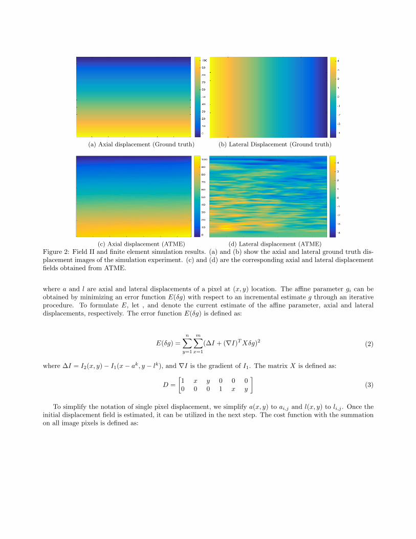
Figure 2: Field II and finite element simulation results. (a) and (b) show the axial and lateral ground truth dis-placement images of the simulation experiment. (c) and (d) are the corresponding axial and lateral displacementfields obtained from ATME.

where a and l are axial and lateral displacements of a pixel at (x, y) location. The affine parameter gi can beobtained by minimizing an error function E(δg) with respect to an incremental estimate g through an iterativeprocedure. To formulate E, let , and denote the current estimate of the affine parameter, axial and lateraldisplacements, respectively. The error function E(δg) is defined as:

E(δg) =

n∑y=1

m∑x=1

(∆I + (∇I)TXδg)2 (2)

where ∆I = I2(x, y)− I1(x− ak, y − lk), and ∇I is the gradient of I1. The matrix X is defined as:

D =

[1 x y 0 0 00 0 0 1 x y

](3)

To simplify the notation of single pixel displacement, we simplify a(x, y) to ai,j and l(x, y) to li,j . Once theinitial displacement field is estimated, it can be utilized in the next step. The cost function with the summationon all image pixels is defined as:

C(∆a1,1, · · · ,∆am,n,∆l1,1, · · · ,∆lm,n) =n∑

j=1

m∑i=1

{[I1(i, j)− I2(i+ ai,j , j + li,j)−∆ai,jI′2,a −∆li,jI

′2,l]

2

+ α1(ai,j + ∆ai,j − ai−1,j −∆ai−1,j)2 + β1(li,j + ∆li,j − li−1,j −∆li−1,j)

2

+ α2(ai,j + ∆ai,j − ai,j−1 −∆ai,j−1)2 + β2(li,j + ∆li,j − li,j−1 −∆li,j−1)2}.

(4)

where α and β are regularization terms for axial and lateral displacements respectively. By minimizing the costfunction using the initial guess (ai,j , li,j), the sub-sample axial and lateral displacements (∆ai,j ,∆li,j) for the totalimage are calculated. The initial displacements (ai,j , li,j) provided through the previous step are added to thesubsample displacements. This presents us the final lateral and axial displacements i.e. (ai,j +∆ai,j , li,j +∆li,j).Once the displacement field is estimated, its spatial gradient is calculated to obtain the strain image.

3. RESULTS

We tested our proposed method on acquired data from simulation and clinical trials. In this section, we alsopresent results of clinical trials using a previous work, DPAM,9 to compare with ATME. Estimation of lateraldisplacement is significantly more difficult mainly due to the poor resolution of ultrasound images in this direction,thereby limiting previous work to only calculate axial strain images. Simultaneous estimation of the displacementfiled for the entire image, however, allows us to substantially improve the quality of both axial and lateraldisplacements.

3.1 Simulation Experiments

Field II software11 is used to simulate ultrasound images. The phantom is homogenous and isotropic with aPoisson ratio of ν = 0.49. A uniform axial force profile is applied to the top of the phantom to generate 6% axialstrain. More than 12 scatterers are randomly distributed in each cubic millimeter of the phantom to generatefully developed speckles. Further details of the data acquisition are available in Ref. 9. The Axial and lateralground truth displacements and also the ones obtained by ATME are shown in Fig. 2. Note that the tissue ishomogenous, and therefore, the deformation is assumed to be planar.

Table 1: The SNR and CNR of the strain images of Fig. 5. Maximum values are in bold font.

Experiment SNR(DPAM) SNR(ATME) CNR(DPAM) CNR(ATME)

Patellar tendon flexion (distal portion) 4.77 10.06 5.46 11.98

Patellar tendon flexion (proximal portion) 6.41 9.17 3.51 3.24

MCL pure valgus 0.7 4.17 1.26 2.16

MCL pure valgus 3.20 6.59 6.28 10.70

Average 3.77 7.50 4.13 7.02

3.2 in-vivo Experiments

Ethics approval was obtained at both McGill University Health Centre (MUHC) and Concordia University tocollect ultrasound images of human subjects. Valgus stress was applied to the knee, and ultrasound data ofthe MCL was collected during the stress. In the second set of experiments, the subject freely flexed their knee,and ultrasound data was collected from the patellar tendon. Valgus stress and knee flexion generates strain inthe MCL and patellar tendon respectively, and we examined whether this strain can be measured using ATME.RF data was collected with an Alpinion ultrasound machine (Bothell, WA) with an L3-12 linear transducer atthe centre frequency of 11MHz and sampling frequency of 40MHz. Ligaments and tendons play a significant

(a) Axial Displacement (b) Lateral Displacement

(c) B-mode (d) Axial Strain

(e) Strain directions

Figure 3: Distal tendon motion during force flexion experiment. (a) and (b) show axial and lateral displacements.(c) is the B-mode image and red arrows represent the strain directions in the tendon. (d) and (e) depict theaxial strain and magnified strain directions respectively.

(a) Axial Displacement (b) Lateral Displacement

(c) B-mode (d) Axial Strain

(e) Strain directions

Figure 4: MCL during pure valgus stress experiment. (a) and (b) show axial and lateral displacements. (c) isthe B-mode image and red arrows represent the strain directions in the MCL. (d) and (e) depict the axial strainand magnified strain directions respectively.

role in musculoskeletal (MSK) biomechanics, and constantly change due to factors such as aging, injury, diseaseor exercise. Conventional B-mode ultrasonography has been widely used as a first line diagnostic modality forsuperficial structures such as the patellar tendon and MCL. Strain imaging captures dynamics of tissue motionand captures deformations of the patellar tendon and MCL, which are not directly available in B-mode images.These deformation patterns reveal mechanical properties of tendon and therefore may reveal important pathologyotherwise hidden in the B-mode scans.12

Fig. 3(a) and (b) show the displacement of the distal tendon (lower portion of patellar tendon connectedto tibia) during in-vivo forced flexion. The B-mode image is demonstrated in (c). Red arrows represent straindirections and their relative amplitudes in a region of interest. The patellar tendon is marked with blue arrows.The axial strain is shown in (d) wherein we can clearly distinguish the boundaries of tendon from rest of the

tissue. The strain arrows in (c) are magnified and depicted in (e) for better visualization. The results in (e) arein good agreement with our expectation of strain in the patellar tendon: the strain is relatively high close to thepatella (the hyperechoic dome-shaped structure in bottom left of (c) with the shadow underneath), where it isgetting pulled by the joint. The strain is also tensile (arrows pointing to the left) at the top, and compressive atthe bottom (arrows pointing to the right) in (e), as we expect from a bent structure (i.e. the patellar tendon).

Fig. 4(a) and (b) demonstrate the motion fields of MCL when the pure valgus stress is applied on the knee.(c) and (d) show the B-mode and strain images respectively. MCL is marked with blue arrows in (c). Straindirections which are shown with red arrows in (c) are enlarged in (e). Again, the strain field corresponds wellwith what we expect: high tension at the top where the extension is maximum in the bent MCL.

Fig. 5 shows B-mode images and also the strain fields calculated for the Patellar tendon and MCL duringflexion. For the purposes of comparison, strain images were also calculated using a previous work, DPAM.9 Inthe first row, the distal portion of the knee is shown while the forced flexion is applied to patellar tendon. Inthe second row, the same experiment is practiced but the proximal portion of the knee is depicted here. Thirdand forth rows show the MCL when pure valgus stress is placed on the knee. The valgus stress test is performedwith the knee at 30◦ of flexion.

The unitless metrics signal to noise ratio (SNR) and contrast to noise ratio (CNR) are used to quantitativelycompare the results:1

CNR =C

N=

√2(s̄b − s̄t)2σ2b + σ2

t

, SNR =s̄

σ(5)

where s̄t and s̄b are the spatial strain average of the target and background, and σ2t and σ2

b are the spatial strainvariance of the target and background, and s̄ and σ are the spatial average and variance of a window in thestrain image respectively. The corresponding SNR and CNR values are measured for both DPAM and ATMEmethods. CNR values are calculated between the target (tendon) and background (outside the target) windowseach of size 50 samples × 50 samples, and are provided in Tab. 1. SNR values are also shown in the table,which are calculated for the background windows. ATME provides substantially higher SNR and CNR valuescompared to DPAM.

4. CONCLUSION

In this paper, we introduce a novel technique to calculate both axial and lateral displacement fields between twoframes of RF data based on affine transformation prior. Optimization of the main global cost function involvessolving a sparse linear system which can be solved in real time and provide the displacement field of the entireimage simultaneously. We further applied strain imaging to patellar tendon and MCL, and showed that our pro-posed technique can be used to predict displacement and strain fields in these tissues. Future work will utilizethese dynamical measurements of the patellar tendon and MCL to both improve diagnosis and manage treatment.

Acknowledgement

This work was supported by Richard and Edith Strauss Canada Foundation.

REFERENCES

[1] Ophir, J., Alam, S., Garra, B., Kallel, F., Konofagou, E., Krouskop, T., and Varghese, T., “Elastography:ultrasonic estimation and imaging of the elastic properties of tissues,” Proceedings of the Institution ofMechanical Engineers, Part H: Journal of Engineering in Medicine 213(3), 203–233 (1999).

[2] Parker, K. J., Doyley, M., and Rubens, D., “Imaging the elastic properties of tissue: the 20 year perspective,”Physics in medicine and biology 56(1), R1 (2010).

[3] Gennisson, J.-L., Deffieux, T., Fink, M., and Tanter, M., “Ultrasound elastography: principles and tech-niques,” Diagnostic and interventional imaging 94(5), 487–495 (2013).

(a) B-mode (b) DPAM strain (axial) (c) ATME strain (axial)

(d) B-mode (e) DPAM strain (axial) (f) ATME strain (axial)

(g) B-mode (h) DPAM strain (axial) (i) ATME strain (axial)

(j) B-mode (k) DPAM strain (axial) (l) ATME strain (axial)

Figure 5: comparison between ATME and DPAM methods. (a), (b), and (c) show distal area of patellar tendonduring force flexion experiment. (d), (e), and (f) are proximal region of patellar tendon. (g)-(l) are B-mode andstrain images of MCL during pure valgus stress experiment.

[4] Zahiri-Azar, R. and Salcudean, S. E., “Motion estimation in ultrasound images using time domain crosscorrelation with prior estimates,” IEEE Transactions on Biomedical Engineering 53(10), 1990–2000 (2006).

[5] Treece, G., Lindop, J., Chen, L., Housden, J., Prager, R., and Gee, A., “Real-time quasi-static ultrasoundelastography,” Interface focus , rsfs20110011 (2011).

[6] Rivaz, H., Boctor, E., Foroughi, P., Zellars, R., Fichtinger, G., and Hager, G., “Ultrasound elastography: adynamic programming approach,” IEEE transactions on medical imaging 27(10), 1373–1377 (2008).

[7] J Hall, T., E Barboneg, P., A Oberai, A., Jiang, J., Dord, J.-F., Goenezen, S., and G Fisher, T., “Recentresults in nonlinear strain and modulus imaging,” Current medical imaging reviews 7(4), 313–327 (2011).

[8] Shams, R., Boily, M., Martineau, P. A., and Rivaz, H., “Dynamic programming on a tree for ultrasoundelastography,” in [SPIE Medical Imaging ], 97901F–97901F, International Society for Optics and Photonics(2016).

[9] Rivaz, H., Boctor, E. M., Choti, M. A., and Hager, G. D., “Real-time regularized ultrasound elastography,”IEEE transactions on medical imaging 30(4), 928–945 (2011).

[10] Bergen, J. R., Anandan, P., Hanna, K. J., and Hingorani, R., “Hierarchical model-based motion estimation,”in [European conference on computer vision ], 237–252, Springer (1992).

[11] Jensen, J. A., “Field: A program for simulating ultrasound systems,” in [10th Nordicbaltic conference onbiomedical imaging, vol. 4, supplement 1, part 1: 351–353 ], Citeseer (1996).

[12] Chimenti, R. L., Flemister, A. S., Ketz, J., Bucklin, M., Buckley, M. R., and Richards, M. S., “Ultrasoundstrain mapping of achilles tendon compressive strain patterns during dorsiflexion,” Journal of biomechan-ics 49(1), 39–44 (2016).