iii 

 

Acknowledgements 

"For by him all things were created: things in heaven and on earth, visible and invisible, 

whether thrones or powers or rulers or authorities; all things were created by him and for him." 

                  Colossians 1:16 

First and foremost I would like to thank my parents.  Dad, without your encouragement to see 

beyond my trials I would have given up long ago.  I consider it an honor to have you as a father, 

a mentor and a friend.  Mom, thank you your unwavering love, regardless of my 

accomplishments or failures.  I am proud to be your son and thankful for every smile and hug 

that awaits me every time I see you.   

Dr. Pollock, I have learned as much from watching you as I have from listening to your 

feedback.  Your care for your students above your self is evident, and an inspiration.  To all 

those that helped keep me sane throughout this process and remind me that there is more to 

life than a dissertation:  Alan, Neil, Mike, Chuck, Jacob, Rebekah, Jessie, Laura, and Kristina your 

friendship means more than you know. 

Also, this dissertation would not have been possible without funding for this project, which was 

provided by the U.S. Department of Transportation (USDOT), Transportation Northwest 

(TransNow) Regional Research Center through contract number 430820.  The commercial all‐

thread tieback rods were provided by Williams Form Engineering Corporation.   

 

iv 

 

ULTRASONIC DETECTION OF SIMULATED CORROSION IN 1 INCH DIAMETER STEEL TIEBACK RODS 

Abstract 

By Karl R. Olsen Washington State University 

August 2009  

Chair:  David G. Pollock 

 

The research presented investigates the use of pulse‐echo ultrasonic techniques to identify 

simulated corrosion in steel rods.   The primary objective was to quantify loss of cross section 

due to corrosion of steel tieback rods in earth retention systems.   Current techniques require 

excavation of rods for inspection; however this proposed nondestructive method utilizes the 

end of the rod protruding from the embankment in conjunction with an ultrasonic pulse‐echo 

system to estimate the reduction in load capacity of the rod.  An ultrasonic wave was initiated 

with a piezoelectric transducer coupled to the end of the rod.  The same transducer converted 

the returning wave into an ultrasonic signal which was used to determine the physical 

geometry of simulated corrosion.   The ultrasonic signal could identify the location of simulated 

corrosion on the rod using the time between the main bang and the first flaw echo.   The 

diameter of simulated corrosion could be determined from the time between the back echo 

and the first trailing echo.  The length of the corroded region was correlated with the ratio of 

the first trailing echo and the back echo.   Flaw echoes from simulated corrosion could be 

detected for all transition angles down to 5o.  A decrease in the transition angle resulted in a 

time delay in the arrival of the flaw echo up to 23.8 µs for the 5° transition, which corresponds 

 

v 

 

to 5.5 in. in steel rods.   Williams all‐thread commercial tieback rods were tested.   Ultrasonic 

signals generated in Williams rods embedded in various soils showed negligible attenuation of 

signal amplitude.  Simulated corrosion geometry, including location, diameter, and length were 

inspectable in 1.0 in. diameter Williams tieback rods.  Testing showed that ultrasonic testing 

could be used detected in rod lengths up to 40 feet.   

   

 

vi 

 

Contents 

1  Introduction and Objectives .................................................................................................... 1 

1.1  Tieback Rods ..................................................................................................................... 1 

1.2  Problem Statement .......................................................................................................... 2 

1.3  Research Objectives ......................................................................................................... 3 

1.3.1  Detect Physical Geometry of Simulated Corrosion in Steel Rods ............................. 3 

1.3.2  Evaluate Threaded Williams Tieback Rods ............................................................... 4 

1.4  Outline of Dissertation Contents ..................................................................................... 4 

2  Background and Literature Review ......................................................................................... 6 

2.1  Pressure Wave Properties ................................................................................................ 6 

2.2  Two methods for Solving the Wave Equation .................................................................. 8 

2.3  Background in Ultrasonic Waves in Rods ....................................................................... 13 

2.3.1  Ultrasonic Wave ...................................................................................................... 14 

2.4  Ultrasonic Applications .................................................................................................. 17 

2.4.1  Previous Ultrasonic Research ................................................................................. 17 

3  Experimental Setup and Testing ............................................................................................ 22 

3.1  Experimental Setup ........................................................................................................ 22 

3.2  Labview Program ............................................................................................................ 23 

3.3  Transducer Characterization and Selection ................................................................... 23 

3.4  Wavelength in Steel Rod ................................................................................................ 26 

3.5  End Preparation and Transducer Coupling .................................................................... 27 

3.6  Steel Rods Used in Testing ............................................................................................. 28 

3.7  Velocity Calculation for Steel Rods ................................................................................ 29 

4  Detecting Physical Geometry of Simulated Corrosion .......................................................... 33 

4.1  Location of Leading Edge of Simulated Corrosion ......................................................... 33 

4.2  Diameter Characterization ............................................................................................. 36 

4.3  Length of Simulated Corrosion Characterization ........................................................... 45 

4.3.1  Change in Frequency Content of Back Echo for Length of Simulated Corrosion ... 46 

 

vii 

 

4.3.2  Change in Back Echo Amplitude with Length of Simulated Corrosion ................... 53 

4.4  Transition Characterization ............................................................................................ 57 

4.4.1  Linear Transitions with Notches ............................................................................. 62 

5  Williams Commercial Tieback Rod Testing ............................................................................ 69 

5.1  Types of Tieback Rods Used in Geotechnical Applications ............................................ 69 

5.2  Projected Length of Rod to be Inspected ....................................................................... 72 

5.3  Signal Attenuation for Williams Rods in Soil .................................................................. 74 

5.3.1  Soil Characterization ............................................................................................... 75 

5.3.2  Soil Preparation ....................................................................................................... 77 

5.3.3  Signal Attenuation for Tieback Rods in Soil ............................................................ 78 

5.4  Actual Tieback Rods with Flaws ..................................................................................... 83 

5.4.1  Location of Simulated Corrosion ............................................................................ 83 

5.4.2  Diameter of Simulated Corrosion ........................................................................... 85 

5.4.3  Length of Simulated Corrosion ............................................................................... 87 

5.4.4  Transition of Simulated Corrosion .......................................................................... 89 

6  Inspection Procedures ........................................................................................................... 93 

6.1  Inspection of Simulated Corrosion ................................................................................. 93 

6.2  End preparation and Transducer Coupling .................................................................... 97 

6.3  Commercial Tieback Rod Testing ................................................................................... 98 

6.3.1  New Construction ................................................................................................... 99 

6.3.2  Existing Construction ............................................................................................ 102 

7  Summary and Conclusions .................................................................................................. 106 

 

   

 

viii 

 

List of Figures  

Figure 1.  Sheet pile earth retention walls (US Army Corps of Engineers, 1994) ........................... 1 

Figure 2.  Mathematical wave characterization ............................................................................. 6 

Figure 3.  Diagram of Snell's Law .................................................................................................... 7 

Figure 4.  Dispersion diagram for a 0.79 in. diameter steel rod in a vacuum (Beard, Lowe, & Cawley, 2001) ................................................................................................................................ 11 

Figure 5.  Ray approach for solution of wave equation ................................................................ 13 

Figure 6.  Standard ultrasonic signal from 1.0 ft. long 1.0 in. diameter circular rod ................... 14 

Figure 7.  Ultrasonic Signal for 3.0 ft. long 1.0 in. diameter rod with a 2.0 in. length of  0.5 in. reduced diameter starting at 17.0 in. from the transducer ......................................................... 15 

Figure 8.  Spacing of trailing echoes for 3.0 ft. long 1.0 in. diameter rod with a 2.0 in. length of  0.5 in. diameter simulated corrosion............................................................................................ 15 

Figure 9.  Trailing echoes reflection diagram ............................................................................... 16 

Figure 10. End angle effect on signal strength (Beard, Lowe, & Cawley, 2001) ........................... 19 

Figure 12.  Shift in signal centroid due to angular deformation of rod (Pollock, 1997) ............... 20 

Figure 11.  Deformation of the rod (Pollock, 1997) ...................................................................... 20 

Figure 13.  Time traces for a 1.2 m straight rod and a similar rod with constant curvature corresponding to 30mm of center deflection.  (Beard, Lowe, & Cawley, 2001) .......................... 21 

Figure 14.  Ultrasonic pulse‐echo test setup ................................................................................ 22 

Figure 15.  Transducer amplitude comparison on a rod with no simulated corrosion ................ 24 

Figure 16.  Flaw echo and back echo of rod with a 0.25 in. reduction in diameter ..................... 26 

Figure 17.  Minimum detectable flaw dimension in steel for multiple ultrasonic pulse frequencies ................................................................................................................................... 27 

Figure 18.  Williams commercial tieback rod and 12L14 rod stock used in testing ..................... 28 

Figure 19. Full ultrasonic signal for 1.0 ft. long 1.0 in. diameter 12L14 steel rod for calculating wave speed ................................................................................................................................... 30 

Figure 20.  Main bang and first and second back echoes for 1.0 ft. long 1.0 in. diameter steel rod....................................................................................................................................................... 31 

Figure 21.   Actual corrosion of a steel rod ................................................................................... 33 

 

ix 

 

Figure 22.   Simulated corrosion of a steel rod ............................................................................. 33 

Figure 23.  3 ft. long 1.0 in. diameter rods with 2.0 in. length of 0.5 in. diameter simulated corrosion used for detection of simulated corrosion location ..................................................... 34 

Figure 24. Ultrasonic signals for simulated corrosion located at 8.94 in., 16.06 in., and 23.03 in. from the end of the rod. ............................................................................................................... 35 

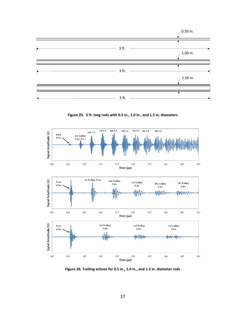
Figure 25.  3 ft. long rods with 0.5 in., 1.0 in., and 1.5 in. diameters ........................................... 37 

Figure 26. Trailing echoes for 0.5 in., 1.0 in., and 1.5 in. diameter rods ...................................... 37 

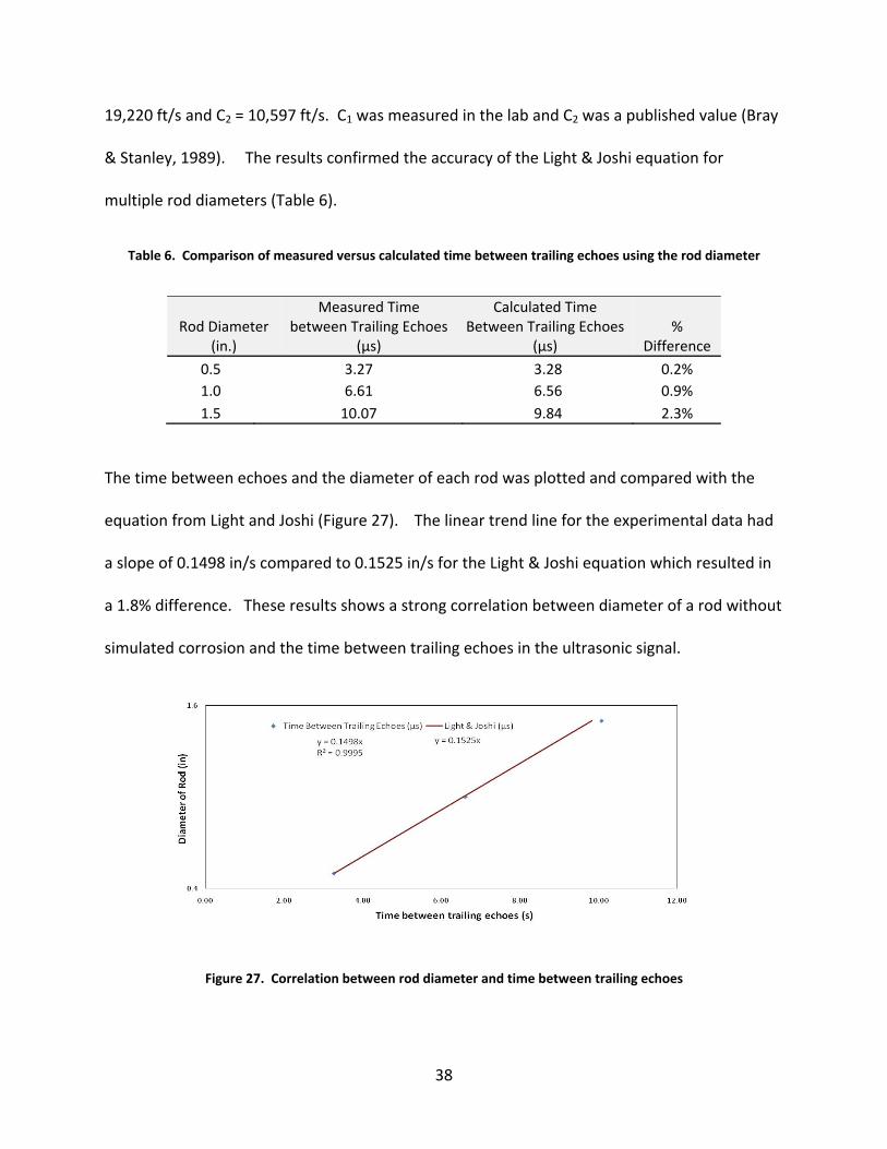
Figure 27.  Correlation between rod diameter and time between trailing echoes ..................... 38 

Figure 28.  1.0 in. diameter rod with  0.5 in. simulated corrosion diameter compared with 0.5 in. diameter  and 1.0 in. diameter rods ............................................................................................. 39 

Figure 29.  Comparison of ultrasonic signals for 1.0 in. diameter  rod with 0.5 in. diameter simulated corrosion versus 0.5 in. and 1 in. diameter rods ......................................................... 40 

Figure 30.  3 ft. long 1.0 in. diameter rods with 2.0 in. length of 0.25 in., 0.50 in., or 0.75 in. diameter simulated corrosion ...................................................................................................... 42 

Figure 31. Ultrasonic signals for simulated corrosion diameters 0.50 in., and 0.75 in. ............... 43 

Figure 32.  Percent reduction of original load capacity for simulated corrosion in a 1 in. diameter rod ................................................................................................................................................. 44 

Figure 33.  Signal waveform and frequency content for 5 MHz M1041 Olympus NDT transducer....................................................................................................................................................... 46 

Figure 34.  Back echo of 1.0 ft. long rod with a 0.5 in. simulated corrosion diameter with and without zeros ................................................................................................................................ 47 

Figure 35.  FFT for 3.0 ft. long rods with 0.5 in., 1.0 in., and 1.5 in. diameters ............................ 48 

Figure 36.  FFT for back echo of 1.0 in. diameter rods with 1.0 ft., 3.0 ft., and 10.0 ft. lengths .. 48 

Figure 37.  1.0 in. diameter 1.0 ft. long rods with different lengths of simulated corrosion ....... 49 

Figure 38.  Frequency analysis of first back echo for multiple lengths of simulated corrosion in a 1.0 in. diameter 1.0 ft. long steel rod ........................................................................................... 50 

Figure 39.  3.0 ft. long 1.0 in. diameter rods with 2.0 in., 6.0 in., and 8.0 in. lengths of simulated corrosion starting at 9 in. along the rod ....................................................................................... 51 

Figure 40.  Peak frequency of the back echo for 3.0 ft. long rods with 2.0 in., 6.0 in., and 10.0 in. lengths of simulated corrosion. .................................................................................................... 52 

Figure 41.  Back echo and first trailing echo for 1.0  ft. long rods with multiple lengths of simulated corrosion ...................................................................................................................... 54 

 

x 

 

Figure 42.  Ratio of trailing echo peak amplitude and back echo peak amplitude for 1.0 in. rods....................................................................................................................................................... 55 

Figure 43.  Comparison of reflection from the simulated corrosion surface ............................... 56 

Figure 44.  Ratio of trailing echo and back echo for 2.0 in., 6.0 in. and 10.0 in. long simulated corrosion in 3.0 ft. long 12L14 rods .............................................................................................. 57 

Figure 45.  1.0 ft. long 1.0 in. diameter rods with multiple  transition angles used for detection of simulated corrosion .................................................................................................................. 58 

Figure 46.  Ultrasonic signal for 90°, 45°, 30°, 15°, 10° and 5°  transition angles ......................... 59 

Figure 47.  Delay in detectable flaw echo versus transition angle ............................................... 60 

Figure 48.  6.0 in. long 1.0 in. diameter rods with 0.125 in. deep 0.25 in. wide notches  located 0.5 in., 1.0 in., and 2.0 in. from the end of the rod ...................................................................... 61 

Figure 49.  Notch echo comparison for notches located 0.5 in., 1.0 in., and 2.0 in. from the end of the rod ...................................................................................................................................... 62 

Figure 50.  1.0 ft. long 1.0 in. diameter rods with multiple transition angles .............................. 63 

Figure 51.  Normalized maximum amplitude of flaw echo versus transition angle ..................... 64 

Figure 52.  Longitudinal wave reflection from transition surface ................................................ 65 

Figure 53.  Shear wave reflection from transition surface ........................................................... 67 

Figure 54.  Upset thread and all‐thread rods ............................................................................... 69 

Figure 55.  Comparison of 10 ft. long Williams threaded rod and 12L14 smooth steel rod ........ 70 

Figure 56.  Trailing echo comparison for 12L14 smooth rod and Williams threaded rod ........... 71 

Figure 57.  Rectified time domain signals for 1 ft., 3 ft. and 6 ft. long Williams rods .................. 72 

Figure 58.  Signal attenuation for 1.0 ft., 3.0 ft., and 6.0 ft. long Williams rods. ......................... 73 

Figure 59.  Boxes constructed for signal attenuation tests in soils .............................................. 75 

Figure 60.  Grain size distribution for sand and soil samples ....................................................... 76 

Figure 61.  Atterberg limit test of Palouse soil ............................................................................. 77 

Figure 62.  Exponential decay of back echo peaks in 3.0 ft. long Williams rod ............................ 79 

Figure 63.  Transmittance for steel with water and concrete surrounding media ...................... 82 

Figure 64.  3.0 ft. long 1.0 in. diameter Williams tieback rods with 2.0 in. length of 0.5 in. simulated corrosion diameter at 9.28 in., 15.97 in., and 22.84 in. along the rod ........................ 83 

 

xi 

 

Figure 65. Ultrasonic signals from 3.0 ft. long 1.0 in. diameter Williams tieback rods with 2.0 in. length of 0.5 in. diameter simulated corrosion at 9.28 in., 15.97 in., and 22.84 in. along the rod........................................................................................................................................................ 84 

Figure 66.  3.0 ft. long 1.0 in. diameter Williams rods with 2.0 in. lengths of 0.5 in. and 0.75 in. diameter simulated corrosion ...................................................................................................... 85 

Figure 67.  Comparison of Williams rods with 0.5 in. and 0.75in. diameter of simulated corrosion....................................................................................................................................................... 86 

Figure 68.  3.0 ft. long 1.0 in. diameter Williams tieback rods with 2.0 in. and 10.0 in. lengths of 0.5 in. diameter simulated corrosion............................................................................................ 87 

Figure 69.  Frequency of ultrasonic signal of Williams rods with 2.0 in and 8.0 in. lengths of simulated corrosion. ..................................................................................................................... 88 

Figure 70.  Ratio of trailing echo and back echo for 2.0 in. and 10.0 in. long simulated corrosion in 3.0 ft. long Williams rods .......................................................................................................... 88 

Figure 72.  Full ultrasonic signal for 2 in. length of 0.5 in. diameter simulated corrosion with 45° transition angle for Williams tieback rod ..................................................................................... 89 

Figure 71.  Rod used for simulated corrosion detection with a 45° transition angle ................... 89 

Figure 73.  First back echo and successive trailing echoes for 2 in. simulated corrosion with 45° transition ....................................................................................................................................... 90 

Figure 74. Frequency of back echo of 2 in. long 0.5 in. diameter simulated corrosion with 45° transition in Williams rod .............................................................................................................. 91 

Figure 75.  Ratio of trailing echo and back echo for 2.0 in. simulated corrosion length with 45° transition in 3.0 ft. long  Williams rods ......................................................................................... 92 

Figure 76 Ultrasonic pulse‐echo signal for 12L14 smooth steel rod and Williams steel all‐thread tieback rod both with simulated corrosion .................................................................................. 93 

Figure 77.  Location of the leading edge for the main bang and flaw echo ................................. 94 

Figure 78.  First back echo and subsequent trailing echoes for inspection of simulated corrosion diameter inspection in 1.0 in. diameter 12L14 steel rod and 1.0 in. diameter Williams rod ...... 95 

Figure 79.  Minimum detectable flaw dimension in steel ............................................................ 97 

 

   

 

xii 

 

List of Tables 

Table 1.  Commercial transducers used in selection process ....................................................... 25 

Table 2. Properties for 12L14 steel and Williams grade 75 tieback rod ....................................... 29 

Table 3. Arrival time of ultrasonic signal components. ................................................................ 32 

Table 4.  Wave speed of 12L14 steel and 75 ksi Williams steel rods ............................................ 32 

Table 5.  Comparison of measured and calculated simulated corrosion locations ...................... 36 

Table 6.  Comparison of measured versus calculated time between trailing echoes using the rod diameter ........................................................................................................................................ 38 

Table 7.  Calculated diameter for 1.0 in. diameter rod with 0.5 in. diameter simulated corrosion, 0.5 in. diameter rod, and 1.0 in. diameter rod. ............................................................................ 41 

Table 8.  Calculated diameter for 1.0 in. diameter rod with 0.5 in. and 0.75 in. diameter simulated corrosion ...................................................................................................................... 44 

Table 9.  Maximum amplitudes of back echo and first trailing echo ........................................... 55 

Table 10.  Angle of longitudinal wave reflection from transition surface .................................... 66 

Table 11.  Angle of shear wave reflection from transition surface .............................................. 68 

Table 12.  Soil characterization ..................................................................................................... 76 

Table 13.  Results of Atterberg limit test for Palouse soil ............................................................ 77 

Table 14.  Water content for each soil test .................................................................................. 78 

Table 15.  Attenuation coefficients of the ultrasonic signal for Williams tieback rods in soils .... 80 

Table 16.  Normalized attenuation coefficients of the ultrasonic signal for Williams tieback rods in soils............................................................................................................................................ 81 

Table 17.  Comparison of measured and calculated location of simulated corrosion ................. 85 

Table 18.  Time between trailing echoes for 0.5 in. and 0.75 in. simulated corrosion diameter  86 

Table 19.  Calculated simulated corrosion location for Williams rod with 45° transition angle .. 90 

Table 20.  Comparison of measured and calculated diameter of simulated corrosion for Williams rod with 45° transition angle ........................................................................................................ 91    

 

1 

 

1 Introduction and Objectives 

In 2002, just east of downtown Cleveland, Ohio, several tieback rods in a sheet pile earth 

retaining wall failed (Esser & Dingeldein, 2007).   The failure was due to corrosion and caused a 

near collapse of the wall.  Corrosion in structural steel tieback rods causes a decrease in cross‐

sectional area, limiting tensile load capacity.  Tieback rods are typically buried in soil, 

eliminating the option of visual inspection without excavation.   The research in this study 

evaluated ultrasonic testing as a method of detecting simulated corrosion in steel rods.  

1.1 Tieback Rods 

Tieback rods are a vital component of sheet pile retaining walls.   The rods connect  the outer 

support structure to anchors (or “deadman”) buried in the soil (Figure 1.)   The first tieback rods 

 

Figure 1.  Sheet pile earth retention walls (US Army Corps of Engineers, 1994) 

Wale

Sheet Piling 

Wale Tie Rod

Tie RodConcrete Deadman 

Sheet Piling Anchor 

Sheet Piling 

a. Tie rods and dead man 

b. Tie rods and anchor wall 

 

2 

 

used in commercial construction consisted of A36 (36 ksi yield strength) round stock with upset 

threads at each end.  The majority of rods used in current construction practices, including the 

Williams Form Corporation tieback rods used in this research, are an all‐thread rod with a yield 

stress of 75 ksi.    Developments in corrosion technology have introduced several improvements 

to tieback rods.   Numerous methods for corrosion resistance have been developed (Williams 

Form Engineering Corp, 2008):  

• Epoxy coating • Pre-grouted rods • Hot dip galvanizing • Extruded polyethylene coating • Coal tar epoxy • Corrosion inhibiting wax or sheath with grease • Heat shrink tubing

The selection of rods and corrosion resistance techniques is typically determined by a 

geotechnical engineer depending upon site conditions (US Army Corps of Engineers, 1994).  

1.2 Problem Statement  

Older tieback rods are susceptible to corrosion, which may compromise the structural integrity 

of confined earth embankment systems supporting transportation structures and facilities.  

Corrosion in buried metal tieback rods is difficult to detect, and the magnitude of associated 

cross‐section loss is particularly difficult to quantify.  Since the exposed heads of tieback rods 

(at the sheet piling face) are typically accessible, an ultrasonic pulse‐echo inspection technique 

has potential for detecting and quantifying cross‐section loss due to corrosion.  Previous 

ultrasonic pulse‐echo research of steel rods has investigated several geometric properties.  This 

 

3 

 

ultrasonic characterization must be expanded to address a more comprehensive 

characterization of the rod to accurately assess the reduction in load capacity of a commercial 

tieback rods. 

1.3 Research Objectives  

The objectives for this research were divided into two categories.  First, use ultrasonic 

inspection to assess the physical geometry of simulated corrosion in steel rods.   Second, 

evaluate Williams all‐thread tieback rods.   

1.3.1 Detect Physical Geometry of Simulated Corrosion in Steel Rods 

The first set of objectives involved the use of ultrasonic signals to detect the critical physical 

geometries of a steel rod with simulated corrosion.  In previous research, several physical 

geometries have been detected, including location of flaws, curvature of the rod, diameter of 

the flaw, and the effect of angled cuts at the end of the rod.  The following research objectives 

were investigated to confirm previous research and develop new techniques to detect other 

physical geometries.  

1. Detect the location of simulated corrosion. 2. Detect the diameter of simulated corrosion. 3. Detect the length of simulated corrosion. 4. Investigate the effect of simulated corrosion transitions on the flaw echo in ultrasonic 

signals. 5. Develop a normalized amplitude method for assessing attenuation in the transition of 

simulated corrosion. 

 

4 

 

1.3.2 Evaluate Threaded Williams Tieback Rods 

The second set of objectives involved evaluating Williams tieback rods.   The all‐thread surface 

and the surrounding soil affect the ultrasonic wave as it travels through the rod.   The following 

research objectives were investigated to characterize the ultrasonic signal in Williams tieback 

rods. 

1. Determine if ultrasonic response signal can be identified in commercial threaded tieback rods. 2. Determine the effect of various soils on attenuation of ultrasonic signals in commercial threaded 

tieback rods. 3. Identify simulated corrosion in threaded tieback rods. 

1.4 Outline of Dissertation Contents 

This dissertation consists of seven chapters.  Some background regarding ultrasonic waves is 

provided in the second chapter.   Starting with the fundamentals of wave propagation, the 

theory is developed and presented, with applications to nondestructive testing.   Previous 

research regarding ultrasonic waves in rods is also summarized in Chapter two.  The third 

chapter describes the experimental setup used in the research presented in the dissertation.  

Transducer coupling and basic wave velocity tests are included in Chapter three.   Chapter four 

examines the physical geometries of simulated corrosion detectable with ultrasonic pulse echo 

methods.  This includes location, length, diameter, and transition characterization.  Chapter five 

investigates the use of ultrasonic waves in threaded Williams tieback rods.   Signal attenuation 

in soils, maximum detectable rod length, and simulated corrosion in Williams rods are 

 

5 

 

evaluated.   Chapter six addresses guidelines for developing an ultrasonic inspection strategy 

for use by a state Department of Transportation (DOT).  Finally, conclusions are presented in 

the seventh chapter. 

   

 

6 

 

2 Background and Literature Review 

This chapter presents a background of ultrasonic waves.  An overview of fundamental wave 

propagation provides the basis for understanding ultrasonic waves.   The use of ultrasonic 

waves in nondestructive testing (NDT) is presented, including previous research pertaining 

specifically to steel rods. 

2.1 Pressure Wave Properties 

A wave is a disturbance that propagates through time and space.  Energy is transferred from 

one point to another via waves.  A single frequency bulk wave is characterized mathematically 

by the wavelength (λ) and amplitude (A) of the signal (Figure 2).  The wavelength is the distance 

between two adjacent peaks in the wave cycle and the amplitude is the maximum displacement 

of the disturbance from the undisturbed position.  The frequency (f) of the wave is defined as  

 

 Figure 2.  Mathematical wave characterization 

 

 

7 

 

the number of oscillations that occur in one second and the period (T) is the time to complete 

one oscillation.   

Phase Velocity 

The speed at which the bulk wave travels though a medium is called the phase velocity (νp) and 

is calculated with the following equation (Main, 1988). 

             Equation 1 

The phase velocity is dependent upon the type of wave traveling in the medium.  Longitudinal 

and shear waves will be considered in this research.  Longitudinal waves exhibit particle motion 

in the direction of wave propagation.  Shear waves exhibit particle motion orthogonal to the 

direction of wave propagation.   

Snell's Law  

When a longitudinal wave encounters a boundary surface, longitudinal and shear waves are 

reflected back into the medium at angles determined by Snell's Law (Figure 3).  The resulting  

longitudinal wave reflects at an angle equal to the incident angle.  The reflected shear wave has 

θ1

θ2

θ1

 

Figure 3.  Diagram of Snell's Law 

 

8 

 

a reflected angle (θ2) that is dependent upon the incident angle (θ1), the incoming longitudinal 

wave speed (c1), and the reflected  shear wave speed (c2). 

Attenuation 

As a wave propagates through a medium, the wave displacement decreases with distance due 

to scattering and absorption.  Scattering is the reflection of the wave in directions other than its 

original direction of propagation.  Absorption is the conversion of the wave energy to other 

forms of energy.  Attenuation is the decay rate of the wave as it propagates through material 

due to scattering and absorption.  The attenuation of displacement in a wave as it travels 

through a medium is characterized by Equation 2,  where wo is the initial displacement,  α is the 

coefficient of attenuation, and x is the distance along the rod (Kolsky, 1963).   

 

   Equation 2 

 

2.2 Two methods for Solving the Wave Equation 

In a bounded medium, such as the steel rods used in this research, waves are reflected from 

the boundaries.  Solutions can be found by solving the wave equation with cylindrical 

boundaries.  The wave equation, in cylindrical coordinates, in an unbounded medium is defined 

as follows: 

 

 

9 

 

    ∆     Equation 3 

    ∆    Equation 4 

    ∆    Equation 5 

where z is the axis of the waveguide, ρ is the density of the medium, ur, uθ, uz, are the local 

displacements of the medium along each axis, r is the radius, t is time, ι and µ are Lame's 

constants. The dilatation (Δ) and elements of the rotation tensor (ωr, ωθ, ωz) are given by: 

∆            Equation 6 

               Equation 7 

                  Equation 8 

                   Equation 9 

The stress in the rod is used as a boundary condition.  At the surface of the rod, the three stress 

components (σrr,σrθ,σrz) must equal zero.  The stress‐deformation relations are as follows: 

     Equation 10 

      Equation 11 

    Equation 12 

 

10 

 

General solutions to the wave equations are considered for harmonic waves with exponential 

propagation in the z direction along a rod.  For the general case of vibration, the equations for 

displacements are as follows: 

 Equation 13 

 Equation 14 

 Equation 15 

For longitudinal waves the displacement is a function of z and r, therefore the derivative with 

respect to θ is zero.  The displacement uθ is also zero due to symmetry.  Therefore, Equation 3, 

Equation 4 and Equation 5 reduce to: 

∆     ∆ ∆     Equation 16 

         Equation 17 

where: 

   Equation 18 

   Equation 19 

Where the frequency of the waves is p/2π and the phase velocity is given by p/γ Since h' and κ' 

are constants, setting r' = h'r and r'' = κ'r converts Equation 16  and Equation 17 into zero order 

and first order forms of the Bessel equation, respectively.       

 

11 

 

∆     ∆ ∆     Equation 20 

         Equation 21 

 

At this point two separate methods are available for solving the wave equation.  These include 

the mode and the ray approach.  Each of the methods are described below. 

Mode Approach (Dispersion Diagrams) 

The solution to the wave equation using the Bessel function subject to appropriate boundary 

conditions results in a number of solutions that form continuous propagating modes of 

vibration.  The velocity‐frequency relationship of the individual modes can be displayed as a set 

dispersion curves (Figure 4).  Each line in the diagram represents a different mode of vibration.   

 

Figure 4.  Dispersion diagram for a 0.79 in. diameter steel rod in a vacuum (Beard, Lowe, & Cawley, 2001) 

 

12 

 

Flexural modes are noted by "F", longitudinal modes are noted by "L", and the torsional mode is 

noted by "T".  This facilitates determination of the frequency to generate in order to initiate 

specific modes.   The frequency of the ultrasonic signal generated in the following research is in 

the range that will initiate hundreds of modes of vibration.   

 

Ray Approach  

The second approach for solving the wave equation is the ray approach.  This method involves a 

simplification of Equation 20 using a differentiation by parts identity. 

∆ ∆    Equation 22 

Assume that Δ varies rapidly compared to changes in r'.  Then r' can be pulled outside the 

derivative.  The simplification is based on the assumption that the wavelength of the ultrasonic 

signal is significantly smaller than the diameter of the rod.   

∆ ∆    Equation 23 

The solution for this equation is given as: 

∆  Equation 24 

This solution approximates the wave as a bulk wave.  Also, since the wavelength is assumed to 

be significantly smaller than the diameter of the rod, the surface of the rod can be 

approximated as a flat plate.  Assuming a point source for the generation of the wave, Figure 5 

 

13 

 

  

 

represents four of the paths with the shortest travel distance the wave can take from the 

source to a common point at the end of the rod for longitudinal wave propagation.  This 

depiction allows insight into how the wave propagates through the rod. 

The research presented uses the ray approach as opposed to the mode approach for two 

reasons.  First, the pulse‐echo method generates a pulse in the steel rod rather than a 

continuous vibration.  Second, the diameter of the steel rods inspected (1.0 in.) is 

approximately 20 times greater than  wavelength generated by the 5MHz ultrasonic transducer 

in steel.  This allows for the assumption used in the ray approach. 

2.3 Background in Ultrasonic Waves in Rods 

Ultrasonic waves are defined as cyclic pressure waves with a frequency greater than the 

threshold of human hearing.  Although human hearing varies from person to person, the 

ultrasonic range is considered to include all pressure waves above 20 kHz.  The following 

section presents some fundamental concepts and terminology from previous literature.  This 

Source 

Figure 5.  Ray approach for solution of wave equation 

 

14 

 

will establish the theoretical foundation that will be built upon to compile a more complete 

understanding of ultrasonic waves in rods. 

2.3.1 Ultrasonic Wave  

Ultrasonic waves can be initiated in steel rods using a piezoelectric transducer.  An electric 

signal was sent to the transducer converting electrical energy to mechanical energy in the form 

of a pressure wave.  When coupled to the end of a steel rod the wave is generated in the steel 

rod and proceeds to travel the length of the rod.  At this point a receiving transducer can detect 

the signal at the other end of the rod, or if the end of the rod is not accessible, the wave 

reflects from the end surface of the rod and travels back to the transducer.  As the wave 

returns to the front end, the transducer converts the mechanical energy into electrical energy, 

and the electrical signal is recorded by the computer.  The ultrasonic signal for a straight rod 

without any flaws is shown below (Figure 6). The main bang represents the generation of the 

ultrasonic wave.  The small signal following the main bang is a ringing out of the piezoelectric 

transducer.   The next signal that appears is the first back echo, which represents the front of 

 Figure 6.  Standard ultrasonic signal from 1.0 ft. long 1.0 in. diameter circular rod 

 

15 

 

the pressure wave that reflected from the end of the rod and returned to the transducer.  

Several trailing echoes follow the first back echo, and these will be discussed later in more 

depth.   For a rod with a flaw, an early echo will appear in the signal dependent upon the 

location of the flaw along the rod.   A portion of the ultrasonic wave will reflect from the flaw 

and return to the transducer before the back echo (Figure 7).  Further inspection of the 

ultrasonic signal reveals a consistent spacing between the trailing echoes after the back echo 

(Figure 8).   Research has shown (Light & Joshi, 1987) that the spacing is due to mode  

 Figure 7.  Ultrasonic Signal for 3.0 ft. long 1.0 in. diameter rod with a 2.0 in. length of  0.5 in. reduced diameter 

starting at 17.0 in. from the transducer 

 

Figure 8.  Spacing of trailing echoes for 3.0 ft. long 1.0 in. diameter rod with a 2.0 in. length of  0.5 in. diameter simulated corrosion 

 

16 

 

conversion when the wave reflects from the cylindrical surface of the rod.  Each time a wave is 

reflected at a boundary, the reflected energy produces a transverse wave as well as a 

longitudinal wave (Figure 9).  Since the transverse wave travels at approximately half the speed 

of the longitudinal wave and reflects at a steeper angle, the result is a delay in the signal after 

the first echo.  The time delay is dependent upon the diameter of  

∆     Equation 25 

the rod as well as the ratio of wave speeds.  Light and Joshi reported Equation 25 correlating 

the diameter of the rod (D) to the time between echoes (∆t), based upon the speed of 

longitudinal wave propagation (C1) and the speed of transverse wave propagation (C2).  This 

delay repeats itself, as the reflected transverse wave mode converts into a longitudinal wave on 

the opposite side. 

 

 

First mode conversion to transverse wave from first reflection 

Reflection of transverse wave  

First echo to arrive from first reflection (no mode conversion) 

First trailing echo to arrive (one diagonal path) 

Second trailing echo to arrive  (two diagonal paths) 

Figure 9.  Trailing echoes reflection diagram 

 

17 

 

2.4 Ultrasonic Applications 

Ultrasonic waves have different applications in the natural world and are utilized in an array of 

current technologies.  Ultrasound is used by many animals, including bats and dolphins.   

Humans have harnessed the use of ultrasonic signals for a broad range of technologies.  These 

include medical ultrasound, cleaning techniques, cool mist humidifiers, real time locating 

systems (RTLS), as well as nondestructive testing techniques. 

2.4.1 Previous Ultrasonic Research 

Wave propagation in a free rod was first studied quantitatively in the late 19th century by 

Pochhammer (Pochhammer, 1876).  The study of fundamental longitudinal and flexural modes 

in solid circular cylinders was studied in the 1940's by Hudson (Hudson, 1943) and Davies 

(Davies, 1948).  Further research has focused on specific aspects of ultrasonic waves in steel 

rods.  This includes location of flaws and cracks, section loss due to corrosion, attenuation due 

to the end condition of the rod, and curvature of the rod. 

Location of Flaws 

Pulse‐echo techniques are often implemented to detect the length of a rod by generating a 

wave with an ultrasonic transducer and recording the time required for the pulse to reflect 

from the back surface and return to the transducer.   The wave velocity is then used to convert 

the time to the length of the material.  Similarly when an ultrasonic pulse is reflected from an 

internal flaw, the stress wave returns to the transducer in less time than the echo from the back 

 

18 

 

surface.  This time to the flaw or crack can be used to determine the length from the transducer 

to the flaw location (Bray & Stanley, 1989). 

Section Loss  

The Baltimore Gas and Electric Company developed a technique for evaluating the integrity of 

anchor bolts (Niles, 1996).  This method used ultrasonic nondestructive evaluation to monitor 

section loss of anchors used to guy steel transmission poles.  Specifically, the cylindrically 

guided wave technique (CGWT), developed by Light and Joshi (Light & Joshi, 1987), was used.  

This technique correlates the spacing of trailing echoes in the ultrasonic signal with the 

diameter of the region with reduced cross section.  This method is described in more detail in 

Chapter 4. 

End Condition of Rods. 

A research group at the University of London used a guided ultrasonic inspection technique to 

monitor several geometric characteristics of steel post‐tensioned cables, and rock bolts in 

mines (Beard, Lowe, & Cawley, 2001).  One of the geometries investigated was the cut angle at 

the end of the rod and the resulting loss in amplitude of the ultrasonic signal.  The end angle 

was cut with a circular bench saw and with a variation in the angle from 0° to 55o measured 

from the axis normal to the longitudinal axis of the cable or bolt.   The signal (Figure 10) 

experienced a near linear loss in signal strength from 0o to 10o.  At 10° the maximum loss of 40 

dB was reached.   After the initial loss, the signal maintained consistent signal strength for angle 

 

19 

 

cuts between 10 o and 55 o.  This shows that the signal was detectable regardless of end 

condition angle up to 55o. 

 

Figure 10. End angle effect on signal strength (Beard, Lowe, & Cawley, 2001) 

Curvature in Steel Rods 

The curvature of a rod has an effect on the ultrasonic signal.  The effect of deformation in bolts 

was investigated in relation to the shift in overall signal centroid (Pollock, 1997).  As the rod was 

deformed the area of direct line of sight to the end of the rod was decreased (Figure 11), thus 

shifting the energy into the trailing echoes (Figure 12.)  The relative amplitudes of the back 

echo and trailing echoes were dependent upon the deformation of the rod.  This shows that an 

ultrasonic wave echo is still detectable for deformations that eliminate a direct line of sight 

1.42 MHz‐in. 

1.72 MHz‐in.

1.11 MHz‐in. 

 

20 

 

 

 Figure 12.  Shift in signal centroid due to angular deformation of rod (Pollock, 1997) 

Figure 11.  Deformation of the rod (Pollock, 1997)

 

21 

 

between the transducer and the reflection of interest.  Further research at the University of 

London provided results that show a decrease in amplitude of the back echo for a rod with 

uniform curvature (Figure 13).  A straight rod 1.2 m in length was compared with a 1.2 m rod of 

uniform curvature with 30 mm of center deflection.  This shows that the curvature in a rod 

decreases the ultrasonic signal amplitude, but does not completely eliminate the signal, 

allowing detection of reflections in curved rods.  

 

Figure 13.  Time traces for a 1.2 m straight rod and a similar rod with constant curvature corresponding to 30mm of center deflection.  (Beard, Lowe, & Cawley, 2001) 

   

 

22 

 

3 Experimental Setup and Testing 

This chapter describes the ultrasonic test system that was used in this research.  This particular 

test setup used commercial ultrasonic transducers for converting an electric pulse into a 

mechanical wave and then converting the reflected wave back into an electric signal.  A 

LabVIEW program was developed for data acquisition using a desktop computer.  Also, a 

transducer selection criterion was developed for tieback rods. 

3.1 Experimental Setup 

Ultrasonic testing is a common nondestructive technique.  The test setup used to conduct all 

testing is shown in Figure 14.  An ultrasonic pulse was created using a Panametrics 5058‐PR 

Pulser Receiver in conjunction with a Parametrics M1042 piezo‐electric transducer.  Several 

transducers were available, with various diameters (0.125 in., 0.25 in. and 0.5 in.) and 

frequencies (2.25MHz, 5MHz, and 10 MHz).  The 5MHz, 0.5 in. diameter M1042 magnetic  

  

Figure 14.  Ultrasonic pulse‐echo test setup 

3. Signal Sent to  Computer 

1.  Electrical Pulse 

2. Response Signal

Ultrasonic Transducer 

Pulser Receiver 

 

23 

 

transducer was used for all tests unless otherwise specified.  The pulse generated by the 

transducer traveled through the specimen, reflecting from various surfaces, and returned to the 

transducer.  The response signal varied dependent upon the physical geometry and material 

properties of the specimen.  A typical ultrasonic signal is shown in Figure 7, identifying the 

major components of the signal including the main bang, flaw echo, back echo, and the trailing 

echoes.  These signals were analyzed to characterize the flaws in a specimen. 

3.2 Labview Program 

A LabVIEW VI program was designed for the data acquisition of the research.  The program 

operated only as data acquisition and did not involve any output into the pulser/receiver.   The 

LabVIEW card was an NI PCI‐5152 digitizer.  The card read one billion samples per second (1 

GS/s) per channel at 8‐bit resolution. This allowed the program to effectively read at 1 GHz, 

which is capable of reading a 500 MHz signal without any aliasing, in order to satisfy the upper 

bound of the Nyquist criterion. 

3.3 Transducer Characterization and Selection 

The selection of the transducer is vital when designing an ultrasonic test method.     

Transducers are available commercially, or can be designed and fabricated for specific 

situations.   Specially designed transducers can be fabricated to achieve a very narrow 

bandwidth signal, which can be useful in isolating specific frequencies during signal generation.  

For this research commercial transducers were used to limit the production cost for field  

 

24 

 

inspections.  The main variables in commercial transducers are the diameter of the transducer 

and the frequency of the ultrasonic signal generated.    The following is a list of transducers 

available for testing of the steel rods in this research (Table 1.)  Using a 1.0 in. diameter rod 

three feet long with no flaws, the maximum amplitude of the back echo for each transducer 

was recorded (Figure 15.)  The data shows that the 5 MHz transducers with 0.5 in. diameter 

provided the largest amplitude.   Transducers which produce large echo amplitudes will  

 

Figure 15.  Transducer amplitude comparison on a rod with no simulated corrosion 

increase the maximum detectable length of rod.   The transducers were also tested to make 

sure they can detect a reduction in diameter from 1.0 in. to 0.75 in located 2 in. along a 6 in. 

long rod with a 1 in. diameter.  The signal response was measured to find the maximum 

amplitude of the flaw echo and back echo (Figure 16).     The 0.5 in. diameter 5 MHz 

transducers provided the maximum flaw echo and back echo amplitudes at a 40 dB gain setting  

 

25 

 

Table 1.  Commercial transducers used in selection process 

Manufacturer

(Model #) Frequency Diameter Magnetic

Xactex

(CM-HR 1/4-2.25)

2.25 MHz

0.25 in. No

Olympus NDT

(M1057) 5 MHz

0.25 in. Yes

Xactex

(CM-HR 1/2-5) 5 MHz

0.50 in.

No

Olympus NDT

(M1042)

5 MHz

0.50 in.

Yes

Xactex

(CM-HR 1/4-10) 10 MHz

0.25 in. No

Olympus NDT

(M1054) 10 MHz

0.25 in. Yes

Xactex

(CM-HR 1/2-10) 10 MHz

0.50 in.

No

Xactex

(CM-HR 1/8-20) 20 MHz

0.125 in. No

 

26 

 

 

Figure 16.  Flaw echo and back echo of rod with a 0.25 in. reduction in diameter 

on the pulser‐receiver.  The 5MHz 0.5in. diameter magnetic transducer (Olympus NDT ‐ M1042) 

was selected to inspect the rods.  This transducer provided the largest echo amplitudes 

resulting in increased range of inspection for rod length, and the magnetic surface provided a 

consistent coupling force. 

3.4 Wavelength in Steel Rod 

This research investigated the use of ultrasonic waves to detect flaws in steel rods.  To ensure 

bulk wave propagation, the wavelength of the ultrasonic pulse should be at least one order of 

magnitude less than the diameter of the rod (Bray & Stanley, 1989).  The wavelength (λ) is 

calculated based upon the frequency (ω) of the transducer and the wave speed (C) in the 

specific medium.   

               Equation 26.   

 

27 

 

Thus, to ensure a bulk wave in a 1.0 in. diameter rod, the wavelength must be less than 0.1 in., 

which corresponds with a transducer frequency greater than 2.28 MHz in a steel rod.   The 

wavelength of the ultrasonic signal will determine the minimum flaw detectable in the 

specimen.  A general rule states that the minimum detectable flaw dimension is approximately 

the wavelength of the ultrasonic pulse frequency introduced into the medium (Figure 17).   In 

this research pulse‐echo testing was evaluated as a method to detect a 0.125 in. minimum 

dimension. 

 

Figure 17.  Minimum detectable flaw dimension in steel for multiple ultrasonic pulse frequencies 

3.5 End Preparation and Transducer Coupling 

The end of each rod tested was machined at a 90 degree angle relative to the longitudinal axis 

of the rod.  A significant variation in the amplitude of the signal can occur due to coupling of the 

transducer to the rod.  Contaminants located between the transducer and the end of the rod 

may result in poor coupling.  Therefore, the end of each rod was cleaned, and a couplant gel 

 

28 

 

was applied before the transducer was coupled to the end of the rod.   Without the gel, the 

transducer could not effectively couple the ultrasonic signal into the rod, resulting in an 

extremely poor ultrasonic wave, if any at all.   A magnetic transducer was used in most tests to 

provide a consistent adhering force between the transducer and the end of the rod. 

3.6 Steel Rods Used in Testing 

Two types of steel rods were used in this research (Figure 18).  12L14 steel rods were used for 

fabricating and testing various geometries of simulated corrosion.  Williams 75 ksi all‐thread 

tieback rods were used to confirm detection of ultrasonic waves in actual tieback rods.  The 

properties of the 12L14 steel and Williams grade 75 steel are shown in Table 2. 

Williams tieback rod 12L14 cold drawn rod stock  

Figure 18.  Williams commercial tieback rod and 12L14 rod stock used in testing 

12L14 Steel 

The simulated corrosion geometries were machined from 1 in. diameter cold‐rolled 12L14 steel.  

12L14 is a lead‐based steel with a smooth surface that is ideal for machining.  The steel is cold 

drawn and fabricated according to ASTM A108 (ASTM Standard A108, 2007) or ASTM A29 

(ASTM Standard A29, 2005). 

 

29 

 

Williams Grade 75 All‐Thread Tieback Rods 

Williams 1 in. diameter tieback rods were used to evaluate the detection of ultrasonic waves in 

commercial rods.  The grade 75 all‐thread rods were a continuously threaded rod specially 

designed to be used as concrete forming tie rods and anchors.  All‐thread tieback rods are 

available in lengths up to 50 feet. The rods are manufactured with a special thread designed to 

meet the requirements of ASTM A615 (ASTM Standard A615, 2008).  

Table 2. Properties for 12L14 steel and Williams grade 75 tieback rod 

Property 12L14 Williams tieback rod

Density (lbs/ft3) 481 - 501 481 - 501

Poisson's Ratio 0.27 - 0.30 0.27 - 0.30

Elastic Modulus (ksi) 27,560 - 30,460 27,560 - 30,460

Tensile Strength (ksi) 78 100

Yield Strength (ksi) 60 75

 

3.7 Velocity Calculation for Steel Rods 

Determining the wave speed in the steel specimens was necessary for calculating specific 

geometries of the steel.  Ultrasonic signals were recorded for 1.0 ft. long sections of 12L14 steel 

and grade 75 Williams tieback rods.  It was necessary to determine the wave speed using the 

 

30 

 

first and second back echo.  A potential delay in the signal can occur at the main bang, because 

the signal is measured as the electrical impulse enters the transducer, but the back echoes are 

measured when the ultrasonic wave impacts the transducer.  A full signal, containing two back  

 

Figure 19. Full ultrasonic signal for 1.0 ft. long 1.0 in. diameter 12L14 steel rod for calculating wave speed 

echoes was recorded (Figure 19). To determine the arrival time of the back echo, it was 

necessary to determine when the back echo signal first rises above the noise.  The graphs of the 

first and second back echoes are shown below to determine the start time of each back echo 

(Figure 20.)  To find the start time, it was first necessary to inspect the main bang signal.   The 

direction that the signal amplitude first travels above or below the horizontal time axis 

determines the direction of the arrival of the back echoes.  In the case shown, the main bang 

travels in the negative direction first; thus the arrival of the first and second back echoes will 

occur in the negative direction.  Individual points were plotted in the graphs to visualize the 

departure of the echoes from the signal noise. The arrival times of the main bang and first and 

 

31 

 

 

 

 

Figure 20.  Main bang and first and second back echoes for 1.0 ft. long 1.0 in. diameter steel rod 

second back echoes were recorded (Table 3).  Then, the time between the first and second back 

echoes was divided by two to find the wave speed per foot of rod.  Two lengths are necessary 

to account for the wave traveling down the rod and then returning to the transducer.  The bulk 

longitudinal wave speeds for the steel used in the following research are shown below (Table 

4.)  The 12L14 Steel used for the simulated corrosion rods and the Williams tieback rods  

 

 

32 

 

Table 3. Arrival time of ultrasonic signal components. 

Signal Component Overall Time Main Bang 0.00 µs

1st Back Echo 2nd Back Echo

104.02 µs 208.05 µs

 

Table 4.  Wave speed of 12L14 steel and 75 ksi Williams steel rods 

Steel Specification Longitudinal Wave Speed (c1) 12L14 Steel 19,220 ft/s

75 ksi Williams 19,190 ft/s  

exhibited nearly identical wave speeds. The potential delay of the ultrasonic signal entering the 

rod was then calculated.   An accurate wave speed was calculated between the first and second 

back echoes, this time was subtracted from the time between the main bang and first echo to 

calculate the time delay.  The delay was calculated to be ‐0.01 µs.  A negative delay is physically 

impossible, but since the time between data points is 0.018 µs, the error is due to uncertainty 

in the measurement.  Thus, the delay between the start of the main bang and the signal 

entering the rod is considered negligible.    

 

33 

 

4 Detecting Physical Geometry of Simulated Corrosion 

Corrosion is a primary danger that will compromise the strength of steel tieback rods through a 

reduction in cross section.  To investigate how the physical geometry of the rod affects the 

ultrasonic signal, corrosion was simulated by machining reduced diameter regions into steel 

rods (Figure 21 and Figure 22).  The simulated corrosion is characterized by a smooth surface as 

opposed to the irregular surface in actual corrosion.  This approximation of the corrosion 

surface reduces the dispersion of the ultrasonic wave in the corroded region, simplifying the 

investigation of the fundamental principles affecting the ultrasonic signal. 

 

Figure 21.   Actual corrosion of a steel rod 

 

Figure 22.   Simulated corrosion of a steel rod 

4.1 Location of Leading Edge of Simulated Corrosion 

Three 12L14 steel rods, 3 ft. long and 1 in. in diameter, were machined with simulated 

corrosion at short, middle, and long distances from the transducer (Figure 23).   The sections of 

simulated corrosion, 0.5 in. diameter and 2.0 in. long, were machined at 8.94 in., 16.06 in., and 

23.03 in. along the lengths of the steel rods.   The ultrasonic signals from these rods were used 

to identify the locations of simulated corrosion. The location of simulated corrosion was  

 

34 

 

detectable based on the time between the main bang and the leading edge of the flaw echo 

(Figure 24).  A distinct second flaw echo appears in the short and middle distance rods.  

Depending upon the location of the simulated corrosion, the second flaw echo and successive 

trailing echoes may arrive at the same time as the first back echo.  When this overlap occurs, 

locating the arrival time of the back echo is difficult. 

8.94 in. 

3 ft. 

0.500 in. 1.00 in.

2.0 in.

23.03 in. 

3 ft. 

0.500 in. 1.00 in. 

2.0 in.

* Transducer was mounted on the left end  of the rod. 

* All transitions in diameter were 90° as shown at right 

90°

Figure 23.  3 ft. long 1.0 in. diameter rods with 2.0 in. length of 0.5 in. diameter simulated corrosion used for detection of simulated corrosion location  

Short Distance Rod 

16.06 in. in. 

3 ft. 

0.500 in. 1.00 in.

2.0 in.

Middle Distance Rod 

Long Distance Rod 

 

35 

 

 

 

Figure 24. Ultrasonic signals for simulated corrosion located at 8.94 in., 16.06 in., and 23.03 in. from the end of the rod. 

The length, L, from the transducer to the leading edge of simulated corrosion can be calculated 

using the following formula: 

·          Equation 27 

where C1 is the bulk longitudinal wave speed of the material, and t is the time between the 

main bang and the leading edge of the flaw echo.  The time was divided by two because the 

ultrasonic pulse passes down the length of the rod to the flaw and then returns back to the  

 

 

36 

 

ultrasonic transducer.  The formula for length was used to determine the location of the flaw 

(Table 5) for the three rods in Figure 24.  A longitudinal wave speed, based on experimental 

data, of C1 = 19,220 ft/s for the 12L14 steel rods was used. The results indicate that the location 

of simulated corrosion with a 90° transition can be accurately determined from the ultrasonic 

signal.  Each section of simulated corrosion was located to within 0.13% of the measured 

location using the ultrasonic signal.  

Table 5.  Comparison of measured and calculated simulated corrosion locations  

Measured Simulated Corrosion Location (in.)  Flaw Echo Time (µs)

Calculated Simulated Corrosion Location (in.)  % Difference

8.94  77.71 8.95 0.12%

16.06  139.62 16.08 0.13%

23.03  199.73 23.00 0.11%

 

4.2 Diameter Characterization 

Three sets of specimens were tested to investigate the effect of the diameter of simulated 

corrosion on the received ultrasonic signal.  The first set of rods were 3.0 ft. long with 0.5 in., 

1.0 in., and 1.5 in. diameters without simulated corrosion (Figure 25).  These rods were used to 

investigate the effect of rod diameter on the ultrasonic signal. The back echo and subsequent 

trailing echoes from the 0.5 in., 1.0 in., and 1.5 in. diameter rods were recorded in Figure 26.  

The time between trailing echoes (Δt) was measured for each of the three rods and compared 

with the calculated time established by Light & Joshi (Equation 25) for steel rods with C1 = 

 

37 

 

 

Figure 25.  3 ft. long rods with 0.5 in., 1.0 in., and 1.5 in. diameters 

 

 

Figure 26. Trailing echoes for 0.5 in., 1.0 in., and 1.5 in. diameter rods 

3 ft. 

1.50 in. 

3 ft. 

1.00 in. 3 ft. 

0.50 in. 

 

38 

 

19,220 ft/s and C2 = 10,597 ft/s.  C1 was measured in the lab and C2 was a published value (Bray 

& Stanley, 1989).     The results confirmed the accuracy of the Light & Joshi equation for 

multiple rod diameters (Table 6). 

Table 6.  Comparison of measured versus calculated time between trailing echoes using the rod diameter 

Rod Diameter (in.) 

Measured Time between Trailing Echoes 

(µs)

Calculated Time Between Trailing Echoes 

(µs)% 

Difference 0.5  3.27 3.28 0.2% 1.0  6.61 6.56 0.9% 1.5  10.07 9.84 2.3% 

  The time between echoes and the diameter of each rod was plotted and compared with the 

equation from Light and Joshi (Figure 27).    The linear trend line for the experimental data had 

a slope of 0.1498 in/s compared to 0.1525 in/s for the Light & Joshi equation which resulted in 

a 1.8% difference.   These results shows a strong correlation between diameter of a rod without 

simulated corrosion and the time between trailing echoes in the ultrasonic signal.  

 

Figure 27.  Correlation between rod diameter and time between trailing echoes 

 

39 

 

The second set of rods included a 3 ft. long 1.0 in. diameter rod with a 2.0 in. length of 0.5 in. 

diameter simulated corrosion, a 3 ft. long 0.5 in. diameter rod without simulated corrosion and 

a 3 ft. long 1.0 in. diameter rod without simulated corrosion (Figure 28).   A 45° transition was 

included at each end of the simulated corrosion to address the concern that corroded regions 

do not typically exhibit an abrupt transition.  The 45° transition also reduced the amplitude of 

the second flaw echo that occured coincident with the back echo in the ultrasonic signal.  These 

rods were used to investigate the effect of 0.5 in. diameter simulated corrosion on the 

ultrasonic signal.  The back echo and successive trailing echoes were recorded for each rod 

(Figure 29).  The time between the trailing echoes (Δt) for each of the three rods was recorded 

 

3 ft. 

0.50 in.

36 in. 

1.00 in. 

Figure 28.  1.0 in. diameter rod with  0.5 in. simulated corrosion diameter compared with 0.5 in. diameter  and 1.0 in. diameter rods  

* Transducer was mounted on left end of the rod. 

* The transition in diameter was 45° as shown at right 

45°

16.0625 in. 

3 ft. 

0.500 in. 1.00 in.

2.0 in.

 

40 

 

 

 

 

Figure 29.  Comparison of ultrasonic signals for 1.0 in. diameter  rod with 0.5 in. diameter simulated corrosion versus 0.5 in. and 1 in. diameter rods 

 

in Table 7.  The rod with simulated corrosion had a time between trailing echoes of 3.50 µs 

which was much closer to the 3.27 µs in the 0.5 in. diameter rod than the 6.61 µs in the 1.0 in 

diameter rod.   Using Equation 25, the diameter of each rod was calculated based on the time 

between trailing echoes.  The time between trailing echoes for the rod with simulated corrosion 

correlates to a 0.53 in. minimum rod diameter.   This value compared with the measured 0.50  

0.5 in. rod 

1.0 in. rod with simulated corrosion 

1.0  in. rod 

 

41 

 

 

Table 7.  Calculated diameter for 1.0 in. diameter rod with 0.5 in. diameter simulated corrosion, 0.5 in. diameter rod, and 1.0 in. diameter rod. 

Specimen Smallest 

Diameter  (in.)Measured Δt 

(µs)Calculated 

Diameter (in) % 

Difference

0.5 in. Rod  0.5  3.27  0.50  0.2% 

1.0 in. Rod with 0.5 in. Simulated Corrosion Diameter  0.5  3.50  0.53  6.6% 

1.0 in. Rod  1.0  6.61  1.01  0.9% 

 

in. diameter has a 6.6% difference.   These results showed that the time between trailing 

echoes was primarily dependent upon the minimum diameter of simulated corrosion in the 

rod.  The third set of rods included three 12L14 steel rods, 3 ft. long and 1 in. in diameter 

machined with a 2.0 in. length of simulated corrosion with 0.25 in., 0.50 in. and 0.75 in. 

diameters (Figure 30).  These rods were used to investigate trailing echo spacing for multiple 

diameters of simulated corrosion. The ultrasonic signal for the 0.25 in. diameter simulated 

corrosion did not exhibit a distinct back echo or any trailing echoes.  This is because a 5 MHz 

frequency bulk wave is not able to propagate through a 0.25 in. diameter.  A bulk wave will only 

propagate when the diameter of the bounded region is approximately ten times greater than 

the wavelength of the ultrasonic signal (Bray & Stanley, 1989).  For the 5 MHz probe used to 

generate the ultrasonic signal, the minimum diameter is approximately 0.46 in. in steel.  Thus, a 

bulk wave was not able to travel through the simulated corrosion region with a diameter of 

0.25 in.  

 

 

42 

 

    

 

16.0 in. 

3 ft. 

0.50 in. 1.0 in.

2.0 in.

* Transducer was mounted on the left end  of the rod. 

* All transitions in diameter were 90° as shown at right 

90°

Figure 30.  3 ft. long 1.0 in. diameter rods with 2.0 in. length of 0.25 in., 0.50 in., or 0.75 in. diameter simulated corrosion  

0.5 in. Simulated Corrosion 

16.0 in. 

3 ft. 

0.25 in. 1.0 in.

2.0 in.

0.25 in. Simulated Corrosion 

16.0 in. 

3 ft. 

0.75 in. 1.0 in.

2.0 in.

0.75 in. Simulated Corrosion 

 

43 

 

 

Figure 31. Ultrasonic signals for simulated corrosion diameters 0.50 in., and 0.75 in. 

 

The back echo and subsequent trailing echoes for the 0.5 in. and 0.75 in. diameters of 

simulated corrosion were recorded (Figure 31).   The rod with 0.75 in. simulated corrosion 

diameter exhibited a pattern of superimposed trailing echoes.  Trailing echoes were introduced 

from mode conversions in the 0.75 in. diameter region and the 1.0 in. diameter region   The 

first trailing echo represented the mode conversion in the 0.75 in. diameter region, and the 

second trailing echo represented the mode conversion in the 1.0 in. diameter region.  The time 

between the back echo and the first trailing echo was measured and the corresponding 

simulated corrosion diameter was calculated as 0.73 in.   The rod with 0.5 in. diameter 

simulated corrosion exhibited distinct trailing echoes.  (Table 8).  The rod with 0.5 in. diameter 

of simulated corrosion also exhibits superimposed trailing echoes.  However, since the 1.0 in.  

 

44 

 

outer diameter is a multiple of the simulated corrosion diameter the superimposed trailing 

echoes arrive at the same time appearing as a single trailing echoes.  The time between trailing  

 

 Table 8.  Calculated diameter for 1.0 in. diameter rod with 0.5 in. and 0.75 in. diameter simulated corrosion 

Specimen Smallest 

Diameter  (in.)Measured Δt (µs)

Calculated Diameter (in) 

% Difference 

 0.5 in. Simulated Corrosion Diameter  0.5  3.50  0.53  6.6% 

0.75 in. Simulated Corrosion Diameter  0.75  4.76  0.73  3.2% 

 

echoes was measured and the corresponding simulated corrosion diameter was calculated as 

0.53 in.  These results showed that 0.5 in. diameter and 0.75 in. diameter simulated corrosion 

can be calculated in 1.0 in. diameter rods using Equation 25.  The time between trailing echoes 

must be measured from the back echo to the first trailing echo to detect the smallest reduced  

 

Figure 32.  Percent reduction of original load capacity for simulated corrosion in a 1 in. diameter rod  

 

45 

 

diameter.  The reduction in diameter of a steel rod correlates directly with a reduction of load 

capacity.  The tensile load capacity of a steel rod is dependent upon the smallest cross‐sectional 

area of the rod perpendicular to the longitudinal axis.  The reduction can be calculated in 

percent of original load capacity based upon the original diameter (do) and the corroded 

diameter (dc).  The percent reduction in load capacity for a 1 in. diameter rod with reduced 

cross section is plotted in Figure 32.  The 0.75 in. diameter simulated corrosion represents a 

43.75% reduction in load capacity and the 0.5 in. diameter represents a 75% reduction in load 

capacity.   

%            Equation 28 

 

4.3 Length of Simulated Corrosion Characterization 

In order to investigate the effect of length of simulated corrosion on the ultrasonic signal the 

back echo and first trailing echo were examined.   The frequency content of the back echo was 

inspected for a shift of the peak frequency with a change in the length of simulated corrosion.  

Also, the ratio of maximum amplitudes of the trailing and back echoes were examined for a 

change with the length of simulated corrosion.  All ultrasonic signals presented in this section 

were generated with the M1042 Olympus NDT 5 MHz transducer. The signal waveform and 

frequency content are shown in Figure 33.   

 

46 

 

 Figure 33.  Signal waveform and frequency content for 5 MHz M1041 Olympus NDT transducer 

4.3.1  Change in Frequency Content of Back Echo for Length of Simulated Corrosion 

The frequency content of the back echo was investigated to identify any trends associated with 

the length of simulated corrosion. The back echoes of several rods with various length of 

simulated corrosion were evaluated using a Fast Fourier Transform (FFT).  The FFT analysis of 

the back echo shows the frequency content of the time domain signal.  An FFT requires the 

number of data points be 2N where N is an integer.   To decrease the effect of noise on the 

signal only the oscillations which cross the x‐axis were considered in the analysis, and the 

remainder of the signal was replaced with zeros (Figure 34.)  Before the frequency of the signal 

was analyzed for simulated corrosion, two tests were performed to investigate the effect of 

length and diameter of the rod on the frequency of the ultrasonic signal.  The first test included  

 

47 

 

 

Figure 34.  Back echo of 1.0 ft. long rod with a 0.5 in. simulated corrosion diameter with and without zeros  

three rods 3.0 ft. in length with diameters of 0.5 in., 1.0 in., and 1.5 in.  An FFT was calculated 

for the back echo in each rod.  The peak frequencies for the 0.5 in., 1.0 in., and 1.5 in. diameter 

rods were 6.10 MHz, 3.91 MHz, and 4.39 MHz respectively (Figure 35).  The second test 

included three rods 1.0 in. in diameter with lengths of 1.0 ft., 3.0 ft., and 10.0 ft.  An FFT was 

calculated for the back echo in each rod.  The results showed that the peak frequencies for the 

1.0 ft., 3.0 ft., and 10.0 ft. long rods were 4.39 MHz, 3.66 MHz, and 4.64 MHz (Figure 36.)  

Figure 35 and Figure 36 show that the peak frequency of the back echo can vary with both rod 

diameter and rod length.  However, a definite relationship between peak frequency, rod 

diameter and rod length was not established in this study. 

 

48 

 

 

Figure 35.  FFT for 3.0 ft. long rods with 0.5 in., 1.0 in., and 1.5 in. diameters 

 

 

Figure 36.  FFT for back echo of 1.0 in. diameter rods with 1.0 ft., 3.0 ft., and 10.0 ft. lengths 

 

49 

 

Two sets of rods 1.0 in. in diameter and 1.0 ft. and 3.0 ft. in length were tested to identify any 

correlation for each specific length and diameter of rods.  The first set of rods included five 1.0 

ft. long steel rods with 0.5 in. simulated corrosion diameter for lengths of 0.5 in., 1 in., 2 in., 4 

in., and 8 in. (Figure 37).    A 90° transition, from the original rod diameter to the simulated 

corrosion diameter, was used on each rod.  The location of the simulated corrosion was 2.0 in. 

from the end of each rod.  The FFT for the back echo was compared for each of the five rods  

 

 

Figure 37.  1.0 in. diameter 1.0 ft. long rods with different lengths of simulated corrosion 

8 in. 

12 in.0.500 

1.00

2.0 in.

9 in. 

12 in.0.500 

1.0 

1.00

9.5 in. 

12 in.0.500 

0.5 in.

1.00 

6.0 in. 

12 in.0.500 

4.0 

1.00 

2 in.  

12 in.0.500 

8.0 in.

1.00

 

50 

 

   

Figure 38.  Frequency analysis of first back echo for multiple lengths of simulated corrosion in a 1.0 in. diameter 1.0 ft. long steel rod 

 

(Figure 38).    The peak frequency of the back echo for each rod was plotted with respect to the 

simulated corrosion length expressed as a percentage of total rod length.    The results show an 

increase in peak frequency with an increase in percent length of simulated corrosion. 

The second set of rods consisted of 3.0 ft. long 1.0 in. diameter rods with 2 in., 6 in., and 10 in. 

lengths of simulated corrosion starting at 9 in. from the transducer (Figure 39).   These rods 

were used to investigate a relationship between the length of simulated corrosion and the peak 

frequency of the back echo in 3.0 ft. long rods with 1.0 in. diameters. The peak frequency of 

each back echo was plotted with respect to the length of simulated corrosion expressed as a 

 

51 

 

 

9.0 in. 

36 in. 

0.500 in. 1.00 in.

2.0 in.

9.0 in. 

36 in. 

0.500 in. 1.00 in.

6.0 in. 

9.0 in. 

36 in. 

0.500 in. 1.00 in. 

10.0 in.

* Transducer was mounted on left end of the rod. 

* All transitions were 90° as shown at right 

90°

Figure 39.  3.0 ft. long 1.0 in. diameter rods with 2.0 in., 6.0 in., and 8.0 in. lengths of simulated corrosion starting at 9 in. along the rod  

 

52 

 

   

Figure 40.  Peak frequency of the back echo for 3.0 ft. long rods with 2.0 in., 6.0 in., and 10.0 in. lengths of simulated corrosion. 

 

percentage of total rod length (Figure 40).  The results show an increase in peak frequency with 

an increase in percent simulated corrosion.  The 0.5 in. and 1.0 in. diameter rods without 

simulated corrosion create the upper and lower bound of the frequency shift.  The 1.0 in. 

diameter rod represents a rod without any simulated corrosion and forms the lower bound of 

the peak frequency.  The 0.5 in. diameter rod represents a rod with full 0.5 in. diameter 

simulated corrosion and forms the upper bound of the peak frequency.  The shift in peak 

frequency shows that the increase in simulated corrosion length acts as a filter for certain 

frequencies in the ultrasonic signal.   

 

53 

 

Overall, the results indicate that an increase in peak frequency of the back echo occurs with an 

increase in the length of simulated corrosion for 1.0 ft. and 3.0 ft. long rods with a 1.0 in. 

diameter.  The 3.0 ft. long rods exhibited a stronger correlation than the 1.0 ft. long rods, but 

the number of data points for each rod length was limited. 

4.3.2 Change in Back Echo Amplitude with Length of Simulated Corrosion 

The maximum amplitudes of the back echo and the first trailing echo were investigated to 

identify a relationship with the length of simulated corrosion. The back echo represents an 

ultrasonic pulse undergoing direct reflection from the end of the rod, while the first trailing 

echo includes one mode conversion with shear wave propagation across the minimum 

diameter of the rod.   

The set of 1.0 ft. (Figure 37) long rods were used for testing.  The back echo and first trailing 

echo were recorded for each rod ( Figure 41). The maximum amplitudes of the back echo and 

the first trailing echo were recorded in Table 9.  The ratio of the amplitude of the first trailing 

echo to the back echo increases with the length of simulated corrosion.  The amplitude ratio for 

each length of simulated corrosion was plotted in Figure 42.  The results shown a strong 

correlation between the percent length of simulated corrosion and the ratio of peak trailing 

echo to the back echo.  The increase in amplitude of the trailing echo relative to the amplitude 

of the back echo was due to the increased length of simulated corrosion.  Assuming a point 

source for a transducer, Figure 43 shows a cross section of the ultrasonic wave that reflects 

from the simulated corrosion region for a 0.5 in. and 8 in. length of simulated corrosion.   

 

54 

 

   

  Figure 41.  Back echo and first trailing echo for 1.0  ft. long rods with multiple lengths of simulated corrosion 

 

   

 

55 

 

Table 9.  Maximum amplitudes of back echo and first trailing echo 

8 in. Region  4 in. Region 2 in. Region 1 in. Region 0.5 in. Region

 Back Echo  0.0316  0.0443 0.0456 0.0488 0.0423 1st Trailing Echo  0.0637  0.0568 0.0517 0.0464 0.0186 Amplitude Ratio   2.011  1.280 1.135 0.951 0.439  

 

Figure 42.  Ratio of trailing echo peak amplitude and back echo peak amplitude for 1.0 in. rods 

 

The lines that border the shaded region travel through the points defined by the beginning and 

end of the simulated corrosion.  The shaded region represents the portion of the wave that will 

reflect from the simulated corrosion surface.   The reflections in this region include shear waves 

due to mode conversion.  A longer length of simulated corrosion corresponds with a larger 

surface area for shear wave reflections, which in turn increases the amplitude of the first 

trailing echo relative to the amplitude of the back echo. 

 

56 

 

 

0.5 in. length of simulated corrosion 

8.0 in. length of simulated corrosion 

Portion of wave that reflects from the simulated corrosion surface 

Figure 43.  Comparison of reflection from the simulated corrosion surface 

 

57 

 

The amplitude of the back echo and first trailing echo were also recorded for the set of 3.0 ft. 

long rods (Figure 39).  The ratio of the first trailing echo to the back echo was calculated and 

plotted (Figure 44).  The ratio for the 2.0 in., 6.0 in., and 10.0 in. long simulated corrosion was 

0.972, 1.113, and 2.307 respectively.  Similar to the 1.0 ft. long rods, the results show that the 

ratio of trailing echo amplitude to back echo amplitude increases with the length of simulated 

corrosion. 

 

Figure 44.  Ratio of trailing echo and back echo for 2.0 in., 6.0 in. and 10.0 in. long simulated corrosion in 3.0 ft. long 12L14 rods 

 

4.4 Transition Characterization 

The effect of the transition from the original rod diameter to the simulated corrosion diameter 

was also examined.   The transition geometry of the simulated corrosion region affects the 

amount of energy that returns to the transducer after reflecting from the transition  

 

58 

 

surface.  Six rods 1 ft. long and 1 in. in diameter, were machined with a 2 in. length of 0.5 in. 

diameter simulated corrosion at mid‐length.  A transition was machined in each rod at angles of 

90°, 45°, 30°, 15°, 10°, and 5° (Figure 45). The resulting ultrasonic signal for each rod was 

plotted (Figure 46).  Two lines were also plotted on each graph to show (1) the "front of the 

flaw" where the transition to simulated corrosion begins and (2) the end of the rod.  Two 

observations were made from the ultrasonic signals.  First, a decrease in transition angle caused 

an increase in arrival time of the flaw echo in the ultrasonic signal.  This shift in time was 

plotted versus the transition angle (Figure 47).  The results show an increasing delay in the flaw 

echo dependent upon the transition angle.  The second observation was that the amplitude of  

 

 

* Transducer was mounted on left end of the rod. 

* The rods were machined with transitions of 90°, 45°, 30°, 15°, 10°, and 5° 

θ

5 in.  

12 in. 

0.500 in. 1.00 in.

2.0 in.

Figure 45.  1.0 ft. long 1.0 in. diameter rods with multiple  transition angles used for detection of simulated corrosion  

 

59 

 

 

Figure 46.  Ultrasonic signal for 90°, 45°, 30°, 15°, 10° and 5°  transition angles 

 

60 

 

 

Figure 47.  Delay in detectable flaw echo versus transition angle 

 

the flaw echo does not decrease consistently with the transition angle.  This phenomenon was 

investigated more thoroughly by machining rods with a more complete range of transition 

angles.  To compare amplitudes between various rods, the data was normalized using notches 

to compare two amplitudes within a single ultrasonic signal.   Multiple variables affect 

consistent transducer coupling. These include: force applied to the transducer (coupling force), 

surface condition of the rod end, amount of coupling gel, and the presence of particles 

between the transducer and the surface of the specimen.   These variables are difficult to 

control consistently.  To maintain a consistent comparison, a notch was added to each rod to 

create a repeatable baseline echo in every ultrasonic signal.  The signal echo associated with 

the reflection from this notch was compared to the amplitudes of any echoes of interest in 

order to normalize the data.   Three notch locations were evaluated to select an appropriate 

baseline notch location.  Each notch was cut into a 1 in. diameter, 6 in. long rod.  The notch was 

 

61 

 

made 0.125 in. deep around the circumference of the rod and was 0.25 in. wide (Figure 48).  

The notches were cut at three different distances from the leading edge of the rod: 0.5 in., 1.0 

in., and 1.5 in.  The rods were tested with the 5 MHz magnetic transducer, and the ultrasonic 

signal was recorded (Figure 49).  The notch located 1 in. away from the ultrasonic transducer 

was selected because it provided an echo that could be measured in the same order of 

magnitude as the flaw echoes found in Figure 46, and did not add extra noise to the ultrasonic 

signal.  In contrast, the notch located 2 in. from the transducer provided increased noise 

following the back echo, while the notch located 0.5 in. from the transducer provided a pulse 

with a negligible amplitude.   

0.5 in.  

6 in. 

0.75 in. 

0.25 in. 

1.00 in. 

1.0 in.  

6 in.

0.75 in. 

0.25 in.

1.00 in. 

0.5 in.  

6 in. 

0.75 in. 

0.25 in.

1.00 in. 

Figure 48.  6.0 in. long 1.0 in. diameter rods with 0.125 in. deep 0.25 in. wide notches located 0.5 in., 1.0 in., and 2.0 in. from the end of the rod 

Ultrasonic Transducer 

 

62 

 

 

Figure 49.  Notch echo comparison for notches located 0.5 in., 1.0 in., and 2.0 in. from the end of the rod 

4.4.1 Linear Transitions with Notches 

Twenty‐two 1.0 ft. long 1.0 in. diameter rods with 5° increments of transition angles were 

machined (Figure 50).   A notch 0.125 in. deep around the circumference and 0.25 in. wide was 

machined at 1 in. from the end of the rod.  The amplitude of the flaw echo was divided by the 

 

63 

 

amplitude of the echo from the notch to normalize the data.   The maximum amplitude of the 

flaw echo from the simulated corrosion for each rod was normalized and plotted (Figure 51).   

The maximum amplitude of the flaw echo was divided by the maximum amplitude of the notch 

 

 

* The rods were machined with transition angles of 90°, 85°, 80°, 75°, 70°, 65°, 60°, 55°, 50°, 47.5°, 45°, 42.5°, 40°, 35°, 32.5°, 30°, 27.5°, 25°, 20°, 15°, 10°, 5° 

θ

5 in.  

12 in. 

0.500 in. 1.00 in.

2.0 in.

Figure 50.  1.0 ft. long 1.0 in. diameter rods with multiple transition angles 

 

64 

 

 

Figure 51.  Normalized maximum amplitude of flaw echo versus transition angle 

 

echo.  The normalized amplitude decreased sharply from a transition angle of 90° to 75°.  

However, instead of continuing to decline, the normalized amplitude leveled off and then 

showed several small peaks along with a significant peak at a transition angle of 30° and a 

smaller peak at a transition angle of approximately 43°.  The peaks were investigated using the 

ray method, assuming a point source at the end of the rod.  Two possible scenarios were 

considered.   

The first scenario considered was the direct longitudinal wave reflection from the transition 

surface.   According to Snell's law (Figure 3), a longitudinal wave reflects at the angle of 

incidence of the longitudinal wave arrival at the surface, because the wave speeds are the same 

(Figure 52).  Table 10 documents the angle of travel of the reflected longitudinal wave with  

 

65 

 

 

respect to the axis of the rod. When the longitudinal wave reflects from the transition surface 

at a 90° angle to the longitudinal axis of the bar, the wave will reflect from the opposite 

transition surface one more time and return to the point source, due to symmetry.  This 90° 

reflection occurs at  a 42.5° transition angle.    This represents the small peak at approximately 

43° in Figure 51.  The value was approximate because the transducer was approximated as a 

point source. 

 

Figure 52.  Longitudinal wave reflection from transition surface 

θiniti

θtansitio

θ

θ

 

66 

 

Table 10.  Angle of longitudinal wave reflection from transition surface 

Transition Angle  Initial Wave Angle Incident Angle Reflected Wave Relative to Rod Axis

θtransition  θinitial  θ1 θaxis 5  4.76  80.24 165.24 10  4.76  75.24 155.24 15  4.75  70.25 145.25 20  4.73  65.27 135.27 25  4.71  60.29 125.29 30  4.69  55.31 115.31 35  4.67  50.33 105.33 40  4.64  45.36 95.36 42.5  4.62  42.87 90.00 45  4.61  40.39 85.39 50  4.58  35.42 75.42 55  4.55  30.45 65.45 60  4.51  25.49 55.49 65  4.48  20.52 45.52 70  4.44  15.56 35.56 75  4.40  10.60 25.60 80  4.36  5.64 15.64 85  4.33  0.67 5.67 90  4.29  ‐4.29 ‐4.29 

 

The second scenario considered was the direct shear wave mode conversion from the transition 

surface.  The initial longitudinal wave mode converts at the transition surface producing a shear 

wave reflection.   According to Snell's law, the shear wave reflects at an incident angle that is 

dependent upon the arrival incident angle and the speeds of the longitudinal wave (C1) and 

shear wave (C2) (Figure 53).  Table 11 documents the angle of travel of the reflected shear wave 

with respect to the axis of the rod.  When the shear wave reflects from the transition surface 

 

67 

 

 

 

at a 90° angle to the longitudinal axis of the rod, the wave reflects from the opposite transition 

surface one more time and return to the point source, due to symmetry.  This 90° reflection 

occurs at a 27.8° transition angle.    This represents the large peak at approximately 28° in 

Figure 51.  The value was approximate because the transducer was approximated as a point 

source.   

Figure 53.  Shear wave reflection from transition surface 

θinitial

θtansition 

θ1

θ2 

 

68 

 

Table 11.  Angle of shear wave reflection from transition surface 

Transition Angle 

Initial  Wave Angle 

Incident Long. Angle

Incident Shear Angle

Reflected Wave Relative to Rod Axis 

θtransition  θinitial  θ1 θ2 θaxis 5  4.76  80.24 32.95 117.95 10  4.76  75.24 32.26 112.26 15  4.75  70.25 31.30 106.30 20  4.73  65.27 30.09 100.09 25  4.71  60.29 28.64 93.64 27.8  4.70  57.50 27.71 90.00 30  4.69  55.31 26.99 86.99 35  4.67  50.33 25.14 80.14 40  4.64  45.36 23.12 73.12 45  4.61  40.39 20.95 65.95 50  4.58  35.42 18.66 58.66 55  4.55  30.45 16.24 51.24 60  4.51  25.49 13.74 43.74 65  4.48  20.52 11.16 36.16 70  4.44  15.56 8.51 28.51 75  4.40  10.60 5.83 20.83 80  4.36  5.64 3.11 13.11 85  4.33  0.67 0.37 5.37 90  4.29  ‐4.29 ‐2.37 ‐2.37 

 

Overall, the results provide evidence to support two conclusions.  First, except for the 27.5° 

transition angle, the flaw echo experienced a significant decrease in amplitude below 80° but 

was still detectable.  The flaw echo was detectable for gradual transitions as low as 5°.    

Second,  transitions cause a delay in the ultrasonic signal between the main bang and the flaw 

echo.  The more gradual the transition, the longer the delay.  The largest delay was 23.8 µs for 

the 5° transition which corresponds to a 5.5 in. in steel rods.  Thus, the location of simulated 

corrosion must be adjusted based upon the transition angle of the simulated corrosion. 

 

 

69 

 

5 Williams Commercial Tieback Rod Testing 

The rods tested to evaluate the physical geometry of simulated corrosion were machined from 

12L14 smooth rod stock.  Commercially available tieback rods are typically fabricated with an 

all‐thread surface. Williams commercial tieback rods were selected for testing to evaluate 

differences in the ultrasonic signal due to the threaded surface. 

5.1 Types of Tieback Rods Used in Geotechnical Applications 

Various styles of tieback rods have been used in construction of sheet pile systems.  The two 

most common styles are shown below (Figure 54).  The upset thread style was common in 

previous construction.  Upset threads are rolled into the steel rod, rather than cut, to ensure 

the minor diameter of the threads is greater than the outer diameter of the rod.    These 

tieback rods were typically fabricated from smooth A36 steel rod.  The majority of current 

geotechnical practices use all‐thread tieback rods.   These tieback rods are fabricated from a 

high grade steel with threads formed along the entire length of the rod.  

Rods used in old construction (Upset Threads)

Rods used in new construction (All-Thread)

 

Figure 54.  Upset thread and all‐thread rods 

 

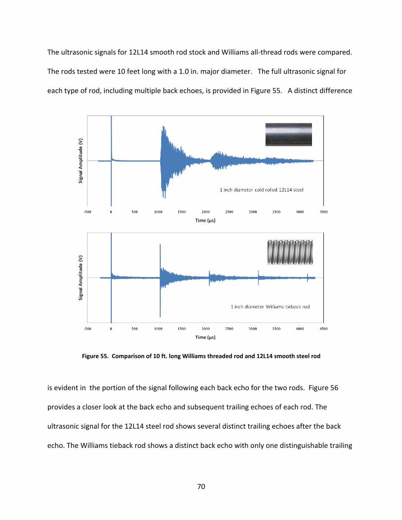
70 

 

The ultrasonic signals for 12L14 smooth rod stock and Williams all‐thread rods were compared. 

The rods tested were 10 feet long with a 1.0 in. major diameter.   The full ultrasonic signal for 

each type of rod, including multiple back echoes, is provided in Figure 55.   A distinct difference  

 

Figure 55.  Comparison of 10 ft. long Williams threaded rod and 12L14 smooth steel rod 

 

is evident in  the portion of the signal following each back echo for the two rods.  Figure 56 

provides a closer look at the back echo and subsequent trailing echoes of each rod. The 

ultrasonic signal for the 12L14 steel rod shows several distinct trailing echoes after the back 

echo. The Williams tieback rod shows a distinct back echo with only one distinguishable trailing 

 

71 

 

echo.  The time between the back echo and the trailing echo was difficult to measure in the 

Williams threaded rod due to increased noise in the ultrasonic signal.  Threads in the Williams 

rod cause dispersion of the ultrasonic wave due to spurious reflections from the threaded 

surfaces.  Since trailing echoes involve at least one reflection from the surface of the rod, 

detecting trailing echoes from a threaded surface proves to be difficult.  This implies that 

calculating the exact outer diameter of a threaded rod may not be possible using the time 

between trailing echoes (Δt).  An approximation of the diameter may be calculated using the Δt 

between the peaks, instead of the leading edge, of back echo and the first trailing echo. 

 

 Figure 56.  Trailing echo comparison for 12L14 smooth rod and Williams threaded rod 

 

72 

 

5.2 Projected Length of Rod to be Inspected 

The maximum specimen length available for the study was 10 ft. long.   Thus, a process was 

established to determine the maximum detectable rod length using the pulse‐echo method 

with the available commercial ultrasonic transducers.   Three rods, 1.0 ft., 3.0 ft., and 6.0 ft. in 

length, were cut from the same Williams 1.0 in. diameter tieback rod.   Each rod was tested 

with the pulse‐echo method using the Olympus NDT M1042 5 MHz magnetic transducer 

coupled to the end of the rod.  The attenuation of the ultrasonic signal was determined by  

 

Figure 57.  Rectified time domain signals for 1 ft., 3 ft. and 6 ft. long Williams rods 

 

73 

 

evaluating the peak values of successive back echoes in each rod.  A rectified A‐scan, which 

acquires the absolute value of the ultrasonic signal amplitude, including all detectable back 

echoes, was recorded (Figure 57).  The attenuation of the wave amplitude along the rod was 

defined by Equation 29 (Kolsky, 1963) 

 

     Equation 29 

 

where ao is the initial amplitude,  α is the coefficient of attenuation, and x is the distance along 

the rod.  The units of the coefficient of attenuation are Nepers (Np) per length, where a Neper 

is a dimensionless quantity.   The peak amplitude of each back echo was plotted with respect to 

the distance traveled (Figure 58.)  The best fit trend line was calculated and displayed with the  

 

 

Figure 58.  Signal attenuation for 1.0 ft., 3.0 ft., and 6.0 ft. long Williams rods. 

 

74 

 

equation and R2 value.   The attenuation coefficients (α) for the 1 ft., 3 ft., and 6 ft. rods were 

0.177 Np/ft., 0.120 Np/ft., and 0.096 Np/ft. respectively.  The differences in magnitude of α 

were due to scattering which occurred each time the ultrasonic wave reflected from an end of 

the rod.  When the ultrasonic wave traveled an equivalent 12 feet along the 1 ft. long rod, the 

wave reflected from an end surface 11 times.  For the 3 ft. and 6 ft. long rods, the same 12 ft. 

equivalent length included 3 and 1 end reflections respectively.  The results show a decrease in 

attenuation coefficient with a decrease in the number of end surface reflections.  Longer rods 

have fewer reflections resulting in a smaller attenuation coefficient.   

 Figure 55 shows that a 10 ft. long 1.0 in. diameter Williams tieback rod exhibits 4 distinct back 

echoes in the ultrasonic signal.  This shows that the pulse echo method using a 5 MHz probe 

could be used to detect a back echo in a 1.0 in. diameter 40 ft. long Williams tieback rod.   This 

was a conservative estimate since an actual 40 ft. rod would not include the attenuation from 

the multiple end reflections in the 10 ft. rod. 

5.3 Signal Attenuation for Williams Rods in Soil 

The effect of ultrasonic signal attenuation in soil was important for testing Williams commercial 

tieback rods.  The amount of energy transmitted into the surrounding medium during ultrasonic 

inspection of a tieback rod is dependent upon the properties of that medium.  Williams tieback 

rods with various surrounding media were tested to investigate the effect on signal 

attenuation.  Three sections of 3 ft. long Williams tieback rods were placed in plywood boxes 

with approximately 5.5 in. of cover in each direction.  An ultrasonic transducer was coupled to 

 

75 

 

one end of the tieback rod which protruded through the end of the box (Figure 59).  Each box 

was filled with one of three soils:  sand, loose soil, and compacted soil. 

      

Figure 59.  Boxes constructed for signal attenuation tests in soils 

5.3.1 Soil Characterization 

Two soils, sand and Palouse soil, were used in the tests.  The sand was collected from a quarry 

run by Atlas Concrete company in Lewiston, Idaho.  The Palouse soil was collected from topsoil 

in the Palouse region of Washington State.  The soils were characterized according to the 

protocol developed by the Army Corps of Engineers for earth retentions systems, including 

grain size distribution and Atterberg limit tests (US Army Corps of Engineers, 1994).    

A grain size distribution test was performed according to ASTM D422 (ASTM Standard D422, 

2007).  The results were plotted for each soil in Figure 60 and the coefficient of uniformity (Cu) 

and coefficient of curvature (Cc) were calculated for each soil.  The results were recorded in 

Table 12. 

 

76 

 

 

Figure 60.  Grain size distribution for sand and soil samples 

 

Table 12.  Soil characterization 

Type Coefficient of Uniformity 

     (Cu)Coefficient of Curvature 

    (Cc)

Sand  4.65 0.66

Palouse Soil  13.08 0.41

 

Atterberg limits tests were performed according to ASTM D4318 (ASTM Standard D4318, 2005).  

The Atterberg limits are a scaling system used to characterize the relationship between the 

water content of a soil and its physical behavior.  The liquid limit (LL), plastic limit (PL), plasticity 

index (PI), and the flow index for the Palouse soil were determined. Figure 61 shows the  

 

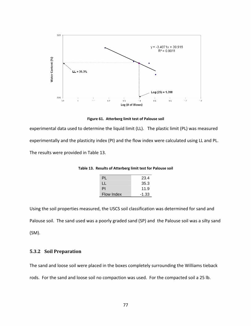
77 

 

 

Figure 61.  Atterberg limit test of Palouse soil 

experimental data used to determine the liquid limit (LL).   The plastic limit (PL) was measured 

experimentally and the plasticity index (PI) and the flow index were calculated using LL and PL. 

The results were provided in Table 13.   

Table 13.  Results of Atterberg limit test for Palouse soil 

PL 23.4LL 35.3PI 11.9Flow Index -1.33

 

Using the soil properties measured, the USCS soil classification was determined for sand and 

Palouse soil.  The sand used was a poorly graded sand (SP) and  the Palouse soil was a silty sand 

(SM). 

5.3.2 Soil Preparation 

The sand and loose soil were placed in the boxes completely surrounding the Williams tieback 

rods.  For the sand and loose soil no compaction was used.  For the compacted soil a 25 lb. 

 

78 

 

tamper with a 5 in. by 7 in. base plate was used to compact the soil.  The soil was compacted in 

3 in. layers.  Approximately 5 in. of soil was placed in the box without the tieback rod and 

compacted with approximately 15 blows per square foot.  After the second layer was 

compacted, the Williams tieback rod was positioned in the box.  Two more layers of soil were 

compacted on top of the tieback rod using the same compaction technique.   

Each soil was tested with two water contents.   The first test was performed using the original 

water content as it arrived on site, establishing the "baseline" water content.  After tests were 

performed with the "baseline" water content, water was added at a steady rate of 0.2 gallons 

per minute for 1 hour to saturate the soil.  The soil was allowed to drain for 24 hours before the 

second set of tests was performed. This was considered the "wet" condition.  Table 14 records 

the calculated water content for each soil condition according to ASTM D2216 (ASTM Standard 

D2216, 2005). 

Table 14.  Water content for each soil test 

Sand Loose Soil Compacted Soil

Baseline 5.28% 12.18% 12.18%

Wet 7.74% 28.21% 25.90%

5.3.3 Signal Attenuation for Tieback Rods in Soil 

Attenuation tests of 3.0 ft. sections of threaded Williams tieback rods were performed for the 

"baseline" and "wet" condition for each soil.   Control tests without any surrounding soil were 

also performed on each of the three rods.   The ultrasonic signal was recorded to determine the 

maximum number of detectable back echoes.  The maximum amplitude of each detectable 

 

79 

 

back echo was plotted, and an exponential decay trend line with R2 value was added (Figure 

62).  The exponent value represents the coefficient of attenuation for the signal with respect to  

 

Figure 62.  Exponential decay of back echo peaks in 3.0 ft. long Williams rod 

distance traveled. In order to evaluate repeatability, 10 signals were recorded for each soil, and 

the transducer was removed and reapplied after each measurement.  The coefficient of 

attenuation for each condition was averaged, and recorded in Table 15. The results show that 

there was no major change in attenuation due to the surrounding medium.  The control rods 

for sand, loose soil, and compact soil had an average coefficient of attenuation of 0.0803 Np/ft., 

0.0705 Np/ft., and 0.0883 Np/ft. respectively.  The discrepancy between each of the control 

rods was due to variations in the surface at the end of each rod.  An increase in surface 

roughness increases scattering during wave reflection.  For sand, the coefficients of attenuation 

were 0.0803 Np/ft., 0.0793 Np/ft., and 0.0817 Np/ft. for the control, "baseline", and "wet" 

samples.   There was no significant increase in attenuation from the control to the "baseline" or 

"wet" condition.  The "baseline" condition even had a coefficient lower than the control.  For 

 

80 

 

Table 15.  Attenuation coefficients of the ultrasonic signal for Williams tieback rods in soils 

Sand  Loose Soil Compacted Soil Control  Baseline  Wet  Control Baseline Wet  Control Baseline  Wet 0.081  0.075  0.078  0.072 0.069 0.065 0.095 0.076  0.0830.074  0.084  0.08  0.068 0.069 0.074 0.094 0.076  0.0820.084  0.083  0.087  0.066 0.073 0.073 0.083 0.079  0.0710.079  0.082  0.085  0.065 0.072 0.07 0.083 0.076  0.070.079  0.08  0.079  0.064 0.076 0.075 0.093 0.095  0.0890.083  0.08  0.078  0.077 0.075 0.067 0.081 0.09  0.0890.08  0.083  0.081  0.073 0.075 0.061 0.088 0.08  0.0830.079  0.073  0.081  0.073 0.073 0.073 0.089 0.081  0.0830.083  0.079  0.086  0.075 0.086 0.076 0.093 0.075  0.090.081  0.067  0.082  0.072 0.086 0.067 0.084 0.075  0.091

Average  Average  Average  Average Average Average Average Average  Average

0.0803  0.0793  0.0817  0.0705 0.0754 0.0701 0.0883 0.0803  0.0831

Std. Dev.  Std. Dev.  Std. Dev.  Std. Dev. Std. Dev. Std. Dev. Std. Dev. Std. Dev.  Std. Dev.0.0029  0.004  0.0033  0.0045 0.0061 0.0049 0.0053 0.0069  0.0074

CoV  CoV  CoV  CoV CoV CoV CoV CoV  CoV

0.0361  0.0504  0.0404  0.0638 0.0809 0.0699 0.0600 0.0859  0.0890

   z‐Test  z‐Test    z‐Test z‐Test   z‐Test  z‐Test

   0.640  ‐1.008    ‐2.044 0.190   2.908  1.807

 

the loose soil the coefficients of attenuations were 0.0705 Np/ft., 0.0754 Np/ft., and 0.0701 

Np/ft. for the control, "baseline", and "wet" samples.  Again, there was no significant increase 

in attenuation from the control to the "baseline" or "wet" condition.  For the compact soil the 

coefficients of attenuation were 0.0883 Np/ft., 0.0803 Np/ft., and 0.0831 Np/ft. for the control, 

"baseline", and "wet" samples. In this case the attenuation coefficients for the "baseline" and 

the "wet" condition were slightly less than the coefficient of attenuation for the control.   The z‐

Test for each "baseline" and "wet" test compared with the control showed that all tests, except 

the "baseline" for the compacted soil, were within a 99% confidence interval  (‐2.58 ≤ z ≤ 2.58).  

Normalized data is also shown in Table 16 which is calculated by dividing each of the "baseline" 

 

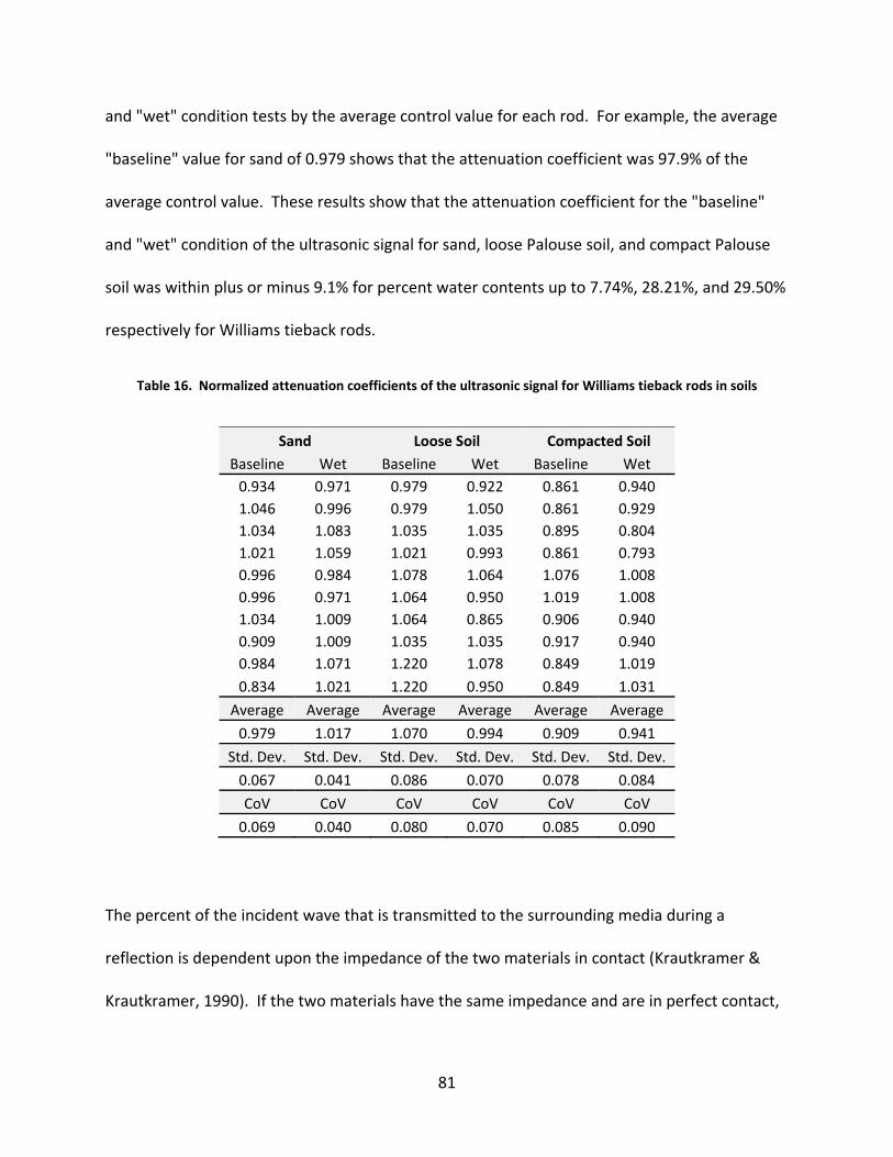
81 

 

and "wet" condition tests by the average control value for each rod.  For example, the average 

"baseline" value for sand of 0.979 shows that the attenuation coefficient was 97.9% of the 

average control value.  These results show that the attenuation coefficient for the "baseline" 

and "wet" condition of the ultrasonic signal for sand, loose Palouse soil, and compact Palouse 

soil was within plus or minus 9.1% for percent water contents up to 7.74%, 28.21%, and 29.50% 

respectively for Williams tieback rods.   

Table 16.  Normalized attenuation coefficients of the ultrasonic signal for Williams tieback rods in soils 

Sand  Loose Soil Compacted Soil Baseline  Wet  Baseline Wet  Baseline Wet  0.934  0.971  0.979 0.922 0.861 0.940 1.046  0.996  0.979 1.050 0.861 0.929 1.034  1.083  1.035 1.035 0.895 0.804 1.021  1.059  1.021 0.993 0.861 0.793 0.996  0.984  1.078 1.064 1.076 1.008 0.996  0.971  1.064 0.950 1.019 1.008 1.034  1.009  1.064 0.865 0.906 0.940 0.909  1.009  1.035 1.035 0.917 0.940 0.984  1.071  1.220 1.078 0.849 1.019 0.834  1.021  1.220 0.950 0.849 1.031 

Average  Average Average Average Average Average 0.979  1.017  1.070 0.994 0.909 0.941 

Std. Dev.  Std. Dev. Std. Dev. Std. Dev. Std. Dev. Std. Dev. 0.067  0.041  0.086 0.070 0.078 0.084 CoV  CoV  CoV CoV CoV CoV 0.069  0.040  0.080 0.070 0.085 0.090 

 

The percent of the incident wave that is transmitted to the surrounding media during a 

reflection is dependent upon the impedance of the two materials in contact (Krautkramer & 

Krautkramer, 1990).  If the two materials have the same impedance and are in perfect contact, 

 

82 

 

then all the energy will transfer through the boundary.  The transmittance percent for two 

dissimilar impedances is given by  

         Equation 30 

where Z1 is the impedance of the steel (Z = 46.0 MRayls) and Z2 is the impedance of the 

surrounding media, for the materials in this study.  Figure 63 shows the transmittance of a steel 

rod embedded in several  surrounding media including water (Z = 1.48 MRayls) and concrete (Z 

= 8.0 MRayls).  For a tieback rod in soil, part of the surrounding media is  air (Z = 0.000429 

MRayls), which drastically decreases the transmittance of the incident wave to the surrounding 

media.  Considering that a portion of the surrounding media is air and the first back echo only 

has one reflection, the transmittance is negligible.  Thus, the inspectable lengths of tieback rods 

will not vary when the rods are embedded in soils. 

 

Figure 63.  Transmittance for steel with water and concrete surrounding media 

 

83 

 

5.4 Actual Tieback Rods with Flaws 

Simulated corrosion was machined in 3 ft. Williams tieback rod sections to determine if specific 

geometries could be detected in commercial tieback rods.   These included location of 

simulated corrosion, diameter of simulated corrosion, length of simulated corrosion, and the 

transition of simulated corrosion. 

5.4.1 Location of Simulated Corrosion 

Three Williams steel rods, 3 ft. long and 1 in. in diameter, were machined with simulated 

corrosion at various locations to validate the pulse‐echo method for location the leading edge 

of simulated corrosion in a Williams tieback rod.  Simulated corrosion with a 0.5 in. diameter  

 

9.28 in. 

36 in. 

0.500 in. 1.00 in.

2.0 in.

15.97 in. 

36 in. 

0.500 in. 1.00 in.

2.0 in.

22.84 in. 

36 in. 

0.500 in. 1.00 in. 

2.0 in.

* Transducer was mounted on left end of the rod. 

* All transitions were 90° as shown at right 

90°

Figure 64.  3.0 ft. long 1.0 in. diameter Williams tieback rods with 2.0 in. length of 0.5 in. simulated corrosion diameter at 9.28 in., 15.97 in., and 22.84 in. along the rod  

 

84 

 

and  2.0 in. length was machined at 9.28 in., 15.97 in., and 22.84 in. along the length of the 

steel rods (Figure 64). The location of simulated corrosion was easily detectable based on the 

time between the main bang and the leading edge of the flaw echo.  The following signals 

(Figure 65) show a flaw echo appearing in the ultrasonic signal that correlates directly with the 

location of the flaw.  The formula for length (Equation 27) was used to determine the location 

of the flaw (Table 17) for each of the three rods in Figure 65.  The three rods showed a 

maximum percent difference of 1.59% between measured and calculated flaw location.    The 

 

Figure 65. Ultrasonic signals from 3.0 ft. long 1.0 in. diameter Williams tieback rods with 2.0 in. length of 0.5 in. diameter simulated corrosion at 9.28 in., 15.97 in., and 22.84 in. along the rod.  

 

 

85 

 

results show that the ability to locate the flaw position was not affected by the threads of the 

Williams rods. 

Table 17.  Comparison of measured and calculated location of simulated corrosion 

Measured Flaw Location (in.)   Flaw Time (µs) Calculated Flaw Location (in) % Difference9.28  79.3 9.13 1.59% 15.97  138.3 15.93 0.27% 22.84  197.4 22.73 0.47% 

 

5.4.2 Diameter of Simulated Corrosion 

To verify the detection of simulated corrosion diameter on Williams tieback rods, two 3 ft. long 

rods were machined with 0.5 in. diameter and 0.75 in. diameter simulated corrosion regions  

 

16.0 in. 

36 in. 

0.500 in. 1.00 in.

2.0 in.

* Transducer is mounted on left side of rod. 

* All transitions are 90° as shown at right 

90°

Figure 66.  3.0 ft. long 1.0 in. diameter Williams rods with 2.0 in. lengths of 0.5 in. and 0.75 in. diameter simulated corrosion 

16.0 in. 

36 in. 

0.750 in. 1.00 in.

2.0 in.

 

86 

 

 

Figure 67.  Comparison of Williams rods with 0.5 in. and 0.75in. diameter of simulated corrosion 

(Figure 66).   The first back echo with each distinguishable trailing echoes was provided in 

Figure 67.  The time between the trailing echoes was measured (Table 18.)  Using Equation 25 

the diameter was calculated from the spacing of the trailing echoes.  The 0.5 in. simulated 

corrosion diameter rod had a calculated diameter of 0.51 in. resulting in a 1.9% difference.   The 

0.75 in. simulated corrosion diameter rod had a calculated diameter of 0.73 resulting in a 2.6%  

difference.  This provides a very strong correlation between the minimum diameter (or 

simulated corrosion diameter) and the time between trailing echoes for the Williams rod.   

Table 18.  Time between trailing echoes for 0.5 in. and 0.75 in. simulated corrosion diameter 

Rod  Smallest Diameter (in.)

Measured Time (µs)

Calculated Diameter (in.) % Difference

0.5 in. Simulated Corrosion  0.50  3.34  0.51  1.9% 

0.75 in. Simulated Corrosion  0.75  4.79  0.73  2.6% 

 

87 

 

5.4.3 Length of Simulated Corrosion 

Two rods were machined with 2 in. and 8 in. lengths of simulated corrosion to investigate the 

length of simulated corrosion in Williams rods.  The 0.5 in. simulated corrosion diameter was 

machined in 3 ft. lengths of 1 in. diameter Williams rods starting at 9.0 in. from the end  

 

(Figure 68).  An FFT was taken of the back echo for each rod.  The results (Figure 69) show that 

the peak frequency for the 2in. and 10 in. length of simulated corrosion lies between the 0.5 in. 

diameter and 1.0 in. diameter 3.0 ft. long rod of 12L14 steel.   This shows that the threaded rod 

does not affect the frequency content  of the back echo.  The amplitude of the back echo and 

first trailing echo were also recorded for each rod.  The ratio of the first trailing echo to the 

back echo was calculated and plotted with the data for the 12L14 rods with simulated corrosion 

(Figure 70).  The ratio for the 2.0 in. and 10.0 in. long simulated corrosion was 1.147 and 2.050, 

9.0 in. 

36 in. 

0.500 in. 1.00 in.

2.0 in.

9.0 in. 

36 in. 

0.500 in. 1.00 in. 

10.0 in.

Figure 68.  3.0 ft. long 1.0 in. diameter Williams tieback rods with 2.0 in. and 10.0 in. lengths of 0.5 in. diameter simulated corrosion  

* Transducer is mounted on left side of rod. 

* All transitions are 90° as shown at right 

90°

 

88 

 

respectively.  This was comparable to the 0.972 and 2.307 values for the 12L14 rod with 2.0 in. 

and 10.0 in. simulated corrosion respectively. 

 Figure 69.  Frequency of ultrasonic signal of Williams rods with 2.0 in and 8.0 in. lengths of simulated corrosion. 

 

Figure 70.  Ratio of trailing echo and back echo for 2.0 in. and 10.0 in. long simulated corrosion in 3.0 ft. long Williams rods 

 

89 

 

5.4.4 Transition of Simulated Corrosion 

Finally, a 3 ft. long Williams rod was machined with a 0.5 in. simulated corrosion diameter and a 

45° transition angle (Figure 71).  This rod was used to investigate the ability to detect the 

location, diameter, and length of simulated corrosion for a rod with a 45° transition angle in a 

Williams rod.   The full ultrasonic signal from the pulse‐echo test was recorded for the Williams 

rod with a 45° transition (Figure 72).  The signal shows a distinct flaw and back echo.  The flaw 

and back echo were each followed by four distinct trailing echoes.   

 

 

Figure 72.  Full ultrasonic signal for 2 in. length of 0.5 in. diameter simulated corrosion with 45° transition angle for Williams tieback rod  

* Transducer is mounted on left side of rod. 

45o

36 in. 

15.75 in.   0.500 in. 1.00 in.

2.0 in.

Figure 71.  Rod used for simulated corrosion detection with a 45° transition angle  

 

90 

 

 

The arrival time of the flaw echo was 138.7 µs.  Using the longitudinal wave speed of the 75 ksi 

steel, the flaw location was calculated to be 15.97 in, which has a 1.41% difference from the 

measured 15.75 in. to the beginning of the transition of the flaw (Table 19).  This shows that the 

method used in the previous chapter for locating the position of simulated corrosion can be 

used in Williams rods with a 45° transition angle.   

Table 19.  Calculated simulated corrosion location for Williams rod with 45° transition angle 

Measured Flaw Location (in.)   Flaw Time (µs) Calculated Flaw Location (in) % Difference

15.75  138.7 15.97 1.41% 

 

The back echo and subsequent trailing echoes were recorded for the Williams rod with a 45˚

transition angle.  The back echo and four trailing echoes were visible (Figure 73.)  The arrival 

time of the first back echo and two trailing echoes were used to calculate the time between 

echoes.  This time between trailing echoes was used to calculate the diameter of the simulated 

 

Figure 73.  First back echo and successive trailing echoes for 2 in. simulated corrosion with 45° transition   

 

91 

 

corrosion according to Equation 25 (Table 20).  The calculated diameter was 0.502 in. which had 

a 0.4% difference from the measured value of 0.500 in.  This shows that the method for 

detecting the diameter of simulated corrosion can be used for Williams rods with a 45° 

transition angle. 

Table 20.  Comparison of measured and calculated diameter of simulated corrosion for Williams rod with 45° transition angle 

Rod  Smallest Diameter (in.) 

Measured Time (µs) 

Calculated Diameter (in.)  % Difference 

0.5 in. simulated corrosion 0.500 3.27 0.502 0.4% 

 

The FFT of the first back echo was recorded for the Williams rod with a 2 in. length of simulated 

corrosion and a 45° transition angle.  The result was plotted with the FFT signals from a 0.5 in. 

diameter and 1.0 in. diameter 3.0 ft. long rods of 12L14 steel.  The results show that the 

Figure 74. Frequency of back echo of 2 in. long 0.5 in. diameter simulated corrosion with 45° transition in Williams rod 

 

92 

 

frequency domain for the Williams rod with a 45° transition lies between the frequency domain 

for the 0.5 in. and 1.0 in. rod.  The frequency domain of the ultrasonic signal for the Williams 

rod with simulated corrosion has two major peaks as compared to the single peaks for the rods 

without any corrosion. 

The amplitude of the back echo and first trailing echo were also recorded.  The ratio of the first 

trailing echo to the back echo was calculated and plotted with the data for the 12L14 rods with 

simulated corrosion (Figure 75).  The ratio for the 2.0 in. long simulated corrosion with a 45° 

transition was 0.865.  There was an 11%  difference from the 0.972 value for the 12L14 rod. 

 

 

Figure 75.  Ratio of trailing echo and back echo for 2.0 in. simulated corrosion length with 45° transition in 3.0 ft. long  Williams rods 

   

 

93 

 

6 Inspection Procedures 

This chapter outlines the recommended procedures for inspecting steel tieback rods for 

corrosion in the field.  The tests performed in the previous sections involved simulated 

corrosion of steel tieback rods.  Inspection of rods in the field would involve rods with actual 

corrosion.  Actual corrosion incorporates a rough surface in the corroded region as opposed to 

the smooth surfaces of simulated corrosion.  The following guidelines consider these 

differences in developing inspection procedures for field testing.    

6.1 Inspection of Simulated Corrosion 

The research performed at Washington State University identified methods to determine the 

location and diameter of simulated corrosion on 1.0 in. diameter 12L14 steel rods and 1.0 in. 

diameter Williams steel all‐thread tieback rods.  Figure 76 depicts the full ultrasonic signal for a  

 Figure 76 Ultrasonic pulse‐echo signal for 12L14 smooth steel rod and Williams steel all‐thread tieback rod both 

with simulated corrosion  

12L14 Steel Rod 

Williams Tieback Rod 

 

94 

 

3.0 ft. long 1.0 inch diameter 12L14 smooth surface rod and a Williams commercial tieback rod 

both with a 2.0 in. long section of 0.5 in. diameter simulated corrosion starting 9.0 in. from the 

left end.  Older construction practices included smooth A36 steel rods with upset threads at 

either end, and current practices use Williams, DWYIDAG, SAS or Con‐Tec all‐thread rods.  The 

location of the simulated corrosion can be identified from the ultrasonic signal.  If the length is 

known, any echo that appears before the back echo is evidence of corrosion, cracking, or some 

other flaw.  The location of a flaw is calculated based on the time between the "main bang" and 

the "flaw echo".  The length, L, from the transducer to the leading edge of simulated corrosion 

can be calculated using Equation 30  where C1 is the bulk longitudinal wave speed of the  

·        Equation 31 

material and t is the time between the main bang and the leading edge of the flaw echo.   The 

typical value for the longitudinal wave speed in steel is C1 = 19,190 ft/s.   The time, t, is  

 Figure 77.  Location of the leading edge for the main bang and flaw echo 

 

95 

 

measured from the leading edge of the main bang to the leading edge of the flaw echo.  The 

leading edge for each echo is defined as the first point that appears outside the bounds of the 

signal noise.  Figure 77 plots each point of the ultrasonic signal in the range of the main bang 

and the flaw echo to identify the leading edge.  For rods with a transition from the original 

diameter to the flaw diameter, the measured time may include a delay from the actual flaw 

location.   The maximum delay for a 5° transition angle in a 1.0 in. diameter rod with 0.5 in. 

diameter simulated corrosion was 23.8 µs, which corresponds to an error of 0.44 in. for 

determining the location of the flaw.   

Figure 78 depicts the back echo and trailing echoes for a 3.0 ft. long 1.0 inch diameter 12L14 

smooth surface rod and a Williams commercial tieback rod, both with a 2.0 in. long section of 

0.5 in. diameter simulated corrosion starting 17.0 in. from the left end of the rod.  The time 

between the trailing echoes following the first back echo can be directly related to the diameter  

 

 Figure 78.  First back echo and subsequent trailing echoes for inspection of simulated corrosion diameter 

inspection in 1.0 in. diameter 12L14 steel rod and 1.0 in. diameter Williams rod 

12L14 Steel Rod 

Williams Tieback Rod 

 

96 

 

of simulated corrosion.  Equation 31 correlates the diameter of the rod (d) to the time between 

echoes (∆t), based upon the speed of longitudinal wave propagation (C1) and the speed of 

transverse wave propagation (C2).   The time between trailing echoes is measured in the same  

∆         Equation 32 

manner as the time between the main bang and the flaw echo.  The individual points of each 

echo are plotted to identify the leading edge which is the first point to raise above or below the 

noise of the signal.   Typical values for the longitudinal and shear wave speed in steel are C1 = 

19,190 ft/s and C2 = 10,597 ft/s.  The diameter of simulated corrosion can be used in 

conjunction with the original diameter to determine the reduction in load capacity.  Equation 

32 depicts the percent load capacity for a  rod with simulated corrosion.    

%            Equation 33 

 

The load capacity is dependent upon the diameter of the corroded region, dc, and the original 

rod diameter, do.  The ability to identify the location and diameter of corrosion provides an 

inspector with the ability to approximate the structural integrity of a tieback rod.   

The selection of the ultrasonic transducer is critical when inspecting a tieback rod.  The main 

variables  to consider in commercial transducers are the diameter of the transducer and the 

frequency of the ultrasonic signal generated.    The transducer diameter should be as large as 

possible without exceeding the diameter of the rod.  An increase in the diameter of the 

 

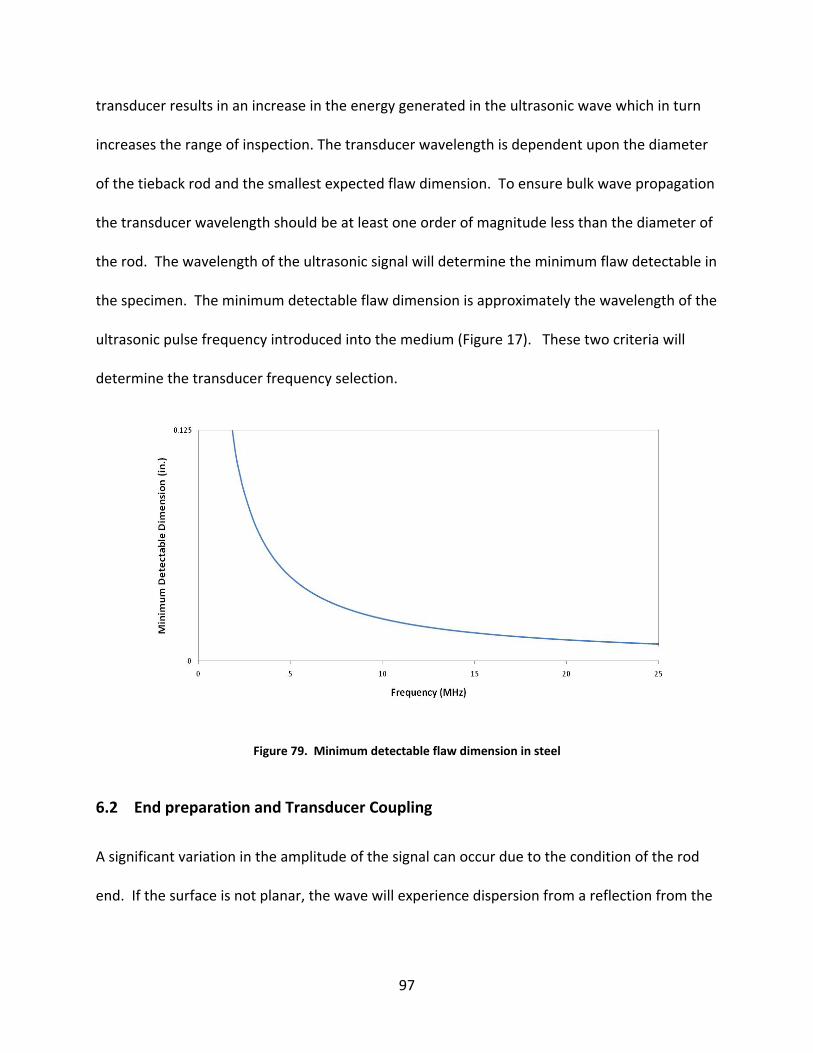
97 

 

transducer results in an increase in the energy generated in the ultrasonic wave which in turn 

increases the range of inspection. The transducer wavelength is dependent upon the diameter 

of the tieback rod and the smallest expected flaw dimension.  To ensure bulk wave propagation 

the transducer wavelength should be at least one order of magnitude less than the diameter of 

the rod.  The wavelength of the ultrasonic signal will determine the minimum flaw detectable in 

the specimen.  The minimum detectable flaw dimension is approximately the wavelength of the 

ultrasonic pulse frequency introduced into the medium (Figure 17).   These two criteria will 

determine the transducer frequency selection. 

 

Figure 79.  Minimum detectable flaw dimension in steel  

6.2 End preparation and Transducer Coupling 

A significant variation in the amplitude of the signal can occur due to the condition of the rod 

end.  If the surface is not planar, the wave will experience dispersion from a reflection from the 

 

98 

 

end of the rod.   Another source of amplitude loss can occur in the coupling of the transducer to 

the rod.  It is imperative to have a smooth planar surface to attach the transducer.  Thus, it may 

be necessary to cut a new surface at the end of the rod.   Also, contaminants located between 

the transducer and the end of the rod may result in poor transfer of energy to the rod.  

Therefore, the end of each rod must be cleaned, and a couplant gel applied before the 

transducer is coupled to the end of the rod.   Without the gel, the transducer will not effectively 

couple the ultrasonic signal into the rod, resulting in an extremely poor ultrasonic wave, if any 

at all.   A magnetic transducer is also recommended to provide a consistent adhering force 

between the transducer and the end of the rod. 

6.3 Commercial Tieback Rod Testing 

The following guidelines are presented to assist in developing an inspection procedure for 

tieback rods in the field.  Transitioning from testing smooth 12L14 samples to in‐situ testing of 

commercial tieback rods  introduces several potential limitations.    First, turnbuckles are often 

used when a design calls for rods longer than 50 ft.  An ultrasonic signal is not able to propagate 

through the turnbuckle, thus only the first section of rod is inspectable.  Second, actual 

corrosion will not have a smooth surface, or a single diameter.  The irregular surface of actual 

corrosion will increase scattering of the ultrasonic wave during reflection.   Third, curvature in 

the tieback rod may eliminate the detection of the back echo. If a direct line of sight through 

the rod from the front to the back of the rod is eliminated then detection of a direct back echo 

is not possible.  These factors may limit the effectiveness of ultrasonic inspection in some 

scenarios.    The following charts provide guidelines for the use of the ultrasonic pulse‐echo 

 

99 

 

method for inspecting tieback rods.   The guidelines are divided into two sections.  The first 

section covers inspections of new construction.  These guidelines assume that initial ultrasonic 

pulse‐echo measurements will be performed after the placement of the rods and prior to the 

facade construction, which covers the ends of the tieback rods.  The second section covers 

inspection of existing construction.  This section is divided into two sections.  The first sub‐

section includes tieback rod lengths that are recorded in the design plans.  The second  section 

is for inspection of tieback rods with unknown length. 

 

6.3.1 New Construction 

This section introduces inspection guidelines for tieback rods in new construction.  Performing 

several measurements during the construction can significantly increase the ability to monitor 

corrosion in steel tieback rods.  An ultrasonic pulse‐echo measurement performed after the 

placement of the rods, and prior to the façade construction generates a "control signal" to 

compare with subsequent measurements during the life of the rod.   The control signal should 

include two separate inspections.  First, a full signal showing all detectable back echoes, and 

second the first back echo with all detectable trailing echoes.  The full signal can be used to 

calculate the actual longitudinal wave speed of each rod, using the time between the main 

bang and the first back echo.  A published value for the shear wave speed, C2 = 10,597 ft/s will 

be used.  The following is a series of steps to aid in future inspections: 

 

 

100 

 

Step #1:  Calculate the longitudinal wave speed from the "control signal" 

Determine the time between the main bang and the first back echo from the control signal.  

Using the rod length and Equation 30 calculate the longitudinal wave speed. 

Step #2: Perform a pulse‐echo inspection on the tieback rod 

Record three different sections of the ultrasonic signal.  First, record the full signal, extending to 

the first back with all detectable trailing echoes.  Second, record the back echo with all 

detectable trailing echoes.  Third, record any flaw echo and all detectable trailing echoes that 

appear before the back echo.   

Step #3:  Compare the "control signal" with the full ultrasonic signal from the inspection 

Note any differences between the "control signal" and the inspection  signal recorded in Step 

#1.  Any echo that appears before the back echo represents a flaw in the rod.   Also, any 

variation in the amplitude of the back echo or subsequent trailing echoes can represent the 

growth of a flaw, or bending of the tieback rod. 

Step #4:  Verify the length of the tieback rod 

Measure the time between the main bang and the back echo.  Use this measurement to 

calculate the length of the rod, using the longitudinal wave speed from Step #1 with Equation 

30.  Compare the calculated rod length with the original rod length to ensure that there are no 

complete breaks in the rod. 

 

 

101 

 

Step #5:  Verify the outer diameter of the tieback rod 

If a flaw echo does not exist, calculate the time between trailing echoes after the back echo.  If 

a flaw echo exists, calculate the time between trailing echoes after the flaw echo.  Using the 

appropriate time between trailing echoes, the longitudinal wave speed from Step #1, a shear 

wave speed of 10,597 ft/s and Equation 31 to calculate the diameter of the rod. The original 

diameter of the rod should be visible from the exposed end of the tieback rod.  The calculated 

diameter and the original diameter should be approximately the same.  Measuring the time 

between trailing echoes may be difficult for threaded rods, because the threads cause 

dispersion of the ultrasonic wave when it mode converts and reflects from the outer diameter 

to create the trailing echoes. 

Step #6:  Calculate the location of the flaw (if a flaw echo exists) 

Measure the time between the main bang and the first flaw echo.  Use this measurement to 

calculate the distance to the flaw, using the longitudinal wave speed from Step #1 with 

Equation 30.   Repeat this step for each distinct flaw echo.  Be careful not to mistake a second 

flaw echo as an additional.  An echo that appears at twice the distance of the first flaw is most 

likely a second flaw echo and not an additional flaw.   

Step #7 Determine the minimum diameter of the tieback rod (if a flaw exists) 

Measure the time between the back echo and the first trailing echo.  Use this measurement to 

calculate the minimum diameter of the rod, using the longitudinal wave speed calculated in 

Step #1, and a shear wave speed of 10,597 ft/s  with Equation 30.    

 

102 

 

6.3.2 Existing Construction 

Interpretation of inspection of existing construction is more difficult than new construction.  

Since there is not a control signal generated during the construction process, these guidelines 

must be divided into two sub‐categories.  The first approach assumes that the original plans are 

available which identify the original rod length.  The second approach is for inspection of rods 

of unknown length.    

6.3.2.1 Original rod length is known 

Rods with a known length provide dimensions to identify the back echo in the ultrasonic signal.  

The following is series of steps to aid in inspection of tieback rods of known length: 

Step #1:  Calculate the time between the main bang and the back echo 

Using the length of the rod and a longitudinal wave speed of C1 = 19,190 ft/s calculate the 

expected time between the main bang and the back echo using Equation 30. 

Step #2: Perform a pulse‐echo inspection on the tieback rod 

Record three different sections of the ultrasonic signal.  First, record the full signal, extending to 

the first back with all detectable trailing echoes.  Use the expected time from the main bang to 

the trailing echo from Step #1 to approximate the time window necessary to capture the entire 

signal.  Second, record the back echo with all detectable trailing echoes.  Third, record any flaw 

echo that appears before the back echo and all detectable trailing echoes.   

 

 

103 

 

Step #3:  Verify the length of the tieback rod 

Measure the time between the main bang and the back echo in the ultrasonic signal.  Use this 

measurement to calculate the length of the rod, using a longitudinal wave speed of C1 = 19,190 

ft/s with Equation 30.  Compare the calculated rod length with the original rod length to ensure 

that there are no complete breaks in the rod. 

Step #4:  Verify the outer diameter of the tieback rod 

If a flaw echo does not exist, calculate the time between trailing echoes after the back echo.  If 

a flaw echo exists, calculate the time between trailing echoes after the flaw echo.  Using the 

appropriate time between trailing echoes and Equation 31, calculate the diameter of the rod.   

Measuring the time between trailing echoes may be difficult for threaded rods, because the 

threads cause dispersion of the ultrasonic wave when it reflects and mode converts from the 

outer diameter to create the trailing echoes. 

Step #5:  Calculate the location of the flaw (if a flaw echo exists) 

Measure the time between the main bang and the first flaw echo.  Use this measurement to 

calculate the distance to the flaw, using a longitudinal wave speed of C1 = 19,190 ft/s with 

Equation 30.   Repeat this step for each distinct flaw echo.  Be careful not to mistake a second 

flaw echo as second flaw.  An echo that appears at twice the distance of the first flaw is most 

likely a second flaw echo and not a second flaw.   

 

 

104 

 

Step #6 Determine the minimum diameter of the tieback rod (if a flaw exists) 

Measure the time between the back echo and the first trailing echo.  Use this measurement to 

calculate the minimum diameter of the rod, using the longitudinal wave speed of C1 = 19,190 

ft/s, and a shear wave speed of C2 = 10,597 ft/s  with Equation 30.    

6.3.2.2 Unknown length of rod 

A rod with unknown length requires a close inspection of the trailing echoes to identify possible 

flaws in the rod.   The following is series of steps to aid in inspection of tieback rods of unknown 

length: 

Step #1: Perform a pulse‐echo inspection on the tieback rod 

Record three different sections of the ultrasonic signal.  First, record the full signal, including all 

detectable echoes.  Second, record the furthest echo with all detectable trailing echoes.  Third, 

record any other echo that appears in the signal with  all detectable trailing echoes.   

Step #2: Determine if no detectable flaws are present 

Measure the time between trailing echoes for each echo recorded.  Using the time between 

trailing echoes, a longitudinal wave speed of C1 = 19,190 ft/s, a shear wave speed of 10,597 ft/s 

and Equation 31 calculate a diameter for each set of trailing echoes.  If the corresponding 

diameter for the first two sets of trailing echoes is approximately equal to the original diameter 

of the rod, then the echoes represent the first and second back echoes.  Since no flaw echoes 

 

105 

 

appear between the main bang and the first back echo, there are no detectable flaws in the 

rod. 

Step #3:  Identify the minimum diameter in the tieback rod 

If any of the diameters calculated in Step #2 are less than the original diameter, then there is a 

flaw present in the rod.   The minimum diameter calculated may not be the actual minimum 

diameter of the rod, because the signal may have reflected from a crack in the rod, or the flaw 

that represents a smaller diameter in the rod.  Without knowing the length of the rod, 

determining the absolute minimum diameter is impossible.  

Step #4:  Calculate the partial length of rod inspected for minimum diameter 

The partial length inspected for simulated corrosion can be calculated using the second to last 

echo detected.  The second to last echo represents the last reduced diameter that the 

ultrasonic wave traveled through before returning to the transducer.  Record the time between 

the main bang and the second to last echo.  Use this measurement to calculate the inspected 

length of rod using a longitudinal wave speed of C1 = 19,190 ft/s with Equation 30. 

   

 

106 

 

7 Summary and Conclusions 

This dissertation concentrated on the detection of simulated corrosion in steel tieback rods.   

Ultrasonic signals were used to determine the physical geometry of 0.25 in., 0.50 in., and 0.75 

in. diameter simulated corrosion in 1.0 in. diameter steel rods.  Research was also performed to 

investigate the use of ultrasonic waves in Williams commercial tieback rods.  Guidelines were 

developed for inspecting tieback rods with actual corrosion in field applications. 

The location, diameter, length, and transition of concentric simulated corrosion were 

investigated for straight steel rods.  For a 90° transition angle, the location of simulated 

corrosion was detectable based upon the time between the main bang and the flaw echo in the 

ultrasonic signal and the longitudinal wave speed of the steel.  A decrease in the transition 

angle results in a delay in the arrival time of the flaw echo.  The largest delay was 23.8 µs for 

the 5° transition which represents a potential error of 5.5 in. when estimating the location. 

The minimum diameter of concentric simulated corrosion in a straight rod was detectable 

based upon the distance between the back echo and the first trailing echo, and the longitudinal 

and shear wave speeds of the steel in accordance with previous research by Light & Joshi (Light 

& Joshi, 1987).   The time between the back echo and first trailing echo is exclusively dependent 

upon the minimum diameter of the rod, and is not dependent upon the transition angle of the 

simulated corrosion. 

The length of concentric simulated corrosion in a straight rod was detectable based on two 

different techniques.  First, an increase in the peak frequency of the back echo correlated with 

 

107 

 

an increase in the length of simulated corrosion.  Second, the ratio of the amplitude of the first 

trailing echo and the back echo correlated with an increase in the length of simulated 

corrosion.   

The investigation of the transition of the simulated corrosion concluded that the flaw echo is 

detectable for abrupt transitions of 90° down to as small as 5°.  The flaw echo experienced a 

decrease in amplitude below a 80° transition angle but was still detectable.  Two peaks were 

evident at  transition angles of 27.5° and 45°.  These peaks correlate to a shear and longitudinal 

wave reflection directly across the rod from the transition surface. 

Williams all‐thread tieback rods were investigated including projected detectable rod length, 

signal attenuation due to surrounding media, and simulated corrosion in tieback rods.  The 

signals in tieback rods showed a distinct back echo, with low signal amplitude following, due to 

the dispersion of the wave from the threads.  Since the back echo did not reflect from the 

threads, the amplitude was not affected.  The signal attenuation tests revealed that there was 

no significant amplitude loss in the back echo for sand, loose soil, or compact soil.  A projected 

detectable rod length was found to be 40 feet with the pulse‐echo method.  Finally, simulated 

corrosion in Williams tieback rods showed that location and diameter of simulated corrosion 

were detectable in threaded rods with a 90° and a 45° transition angle.  

The work presented in this dissertation forms original research that contributes to the following 

fields: 

1. Safety of structures within the field of Civil Engineering 2. Adding to the current literature of NDT testing  

 

108 

 

These contributions include: 

1. Effect of transitions on the ultrasonic signal 2. Effect of length of corrosion on the ultrasonic signal 3. Effect of soil on tieback rod signal attenuation 4. Detection of simulated corrosion in Williams tieback rods 

Based on the research presented, the following recommendations were made for future 

research.   

1. Investigate the minimum detectable cross‐section loss in 1.0 in. diameter tieback rods. 

For example, machine rods with 0.8125 in., 0.875 in, 0.9375 in. diameter of simulated 

corrosion and identify the smallest simulated corrosion that exhibits a flaw echo. 

2. Investigate the detectability of simulated corrosion in larger diameter tieback rods.  For 

example, machine simulated corrosion in 2.0 in. and 3.0 in. diameter Williams rods, and 

identify the detectable geometries. 

3. Investigate the detectability of additional geometric characteristics of simulated 

corrosion on the ultrasonic signal for the pulse‐echo method.  For example:  

• machine simulated corrosion with a variation in diameter in the corroded region, 

instead of uniform reduced diameter. 

• machine non‐concentric loss of cross‐section in steel rods. 

4. Investigate the detection of ultrasonic signals in rods with curvature to mimic rods that 

have bent during settlement.  Bend multiple commercial tieback rods to various radii 

and monitor the ultrasonic signal. 

 

109 

 

5. Investigate the effect of various thread characteristics on the ultrasonic signal using 

commercial tieback rods from a variety of manufacturers.  Include all‐thread rods from 

DWYIDAG, SAS and Con‐Tec. 

6. Investigate in situ testing to establish “control signals” for tieback rods in new or existing 

construction, followed by periodic monitoring to assess changes in the ultrasonic signal 

that occur due to field conditions over time. 

7. Investigate multiple simulated corrosion regions in the same rod.   For example, 

machine rods with multiple lengths of 0.5 in. diameter simulated corrosion in the same 

rod, or multiple lengths of 0.5 in. and 0.75 in. diameters. 

8. Investigate the detectability of actual corrosion in steel rods on the ultrasonic signal.  

Use accelerated‐corrosion in salt spray chambers to induce corrosion. 

   

 

110 

 

References Cited: 

ASTM Standard A108. (2007). Standard Specification for Steel Bar, Carbon and Alloy, Cold‐Finished , DOI: 10.1520/A0108‐07 . West Conshohocken, PA: ASTM International. 

ASTM Standard A29. (2005). Standard Specification for Steel Bars, Carbon and Alloy, Hot‐Wrought, General Requirements for , DOI: 10.1520/A0029_A0029M‐05 . West Conshohocken, PA: ASTM International. 

ASTM Standard A615. (2008). Standard Specification for Deformed and Plain Carbon‐Steel Bars for Concrete Reinforcement , DOI: 10.1520/A0615_A0615M‐08B . West Conshohocken, PA: ASTM International. 

ASTM Standard D2216. (2005). Standard Test Methods for Laboratory Determination of Water (Moisture) Content of Soil and Rock by Mass , DOI: 10.1520/D2216‐05 . West Conshohocken, PA: ASTM International. 

ASTM Standard D422. (2007). Standard Test Method for Particle‐Size Analysis of Soils , DOI: 10.1520/D0422‐63R07 . West Conshohocken, PA: ASTM International. 

ASTM Standard D4318. (2005). Standard Test Methods for Liquid Limit, Plastic Limit, and Plasticity Index of Soils , DOI: 10.1520/D4318‐05 . West Conshohocken, PA: ASTM International. 

Beard, M., Lowe, M., & Cawley, P. (2001). Inspection of Rockbolts using Guided Ultrasonic Waves. Review of Progress in Quantitative Nondestructive Evaluation , 1156‐1163. 

Bray, D. E., & Stanley, R. K. (1989). Nondestructive Evaluation. New York: CRC Press. 

Davies, R. (1948). A Critical Study of the Hopkinson Pressure Bar. Phil. Transactions , 375‐457. 

Esser, A. J., & Dingeldein, J. E. (2007). Failure of Tieback Wall Anchors Due to Corrosion. Geo‐Denver 2007, (pp. 1‐10). Denver. 

Hudson, G. (1943). Dispersion of Elastic Waves in Solid Circular Cylinders. Physics Review , 46‐51. 

Kolsky, B. (1963). Stress Waves in Solids. New York: Dover Publications Inc. 

Krautkramer, J., & Krautkramer, H. (1990). Ultrasonic Testing of Materials. Berlin: Springer‐Verlag. 

Light, G. M., & Joshi, N. R. (1987). Ultrasonic Waveguide Technique for Detection of Simulated Corrosion Wastages. Nondestructive Testing Communications , 13‐27. 

Main, L. G. (1988). Vibrations and Waves in Physics. New York: Cambridge University Press. 

Niles, G. B. (1996). In Situ Method for Inspecting Anchor Rods for Section Loss Using the Cylindrically Guided Wave Technique. IEEE Transactions of Power Delivery , 1601‐1605. 

 

111 

 

Pochhammer, J. (1876). About the reproduction speeds of small vibrations in an infinite isotropic circular cylinder. Journal of Pure and Applied Math , 324‐336. 

Pollock, D. G. (1997). Reliability Assessment of Timber Connections Through Ultrasonic Inspection of Bolts. Texas A&M University. 

US Army Corps of Engineers. (1994, March 31). Retrieved January 18, 2009, from Design of Sheet Pile Walls: http://140.194.76.129/publications/eng‐manuals/em1110‐2‐2504/ 

Williams Form Engineering Corp. (2008). Retrieved April 2, 2009, from Tie Rod Information: http://www.williamsform.com/