Ultra-large field-of-view two-photon microscopy

Ultra-large field-of-view two-photon microscopy

Philbert S. Tsai,1 Celine Mateo,1 Jeffrey J. Field,2 Chris B. Schaffer,3 Matthew E. Anderson,4 and David Kleinfeld1,5,*

1Department of Physics, University of California at San Diego, La Jolla, California, USA 2Department of Electrical & Computer Engineering, Colorado State University, Fort Collins, Colorado, USA

3Department of Biomedical Engineering, Cornell University, Ithaca, New York, USA 4Department of Physics, San Diego State University, San Diego, California, USA

5Section of Neurobiology, University of California, La Jolla, California, USA *[email protected]

Abstract: We present a two-photon microscope that images the full extent of murine cortex with an objective-limited spatial resolution across an 8 mm by 10 mm field. The lateral resolution is approximately 1 µm and the maximum scan speed is 5 mm/ms. The scan pathway employs large diameter compound lenses to minimize aberrations and performs near theoretical limits. We demonstrate the special utility of the microscope by recording resting-state vasomotion across both hemispheres of the murine brain through a transcranial window and by imaging histological sections without the need to stitch.

©2015 Optical Society of America

OCIS codes: (170.0170) Medical optics and biotechnology; (120.0120) Instrumentation, measurement, and metrology; (180.0180) Microscopy.

References and links

1. D. A. Leopold, Y. Murayama, and N. K. Logothetis, “Very slow activity fluctuations in monkey visual cortex: Implications for functional brain imaging,” Cereb. Cortex 13(4), 422–433 (2003).

2. S. Ogawa, T.-M. Lee, A. S. Nayak, and P. Glynn, “Oxygenation-sensitive contrast in magnetic resonance image of rodent brain at high magnetic fields,” Magn. Reson. Med. 14(1), 68–78 (1990).

3. M. D. Fox and M. E. Raichle, “Spontaneous fluctuations in brain activity observed with functional magnetic resonance imaging,” Nat. Rev. Neurosci. 8(9), 700–711 (2007).

4. J. M. Palva and S. Palva, “Infra-slow fluctuations in electrophysiological recordings, blood-oxygenation-level-dependent signals, and psychophysical time series,” Neuroimage 62(4), 2201–2211 (2012).

5. M. L. Schölvinck, A. Maier, F. Q. Ye, J. H. Duyn, and D. A. Leopold, “Neural basis of global resting-state fMRI activity,” Proc. Natl. Acad. Sci. U.S.A. 107(22), 10238–10243 (2010).

6. P. J. Drew, A. Y. Shih, and D. Kleinfeld, “Fluctuating and sensory-induced vasodynamics in rodent cortex extend arteriole capacity,” Proc. Natl. Acad. Sci. U.S.A. 108(20), 8473–8478 (2011).

7. J. H. Lee, R. Durand, V. Gradinaru, F. Zhang, I. Goshen, D. S. Kim, L. E. Fenno, C. Ramakrishnan, and K. Deisseroth, “Global and local fMRI signals driven by neurons defined optogenetically by type and wiring,” Nature 465(7299), 788–792 (2010).

8. P. P. Mitra, S. Ogawa, X. Hu, and K. Uğurbil, “The nature of spatiotemporal changes in cerebral hemodynamics as manifested in functional magnetic resonance imaging,” Magn. Reson. Med. 37(4), 511–518 (1997).

9. W. Denk, J. H. Strickler, and W. W. Webb, “Two-photon laser scanning fluorescence microscopy,” Science 248(4951), 73–76 (1990).

10. K. Svoboda, W. Denk, D. Kleinfeld, and D. W. Tank, “In vivo dendritic calcium dynamics in neocortical pyramidal neurons,” Nature 385(6612), 161–165 (1997).

11. F. Helmchen and W. Denk, “Deep tissue two-photon microscopy,” Nat. Methods 2(12), 932–940 (2005). 12. P. J. Drew, A. Y. Shih, J. D. Driscoll, P. M. Knutsen, P. Blinder, D. Davalos, K. Akassoglou, P. S. Tsai, and D.

Kleinfeld, “Chronic optical access through a polished and reinforced thinned skull,” Nat. Methods 7(12), 981–984 (2010).

13. D. Kleinfeld, P. P. Mitra, F. Helmchen, and W. Denk, “Fluctuations and stimulus-induced changes in blood flow observed in individual capillaries in layers 2 through 4 of rat neocortex,” Proc. Natl. Acad. Sci. U.S.A. 95(26), 15741–15746 (1998).

14. J. Lecoq, J. Savall, D. Vučinić, B. F. Grewe, H. Kim, J. Z. Li, L. J. Kitch, and M. J. Schnitzer, “Visualizing mammalian brain area interactions by dual-axis two-photon calcium imaging,” Nat. Neurosci. 17(12), 1825–1829 (2014).

15. M. Born and E. Wolf, Principles of Optics: Electromagnetic Theory of Propagation Interference and Diffraction of Light, Sixth edition (Pergamon Press, 1980)

#237062 - $15.00 USD Received 27 Mar 2015; revised 9 May 2015; accepted 11 May 2015; published 18 May 2015 © 2015 OSA 1 Jun 2015 | Vol. 23, No. 11 | DOI:10.1364/OE.23.013833 | OPTICS EXPRESS 13833

16. W. J. Smith, Practical Optical System Layout: And Use of Stock Lenses (McGraw-Hill, 1997) 17. A. Negrean and H. D. Mansvelder, “Optimal lens design and use in laser-scanning microscopy,” Biomed. Opt.

Express 5(5), 1588–1609 (2014). 18. A. Y. Shih, J. D. Driscoll, P. J. Drew, N. Nishimura, C. B. Schaffer, and D. Kleinfeld, “Two-photon microscopy

as a tool to study blood flow and neurovascular coupling in the rodent brain,” J. Cereb. Blood Flow Metab. 32(7), 1277–1309 (2012).

19. T. W. Chen, T. J. Wardill, Y. Sun, S. R. Pulver, S. L. Renninger, A. Baohan, E. R. Schreiter, R. A. Kerr, M. B. Orger, V. Jayaraman, L. L. Looger, K. Svoboda, and D. S. Kim, “Ultrasensitive fluorescent proteins for imaging neuronal activity,” Nature 499(7458), 295–300 (2013).

20. P. S. Tsai, B. Migliori, K. Campbell, T. Kim, Z. Kam, A. Groisman, and D. Kleinfeld, “Spherical aberration correction in nonlinear microscopy and optical ablation using a transparent deformable membrane,” Appl. Phys. Lett. 91(19), 191102 (2007).

21. W. J. Bates, “A wavefront shearing interferometer,” Proc. R. Soc. Lond. 59(6), 940–950 (1947). 22. M. V. R. K. Murty, “The use of a single plane parallel plate as a lateral shearing interferometer with a visible gas

laser source,” Appl. Opt. 3(4), 531–534 (1964). 23. S. Okuda, T. Nomura, K. Kamiya, H. Miyashiro, K. Yoshikawa, and H. Tashiro, “High-precision analysis of a

lateral shearing interferogram by use of the integration method and polynomials,” Appl. Opt. 39(28), 5179–5186 (2000).

24. N. G. Horton, K. Wang, D. Kobat, C. G. Clark, F. W. Wise, C. B. Schaffer, and C. Xu, “In vivo three-photon microscopy of subcortical structures within an intact mouse brain,” Nat. Photonics 7(3), 205–209 (2013).

25. S. S. Segal and B. R. Duling, “Flow control among microvessels coordinated by intercellular conduction,” Science 234(4778), 868–870 (1986).

26. G. G. Emerson and S. S. Segal, “Electrical coupling between endothelial cells and smooth muscle cells in hamster feed arteries: Role in vasomotor control,” Circ. Res. 87(6), 474–479 (2000).

27. I. Valmianski, A. Y. Shih, J. D. Driscoll, D. W. Matthews, Y. Freund, and D. Kleinfeld, “Automatic identification of fluorescently labeled brain cells for rapid functional imaging,” J. Neurophysiol. 104(3), 1803–1811 (2010).

28. J. N. Stirman, I. T. Smith, M. W. Kudenov, and S. L. Smith, “Wide field-of-view, twin-region two-photon imaging across extended cortical networks” http://www.biorxiv.org/content/early/2014/11/12/011320.article-metrics (2014).

29. A. Y. Shih, C. Mateo, P. J. Drew, P. S. Tsai, and D. Kleinfeld, “A polished and reinforced thinned skull window for long-term imaging and optical manipulation of the mouse cortex”. J. Visual. Exper. http://www.jove.com/video/3742 (2012).

30. P. S. Tsai, J. P. Kaufhold, P. Blinder, B. Friedman, P. J. Drew, H. J. Karten, P. D. Lyden, and D. Kleinfeld, “Correlations of neuronal and microvascular densities in murine cortex revealed by direct counting and colocalization of cell nuclei and microvessels,” J. Neurosci. 29(46), 14553–14570 (2009).

1. Introduction

A hallmark of mammalian brain is coordinated neural activity that spans multiple areas within a hemisphere and functionally related areas across both hemispheres [1]. In humans, such patterns of activity are typically inferred from the concentration of deoxygenated hemoglobin in the vessels that perfuse brain tissue. This concentration is linked to neuronal activity through blood oxygen level dependent (BOLD) functional magnetic resonant imaging (fMRI) [2]. The relationship between blood oxygen, vascular dynamics, and neural activity is a topic of concerted study [3–5] and may be best examined in mice, where neurovascular function can be manipulated through both behavior and genetics [6,7]. The brain-wide nature of these dynamics [8] implies the need for a microscope that can resolve micrometer-scale changes in vessel diameter across all of murine cortex and is further compatible with electrophysiological measurements.

In vivo two-photon laser scanning microscopy (TPLSM) [9] is the ideal platform for optically sectioning through scattering tissue [10,11], including the thinned skull of a transcranial window [12], to resolve individual vessels and cells [13]. The design of a scanning microscope entails trade-offs between mechanical and optical characteristics to achieve the desired speed, resolution, field-of-view, and experimental flexibility. Galvanometric mirrors that are capable of kilohertz scan rates are limited to a few millimeters of clear aperture and to half a millimeter field-of-view for systems with dual fields [14]. Meanwhile, objectives that produce large fields-of-view with high resolution require both large input beams to attain their full spatial resolution and large angular deflections of the input beam to make full use of the available field-of-view. This combination will result in


aberrations within the scan path that substantially degrade the resolution that may be obtained with the microscope. We present a design to mitigate aberrations for brain-wide imaging of murine cortex with TPLSM.

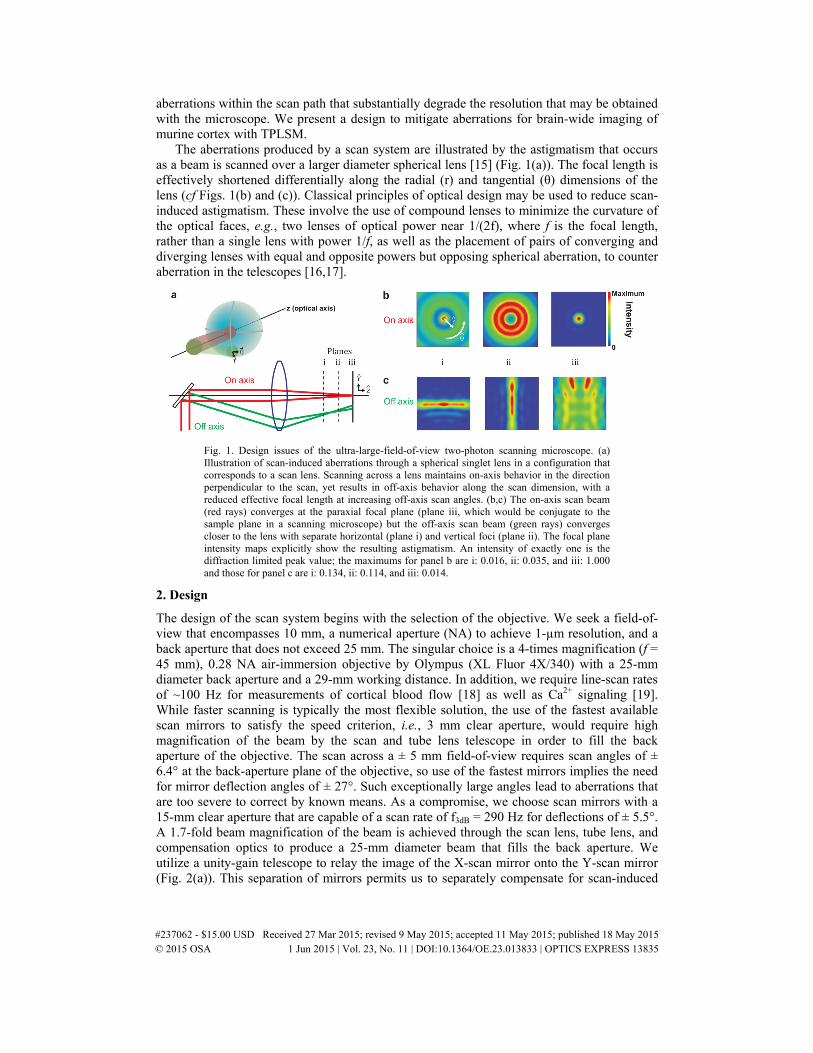
The aberrations produced by a scan system are illustrated by the astigmatism that occurs as a beam is scanned over a larger diameter spherical lens [15] (Fig. 1(a)). The focal length is effectively shortened differentially along the radial (r) and tangential (θ) dimensions of the lens (cf Figs. 1(b) and (c)). Classical principles of optical design may be used to reduce scan-induced astigmatism. These involve the use of compound lenses to minimize the curvature of the optical faces, e.g., two lenses of optical power near 1/(2f), where f is the focal length, rather than a single lens with power 1/f, as well as the placement of pairs of converging and diverging lenses with equal and opposite powers but opposing spherical aberration, to counter aberration in the telescopes [16,17].

Fig. 1. Design issues of the ultra-large-field-of-view two-photon scanning microscope. (a) Illustration of scan-induced aberrations through a spherical singlet lens in a configuration that corresponds to a scan lens. Scanning across a lens maintains on-axis behavior in the direction perpendicular to the scan, yet results in off-axis behavior along the scan dimension, with a reduced effective focal length at increasing off-axis scan angles. (b,c) The on-axis scan beam (red rays) converges at the paraxial focal plane (plane iii, which would be conjugate to the sample plane in a scanning microscope) but the off-axis scan beam (green rays) converges closer to the lens with separate horizontal (plane i) and vertical foci (plane ii). The focal plane intensity maps explicitly show the resulting astigmatism. An intensity of exactly one is the diffraction limited peak value; the maximums for panel b are i: 0.016, ii: 0.035, and iii: 1.000 and those for panel c are i: 0.134, ii: 0.114, and iii: 0.014.

2. Design

The design of the scan system begins with the selection of the objective. We seek a field-of-view that encompasses 10 mm, a numerical aperture (NA) to achieve 1-µm resolution, and a back aperture that does not exceed 25 mm. The singular choice is a 4-times magnification (f = 45 mm), 0.28 NA air-immersion objective by Olympus (XL Fluor 4X/340) with a 25-mm diameter back aperture and a 29-mm working distance. In addition, we require line-scan rates of ~100 Hz for measurements of cortical blood flow [18] as well as Ca2+ signaling [19]. While faster scanning is typically the most flexible solution, the use of the fastest available scan mirrors to satisfy the speed criterion, i.e., 3 mm clear aperture, would require high magnification of the beam by the scan and tube lens telescope in order to fill the back aperture of the objective. The scan across a ± 5 mm field-of-view requires scan angles of ± 6.4° at the back-aperture plane of the objective, so use of the fastest mirrors implies the need for mirror deflection angles of ± 27°. Such exceptionally large angles lead to aberrations that are too severe to correct by known means. As a compromise, we choose scan mirrors with a 15-mm clear aperture that are capable of a scan rate of f3dB = 290 Hz for deflections of ± 5.5°. A 1.7-fold beam magnification of the beam is achieved through the scan lens, tube lens, and compensation optics to produce a 25-mm diameter beam that fills the back aperture. We utilize a unity-gain telescope to relay the image of the X-scan mirror onto the Y-scan mirror (Fig. 2(a)). This separation of mirrors permits us to separately compensate for scan-induced


aberrations along the X- and Y-axes. Lastly, a matched converging/diverging lens-pair is inserted at the input to the scan system to compensate for the net on-axis spherical aberration (Fig. 2(a)).

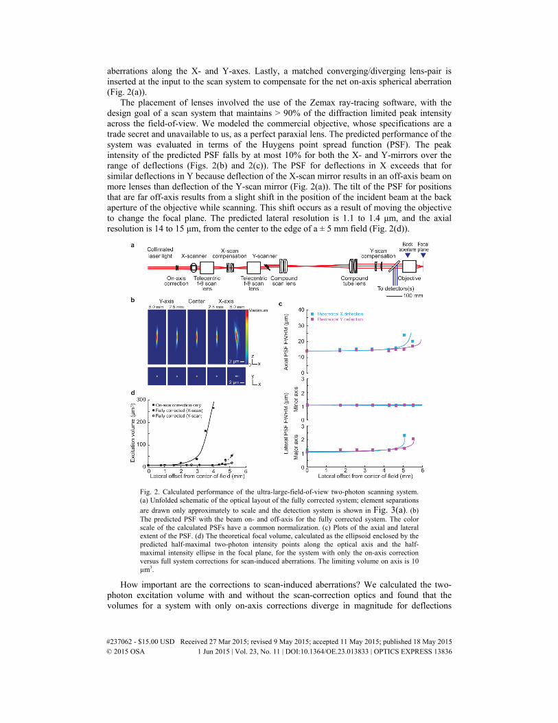
The placement of lenses involved the use of the Zemax ray-tracing software, with the design goal of a scan system that maintains > 90% of the diffraction limited peak intensity across the field-of-view. We modeled the commercial objective, whose specifications are a trade secret and unavailable to us, as a perfect paraxial lens. The predicted performance of the system was evaluated in terms of the Huygens point spread function (PSF). The peak intensity of the predicted PSF falls by at most 10% for both the X- and Y-mirrors over the range of deflections (Figs. 2(b) and 2(c)). The PSF for deflections in X exceeds that for similar deflections in Y because deflection of the X-scan mirror results in an off-axis beam on more lenses than deflection of the Y-scan mirror (Fig. 2(a)). The tilt of the PSF for positions that are far off-axis results from a slight shift in the position of the incident beam at the back aperture of the objective while scanning. This shift occurs as a result of moving the objective to change the focal plane. The predicted lateral resolution is 1.1 to 1.4 μm, and the axial resolution is 14 to 15 μm, from the center to the edge of a ± 5 mm field (Fig. 2(d)).

Fig. 2. Calculated performance of the ultra-large-field-of-view two-photon scanning system. (a) Unfolded schematic of the optical layout of the fully corrected system; element separations

are drawn only approximately to scale and the detection system is shown in Fig. 3(a). (b) The predicted PSF with the beam on- and off-axis for the fully corrected system. The color scale of the calculated PSFs have a common normalization. (c) Plots of the axial and lateral extent of the PSF. (d) The theoretical focal volume, calculated as the ellipsoid enclosed by the predicted half-maximal two-photon intensity points along the optical axis and the half-maximal intensity ellipse in the focal plane, for the system with only the on-axis correction versus full system corrections for scan-induced aberrations. The limiting volume on axis is 10 µm3.

How important are the corrections to scan-induced aberrations? We calculated the two-photon excitation volume with and without the scan-correction optics and found that the volumes for a system with only on-axis corrections diverge in magnitude for deflections


beyond 3 mm (Fig. 2(d)). The addition of scan correction optics leads to constant excitation volumes for deflections up to 4.5 mm that diverge only after 5.0 mm (Figs. 2(c) and 2(d)).

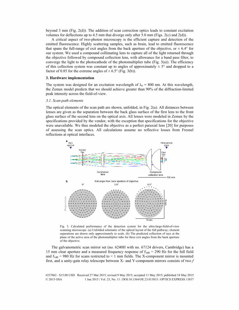
A critical aspect of two-photon microscopy is the efficient capture and detection of the emitted fluorescence. Highly scattering samples, such as brain, lead to emitted fluorescence that spans the full-range of exit angles from the back aperture of the objective, or ± 6.4° for our system. We used a compound collimating lens to capture all of the light returned through the objective followed by compound collection lens, with allowance for a band pass filter, to converge the light to the photocathode of the photomultiplier tube (Fig. 3(a)). The efficiency of this collection system was constant up to angles of approximately ± 5° and dropped to a factor of 0.85 for the extreme angles of ± 6.5° (Fig. 3(b)).

3. Hardware implementation

The system was designed for an excitation wavelength of λ0 = 800 nm. At this wavelength, the Zemax model predicts that we should achieve greater than 90% of the diffraction-limited peak intensity across the field-of-view.

3.1. Scan-path elements

The optical elements of the scan path are shown, unfolded, in Fig. 2(a). All distances between lenses are given as the separation between the back glass surface of the first lens to the front glass surface of the second lens on the optical axis. All lenses were modeled in Zemax by the specifications provided by the vendor, with the exception that specifications for the objective were unavailable. We thus modeled the objective as a perfect paraxial lens [20] for purposes of assessing the scan optics. All calculations assume no reflective losses from Fresnel reflections at optical interfaces.

Fig. 3. Calculated performance of the detection system for the ultra-large-field-of-view scanning microscope. (a) Unfolded schematic of the optical layout of the full pathway; element separations are drawn only approximately to scale. (b) The predicted collection of rays at the plane of the active area of the photomultiplier tube for three exit angles from the back aperture of the objective.

The galvanometric scan mirror set (no. 6240H with no. 67124 drivers, Cambridge) has a 15 mm clear aperture and a measured frequency response of f3dB = 290 Hz for the full field and f3dB = 980 Hz for scans restricted to < 1 mm fields. The X-component mirror is mounted first, and a unity-gain relay telescope between X- and Y-component mirrors consists of two f


= 100 mm f-θ scan lenses (632-nm design wavelength; no. 64-426, Edmund Optical) in opposing orientations with threads towards the scan mirrors. We place four singlet lenses, arranged as oppositely oriented symmetric pairs between the f-θ scan lenses, to correct for astigmatism. Two f = 250 mm positive plano-convex lenses (2” diameter, BK7 material; no. LA1301, Thorlabs) are placed 80.5 mm from each f-θ scan lens with the planar face towards the nearest scan lens. Two f = −250-mm biconcave lenses (2” diameter, silica material; no. 018-0690. Optosigma) are placed 5 mm from each plano-convex lens, and 16.1 mm from each other. The f-θ scan lenses are mounted 32 mm and 31 mm from the X- and Y- component mirrors, respectively.

A telescope that consists of a compound scan lens and compound tube lens relays the image of the galvanometric scan mirrors to the back aperture of the objective. The Y-component mirror is followed by the compound scan lens, which consists of an identical pair of cemented f = 310 mm achromatic doublets (3” diameter; no. 322278000, Qioptiq) that are separated by an air gap of 1 mm. Both doublets are oriented so that the surface of least curvature faces the scan mirrors, and are placed 143.8 mm from the Y-scan mirror. The compound tube lens is placed 387.2 mm from the compound scan lens and consists of a f = 310 mm cemented achromatic doublet (3” diameter; no. 322278000, Qioptiq) and a f = 1159 mm doublet (3” diameter; no. 322242000, Qioptiq) that are separated by an air gap of 1 mm. Both doublets are oriented so that the surface of greatest curvature faces towards the compound scan lens. As a practical issue, a folding mirror is inserted approximately 100 mm upstream of first element of the tube lens to redirect the beam towards the table.

We compensated for scan-induced aberrations from the tube lens and scan lens with an additional lens pair situated 114 mm downstream from the compound tube lens. The pair consists of a plano-concave lens, with f = −150-mm (2” diameter, BK7 material, no. LC1611, Thorlabs) and a f = 175-mm bi-convex lens (2” diameter, BK7 material, no. LA1399, Thorlabs) separated by 28 mm.

3.2. Table elements

Our oscillator is a Mira HP (Coherent Inc.) that is pumped by an 18 W Verdi (Coherent). The system produces a 1-mm diameter beam with greater than 2 W of average laser power at a center wavelength of 800 nm with 100-fs pulses at a repetition rate of 80 MHz. We use two sequential telescopes to expand the beam to fill the 15-mm clear aperture scan mirrors. The first telescope consists of a f = 150 mm achromatic doublet (1” diameter; AC254-150-B, Thorlabs) and a f = 750 mm achromatic doublet (2” diameter; AC508-750, Thorlabs). The second telescope consists of a f = 250-mm achromatic doublet (1” diameter; AC254-250-B, Thorlabs) and a f = 1000-mm achromatic doublet (2” diameter; AC508-1000, Thorlabs).

The first telescope pair after the oscillator has a lens separation of 890 mm and the second telescope pair has a lens separation of 984 mm. The second telescope pair is placed 290 mm from the first telescope pair. The compensation pair, discussed below, is placed 200 mm from the second telescope pair and 530 mm from the X-scan mirror through a periscope to raise the beam to the horizontal plane of the scan mirrors. The telescope pairs separation deviate from typical sum-of-focal length separations to offset the initial beam divergence of the laser output and the net convergence of the compensation pair to produce an expanded, collimated beam as input to the X-scan mirror.

The final optical element prior to the first scan mirror is a pair of singlet lenses that are separated by a 2.5 mm air gap and which serves to compensate for the net on-axis spherical aberration through the remaining lenses of the scanning system. The first lens is a f = −100 mm planoconcave lens (1” diameter, BK7 material; LC1254, Thorlabs) oriented so that the planar surface faces the laser source. The second lens is a f = 100 mm bi-convex lens (1” diameter, silica material; LB4941, Thorlabs).


3.3. Detection pathway

The optical elements of the detection path are shown, unfolded, in Fig. 3(a). The collection pathway utilizes 2” and 3” diameter optics to maximize the collection of the emitted fluorescent light across the entire 10-mm field of the 4-times magnification objective used in our system. As with the scan system, distances between lenses are given as the separation between back surface of the first lens to the front surface of the second lens on the optical axis. The collection system consists of a 2” clear aperture dichroic mirror (FF775-Di01-49x78, Semrock) positioned 75 mm from the back aperture plane of the objective. This is followed by a + 200-mm focal length achromatic doublet (AC508-200, Thorlabs) placed 110 mm from the back aperture plane of the objective. This is next followed by a 150-mm gap and a 3” diameter, 99.65-mm focal length singlet lens (LA1238, Thorlabs). This lens is separated by a 1-mm gap from a 3” diameter, 60-mm focal length aspheric lens (ACL7560, Thorlabs). Lastly, this is followed by a 7.6 mm gap to two 1” diameter, 3-mm thick filters (BG39, Andover). The second filter is located 1 mm from the final collection lens; a ½” diameter, 25-mm focal length singlet lens is mounted 3 mm in front of the active area of a GaAsP PMT (H10770B-40, Hammamatsu).

4. System validation

A shear plate interferometer was used to optimize collimation at the location of the back aperture of the microscope objective and determine aberrations on optical beams. Shearing interferometry operates by interfering an optical wave-front with a laterally shifted and angularly tilted replica of itself; the resultant fringe pattern contains information about the wave-front [21]. In practice, this is accomplished with a slightly wedged thick glass plate [22].

In our setup, all optics were initially aligned in position according to a Zemax model of the optical set-up. With the objective removed, a shear plate (no. SI500P, Thorlabs) was inserted in the beam and its reflection was monitored with a CCD camera. Interference fringes were readily observed and indicated if the beam was collimated. In brief, collimation is indicated by flat horizontal fringes, divergence is indicated by fringes tilting clockwise, convergence is indicated by fringes tilting counterclockwise, and spherical aberration is indicated by “S-shaped” fringes. Shifts in the alignment of optical elements were made to obtain the flattest horizontal fringes possible over the full range of scan angles of the system. The resultant measured divergences were on the order of < 1 milliradian across the range of scan angles (Fig. 4(a)) and had negligible spherical or higher order aberration. Note that as a general tool, the shearing interferogram also contains information about coma, astigmatism, and higher order Zernike polynomials [23].

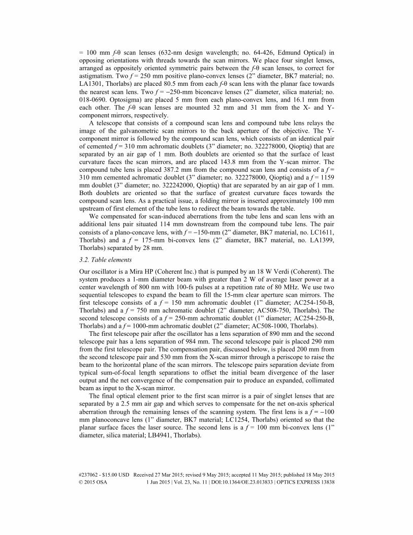
Fig. 4. Beam characteristic of the ultra-large-field-of-view two-photon scanning microscope. (a) Experimental verification of beam collimation across the full range of scan angles utilizing an interferometric shear plate. The rotation of the interference fringes at large scan angles, found from the slopes of the fringes (yellow lines) for the center and x = 4.3 mm scan positions, is consistent with a residual beam divergence of less than 1 mrad. (b) The envelope of the interferometric autocorrelation of the laser pulses evaluated through the full optical path of the microscope at the focus of the objective. The calculated fit (red) to the envelope of the experimental data (blue) is consistent with an initial pulse width of 110 fs (FWHM) that is chirped to a final width of 400 fs.


In order to measure the pulse duration at the sample, an interferometric autocorrelation was performed by utilizing a Michelson delay line prior to the scanning setup. Two-photon fluorescence in a bath of fluorescein was recorded as a function of delay, the autocorrelation trace was recorded, and the measured signal was modeled using a Matlab fitting algorithm. The totality of dispersion through all lenses increased the width of laser pulses from a native 110 fs to 400 fs (Fig. 4(b)). No compensation to recompress the pulse was used.

We assessed the off-axis throughput of the objective in terms of the efficiency of two-photon excited fluorescence from a uniform bath of fluorescein. There is a 47% decrease in fluorescent intensity for scan mirror deflections of ± 5 mm (Figs. 5(a) and 5(b)). This exceeds the 10% decrease expected from residual aberration in the scan system design (Fig. 2(c)). To test if this decrement results from the non-ideal nature of the objective, we parked the scan mirrors for on-axis illumination and tilted the objective about an axis in the plane of the back aperture (Fig. 5(b)). These measurements mimics the performance of the objective at nonzero scan angles yet eliminates scan-dependent variations to the beam profile and to the collection path. Comparison of the intensity profiles obtained by scanning of the galvanometric mirror (red and blue lines, Fig. 5(b)) with that obtained by tilting of the objective (green line, Fig. 5(b)) shows that our design is limited by the performance of the objective.

We determined the resolution of the realized system by measurements of the PSF (Fig. 5(c)). To evaluate image quality, we embed sub-resolution, 0.5-µm fluorescent beads in 1% (w/v) agarose (no. A9793, Sigma) and imaged them through a number 0 cover glass. Image stacks were acquired across a 40-µm lateral field through a depth of 400 µm with a lateral sampling of 0.08 µm per pixel and an axial sampling of 0.3 µm per frame to produce a 3-dimensional intensity distribution of the TPLSM signal from the bead, I(r, z). The reported lateral resolutions are the full width at half-maximal (FWHM) intensity along either the x- or y-axis in the plane of highest peak intensity. The reported axial resolution is the FWHM intensity along the central axial line through the bead in the longitudinal slice of highest intensity of the rotated image stack. Focal volumes are reported as the volume of the ellipsoid enclose by axial and lateral widths.

We performed a small amplitude scan with the galvanometric mirrors at varying offset angles within the field-of-view. The observed axial resolution is 16 μm at the center and degrades to 33 μm at the edge of the field (Fig. 5(d)). The lateral resolution is 1.2 μm at the center and degrades to a 1.5 x 2.0 μm ellipse at the edge of the field. Second, we performed a small amplitude scan with the mirrors centered but with the objective tilted relative to the on-axis beam. The PSFs obtained by tilting the objective (green symbols, Figs. 5(d) and 5(e)) are comparable to those found by scanning (red and blue symbols, Figs. 5(d) and 5(e)). Thus, while the final resolution of our microscope is limited by the performance of the objective, this resolution is achieved only with compensation for scan-induced aberrations.


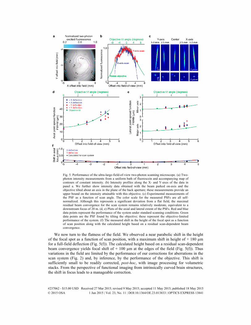
Fig. 5. Performance of the ultra-large-field-of-view two-photon scanning microscope. (a) Two-photon intensity measurements from a uniform bath of fluorescein and accompanying map of contours of constant intensity. (b) Intensity profiles along the X- and Y-axes of the data in panel a. We further show intensity data obtained with the beam parked on-axis and the objective tilted about an axis in the plane of the back aperture; these measurements provide an upper bound on the intensity attainable with this objective. (c) Experimental measurements of the PSF as a function of scan angle. The color scale for the measured PSFs are all self-normalized. Although this represents a significant deviation from a flat field, the maximal residual beam convergence for the scan system remains relatively moderate, equivalent to a downstream focus of 20 m. (d, e) Plots of the axial and lateral extent of the PSFs. Red and blue data points represent the performance of the system under standard scanning conditions. Green data points are the PSF found by tilting the objective; these represent the objective-limited performance of the system. (f) The measured shift in the height of the focal spot as a function of scan position along with the calculated height based on a residual scan-dependent beam convergence.

We now turn to the flatness of the field. We observed a near parabolic shift in the height of the focal spot as a function of scan position, with a maximum shift in height of + 180 µm for a full-field deflection (Fig. 5(f)). The calculated height based on a residual scan-dependent beam convergence yields focal shift of + 100 µm at the edges of the field (Fig. 5(f)). Thus variations in the field are limited by the performance of our corrections for aberrations in the scan system (Fig. 2) and, by inference, by the performance of the objective. This shift is sufficiently small to be readily corrected, post-hoc, with image processing for volumetric stacks. From the perspective of functional imaging from intrinsically curved brain structures, the shift in focus leads to a manageable correction.


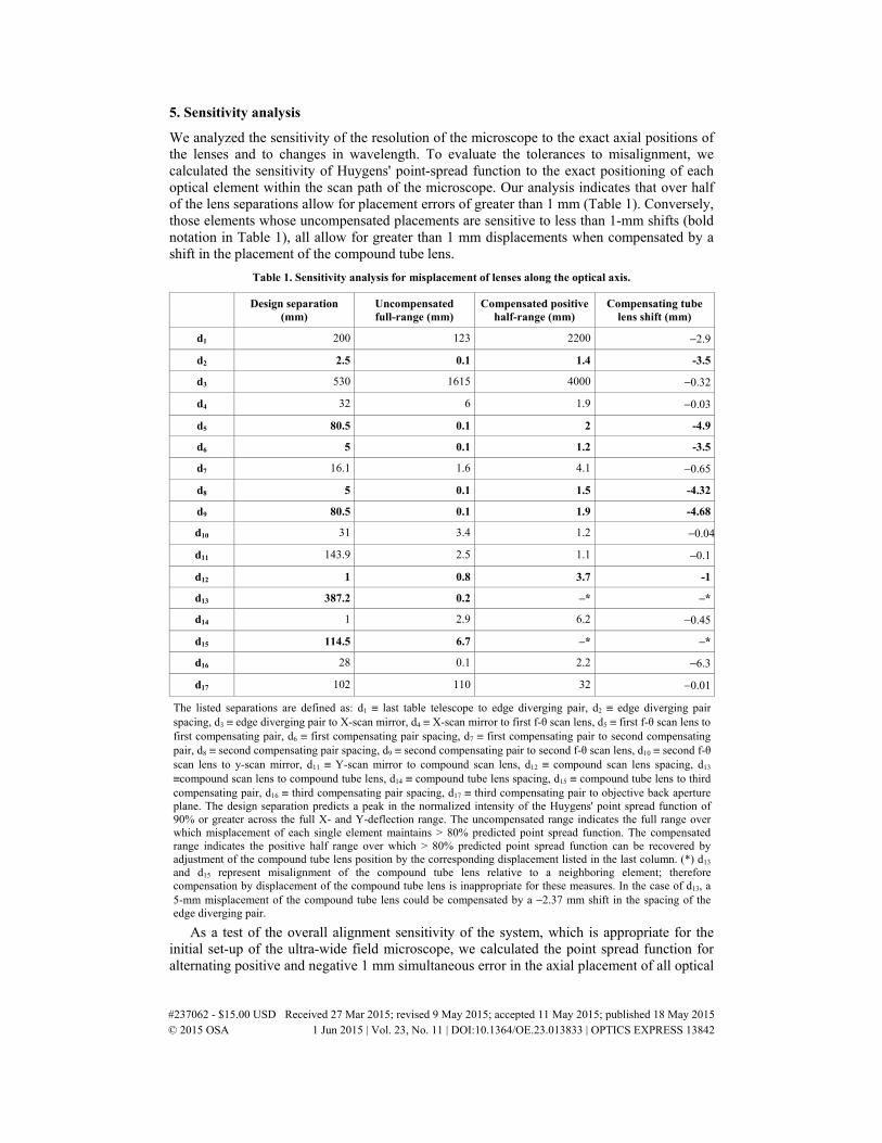
5. Sensitivity analysis

We analyzed the sensitivity of the resolution of the microscope to the exact axial positions of the lenses and to changes in wavelength. To evaluate the tolerances to misalignment, we calculated the sensitivity of Huygens' point-spread function to the exact positioning of each optical element within the scan path of the microscope. Our analysis indicates that over half of the lens separations allow for placement errors of greater than 1 mm (Table 1). Conversely, those elements whose uncompensated placements are sensitive to less than 1-mm shifts (bold notation in Table 1), all allow for greater than 1 mm displacements when compensated by a shift in the placement of the compound tube lens.

Table 1. Sensitivity analysis for misplacement of lenses along the optical axis.

Design separation (mm)

Uncompensated full-range (mm)

Compensated positive half-range (mm)

Compensating tube lens shift (mm)

d1 200 123 2200 −2.9

d2 2.5 0.1 1.4 -3.5

d3 530 1615 4000 −0.32

d4 32 6 1.9 −0.03

d5 80.5 0.1 2 -4.9

d6 5 0.1 1.2 -3.5

d7 16.1 1.6 4.1 −0.65

d8 5 0.1 1.5 -4.32

d9 80.5 0.1 1.9 -4.68

d10 31 3.4 1.2 −0.04

d11 143.9 2.5 1.1 −0.1

d12 1 0.8 3.7 -1

d13 387.2 0.2 –* –*

d14 1 2.9 6.2 −0.45

d15 114.5 6.7 –* –*

d16 28 0.1 2.2 −6.3

d17 102 110 32 −0.01

The listed separations are defined as: d1 ≡ last table telescope to edge diverging pair, d2 ≡ edge diverging pair spacing, d3 ≡ edge diverging pair to X-scan mirror, d4 ≡ X-scan mirror to first f-θ scan lens, d5 ≡ first f-θ scan lens to first compensating pair, d6 ≡ first compensating pair spacing, d7 ≡ first compensating pair to second compensating pair, d8 ≡ second compensating pair spacing, d9 ≡ second compensating pair to second f-θ scan lens, d10 ≡ second f-θ scan lens to y-scan mirror, d11 ≡ Y-scan mirror to compound scan lens, d12 ≡ compound scan lens spacing, d13 ≡compound scan lens to compound tube lens, d14 ≡ compound tube lens spacing, d15 ≡ compound tube lens to third compensating pair, d16 ≡ third compensating pair spacing, d17 ≡ third compensating pair to objective back aperture plane. The design separation predicts a peak in the normalized intensity of the Huygens' point spread function of 90% or greater across the full X- and Y-deflection range. The uncompensated range indicates the full range over which misplacement of each single element maintains > 80% predicted point spread function. The compensated range indicates the positive half range over which > 80% predicted point spread function can be recovered by adjustment of the compound tube lens position by the corresponding displacement listed in the last column. (*) d13 and d15 represent misalignment of the compound tube lens relative to a neighboring element; therefore compensation by displacement of the compound tube lens is inappropriate for these measures. In the case of d13, a 5-mm misplacement of the compound tube lens could be compensated by a −2.37 mm shift in the spacing of the edge diverging pair.

As a test of the overall alignment sensitivity of the system, which is appropriate for the initial set-up of the ultra-wide field microscope, we calculated the point spread function for alternating positive and negative 1 mm simultaneous error in the axial placement of all optical


elements. We found that the predicted performance remained above 79% of the diffraction limit, compared to 90% of the diffraction limit for the unaltered system, with an overall focal shift of −63 µm. For completeness, Table 1 includes the positive half range for which misplacement of a single element is compensated by displacement of the compound tube lens to 80% or better of the predicted performance.

We turn to the performance at commonly used excitation wavelengths other than λ0 = 800 nm [24]. The Zemax model predicts that the diffraction limited peak intensity is maintained to within 6% of the value at 800 nm by judicious shifts in the position of lenses. The majority of the shifts are confined to the arm between the scan mirrors (Fig. 2(a)), for which the separation of the f-θ scan lens from the X-scan mirror is changed from 32.0 mm (800 nm) to 31.5 mm (750 nm), 33.0 mm (1300 nm), or 34.5 mm (1700 nm), the separation of the other f-θ scan lens from the Y-scan mirror is changed from 31.5 mm (800 nm) to 30.5 mm (750 nm), 31.0 mm (1000 nm), 32.0 mm (1300 nm), or 33.5 mm (1700 nm), the separation between each f-θ scan lens and its nearest plano-convex lenses is changed from 80.5 mm (800 nm) to 83.0 mm (750 nm), 71.5 mm (1000 nm), 62.0 mm (1300 nm), or 49.5 mm (1700nm), the separation between each plano-convex lens to the neighboring biconcave lens is changed from 5.00 mm (800 nm) to 2.38 mm (750 nm), 13.87 mm (1000 nm), 23.53 mm (1300 nm), or 34.2 mm (1700 nm), and, lastly, the separation between the pair of biconcave lenses is changed from 16.1 mm (800 nm) to 11.0 mm (1300 nm), or 9.0 mm (1700 nm). The arm between the Y-scan mirror and the objective requires a change only at long wavelengths, i.e., the separation of the compound scan lens to the tube lens is increased from 387.2 mm (800 nm) to 398 mm (1300 nm) or 408 mm (1700 nm).

6. Applications

We use the ultra-large field-of-view microscope to address our motivating issue of spatial correlations in vasomotion in awake, head-fixed mice. We simultaneously monitored the diameter of individual pial arterioles in separate hemispheres (Figs. 6(a) and 6(b)), as well as pial venules as controls, at an excitation wavelength of λ = 800 nm. Post-processing of the images consisted only of scaling the brightness and contrast. Spectral analysis confirms that the variation in the arteriole diameters exhibits significant power and coherence in the nominal 0.1 to 0.5 Hz band of vasomotion (red and green curves in Fig. 6(c)). Such vasomotion was more than 3-times less in amplitude in pial venules (blue curve in Fig. 6(c)), consistent with previous reports [6], and roughly two orders of magnitude above the system noise level (gray curve in Fig. 6(c)).

Further analysis of the above functional data indicates synchrony between the low-frequency vasomotion in arterioles that lie in these two widely separated regions of the cortical mantle, as seen in the cross-correlation (Fig. 6(d)). This synchrony is statistically significant in the frequency band of vasomotion (Fig. 6(e)). The distance between the vessels in the different hemispheres far exceeds the ~2 mm electrotonic length for coupling among vascular endothelial cells [25], which serves as the conduction pathway for vasomotion [26]. The observed correlation is consistent with a neuronal mechanism for transhemispheric coordination of vascular dynamics, as is assumed for resting state fMRI [5].

The cross-hemispheric correlation of pial vessels (Fig. 6) required only modest depth penetration. A scan across an entire window above one hemisphere (Fig. 6a) shows that microvessels are well resolved within the field, as seen in a maximum projection of images from the pial surface to 210 µm below the pial (Fig. 7(a)) and in individual planar scans taken at the center of the field (Fig. 7(b)). Further, the flow of individual red blood cells (RBCs) within a microvessel could be tracked, in addition to the diameter, with an curvilinear path in arbitrary line scan mode [27] (Fig. 7(c)). These data demonstrate the capability of the ultra-large field-of-view microscope for quantitative imaging.


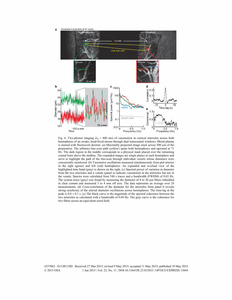
Fig. 6. Two-photon imaging (λ0 = 800 nm) of vasomotion in cortical arterioles across both hemispheres of an awake, head-fixed mouse through dual transcranial windows. Blood plasma is stained with fluorescein dextran. (a) Maximally projected image stack across 500 µm of the preparation. The arbitrary-line-scan path (yellow) spans both hemispheres and operated at 71 Hz. The dark region in the middle corresponds to a physical mask placed over the remaining cranial bone above the midline. The expanded images are single planes in each hemisphere and serve to highlight the path of the line-scan through individual vessels whose diameters were concurrently monitored. (b) Vasomotor oscillations measured simultaneously from pial arteries in the right (green) and left (red) hemispheres. An expanded and overlaid view of the highlighted time band (gray) is shown on the right. (c) Spectral power of variation in diameter from the two arterioles and a venule (panel a) indicate vasomotion in the arterioles but not in the venule. Spectra were calculated from 540 s traces and a bandwidth (FWHM) of 0.03 Hz. The system noise (gray) was found by measuring the diameter of 8 to 20 µm fibers imbedded in clear cement and measured 3 to 4 mm off axis. The data represents an average over 24 measurements. (d) Cross-correlation of the diameter for the arterioles from panel b reveals strong synchrony of the arterial diameter oscillations across hemispheres. The time-lag at the peak is 0.0 ± 0.1 s. (e) The black curve is the magnitude of the spectral coherence between the two arterioles as calculated with a bandwidth of 0.04 Hz. The gray curve is the coherence for two fibers across an equivalent sized field.


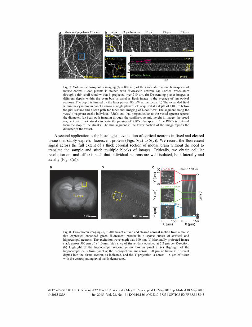
Fig. 7. Volumetric two-photon imaging (λ0 = 800 nm) of the vasculature in one hemisphere of mouse cortex. Blood plasma is stained with fluorescein dextran. (a) Cortical vasculature through a thin skull window that is projected over 210 µm. (b) Descending planar images at different depths within the cyan box in panel a. Each image is the average of ten optical sections. The depth is limited by the laser power, 80 mW at the focus. (c) The expanded field within the cyan box in panel a shows a single planar field acquired at a depth of 110 µm below the pial surface and a scan path for functional imaging of blood flow. The segment along the vessel (magenta) tracks individual RBCs and that perpendicular to the vessel (green) reports the diameter. (d) Scan path imaging through the capillary. At mid-height in image, the broad segment with dark streaks indicate the passing of RBCs; the speed of the RBCs is inferred from the slop of the streaks. The thin segment in the lower portion of the image reports the diameter of the vessel.

A second application is the histological evaluation of cortical neurons in fixed and cleared tissue that stably express fluorescent protein (Figs. 8(a) to 8(c)). We record the fluorescent signal across the full extent of a thick coronal section of mouse brain without the need to translate the sample and stitch multiple blocks of images. Critically, we obtain cellular resolution on- and off-axis such that individual neurons are well isolated, both laterally and axially (Fig. 8(c)).

Fig. 8. Two-photon imaging (λ0 = 900 nm) of a fixed and cleared coronal section from a mouse that expressed enhanced green fluorescent protein in a sparse subset of cortical and hippocampal neurons. The excitation wavelength was 900 nm. (a) Maximally projected image stack across 500 µm of a 1.0-mm thick slice of tissue; data obtained at 2.2 µm per Z-section. (b) Highlight of the hippocampal region; yellow box in panel a. (c) Highlight of the hippocampal cells from panel a; the Z-projections are across ~60 µm of tissue at different depths into the tissue section, as indicated, and the Y-projection is across ~15 µm of tissue with the corresponding axial bands demarcated.


7. Discussion

We have demonstrated the design and application a ultra-large field-of-view two-photon microscope that maintains sufficient lateral resolution to resolve cells and vessels across a 10-mm field-of-view. The primary strength of this approach is the ability to simultaneous image brain activity in tissue regions separated by distances that can vary continuously up to distances of many millimeters. We used the system as a tool for the analysis of mesoscopic neurovascular dynamics across cortical hemispheres. Further, we showed that whole tissue may be imaged without the need to stitch together smaller fields of view. This circumvents the need to correct for differential distortions at the edges of the tiled fields.

A weakness of our initial realization of the microscope is the reduced spatial resolution that results from the use of a 4X, 0.28 NA objective as compared to the higher numerical aperture objectives, NA ~0.8 to 1.0, objectives typically used for TPLSM, included TPLSM with a 1.4-mm field [28]. Yet our lower resolution is accompanied by a two- to three-order-of-magnitude large field-of-view. A readily available improvement to our initial realization is the addition of anti-reflection coatings to our uncoated lenses, which currently results in significant loss of transmitted laser power. Nevertheless, the principles of our design yields a large diameter scanned beam that is free of astigmatism across a wide range of scan angles. This beam is suitable for any infinity-conjugated objective. Thus we can immediately take advantage of future improvements in the design of low-magnification, high-numerical aperture objectives.

8. Sample preparation

8.1 Mouse surgery

We used 3 male adult C57/Bl6 mice, 8 to 12 weeks old that were obtained from Jackson Lab. A pair of thin-skull transcranial windows, each over an area of 2.5 mm by 2.5 mm that spanned the parietal region of each hemispheres, were prepared by an extension of previous described procedures [12, 29]. A drop of cyanoacrylate glue (no. 401 Loctite) was put on the thinned region and precut #0 cover glasses capped the cement. A crown-like custom made metal implant was glued onto the skull for head fixation, and the remaining bone, the implant, and the region over the central sinus was reinforced with cyanoacrylate glue and dental cement to increase stability. All surgical procedures were approved by the Institutional Animal Care and Use Committees of University of California, San Diego.

8.2. In vivo imaging

The mouse was permitted to recover for three days, then habituated to head-fixation over a period of four days until a period of one hour continuous recording was readily achieved. On the day of experimentation, the mouse was head-fixed and briefly anesthetized to label the lumen of blood vessels with a 50 µL retro-orbital injection of 5% (w/v) fluorescein-labeled dextran (2 MDa, Sigma). The awake mouse was then positioned on the microscope. Large-field maps of the pial vessels at high resolution were obtained at low frame rate (0.32 Hz, 2,000 by 500 pixels). Dynamic measurements of vessel diameters across hemispheres were performed with an arbitrary scanning path that passes through all vessels of interest with a line frequency of 71 Hz. Arbitrary scans through capillaries in a single hemisphere were performed with a line frequency of 484 Hz. Dynamical measurements were analyzed with code written in Matlab using the Chronux open-source software package (www.chronux.org). The spectral power was computed with a time-bandwidth product of 16 and the coherence was computed with a time-bandwidth product of 27.

8.3 Fixed tissue preparation

Two Thy-1-GFP-S mice (CBA-Tg(Thy1-EGFP)SJrs/NdivJ; number: 011070, Jackson Laboratory) were used for fixed tissue imaging of sparsely distributed neurons in the


neocortex that expressed green fluorescence protein. Tissue was prepared as described previously and cleared by graded immersion that led to a 60% (w/v) solution of sucrose over a course of two days [30]. After clearing, 1-mm-thick coronal slices were mounted in a gel of 60% (w/v) sucrose and 1% (w/v) agarose (no. A9793, Sigma) in a 35-mm petri dish (no. BD351008, Falcon) and covered with a number 1 glass coverslip.

Acknowledgments

We thank Jonathan Driscoll for assistance with the software and Jürgen Sawinski, Jeffrey Squier and Donald Welch for discussions. This work was supported by grants from the Center for Brain Activity Mapping at UCSD (2013-018) and the National Institutes of Health (EB003832, MH108503, and OD006831).


Ultra-large field-of-view two-photon microscopy

Documents

Transcript of Ultra-large field-of-view two-photon microscopy