04/02/2010

CENTRE FOR COMPARATIVE ECONOMICS

UCL SSEESCentre for Comparative Economics

“Mass Privatisation and the Post-Communist Mortality Crisis”: Is There Really a

Relationship?

John S. Earlea and Scott Gehlbachb

a Upjohn Institute for Employment Research and Central European University, email: earle@upjohn.orgb University of Wisconsin-Madison, e-mail: gehlbach@polisci.wisc.edu

Economics Working Paper No.105

February 2010

Centre for Comparative EconomicsUCL School of Slavonic and East European Studies

Gower Street, London, WC1E 6BTTel: +44 (0)20 7679 8519Fax: +44 (0)20 7679 8777

Email: cce@ssees.ucl.ac.uk

“Mass Privatisation and the Post-Communist MortalityCrisis”: Is There Really a Relationship?∗

John S. EarleUpjohn Institute for Employment Research

and Central European UniversityEmail: earle@upjohn.org

Scott GehlbachUniversity of Wisconsin–MadisonE-mail: gehlbach@polisci.wisc.edu

January 2010

A summary of this paper is available as John S. Earle and Scott Gehlbach, “DidMass Privatisation Really Increase Post-Communist Mortality?” The Lancet,375(9712):372, available at http://www.thelancet.com/journals/lancet/article/

PIIS0140-6736(10)60159-6/fulltext.

∗Thanks to Jing Cai and Attila Osztotics for assistance with the cross-country analysis, to Galina Be-lokurova and Emily Sellars for help with the Russia analysis, to Michael Spagat for comments, and toLarry King for sharing the country-level data used in Stuckler, King and McKee (2009). Useful feedback wasreceived from seminar and conference participants at Harvard University, Hitotsubashi University, UW Madi-son, the Ronald Coase Institute Workshop on Institutional Analysis in Bratislava, the 2009 annual meetingof the International Society for New Institutional Economics, the 2009 annual meeting of the Midwest Po-litical Science Association, and the 2009 annual meeting of the American Association for the Advancementof Slavic Studies.

1

Abstract

We reexamine the recent, well-publicized claim that “rapid mass privatisation [of state-owned enterprises]. . . was a crucial determinant of differences in adult mortality trendsin post-communist countries” (Stuckler, King and McKee, 2009). Our analysis showsthat the estimated correlation of privatization and mortality in country-level data isnot robust to recomputing the mass-privatization measure, to assuming a short lag foreconomic policies to affect mortality, and to controlling for country-specific mortalitytrends. Further, in an analysis of the determinants of mortality in Russian regions, wefind no evidence that privatization increased mortality during the early 1990s. Finally,we reanalyze the relationship between privatization and unemployment in postcom-munist countries, showing that there is little support for the proposed mechanism bywhich privatization might have increased mortality.

1 Introduction

In the early 1990s, the postcommunist countries of Eastern Europe and the former SovietUnion initiated changes that would fundamentally transform their political and economicinstitutions. Coincident with these changes, many countries in the region experienced adramatic increase in mortality, especially among working-age males. Various studies haveinvestigated this mortality spike, but debate continues on the underlying causal mechanisms.1

In a recent, well-publicized contribution to this literature, David Stuckler, Lawrence King,and Martin McKee (henceforth SKM) argue in The Lancet that “rapid mass privatisation [ofstate-owned enterprises]. . . was a crucial determinant of differences in adult mortality trendsin post-communist countries” (Stuckler, King and McKee, 2009, p. 1).2 The evidence offeredin support of this claim consists of country-level regressions of the adult male mortality rateon measures of enterprise privatization. The authors’ primary interpretation is that rapidprivatization increased unemployment and consequently illness, for which they offer supportfrom country-level analysis of unemployment. The estimated effects of mass privatizationon both mortality and unemployment are reported to be positive and statistically significantonly in the former Soviet Union; no evident effects are reported among Central and EastEuropean countries.

The publication of SKM’s study has reignited debate over the effects of economic reform. Theprovocative tone of the Economist leader on the topic—“Mass Murder and the Market”—reflects the stakes involved: should reformers be held responsible for millions of prematuredeaths?3 Jeffrey Sachs, an architect of “shock therapy” in postcommunist countries, sug-gests that the study is a “confused polemic that will not withstand serious epidemiologi-cal scrutiny.”4 On the other side, Joseph Stiglitz argues that “[The] Lancet is right thatPoland was an example of more gradual policies”—the study credits gradualism with re-duced mortality—and reasserts his view that “‘shock therapy’ was a disastrous economicpolicy.”5

Did mass privatization increase mortality in postcommunist countries? In this paper, we re-examine this relationship. We find that the estimated effect of privatization in cross-countrydata is not robust to recomputing the mass privatization measure using original source data,to assuming short lags between economic policies and changes in mortality rates, and tocontrolling for country-specific mortality trends. We also examine the relationship betweenprivatization and mortality across Russian regions, finding no evidence that privatizationwas responsible for the large increase in Russian mortality during the early 1990s. Finally,we reanalyze the relationship between privatization and unemployment. Counter to the

1Cornia and Paniccia (2000), Shkolnikov et al. (2004), and Stillman (2006) provide extensive reviews.Recent studies that investigate the impact of particular policies and societal characteristics include Brainerdand Cutler (2005), Bobak et al. (2007), Treisman (2008), and Denisova (2009).

2All page numbers refer to the online version of SKM.3“Mass Murder and the Market,” Economist, January 22, 2009.4“‘Shock Therapy’ Had No Adverse Effect on Life Expectancy in Eastern Europe,” Jeffrey D. Sachs,

letter to the Financial Times published January 19, 2009.5“Stiglitz on Death and Privatization in the Eastern Bloc,” New York Times Economix blog, January

16, 2009.

1

claims of SKM, there is no robust evidence that privatization increased unemployment inpostcommunist countries.

2 Cross-Country Analysis

The results in SKM raise a number of questions concerning sample, data, definitions, andmethods: Are the measures of privatization appropriate? Are any effects of privatizationon mortality instantaneous? Are there no pre-existing trends in the data? How much canone conclude from a sample of only 15 countries (the FSU sample), and is country theright level of analysis? More generally, is the privatization coefficient identified, statisticallydistinguishable from other factors that may have affected mortality? And what is the causalmechanism that might link mortality with privatization? We address these questions througha series of related research designs.

We begin by reexamining the cross-country correlation between mortality and privatization.The evidence put forward by SKM is based on an unbalanced panel of 24 countries observedannually from 1989 to 2002, but a positive impact of privatization on mortality is estimatedonly for the 15 former republics of the Soviet Union (FSU), not for the 9 countries of Centraland Eastern Europe (CEE). We therefore focus attention on the former group; results forCEE are available in Table A1 in the Appendix.

We first perform pure replications using the SKM regression specifications. The dependentvariable in SKM and our replications is the natural log of the age-standardized mortalityrate for males aged 15–59. SKM use two alternative measures of privatization in differentspecifications: a “mass privatization” indicator and the “average EBRD privatization index,”the latter the average of two widely used measures of progress in privatization published inthe annual Transition Report of the European Bank for Reconstruction and Development(e.g., EBRD, 2007). We discuss both measures further below. In all specifications, SKMinclude country fixed effects, and they control for various time-varying country characteris-tics: log income, price liberalization, foreign exchange/trade liberalization, democracy, war,population dependency, urbanization, and higher education.

Columns (1) and (2) of the first row of estimates in Table 1 present these replications. Theresults are very similar to those published in SKM. There is a positive estimated impact ofprivatization using both measures in the FSU sample. As in SKM, the estimated impact iszero in CEE (as shown in Table A1). Results for the control variables are not reported inSKM, so we suppress them here as well (they are available on request).

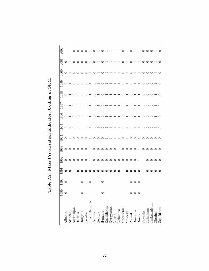
We next use original source data to reexamine the SKM privatization variables. (Withthe exception of these variables, we continue to use the SKM data in all specifications.)Beginning with the mass privatization indicator, the SKM definition is “a programme thattransferred the ownership of at least 25% of large state-owned enterprises to the privatesector in 2 years. . . 0 before mass privatisation, 1 thereafter,” measured as “a jump from 1to 3 on the EBRD large-scale privatisation index” (p. 2). The coding of the SKM variable issometimes inconsistent with this definition, however, as when the rise from 1 to 3 took morethan two years but the SKM variable is coded as 1. Furthermore, the SKM description oftiming is ambiguous: at what point during the period the EBRD index is changing should

2

the indicator change from 0 to 1? The SKM variable is again inconsistent, but it seems mostreasonable to code the mass privatization indicator as 1 from the year the index reaches3. We use a recoded indicator that incorporates these two changes; details are available inTables A2–A4.

Results for a regression with the recoded mass-privatization indicator are shown in column (3)of the first row of Table 1. The estimated effect on mortality is much smaller and only weaklysignificant. Further, as Table A1 shows, the estimated effect of privatization on mortality isnow large and negative in Central and Eastern Europe. These results greatly undermine thecase that enterprise privatization raised mortality in postcommunist countries. Giving SKMthe benefit of the doubt, one could point out that designations of “mass privatization” aresubjective, possibly differing among knowledgeable observers. SKM’s description of theirindicator might be incorrect or oversimplified. In any case, the results are clearly quitesensitive to the coding of this variable.

We also use original source data to disaggregate the other SKM measure, the average EBRDprivatization index, into its large-scale and small-scale components. The former refers tolarge industrial enterprises and the latter to small establishments in trade and services, farms,land, and housing. Yet all the article’s arguments refer to large firms: for instance, “[t]heresults would be more severe for employees of large-scale capital-intensive heavy industryand manufacturing enterprises. . . ” (p. 2). The SKM emphasis on large privatization isalso implicit in the use of only the EBRD large privatization index to construct the massprivatization indicator.

Replacing the SKM average with the large and small indices in separate regressions producesthe results in columns (5) and (6) of Table 1. Interestingly, the estimated coefficient oneach component is smaller than the coefficient on their average. Moreover, the estimatedcoefficient on small privatization is larger than that on large privatization, suggesting thatboth variables may be picking up some other aspect of transition that is associated withmortality.

Finally, we consider issues of regression specification. Many questions could be raised aboutthe SKM specification, but we restrict attention to two: timing and trends. First, SKMassume that the impact of privatization on mortality is immediate, but it seems more likelythat any impact would occur with a lag. Certainly this is the case if the causal mechanismis the one adduced in the article: privatized firms shed workers, who in turn become unem-ployed and unhealthy. Second, the SKM specification also assumes that trends in mortalityare equal for all countries. As Figure 1 illustrates, however, adult male mortality trends arequite different across these countries.6 Indeed, male mortality in most of the Soviet republicsdeclined in the early 1980s, reaching a minimum around 1986–1987, and then began a steeprise, accelerating in some cases in the early 1990s, then declining and reverting to the post-

6The adult mortality data in the figure are drawn from the World Health Organization (2008), as theyare available for a longer time period than the Unicef data used in SKM and the rest of this paper. We usethe world standard population to weight mortality rates for ages 15–24, 25–34, 35–44, and 45–54. Thus, theage range is slightly different from the Unicef data, which include males up to age 59. But both the levelsand trends in the data are very similar across the two sources for the years in which they are available inboth.

3

1986 trend by the mid-1990s. The SKM comparison of mortality rates before and after massprivatization reflects these trends, which began well before the fall of communism (see alsoStillman, 2006) and are statistically significant even within the SKM sample of years.7 Giventhese questions about timing and trends, we therefore check the robustness of the results tolagging the privatization and other economic variables and to inclusion of country-specificlinear time trends.

The specifications in the second and third rows of Table 1 lag the privatization and othereconomic variables by one and two years, respectively. Lagging by just one year substantiallyattenuates the original estimates and reduces their statistical significance. Lagging by twoyears further reduces the estimated coefficients and in four of five cases eliminates theirstatistical significance entirely. As shown in Table A1, with two-year lags three of thefive CEE coefficients are statistically significant, but negative, implying that privatizationlowered rather than raised mortality rates in these countries.8

The specification in the fourth row of Table 1 adds country-specific linear time trends. Thissmall change substantially reduces both the magnitude and statistical significance of theestimated effect of privatization on mortality. Combining country-specific trends with one-year lags (the fifth row of Table 1) eliminates any statistically significant effect of privatizationon mortality. Combining trends and two-year lags (the sixth row of Table 1) results in onlynegative coefficients, three of them statistically significant.

While the correct functional form for the privatization-mortality relationship is unknown,these results show that small, reasonable changes in variable measurement or specificationyield substantially different conclusions on the magnitude and even sign of this relationship.We conclude that the positive estimated effect of privatization on mortality reported in SKMis not robust.

3 Privatization and Mortality in Russian Regions

We next turn to an alternative research design, examining the relationship between privati-zation and mortality across regions within Russia, perhaps the country with the best-knownprivatization program. This within-country approach has the advantage of holding constantmany features of the economic, political, and social environment that could be correlatedwith privatization and mortality.9 At the same time, we can exploit substantial variationacross regions in the extent of privatization and in changes in mortality rates during theearly transition period.

7An F -test on country-specific trends in a regression using data through 1993—the pre-privatization yearsin the data—produces a statistic significant at the 0.02 level. For an early suggestion that the results inSKM might not be robust to controlling for trends, see “Smertnost’ v Rossii skvoz’ prizmu privatizatsii,”Demoskop Weekly, February 2–15, 2009.

8The tables report results from specifications that drop the first one and two observations for each country,respectively, when lagging by one and two years, but the estimates are very similar if we instead use originalsource data to back-fill variables.

9Ivaschenko (2005), Treisman (2008), and Walberg et al. (2009) employ a similar research design ininvestigations of mortality in Russian regions, but none explore the impact of privatization.

4

The Russian State Statistics Service (Rosstat) provides regional data on mortality. Unfortu-nately, however, the mortality rate for working-age men (defined as deaths per 100,000 menaged 16 to 60), the focus of SKM and most work on mortality in postcommunist countries,is not available for the years 1991–1993. Given that mass privatization in Russia was im-plemented between late 1992 and mid-1994, we therefore examine determinants of change in(the log of) the mortality rate for working-age men from 1990 to 1995, regressing this vari-able on measures of privatization and other regional characteristics; we obtain qualitativelysimilar results if we use the change from 1990 to 1994. We also consider changes in mortalityrates for six major causes of death: infectious diseases; cancer; diseases of the circulatory,respiratory, and digestive systems, respectively; and “external” causes of death, includingaccidents, homicides, and suicides. Finally, as a check on these results, we estimate panelmodels where the dependent variable is (the log of) the mortality rate for the general popu-lation, which is available for all years during the period of interest. The pairwise correlationbetween change in mortality for working-age men and change in mortality for the generalpopulation is 0.88.

Figure 2 depicts change in mortality rates for working-age men from 1990 to 1995. Mortalityrates increased in every region in Russia during this period. Dagestan experienced thesmallest change, with an increase in mortality from 479 deaths per 100,000 working-agemales in 1990 to 550 in 1995. The largest change was recorded in Sakhalin, where mortalityincreased from 758 deaths per 100,000 working-age males in 1990 to 1,729 in 1995. Manyof the regions with the largest increases are concentrated in the northern part of EuropeanRussia, a historically more developed and urbanized area of the country.

To examine the relationship between privatization and change in mortality, we use twomeasures of employment in privatized firms. The first, provided by Rosstat, is the proportionof employment in firms with mixed state-private ownership. Because the state retained aresidual share in nearly every firm privatized through mass privatization, this correspondsclosely to privatized employment. (In contrast, fully private firms are in most cases de novoenterprises.) For our cross-section regressions, where the dependent variable is change inmortality from 1990 to 1995, we use data from 1995, the first year available.

We constructed the second measure, privatized manufacturing employment, from industrial-registry data on manufacturing enterprises collected by Rosstat and used in Brown, Earle andGehlbach (2009) to estimate regional productivity effects of privatization. As summarizedin that paper, these data are quite comprehensive, corresponding roughly to the “old” sectorof manufacturing firms (and their successors) inherited from the Soviet system. For ourcross-section regressions, we use ownership and employment data from 1994 to calculate theproportion of manufacturing employment in firms privatized to domestic owners. Both thisand the Rosstat measure exhibit substantial variation, with standard deviations of 13% and7%, respectively, versus means of 81% and 22%. Figure 3 depicts the geographic distributionof the first of the two measures.

In our cross-section analysis, we control for various regional characteristics that may be cor-related with both changes in mortality and privatization outcomes. In addition to regressorssimilar to those in SKM, proportion Muslim (Heleniak, 2006) is included because regionswith large Muslim populations may have been less affected by changes in the price and avail-

5

ability of alcohol, a leading explanation for changes in mortality rates (Leon et al., 1997;Brainerd and Cutler, 2005; Leon et al., 2007; Treisman, 2008; Zaridze et al., 2009). MeanJanuary temperature is also included, as conditions may be different in inhospitable regionspopulated forcibly during the Stalinist era.

Table 2 reports results from OLS regressions of initial mortality and change in mortality onvarious regional characteristics, including our two privatization measures. For purposes ofthis paper, the primary finding is the uniform absence of any evidence that privatizationincreased mortality for working-age men. The point estimate of the privatization effect is infact negative in every case, and it is statistically significant when privatization is defined asprivatized manufacturing employment. This holds regardless of whether initial mortality isincluded among the regressors.

Table 3 presents regressions of the change in mortality rate by cause of death on our twoprivatization measures and the same regional characteristics used in columns (2) and (4)of Table 2; we obtain similar results from regressions where initial mortality is included asa regressor. Out of twelve regressions, the estimated effect of privatization on mortality ispositive and close to significant at conventional levels (p = 0.101) only when the dependentvariable is change in mortality from cancer and privatization is measured as privatized man-ufacturing employment. (When initial mortality is included as a regressor, the estimatedcoefficient on privatized manufacturing employment is 0.138, significant at p = 0.053.) Be-cause cancer rates are unlikely to be affected in the short term by economic dislocation,any effect of privatization would more likely act through the withdrawal of medical care forcancer patients (e.g., if clinics had fewer resources for cancer treatment in regions with highprivatization rates) than through increased risk of cancer. That said, there is no evidence ofsuch an effect for other diseases, and variation in change in cancer mortality rates accountsfor little of the variation in change in overall mortality rates.10

As a final exercise, we regress log mortality for the general population on various time-varyingregional characteristics for a balanced panel covering the years 1991–2002.11 Because we areinterested in the impact of privatization on mortality, and not the share of employment inprivatized firms per se (which may decrease over time as privatized firms downsize and newfirms enter the market), we define our privatization variables to take values from the finalyear of mass privatization in all subsequent years. This practice is analogous to that in thecross-country regressions reported in SKM and above. We include region fixed effects in allregressions.

Table 4 reports results from these panel regressions. In a baseline specification similar to thatin SKM, the estimated effect of privatization on mortality is positive for both privatizationvariables. However, as with the alternative cross-country specifications reported in Table1, the estimated impact of privatization is attenuated when the economic variables (here,privatization and income) are lagged one year, and the point estimate reverses sign when

10Notzon et al. (1998) report that more than half the decline in Russian life expectancy in Russia duringthe 1990s can be attributed to cardiovascular diseases and external causes of death.

11Some variables used above are available only as a cross section; others are unavailable for 1990. Ourqualitative results are very similar if we control for the regional vodka price, as in Treisman (2008); thatvariable is available from 1992.

6

these variables are lagged two years. Moreover, in four out of six specifications, the estimatedeffect of privatization is smaller (more negative) when region-specific trends are added to theequation. As with the cross-country results reported in the previous section, we concludethat the positive estimated correlation between privatization and mortality is not robust.

4 Privatization and Unemployment

The analysis so far focuses on the robustness—or lack thereof—of the privatization-mortalitycorrelation in SKM. As a final check on the results, we consider the question of causality: howcould privatization raise mortality? The main theory offered by SKM is that privatized firmsreduce employment, with the resulting unemployment leading to worsened health and highermortality. But is the first step in this logic valid—that is, does privatization systematicallylead to substantial job loss?

SKM provide evidence on this point from regressions of the log of the registered male unem-ployment level on the same set of variables used in the mortality regressions. The reportedcoefficients on the mass privatization indicator and EBRD average privatization index arepositive in the FSU, but not in CEE. We replicate that analysis, again checking for robustnessto specifications that account for timing and trends.

The first two columns of the first row of Table 5 are pure replications of the SKM unem-ployment results, and the estimates are qualitatively similar. The results to the right inthis row, however, show that the estimated effect of the recoded mass privatization indicatoris negative, though statistically insignificant, and the average EBRD effect is due entirelyto the small privatization index. The estimated large privatization effect is much smallerand statistically insignificant, which is entirely incompatible with the argument in SKMthat “[t]he results would be more severe for employees of large-scale capital-intensive heavyindustry and manufacturing enterprises. . . ” (p. 2). Indeed, the retail and services sectorsaffected by small privatization were neglected under central planning and thus much morelikely to grow after privatization. These results most likely reflect the coincidence of smallprivatization with the collapse of socialism and consequent rise of open unemployment inearly transition.

The second row of Table 5 lags privatization and other economic variables by one year, whichpermits time for policy implementation to affect downsizing; the estimated effect of priva-tization on unemployment is substantially smaller than that in the baseline specification inall five cases. Adding country-specific trends to account for differences in trend unemploy-ment growth, the estimated coefficients are all statistically insignificant, with magnitudesgenerally close to zero.

These results refer to country-level correlations, as in SKM. Analyses of such aggregateddata always face problems from confounding influences, but there is a substantial body ofrelevant research that uses micro-level data with direct observations on firms with long timeseries before and after privatization. Perhaps the clearest example of such research is Brown,Earle and Telegdy (2009, henceforth BET), which analyzes data on nearly every manufac-turing firm inherited from the socialist period in four major transition economies: Hungary,Romania, Russia, and Ukraine. While the data have the disadvantage of not covering all

7

the countries of the FSU and CEE, an important advantage is the possibility to directlyobserve ownership, employment, and other variables at the firm level. Firms are followedfor up to 20 years, enabling BET to follow the path of employment and other variables forlong periods both before and after privatization. The data also contain state-owned firmsthat are never privatized, which together with those that are not yet but eventually will beprivatized can form a control group in examining the effect of privatization on employmentwithin a particular industry and year. This ability to compare firms within industries andyears—apples with apples, rather than apples with oranges—is a clear benefit of analyzingdata at the level of the decision-maker rather than in the aggregate.

Analyzing these data with several statistical methods to control for possible biases due toselection of firms for privatization, BET find no evidence that privatization systematicallylowers firm-level employment. As shown in Figure 4, the estimated effects of privatiza-tion to domestic owners are generally tiny, and where they are negative the magnitudesare almost always statistically indistinguishable from zero. The estimated effects of foreignprivatization are almost always positive, large, and statistically significant, generally imply-ing an approximate 10% expansion of employment following the foreign acquisition. Theestimated foreign-privatization effect in Romania is the largest negative value, but it is sta-tistically insignificantly different from zero. In Russia, the country with the most well-knownmass privatization, the domestic privatization effect is positive. Analysis of the long timeseries in the data shows that the absence of negative employment effects of privatizationis the consequence neither of delayed restructuring several years after privatization nor ofpre-privatization downsizing, which is negligible in these economies.

These empirical results strongly contradict the notion, frequently assumed but little investi-gated, that large job cuts follow privatization. Why is this assumption empirically incorrect?One possibility is that privatization simply matters very little for firm behavior: new privateowners do not restructure and therefore do not lay off workers. BET investigate this possibil-ity by decomposing the employment effects of privatization into two components, which welabel “productivity” and “scale” effects. Holding the firm’s scale—its level of production—constant, an increase in productivity tends to lower employment. Holding constant thelevel of productivity, an increase in scale tends to raise it. The empirical analysis of thesemechanisms finds that privatization tends to raise both productivity and scale; results aredisplayed in Figure 4. Both effects are much larger in firms privatized to foreign investors,with 10–25% increases in productivity and 15–30% increases in scale. The dominance of thescale over the productivity effect implies the positive impact of privatization on employmentthat we observe.

Privatization to new domestic owners in Hungary and Romania also yields positive produc-tivity and scale effects, but they are smaller (6–10%) than the corresponding foreign effects,and the productivity effects slightly dominate the scale effects, resulting in very small neg-ative impacts of privatization on employment in these cases. The productivity and scaleeffects of domestic privatization are tiny in Ukraine. Domestic privatization in Russia is theoutlier, with more substantial negative estimated effects on both productivity and scale, butthe drop in productivity exceeds the fall in scale, resulting in a positive net employment

8

impact.12

Thus, the primary mechanism hypothesized in SKM is also not supported by analysis ofdata on firms, the level where decisions about employment and privatization take place.Unemployment may worsen health, but there is little evidence that postcommunist privati-zation caused unemployment to rise. Moreover, while involuntary turnover of workers maylead to poor health outcomes,13 all available evidence suggests little impact of enterpriseprivatization in postcommunist societies on layoffs and other types of worker turnover.14

5 Conclusion

Did mass privatization increase mortality in postcommunist countries? A casual reader ofthe world’s newspapers in January 2009 might be inclined to think so, as many internationaloutlets reported the results of a Lancet study that claimed to find such an effect.15 While thestudy is useful in drawing renewed attention to an important question, closer scrutiny showsthat the data do not support the assertion that privatization was a “crucial determinant” ofmortality in postcommunist countries. The correlations reported in the original article aresimply not robust.

References

Bobak, Martin, Mike Murphy, Richard Rose and Michael Marmot. 2007. “Societal Charac-teristics and Health in the Former Communist Countries of Central and Eastern Europeand the Former Soviet Union: A Multilevel Analysis.” Journal of Epidemiology and Com-munity Health 61:990–996.

Brainerd, Elizabeth and David M. Cutler. 2005. “Autopsy on an Empire: UnderstandingMortality in Russia and the Former Soviet Union.” Journal of Economic Perspectives19(1):107–130.

Brown, J. David and John S. Earle. 2003. “The Reallocation of Workers and Jobs in Rus-sian Industry: New Evidence on Measures and Determinants.” Economics of Transition11(2):221–252.

Brown, J. David, John S. Earle and Almos Telegdy. 2006. “The Productivity Effects ofPrivatization: Longitudinal Estimates from Hungary, Romania, Russia, and Ukraine.”Journal of Political Economy 114(1):61–99.

Brown, J. David, John S. Earle and Almos Telegdy. 2009. “Employment and Wage Effects ofPrivatisation: Evidence from Hungary, Romania, Russia, and Ukraine.” Economic Journalforthcoming.

12These productivity estimates are qualitatively similar to those reported in Brown, Earle and Telegdy(2006), including the finding of a negative impact of domestic privatization on productivity in Russia.

13Lazareva (2009), for example, finds poor health associated with occupational mobility in Russia.14See, for example, Earle (1997) on Romania, Gerber (2002) and Brown and Earle (2003) on Russia, and

Brown, Earle and Vakhitov (2006) on Ukraine.15A short list would include the New York Times, the Financial Times, Agence-France Presse, and the

Economist ; see http://www.upjohninst.org/mortality/discussion.html.

9

Brown, J. David, John S. Earle and Scott Gehlbach. 2009. “Helping Hand or GrabbingHand? State Bureaucracy and Privatization Effectiveness.” American Political ScienceReview 103(2):264–283.

Brown, J. David, John S. Earle and Vladimir Vakhitov. 2006. “Wages, Layoffs, and Priva-tization: Evidence from Ukraine.” Journal of Comparative Economics 34(2):272–294.

Cornia, Giovanni Andrea and Renato Paniccia. 2000. The Mortality Crisis in TransitionalEconomies. New York: Oxford University Press.

Denisova, Irina. 2009. “Mortality in Russia: Microanalysis.” CEFIR/NES Working PaperNo. 128.

Earle, John S. 1997. “Industrial Decline and Labor Reallocation in Romania.” WilliamDavidson Institute Working Paper No. 118.

EBRD. 2007. Transition Report 2007: People in Transition. London: European Bank forReconstruction and Development.

Gerber, Theodore P. 2002. “Structural Change and Post-Socialist Stratification: LaborMarket Transitions in Contemporary Russia.” American Sociological Review 67(5):629–659.

Heleniak, Timothy. 2006. “Regional Distribution of the Muslim Population of Russia.”Eurasian Geography and Economics 47(4):426–448.

Ivaschenko, Oleksiy. 2005. “The Patterns and Determinants of Longevity in Russia’s Regions:Evidence from Panel Data.” Journal of Comparative Economics 33(4):788–813.

Lazareva, Olga. 2009. “Health Effects of Occupational Change.” CEFIR/NES WorkingPaper No. 129.

Leon, David A., Laurent Chenet, Vladimir M. Shkolnikov, Sergei Zakharov, Judith Shapiro,Galina Rakhmanova, Sergei Vassin and Martin McKee. 1997. “Huge Variation in RussianMortality Rates 1984–1994: Artefact, Alcohol, or What?” The Lancet 350(9075):383–388.

Leon, David A., Lyudmila Saburova, Susannah Tomkins, Evgueny Andreev, NikolayKiryanov, Martin McKee and Vladimir M. Shkolnikov. 2007. “Hazardous Alcohol Drink-ing and Premature Mortality in Russia: A Population Based Case-Control Study.” TheLancet 369(9578):2001–2009.

Notzon, Francis C., Yuri M. Komarov, Sergei P. Ermakov, Christopher T. Sempos, James S.Marks and Elena V. Sempos. 1998. “Causes of Declining Life Expectancy in Russia.”Journal of the American Medical Association 279(10):739–800.

Shkolnikov, Vladimir M., Evgueni M. Andreev, David A. Leon, Martin McKee, France Mesleand Jacques Vallin. 2004. “Mortality Reversal in Russia: The Story So Far.” HygieaInternationalis 4(4):29–80.

10

Stillman, Steven. 2006. “Health and Nutrition in Eastern Europe and the Former SovietUnion during the Decade of Transition: A Review of the Literature.” Economics andHuman Biology 4(1):104–146.

Stuckler, David, Lawrence King and Martin McKee. 2009. “Mass Privatisation and the Post-Communist Mortality Crisis: A Cross-National Analysis.” The Lancet 373(9661):399–407.

Treisman, Daniel S. 2008. “Pricing Death: The Political Economy of Russia’s Alcohol Crisis.”Unpublished manuscript.

Walberg, Peder, Martin McKee, Vladimir Shkolnikov, Laurent Chenet and David A. Leon.2009. “Economic Change, Crime, and Mortality Crisis in Russia: Regional Analysis.”British Medical Journal 317:312–318.

World Health Organization. 2008. “WHO Mortality Database.” Available at http://www.

who.int/healthinfo/morttables/en/index.html.

Zaridze, David, Paul Brennan, Jillian Boreham, Alex Boroda, Rostislav Karpov, AlexanderLazarev, Irina Konobeevskaya, Vladimir Igitov, Tatiana Terechova, Paolo Boffetta andRichard Peto. 2009. “Alcohol and Cause-Specific Mortality in Russia: A RetrospectiveCase-Control Study of 48,557 Adult Deaths.” The Lancet 373(9682):2201–2214.

11

Table

1:

Cro

ss-C

ountr

yM

ort

ali

tyR

egre

ssio

ns

on

the

SK

MSam

ple

of

FS

UC

ou

ntr

ies

Mas

sA

vera

geE

BR

DR

ecod

edM

ass

EB

RD

Lar

geE

BR

DSm

all

Pri

vati

zati

onP

riva

tiza

tion

Pri

vati

zati

onP

riva

tiza

tion

Pri

vati

zati

on(1

)(2

)(3

)(4

)(5

)SK

Msp

ecifi

cati

on0.

158∗

∗∗0.

099∗

∗∗0.

069∗

0.07

3∗∗∗

0.07

5∗∗∗

(0.0

42)

(0.0

22)

(0.0

40)

(0.0

16)

(0.0

23)

One

-yea

rla

gs0.

108∗

∗0.

064∗

∗∗0.

015

0.04

6∗∗∗

0.04

9∗∗

(0.0

41)

(0.0

23)

(0.0

38)

(0.0

17)

(0.0

23)

Tw

o-ye

arla

gs0.

063∗

0.01

4−

0.01

50.

031

−0.

006

(0.0

37)

(0.0

25)

(0.0

43)

(0.0

23)

(0.0

21)

Cou

ntry

-spe

cific

tren

ds0.

093∗

∗0.

069∗

∗0.

050

0.03

50.

054∗

(0.0

38)

(0.0

31)

(0.0

48)

(0.0

24)

(0.0

29)

One

-yea

rla

gs&

coun

try-

spec

ific

tren

ds0.

034

0.03

6−

0.01

40.

017

0.02

9(0

.041

)(0

.030

)(0

.055

)(0

.022

)(0

.029

)T

wo-

year

lags

&co

untr

y-sp

ecifi

ctr

ends

−0.

042

−0.

047∗

−0.

113∗

∗−

0.00

6−

0.05

3∗∗

(0.0

34)

(0.0

28)

(0.0

56)

(0.0

24)

(0.0

24)

Not

es:

Eac

hce

llof

the

tabl

ere

port

sth

ees

tim

ated

effec

tof

priv

atiz

atio

non

log

wor

king

-age

mal

em

orta

lity

rate

from

ase

para

tere

gres

sion

.Sa

mpl

eis

15co

untr

ies

ofth

efo

rmer

Sovi

etU

nion

,177

coun

try-

year

s.W

ith

the

exce

ptio

nof

the

priv

atiz

atio

nm

easu

res

inC

olum

n(3

)–(5

),da

taar

eid

enti

cal

toth

ose

inSK

M.S

peci

ficat

ions

are

iden

tica

lbut

for

the

spec

ific

chan

ges

note

din

the

tabl

e.H

eter

oske

dast

icit

y-ro

bust

stan

dard

erro

rsin

pare

nthe

ses.

Sign

ifica

nce

leve

ls:

***

=0.

01,

**=

0.05

,*=

0.10

.

12

5.5

66.

57

Log

adul

t mal

e m

orta

lity

1980 1985 1990 1995 2000 2005

Armenia TajikistanGeorgia AzerbaijanUzbekistan

66.

26.

46.

66.

8Lo

g ad

ult m

ale

mor

talit

y

1980 1985 1990 1995 2000 2005

Turkmenistan BelarusKyrgyzstan MoldovaUkraine

66.

26.

46.

66.

87

Log

adul

t mal

e m

orta

lity

1980 1985 1990 1995 2000 2005

Lithuania EstoniaLatvia KazakhstanRussia

Figure 1: Mortality Trends in Former Soviet Union

13

Fig

ure

2:

Change

inL

og

Mort

ali

tyR

ate

for

Work

ing-A

ge

Male

s,1990–1995

14

Fig

ure

3:

Share

of

Em

plo

ym

ent

inP

rivati

zed

Fir

ms,

1995

15

Table 2: Determinants of Mortality in Russian Regions

Initialmortality Change in Mortality

(1) (2) (3) (4) (5)Privatized employment −0.130 −0.136

(0.169) (0.169)Privatized manufacturing employment −0.188∗ −0.189∗

(0.099) (0.104)Log initial mortality −0.035 0.012

(0.140) (0.140)Log income −0.058 0.004 0.002 −0.003 −0.002

(0.065) (0.082) (0.081) (0.080) (0.080)Population dependency 1.821∗∗ −1.570∗∗ −1.504∗ −1.704∗∗ −1.726∗∗

(0.798) (0.776) (0.793) (0.764) (0.812)Urbanization −0.080 0.639∗∗∗ 0.639∗∗∗ 0.640∗∗∗ 0.642∗∗∗

(0.109) (0.128) (0.130) (0.086) (0.082)Higher education −0.179 −0.859 −0.870 −1.006∗ −1.006∗

(0.276) (0.599) (0.616) (0.558) (0.563)Proportion Muslim −0.586∗∗∗ −0.100∗∗ −0.12 −0.133∗∗∗−0.126

(0.085) (0.045) (0.085) (0.046) (0.080)Mean January temperature −0.002 −0.002 −0.003 −0.001 −0.001

(0.002) (0.002) (0.002) (0.002) (0.002)Constant 5.900∗∗∗ 0.822∗∗ 1.031 1.041∗∗∗ 0.973

(0.364) (0.349) (0.921) (0.365) (0.875)R-squared 0.569 0.628 0.628 0.647 0.647

Notes: OLS regressions. Dependent variable is log mortality rate for working-age men, 1990 (column1); change in log mortality rate for working-age men, 1990 to 1995 (columns 2–5). Sample is 76regions. Heteroskedasticity-robust standard errors in parentheses. Significance levels: *** = 0.01,** = 0.05, * = 0.10.

16

Table 3: Determinants of Mortality in Russian Regions by Cause of Death

Panel A: Privatized employment

Infectious Circulatory Respiratory Digestive Externaldiseases Cancer system system system causes

(1) (2) (3) (4) (5) (6)Privatized employment −0.872∗∗ 0.040 0.133 −0.506 −0.051 −0.511∗

(0.380) (0.182) (0.210) (0.521) (0.519) (0.295)Log income 0.000 0.125∗∗ 0.176∗∗∗ −0.419∗ 0.047 −0.032

(0.244) (0.060) (0.059) (0.247) (0.282) (0.133)Population dependency −0.127 −1.301∗ −0.920 −6.483∗∗∗ 0.646 −0.466

(1.468) (0.766) (0.764) (1.711) (1.955) (1.397)Urbanization 1.102∗∗ −0.081 0.295∗∗ 1.618∗∗∗ 1.149∗∗ 1.193∗∗∗

(0.441) (0.097) (0.119) (0.424) (0.521) (0.226)Higher education −1.366 −0.426 −0.587 −0.905 −0.981 −1.383

(1.129) (0.326) (0.358) (1.409) (1.235) (1.213)Proportion Muslim 0.059 −0.018 −0.048 −0.269∗ −0.185 −0.168

(0.211) (0.099) (0.058) (0.148) (0.208) (0.127)Mean January temperature −0.011 0.000 −0.002 −0.010∗ −0.003 −0.003

(0.009) (0.002) (0.002) (0.006) (0.005) (0.004)Constant 0.238 0.745∗∗ 0.823∗∗ 2.124∗∗ −0.124 0.113

(0.675) (0.372) (0.346) (0.806) (0.862) (0.686)R-squared 0.233 0.333 0.514 0.641 0.236 0.452

Panel B: Privatized manufacturing employment

Infectious Circulatory Respiratory Digestive Externaldiseases Cancer system system system causes

(1) (2) (3) (4) (5) (6)Privatized manufacturing −0.073 0.115 −0.019 −0.018 0.001 −0.287∗∗

employment (0.446) (0.069) (0.103) (0.238) (0.271) (0.114)Log income 0.032 0.131∗∗ 0.169∗∗∗ −0.399 0.049 −0.029

(0.268) (0.060) (0.062) (0.244) (0.285) (0.133)Population dependency −0.356 −1.229 −0.902 −6.603∗∗∗ 0.636 −0.737

(1.591) (0.771) (0.790) (1.719) (1.902) (1.366)Urbanization 0.764∗∗ −0.098 0.355∗∗∗ 1.414∗∗∗ 1.128∗∗ 1.066∗∗∗

(0.342) (0.074) (0.095) (0.336) (0.431) (0.161)Higher education −0.734 −0.303 −0.725∗∗ −0.505 −0.937 −1.346

(0.912) (0.281) (0.317) (1.257) (1.153) (1.128)Proportion Muslim 0.040 0.002 −0.050 −0.275 −0.185 −0.222∗

(0.256) (0.091) (0.065) (0.171) (0.228) (0.122)Mean January temperature −0.009 −0.001 −0.003 −0.009∗ −0.003 0.000

(0.007) (0.002) (0.003) (0.005) (0.005) (0.004)Constant 0.423 0.616 0.828∗∗ 2.205∗∗ −0.119 0.485

(0.835) (0.382) (0.379) (0.850) (0.875) (0.698)R-squared 0.202 0.351 0.512 0.636 0.236 0.456

Notes: Dependent variable is change in log mortality rate for working-age men, 1990 to 1995, by cause ofdeath. Sample is 76 regions. Heteroskedasticity-robust standard errors in parentheses. Significance levels:*** = 0.01, ** = 0.05, * = 0.10.

17

Table 4: Determinants of Mortality in Russian Regions: Panel Regressions

Panel A: Privatized employment

One-year Two-year Region-specific 1-year lags 2-year lagsBaseline lags lags trends & trends & trends

(1) (2) (3) (4) (5) (6)Privatized employment 0.612∗∗∗ 0.107∗∗∗ −0.285∗∗∗ 0.507∗∗∗ −0.114∗∗ −0.506∗∗∗

(0.039) (0.030) (0.027) (0.072) (0.058) (0.048)Log income −0.071∗∗∗ −0.141∗∗∗ −0.052∗∗∗ −0.059∗∗∗ −0.132∗∗∗ −0.041∗∗∗

(0.011) (0.007) (0.006) (0.010) (0.007) (0.006)Population dependency −2.671∗∗∗ −3.101∗∗∗ −3.246∗∗∗ −1.967∗∗∗ −1.218∗∗ −1.910∗∗∗

(0.213) (0.218) (0.245) (0.594) (0.537) (0.573)Urbanization −0.523 0.037 0.346 −1.992∗∗∗ −0.472 −0.280

(0.334) (0.301) (0.375) (0.388) (0.422) (0.504)

Panel B: Privatized manufacturing employment

One-year Two-year Region-specific 1-year lags 2-year lagsBaseline lags lags trends & trends & trends

(1) (2) (3) (4) (5) (6)Privatized manufacturing 0.228∗∗∗ 0.067∗∗∗ −0.092∗∗∗ 0.285∗∗∗ 0.078∗∗∗ −0.154∗∗∗

employment (0.010) (0.008) (0.007) (0.018) (0.015) (0.013)Log income −0.052∗∗∗ −0.138∗∗∗ −0.062∗∗∗ −0.057∗∗∗ −0.146∗∗∗ −0.059∗∗∗

(0.009) (0.006) (0.005) (0.008) (0.007) (0.005)Population dependency −2.373∗∗∗ −2.777∗∗∗ −3.265∗∗∗ −4.855∗∗∗ −3.755∗∗∗ −1.397∗∗

(0.201) (0.209) (0.230) (0.636) (0.645) (0.590)Urbanization 0.057 0.152 0.371 −0.978∗∗∗ −0.396 −0.413

(0.304) (0.295) (0.368) (0.332) (0.367) (0.499)

Notes: Dependent variable is log mortality rate for general population. Sample is a balanced panel of 76regions, 1991–2002. Region fixed effects (all columns) and region-specific trends (columns 4–6) included.Privatized (manufacturing) employment and log income lagged, as indicated. Heteroskedasticity-robuststandard errors in parentheses. Significance levels: *** = 0.01, ** = 0.05, * = 0.10.

18

Table

5:

Cro

ss-C

ountr

yU

nem

plo

ym

ent

Regre

ssio

ns

on

the

SK

MSam

ple

of

FS

UC

ou

ntr

ies

Mas

sA

vera

geE

BR

DR

ecod

edM

ass

EB

RD

Lar

geE

BR

DSm

all

Pri

vati

zati

onP

riva

tiza

tion

Pri

vati

zati

onP

riva

tiza

tion

Pri

vati

zati

on(1

)(2

)(3

)(4

)(5

)SK

Msp

ecifi

cati

on0.

684∗

∗∗0.

579∗

∗∗−

0.07

30.

203

0.59

4∗∗∗

(0.2

27)

(0.1

58)

(0.2

55)

(0.1

27)

(0.1

38)

One

-yea

rla

g0.

568∗

∗∗0.

272∗

−0.

371

0.11

60.

282∗

∗

(0.2

11)

(0.1

42)

(0.2

34)

(0.1

17)

(0.1

12)

One

-yea

rla

g&

coun

try-

spec

ific

tren

ds0.

300

0.08

0−

0.34

00.

017

0.08

2(0

.213

)(0

.153

)(0

.239

)(0

.127

)(0

.112

)

Not

es:

Eac

hce

llof

the

tabl

ere

port

sth

ees

tim

ated

effec

tof

priv

atiz

atio

non

log

regi

ster

edm

ale

unem

ploy

men

tle

vel

from

ase

para

tere

gres

sion

.Sa

mpl

eis

15co

untr

ies

ofth

efo

rmer

Sovi

etU

nion

,17

7co

untr

y-ye

ars.

Wit

hth

eex

cept

ion

ofth

epr

ivat

izat

ion

mea

sure

sin

Col

umn

(3)–

(5),

data

are

iden

tica

lto

thos

ein

SKM

.Sp

ecifi

cati

ons

are

iden

tica

lbu

tfo

rth

esp

ecifi

cch

ange

sno

ted

inth

eta

ble.

Het

eros

keda

stic

ity-

robu

stst

anda

rder

rors

inpa

rent

hese

s.Si

gnifi

canc

ele

vels

:**

*=

0.01

,**

=0.

05,

*=0.

10.

19

10203040

centage effect   

Dom

estic

                                                                                          Foreign

‐10010203040

Hungary

Romania

Russia

Ukraine

Hungary

Roman

iaRu

ssia

Ukraine

Percentage effect   

Dom

estic

                                                                                          Foreign

employmen

tscale

prod

uctiv

ity

Sou

rce:

Bro

wn,

Ear

lean

dT

eleg

dy

(200

9).

Fig

ure

4:

Deco

mp

osi

tion

of

the

Em

plo

ym

ent

Eff

ect

of

Pri

vati

zati

on

into

Sca

lean

dP

rod

uct

ivit

yE

ffect

s(E

sti-

mate

sw

ith

Fir

m-S

peci

fic

Tre

nds)

20

Table

A1:

Cro

ss-C

ountr

yM

ort

ali

tyR

egre

ssio

ns

on

the

SK

MSam

ple

of

CE

EC

ou

ntr

ies

Mas

sA

vera

geE

BR

DR

ecod

edM

ass

EB

RD

Lar

geE

BR

DSm

all

Pri

vati

zati

onP

riva

tiza

tion

Pri

vati

zati

onP

riva

tiza

tion

Pri

vati

zati

on(1

)(2

)(3

)(4

)(5

)SK

Msp

ecifi

cati

on−

0.00

5−

0.01

9−

0.14

0∗∗∗

−0.

025

−0.

005

(0.0

42)

(0.0

18)

(0.0

44)

(0.0

16)

(0.0

16)

One

-yea

rla

gs−

0.04

6−

0.02

8∗−

0.08

2∗−

0.02

2∗−

0.02

1∗

(0.0

40)

(0.0

14)

(0.0

44)

(0.0

13)

(0.0

12)

Tw

o-ye

arla

gs−

0.06

0∗−

0.03

2∗∗∗

−0.

053

−0.

017

−0.

032∗

∗∗

(0.0

34)

(0.0

11)

(0.0

37)

(0.0

11)

(0.0

09)

Cou

ntry

-spe

cific

tren

ds−

0.02

2−

0.02

4−

0.11

8∗∗∗

−0.

024∗

−0.

003

(0.0

33)

(0.0

22)

(0.0

30)

(0.0

14)

(0.0

17)

One

-yea

rla

gs&

coun

try-

spec

ific

tren

ds−

0.05

3−

0.03

3∗∗

−0.

056

−0.

019

−0.

019

(0.0

36)

(0.0

16)

(0.0

48)

(0.0

13)

(0.0

12)

Tw

o-ye

arla

gs&

coun

try-

spec

ific

tren

ds−

0.03

8−

0.03

3∗∗

−0.

023

−0.

009

−0.

031∗

∗∗

(0.0

34)

(0.0

14)

(0.0

36)

(0.0

10)

(0.0

11)

Not

es:

Eac

hce

llof

the

tabl

ere

port

sth

ees

tim

ated

effec

tof

priv

atiz

atio

non

log

wor

king

-age

mal

em

orta

lity

rate

from

ase

para

tere

gres

sion

.Sa

mpl

eis

9co

untr

ies

inC

entr

alan

dE

aste

rnE

urop

e,11

2co

untr

y-ye

ars.

Wit

hth

eex

cept

ion

ofth

epr

ivat

izat

ion

mea

sure

sin

Col

umn

(3)–

(5),

data

are

iden

tica

lto

thos

ein

SKM

.Spe

cific

atio

nsar

eid

enti

calb

utfo

rth

esp

ecifi

cch

ange

sno

ted

inth

eta

ble.

Het

eros

keda

stic

ity-

robu

stst

anda

rder

rors

inpa

rent

hese

s.Si

gnifi

canc

ele

vels

:**

*=

0.01

,**

=0.

05,

*=0.

10.

21

Table

A2:

Mass

Pri

vati

zati

on

Indic

ato

r:C

odin

gin

SK

M

1989

1990

1991

1992

1993

1994

1995

1996

1997

1998

1999

2000

2001

2002

Alb

ania

00

00

00

00

00

00

0A

rmen

ia0

00

11

11

11

11

1A

zerb

aija

n0

00

00

00

00

00

Bel

arus

00

00

00

00

00

00

Bul

gari

a0

00

00

00

00

00

00

0C

roat

ia0

00

00

00

00

00

0C

zech

Rep

ublic

00

11

11

11

11

11

1E

ston

ia0

00

00

00

00

00

0G

eorg

ia0

00

01

11

11

11

1H

unga

ry0

00

00

00

00

00

00

0K

azak

hsta

n0

00

11

11

11

11

1K

yrgy

zsta

n0

00

11

11

11

11

1L

atvi

a0

00

11

11

11

11

1L

ithu

ania

00

11

11

11

11

11

Mac

edon

ia0

00

00

00

00

00

Mol

dova

00

01

11

11

11

11

Pol

and

00

00

00

00

00

00

00

Rom

ania

00

00

00

11

11

11

11

Rus

sia

00

01

11

11

11

11

11

Slov

akia

00

00

00

00

00

Taj

ikis

tan

00

00

00

00

00

00

Tur

kmen

ista

n0

00

00

00

00

00

0U

krai

ne0

00

01

11

11

11

1U

zbek

ista

n0

00

00

00

00

00

0

22

Table

A3:

Mass

Pri

vati

zati

on

Indic

ato

r:R

eco

din

gU

sing

Data

from

Ori

gin

alSourc

ew

ith

Corr

ect

ion

for

Tim

ing

1989

1990

1991

1992

1993

1994

1995

1996

1997

1998

1999

2000

2001

2002

Alb

ania

00

00

00

00

00

00

0A

rmen

ia0

00

00

11

11

11

1A

zerb

aija

n0

00

00

00

00

00

Bel

arus

00

00

00

00

00

00

Bul

gari

a0

00

00

00

00

00

00

0C

roat

ia0

00

00

00

00

00

0C

zech

Rep

ublic

00

01

11

11

11

11

1E

ston

ia0

00

11

11

11

11

1G

eorg

ia0

00

00

11

11

11

1H

unga

ry0

00

00

00

00

00

00

0K

azak

hsta

n0

00

00

00

00

00

0K

yrgy

zsta

n0

00

00

00

00

00

0L

atvi

a0

00

00

00

00

00

0L

ithu

ania

00

11

11

11

11

11

Mac

edon

ia0

00

00

00

00

00

Mol

dova

00

00

00

00

00

00

Pol

and

00

00

00

00

00

00

00

Rom

ania

00

00

00

00

00

00

00

Rus

sia

00

00

11

11

11

11

11

Slov

akia

11

11

11

11

11

Taj

ikis

tan

00

00

00

00

00

00

Tur

kmen

ista

n0

00

00

00

00

00

0U

krai

ne0

00

00

00

00

00

0U

zbek

ista

n0

00

00

00

00

00

0

23

Table

A4:

EB

RD

Larg

eP

rivati

zati

on

Index

1989

1990

1991

1992

1993

1994

1995

1996

1997

1998

1999

2000

2001

2002

Alb

ania

11

11

11

22.

332.

332.

332.

672.

673

3A

rmen

ia1

11

11

12

33

33

33

3.33

Aze

rbai

jan

11

11

11

11

22

1.67

1.67

22

Bel

arus

11

11

1.67

1.67

1.67

11

11

11

1B

ulga

ria

11

11.

672

22

23

33

3.67

3.67

3.67

Cro

atia

11

12

22

33

33

33

33

Cze

chR

epub

lic1

11

23

44

44

44

44

4E

ston

ia1

11

12

34

44

44

44

4G

eorg

ia1

11

11

12

33.

333.

333.

333.

333.

333.

33H

unga

ry1

22

23

34

44

44

44

4K

azak

hsta

n1

11

12

22

33

33

33

3K

yrgy

zsta

n1

11

22

33

33

33

33

3L

atvi

a1

11

22

22

33

33

33

3.33

Lit

huan

ia1

11

23

33

33

33

33.

333.

67M

aced

onia

11

11

22

23

33

33

33

Mol

dova

11

11

22

33

33

33

33

Pol

and

12

22

23

33

3.33

3.33

3.33

3.33

3.33

3.33

Rom

ania

11

1.67

1.67

22

22.

672.

672.

672.

673

3.33

3.33

Rus

sia

11

12

33

33

3.33

3.33

3.33

3.33

3.33

3.33

Slov

akia

11

12

33

33

44

44

44

Taj

ikis

tan

11

11

11

22

22

2.33

2.33

2.33

2.33

Tur

kmen

ista

n1

11

11

11

12

1.67

1.67

1.67

11

Ukr

aine

11

11

11

22

2.33

2.33

2.33

2.67

33

Uzb

ekis

tan

11

11

12

2.67

2.67

2.67

2.67

2.67

2.67

2.67

2.67

Sour

ce:

EB

RD

Tra

nsit

ion

Indi

cato

rs(h

ttp:

//w

ww

.ebr

d.co

m/c

ount

ry/s

ecto

r/ec

ono/

stat

s/ti

c.xl

s).

24